Ideal Bayesian Spatial Adaptation

Ideal Bayesian Spatial Adaptation: supplementary material

Abstract

Many real-life applications involve estimation of curves that exhibit complicated shapes including jumps or varying-frequency oscillations. Practical methods have been devised that can adapt to a locally varying complexity of an unknown function (e.g. variable-knot splines, sparse wavelet reconstructions, kernel methods or trees/forests). However, the overwhelming majority of existing asymptotic minimaxity theory is predicated on homogeneous smoothness assumptions. Focusing on locally Hölderian functions, we provide new locally adaptive posterior concentration rate results under the supremum loss for widely used Bayesian machine learning techniques in white noise and non-parametric regression. In particular, we show that popular spike-and-slab priors and Bayesian CART are uniformly locally adaptive. In addition, we propose a new class of repulsive partitioning priors which relate to variable knot splines and which are exact-rate adaptive. For uncertainty quantification, we construct locally adaptive confidence bands whose width depends on the local smoothness and which achieve uniform asymptotic coverage under local self-similarity. To illustrate that spatial adaptation is not at all automatic, we provide lower-bound results showing that popular hierarchical Gaussian process priors fall short of spatial adaptation.

Abstract

This supplementary material contains the remaining proofs of the main text. In particular, the proofs for Theorems 1 and 2 under the white noise model are presented in Section 7, the proof of the non-spatial adaptation for common classes of hierarchical Gaussian process prior is presented in Section 8 and some of the technical lemmas used in the proof of Theorem 5 are presented in Section 9. In Section 10, we provide the proof of Lemma 6 used in the proof of Theorem 6 and Section 11 contains some auxiliary results.

t2 The author gratefully acknowledges support from the James S. Kemper Foundation Faculty Research Fund at the University of Chicago Booth School of Business and the National Science Foundation (DMS:1944740).

1 Spatial Adaptation

The key to practically successful curve estimation is the ability to adapt to subtle qualitative structures of the analyzed curve. Very often, interesting aspects of the estimated curve are related to spatial inhomogeneities, e.g. discontinuities or oscillations with varying frequency and/or amplitude. There is a wealth of techniques for function estimation (e.g. kernel methods, local polynomial fitting, nearest neighbor techniques or splines) which exert various degrees of global and local adaptation. For functions with a locally varying complexity, however, global procedures can be woefully inaccurate, leading to overfitting smooth domains and underfitting wiggly domains.

Such weaknesses have long been recognized. Numerous methodological developments have spawned that are capable of local adaptation, e.g., local polynomial regression [29] or kernel estimation [51, 47, 10] with a local bandwidth selection. In the context of spline smoothing, [49] suggested adaptively selecting subsets of basis functions which pertains to selective wavelet reconstructions [26, 17] and variable knot spline techniques [31, 67, 30, 20]. Notably, [50, 70] proposed (total-variation) penalized least square estimates which correspond to regression splines with data-adaptive knot points. An alternative approach is to allow the smoothing parameter to vary locally (see [56] for piecewise constant smoothing parameters). For example, [63] suggest spline fitting with a roughness penalty whose logarithm is itself a linear spline with knot values chosen by cross-validation. Variants of such spatially adaptive penalty parameters have been widely used in practice [45, 43, 18, 3]. Besides splines and wavelets, tree based methods (CART [9, 15, 22], random forests [8] or BART [16]) are particularly appealing for recovering spatially inhomogeneous functions by adapting the placement of splits to the function itself via recursive partitioning [24]. Deep learning methods are also expected to perform well for structured curves [68, 36].

From a methodological perspective, spatially adaptive curve estimation has been tackled rather broadly. From a theoretical perspective, however, there are still gaps in understanding whether these techniques are indeed optimal and (uniformly) spatially adaptive. The majority of existing asymptotic minimaxity theory (for density or regression function estimation) is predicated on homogeneous smoothness assumptions. For example, existing results for random forests [73, 74], deep learning [64, 57], Bayesian forests [62, 40] and other non-parametric methods such as Gaussian processes [71, 54] have been concerned with convergence rates for spatially homogeneous Hölderian functions under the $L^{2}$ global estimation loss. Here, we extend the scope of such theoretical results in two important directions. First, we focus on both global and local (supremum) loss providing results for uniform local adaptation. Second, we provide a frequentist framework for uncertainty quantification in the form of locally adaptive bands. Our goal is to investigate the extent to which widely used Bayesian priors (spike-and-slab priors [17, 58, 37, 75], Gaussian process priors [2, 66, 6, 42, 69] and Bayesian CART priors [15, 22, 14]) can optimally adapt to local smoothness. Before listing our contributions, we review existing theoretical results for spatially inhomogeneous functions.

The first natural question is how well an estimator performs globally. For the stereotypical Besov classes $B_{p,q}^{\alpha}$, one way to assess the global quality of an estimator is in terms of a $L^{r}$ loss that is sharper than the norm of the Besov functional class (i.e. $p<r<\infty$), see e.g. [27] and [47]. For $p<2$, linear estimators are known to be incapable of achieving the optimal rate [27]. For a discussion on minimax rates in Besov spaces, we refer to [25] and [21]. Unlike linear estimators, wavelet thresholding offers a powerful technology for spatially adaptive curve estimation [25]. In particular, [26] describe a selective wavelet reconstruction method called RiskShrink based on shrinkage of wavelet coefficients and show that this procedure mimics an oracle ‘as well as it is possible to do so’. RiskShrink is an automatic model selection method which picks a subset of wavelet vectors and fits a model consisting only of wavelets in that subset. In this work, we investigate Bayesian variants of such strategies. Positive findings for global estimation in Besov spaces have also been reported for deep learning [68, 36], penalized least squares [50], locally variable kernels [51]. Notably, [47] propose a kernel estimator with a variable data-driven bandwidth that achieves the minimax rate of estimation over a wide scale of Besov classes and hence shares rate optimality properties with wavelet estimators.

Another, and perhaps more transparent, approach is to assess the quality of an estimator locally. For density estimation, [32] study adaptivity to heterogeneous smoothness, simultaneously for every point in a fixed interval, in a supremum-norm loss. The authors consider a certain notion of pointwise Hölder continuity and study dyadic histogram estimators with a variable bin size and with a Lepski-type adaptation. We adopt a similar estimation setup here, but approach it entirely from a Bayesian perspective.

Practical deployments of the Lepski-based adaptation require tuning parameters (especially of the threshold used for comparing two estimates from different scales) for which theoretical justifications may not always be available [32, 41]. Bayesian procedures, on the other hand, are known to adapt automatically to the unknown aspects of the estimation problem, even yielding rate-exact adaptation [37]. This work studies whether (rate-exact) uniform adaptation is attainable for popular Bayesian learning procedures in terms of local (supremum-norm) concentration rates. We are not aware of any other Bayesian investigation of this type in the literature. Our contributions can be grouped into four types of results. First, we show that spike-and-slab priors achieve uniform exact-rate optimal adaptation in a supremum-norm sense under the white noise model. We relax the prior assumptions of [37], allowing for considerably less sparse priors. Next, building on [14] we show that Bayesian CART is also uniformly locally adaptive but sacrifices a logarithmic factor. These results are obtained in the white-noise model as well as non-parametric regression with suitably regular (not necessarily equi-distant) fixed design points. Second, we show how to construct locally adaptive credible bands (with asymptotic coverage $1$) whose width depends on local smoothness. Third, we provide negative results for Gaussian process priors showing that they are incapable of local adaptation. Fourth, in the context of non-parametric regression, we propose a new class of ‘repulsive’ partitioning priors which penalize irregular partitions and which are locally rate-exact. These priors can be viewed as a simplified (zero-degree) version of data-adaptive knot splines. Our results thus provide a stepping stone towards studying Bayesian variable-knot spline techniques.

The manuscript is organized as follows. Section 2 describes the estimation setup and reviews some facts about spatially inhomogeneous functions. Section 3 shows results for spike-and-slab and Bayesian CART priors in the white noise model. Section 4 then shows our results for non-parametric regression. Section 5 wraps up with a discussion and Section 6 shows proofs of two of our main theorems. The rest of the proofs is in the Supplemental Materials.

2 Statistical Setting

For our theoretical development, we will consider both the non-parametric regression model as well as its idealized white noise counterpart. The regression model assumes $n$ noisy samples $Y=(Y_{1},\dots,Y_{n})^{\prime}$ of a function $f_{0}:[0,1]\rightarrow\mathbb{R}$, where

$$Y_{i}=f_{0}(x_{i})+\epsilon_{i},\quad\epsilon_{i}\stackrel{{\scriptstyle iid}}{{\sim}}\mathcal{N}(0,\sigma^{2}),$$ (2.1)

with $x_{i}\in[0,1]$ and where $\sigma^{2}>0$ is a known scalar. The white noise model is an elegant continuous version of (2.1) defined via a stochastic differential equation

$$dY(t)=f_{0}(t)dt+\frac{1}{\sqrt{n}}dW(t),\quad t\in[0,1],\quad n\in\mathbb{N},$$ (2.2)

where $Y(t)$ is an observation process, $W(t)$ is the standard Wiener process on $[0,1]$ and $f_{0}\in L^{2}[0,1]$ is an unknown bounded function on $[0,1]$ to be estimated. The model (2.2) is observationally equivalent to a Gaussian sequence model after projecting the observation process onto a wavelet basis $\{\psi_{lk}:l\geq 0,0\leq k\leq 2^{l}-1\}$ of $L^{2}[0,1]$. This sequence model writes as

$$Y_{lk}=\beta_{lk}^{0}+\frac{\varepsilon_{lk}}{\sqrt{n}},\quad\varepsilon_{lk}\stackrel{{\scriptstyle iid}}{{\sim}}\mathcal{N}(0,1),\quad l\geq 0,\quad k=0,\dots,2^{l}-1,$$ (2.3)

where the wavelet coefficients $\beta_{lk}^{0}=\langle f_{0},\psi_{lk}\rangle=\int_{0}^{1}f_{0}(t)\psi_{lk}(t)dt$ of $f_{0}$ are indexed by a scale parameter $l$ and a location parameter $k$. Throughout this work, we will be using the standard Haar wavelet basis

$$\psi_{-10}(x)=\mathbb{I}_{[0,1]}(x)\quad\text{and}\quad\psi_{lk}(x)=2^{l/2}\psi(2^{l}x-k)$$ (2.4)

obtained with orthonormal dilation-translations of $\psi=\mathbb{I}_{(0,1/2]}-\mathbb{I}_{(1/2,1]}$. We denote with $I_{lk}$ the dyadic intervals which correspond to the domain of the balanced Haar wavelets $\psi_{lk}$ in (2.4), i.e.

$$I_{00}=(0,1],\quad I_{lk}=(k2^{-l},(k+1)2^{-l}]\quad\text{for $l\geq 0$ and $0\leq k<2^{l}$}.$$ (2.5)

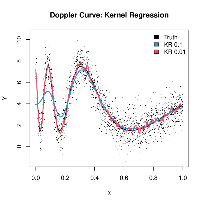
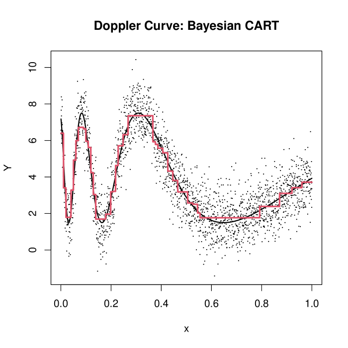
Figure 1: Doppler curve and (left) kernel regression estimates (ksmooth in R) with a bandwidth $0.1$ (capturing well the flat part) and $0.01$ (capturing well the wiggly part), (right) Bayesian CART posterior mean fit (wbart in the R package BART).

Brown and Low [11] showed asymptotic equivalence between (2.1) (with an equispaced fixed design) and (2.2) under a uniform smoothness assumption which is satisfied by, e.g., $\alpha$-Hölderian smooth functions with $\alpha>0.5$. From a sequence of optimal procedures in one problem, they also prescribed a construction of an asymptotically equivalent sequence in the other. This recipe is particularly convenient for linear estimators. For Bayesian methods, however, it is generally not known whether the knowledge of a (wavelet shrinkage/non-linear) minimax procedure in one problem automatically implies the optimality in the other. This is why we study Bayesian procedures in both models (see Section 3 for white noise and Section 4 for regression). We obtain local rate-optimality in regression under the assumption $\alpha>1/2$ in Section 4.2 and, finally, in Section 4.3 we show that a new class of adaptive-split priors (related to variable-knot spline techniques) yields exact-rate optimality without assuming $\alpha>1/2$.

In both models (2.1) and (2.2), the goal is to estimate a possibly spatially inhomogeneous function $f_{0}$ (see Section 2.1 below). We assess the quality of an estimator using both the global $L^{r}$ loss as well as the locally re-weighted supremum-norm loss (similarly as in [32]). In particular, for the (near) minimax rate $r_{n}(x)$ of adaptive estimation of $f_{0}$ at the point $x$, we will show that, with probability $P_{f_{0}}$ tending to one, the random variable

$$\sup_{x\in[0,1]}\frac{1}{r_{n}(x)}|f(x)-f_{0}(x)|,\quad\text{with}\quad f\sim\Pi(f\,|\>Y)$$ (2.6)

denoting the posterior distribution, is stochastically bounded, thereby implying a uniform local adaptation. Such spatial adaptation is not automatic for many standard estimators. We illustrate this phenomenon on two simulated examples below.

Example 1.

(Doppler Curve) Similarly as in [25] and [70], we generate $n=2048$ observations from a noisy Doppler curve (2.1) with $f_{0}(x)=3\sin[4/(x+0.2)]+1.5$ and $\sigma=1$ with $x_{i}=i/n$. This function has heterogeneous smoothness which cannot be captured with prototypical global smoothing methods such as global kernel regression (Figure 1 on the left) which leads to over/undersmoothing depending on the choice of a fixed kernel width. Tree-based methods, such as Bayesian CART, are better suited for this task by placing the splits more often in areas where the function is less smooth (Figure 1 on the right).

Example 2.

(Brownian Motion) The second example assumes $n=2^{11}$ where $f_{0}$ has been generated from a Brownian motion on $[0,1/2)$ (whose almost all trajectories are locally $\alpha$-Hölder continuous with $\alpha<1/2$) and a constant function on $[1/2,1]$. The plots of the kernel regression and Bayesian CART estimates are in Figure 2. Bayesian CART wastes no splits on the flat domain, showcasing its spatial adaptivity. We will investigate this example theoretically in Section 4.1 where we show that hierarchical Gaussian processes adapt to the worse regularity (determined by the Brownian motion). Beyond adaptability, Bayesian methods can also quantify uncertainty via the posterior (as seen from Figure 3 in Section 3.1.2). The width of the optimal band should be wider when the function is less smooth. In Section 3.1.2, we propose one such construction and show its frequentist validity.

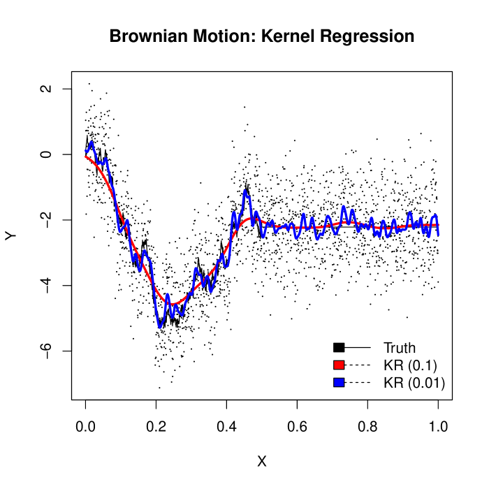
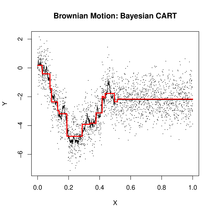
Figure 2: The Brownian motion example with (left) kernel regression estimates (ksmooth in R) with a bandwidth $0.1$ (capturing well the flat part of the curve) and $0.01$ (capturing well the wigglier part of the curve) and (right) Bayesian CART (posterior mean fit).

2.1 Spatially Inhomogeneous Functions

Below, we review several known facts about function classes with inhomogeneous smoothness. The Besov class $B_{p,q}^{\alpha}$ (which contains Hölder and Sobolev classes by setting $p=q=\infty$ and $p=q=2$, respectively) permits spatial inhomogeneity when $p<2$. For example, the Bump algebra (consisting of infinite mixtures of Gaussian bumps) coincides with $B_{1,1}^{1}$ [27] and constitutes an interesting caricature of smoothness inhomogeneity which would not be allowed within the Hölder class. Another example is the total variation (TV) class (contained inside $B_{1,\infty}^{1}$ and containing $B_{1,1}^{1}$) which includes functions that may have jumps localized in one part of the domain and be very flat elsewhere [27]. For a discussion on global minimax rates in Besov spaces we refer to [28, 21].

Function spaces where the smoothness can vary from point to point have quite a rich history. Besov spaces with variable smoothness were defined by [46] and later developed by many others (see [65] and references therein). We focus on Hölderian functions which are more intuitive for a supremum-norm analysis. Indeed, the perhaps more widely accepted notion of pointwise regularity has been formalized for Hölderian functions where the exponent itself is a function taking its values in $[0,\infty)$ [39, 1]. The question of which functions may be Hölder exponents was raised and partially answered in [19]. Andersson [1] later showed that a non-negative function is an exponent of a pointwise Hölder function if and only if it can be written as a limit inferior of a sequence of continuous functions. For example, ’typical’ functions in the Besov space exhibit a multifractal behavior where the Hölder exponent is a continuous function [39, 32].

Following [32], we define a set of bounded functions that are locally $t$-Hölder at $x\in\mathcal{[}0,1]$

$$\mathcal{C}(t,x,M,\eta)=\left\{f:[0,1]\rightarrow\mathbb{R};\max\left(\|f\|_{\infty},\sup_{0<|m|\leq\eta}\frac{|f(x+m)-f(x)|}{|m|^{t}}\right)\leq M\right\},$$ (2.7)

for $t\leq 1$. We denote with $\mathcal{C}(t,M,\eta)$ the set of functions that are locally Hölder for each $x\in[0,1]$, i.e. $\mathcal{C}(t,M,\eta)=\{f:f(x)\in\mathcal{C}(t,x,M,\eta)\,\,\forall x\in[0,1]\}$ . Throughout this work, we will make the following assumption on $f_{0}$.

Assumption 2.1.

Assume $f_{0}\in\mathcal{C}(t,M,\eta)$ where $M(\cdot)$ and $\eta(\cdot)$ are bounded and uniformly bounded away from zero and where the smoothness function $t(\cdot)$ satisfies $0<t_{1}\leq\inf_{x\in[0,1]}t(x)$.

It is well known that regularity, both local and global, of a function is reflected in the speed at which its wavelet coefficients decay. The following lemma formally characterizes the magnitude of multiscale coefficients in terms of the local Hölder smoothness.

Lemma 1.

Denote with $\beta_{lk}^{0}=\langle f_{0},\psi_{lk}\rangle$ the multiscale coefficient of a function $f_{0}$ that satisfies Assumption 2.1. Let $x\in[0,1]$ and for all $l>0$ define $k_{l}(x)\in\{0,1,\dots,2^{l}-1\}$ such that $x\in I_{l\,k_{l}(x)}$. For $l>0$ and $k\in\{0,1,\dots,2^{l}-1\}$ let

$$\eta_{lk}=\min_{x\in I_{lk}}\eta(x)\quad\text{ and}\quad M_{lk}=\max_{x\in I_{lk}}M(x).$$ (2.8)

When $l\geq\log_{2}[1/(2\eta_{l\,k_{l}(x)})]$, we have

$$|\beta_{l\,k_{l}(x)}^{0}|\leq 2\,M_{l\,k_{l}(x)}2^{-l[t(x)+1/2]}.$$ (2.9)

Proof.

For $k=k_{l}(x)$, we have $|\beta_{lk}^{0}|=2^{l/2}\left|\int_{k/2^{l}}^{(k+1/2)/2^{l}}[f_{0}(y)-f_{0}(y+2^{-l-1})]dy\right|$. Then

$$\begin{split}|\beta_{lk}^{0}|&\leq 2^{l/2}\int_{\frac{k}{2^{l}}}^{\frac{(k+1/2)}{2^{l}}}\left[|f_{0}(y)-f_{0}(x)|+|f_{0}(x)-f_{0}(y+2^{-l-1})|\right]dy\leq 2\,M_{lk}2^{-l[t(x)+1/2]}.\end{split}\qed$$

Remark 1.

One can obtain an alternative bound $|\beta_{lk}^{0}|\leq M_{lk}2^{-l(t_{lk}+1/2)}$ in terms of $t_{lk}=\min_{x\in I_{lk}}t(x)$ which follows directly from the definition of $\mathcal{C}(t,x,M,\eta)$.

Remark 2.

While in this paper we study the case $t(\cdot)\leq 1$, our results (Theorems 1, 2, 3 and 5) can be generalized to higher-order Hölder functions for which Lemma 1 applies with $S$-regular wavelet basis (see e.g. Extension 1 in [14] for more discussion and references).

3 Spatial Adaptation in White Noise

Donoho et al. [25] characterized pointwise (as well as global) properties of selective wavelet reconstructions showing their near-optimality for estimating Hölderian functions at a given point $x\in[0,1]$. Here, we establish uniform (supremum-norm) local adaptation for all $x\in[0,1]$ focusing on (2.6) under the white noise model (2.3) and various priors $\Pi(f)$. Adaptive supremum-norm concentration rate results (in white noise and regression) are still few and far between with pathbreaking progress made by multiple authors including [37, 75]. To date, results exist only for homogeneous Hölderian functions under the spike-and-slab prior [37, 75] and, more recently, the Bayesian CART prior [14]. Both of these priors leverage certain sparsity structure on the wavelet coefficients $\{\beta_{lk}\}$. We will show that both of these priors achieve uniform spatial adaptation.

3.1 Bayesian CART

CART methods [23, 15, 22] and other successful software developments including MARS [30] capture local aspects of the function being estimated by recursively subdividing the predictor space. Donoho et al. [25] pointed out that ‘the spatial adaptivity camp is, to date, a-theoretical and largely motivated by heuristic plausibility of the methods’. While it has been more than 20 years since this seminal paper, there is a shortage of theoretical justifications focusing on spatial adaptation with practically used machine learning methods. Here, we resurrect this question by focusing on Bayesian CART.

Bayesian CART corresponds to a wavelet prior that prescribes a particular sparsity structure in the wavelet reconstruction according to a binary tree $\mathcal{T}$ (see [14] for a more thorough exposition). A tree $\mathcal{T}$ is defined as a collection of hierarchically organized nodes $(l,k)$ where

$$(l,k)\in\mathcal{T}\Rightarrow(j,\lfloor k/2^{l-j})\in\mathcal{T}\quad\text{for}\quad j=0,\dots,l-1.$$ (3.1)

It will be useful to distinguish between two types of nodes: internal ones $\mathcal{T}_{int}=\{(l,k)\in\mathcal{T}:\{(l+1,2k),(l+1,2k+1)\}\in\mathcal{T}\}\cup(-1,0)$ and external ones $\mathcal{T}_{ext}=\mathcal{T}\backslash\mathcal{T}_{int}$ which are at the bottom of the tree. We then denote with $\boldsymbol{\beta}_{\mathcal{T}}=(\beta_{lk}:(l,k)\in\mathcal{T}_{int})$ the ‘active’ wavelet coefficients. Similarly as with the selective wavelet reconstruction (RiskShrink of [26]), Bayesian CART weeds out wavelet coefficients that are outside the tree, i.e. $\beta_{lk}=0$ when $(l,k)\notin\mathcal{T}_{int}$. Namely, for $L_{max}\equiv\lfloor\log_{2}n\rfloor$ we assume the tree-shaped wavelet shrinkage prior (Section 3 in [14])

$$\mathcal{T}\qquad \sim\qquad\Pi_{\mathcal{T}}$$ (3.2)

$$\{\beta_{lk}\}_{l\leq L_{max},k}\,|\>\mathcal{T}\ \sim\ \pi(\boldsymbol{\beta}_{\mathcal{T}})\,\otimes\bigotimes_{(l,k)\notin\mathcal{T}_{int}}\delta_{0}(\beta_{lk}),$$ (3.3)

where

$$\pi(\boldsymbol{\beta}_{\mathcal{T}})=\prod_{(l,k)\in\mathcal{T}_{int}}\phi(\beta_{lk};0,1)$$

is an independent product of standard Gaussians and where $\Pi_{\mathcal{T}}$ is the Bayesian CART prior [15]. This prior is essentially a heterogeneous Galton-Watson process with a node split probability

$$p_{lk}={P}[(l,k)\in\mathcal{T}_{int}]=p_{l}=(1/\Gamma)^{l}$$ (3.4)

for some $\Gamma>2$ (see Section 2.1 in [14] and [61]).

3.1.1 Uniformly Adaptive Rate

The following theorem establishes uniform spatial adaptation of Bayesian CART in the supremum-norm sense. In other words, the posterior is shown to contract at a locally minimax rate, up to a log factor, uniformly for all $x\in[0,1]$. While very intuitive, such a result has not yet been formalized in the Bayesian literature.

Theorem 1.

Assume the Bayesian CART prior (3.2) and (3.3) with a split probability (3.4) for some sufficiently large $\Gamma>0$. Under the model (2.3) and with $t,M$ and $\eta$ satisfying Assumption 2.1, we have

$$\sup\limits_{f_{0}\in\mathcal{C}(t,M,\eta)}E_{f_{0}}\Pi\left[f:\sup_{x\in[0,1]}\zeta_{n}(x)|f(x)-f_{0}(x)|>M_{n}\,\big{|}\,Y\right]\rightarrow 0$$ (3.5)

for $\zeta_{n}(x)=\left(\frac{n}{\log n}\right)^{\frac{t(x)}{2t(x)+1}}$ and for any $M_{n}\rightarrow\infty$ that is faster than $\sqrt{\log n}$.

The proof is provided in Section 7.1.

The first step in the proof of Theorem 1 is showing that trees, a-posteriori, grow deeper in domains where $f_{0}$ is less smooth. This property is summarized in Lemma 7 in the Supplemental Materials. Supremum-norm convergence rate results are valuable for constructing confidence bands. For example, Theorem 1 implies the non-parametric Bernstein-von Mises phenomenon in the multiscale space which can be used to construct credible bands with exact asymptotic coverage (see, e.g., Theorem 4.1 in [14]). This set, however, is not guaranteed to have the optimal size (i.e. its diameter shrinking at the minimax rate). Here, we will focus on constructing valid adaptive confidence bands. With spatially varying functions (such as the local Hölder functions from Section 2.1), one would expect the width of the confidence band to vary with the smoothness $t(\cdot)$ and be wider where $t$ is smaller. Keeping the diameter constant throughout may yield bands that are more conservative in certain areas of the sample space.

3.1.2 Locally Adaptive Bands

A reasonable requirement for band construction is that their diameter shrinks at the minimax rate of estimation, up to possibly a slow multiplication factor. When the degree of smoothness is known, multiscale credible balls can be constructed (see (5) in [13]) and intersected with qualitative restrictions on $f_{0}$ to obtain ‘optimal’ frequentist confidence sets (which shrink at the optimal rate).

We construct optimal confidence sets when the smoothness $t(\cdot)$ is unknown and varying over $[0,1]$. Confidence bands that are simultaneously adaptive and honest, of course, do not exist in full generality [48]. Gine and Nickl [35] point out, however, that such confidence sets exist for certain generic subsets of Hölderian functions, the so-called self-similar functions [55, 12, 33, 53, 58], whose complement was shown to be negligible [12]. Under self-similarity, [58, 14] constructed adaptive credible bands for homogeneous Hölderian functions under the spike-and-slab prior and the Bayesian CART, respectively.

Here, we extend the notion of self-similarity to inhomogeneous Hölder classes for which it is possible to construct a locally adaptive confidence set $\mathcal{C}_{n}$ in the sense that

$$\sup_{f,g\in\mathcal{C}_{n}}\left[\sup_{x\in[0,1]}\frac{\zeta_{n}(x)}{v_{n}}|f(x)-g(x)|\right]=\mathcal{O}_{P_{f_{0}}}(1)$$ (3.6)

for some suitable sequence $v_{n}\rightarrow\infty$ and where $\zeta_{n}(x)=(n/\log n)^{t(x)/(2t(x)+1)}$. Note that the diameter of $\mathcal{C}_{n}$ depends on $x$ and equals the minimax rate of estimation (inflated by $v_{n}$) at every point $x\in[0,1]$. Below, we formally introduce the notion of locally self-similar functions.

Definition 1.

(Local Self-Similarity) We say that $f\in\mathcal{C}(t,M,\eta)$ is locally self-similar at $x\in[0,1]$ if, for some $c_{1}>0$ and an integer $j_{0}$,

$$|K_{j}(f)(x)-f(x)|\geq 2^{-j\,t(x)}c_{1}\quad\text{for all }j\geq j_{0},$$ (3.7)

where $K_{j}(f)=\sum_{l\leq j-1}\sum_{k}\,\langle\psi_{lk},f\rangle\,\psi_{lk}$ is the wavelet projection at level $j$. The class of all self-similar functions at $x$ will be denoted by $\mathcal{C}_{SS}(t(x),x,M(x),\eta(x))$. Moreover, we denote with $\mathcal{C}_{SS}(t,M,\eta)$ a set of functions that are self-similar for all $x\in[0,1]$.

For spatially heterogeneous Hölderian functions, we construct locally adaptive confidence bands whose width is varying and reflects smoothness at each given $x$ While related to previous constructions (see e.g. [14] for the homogeneous case), its simplicity and ease of computability make our band particularly appealing in practice (see Figure 3). In addition, we are not aware of any other related frequentist band for the case of heterogeneous smoothness. We center our confidence bands around a pivot estimator, the median tree estimator [14].

Definition 2.

(The Median Tree) Given a posterior distribution $\Pi_{\mathcal{T}}[\cdot\,|\,Y]$ over tree-shaped coefficient subsets, we define the median tree $\mathcal{T}^{*}_{Y}$ as the following set of nodes

$$\mathcal{T}^{*}_{Y}=\left\{(l,k),\ l\leq L_{max},\ \ \Pi[(l,k)\in\mathcal{T}_{int}\,|\,Y]\geq 1/2\right\}.$$ (3.8)

We define the resulting median tree estimator as

$$\widehat{f}_{T}(x)=\sum_{(l,k)\in\mathcal{T}^{*}_{Y}}Y_{lk}\psi_{lk}(x)$$ (3.9)

which is shown to attain the near-minimax rate of estimation at each point (see the proof of Theorem 2). Next, we define the local radius (which varies with $x$) as

$$\sigma_{n}(x)=v_{n}\sqrt{\frac{\log{n}}{n}}\sum_{l=0}^{L_{max}}\mathbb{I}\{(l,k_{l}(x))\in\mathcal{T}_{Y}^{*}\}|\psi_{lk_{l}(x)}(x)|$$ (3.10)

for some $v_{n}\rightarrow\infty$ to be chosen. Finally, we construct the confidence band according to the following prescription

$$\mathcal{C}_{n}=\left\{f:\sup_{x\in[0,1]}\left[\frac{1}{\sigma_{n}(x)}|f(x)-\widehat{f}_{T}(x)|\right]\leq 1\right\},$$ (3.11)

where $\widehat{f}_{T}$ is as in (3.9) and $\sigma_{n}(x)$ is as in (3.10).

Theorem 2.

Let $\Pi$ be the prior as in the statement of Theorem 1. Then for $\mathcal{C}_{n}$ defined in (3.11), uniformly over $t,M$ and $\eta$ that satisfy the Assumption 2.1, as $n\to\infty$,

$$\inf_{f_{0}\in\mathcal{C}_{SS}(t,M,\eta)}P_{f_{0}}(f_{0}\in\mathcal{C}_{n})\to 1.$$

Uniformly over $f_{0}\in\mathcal{C}_{SS}(t,M,\eta)$, the diameter verifies (7.21), as $n\to\infty$, and the credibility of the band satisfies

$$\Pi[\mathcal{C}_{n}\,|\,X] =1+o_{P_{f_{0}}}(1).$$ (3.12)

The proof is provided in Section 7.2.

According to Theorem 2, the band (3.11) has asymptotic coverage $1$. It is possible to intersect (3.11) with a multi-scale ball (similarly to [58, 14]) to obtain asymptotic coverage $1-\gamma$ for some small $\gamma>0$ as a consequence of the non-parametric Bernstein-von Mises (BvM) theorem. In order to illustrate the practical usefulness of Theorem 2, we revisit the Brownian motion example (Example 2) from Figure 3. We implement a dyadic version of the Bayesian CART algorithm [15] which splits only at dyadic rationals (as opposed to Figure 2 (on the right) where Bayesian CART splits at observed values). We plot the adaptive band (3.11) choosing $v_{n}=2$ together with a non-adaptive band obtained by taking the maximal diameter $\sigma(x)$ over the domain $[0,1]$ (as in Theorem 4 of [14]). We can see the benefits of our adaptive construction, where the width is larger in the first half of the domain where the function meanders according to the Brownian motion (expected since the smoothness is smaller than $1/2$). Compared with Figure 3 on the right, the point-wise $95\%$ credible band does not yield satisfactory coverage on this example.

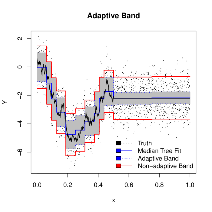
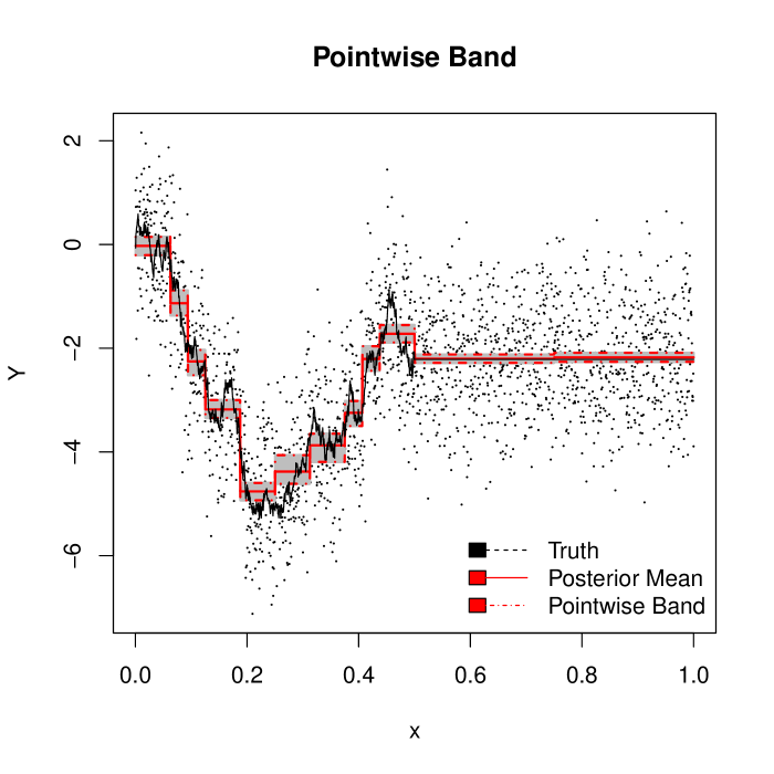
Figure 3: The Brownian motion example (Example 2) with dyadic Bayesian CART. (left) Adaptive confidence band (3.11) (blue) and non-adaptive band (red). (right) Point-wise $95\%$ credible intervals.

3.2 Spike-and-Slab Priors

Spike-and-slab priors are arguably one of the most ubiquitous priors in statistics (see references [17, 37, 58] for wavelet shrinkage contexts). Compared with the Bayesian CART prior from Section 3.1, spike-and-slab priors allocate positive prior mass to any subset $\mathcal{T}$ of $\{(l,k):l\leq L_{max}\}$, not just tree-shaped subsets. We define the spike-and-slab prior through the following hierarchical model.

Assumption 3.1.

(Spike-and-Slab Prior)

• Prior on $\mathcal{T}\subseteq\{(l,k):0\leq k<2^{l},l\leq L_{max}\}$: There exist constants $c_{T},C_{T}>0$ such that

  $$c_{T}\,\omega_{l}\leq\frac{\Pi(\mathcal{T}\cup\{(l,k)\})}{\Pi(\mathcal{T})}\leq C_{T}\,\omega_{l}\quad\forall\mathcal{T}\,\,\text{such that}\,\,(l,k)\notin\mathcal{T}$$ (3.13)

  for some positive sequence $\omega_{l}$ such that, for some $B_{\omega}>0$ and $\delta>0$,

  $$n^{-B_{\omega}}\leq\omega_{l}\leq n^{(1-\delta)/2}2^{-l}\quad\text{for}\quad l\leq L_{max}.$$ (3.14)

• There exist probability densities $\pi_{lk}(\cdot)$ on $\mathbb{R}$ such that, conditionally on $\mathcal{T}$,

  $$\beta_{lk}\stackrel{{\scriptstyle ind}}{{\sim}}\pi_{lk}\quad\forall(l,k)\in\mathcal{T}\quad\text{and}\quad\beta_{lk}=0,\quad\forall(l,k)\notin\mathcal{T}$$

  and there exist $R,c_{R},C_{R}>0$ such that

  $$c_{R}\leq\inf_{|\beta|\leq R}\pi_{lk}(\beta)\leq\sup_{\beta\in\mathbb{R}}\pi_{lk}(\beta)\leq C_{R}.$$ (3.15)

While seemingly similar to the prior considered in [37], our Assumption 3.1 is much weaker. Indeed, our prior construction subsumes the spike-and-slab prior of [37] by imposing weaker constraints on the decay of inclusion probabilities. Note that $\omega_{l}$’s in (3.14) are allowed to be much larger than in [37] which assume $n^{-B}\leq\omega_{l}\leq 2^{-j(1+\tau)}$ for some $\tau>1/2$. This perhaps subtle difference is of great practical importance and indicates that optimal sup-norm adaptation occurs in far less sparse situations than originally perceived. Another important difference is that we do not require the binary indicators $\mathbb{I}(\beta_{lk}\neq 0)$ for $0\leq k<2^{l}$ and $l\leq L_{max}$ to be iid Bernoulli random variables. This extension allows us to consider, for example, Ising prior constructions [7] which allow the inclusion indicators to be related through a Markovian model.

Theorem 3.

Consider the model (2.3) with a prior $\Pi$ on $\{\beta_{lk}\}_{lk}$ following the Assumption 3.1. Let $t,M$ and $\eta$ satisfy the Assumption 2.1. Then

$$\sup_{f_{0}\in\mathcal{C}(t,M,\eta)}E_{f_{0}}\Pi\left[f:\sup_{x\in[0,1]}\zeta_{n}(x)|f(x)-f_{0}(x)|>\widetilde{M}\,\big{|}\,Y\right]\rightarrow 0,$$

for all sufficiently large $\widetilde{M}>0$ where $\zeta_{n}(x)=(n/\log n)^{t(x)/(2t(x)+1)}$.

The proof is provided in Section 7.3.

Theorem 3 shows that, unlike Bayesian CART, the spike-and-slab priors achieve the exact rate uniformly over the entire domain $[0,1]$ without any additional logarithmic penalty ([14] showed that the log-factor in Bayesian CART is non-negotiable). In Lemma 11 (an analog of Lemma 1 in [37]) we show that the posterior concentrates on a subset of large enough coefficients. This fact can be used to show that the median probability model (MPM) [4, 5, 58] consisting of all coefficients with at least $50\%$-posterior probability of being active is an (exact) rate-optimal estimator. Following the strategy of Proposition 4.5 in [58] one can then show that Theorem 2 remains true for the spike-and-slab prior when replacing the median tree estimator with MPM and with $v_{n}$ that can grow slower at a rate at least $\sqrt{\log n}$ [58].

4 Spatial Adaptation in Non-parametric Regression

Throughout this section, we assume the canonical non-parametric regression setup (2.1) with $\sigma^{2}=1$. While nonparametric regression with a regular design and the white noise model are asymptotically equivalent (e.g. under the usual smoothness assumption $t(x)>1/2$ [11]), optimality of a procedure in one setup does not automatically imply optimality in the other. In Section 4.2, we show rate-optimality of Bayesian CART in non-parametric regression when $t(x)>1/2$ without assuming regular designs. Later in Section 4.3, we relax the restriction $t(x)>1/2$ and propose new ‘repulsive’ partitioning priors (related to adaptive-knot splines) and show that they are exact-rate adaptive. First, we describe some not so optimistic findings for hierarchical Gaussian priors.

4.1 Gaussian Processes

In Figure 1 and 2 we have seen that spatial adaptation is not attainable by methods which are not sufficiently localized. In this section, we formally show that several practically used Gaussian process priors do not lead to spatially adaptive concentration rates. While this phenomenon is not entirely surprising, it is nevertheless worthwhile to document it formally. In particular, we provide lower bound results showing sub-optimality of Gaussian processes in terms of a global estimation loss. To this end, we consider the following heterogeneous-smoothness assumption which aligns with Figure 2 where the function $f_{0}$ has smoothness $\alpha_{1}<1/2$ on $[0,1/2]$ and $\alpha_{2}=1$ on $(1/2,1]$.

Assumption 4.1.

Assume that the Haar wavelet decomposition of a function $f_{0}$ satisfies (with $I_{l}=\{0,1,\dots,2^{l}-1\}$)

$$f_{0}(x)=\psi_{-10}(x)\beta_{-10}^{0}+\sum_{l=0}^{\infty}\sum_{k\in I_{l}}\beta^{0}_{lk}\psi_{lk}(x)$$ (4.1)

where (for $I_{l1}\cup I_{l2}=I_{l}$ with $|I_{l1}|\asymp|I_{l2}|$ and some $M_{1}>0$)

$$\max_{k\in I_{l1}}|\beta^{0}_{lk}|\leq M_{1}2^{-l(\alpha_{1}+1/2)}\quad\text{and}\quad\max_{k\in I_{l2}}|\beta^{0}_{lk}|\leq M_{1}2^{-l(\alpha_{2}+1/2)}\quad\text{with}\quad\alpha_{1}<\alpha_{2}.$$ (4.2)

Methods that are globally, but not locally, adaptive are expected to adapt to the worse-case scenario and attain the slower rate determined by the smaller smoothness $\alpha_{1}$. We will formalize this intuition by assessing the quality of the reconstruction with an $L^{2}$ loss over the entire domain as well as the smoother domain determined by $\alpha_{2}$, i.e. we define

$$\|f-f_{0}\|_{2}^{2}\equiv\int_{0}^{1}|f(x)-f_{0}(x)|^{2}dx\quad\text{and}\quad\|f-f_{0}\|_{1/2,1}^{2}\equiv\int_{1/2}^{1}|f(x)-f_{0}(x)|^{2}dx.$$

We now consider three hierarchical Gaussian processes on

$$f(x)=\psi_{-10}(x)\beta_{-10}+\sum_{l=0}^{\infty}\sum_{k\in I_{l}}\beta_{lk}\psi_{lk}(x)$$ (4.3)

induced through a prior on the sequence $\{\beta_{lk}\}_{lk}$. These priors were studied in [59]. This section assumes a regular design $x_{i}=i/n$ for $n=2^{L_{max}+1}$ with some $L_{max}>0$.

• (T1) (Sieve Prior) Given a truncation level $1\leq L\leq L_{max}$ and some fixed $\tau>0$ we have

  $$\beta_{lk}\stackrel{{\scriptstyle iid}}{{\sim}}\mathcal{N}(0,\tau^{2})\quad\text{for}\quad l\leq L\quad\text{and}\quad\beta_{lk}=0\quad\text{for}\quad l>L.$$

  The truncation level $L$ is assigned a prior $\pi(L)$ which satisfies Lemma 3.4 in [59] (e.g. a hypergeometric or a Poisson prior distribution).

• (T2) (Scale Parameter) Given $\alpha>0$ assume

  $$\beta_{lk}=\begin{cases}2^{-l(\alpha+1/2)}Z_{lk}\quad\text{where}\quad Z_{lk}\stackrel{{\scriptstyle iid}}{{\sim}}\mathcal{N}(0,\tau^{2})\quad&\text{for}\quad l\leq L_{max}\\ 0\quad&\text{for}\quad l>L_{max}\end{cases}$$

  where the scale parameter arrives from $\tau\sim\pi_{\tau}$, with $\pi_{\tau}$ satisfying the assumptions of Lemma 3.5 of [59] (e.g. an inverse gamma or a Weibull distribution).

• (T3) (Rate Parameter) Given $\tau>0$ assume

  $$\beta_{lk}=\begin{cases}2^{-l(\alpha+1/2)}Z_{lk}\quad\text{where}\quad Z_{lk}\stackrel{{\scriptstyle iid}}{{\sim}}\mathcal{N}(0,\tau^{2})\quad&\text{for}\quad l\leq L_{max}\\ 0\quad&\text{for}\quad l>L_{max}\end{cases}$$

  where the ‘smoothness’ parameter $\alpha$ arrives from $\alpha\sim\pi_{\alpha}$ satisfying the assumptions of Lemma 3.6 of [59] (e.g. a gamma distribution).

These priors have been studied in a multitude of works, see e.g. [2, 66] for the setup (T1) [6, 42, 69] for the Gaussian process priors (T2) and (T3). More recently, this framework has been studied in [59] in the case of Fourier-series priors where both lower bounds and an upper bound have been obtained in the case of non-linear regression. We adapt their proof to the wavelet basis case with functions satisfying (4.2). In this case, we note that for any $L$ such that $2^{L}\leq n$ and for $f_{\beta,L}$ denoting the Haar wavelet expansions (4.3) truncated at $L\geq 1$ we have for $x_{i}=i/n$

$$\|f_{\beta,L}-f_{\beta_{0},L}\|_{n}^{2}=\frac{1}{n}\sum_{i}[f_{\beta,L}(x_{i})-f_{\beta_{0},L}(x_{i})]^{2}=\|\boldsymbol{\beta}_{L}-\boldsymbol{\beta}_{0,L}\|_{2}^{2}=\|f_{\beta,L}-f_{\beta_{0},L}\|_{2}^{2}.$$

where $\boldsymbol{\beta}_{L}=(\beta_{lk}:l\leq L)^{\prime}$ (resp. $\boldsymbol{\beta}_{0,L}$ ) is the truncated version of $\boldsymbol{\beta}$ (resp $\boldsymbol{\beta}_{0}$).

Theorem 4.

Let $f_{0}$ satisfy (4.2) and consider either of the priors (T1)-(T3). Then for $Y=(Y_{1},\dots,Y_{n})^{\prime}$ arising from (2.1) with $x_{i}=i/n$ we have

$$\Pi\left[\|f-f_{0}\|_{2}\leq M_{n}\epsilon_{n}(\alpha_{1})\,|\>Y\right]=1+o_{P_{f_{0}}}(1)\quad\text{as $n\rightarrow\infty$}$$ (4.4)

with

$$\epsilon_{n}(\alpha_{1})=\begin{cases}&(n/\log n)^{-\alpha_{1}/(2\alpha_{1}+1)}\quad\text{under (T1), (T2) if $\alpha_{1}<2\alpha+1$, and (T3)}\\ &(n/\log n)^{-(2\alpha+1)/(4\alpha+4)}\quad\text{under (T2) if $\alpha_{1}\geq 2\alpha+1$}.\end{cases}$$

Moreover, for all functions satisfying (4.2) and, for some $c>0$,

$$\min_{k\in I_{l1}}|\beta^{0}_{lk}|\geq c\,2^{-l(\alpha_{1}+1/2)}$$ (4.5)

we have for all $\delta>0$

$$\Pi\left[\|f-f_{0}\|_{1/2,1}\leq n^{-\delta}\epsilon_{n}(\alpha_{1})\,|\>Y\right]=o_{P_{f_{0}}}(1)\quad\text{as $n\rightarrow\infty$}.$$ (4.6)

The proof is provided in Section 8.

The first statement (4.4) shows that the posterior under the Gaussian sequence priors adapts to the worse smoothness $\alpha_{1}$. Moreover, the second statement (4.6) implies that, under a suitable identifiability condition, the posterior is incapable of achieving a faster rate on the smoother domain (determined by $\alpha_{2}>\alpha_{1}$), rendering adaptation to $\alpha_{2}$ impossible. Note that similarly to [59], the same conclusions holds if one deploys an empirical Bayesian procedure based on the marginal maximum likelihood estimator on $L$ for T1 (resp. $\tau$ for T2 and $\alpha$ for T3).

4.2 Bayesian CART

This section reports positive findings in the context Bayesian CART. In particular, we show a regression analogue of Theorem 1 assuming $t(x)>1/2$. [14] also study Bayesian CART in regression but with a regular design where the prior is assigned to empirical wavelet coefficients. This re-parametrization closely resembles the white noise model, enabling a more direct transfer of the results. Here, we follow an alternative route. A perhaps more transparent approach is to assign a prior directly to the actual (not empirical) wavelet coefficients (similarly as in [75]). This strategy aligns more closely with what is done in practice. We pursue this direction here and, in addition, consider designs that are not necessarily regular.

With a vector of observations $Y=(Y_{1},\dots,Y_{n})^{\prime}$ and $F_{0}=(f_{0}(x_{1}),\dots,f_{0}(x_{n}))^{\prime}$, we can re-write (2.1) in a matrix notation as

$$Y=X\boldsymbol{\beta}_{0}+\boldsymbol{\nu},\quad\text{where}\quad\boldsymbol{\nu}=F_{0}-X\boldsymbol{\beta}_{0}+\boldsymbol{\epsilon}\quad\text{with}\quad\boldsymbol{\epsilon}\sim\mathcal{N}(0,I_{n}),$$ (4.7)

where $\boldsymbol{\beta}_{0}=(\beta^{0}_{1},\dots,\beta^{0}_{p})^{\prime}\in\mathbb{R}^{p}$ is a sparse vector of multiscale coefficients $\langle f_{0},\psi_{lk}\rangle$ ordered according to $2^{l}+k$ and where $X=[X_{1},\dots,X_{p}]$ is an $(n\times p)$ Haar wavelet design matrix constructed as follows. The matrix $X=(x_{ij})$ consists of $p$ wavelet bases $\psi_{lk}$ up to a resolution $L_{max}$ which satisfies $p=2^{L_{max}}=\lfloor C^{*}\sqrt{n/\log n}\rfloor$ for some suitable $C^{*}>0$. The columns in $X$ are implicitly ordered according to the index $2^{l}+k$ (from the smallest to the largest), where

$$x_{ij}=\psi_{lk}(x_{i})\quad\text{with}\quad j=2^{l}+k.$$

Because we assume $t(x)>1/2$, we do not need resolutions larger than $L_{max}$ to be able to approximate $f_{0}$ well. We will be denoting with $\mathbb{T}$ all tree-shaped subsets of nodes $(l,k)$ such that $l\leq L_{max}$. For a tree $\mathcal{T}\in\mathbb{T}$ and a vector $\boldsymbol{\beta}\in\mathbb{R}^{p}$, we denote with $\boldsymbol{\beta}_{\mathcal{T}}$ the subset of coefficients inside the tree and with $\boldsymbol{\beta}_{\backslash\mathcal{T}}$ the complement. Similarly, we split the design matrix $X$ into active covariates $X_{\mathcal{T}}$ (that correspond to $(l,k)\in\mathcal{T}_{int}$) and the complementary inactive ones $X_{\backslash\mathcal{T}}$. It will be advantageous to use the unit-information $g$-prior for $\boldsymbol{\beta}_{\mathcal{T}}$

$$\boldsymbol{\beta}_{\mathcal{T}}\sim\mathcal{N}(0,g_{n}(X_{\mathcal{T}}^{\prime}X_{\mathcal{T}})^{-1})\quad\text{with $g_{n}=n$}$$ (4.8)

which yields the following marginal likelihood under each tree $\mathcal{T}$

$$N_{\mathcal{T}}(Y)=\frac{1}{(2\pi)^{n/2}(1+g_{n})^{|\mathcal{T}|/2}}\exp\left\{-\frac{1}{2}Y^{\prime}[I-X_{\mathcal{T}}\Sigma_{\mathcal{T}}X_{\mathcal{T}}^{\prime}]Y\right\},$$

where

$$\Sigma_{\mathcal{T}}=c_{n}(X_{\mathcal{T}}^{\prime}X_{\mathcal{T}})^{-1}\quad\text{with $c_{n}=g_{n}/(g_{n}+1)$}.$$

Throughout this section, we will denote with $n_{lk}^{L}$ (resp. $n_{lk}^{R}$) the number of observations that fall inside the domain of the left (resp. right) wavelet piece $\psi_{lk}$, i.e. $n_{lk}=\sum_{i=1}^{n}\mathbb{I}(x_{i}\in I_{lk})=n_{lk}^{R}+n_{lk}^{L}$ and we define

$$\bar{n}_{lk}=\max\{n_{lk}^{R},n_{lk}^{L}\}\quad\text{and}\quad\underaccent{\bar}{n}_{lk}=\min\{n_{lk}^{R},n_{lk}^{L}\}.$$

The regular design $x_{i}=i/n$ satisfies $\bar{n}_{lk}=\underaccent{\bar}{n}_{lk}=n/2^{l+1}$. Here, we assume a fixed design $\mathcal{X}=\{x_{i}\in[0,1]:1\leq i\leq n\}$ that is not necessarily regular. Instead, we make the following design balance assumption.

Assumption 4.2.

(Balanced Design)  Let $\widetilde{L}_{max}$ be such that $2^{\widetilde{L}_{max}}=\mathcal{O}(n/\log n)$. We say that the design $\mathcal{X}$ is $\upsilon$-regular for some $\upsilon>0$ if for any $(l,k)$ s.t. $0\leq l\leq\widetilde{L}_{max}$

$$\frac{c\,n}{2^{l}}\leq\underaccent{\bar}{n}_{lk}\leq\bar{n}_{lk}\leq\frac{(C+l)n}{2^{l}}\quad\text{for some $c,C>0$}$$ (4.9)

and, for some $C_{d}>0$,

$$0\leq\bar{n}_{lk}-\underaccent{\bar}{n}_{lk}\leq C_{d}\frac{\sqrt{n}\log^{\upsilon}n}{2^{l/2}}.$$ (4.10)

Note that the threshold $L_{max}$ used to construct the design matrix $X$ is smaller than the threshold $\widetilde{L}_{max}$ in Assumption 4.2 and all partitioning cells induced by $\mathcal{T}\in\mathbb{T}$ are guaranteed to have at least one observation. The Assumption 4.2 is not overly restrictive. Indeed, we show in Lemma 14 (Supplemental Materials) that (4.10) is satisfied with probability approaching one when $\mathcal{X}$ arises from a uniform distribution on $[0,1]$ for $\upsilon\geq 1/2$. Irregular observations ultimately induce correlated Haar wavelet designs $X$ where the correlation pattern has a particular hierarchical structure described in the following lemma.

Lemma 2.

Let $X_{i}$ and $X_{j}$ be columns of $X$ that correspond to nodes $(l_{2},k_{2})$ and $(l_{1},k_{1})$, respectively. Then we have

$$|X_{j}^{\prime}X_{i}|=0 \,\,\text{when}\,\,(l_{2},k_{2})\,\,\text{is {\em not} a descendant of $(l_{1},k_{1})$},$$

$$|X_{j}^{\prime}X_{i}|\leq 2^{\frac{l_{1}+l_{2}}{2}}|n_{l_{2}k_{2}}^{L}-n_{l_{2}k_{2}}^{R}| \,\,\text{when}\,\,(l_{2},k_{2})\,\,\text{is a descendant of $(l_{1},k_{1})$}.$$

Proof.

When $(l_{2},k_{2})$ is not a descendant of $(l_{1},k_{1})$, the domains of $\psi_{l_{1}k_{1}}$ and $\psi_{l_{2}k_{2}}$ do not overlap, yielding orthogonality. When $(l_{2},k_{2})$ is a descendant of $(l_{1},k_{1})$, the wavelet domains satisfy $I_{l_{2}k_{2}}\subset I_{l_{1}k_{1}}$ and $X_{j}^{\prime}X_{i}$ will be (up to a sign) equal to the size of the amplitude product $2^{(l_{1}+l_{2})/2}$ multiplied by the excess number of observations falling inside the longer wavelet piece $\psi_{l_{2},k_{2}}$.∎

As with other related consistency results in regression (see e.g. [52]), we cannot allow for too much correlation in the design $X$. Fortunately, balanced designs that satisfy Assumption 4.2 are not too collinear and yield diagonally dominant covariance matrices with well-behaved eigenvalues (see Lemma 3 below).

Lemma 3.

(Eigenvalue Bounds) Under the Assumption 4.2 with $0\leq\upsilon\leq 1/2$ and some suitable $c>0$, the eigen-spectrum of $X_{\mathcal{T}}^{\prime}X_{\mathcal{T}}$ for each $\mathcal{T}\in\mathbb{T}$ satisfies

$$\underaccent{\bar}{\lambda}\,n\leq\lambda_{min}(X_{\mathcal{T}}^{\prime}X_{\mathcal{T}})\leq\lambda_{max}(X_{\mathcal{T}}^{\prime}X_{\mathcal{T}})\leq\bar{\lambda}\,n\,\log n\quad\text{for some $0<\underaccent{\bar}{\lambda}\leq\bar{\lambda}$}.$$ (4.11)

The proof is provided in Section 11.0.2.

We are now ready to state a non-parametric regression version of Theorem 1.

Theorem 5.

Assume the regression model (4.7) under Assumption 4.2 for some $0\leq\upsilon\leq 1/2$ and $c,C,C_{d}>0$. Assume the Bayesian CART tree prior $\Pi_{\mathcal{T}}$ with a split probability $p_{l}=(\Gamma)^{-l^{2}}$ for some sufficiently large $\Gamma>0$ and the $g$-prior (4.8). Assume that $t,M$ and $\eta$ satisfy Assumption 2.1 with $t_{1}>1/2$, then

$$\sup_{f_{0}\in\mathcal{C}(t,M,\eta)}E_{f_{0}}\Pi\left[f:\sup_{x\in[0,1]}\zeta_{n}(x)|f(x)-f_{0}(x)|>M_{n}\,\big{|}\,Y\right]\rightarrow 0$$

for $\zeta_{n}(x)=\left(\frac{n}{\log n}\right)^{\frac{t(x)}{2t(x)+1}}$ and for any $M_{n}\rightarrow\infty$ that is faster than ${\log^{1/2}n}$.

The proof is provided in Section 6.1.

Note that the prior split probability decays more rapidly, i.e. $p_{l}=(\Gamma)^{-l^{2}}$, to accommodate the irregular design assumption. An analogous statement can be obtained for the spike-and-slab prior using a similar approach as in the proof of Theorem 3. In addition, the confidence set construction in (3.11) remains valid also under the non-parametric regression setting. Indeed, rate-optimality of the posterior implies rate-optimality of the median-tree estimator and the regression variant of Theorem 2 thus holds under the assumption $t_{1}>1/2$.

4.3 Repulsive Partition Prior

In the previous section, we studied a prior on wavelet coefficients that corresponds to recursive partitioning. In this section, we propose a different partitioning prior on piecewise constant functions which relates to variable knot spline techniques [50, 70]. We assume that a partition $S=(I_{1}^{S},\cdots,I_{J}^{S})$ of $[0,1]$ is not necessarily induced by a tree but arrives from a ‘determinantal-type’ prior

$$S\sim\pi_{S}\propto\prod_{j=1}^{J}|I_{j}^{S}|^{B}\mathbb{I}(S\in\mathbb{S})\quad\text{for some $B>0$},$$ (4.12)

where $\mathbb{S}$ contains all partitions made out of blocks with endpoints belonging to a fixed grid $\mathcal{I}_{n}=(z_{\ell}:\ell\leq N_{n})$ such that $z_{0}=0$ and $z_{N_{n}}=1$ and

$$0\leq z_{\ell}<z_{\ell+1},\,\,\frac{C_{1}\log n}{n}\leq z_{\ell+1}-z_{\ell}\leq\frac{C_{2}\log n}{n},\,\,\ell\leq N_{n}\quad\text{for some}\quad C_{1},C_{2}>0.$$ (4.13)

Note that the size of an interval in $S$ can be measured either in terms of its length or in terms of its number of units, i.e. number of elements in the grid $\mathcal{I}_{n}$ belonging to it.

We refer to (4.12) as a repulsive partitioning prior because it prevents the splits from occurring too close to one another. The prior (4.12) thus rewards partitions that are more regular. The set $\mathcal{I}_{n}$ contains candidate knots for possible split, e.g. a subset of observed design points. While in variable knot spline techniques (such as MARS [30]) knot points are added, removed and allocated recursively using cross-vaildiation, here we let the posterior distribution choose the knots in a data-adaptive way.

Given the partition $S\in\mathbb{S}$ we reconstruct the regression surface with

$$\begin{split}f_{\beta}^{S}(x)&=\sum_{j=1}^{J}\beta_{j}\mathbb{I}_{I_{j}^{S}}(x),\quad\text{where}\quad(\beta_{j}:j\leq J)\stackrel{{\scriptstyle ind}}{{\sim}}g_{j}.\\ \end{split}$$ (4.14)

Regarding the prior density $g_{j}$, we will assume that there exist $0<c_{0}\leq c_{1}$ and $B_{0}>0$ such that

$$c_{0}\leq g_{j}(\beta)\quad\forall|\beta|\leq B_{0},\quad\text{and}\quad\|g_{j}\|_{\infty}\leq c_{1}\quad\forall j\leq J.$$ (4.15)

While in Section 4.2 we obtained the near-minimax rate under the assumption $t_{1}>1/2$, here we show rate-exactness without necessarily assuming $t_{1}>1/2$. We are interested in bounding $\Pi(A_{\varepsilon_{n}}^{c}(\widetilde{M})\,|\>D_{n})$ where $D_{n}=\{(Y_{i},x_{i})\}_{i=1}^{n}$ and

$$A_{\varepsilon_{n}}(\widetilde{M})=\left\{\sup_{x\in(0,1)}\frac{|f_{\beta}^{S}(x)-f_{0}(x)|}{\varepsilon_{n}(x)}\leq\widetilde{M}\right\}\quad\text{and}\quad\varepsilon_{n}(x)=\left(\frac{n}{\log n}\right)^{-\frac{t(x)}{2t(x)+1}}.$$ (4.16)

For a given point $x\in[0,1]$ and a partition $S=\{I_{j}^{S}\}_{j=1}^{J}$ we denote with $I_{x}^{S}\in S$ the interval containing $x$ and with $R(I_{x}^{S})$ (resp. $L(I_{x}^{S})$) its right (resp. left) neighbor. We then define $\mathcal{I}(x)$ as the set of intervals which contain $x$ and the two neighboring intervals, i.e.

$$\mathcal{I}(x)=\bigcup_{S\in\mathbb{S}}\{I_{x}^{S},R(I_{x}^{S}),L(I_{x}^{S})\},$$ (4.17)

and we define, for a given $x\in[0,1]$ and some $u_{1}>0$,

$$\Omega_{n,x}(u_{1})=\left\{|n_{I}-n\times p_{I}|\leq u_{1}\sqrt{\log n\times n\times p_{I}}\quad\forall I\in\mathcal{I}(x)\right\}$$ (4.18)

where $n_{I}=\sum_{i=1}^{n}\mathbb{I}(x_{i}\in I)$ and $p_{I}$ is a function of $I$ which satisfies $p_{0}|I|\leq p_{I}\leq p_{1}|I|$ for some $0<p_{0}\leq p_{1}$. Our results will be conditional on a large probability event which can be loosely regarded as a design assumption. Namely, we require that the cells containing the knot points $z_{l}$ (and the neighboring cells) are large enough in terms of the number of observations falling inside, i.e. we consider an intersection of events in (4.18)

$$\Omega_{n}(u_{1})=\bigcap_{l=1}^{N_{n}}\Omega_{n,z_{l}}(u_{1}).$$

Our result below will hold on this event. If the design is regular, then $\Omega_{n}(u_{1})$ holds for any $u_{1}>0$ and $p_{0}=p_{1}=1$. If the design is random (with a density bounded away from zero) then (4.18) holds with large probability if $u_{1}$ is large enough, as shown in Lemma 15 (Supplemental Materials). Unlike in Section 4.2 where we assumed $\inf_{x\in[0,1]}t(x)>1/2$, now we assume that $0<t(\cdot)\leq 1$ and that $t(\cdot)$ is piecewise Hölder.

Assumption 4.3.

(Piecewise Hölder) Assume that there exists a fixed partition of $[0,1]$ into $k$ intervals say $[a_{j},a_{j+1})$ (resp. $(a_{j},a_{j+1}]$) with $a_{0}=0$ and $a_{k+1}=1$ such that $t(\cdot)$ is $\alpha_{j}$-Hölder on $(a_{j},a_{j+1})$, i.e. for $L_{0}>0$

$$|t(x)-t(y)|\leq L_{0}|x-y|^{\alpha_{j}}\quad\text{for $x,y\in(a_{j},a_{j+1})$},$$

and such that $t(\cdot)$ is right (resp. left) Hölder at $a_{j}$.

We have the following theorem.

Theorem 6.

Consider the prior defined by (4.14), (4.15) and (4.12) and with $B>9$ and $C>32p_{0}$ and $\|f_{0}\|_{\infty}<B_{0}$. Under the Assumption 2.1 with $t(\cdot)$ piecewise Hölder according to the Assumption 4.3, there exists $M>0$ such that

$$E_{f_{0}}\left[\mathbb{I}_{\Omega_{n}(u_{1})}\Pi(A_{\varepsilon_{n}}^{c}(\widetilde{M})\,|\>D_{n})\right]=o(1).$$

The proof is provided in Section 6.2.

Theorem 6 shows that rate-exactness can be achieved in regression uniformly over $[0,1]$ for local Hölderian functions whose exponents are piece-wise Hölder. The prior construction (4.14), (4.15) and (4.12) can be regarded as a version of variable-knot zeroth order splines. Note that the partition in Assumption 4.3 needs not be known for our procedure to be valid.

While we have presented our result in the case of univariate densities, extension to the multivariate case are possible but perhaps a bit more tedious. More interestingly, the proving technique in Section 6.2 may be extended to free-knot splines, which have typically been devised to adapt spatially but for which no proofs exist. Finally, although the repulsive prior used in Theorem 6 on the partition is not proved to be necessary, we believe that some form repulsion is necessary.

5 Discussion

This work studies spatial adaptivity aspects of popular Bayesian machine learning procedures including Bayesian CART, Gaussian processes, spike-and-slab wavelet reconstructions and variable-knot splines. We have focused on Hölderian classes where the smoothness is varying over the function domain. We have shown uniform (near)-minimax local adaptation in the supremum-norm sense in white noise as well as non-parametric regression for Bayesian CART and spike-and-slab priors. We have also provided a valid frequentist framework for uncertainty quantification with confidence set with asymptotic coverage 1 and whose width is optimal and varies with local smoothness. We proposed a new class of repulsive partitioning priors which relate to variable-knot spline techniques and showed that they are locally rate-exact.

6 Proofs of Theorems 5 and 6

6.1 Proof of Theorem 5

We write $L_{n}=L_{max}=\lfloor\log_{2}n\rfloor$ and denote with $\mathbb{T}$ the set of binary trees whose deepest internal node depth is smaller than $L_{n}$. Recall the notation from Section 3.1 where we denoted the set of internal tree nodes with $\mathcal{T}_{int}$ and the set of external tree nodes with $\mathcal{T}_{ext}$. Using the definition of $M_{lk}$ and $\eta_{lk}$ in (2.8) and $k_{l}(x)$ in Lemma 1 we first define, for some $\bar{\gamma}>0$,

$$d_{l}(x)=\Big{\lfloor}\log_{2}\left[C_{l}(x)\left(\frac{n}{\log n}\right)^{\frac{1}{2t(x)+1}}\right]\Big{\rfloor}\quad\text{where}\quad C_{l}(x)=(2M_{lk_{l}(x)}/\bar{\gamma})^{\frac{1}{t(x)+1/2}}.$$ (6.1)

It turns out that when

$$l\geq\widetilde{d}_{l}(x)\equiv\max\{\log_{2}(1/2\eta_{lk_{l}(x)}),d_{l}(x)\},$$ (6.2)

the multiscale coefficient satisfies (from Lemma 1)

$$|\beta_{lk_{l}(x)}^{0}|\leq\bar{\gamma}\sqrt{\frac{\log n}{n}}.$$ (6.3)

Moreover, (7.2) implies that $|\beta_{l^{\prime}k_{l^{\prime}}(x)}^{0}|\leq\bar{\gamma}\sqrt{\frac{\log n}{n}}$ for all $(l^{\prime},k_{l^{\prime}}(x))$ where $l^{\prime}>l$. Indeed, since $I_{l^{\prime}k_{l^{\prime}}(x)}\subset I_{lk_{l}(x)}$ we have $M_{l^{\prime}k_{l^{\prime}}(x)}\leq M_{lk_{l}(x)}$ and thereby

$$|\beta_{l^{\prime}k_{l^{\prime}}(x)}^{0}|\leq 2M_{l^{\prime}k_{l^{\prime}}(x)}2^{-l^{\prime}(t(x)+1/2)}\leq 2M_{lk_{l}(x)}2^{-l(t(x)+1/2)}\leq\bar{\gamma}\sqrt{\log n/n}.$$

For a tree $\mathcal{T}$, we denote with $\widetilde{\mathcal{T}}_{int}$ a set of pre-terminal nodes such that both children are external nodes, i.e.

$$\widetilde{\mathcal{T}}_{int}=\left\{(l,k)\in\mathcal{T}_{int}\quad s.t.\quad\{(l+1,2k),(l+1,2k+1)\}\in\mathcal{T}_{ext}\right\}.$$ (6.4)

Note that for all $x\in[0,1]$ we have $\widetilde{d}_{l}(x)\geq\widetilde{d}_{l+1}(x).$

The main difference between the regression case and the white noise model is the dependence of parameters in the posterior distribution due to the fact that the design is not necessarily regular. Let $A_{n}=\{\sup_{x\in\mathcal{X}}\zeta_{n}(x)|f(x)-f_{0}(x)|>M_{n}\}$ and $T$ denote a set of trees $\mathcal{T}\in\mathbb{T}$ that (a) capture signal and (b) that are suitably small locally. Formally, we define the set $T$ as

$$T=\left\{\mathcal{T}\in\mathbb{T}:l\leq\min_{x\in I_{lk}}\widetilde{d}_{l}(x)\quad\forall(l,k)\in\widetilde{\mathcal{T}}_{int}\quad\text{and}\quad S(f_{0},A;\upsilon)\subseteq\mathcal{T}_{int}\right\}$$

for some $A,\upsilon>0$ where $S(f_{0},A;\upsilon)\equiv\{(l,k):|\beta_{lk}^{0}|>A\log^{1\vee\upsilon}n/\sqrt{n}\}$ where $a\vee b=\max\{a,b\}$. Going further, with $\mathcal{E}(\mathcal{T})$ we denote the set of functions $f=\sum_{(l,k)\in\mathcal{T}_{int}}\psi_{lk}\beta_{lk}$ that live on the tree skeleton $\mathcal{T}$ and

$$\mathcal{E}=\bigcup\limits_{\mathcal{T}\in T}\,\mathcal{E}(\mathcal{T})=\{f:\mathcal{T}\in T\}.$$ (6.5)

With $\mathcal{E}$ introduced in (7.7), we show in Section 9.0.1 and Section 9.0.2 that $E_{f_{0}}\Pi(\mathcal{E}^{c}\,|\>Y)\rightarrow 0$. We can write, for $\mathcal{A}$ defined in (9.4) with $P_{f_{0}}(\mathcal{A}^{c})\leq 2/p\rightarrow 0$,

$$E_{f_{0}}\Pi\left[f\in A_{n}\,\big{|}\,Y\right]\leq P_{f_{0}}[\mathcal{A}^{c}]+E_{f_{0}}\Pi[\mathcal{E}^{c}\,|\>Y]+E_{f_{0}}\Pi\left[f\in A_{n}\cap\mathcal{E}\,\big{|}\,Y\right]\mathbb{I}_{\mathcal{A}}$$

Using the Markov’s inequality, one can bound the last display above with (denoting $\mathcal{X}=\{x_{i}:1\leq i\leq n\}$)

$$\Pi\left[f\in A_{n}\cap\mathcal{E}\,\big{|}\,Y\right] \leq M_{n}^{-1}\int_{\mathcal{E}}\sup_{x\in\mathcal{X}}\zeta_{n}(x)|f(x)-f_{0}^{d}(x)|d\Pi(f\,|\>Y)+M_{n}^{-1}B,$$ (6.6)

where $B$ is the bias term defined in (7.16) and is shown to be $\mathcal{O}(1)$ in Lemma 8 and $f_{0}^{d}(x)=\sum_{l\leq L_{n}}\sum_{k=0}^{2^{l}-1}\mathbb{I}[l\leq\widetilde{d}_{l}(x)]\,\psi_{lk}(x)\beta_{lk}^{0}.$ Since trees $\mathcal{T}\in T$ catch large signals (according to the definition of $T$ above) we have $|\beta_{lk}^{0}|<A\log^{1\vee\upsilon}n/\sqrt{n}$ for $(l,k)\notin\mathcal{T}_{int}$ and

$$\sup_{x\in\mathcal{X}}\left[\zeta_{n}(x)\sum_{(l,k)\notin\mathcal{T}_{int};l\leq\widetilde{d}_{l}(x)}2^{l/2}\mathbb{I}_{x\in I_{lk}}|\beta_{lk}^{0}|\right]\lesssim\frac{\log^{1\vee\upsilon}n}{\sqrt{n}}\sup_{x\in\mathcal{X}}\zeta_{n}(x)2^{\widetilde{d}_{l}(x)/2}\lesssim{\log^{1\vee\upsilon-1/2}n}.$$

It thereby suffices to focus on the active coordinates inside $\mathcal{T}_{int}$. We now show that on the event $\mathcal{A}$

$$\int\max_{(l,k)\in\mathcal{T}_{int}}|\beta_{lk}-\beta_{lk}^{0}|d\Pi(\boldsymbol{\beta}\,|\>\mathcal{T},Y)\lesssim{\frac{\log^{1\vee\upsilon}n}{\sqrt{n}}}.$$

Set $\Sigma_{\mathcal{T}}=c_{n}(X_{\mathcal{T}}^{\prime}X_{\mathcal{T}})^{-1}$ with $c_{n}=g_{n}/(1+g_{n})$ and $\mu_{\mathcal{T}}=\Sigma_{\mathcal{T}}X_{\mathcal{T}}^{\prime}[X\boldsymbol{\beta}_{0}+\boldsymbol{\nu}]$ we have $\boldsymbol{\beta}_{\mathcal{T}}\,|\>Y\sim\mathcal{N}\left(\mu_{\mathcal{T}},\Sigma_{\mathcal{T}}\right)$ and we use Lemma 8 in [14] which yields for $\bar{\sigma}=\max\mathrm{diag}(\Sigma_{\mathcal{T}})$

$$E\|\boldsymbol{\beta}_{\mathcal{T}}-\boldsymbol{\beta}_{\mathcal{T}}^{0}\|_{\infty}\leq\|\mu_{\mathcal{T}}-\boldsymbol{\beta}_{\mathcal{T}}^{0}\|_{\infty}+\sqrt{2\bar{\sigma}^{2}\log|\mathcal{T}_{int}|}+2\sqrt{2\pi\bar{\sigma}}.$$ (6.7)

For the first term, we note (denoting $\|A\|_{\infty}=\max_{i}\sum_{j}|a_{ij}|$)

$$\|\mu_{\mathcal{T}}-\boldsymbol{\beta}^{0}_{\mathcal{T}}\|_{\infty}\leq(1-c_{n})\|\boldsymbol{\beta}^{0}_{\mathcal{T}}\|_{\infty}+\|\Sigma_{\mathcal{T}}\|_{\infty}\|X_{\mathcal{T}}^{\prime}(X_{\backslash\mathcal{T}}\boldsymbol{\beta}^{0}_{\backslash\mathcal{T}}+F_{0}-X\boldsymbol{\beta}_{0}+\boldsymbol{\varepsilon})\|_{\infty}$$

From Lemma 8 and Section 9.0.1 we have on the event $\mathcal{A}$

$$\|X_{\mathcal{T}}^{\prime}(X_{\backslash\mathcal{T}}\boldsymbol{\beta}^{0}_{\backslash\mathcal{T}}+F_{0}-X\boldsymbol{\beta}_{0}+\boldsymbol{\varepsilon})\|_{\infty}\lesssim\sqrt{n}\log^{1\vee\upsilon}n.$$

Denoting with $a(i,\mathcal{T})$ (resp. $a(\backslash i,\mathcal{T})$) the $i^{th}$ diagonal (resp. off-diagonal) entry in the matrix $X_{\mathcal{T}}^{\prime}X_{\mathcal{T}}$, we can write using the Gershgorin theorem (see e.g. [38]) and Lemma 3

$$\|\Sigma_{\mathcal{T}}\|_{\infty}\leq\frac{c_{n}}{\min_{i}[a(i,\mathcal{T})-a(\backslash i,\mathcal{T})]}\leq\frac{1}{\underaccent{\bar}{\lambda}n}.$$

Next, $\bar{\sigma}\leq\|\Sigma_{\mathcal{T}}\|_{\infty}\leq 1/(\underaccent{\bar}{\lambda}n)$ and from (6.7) we obtain $E\|\boldsymbol{\beta}_{\mathcal{T}}-\boldsymbol{\beta}_{\mathcal{T}}^{0}\|_{\infty}\lesssim\log^{1\vee\upsilon}n/\sqrt{n}$. Therefore, on the event $\mathcal{A}$

$$A(\mathcal{T})\equiv \int\sup_{x\in\mathcal{X}}\left[\zeta_{n}(x)\sum_{(l,k)\in\mathcal{T}_{int}}\mathbb{I}_{x\in I_{lk}}2^{l/2}|\beta_{lk}-\beta_{lk}^{0}|\right]d\,\Pi(\boldsymbol{\beta}\,|\>\mathcal{T},Y)$$

$$\lesssim \int\max_{(l,k)\in\mathcal{T}_{int}}|\beta_{lk}-\beta_{lk}^{0}|\sup_{x\in\mathcal{X}}\left[\zeta_{n}(x)2^{\widetilde{d}_{l}(x)/2}\right]d\,\Pi(\boldsymbol{\beta}\,|\>\mathcal{T},Y)$$

$$\lesssim \sqrt{\frac{n}{\log n}}\int\max_{(l,k)\in\mathcal{T}_{int}}|\beta_{lk}-\beta_{lk}^{0}|d\,\Pi(\boldsymbol{\beta}\,|\>\mathcal{T},Y)\leq B_{A}\times{\log^{1\vee\upsilon-1/2}n},$$

uniformly for all $\mathcal{T}\in T$ for some $B_{A}>0$. We now put the pieces together. From the considerations above, we continue the calculations in (7.1.3) to obtain, on the event $\mathcal{A}$,

$$\Pi\left[f\in A_{n}\cap\mathcal{E}\,\big{|}\,Y\right] \leq M_{n}^{-1}\sum_{\mathcal{T}\in T}\Pi[\mathcal{T}\,|\>Y]\int_{\mathcal{E}(\mathcal{T})}\sup_{x\in\mathcal{X}}\zeta_{n}(x)\left|f(x)-f_{0}^{{d}}(x)\right|d\Pi(f\,|\>Y,\mathcal{T})+o(1)$$

$$\leq M_{n}^{-1}\mathcal{O}({\log^{1\vee\upsilon-1/2}n})+o(1).$$

The upper bound goes to zero as long as $M_{n}$ is strictly faster than ${\log^{1\vee\upsilon-1/2}n}$.

6.2 Proof of Theorem 6

First, we show that $A_{\varepsilon_{n}}^{c}(\widetilde{M})$ is contained in

$$\bigcup_{l=1}^{N_{n}}\left\{\frac{|f_{\beta}^{S}(z_{l})-f_{0}(z_{l})|}{\varepsilon_{n}(z_{l})}>\widetilde{M}/2\right\}$$

so that it suffices to focus on the discretization $\mathcal{I}_{n}$ of $[0,1]$. To show this, we note that for all $x\in[z_{l},z_{l+1})$ we have $f_{\beta}^{S}(x)=f_{\beta}^{S}(z_{l})$. Next, from the Assumption 2.1 where $M(\cdot)\leq\bar{M}$ and $\eta(\cdot)\geq\underaccent{\bar}{\eta}>0$, and by using (4.13) and the Assumption 4.3 we obtain for a sufficiently large $n$ and a suitable $\alpha_{l}>0$

$$|f_{0}(x)-f_{0}(z_{l})|\leq\bar{M}\left(\frac{C_{2}\log n}{n}\right)^{t(z_{l})}\leq\bar{M}\left(\frac{C_{2}\log n}{n}\right)^{t(x)+L_{0}C_{2}^{\alpha_{l}}\left(\frac{\log n}{n}\right)^{\alpha_{l}}}=o(\varepsilon_{n}(x)).$$

Hence

$$\sup_{x\in(0,1)}\frac{|f_{\beta}^{S}(x)-f_{0}(x)|}{\varepsilon_{n}(x)}\leq\max_{l\leq N_{n}}\frac{|f_{\beta}^{S}(z_{l})-f_{0}(z_{l})|}{\varepsilon_{n}(z_{l})}+o(1)$$

and thereby

$$\Pi(A_{\varepsilon_{n}}^{c}\,|\>D_{n})\leq\sum_{l\leq N_{n}}\Pi\left(\frac{|f_{\beta}^{S}(z_{l})-f_{0}(z_{l})|}{\varepsilon_{n}(z_{l})}>\widetilde{M}/2\right).$$

We now focus on one particular knot value $x=z_{l}$ for some $l$. For a given partition $S$, recall that $I_{x}^{S}$ denotes the interval in $S$ which contains $x$. We consider two types of partitions $S$ (‘small-bias’ versus ‘large-bias’), i.e. for some $M_{1}>0$ we distinguish between partitions $S$ satisfying $\{|\bar{y}_{I_{x}^{S}}-f_{0}(x)|\leq M_{1}\varepsilon_{n}\}\quad\text{and}\quad\{|\bar{y}_{I_{x}^{S}}-f_{0}(x)|>M_{1}\varepsilon_{n}\},$ where

$$\bar{y}_{I}=\sum_{i:x_{i}\in I}\frac{Y_{i}}{n_{I}}\quad\text{and}\quad n_{I}=\sum_{i=1}^{n}\mathbb{I}(x_{i}\in I).$$

We further split the ‘small-bias’ partitions $\{|\bar{y}_{I_{x}^{S}}-f_{0}(x)|\leq M_{1}\varepsilon_{n}\}$ into two types (a ‘small cell’ $I_{x}^{S}$ versus a ‘large cell’ $I_{x}^{S}$), i.e. for some small $\delta>0$ we distinguish between

$$\{n_{I_{x}^{S}}>s_{n}(\delta)\}\quad\text{and}\quad\{n_{I_{x}^{S}}\leq s_{n}(\delta)\},\quad s_{n}(\delta)=\frac{\delta\log n}{\varepsilon_{n}^{2}}.$$ (6.8)

We first prove that if $S$ is a favorable partition, i.e. if it belongs to

$$B_{n}=\left\{S:\left\{|\bar{y}_{I_{x}^{S}}-f_{0}(x)|\leq M_{1}\varepsilon_{n}\}\cap\{n_{I_{x}^{S}}>s_{n}(\delta)\right\}\right\}$$

then the conditional posterior distribution given $S$ concentrates on $\{|f_{0}(x)-f_{\beta}^{S}(x)|\leq 2M_{1}\varepsilon_{n}\}$. We then prove that the posterior probability of the set of non-favorable partitions, i.e. $B_{n}^{c}$, goes to zero as $n$ goes to infinity.

Recall the definition of $\mathcal{I}(x)$ in (4.17) as the set of intervals which either contain $x$ or are neighboring intervals to the one which contains $x$. We now define the following events for $u_{0},u_{2}>0$ and $\bar{\epsilon}_{I}=\sum_{i:x_{i}\in I}{\epsilon_{i}}/{n_{I}}$

$$\Omega_{n,y}(u_{0})=\left\{\forall S\in\mathbb{S}:|\bar{\epsilon}_{I_{x}^{S}}|\leq u_{0}\sqrt{\frac{\log n}{n_{I_{x}^{S}}}}\right\},\,\,\Omega_{n,y,2}(u_{2})=\left\{\forall I\in\mathcal{I}(x):|\bar{\epsilon}_{I}|\leq u_{2}\sqrt{\frac{\log n}{n_{I}}}\right\}.$$

Since for a given $I_{x}^{S}$ and $X=(x_{1},\dots,x_{n})^{\prime}$ the standard Hoeffding Gaussian tail bound (see e.g. (2.10) in [72]) yields

$$P\left(\left.|\bar{\epsilon}_{I_{x}^{S}}|>u_{0}\sqrt{\frac{\log n}{n_{I_{x}^{S}}}}\,\right|\,X\right)\leq 2\exp\left\{-\frac{u_{0}^{2}\log n}{2}\right\}$$

and since the number of possible intervals $I_{x}^{S}$ in the definition of $\Omega_{n,y}(u_{0})$ is of the order $O((n/\log n)^{2})$, we have

$$P(\Omega_{n,y}(u_{0})^{c})=o(\log n/n)\quad\text{ as soon as }u_{0}^{2}\geq 6.$$

Similarly, note that the number of intervals involved in the definition of $\Omega_{n,y,2}$ is of order $O((n/\log n)^{4})$. By choosing $u_{2}^{2}>8$ we thus obtain that $P(\Omega_{n,y,2}(u_{2})^{c})=o(1/n)$. In the following lemmata, we will thus condition on the high-probability events $\Omega_{n,y}(u_{0})$ and $\Omega_{n,y,2}(u_{2})$ and we set $\Omega_{n}=\Omega_{n,x}(u_{1})\cap\Omega_{n,y}(u_{0})\cap\Omega_{n,y,2}(u_{2})$.

Given the structure of the prior, for a given partition $S$ the marginal likelihood density has a product form and is proportional to

$$m(S)=\prod_{j}m(I_{j}^{S}),\quad m(I_{j}^{S})=\mathrm{e}^{-\sum_{i\in I_{j}^{S}}(Y_{i}-\bar{y}_{I_{j}^{S}})^{2}/2}\int_{\mathbb{R}}\mathrm{e}^{-n_{I_{j}^{S}}(\beta-\bar{y}_{I_{j}^{S}})^{2}/2}g_{j}(\beta)d\beta.$$

We will use repeatedly the following inequality

$$\frac{c_{0}(1+o(1))\mathrm{e}^{-\sum_{i\in I_{j}^{S}}(Y_{i}-\bar{y}_{I_{j}^{S}})^{2}/2}\sqrt{2\pi}}{\sqrt{n_{I_{j}^{S}}}}\leq m(I_{j}^{S})\leq\frac{c_{1}\mathrm{e}^{-\sum_{i\in I_{j}^{S}}(Y_{i}-\bar{y}_{I_{j}^{S}})^{2}/2}\sqrt{2\pi}}{\sqrt{n_{I_{j}^{S}}}}.$$ (6.9)

Lemma 4.

Assume the prior (4.14) with (4.12) and (4.15). For any $a>0$ and if $M_{1}\geq{2}a/\sqrt{\delta}$ then

$$E\left[\mathbb{I}_{{\Omega_{n}}}\Pi(\{|f_{0}(x)-f_{\beta}^{S}(x)|>2M_{1}\varepsilon_{n}\}\cap B_{n}|D_{n})\right]\lesssim n^{-a}.$$

Proof of Lemma 4.

If $S\in B_{n}$ and $|f_{0}(x)-f_{\beta}^{S}(x)|>2M_{1}\varepsilon_{n}$ then we have

$$|\bar{y}_{I_{x}^{S}}-f_{\beta}^{S}(x)|\geq|f_{0}(x)-f_{\beta}^{S}(x)|-|\bar{y}_{I_{x}^{S}}-f_{0}(x)|\geq M_{1}\varepsilon_{n}.$$

Using (6.9), we then have

$$\begin{split}\Pi\left(|f_{0}(x)-f_{\beta}^{S}(x)|>2M_{1}\varepsilon_{n}|D_{n},S\right)&\leq\frac{2c_{1}\sqrt{n_{I_{x}^{S}}}}{c_{0}\sqrt{2\pi}(1+o(1))}\int\limits_{|\beta-\bar{y}_{I_{x}^{S}}|>M_{1}\varepsilon_{n}}\mathrm{e}^{-\frac{n_{I_{x}^{S}}}{2}(\beta-\bar{y}_{I_{x}^{S}})^{2}}g(\beta)d\beta\\ &\leq\frac{2c_{1}\sqrt{n_{I_{x}^{S}}}}{c_{0}\sqrt{2\pi}(1+o(1))}\exp\left\{-\frac{n_{I_{x}^{S}}M_{1}^{2}\varepsilon_{n}^{2}}{2}\right\}\\ &\lesssim\exp\left\{-\delta M_{1}^{2}\log n/4\right\}=o(n^{-a})\end{split}$$

if $\delta M_{1}^{2}>4a$. ∎

We now prove that the unfavorable partitions have posterior probability going to 0. Using Lemma 5 (below), with $a>1$ we obtain on $\Omega_{n}$ that

$$\Pi\left(S:\{|\bar{y}_{I_{x}^{S}}-f_{0}(x)|>M_{1}\varepsilon_{n}\}\cap\{n_{I_{x}^{S}}>s_{n}(\delta)\}\,|\>D_{n}\right)=o_{p}(n^{-1})$$

and that, using Lemma 6 (below), $\Pi\left(S:\{n_{I_{x}^{S}}\leq s_{n}(\delta)\}\,|\>D_{n}\right)=o_{p}(n^{-1}).$ Combining these two results with Lemma 4, we then have on $\Omega_{n}$

$$\begin{split}\Pi&\left(|f_{0}(x)-f_{\beta}^{S}(x)|>2M_{1}\varepsilon_{n}|D_{n}\right)\leq\sum_{S\in B_{n}}\Pi\left(|f_{0}(x)-f_{\beta}^{S}(x)|>2M_{1}\varepsilon_{n}|D_{n},S\right)\Pi(S|D_{n})\\ &+\Pi\left(S:\{|\bar{y}_{I_{x}^{S}}-f_{0}(x)|>M_{1}\varepsilon_{n}\}\cap\{n_{I_{x}^{S}}>s_{n}(\delta)\}\,|\>D_{n}\right)+\Pi\left(S:\{n_{I_{x}^{S}}\leq s_{n}(\delta)\}\,|\>D_{n}\right)\\ &=o_{p}(n^{-1}).\end{split}$$

Lemma 5.

Assume the prior (4.14) with (4.12) and (4.15). Let $x\in(0,1)$, then for all $a,u_{0},u_{1},u_{2}>0$ and $\delta>0$ small enough we have for $M_{1}>2u_{0}/\sqrt{\delta}$

$$E\left[\mathbb{I}_{\Omega_{n}}\Pi\left(S:\{|\bar{y}_{I_{x}^{S}}-f_{0}(x)|>M_{1}\varepsilon_{n}\}\cap\{n_{I_{x}^{S}}>s_{n}(\delta)\}\,|\>D_{n}\right)\right]=O(n^{-a}).$$

Lemma 6.

Assume the prior (4.14) with (4.12) and (4.15). With $\delta>0$ as in Lemma 5 we have

$$E\left[\mathbb{I}_{\Omega_{n,x}(u_{1})}\Pi\big{(}\left\{n_{I_{x}^{S}}\leq s_{n}(\delta)\right\}\,|\>D_{n}\big{)}\right]=o(1/n).$$

Lemma 5 is proved by showing that if $|\bar{y}_{I_{x}^{S}}-f_{0}(x)|$ and $n_{I_{x}^{S}}>s_{n}(\delta)$ then the partition has much smaller posterior probability than the one obtained by splitting $I_{x}$ into smaller intervals. The proof of Lemma 5 is given below while the proof of Lemma 6 is given in Section 10 of the Supplementary Material [60]. The idea of the proof of Lemma 6 is that partitions verifying $\{n_{I_{x}^{S}}>s_{n}(\delta)\}$ have either much smaller probability than the one resulting from merging $I_{x}^{S}$ with a neighboring interval, say $I_{x,1}$, or much smaller probability than the one resulting from splitting $I_{x,1}^{S}$ into smaller intervals. The latter result comes from the fact that if $I_{x,1}^{S}$ is too large then there is a point $x_{1}$ in $I_{x,1}^{S}$, such that $|\bar{y}_{I_{x,1}^{S}}-f_{0}(x_{1})|>M_{0}\varepsilon_{n}(x_{1})$ and $n_{I_{x,1}^{S}}>s_{n}(\delta_{1})$ for some appropriate values $M_{0},\delta_{1}$ and Lemma 5 can then be used.

Proof of Lemma 5.

Throughout the rest of the proof, we suppress the index $S$ when referring to intervals $I_{x}^{S}$ or $I_{j}^{S}$. On the event $\Omega_{n,y}(u_{0})$, and if $n_{I_{x}}>s_{n}(\delta)$ for a given $\delta$, we have for $\bar{\beta}_{0,I_{x}}=\sum_{x_{i}\in I_{x}}f_{0}(x_{i})/n_{I_{x}}$

$$|\bar{y}_{I_{x}}-\bar{\beta}_{0,I_{x}}|=|\bar{\epsilon}_{I_{x}}|\leq u_{0}\frac{\sqrt{\log n}}{\sqrt{n_{I_{x}}}}\leq\frac{u_{0}\varepsilon_{n}}{\sqrt{\delta}}\leq\frac{M_{1}\varepsilon_{n}}{2}$$

as soon as $M_{1}>2u_{0}/\sqrt{\delta}$. In particular if $|\bar{y}_{I_{x}}-f_{0}(x)|>M_{1}\varepsilon_{n}$ then we have from Assumption 2.1 that as soon as $|I_{x}|\leq\underaccent{\bar}{\eta}$,

$$M_{1}\varepsilon_{n}/2\leq|\bar{\beta}_{0,I_{x}}-f_{0}(x)|\leq M|I_{x}|^{t(x)}$$

so that in all cases $|I_{x}|\geq(M_{1}\varepsilon_{n}/2M)^{1/t(x)}$.

Since the cell $I_{x}$ has a large bias, we compare the partition $S$ with a partition obtained by splitting $I_{x}$ into 2 or 3 intervals, say $I_{1},I_{2}$, and possibly $I_{3}$ if $x$ is too far from the boundary of $I_{x}$. We do the splitting so that $x\in I_{1}$ and $|I_{1}|=(\tau M_{1}\varepsilon_{n}/2M)^{1/t(x)}$ for some $\tau<1$. We choose also $\tau>0$ small so that both $|I_{2}|,|I_{3}|\geq(\tau M_{1}\varepsilon_{n}/2M)^{1/t(x)}$. Then on $\Omega_{n,y}(u_{0})$,

$$|\bar{\beta}_{0,I_{1}}-f_{0}(x)|\leq\tau M_{1}\varepsilon_{n}/2\quad\text{and}\quad|\bar{y}_{I_{1}}-f_{0}(x)|\leq\tau M_{1}\varepsilon_{n}/2+\frac{u_{0}\sqrt{\log n}}{\sqrt{n_{I_{1}}}}.$$

In the following, we write the computations in the case where we have split $I_{x}$ into 3 intervals. Computations for the case of 2 intervals can be derived similarly. Note that, by construction, $|I_{2}|\geq|I_{1}|$ and $|I_{3}|\geq|I_{1}|$. In addition, on the event $\Omega_{n,x}(u_{1})$ defined in (4.18) we have $n_{I_{j}}\geq np_{0}|I_{j}|/2$ for $j=1,2,3$. Hence, there exists a constant $C_{0}>0$ such that

$$\frac{u_{0}\sqrt{\log n}}{\sqrt{n_{I_{1}}}}\leq\frac{u_{0}C_{0}}{(\tau M_{1})^{\frac{1}{2t(x)}}}\varepsilon_{n}\leq M_{1}\varepsilon_{n}/2$$ (6.10)

by choosing $M_{1}$ large enough so that $|\bar{y}_{I_{1}}-f_{0}(x)|\leq M_{1}\varepsilon_{n}(1+\tau)/2.$ On the event $\Omega_{n,y,2}(u_{2})$, for all $u_{2}>0$, we have

$$|\bar{y}_{I_{1}}|\leq|f_{0}(x)|+\epsilon\quad\text{and}\quad|\bar{y}_{I_{2}}|\leq\|f_{0}\|_{\infty}+\epsilon\leq B_{0}$$

for any $\epsilon>0$ small when $n$ is large enough since $\|f_{0}\|_{\infty}<B_{0}$. Hence using (6.9),

$$\begin{split}\frac{m(I_{x})}{m(I_{1})m(I_{2})m(I_{3})}&\leq\frac{2c_{1}\sqrt{n_{I_{1}}n_{I_{2}}n_{I_{3}}}}{2\pi c_{0}^{3}\sqrt{n_{I_{x}}}}\exp\left(-\frac{\sum_{i\in I_{x}}(y_{i}-\bar{y}_{I_{x}})^{2}}{2}+\frac{\sum_{j=1}^{3}\sum_{i\in I_{j}}(y_{i}-\bar{y}_{I_{j}})^{2}}{2}\right)\\ &=\frac{2c_{1}\sqrt{n_{I_{1}}n_{I_{2}}n_{I_{3}}}}{2\pi c_{0}^{3}\sqrt{n_{I_{x}}}}\exp\left({-\sum_{j=1}^{3}\frac{n_{I_{j}}(\bar{y}_{I_{x}}-\bar{y}_{I_{j}})^{2}}{2}}\right).\end{split}$$

Moreover, we have

$$|\bar{y}_{I_{x}}-\bar{y}_{I_{1}}|>|\bar{y}_{I_{x}}-f_{0}(x)|-|f_{0}(x)-\bar{y}_{I_{1}}|\geq M_{1}(1-\tau)\varepsilon_{n}/2\geq M_{1}\varepsilon_{n}/4$$

by choosing $\tau\leq 1/2$. Finally, by noting that $n_{I}\asymp n|I|$ on the event $\Omega_{n,x}(u_{1})$ we obtain

$$\begin{split}\frac{m(I_{x})}{m(I_{1})m(I_{2})m(I_{3})}&\lesssim n\sqrt{|I_{1}||I_{2}|}\exp\left({-n_{I_{1}}M_{1}^{2}\varepsilon_{n}^{2}/8}\right)\\ &\leq n^{-a}\end{split}$$

for all $a>0$ by choosing $n_{I_{1}}M_{1}^{2}\varepsilon_{n}^{2}>8(a+1)$. Since

$$n_{I_{1}}M_{1}^{2}\varepsilon_{n}^{2}\geq\frac{np_{0}|I_{1}|M_{1}^{2}\varepsilon_{n}^{2}}{2}\geq(\tau/(2M))^{1/t(x)}M_{1}^{(2t(x)+1)/t(x)}\log n/2$$

this is true as soon as $M_{1}\geq 2u_{0}/\sqrt{\delta}$ and $\delta$ is small enough. Then we have

$$\begin{split}Z_{x}(S)\equiv\frac{m(I_{x})|I_{x}|^{B}}{m(I_{1})m(I_{2})m(I_{3})|I_{1}|^{B}|I_{2}|^{B}|I_{3}|^{B}}&\lesssim n(|I_{1}||I_{2}|)^{-(B-1/2)}\exp\left({-n_{I_{1}}M_{1}^{2}\varepsilon_{n}^{2}/8}\right)\\ &\lesssim(|I_{1}||I_{2}|)^{-B}n^{-a}\leq n^{-a/2},\end{split}$$

as soon as $a>4B/(2t(x)+1)$ since $|I_{1}||I_{2}|\gtrsim\epsilon_{n}^{1/t(x)}$ . This implies that on $\Omega_{n}$ we have for

$$\Pi_{1}\equiv\Pi(S:\{|\bar{y}_{I_{x}}-f_{0}(x)|>M_{1}\varepsilon_{n}\}\cap\{n_{I_{x}}>s_{n}(\delta)\}\,|\>D_{n})$$

and $\mathbb{I}_{1}(S)\equiv\mathbb{I}\{S:|\bar{y}_{I_{x}}-f_{0}(x)|>M_{1}\varepsilon_{n}\}$ and $\mathbb{I}_{2}(S)\equiv\mathbb{I}\{S:n_{I_{x}}>s_{n}\}$ the following bound

$$\begin{split}\Pi_{1}&=\frac{\sum\limits_{S=S^{\prime}\cup I_{x}}\mathbb{I}_{1}(S)\times\mathbb{I}_{2}(S)\times m(S^{\prime})\times m(I_{x})\times\pi_{S}(S^{\prime}\cup I_{x})}{\sum\limits_{S=S^{\prime}\cup I_{x}}m(S^{\prime})\times m(I_{x})\times\pi_{S}(S^{\prime}\cup I_{x})}\\ &\leq\frac{\sum\limits_{S=S^{\prime}\cup I_{x}}\mathbb{I}_{1}(S)\times\mathbb{I}_{2}(S)\times m(S^{\prime})m(I_{1})m(I_{2})m(I_{3})\times\pi_{S}(S^{\prime}\cup I_{1}\cup I_{2}\cup I_{3})\times Z_{x}(S)}{\sum\limits_{S=S^{\prime}\cup I_{1}\cup I_{2}\cup I_{3}}\mathbb{I}_{2}(S)\times m(S^{\prime})\times m(I_{1})m(I_{2})m(I_{3})\times\pi_{S}(S^{\prime}\cup I_{1}\cup I_{2}\cup I_{3})}\\ &\leq Cn^{-a/2}.\hskip 327.20668pt\qed\end{split}$$

7 Proofs for the White Noise Model

7.1 Proof of Theorem 1

The proof is similar to the proof in the regression case but is simpler. For the sake of self-sufficiency, we recall some the definitions used in the proof of Theorem 5, see also Section 6.1. We write $L_{n}=L_{max}=\lfloor\log_{2}n\rfloor$ and denote with $\mathbb{T}$ the set of binary trees whose deepest internal node depth is smaller than $L_{n}$. Recall the notation from Section 3.1 where we denoted the set of internal tree nodes with $\mathcal{T}_{int}$ and the set of external tree nodes with $\mathcal{T}_{ext}$. Using the definition of $M_{lk}$ and $\eta_{lk}$ in (2.8) and $k_{l}(x)$ in Lemma 1 we first define, for some $\bar{\gamma}>0$,

$$d_{l}(x)=\Big{\lfloor}\log_{2}\left[C_{l}(x)\left(\frac{n}{\log n}\right)^{\frac{1}{2t(x)+1}}\right]\Big{\rfloor}\quad\text{where}\quad C_{l}(x)=(2M_{lk_{l}(x)}/\bar{\gamma})^{\frac{1}{t(x)+1/2}}.$$ (7.1)

It turns out that when

$$l\geq\widetilde{d}_{l}(x)\equiv\max\{\log_{2}(1/2\eta_{lk_{l}(x)}),d_{l}(x)\},$$ (7.2)

the multiscale coefficient satisfies (from Lemma 1)

$$|\beta_{lk_{l}(x)}^{0}|\leq\bar{\gamma}\sqrt{\frac{\log n}{n}}.$$ (7.3)

Moreover, (7.2) implies that $|\beta_{l^{\prime}k_{l^{\prime}}(x)}^{0}|\leq\bar{\gamma}\sqrt{\frac{\log n}{n}}$ for all $(l^{\prime},k_{l^{\prime}}(x))$ where $l^{\prime}>l$. Indeed, since $I_{l^{\prime}k_{l^{\prime}}(x)}\subset I_{lk_{l}(x)}$ we have $M_{l^{\prime}k_{l^{\prime}}(x)}\leq M_{lk_{l}(x)}$ and thereby

$$|\beta_{l^{\prime}k_{l^{\prime}}(x)}^{0}|\leq 2M_{l^{\prime}k_{l^{\prime}}(x)}2^{-l^{\prime}(t(x)+1/2)}\leq 2M_{lk_{l}(x)}2^{-l(t(x)+1/2)}\leq\bar{\gamma}\sqrt{\log n/n}.$$

For a tree $\mathcal{T}$, we denote with $\widetilde{\mathcal{T}}_{int}$ a set of pre-terminal nodes such that both children are external nodes, i.e.

$$\widetilde{\mathcal{T}}_{int}=\left\{(l,k)\in\mathcal{T}_{int}\quad s.t.\quad\{(l+1,2k),(l+1,2k+1)\}\in\mathcal{T}_{ext}\right\}.$$ (7.4)

Note that for all $x\in[0,1]$ we have

$$\widetilde{d}_{l}(x)\geq\widetilde{d}_{l+1}(x).$$

In the sequel, $T$ denotes a set of trees $\mathcal{T}\in\mathbb{T}$ that (a) capture signal and (b) that are suitably small locally. Formally, we define the set $T$ as

$$T=\left\{\mathcal{T}\in\mathbb{T}:l\leq\min_{x\in I_{lk}}\widetilde{d}_{l}(x)\quad\forall(l,k)\in\widetilde{\mathcal{T}}_{int}\quad\text{and}\quad S(f_{0},A;\upsilon)\subseteq\mathcal{T}_{int}\right\}$$ (7.5)

for some $A,\upsilon>0$ where

$$S(f_{0};A;\upsilon)\equiv\{(l,k):|\beta_{lk}^{0}|>A\log^{1\vee\upsilon}n/\sqrt{n}\}.$$ (7.6)

Going further, with $\mathcal{E}(\mathcal{T})$ we denote the set of functions $f=\sum_{(l,k)\in\mathcal{T}_{int}}\psi_{lk}\beta_{lk}$ that live on the tree skeleton $\mathcal{T}$ and

$$\mathcal{E}=\bigcup\limits_{\mathcal{T}\in T}\,\mathcal{E}(\mathcal{T})=\{f:\mathcal{T}\in T\}.$$ (7.7)

First, we show that $E_{f_{0}}\Pi(\mathcal{E}^{c}\,|\>Y)\rightarrow 0$. To begin, in Section 7.1.1 below we show that the posterior concentrates on locally small trees.

7.1.1 Posterior Concentrates on $\mathcal{E}$

Our considerations will be conditional on the event

$$\mathcal{A}_{n}=\left\{\max_{-1\leq l\leq L_{n},0\leq k<2^{l}}\epsilon_{lk}^{2}\leq 2\log(2^{L_{n}+1})\right\}$$ (7.8)

which has a large probability in the sense that $P(\mathcal{A}_{n}^{c})\lesssim(\log n)^{-1}$.

Lemma 7.

Let $\widetilde{d}_{l}(x)$ be as in (7.2). For the Bayesian CART prior from Section 3.1 with a split probability $p_{l}=(1/\Gamma)^{l}$ we have, on the event $\mathcal{A}_{n}$ in (7.8), for $\Gamma>0$ large enough

$$\Pi\left[\mathcal{T}:\exists(l,k)\in\widetilde{\mathcal{T}}_{int}\,\,\,\,s.t.\,\,\,\,l>\min_{x\in I_{lk}}\widetilde{d}_{l}(x)\,|\>Y\right]\rightarrow 0.$$ (7.9)

Proof.

We can write

$$\Pi\left[\mathcal{T}:\exists(l,k)\in\widetilde{\mathcal{T}}_{int}\,\,\,\,s.t.\,\,\,\,l>\min_{x\in I_{lk}}\widetilde{d}_{l}(x)\,|\>Y\right]\leq\sum_{l\leq L_{n}}\sum_{k=0}^{2^{l}-1}\mathbb{I}[l>\min_{x\in I_{lk}}\widetilde{d}_{l}(x)]\Pi[(l,k)\in\widetilde{\mathcal{T}}_{int}\,|\>Y].$$

We denote with $\mathbb{T}_{lk}$ the set of all trees $\mathcal{T}$ such that $(l,k)\in\widetilde{\mathcal{T}}_{int}$. Then

$$\Pi\left[(l,k)\in\widetilde{\mathcal{T}}_{int}\,|\>Y\right]=\frac{\sum_{\mathcal{T}\in\mathbb{T}_{lk}}W_{Y}(\mathcal{T})}{\sum_{\mathcal{T}}W_{Y}(\mathcal{T})}$$ (7.10)

where, for $\boldsymbol{\beta}_{\mathcal{T}}=(\beta_{lk}:(l,k)\in\mathcal{T}_{int})^{\prime}$ and $\boldsymbol{Y}_{\mathcal{T}}=(Y_{lk}:(l,k)\in\mathcal{T}_{int})^{\prime}$,

$$W_{Y}(\mathcal{T})=\Pi(\mathcal{T})N_{Y}(\mathcal{T})\quad\text{with}\quad N_{Y}(\mathcal{T})=\int\mathrm{e}^{-\frac{n}{2}\|\boldsymbol{\beta}_{\mathcal{T}}\|_{2}^{2}+n\boldsymbol{Y}_{\mathcal{T}}^{\prime}\boldsymbol{\beta}_{\mathcal{T}}}\pi(\boldsymbol{\beta}_{\mathcal{T}})d\boldsymbol{\beta}_{\mathcal{T}}.$$

For a tree $\mathcal{T}\in\mathbb{T}_{lk}$, denote with $\mathcal{T}^{-}$ the smallest subtree of $\mathcal{T}$ that does not contain $(l,k)$ as a pre-terminal node, i.e. $\mathcal{T}^{-}$ is obtained from $\mathcal{T}$ by turning $(l,k)$ into a terminal node. We can then rewrite (7.10) as

$$\Pi\left[(l,k)\in\widetilde{\mathcal{T}}_{int}\,|\>Y\right]=\frac{\sum_{\mathcal{T}\in\mathbb{T}_{lk}}\frac{W_{Y}(\mathcal{T})}{W_{Y}(\mathcal{T}^{-})}W_{Y}(\mathcal{T}^{-})}{\sum_{\mathcal{T}}W_{Y}(\mathcal{T})}.$$ (7.11)

Assuming an independent product prior $\beta_{lk}\stackrel{{\scriptstyle iid}}{{\sim}}\mathcal{N}(0,1)$, we have

$$\frac{W_{Y}(\mathcal{T})}{W_{Y}(\mathcal{T}^{-})}=\frac{\Pi(\mathcal{T})}{\Pi(\mathcal{T}^{-})}\frac{\mathrm{e}^{\frac{n^{2}}{2(n+1)}Y_{lk}^{2}}}{\sqrt{n+1}}.$$ (7.12)

See Section 3.1 in [14] for details on this derivation. Since $(l,k)$ is such that $l\geq\widetilde{d}_{l}(x)$ for some $x\in I_{lk}$, we have $|\beta_{l\,k_{l}(x)}|\leq\bar{\gamma}\sqrt{\log n/n}$ from (7.3) and thereby $Y_{lk}^{2}=(\beta_{lk}^{0}+\frac{1}{\sqrt{n}}\epsilon_{lk})^{2}\leq C_{y}\,\log n/n$ on the event $\mathcal{A}_{n}$ for some $C_{y}>0$. Next, the prior ratio (under the Galton-Watson process prior) equals

$$\frac{\Pi(\mathcal{T})}{\Pi(\mathcal{T}^{-})}=\frac{p_{l}(1-p_{l+1})^{2}}{1-p_{l}}.$$

For $p_{l}=\Gamma^{-l}\leq 1/2$, we can bound this from above with $2\Gamma^{-l}$. Since for each $(\ell,k)$, the mapping $\mathcal{T}\rightarrow\mathcal{T}^{-}$ is injective, we can bound (7.11) with

$$2\,\Gamma^{-l}\mathrm{e}^{C_{y}/2\log n}\frac{\sum_{\mathcal{T}\in\mathbb{T}_{lk}^{-}}W_{Y}(\mathcal{T})}{\sum_{\mathcal{T}}W_{Y}(\mathcal{T})}\leq 2\,\Gamma^{-l}\mathrm{e}^{C_{y}/2\log n},$$ (7.13)

where $\mathbb{T}_{lk}^{-}$ corresponds to trimmed trees inside $\mathbb{T}_{lk}$ whose pre-terminal node $(l,k)$ has been turned into a terminal node. Writing $\bar{d}_{lk}=\min\limits_{x\in I_{lk}}\widetilde{d}_{l}(x)$ and $\bar{d}=\min\limits_{0\leq l\leq L_{n}}\min\limits_{0\leq k<2^{l}}\bar{d}_{lk}$, we can then bound the probability in (7.9) with, for $\Gamma>2$

$$2\,\mathrm{e}^{C_{y}/2\log n}\sum_{l=\bar{d}}^{L_{n}}\Gamma^{-l}\sum_{k=0}^{2^{l}-1}\mathbb{I}[l>\min_{x\in I_{lk}}\widetilde{d}_{l}(x)]=\mathrm{e}^{C_{y}/2\log n}\sum_{l=\bar{d}}^{L_{n}}(\Gamma/2)^{-l}\lesssim\mathrm{e}^{C_{y}/2\log n-\bar{d}\log(\Gamma/2)}$$

Since $M(\cdot)$ and $\eta(\cdot)$ are bounded away from zero and $t(x)\geq t_{1}$ (see Assumption 2.1), for a sufficiently large $n$ we have $\widetilde{d}_{l}(x)=d_{l}(x)$ for all $x\in[0,1]$ and

$$\bar{d}\geq\underline{C}+\frac{1}{3}\log n-\frac{1}{3}\log\log n,$$

where $0<\underline{C}=\min\limits_{0\leq l\leq L_{n}}\min\limits_{0\leq k<2^{l}}\min\limits_{x\in I_{lk}}C_{l}(x)$. For a sufficiently large $\Gamma$, the right side goes to zero. ∎

Next, with our Bayesian CART prior we can deploy Lemma 2 of [14] to find that, on the event $\mathcal{A}_{n}$,

$$\Pi\left[\mathcal{T}:S(f_{0};A;1)\not\subseteq\mathcal{T}_{int}\,|\>Y\right]\rightarrow 0\quad\text{as $n\rightarrow\infty$}.$$ (7.14)

where $S(f_{0};A;1)$ was defined in (7.6). We can thus conclude, together with Lemma 7 above, that $E_{f_{0}}\Pi(\mathcal{E}^{c}\,|\>Y)\rightarrow 0$.

7.1.2 Controlling the Bias Term

The next step in the proof is to show that the class of trees $T$ in (7.5) are good approximators of locally Hölder functions.

Lemma 8.

Let $f_{0}$ satisfy Assumption 2.1 and let $\widetilde{d}_{l}(x)$ be as in (7.2). We define the local bias as

$$f_{0}^{\backslash d}(x)=\sum_{l\leq L_{n}}\sum_{k=0}^{2^{l}-1}\mathbb{I}[l>\widetilde{d}_{l}(x)]\,\psi_{lk}(x)\beta_{lk}^{0}.$$ (7.15)

With $\zeta_{n}(x)=(n/\log n)^{t(x)/[2t(x)+1]}$, the local bias is uniformly small in the sense that

$$B\equiv\sup_{x\in[0,1]}\left[\zeta_{n}(x)|f_{0}^{\backslash d}|\right]\leq\bar{C}\quad\text{for some $\bar{C}>0$}.$$ (7.16)

Proof.

Using Lemma 1 and assuming $M(x)\leq\bar{M}$ we have for some $C_{1}>0$

$$B\equiv\sup_{x\in[0,1]}\left[\zeta_{n}(x)|f_{0}^{\backslash d}|\right] \leq\sup_{x\in[0,1]}\left[\zeta_{n}(x)\sum_{l\leq L_{n}}\sum_{k=0}^{2^{l}-1}2^{l/2}\mathbb{I}[\l>\widetilde{d}_{l}(x)]|\beta_{lk}^{0}|\right]$$

$$\leq 2\bar{M}\sup_{x\in[0,1]}\left[\zeta_{n}(x)\sum_{l>\widetilde{d}_{l}(x)}2^{-lt(x)}\right]\leq 2\bar{M}\,C_{1}\,\sup_{x\in[0,1]}\left[\zeta_{n}(x)2^{-\widetilde{d}_{l}(x)t(x)}\right].$$

From the definition of $\widetilde{d}_{l}(x)$ and $C_{l}(x)$ in (7.2) and (7.1), we have under Assumption 2.1 for some $\bar{C}>0$

$$2^{-\widetilde{d}_{l}(x)t(x)}\leq\left(C_{l}(x)\right)^{-t(x)}\left(\frac{\log n}{n}\right)^{\frac{t(x)}{2t(x)+1}}\leq\frac{\bar{C}}{2\bar{M}\,C_{1}}\left(\frac{n}{\log n}\right)^{\frac{t(x)}{2t(x)+1}}.$$

7.1.3 The Main Proof

With $\mathcal{E}$ introduced in (7.7), we have shown in Section 7.1.1 that $E_{f_{0}}\Pi(\mathcal{E}^{c}\,|\>Y)\rightarrow 0$. We can then write, for $\mathcal{A}_{n}$ introduced in (7.8),

$$E_{f_{0}}\Pi\left[f:\sup_{x\in[0,1]}\zeta_{n}(x)|f(x)-f_{0}(x)|>M_{n}\,\big{|}\,Y\right]\leq P_{f_{0}}[\mathcal{A}_{n}^{c}]+E_{f_{0}}\Pi[\mathcal{E}^{c}\,|\>Y]+E_{f_{0}}\Pi_{\mathcal{E}}\mathbb{I}_{\mathcal{A}_{n}}$$

where

$$\Pi_{\mathcal{E}}\equiv\Pi\left[f\in\mathcal{E}:\sup_{x\in[0,1]}\zeta_{n}(x)|f(x)-f_{0}(x)|>M_{n}\,\big{|}\,Y\right].$$ (7.17)

Using the Markov’s inequality, one can bound the display above with

$$\ \Pi_{\mathcal{E}} \leq M_{n}^{-1}\int_{\mathcal{E}}\sup_{x\in[0,1]}\zeta_{n}(x)|f(x)-f_{0}(x)|d\Pi(f\,|\>Y)$$

$$\leq M_{n}^{-1}\int_{\mathcal{E}}\sup_{x\in[0,1]}\zeta_{n}(x)|f(x)-f_{0}^{d}(x)|d\Pi(f\,|\>Y)+M_{n}^{-1}B,$$

where $f_{0}^{d}=f_{0}-f_{0}^{\backslash d}$ with $f_{0}^{\backslash d}$ introduced in (7.15) and where $B$ was defined in (7.16) and was shown to be $\mathcal{O}(1)$ in Lemma 8. We now focus on the integrand in the last display above. For a function $f\in\mathcal{E}(\mathcal{T})$ supported on $\mathcal{T}\in T$ we have

$$\left|f(x)-f_{0}^{d}(x)\right|\leq\sum_{(l,k)\in\mathcal{T}_{int}}\mathbb{I}_{x\in I_{lk}}2^{l/2}|\beta_{lk}-\beta_{lk}^{0}|+\sum_{(l,k)\notin\mathcal{T}_{int};l\leq\widetilde{d}_{l}(x)}\mathbb{I}_{x\in I_{lk}}2^{l/2}|\beta_{lk}^{0}|.$$ (7.18)

We now focus on the second term above. Since trees $\mathcal{T}\in T$ catch large signals (definition of $T$ in (7.5)), we have $|\beta_{lk}^{0}|<A\log n/\sqrt{n}$ for $(l,k)\notin\mathcal{T}_{int}$ and thereby

$$\sup_{x\in[0,1]}\left[\zeta_{n}(x)\sum_{(l,k)\notin\mathcal{T}_{int};l\leq\widetilde{d}_{l}(x)}2^{l/2}\mathbb{I}_{x\in I_{lk}}|\beta_{lk}^{0}|\right]\lesssim\frac{\log n}{\sqrt{n}}\sup_{x\in[0,1]}\zeta_{n}(x)2^{\frac{\widetilde{d}_{l}(x)}{2}}\lesssim\sqrt{\log n}.$$ (7.19)

Above, we have used the fact that (for $M(x)\leq\bar{M}$ and $t_{1}\leq t(x)\leq 1$)

$$\zeta_{n}(x)2^{\widetilde{d}_{l}(x)/2}\leq(2\bar{M}/\bar{\gamma})^{1/[2t(x)+1]}\left(\frac{n}{\log n}\right)^{1/2}\lesssim\left(\frac{n}{\log n}\right)^{1/2}.$$

Regarding the first term in (7.18), we can write for a given tree $\mathcal{T}\in T$

$$A(\mathcal{T})\equiv \int\sup_{x\in[0,1]}\left[\zeta_{n}(x)\sum_{(l,k)\in\mathcal{T}_{int}}\mathbb{I}_{x\in I_{lk}}2^{l/2}|\beta_{lk}-\beta_{lk}^{0}|\right]d\,\Pi(\boldsymbol{\beta}\,|\>\mathcal{T},Y)$$ (7.20)

$$\lesssim \int\max_{(l,k)\in\mathcal{T}_{int}}|\beta_{lk}-\beta_{lk}^{0}|\sup_{x\in[0,1]}\left[\zeta_{n}(x)2^{\widetilde{d}_{l}(x)/2}\right]d\,\Pi(\boldsymbol{\beta}\,|\>\mathcal{T},Y)$$

$$\lesssim \sqrt{\frac{n}{\log n}}\int\max_{(l,k)\in\mathcal{T}_{int}}|\beta_{lk}-\beta_{lk}^{0}|d\,\Pi(\boldsymbol{\beta}\,|\>\mathcal{T},Y).$$

According to Lemma 3 of [14], the integral above is bounded by $C^{\prime}\sqrt{\log n/n}$, which implies $A(\mathcal{T})\leq B_{A}$ uniformly for all $\mathcal{T}\in T$ for some $B_{A}>0$. We now put the pieces together. From the considerations above, we continue the calculations in (7.1.3) using (7.18) and (7.19) to obtain

$$\Pi_{\mathcal{E}} \leq M_{n}^{-1}\sum_{\mathcal{T}\in T}\Pi[\mathcal{T}\,|\>Y]\int_{\mathcal{E}(\mathcal{T})}\sup_{x\in[0,1]}\zeta_{n}(x)\left|f(x)-f_{0}^{\backslash d}(x)\right|d\,\Pi(f\,|\>Y,\mathcal{T})+o(1)$$

$$\leq M_{n}^{-1}\left[\mathcal{O}(\sqrt{\log n})+B_{A}\right]+o(1).$$

The upper bound goes to zero as long as $M_{n}$ is strictly faster than $\sqrt{\log n}$.

7.2 Proof of Theorem 2

We follow the strategy of the proof of Theorem 2 in [14]. We first show the set $\mathcal{C}_{n}$ has an optimal diameter, uniformly over the domain $[0,1]$.

7.2.1 Optimal Diameter

We will use the following Lemma (a simple modification of Lemma S-11 in [14]).

Lemma 9.

(Median Tree Estimator) Consider the prior distribution as in Theorem 1 and let $\mathcal{T}^{*}_{Y}$ be as in (3.8). Then there exists an event $\mathcal{A}^{*}_{n}$ such that $P_{f_{0}}[\mathcal{A}^{*}_{n}]=1+o(1)$ as $n\rightarrow\infty$ on which the tree $\mathcal{T}^{*}_{Y}$ has the following two properties

• With $S(f_{0};A;\upsilon)$ defined in (7.6), we have

  $$\mathcal{T}^{*}_{Y}\supseteq S(f_{0};A;1).$$

• With $\widetilde{d}_{l}(x)$ as in (7.1) and with $\widetilde{\mathcal{T}}^{*}_{Y}$ denoting the pre-terminal nodes as defined in (7.4)

  $$l\leq\min_{x\in I_{lk}}\widetilde{d}_{l}(x)\quad\forall(l,k)\in\widetilde{\mathcal{T}}^{*}_{Y}.$$

Proof.

Recall the notation $L_{n}=\lfloor\log_{2}n\rfloor$. We denote with

$$T_{1}=\{\mathcal{T}:\mathcal{T}_{int}\supseteq S(f_{0};A;1)\}\quad\text{and}\quad T_{2}=\{\mathcal{T}:l\leq\min_{x\in I_{lk}}\widetilde{d}_{l}(x)\,\,\forall(l,k)\in\widetilde{\mathcal{T}}_{int}\}$$

and with $\mathcal{A}_{n}$ the event (7.8). Then we have, using (7.14),

$$P_{f_{0}}[\mathcal{T}^{*}_{Y}\notin T_{1}\cap\mathcal{A}_{n}] \leq P_{f_{0}}[\{\exists(l,k)\in S(f_{0};A;1)\cap\mathcal{T}^{*c}_{Y}\}\cap\mathcal{A}_{n}]$$

$$\leq\sum_{l\leq L_{n}}\sum_{k=0}^{2^{l}-1}\mathbb{I}[(l,k)\in S(f_{0};A;1)]P_{f_{0}}\left[\Pi\left((l,k)\notin\mathcal{T}_{int}\,|\>X\right)>0.5\cap\mathcal{A}_{n}\right]$$

$$\leq E_{f_{0}}\left(\sum_{l\leq L_{n}}\sum_{k=0}^{2^{l}-1}2\,\mathbb{I}[(l,k)\in S(f_{0};A;1)]\Pi\left[\left((l,k)\notin\mathcal{T}_{int}\,|\>X\right)\right]\mathbb{I}(\mathcal{A}_{n})\right)=o(1).$$

Next, we have from (7.9)

$$P_{f_{0}}[\mathcal{T}^{*}_{Y}\notin T_{2}\cap\mathcal{A}_{n}] \leq P_{f_{0}}[\{\exists(l,k)\in\widetilde{\mathcal{T}}^{*}_{Y}\quad\text{s.t.}\quad l>\min_{x\in I_{lk}}\widetilde{d}_{l}(x)\}\cap\mathcal{A}_{n}]$$

$$\leq\sum_{l\leq L_{n}}\sum_{k=0}^{2^{l}-1}\mathbb{I}[l>\min_{x\in I_{lk}}\widetilde{d}_{l}(x)]P_{f_{0}}\left[\Pi\left((l,k)\in\mathcal{T}_{int}\,|\>X\right)>0.5\cap\mathcal{A}_{n}\right]$$

$$\leq E_{f_{0}}\left(\sum_{l\leq L_{n}}\sum_{k=0}^{2^{l}-1}2\,\mathbb{I}[l>\min_{x\in I_{lk}}\widetilde{d}_{l}(x)]\Pi\left[\left((l,k)\in\mathcal{T}_{int}\,|\>X\right)\right]\mathbb{I}(\mathcal{A}_{n})\right)=o(1).$$

Since $P_{f_{0}}(\mathcal{A}_{n})=1+o(1)$, one obtains $P_{f_{0}}[\{\mathcal{T}^{*}_{Y}\notin T_{1}\}\cup\{\mathcal{T}^{*}_{Y}\notin T_{2}\}]=o(1)$.∎

From Lemma 9 it follows that, for some suitable increasing sequence $v_{n}$,

$$\sup_{f,g\in\mathcal{C}_{n}}\left[\sup_{x\in[0,1]}\frac{\zeta_{n}(x)}{v_{n}}|f(x)-g(x)|\right]=\mathcal{O}_{P_{f_{0}}}(1).$$ (7.21)

Indeed, for any $f,g\in\mathcal{C}_{n}$ we have

$$\sup_{x\in[0,1]}\left[\frac{\zeta_{n}(x)}{v_{n}}|f(x)-g(x)|\right] \leq\sup_{x\in[0,1]}\left[\frac{\zeta_{n}(x)}{v_{n}}\left(|f(x)-\widehat{f}_{T}(x)|+|\widehat{f}_{T}(x)-g(x)|\right)\right]$$

$$\leq 2\sup_{x\in[0,1]}\left[\frac{\zeta_{n}(x)\sigma_{n}(x)}{v_{n}}\right].$$

where $\sigma_{n}(x)$ was defined in (3.10). From the properties of the median tree in Lemma 9, we know that there exists an event $\mathcal{A}_{n}^{*}$ such that $P_{f_{0}}(\mathcal{A}_{n}^{*})=1+o(1)$ where the median tree satisfies $2^{l}\leq 2^{\widetilde{d}_{l}(x)}\lesssim(n/\log n)^{1/[2t(x)+1]}$ for all $(l,k_{l}(x))\in\widetilde{\mathcal{T}}^{*}_{Y}$. For any $x\in[0,1]$ we then have

$$\frac{\zeta_{n}(x)\sigma_{n}(x)}{v_{n}}\leq\left(\frac{n}{\log n}\right)^{\frac{t(x)}{2t(x)+1}-\frac{1}{2}}\sum_{l=0}^{L_{max}}2^{l/2}\mathbb{I}[(l,k_{l}(x))\in\mathcal{T}^{*}_{Y\,int}]\lesssim 2^{\widetilde{d}_{l}(x)/2}\left(\frac{n}{\log n}\right)^{\frac{t(x)}{2t(x)+1}-\frac{1}{2}}.$$

From the definition of $\widetilde{d}_{l}(x)$ we conclude that the right-hand-side is $\mathcal{O}(1)$ on the event $\mathcal{A}^{*}_{n}$. This concludes the statement (7.21).

7.2.2 Confidence of the set $\mathcal{C}_{n}$

We first show that the median tree is a (nearly) rate-optimal estimator. Denote with $\widehat{f}^{T}_{lk}=\langle\widehat{f}_{T},\psi_{lk}\rangle$ and recall $\mathcal{S}(f_{0};A;\upsilon)=\{(l,k):\ |\beta_{lk}^{0}|\geq A\log^{1\vee\upsilon}{n}/\sqrt{n}\}$. Recall the definition of trees $T$ in (7.5). Let us consider the event

$$B_{n}=\{\mathcal{T}^{\star}_{Y}\in T\}\cap\mathcal{A}_{n},$$ (7.22)

where the noise-event $\mathcal{A}_{n}$ is defined in (7.8). According to Lemma 9, we have $P_{f_{0}}(B_{n})=1+o(1)$. Using similar arguments as around the inequality (7.18), on the event $B_{n}$, we have for some $M>0$

$$\sup_{x\in[0,1]}\zeta_{n}(x)|\widehat{f}_{T}(x)-f_{0}(x)|\leq M\,\sqrt{\log n}.$$ (7.23)

Next, one needs to show that $\sigma_{n}(x)$ is appropriately large for each $x\in[0,1]$.

Let $\Lambda_{n}(x)$ be defined by, for $\mu(x)>0$ to be chosen below,

$$\frac{\mu(x)}{{\log n}}\left(\frac{n}{\log{n}}\right)^{\frac{1}{2t(x)+1}}\leq 2^{\Lambda_{n}(x)}\leq\frac{2\,\mu(x)}{{\log n}}\left(\frac{n}{\log n}\right)^{\frac{1}{2t(x)+1}}.$$ (7.24)

We will use the following lemma which follows from the proof of Proposition 3 in [34]

Lemma 10.

Assume $f_{0}\in\mathcal{C}_{SS}(t(x),x,M(x),\eta(x))$. Then for the sequence $\Lambda_{n}(x)$ in (7.24) there exists $C>0$ such that $l\geq\Lambda_{n}(x)$ such that

$$|\beta_{lk_{l}(x)}^{0}|\geq C\,2^{-\Lambda_{n}(x)[t(x)+1/2]}.$$ (7.25)

Proof.

From the definition of local self-similarity, we have for some $c_{1}>0$

$$2^{-jt(x)}c_{1}\leq|K_{j}(f_{0})(x)-f_{0}(x)|\leq\sum_{l\geq j}2^{l/2}|\beta_{lk_{l}(x)}^{0}|.$$ (7.26)

Now, for all $N\geq 1$ there exists $j\geq\Lambda_{n}(x)$ such that, using (7.26)

$$|\beta_{jk_{j}(x)}^{0}| \geq\frac{1}{N}\sum_{l=\Lambda_{n}(x)}^{\Lambda_{n}(x)+N-1}|\beta_{lk_{l}(x)}^{0}|$$

$$\geq\frac{2^{-(\Lambda_{n}(x)+N)/2}}{N(x)}\left(\sum_{l=\Lambda_{n}(x)}^{\infty}2^{l/2}|\beta_{lk_{l}(x)}^{0}|-\sum_{l=\Lambda_{n}(x)+N}^{\infty}2^{l/2}|\beta_{lk_{l}(x)}^{0}|\right)$$

$$\geq\frac{2^{-(\Lambda_{n}(x)+N)/2}}{N(x)}\left(2^{-\Lambda_{n}(x)t(x)}c_{1}-c(t(x),N)2^{-(\Lambda_{n}(x)+N)t(x)}\right)$$

$$\geq\frac{2^{-(\Lambda_{n}(x)+N)/2}}{2N}2^{-\Lambda_{n}(x)t(x)}c_{1}>\underline{c_{1}}2^{-\Lambda_{n}(x)[t(x)+1/2]}.\qquad\qed$$

where $\underline{c_{1}}=2^{-N/2}c_{1}/(2N)$ and $N$ is large enough.

Combining (7.24) with (7.25), one can choose $\mu(x)$ such that for each $x\in[0,1]$ there exists $l\geq\Lambda_{n}(x)$ such that

$$|\beta_{lk_{l}(x)}^{0}|>C[2\mu(x)]^{-t(x)-1/2}\sqrt{\frac{\log{n}}{n}}(\log n)^{t(x)+1/2}\geq A\log n/\sqrt{n}.$$

Since this is a signal node (i.e. $\beta_{lk_{l}(x)}^{0}\in S(f_{0};A;1)$), it will be captured by the median tree, i.e. $\widehat{f}^{T}_{lk_{l}(x)}\neq 0$. One deduces that the term $(l,k_{l}(x))$ in the sum defining $\sigma_{n}(x)$ is nonzero on the event $B_{n}$, so that

$$\sigma_{n}(x)\geq v_{n}\sqrt{\frac{\log{n}}{n}}|\psi_{lk_{l}(x)}|\geq v_{n}\sqrt{\frac{\log{n}}{n}}2^{\Lambda_{n}(x)/2}\geq\frac{\sqrt{\mu(x)}v_{n}}{\sqrt{\log n}}\left(\frac{\log n}{n}\right)^{\frac{t(x)}{2t(x)+1}}.$$ (7.27)

For $v_{n}$ faster than $\log n$ for all $x\in[0,1]$ one has $\sigma_{n}(x)\geq\sqrt{\log n}/\zeta_{n}(x)$ and from (7.23) one obtains for suitable $v_{n}$

$$B_{n}\subset\left\{\sup_{x\in[0,1]}\left[\frac{1}{\sigma_{n}(x)}|\widehat{f}_{T}(x)-f_{0}(x)|\right]\leq 1/2\right\}$$ (7.28)

the desired coverage property, since

$$P_{f_{0}}(f_{0}\in C_{n})=P_{f_{0}}\left(\sup_{x\in[0,1]}\left[\frac{1}{\sigma_{n}(x)}|\widehat{f}_{T}(x)-f_{0}(x)|\right]\leq 1\right)\geq P_{f_{0}}(B_{n})=1+o_{P_{f_{0}}}(1).$$

7.2.3 Credibility of the set $\mathcal{C}_{n}$

We want to show that

$$\Pi[\mathcal{C}_{n}\,|\>Y]=1+o_{P_{f_{0}}}(1).$$

We note that the posterior distribution and the median estimator $\widehat{f}_{T}$ converge at a rate at $x\in[0,1]$ strictly faster than $\sigma_{n}(x)$ on the event $B_{n}$, using again the lower bound on $\sigma_{n}(x)$ in (7.27). In particular, because of (7.28) we can write

$$E_{f_{0}}\left(\Pi\left[\sup\limits_{x\in[0,1]}\frac{1}{\sigma_{n}(x)}|f(x)-\widehat{f}_{T}(x)|\leq 1\,\big{|}\,Y\right]\right)\geq$$ (7.29)

$$\quad\quad\quad\quad E_{f_{0}}\left(\Pi\left[\sup\limits_{x\in[0,1]}\frac{1}{\sigma_{n}(x)}|f(x)-f_{0}(x)|\leq 1/2\,\big{|}\,Y\right]\mathbb{I}_{B_{n}}\right)+o_{P_{f_{0}}}(1).$$ (7.30)

The right side converges to $1$ in $P_{f_{0}}$-probability, which concludes the proof of the theorem.

7.3 Proof of Theorem 3

The proof follows the lines of [37], with several refinements to allow for weaker constraints on the inclusion probabilities $\omega_{l}$’s. For some suitable $B>0$, we define an event (for $L_{max}=\lfloor\log_{2}n\rfloor$)

$$\mathcal{A}_{n,B}=\{|\varepsilon_{lk}|\leq\sqrt{2[\log 2^{l}+B\log n]}\quad\forall(l,k)\quad\text{such that}\quad l\leq L_{max}\}$$ (7.31)

which satisfies $P_{f_{0}}(\mathcal{A}_{n,B}^{c})\leq\frac{2\log n}{n^{B}}.$ First, we show an auxiliary Lemma which is reminiscent of Lemma 1 in [37]. We define $S(f_{0},A)=\{(l,k):l\leq L_{max}\,\,\text{and}\,\,|\beta_{lk}^{0}|>A\sqrt{\log n/n}\}.$

Lemma 11.

Under the assumptions of Theorem 3 there exists $a>0$ determined by $\delta>1/4$ defined in Assumption 3.14 and $A>a$ such that, uniformly over $\mathcal{C}(t,M,\eta)$, we have

$$E_{f_{0}}\Pi\left[\mathcal{T}\cap S(f_{0},a)^{c}\neq\emptyset\,|\>Y\right]=o(1)\quad\text{as }n\rightarrow\infty$$ (7.32)

and

$$E_{f_{0}}\Pi\left[S(f_{0};A)\not\subseteq\mathcal{T}\,|\>Y\right]=o(1)\quad\text{as }n\rightarrow\infty.$$ (7.33)

Proof.

We first prove (7.32) folowing [37], except that we have a weaker condition on the prior on $\mathcal{T}$. Note that

$$\begin{split}\Pi\left[\mathcal{T}\cap S(f_{0},a)^{c}\neq\emptyset\,|\>Y\right]&=\Pi\left[\exists(l,k)\in\mathcal{T}\cap S(f_{0},a)^{c}\,|\>Y\right]\\ &\leq\sum_{l\leq L_{max}}\sum_{k=0}^{2^{l}-1}\mathbb{I}\left[(l,k)\notin S(f_{0},a)\right]\Pi\left[(l,k)\in\mathcal{T}\,|\>Y\right].\end{split}$$

We denote by $\mathbb{T}$ the set of all subsets of wavelet coefficients $\beta_{lk}$ up to the maximal depth $L_{max}=\lfloor\log_{2}n\rfloor$. Then

$$\Pi\left[(l,k)\in\mathcal{T}\,|\>Y\right]=\frac{\sum_{\mathcal{T}\in\mathbb{T}}\mathbb{I}\left[(l,k)\in\mathcal{T}\right]\Pi(\mathcal{T})m_{n}(\mathcal{T})}{\sum_{\mathcal{T}\in\mathbb{T}}\Pi(\mathcal{T})m_{n}(\mathcal{T})}$$

where

$$m_{n}(\mathcal{T})=\prod_{(l,k)\notin\mathcal{T}}\mathrm{e}^{-\frac{n}{2}Y_{lk}^{2}}\times\prod_{(l,k)\in\mathcal{T}}\int\mathrm{e}^{-\frac{n}{2}|Y_{lk}-\beta_{lk}|^{2}}\pi_{lk}(\beta_{lk})d\beta_{lk}.$$

For a set $\mathcal{T}$ such that $(l,k)\in\mathcal{T}$ we denote with $\mathcal{T}^{-}=\mathcal{T}\backslash\{(l,k)\}$. Due to the fact that the marginal likelihood factorizes, we obtain

$$\Pi\left[(l,k)\in\mathcal{T}\,|\>Y\right]=\frac{\sum_{\mathcal{T}\in\mathbb{T}}\mathbb{I}\left[(l,k)\in\mathcal{T}\right]R(\mathcal{T},\mathcal{T}^{-}){\Pi(\mathcal{T}^{-})m_{n}(\mathcal{T}^{-})}}{\sum_{\mathcal{T}\in\mathbb{T}}\Pi(\mathcal{T})m_{n}(\mathcal{T})},$$

where, invoking (3.13), we obtain

$$R(\mathcal{T},\mathcal{T}^{-})\coloneqq\frac{\Pi(\mathcal{T})m_{n}(\mathcal{T})}{\Pi(\mathcal{T}^{-})m_{n}(\mathcal{T}^{-})}\leq\sqrt{2\pi}n^{-1/2}\,C\times C_{T}\times w_{l}\times\mathrm{e}^{\frac{n}{2}Y_{lk}^{2}}.$$

This yields

$$\Pi\left[(l,k)\in\mathcal{T}\,|\>Y\right]\leq\sqrt{2\pi}n^{-1/2}\,C\times C_{T}\times w_{l}\times\mathrm{e}^{\frac{n}{2}Y_{lk}^{2}}.$$

On the event $A_{n,B}$ in (7.31) we have $|\varepsilon_{lk}|\leq\sqrt{2(1+B)\log n}$ and for $(l,k)\notin S(f_{0},a)$ we have $|\beta_{lk}|<a\sqrt{\log n/n}$. We use the fact that for any $b\in(0,1)$

$$\frac{n}{2}Y_{lk}^{2}\leq\frac{1-b}{2}\varepsilon_{lk}^{2}+\frac{b}{2}\,\varepsilon_{lk}^{2}+|\varepsilon_{lk}|a\sqrt{\log n}+\frac{a^{2}}{2}\log n$$

to find that for $\widetilde{C}\equiv\sqrt{2\pi}\times C\times C_{T}$

$$\Pi\left[\mathcal{T}\cap S(f_{0},a)^{c}\neq\emptyset\,|\>Y\right]\leq\widetilde{C}\,n^{\frac{a^{2}-1}{2}+b(1+B)}\sum_{l\leq L_{max}}2^{l}\,w_{l}\sum_{k:(l,k)\notin S(f_{0};a)}\mathrm{e}^{\frac{1-b}{2}\varepsilon_{lk}^{2}+\frac{a}{2}|\varepsilon_{lk}|\sqrt{\log n}}.$$

Since, using (3.14),

$$E_{f_{0}}\sum_{l\leq L_{max}}2^{l}\,w_{l}\sum_{k:(l,k)\notin S(f_{0};a)}\mathrm{e}^{\frac{1-b}{2}\varepsilon_{lk}^{2}+\frac{a}{2}|\varepsilon_{lk}|\sqrt{\log n}} \leq 2\sum_{l\leq L_{max}}2^{l}\omega_{l}\int_{0}^{\infty}\mathrm{e}^{-\frac{b}{2}x^{2}+\frac{a}{2}x\sqrt{\log n}}\mathrm{d\,}x$$

$$\leq\frac{2\sqrt{2\pi}n^{a^{2}/(2b)}}{\sqrt{b}}\sum_{l\leq L_{max}}2^{l}\omega_{l}.$$

This yields

$$E_{f_{0}}\Pi\left[\mathcal{T}\cap S(f_{0},a)^{c}\neq\emptyset\,|\>Y\right]\leq\frac{2\sqrt{2\pi}\widetilde{C}\,n^{\frac{a^{2}-1}{2}+b(1+B)+a^{2}/(2b)}}{\sqrt{b}}\sum_{l\leq L_{max}}2^{l}\omega_{l}.$$

We can find $b$ and $a$ such that $a^{2}+2b(1+B)+a^{2}/b<\delta$ and thereby, using the assumption (3.14),

$$E_{f_{0}}\Pi\left[\mathcal{T}\cap S(f_{0},a)^{c}\neq\emptyset\,|\>Y\right]\lesssim L_{max}n^{-c/2}$$

for $c=\delta-a^{2}+2b(1+B)+a^{2}/b>0$. Assuming $\delta>1/4$, we can choose $a^{2}<(\delta-1/4)\frac{1}{1+8(1+B)}$. This proves the first statement (7.32). We now prove that there exists $A>0$ such that on the event $\mathcal{A}_{n,B}$ we have (7.33). We have

$$\Pi\left[S(f_{0},A)\not\subseteq\mathcal{T}\,|\>Y\right]\leq\sum_{(l,k)\in S(f_{0},A)}\Pi[(l,k)\notin\mathcal{T}\,|\>Y]$$

For $\mathcal{T}$ such that $(l,k)\notin\mathcal{T}$, denote with $\mathcal{T}^{+}=\mathcal{T}\cup\{(l,k)\}$. Then

$$\Pi\left[(l,k)\notin\mathcal{T}\,|\>Y\right]=\frac{\sum_{\mathcal{T}\in\mathbb{T}}\mathbb{I}\left[(l,k)\notin\mathcal{T}\right]R(\mathcal{T},\mathcal{T}^{+}){\Pi(\mathcal{T}^{+})m_{n}(\mathcal{T}^{+})}}{\sum_{\mathcal{T}\in\mathbb{T}}\Pi(\mathcal{T})m_{n}(\mathcal{T})},$$

where (choosing $R>C_{\beta}+\sqrt{2(1+B)\log n/n}$ for a suitably large $C_{\beta}$)

$$R(\mathcal{T},\mathcal{T}^{+})\coloneqq\frac{\Pi(\mathcal{T})m_{n}(\mathcal{T})}{\Pi(\mathcal{T}^{+})m_{n}(\mathcal{T}^{+})}\leq\frac{n^{1/2}}{\sqrt{2\pi}\,c_{T}\,w_{l}\,c_{R}\,c}\mathrm{e}^{-\frac{n}{2}Y_{lk}^{2}}.$$

Above, we have used the fact that on the event $\mathcal{A}_{n,B}$ we have $|Y_{lk}|\leq U\equiv C_{\beta}+\sqrt{2(1+B)\log n/n}\leq R$ and for some $c>0$

$$\int\mathrm{e}^{-\frac{n}{2}|Y_{lk}-\beta_{lk}|^{2}}\pi_{lk}(\beta_{lk}) \geq c_{R}\int_{-R}^{R}\mathrm{e}^{-\frac{n}{2}|Y_{lk}-\beta_{lk}|^{2}}=c_{R}\frac{\sqrt{2\pi}}{\sqrt{n}}[\Phi(R;Y_{lk},1/n)-\Phi(-R;Y_{lk},1/n)]$$

$$\geq c_{R}\frac{\sqrt{2\pi}}{\sqrt{n}}[\Phi(U;Y_{lk},1/n)-\Phi(-U;Y_{lk},1/n)]\geq c_{R}\frac{\sqrt{2\pi}}{\sqrt{n}}(\Phi(2U\sqrt{n};0,1)-1/2)$$

$$\geq c_{R}\frac{\sqrt{2\pi}}{\sqrt{n}}c$$

where $\Phi(x;\mu,\sigma)$ is a cdf of a normal distribution with mean $\mu$ and variance $\sigma$. On the event $\mathcal{A}_{n,B}$ (in (7.31)) we have $|\varepsilon_{lk}|\leq\sqrt{2(1+B)\log n}$ and

$$Y_{lk}^{2}=[(\beta^{0}_{lk})^{2}+\varepsilon_{lk}/\sqrt{n}]^{2}\geq(\beta^{0}_{lk})^{2}/2-4(1+B)\log n/n>[A^{2}-4(1+B)]\log n/n.$$

This yields (using the prior assumption (3.14)

$$\Pi\left[\mathcal{T}:S(f_{0},A)\not\subseteq\mathcal{T}\,|\>Y\right]\leq\frac{|S(f_{0},A)|}{\sqrt{2\pi}\,c_{T}\,c_{R}}n^{B_{\omega}+1/2-[A^{2}-4(1+B)]/2}<n^{-A^{2}/4}$$

for $A^{2}/4>2(1+B)+B_{\omega}+1/2$.∎

Now, we complete the proof of Theorem 3. We deploy Lemma 11 to find $A>a>0$ such that for $S(f_{0},b)=\{(l,k):|\beta^{0}_{lk}|\geq b\sqrt{\log n/n}\}$ we obtain, on the event $\mathcal{A}_{n,B}$,

$$\Pi\left[\mathcal{T}:\mathcal{T}\subset S(f_{0},a)\,|\>Y\right]\rightarrow 1\quad\text{and}\quad\Pi\left[\mathcal{T}:S(f_{0},A)\not\subseteq\mathcal{T}\,|\>Y\right]\rightarrow 0\quad\text{as }n\rightarrow\infty.$$

Similarly as in the proof of Theorem 1, we then define

$$T=\{\mathcal{T}:S(f_{0},A)\subset\mathcal{T}\subset S(f_{0},a)\},$$

and we denote with $\mathcal{E}(\mathcal{T})$ the set of of functions $f(x)=\sum_{(l,k)\in\mathcal{T}}\psi_{lk}(x)\beta_{lk}$. We also assume that the bound $A>0$ can be chosen large enough such that

$$\sup_{f_{0}\in\mathcal{C}(t,M,\eta)}E_{f_{0}}\Pi\left[\max_{(l,k)\in S(f_{0},A)}|\beta_{lk}-\beta^{0}_{lk}|>A\sqrt{\log n/n}\,\big{|}\,Y\right]\lesssim\frac{\log n}{n^{B}}$$

This is indeed the case, as shown in the proof of Theorem 3.1 in [37]. From the definition of local Hölder balls we have

$$\{(l,k):l\leq\min_{x\in I_{lk}}\widetilde{d}_{l}(x,A)\}\subset S(f_{0},a)\subset\{(l,k):l\leq\min_{x\in I_{lk}}\widetilde{d}_{l}(x,a)\},$$

where $\widetilde{d}_{l}(x,a)$ is defined as in (7.1) using $a$ instead of $\bar{\gamma}$. We note that for each $f\in\mathcal{E}(\mathcal{T})$ with a coefficient sequence $\{\beta_{lk}\}$ that satisfies

$$\max_{(l,k)\in S(f_{0},A)}|\beta_{lk}-\beta^{0}_{lk}|\leq A\sqrt{\log n/n}$$ (7.34)

we have for $\zeta_{n}(x)=\left(\frac{n}{\log n}\right)^{\frac{t(x)}{2t(x)+1}}$

$$\zeta_{n}(x)|f(x)-f_{0}(x)|\leq \,\zeta_{n}(x)|f_{0}(x)^{\backslash d}|$$

$$+\zeta_{n}(x)\left[\sum_{(l,k)\in\mathcal{T}}\mathbb{I}({x\in I_{lk}})2^{l/2}|\beta_{lk}-\beta_{lk}^{0}|+\sum_{(l,k)\notin\mathcal{T}}\mathbb{I}({x\in I_{lk}})2^{l/2}|\beta_{lk}^{0}|\right]$$ (7.35)

where $f_{0}^{d}(x)=f_{0}-f_{0}^{\backslash d}$ and where $f_{0}^{\backslash d}$ is the bias term defined in (7.15) which satisfies $\sup_{x\in[0,1]}\zeta_{n}(x)|f_{0}(x)^{\backslash d}|=\mathcal{O}(1)$ according to Lemma 8. Focusing on the last term in (7.35), we know that for each $\mathcal{T}\in T$, we have $|\beta_{lk}^{0}|<A\sqrt{\log n/n}$ for $(l,k)\notin\mathcal{T}$ and $l\leq\min_{x\in I_{lk}}\widetilde{d}_{l}(x,A)$. Thereby, we obtain

$$\sup_{x\in[0,1]}\zeta_{n}(x)\sum_{(l,k)\notin\mathcal{T}}\mathbb{I}({x\in I_{lk}})2^{l/2}|\beta_{lk}^{0}|\lesssim\sqrt{\log n/n}\sup_{x\in[0,1]}\zeta_{n}(x)2^{\widetilde{d}_{l}(x,A)/2}=\mathcal{O}(1).$$

Regarding the middle term in (7.35), we use the property (7.34) and the fact that $(l,k)\in\mathcal{T}$ and $x\in I_{lk}$ implies $l\leq\widetilde{d}_{l}(x,a)$. Then

$$\sup_{x\in[0,1]}\zeta_{n}(x)\sum_{(l,k)\in\mathcal{T}}\mathbb{I}({x\in I_{lk}})2^{l/2}|\beta_{lk}-\beta_{lk}^{0}|\lesssim\sqrt{\log n/n}\sup_{x\in[0,1]}\zeta_{n}(x)2^{\widetilde{d}_{l}(x,a)/2}=\mathcal{O}(1).$$

This completes the proof of Theorem 3.

8 Proof of Theorem 4

The proof of Theorem 4 is based on Corollary 2.1 and Theorem 2.2 of [59] for the regression case with wavelet priors and the proof is very similar to the proof of Propositions 3.1 and 3.2 of [59] . We first determine $\epsilon_{n}(\lambda)$ defined by

$$\Pi\left[\|\boldsymbol{\beta}-\boldsymbol{\beta}_{0}\|_{2}\leq K\epsilon_{n}(\lambda)\,|\>\lambda\right]=\mathrm{e}^{-n\epsilon_{n}(\lambda)^{2}}$$ (8.1)

for some $K>0$ and where $\lambda$ is the unknown hyper-parameter $L,\tau$ and $\alpha$ in cases T1, T2 and T3, respectively. We assume that $f_{0}$ satisfies (4.2) and determine $\epsilon_{n}(\lambda)$ and $\epsilon_{n,0}=\inf_{\lambda}\epsilon_{n}(\lambda)$ in all 3 cases (T1)-(T3).

Case T1. The main difference with Lemma 3.1 of [59] (further referred to as RS17) is that the parameter space is different. We denote with $\boldsymbol{\beta}_{L}=(\beta_{lk}:l\leq L,k\in I_{l})^{\prime}$ for $I_{l}=\{0,1,\dots,2^{l}-1\}$ where $2^{l}=|I_{l}|$. Since $\beta_{lk}=0$ for $l>L$, we can write $\|\boldsymbol{\beta}-\boldsymbol{\beta}_{0}\|_{2}^{2}=\|\boldsymbol{\beta}_{L}-\boldsymbol{\beta}_{L}^{0}\|_{2}^{2}+\sum_{l>L}\sum_{k=0}^{2^{l}-1}(\beta_{lk}^{0})^{2}$. For $s_{n}^{2}=K^{2}\epsilon_{n}(L)^{2}-\sum_{l>L}\sum_{k=0}^{2^{l}-1}(\beta_{lk}^{0})^{2}$ we use the same arguments as in Lemma 3.1 of RS17 to conclude that

$$\begin{split}\Pi\left(\|\boldsymbol{\beta}_{L}-\boldsymbol{\beta}_{L}^{0}\|_{2}\leq s_{n}\,|\>L\right)\asymp\mathrm{e}^{2^{L}\log(s_{n}\,2^{-L/2})(1+o(1))}\end{split}$$

as in the proof of Lemma 3.1 of [59]. We then obtain a variant of equation (A1) in RS17

$$s_{n}^{2}+\sum_{l>L}\sum_{k=0}^{2^{l}-1}(\beta_{lk}^{0})^{2}=\frac{K^{2}2^{L}}{n}\log\left(\frac{2^{L/2}}{s_{n}}\right)(1+o(1)).$$

In addition,

$$\sum_{l>L}\sum_{k=0}^{2^{l}-1}(\beta_{lk}^{0})^{2}\leq M_{1}2^{-\alpha_{1}L}(1/2+o(1))$$

so that

$$\epsilon_{n,0}\lesssim(n/\log n)^{-\alpha_{1}/(2\alpha_{1}+1)}\quad\text{and}\quad\epsilon_{n}(L)\asymp\sum_{l>L}\sum_{k}\beta_{lk}^{02}+\frac{2^{L}\log n}{n}.$$ (8.2)

For all $\beta_{0}$ satisfying also (4.5), we obtain that

$$\epsilon_{n,0}\asymp(n/\log n)^{-\alpha_{1}/(2\alpha_{1}+1)}\quad\text{and}\quad\epsilon_{n}(L)\gtrsim M_{1}2^{-\alpha_{1}L}+\frac{2^{L}\log n}{n}.$$

Case T2 and T3. Similarly as in the proof of Lemma 3.2 in [59], it can be seen that (see equation (3.4) in RS17 or Theorem 4 of [44])

$$-\log\Pi(\|\boldsymbol{\beta}\|_{2}\leq K\epsilon\,|\>\alpha,\tau)\asymp(K\epsilon/\tau)^{-1/\alpha}.$$

Note that this equivalence is valid for the non-truncated prior and remains valid under the priors defined in T2 and T3 for any positive $\alpha$. Similarly as in the proof of Lemma 3.2 [59], we bound from above

$$\inf_{h\in\mathbb{H}^{\alpha,\tau};\|h-\boldsymbol{\beta}_{0}\|_{2}\leq\epsilon}\|h\|_{\mathbb{H}^{\alpha,\tau}}^{2}$$

by $\|\boldsymbol{\beta}_{0}\|_{H^{\alpha,\tau}}^{2}$ if $\alpha_{1}>\alpha+1/2$ where, under (4.2),

$$\|\boldsymbol{\beta}_{0}\|_{H^{\alpha,\tau}}^{2}=\tau^{-2}\sum_{l,k}2^{(2\alpha+1)l}\beta_{lk}^{02}\leq\frac{M_{1}}{\tau^{2}}\sum_{l,k}2^{(2\alpha+1-2\alpha_{1})l}\lesssim\frac{M_{1}}{\tau^{2}[2\alpha_{1}-1-2\alpha]}$$

and by

$$\|\boldsymbol{\beta}_{0}\|_{H^{\alpha,\tau}}^{2}=\tau^{-2}\sum_{l}^{L_{\epsilon}}\sum_{k}2^{(2\alpha+1)l}\beta_{lk}^{02}\lesssim\frac{M_{1}2^{(2\alpha+1-2\alpha_{1})L_{\epsilon}}}{\tau^{2}[2\alpha+1-2\alpha_{1}]},\quad M_{1}2^{-2\alpha_{1}L_{\epsilon}}=\epsilon^{2}$$

if $\alpha_{1}<\alpha+1/2$ or by

$$\|\boldsymbol{\beta}_{0}\|_{H^{\alpha,\tau}}^{2}\lesssim\frac{M_{1}L_{\epsilon}}{\tau^{2}},\quad\text{if }\quad\alpha_{1}=\alpha+1/2.$$

We thus obtain that if $\alpha_{1}\neq\alpha+1/2$ then

$$\epsilon_{n}(\alpha,\tau)\lesssim n^{-\alpha/(2\alpha+1)}\tau^{1/(2\alpha+1)}+\left(\frac{1}{n\tau^{2}(\alpha_{1}-\alpha-1/2)}\right)^{\frac{\alpha_{1}}{2\alpha+1}\wedge\frac{1}{2}}$$

while if $\alpha_{1}=\alpha+1/2$

$$\epsilon_{n}(\alpha,\tau)\lesssim n^{-\alpha/(2\alpha+1)}\tau^{1/(2\alpha+1)}+\left(\frac{\log(n\tau^{2})}{n\tau^{2}}\right)^{\frac{1}{2}}.$$

Note that if $f_{0}$ also follows (4.5), we can bound from below (similarly to [59]) for all $h\in\mathbb{H}^{\alpha,\tau};\|h-\boldsymbol{\beta}_{0}\|_{2}\leq\epsilon_{n}(\alpha,\tau)$) when $\alpha_{1}<\alpha+1/2$ , $L_{n}>1$,

$$\|h\|_{\mathbb{H}^{\alpha,\tau}}^{2} \geq\tau^{-2}\sum_{l\leq L_{n}}\sum_{k\in I_{l1}}2^{(2\alpha+1)l}[\beta_{lk}^{02}-2|\beta_{lk}^{0}||\beta_{lk}^{0}-h_{lk}|]$$

$$\geq\frac{m_{1}}{2\tau^{2}(2\alpha+1-2\alpha_{1})}2^{(2\alpha+1-2\alpha_{1})L_{n}}-\frac{2M_{1}}{\tau^{2}}2^{(2\alpha-\alpha_{1}+1/2)L_{n}}\sum_{l\leq L_{n}}\sum_{k\in I_{l1}}|\beta_{lk}^{0}-h_{lk}|$$

$$\geq\frac{m_{1}}{2\tau^{2}(2\alpha+1-2\alpha_{1})}2^{(2\alpha+1-2\alpha_{1})L_{n}}-C2^{(2\alpha-\alpha_{1}+1)L_{n}}\epsilon_{n}(\alpha,\tau)$$

$$=\frac{m_{1}}{2\tau^{2}(2\alpha+1-2\alpha_{1})}2^{(2\alpha+1-2\alpha_{1})L_{n}}\left(1-\frac{C2^{\alpha_{1}L_{n}}}{m_{1}}\epsilon_{n}(\alpha,\tau)\right)$$

for some $C>0$ and choosing $L_{n}$ equal to $L_{n}=\left\lfloor\frac{\log\left(\frac{m_{1}}{2C\epsilon_{n}(\alpha,\tau)}\right)}{\alpha_{1}\log 2}\right\rfloor$, we bound

$$\|h\|_{\mathbb{H}^{\alpha,\tau}}^{2}\gtrsim\epsilon_{n}(\alpha,\tau)^{-(2\alpha+1-2\alpha_{1})/\alpha_{1}}$$

which leads to

$$\epsilon_{n}(\alpha,\tau)\gtrsim n^{-\alpha/(2\alpha+1)}\tau^{1/(2\alpha+1)}+\left(\frac{1}{n\tau^{2}(\alpha_{1}-\alpha-1/2)}\right)^{\frac{\alpha_{1}}{2\alpha+1}}$$

while if $\alpha_{1}=\alpha+1/2$

$$\epsilon_{n}(\alpha,\tau)\gtrsim n^{-\alpha/(2\alpha+1)}\tau^{1/(2\alpha+1)}+\left(\frac{\log(n\tau^{2})}{n\tau^{2}}\right)^{\frac{\alpha_{1}}{2\alpha+1}\wedge\frac{1}{2}}$$

and if $\alpha_{1}<\alpha+1/2$, since $\|\boldsymbol{\beta}_{0}\|_{2}\geq c>0$ for some fixed $c$,

$$\epsilon_{n}(\alpha,\tau)\gtrsim n^{-\alpha/(2\alpha+1)}\tau^{1/(2\alpha+1)}+\left(\frac{\|\boldsymbol{\beta}_{0}\|_{2}}{n\tau^{2}(\alpha_{1}-\alpha-1/2)}\right)^{1/2}.$$

The lower bounds thus match the previous upper bounds. Minimizing in $\alpha$ in the case T3 these upper and lower bounds lead to choosing $\alpha=\alpha_{1}$ and $\epsilon_{n,0}\asymp n^{-\alpha_{1}/(2\alpha_{1}+1)}$ while minimizing in $\tau$ (Case T2) with $\alpha_{1}<\alpha+1/2$, the minimum is obtained by considering $\tau\asymp n^{-(\alpha_{1}-\alpha)/(2\alpha_{1}+1)}$ and $\epsilon_{n,0}\asymp n^{-\alpha_{1}/(2\alpha_{1}+1)}$ while if $\alpha_{1}\geq\alpha+1/2$ it is obtained with $\tau\asymp n^{-1/(4\alpha+4)}$ leading to $\epsilon_{n,0}\asymp n^{-(2\alpha+1)/(4\alpha+4)}$ up to a $\log n$ term.

Having quantified $\epsilon_{n,0}$ for the three cases, the upper bound (4.4) follows directly from Theorem 2.3 of RS17.

Regarding the lower bound, we let $\Lambda_{0}=\{\lambda:\epsilon_{n}(\lambda)\leq M_{n}\epsilon_{n,0}\}$ with $M_{n}$ going to infinity and $\lambda$ either $L,\tau$ or $\alpha$ in cases T1, T2 and T3, respectively. Then following from the proofs of Propositions 3.1 and 3.2 of [59] and since the priors on $\lambda$ satisfy condition H1 (using Lemma 3.5 and 3.6 of [59]) one obtains

$$\Pi(\lambda\in\Lambda_{0}\,|\>Y)=1+o_{P_{f_{0}}}(1).$$

From this and the remark that for all $\boldsymbol{\beta}=\{\beta_{lk}\}$ such that $\beta_{lk}=0$ for $l>{L_{max}}=\lfloor\log_{2}(n/2)\rfloor$ we have for some $C_{1}>0$

$$\begin{split}\|f_{\beta_{0}}-f_{\beta}\|_{n}&\leq\|f_{\beta_{0},L_{max}}-f_{\beta}\|_{n}+C_{1}\,M_{1}n^{-\alpha_{1}}=\|f_{\beta_{0},L_{max}}-f_{\beta}\|_{2}+C_{1}\,M_{1}n^{-\alpha_{1}}\\ &\geq\|f_{\beta_{0},L_{max}}-f_{\beta}\|_{n}-C_{1}\,M_{1}n^{-\alpha_{1}}=\|f_{\beta_{0},L_{max}}-f_{\beta}\|_{2}-C_{1}\,M_{1}n^{-\alpha_{1}}.\end{split}$$

Together with the fact $\|f_{\beta_{0},L_{max}}-f_{\beta}\|_{2}=\|\boldsymbol{\beta}_{L_{max}}^{0}-\boldsymbol{\beta}\|_{2}$ we obtain for some $\delta>0$

$$B_{n}=\left\{f:\|f-f_{0}\|_{1/2,1}\leq n^{-\delta}\epsilon_{n}(\alpha_{1})\right\}$$

the following (with $l_{n}(\boldsymbol{\beta})=\log\Pi(Y\,|\>\boldsymbol{\beta})$ and $m_{n}(\lambda)=\int_{\boldsymbol{\beta}}\mathrm{e}^{l_{n}(\beta)-l_{n}(\beta_{0})}d\,\Pi(\boldsymbol{\beta})$)

$$\begin{split}\Pi(B_{n}\,|\>Y)&=\Pi\left(B_{n}\cap\{\lambda\in\Lambda_{0}\}\,|\>Y\right)+o_{P_{f_{0}}}(1)\\ &\leq\frac{\int_{\lambda\in\Lambda_{0}}\int_{B_{n}}\mathrm{e}^{l_{n}(\beta)-l_{n}(\beta_{0})}d\,\Pi(\boldsymbol{\beta}\,|\>\lambda)\,d\Pi(\lambda)}{\int_{\lambda\in\Lambda_{0}}m_{n}(\lambda)d\,\Pi(\lambda)}.\end{split}$$

The Case T1. We have $\lambda=L$ and set $L_{n,1}$ such that $L_{n,1}=\lfloor\log(L_{0}(n/\log n)^{1/(2\alpha_{1}+1)})/\log 2\rfloor$ for some suitable $L_{0}>0$. Then $\Pi(L\in\Lambda_{0}\,|\>Y)=1+o_{P_{f_{0}}}(1)$ and and for all $L\in\Lambda_{0}$ under (4.2) and (4.5) we have

$$2^{L_{n,1}}M_{n}^{-2/\beta_{1}}\lesssim 2^{L}\lesssim 2^{L_{n,1}}M_{n}^{2}.$$

Moreover

$$\begin{split}\Pi(B_{n}\,|\>Y)=\sum_{L\in\Lambda_{0}}\Pi(B_{n}\,|\>Y,L)\Pi(L\,|\>Y)+o_{P_{f_{0}}}(1).\end{split}$$

It will be useful to rewrite (4.1) in a vector notation. For any $L\geq 1$, we denote with $\boldsymbol{\beta}_{L}$ a vector with coordinates $\beta_{j}=\beta_{lk}$ for $j=2^{l-1}+k-1$. If $L\leq L_{max}$ and $\boldsymbol{\beta}$ is according to the model $L$, i.e. $\beta_{lk}=0$ for all $l>L$, the log-likelihood at $\boldsymbol{\beta}$ (conditionally on the model $L$) can be written as $\ell_{n}(\boldsymbol{\beta})=\ell_{n}(\hat{\boldsymbol{\beta}}_{L})-\frac{(\boldsymbol{\beta}-\hat{\boldsymbol{\beta}}_{L})^{t}\Psi_{L}^{t}\Psi_{L}(\boldsymbol{\beta}-\hat{\boldsymbol{\beta}}_{L})}{2\sigma^{2}}+C$, where

$$\Psi_{L}(i,j)=\psi_{\ell k}(x_{i})\quad\text{for}\quad j=2^{\ell-1}+k-1,\quad i\leq n,\quad\text{and for}\quad\hat{\boldsymbol{\beta}}_{L}=\frac{\Psi_{L}^{t}Y}{n},$$

since $\Psi_{L}^{t}\Psi_{L}=nI$ so that $\ell_{n}(\boldsymbol{\beta})=-\frac{n\|\boldsymbol{\beta}-\hat{\boldsymbol{\beta}}_{L}\|^{2}}{2\sigma^{2}}+C^{\prime}$. This implies, together with the Gaussian prior on the $\beta_{lk}$ when $l\leq L$, that for all $L\leq L_{max}$ the conditional posterior given $L$ is Gaussian with a mean $\tilde{\boldsymbol{\beta}}_{L}=\frac{n\hat{\boldsymbol{\beta}}_{L}}{1+n}$ and a variance $\sigma^{2}I/(n+1)$. In the following, we write $\tilde{\boldsymbol{\beta}}_{L}$ as the subvector of $\tilde{\boldsymbol{\beta}}_{L}$ whose coordinates correspond to $j=2^{l-1}+k-1$ with $k\in I_{l2}$ and $\mathcal{N}(\tilde{\theta}_{L,2},\sigma^{2}I_{2}/(n+1))$ as a Gaussian vector with a mean $\tilde{\theta}_{L,2}$ and a covariance matrix $\sigma^{2}I_{2}/(n+1)$, where $I_{2}$ is the identity matrix of dimension $|I_{2}|=\sum_{l\leq L}I_{l2}\asymp c2^{L}$ for some $c>0$ and $L\in\Lambda_{0}$. We have

$$\begin{split}\Pi(B_{n}\,|\>Y,L)&\leq P(\|\mathcal{N}(\tilde{\theta}_{L,2},\sigma^{2}I_{2}/(n+1))\|\leq\delta\epsilon_{n,0})\\ &\leq P(\|\mathcal{N}(0,I_{2})\|^{2}\leq(n+1)\frac{n^{-2\delta}\epsilon_{n,0}^{2}}{\sigma^{2}})\\ &=P\left(\mathcal{X}^{2}(|I_{2}|)\leq(n+1)\frac{n^{-2\delta}\epsilon_{n,0}^{2}}{\sigma^{2}}\right)\lesssim\mathrm{e}^{-c^{\prime}|I_{2}|}\end{split}$$

for some $c^{\prime}>0$, since

$$(n+1)\frac{n^{-2\delta}\epsilon_{n,0}^{2}}{\sigma^{2}}\lesssim n^{-2\delta}(\log n)^{q}n^{1/(2\alpha_{1}+1)}\lesssim n^{-\delta}|I_{2}|\quad\text{ for some }q>0$$

and

$$\Pi(B_{n}\,|\>Y)=o_{p}(1).$$

Note that the same holds true if the prior is not Gaussian and if $\alpha_{1}>1/2$.

9 Intermediate Results for Theorem 5

We first describes some properties of the Gram matrix induced by irregular designs. Note that Lemma 2 implies that, under the balancing Assumption 4.2, we have for the $j^{th}$ column $X_{j}$ of $X$ with $j=2^{l}+k$

$$\|X_{j}\|_{2}^{2}=2^{l}n_{lk}\leq 2{n\,(C+l)}\quad\text{and}\quad\|X_{j}\|_{1}=2^{l/2}n_{lk}\leq\frac{2n\,(C+l)}{2^{l/2}}.$$ (9.1)

and for $i=2^{l_{2}}+k_{2}$

$$|X_{j}^{\prime}X_{i}|\leq C_{d}{\sqrt{n}\log^{\upsilon}n}\,2^{\frac{l}{2}}\mathbb{I}\{(l_{2},k_{2})\,\text{is a descendant of}\,(l,k)\}.$$ (9.2)

Recall the notation of pre-terminal nodes $\widetilde{\mathcal{T}}_{int}$ in (7.4) and let $\mathcal{X}=\{x_{i}:1\leq i\leq n\}$. We will also be denoting with $\lambda_{min}(A)$ and $\lambda_{max}(A)$ the minimal and maximal eigenvalues of a matrix $A$. The idea behind the proof is similar to the one of Theorem 1. We will be using the same definition of $\widetilde{d}_{l}(x)$ in (7.2), $T$ in (7.5), $S(f_{0};A;\upsilon)$ in (7.6) and $\mathcal{E}$ in (7.7). First, we show that $E_{f_{0}}\Pi(\mathcal{E}^{c}\,|\>Y)\rightarrow 0$.

To this end, in Section 9.0.1 we show that the posterior concentrates on locally small trees and in Section 9.0.2 we show that the posterior trees catch signal nodes. These results will be conditional on the set $\mathcal{A}$ in (9.4). The complement of this set has a vanishing probability $P_{f_{0}}(\mathcal{A}^{c})\leq 2/p\rightarrow 0$.

9.0.1 Posterior Concentrates on Locally Small Trees

We now show that

$$\Pi\left[\mathcal{T}:\exists(l,k)\in\widetilde{\mathcal{T}}_{int}\,\,\,\,s.t.\,\,\,\,l>\min_{x\in I_{lk}\cap\mathcal{X}}\widetilde{d}_{l}(x)\,|\>Y\right]\rightarrow 0.$$ (9.3)

on the set

$$\mathcal{A}=\{\boldsymbol{\varepsilon}:\|X^{\prime}\boldsymbol{\varepsilon}\|_{\infty}\leq 2\|X\|\sqrt{\log p}\},$$ (9.4)

where $\|X\|=\max\limits_{1\leq j\leq p}\|X_{j}\|_{2}$.

To prove this statement, we follow the route of Lemma 7 for the white noise model. The irregular design requires non-trivial modifications of the proof due to the induced correlation among predictors. Similarly as in the proof of Lemma 7, we denote with $\mathcal{T}^{-}$ the sub-tree of $\mathcal{T}$ obtained by deleting a deep node $(l_{1},k_{1})$ which corresponds to the column $X_{j}$ where $j=2^{l_{1}}+k_{1}$ and which satisfies $l_{1}\geq\widetilde{d}_{l}(x)$ (as in (7.2)) for some $x\in I_{l_{1}k_{1}}$ and thereby $|\beta_{l_{1}k_{1}}|\lesssim\sqrt{\log n/n}$. Then we have

$$\frac{N_{\mathcal{T}}(Y)}{N_{\mathcal{T}^{-}}(Y)}=\frac{1}{\sqrt{1+g_{n}}}\exp\left\{\frac{1}{2}Y^{\prime}[X_{\mathcal{T}}\Sigma_{\mathcal{T}}X_{\mathcal{T}}^{\prime}-X_{\mathcal{T}^{-}}\Sigma_{\mathcal{T}^{-}}X_{\mathcal{T}^{-}}^{\prime}]Y\right\}.$$ (9.5)

Using Lemma 12, we simplify the exponent in (9.5) to find for $c_{n}=g_{n}/(g_{n}+1)$

$$\frac{N_{\mathcal{T}}(Y)}{N_{\mathcal{T}^{-}}(Y)}=\frac{1}{\sqrt{1+g_{n}}}\exp\left\{\frac{c_{n}|X_{j}^{\prime}(I-P_{\mathcal{T}^{-}})Y|^{2}}{2Z}\right\}.$$

First, we bound the term

$$|X_{j}^{\prime}(I-P_{\mathcal{T}^{-}})Y|^{2} =|X_{j}^{\prime}(I-P_{\mathcal{T}^{-}})(X_{j}\beta_{j}^{0}+X_{\backslash\mathcal{T}}\boldsymbol{\beta}_{\backslash\mathcal{T}}^{0}+\boldsymbol{\nu})|^{2}$$

$$\leq 2|X_{j}^{\prime}(I-P_{\mathcal{T}^{-}})X_{j}|^{2}|\beta_{j}^{0}|^{2}+2|X_{j}^{\prime}(1-P_{\mathcal{T}^{-}})(X_{\backslash\mathcal{T}}\boldsymbol{\beta}_{\backslash\mathcal{T}}^{0}+\boldsymbol{\nu})|^{2}.$$ (9.6)

Using the design assumption (9.1), the first term satisfies (since $\lambda_{max}(I-P_{\mathcal{T}^{-}})=1$)

$$\frac{|X_{j}^{\prime}(I-P_{\mathcal{T}^{-}})X_{j}|^{2}|\beta_{j}^{0}|^{2}}{Z}=Z|\beta_{j}^{0}|^{2}\leq\|X_{j}\|_{2}^{2}\log n/n\lesssim\log^{2}n,$$

where we used the fact that $(l_{1},k_{1})$ is deep and thereby $|\beta_{j}^{0}|\lesssim\sqrt{\log n/n}$. Using (9.2), the Hölder condition and the assumption $t_{1}>1/2$, we obtain (since $\lambda_{max}(I-P_{\mathcal{T}^{-}})=1$)

$$|X_{j}^{\prime}(I-P_{\mathcal{T}^{-}})X_{\backslash\mathcal{T}}\boldsymbol{\beta}_{\backslash\mathcal{T}}^{0}| \leq C_{d}\sqrt{n}\log^{\upsilon}n\sum_{(l_{2},k_{2})}\mathbb{I}[(l_{2},k_{2})\,\,\text{is a descendant of $(l_{1},k_{1})$}]2^{l_{1}/2}2^{-l_{2}(t_{1}+1/2)}$$

$$\leq C_{d}\sqrt{n}\log^{\upsilon}n\sum_{l_{2}=l_{1}+1}^{L_{max}}2^{l_{2}-l_{1}}\,2^{l_{1}/2}\,2^{-l_{2}(t_{1}+1/2)}$$

$$\lesssim\frac{C_{d}\sqrt{n}\log^{\upsilon}n}{2^{l_{1}/2}}\lesssim\sqrt{n}\log^{\upsilon}n.$$

Regarding the second term in (9.6), on the event $\mathcal{A}$, we have from the Lemma 13

$$|X_{j}^{\prime}(I-P_{\mathcal{T}^{-}})\boldsymbol{\nu}|\leq|X_{j}^{\prime}(F_{0}-X\boldsymbol{\beta}_{0}+\boldsymbol{\varepsilon})|\lesssim\sqrt{n}\log^{1\vee\upsilon}n.$$ (9.7)

Now, we find a lower bound for $Z=X_{j}^{\prime}(I-P_{\mathcal{T}^{-}})X_{j}$. From the proof of Lemma 12, we can see that $1/Z$ is a ‘submatrix’ of $(X_{\mathcal{T}}^{\prime}X_{\mathcal{T}})^{-1}$. The eigenvalue of this ‘submatrix’ will be smaller than the maximal eigenvalue of the entire matrix $(X_{\mathcal{T}}^{\prime}X_{\mathcal{T}})^{-1}$ (from the interlacing eigenvalue theorem [38]) and thereby

$$1/Z\leq\lambda_{\max}(X_{\mathcal{T}}^{\prime}X_{\mathcal{T}})^{-1}=1/\lambda_{min}(X_{\mathcal{T}}^{\prime}X_{\mathcal{T}}).$$

From Lemma 3 we have

$$\lambda_{min}(X_{\mathcal{T}}^{\prime}X_{\mathcal{T}})\geq\underaccent{\bar}{\lambda}\,n\,\quad\text{for some}\quad\underaccent{\bar}{\lambda}>0.$$ (9.8)

From $Z\geq\underaccent{\bar}{\lambda}\,n$ we then obtain for some suitable $C>0$

$$\frac{N_{\mathcal{T}}(Y)}{N_{\mathcal{T}^{-}}(Y)}\leq\exp\left(C\log^{2(1\vee\upsilon)}n\right).$$

We can now continue as in the proof of Theorem 1 by plugging-in the likelihood ratio above in the expression (7.13). Earlier in the proof of Lemma 7, the likelihood ratio was of the order $\mathrm{e}^{C\log n}$. Here, we have a larger logarithmic factor which can be taken care off by choosing $p_{l}=(\Gamma)^{-l^{2(1\vee\upsilon)}}$ as the split probability. We then conclude (9.3) using the same strategy as in the proof of Lemma 7 for the white noise.

9.0.2 Catching Signal

We now show that, on the event $\mathcal{A}$ in (9.4),

$$\Pi\left[\mathcal{T}:S(f_{0};A;\upsilon)\not\subseteq\mathcal{T}\,|\>Y\right]\rightarrow 0\quad\text{as $n\rightarrow\infty$},$$ (9.9)

where $\upsilon$ is the balancing constant in the design Assumption 4.2.

The proof of (9.9) follows the route of Lemma 3 in [14] with nontrivial alterations due to the fact that we now have the regression model where the regression matrix is not orthogonal. Suppose that $(l_{1},k_{1})\in S(f_{0};A;\upsilon)$ is a signal node for some $A>0$ and let $\mathcal{T}$ be such that $(l_{1},k_{1})\notin\mathcal{T}$. We grow a branch from $\mathcal{T}$ that extends towards $(l_{1},k_{1})$ to obtain an enlarged tree $\mathcal{T}^{+}\supset\mathcal{T}$. In other words $\mathcal{T}^{+}$ is the smallest tree that contains $\mathcal{T}$ and $(l_{1},k_{1})$ as an internal node. For details, we refer to Lemma 3 in [14]. We define $K=|\mathcal{T}^{+}_{int}\backslash\mathcal{T}_{int}|$ and write

$$\frac{N_{\mathcal{T}}(Y)}{N_{\mathcal{T}^{+}}(Y)}=(1+g_{n})^{K/{2}}\exp\left\{\frac{1}{2}Y^{\prime}[X_{\mathcal{T}}\Sigma_{\mathcal{T}}X_{\mathcal{T}}^{\prime}-X_{\mathcal{T}^{+}}\Sigma_{\mathcal{T}^{+}}X_{\mathcal{T}^{+}}^{\prime}]Y\right\}.$$ (9.10)

We denote with $\mathcal{T}=\mathcal{T}^{-}\rightarrow\mathcal{T}^{1}\rightarrow\dots\rightarrow\mathcal{T}^{K}=\mathcal{T}^{+}$ the sequence of nested trees obtained by adding one additional internal node towards $(l_{1},k_{1})$. Then using Lemma 12 we find

$$\frac{N_{\mathcal{T}}(Y)}{N_{\mathcal{T}^{+}}(Y)} =(1+g_{n})^{K/2}\prod_{j=1}^{K}\exp\left\{\frac{c_{n}Y^{\prime}(P_{\mathcal{T}^{j-1}}-P_{\mathcal{T}^{j}})Y}{Z_{j}}\right\}$$ (9.11)

$$=(1+g_{n})^{K/2}\prod_{j=1}^{K}\exp\left\{-\frac{c_{n}|X_{[j]}^{\prime}(I-P_{j-1})Y|^{2}}{Z_{j}}\right\},$$ (9.12)

where

$$P_{j}=X_{\mathcal{T}^{j}}(X_{\mathcal{T}^{j}}^{\prime}X_{\mathcal{T}^{j}})^{-1}X_{\mathcal{T}^{j}}^{\prime}\quad\text{and}\quad Z_{j}=X_{[j]}^{\prime}(I-P_{j-1})X_{[j]}$$

and where $X_{[j]}$ is the column added at the $j^{th}$ step of branch growing. Let $X_{[K]}$ be the last column to be added to $X_{\mathcal{T}^{+}}$, i.e. the signal column associated with $(l_{1},k_{1})$. We will be denoting simply $\beta_{[K]}^{0}\equiv\beta^{0}_{l_{1}k_{1}}$ the coefficient associated with $X_{[K]}$. Then (using the fact that $P_{K-1}$ is a projection matrix onto the columns of $X_{\mathcal{T}^{K-1}}$)

$$|X_{[K]}^{\prime}(I-P_{K-1})Y|^{2}=|X_{[K]}^{\prime}(I-P_{K-1})X_{[K]}\beta_{[K]}^{0}+X_{[K]}^{\prime}(I-P_{K-1})X_{\backslash\mathcal{T}^{K}}\boldsymbol{\beta}_{\backslash\mathcal{T}^{K}}^{0}+X_{[K]}^{\prime}(I-P_{K-1})\boldsymbol{\nu}|^{2}$$

Using the inequality $(a+b)^{2}\geq a^{2}/2-b^{2}$, we find that

$$\frac{|X_{[K]}^{\prime}(I-P_{K-1})Y|^{2}}{Z_{K}}\geq\frac{Z_{K}|\beta_{[K]}^{0}|^{2}}{2}-\frac{1}{Z_{K}}|X_{[K]}^{\prime}(I-P_{K-1})X_{\backslash\mathcal{T}^{K}}\boldsymbol{\beta}_{\backslash\mathcal{T}^{K}}^{0}+X_{[K]}^{\prime}(I-P_{K-1})\boldsymbol{\nu}|^{2}.$$

Next, since all entries in $X_{\backslash\mathcal{T}^{K}}$ are either descendants of $(l_{1},k_{1})$ or are orthogonal to $X_{[K]}$ we have (using similar arguments as before in Section 9.0.1)

$$|X_{[K]}^{\prime}(I-P_{K-1})X_{\backslash\mathcal{T}^{K}}\boldsymbol{\beta}_{\backslash\mathcal{T}^{K}}^{0}| \leq|X_{[K]}^{\prime}X_{\backslash\mathcal{T}^{K}}\boldsymbol{\beta}_{\backslash\mathcal{T}^{K}}^{0}|\lesssim\sqrt{n}\log^{\upsilon}n.$$

Using Lemma 13, we find that $|X_{[K]}^{\prime}(I-P_{K-1})\boldsymbol{\nu}|\leq\sqrt{n}\log^{1\vee\upsilon}n$ which yields

$$\frac{|X_{[K]}^{\prime}(I-P_{K-1})Y|^{2}}{Z_{K}}\geq\frac{Z_{K}|\beta_{[K]}^{0}|^{2}}{2}-\frac{C_{1}n\log^{2(1\vee\upsilon)}n}{Z_{K}}\quad\text{for some $C_{1}>0$}.$$

The term $Z_{K}=X_{[K]}^{\prime}(I-P_{K-1})X_{[K]}$ is a submatrix of the matrix $(X_{\mathcal{T}^{K}}^{\prime}X_{\mathcal{T}^{K}})^{-1}$ and by our assumption (9.8) we have $Z_{K}\geq\underaccent{\bar}{\lambda}n$ which yields (for $g_{n}=n$) and from the assumption $|\beta_{[K]}^{0}|>A\log^{1\vee\upsilon}n/\sqrt{n}$ for some sufficiently large $A>0$ and some $C_{2},C_{3}>0$

$$\frac{N_{\mathcal{T}}(Y)}{N_{\mathcal{T}^{+}}(Y)}\leq\mathrm{e}^{K\log(1+g_{n})-C_{2}\log^{2(1\vee\upsilon)}n}=\exp\left\{-C_{3}\log^{2(1\vee\upsilon)}n\right\}.$$

As was shown in the proof of Lemma 3 in [14], we have $\Pi(\mathcal{T})/\Pi(\mathcal{T}^{+})\leq 4\Gamma^{2l_{1}^{2}}$, and thereby for some $C_{4}>0$

$$\Pi[(l_{1},k_{1})\notin\mathcal{T}_{int}\,|\>Y]\leq\exp\left\{C_{4}(\log\Gamma)\log^{2}n-C_{3}\log^{2(1\vee\upsilon)}n\right\}.$$

Thereby

$$\sum_{(l_{1},k_{1})\in S(f_{0};A;\upsilon)}\Pi[(l_{1},k_{1})\notin\mathcal{T}_{int}\,|\>Y]\leq\mathrm{e}^{-C_{3}\log^{2}n}2^{L_{max}+1}\lesssim\mathrm{e}^{-C_{3}/2\log^{2}n}\rightarrow 0.$$

This concludes the proof of (9.9).

10 Proof of Lemma 6 in Section 6.2

To prove Lemma 6, we split $\left\{n_{I_{x}}\leq s_{n}(\delta)\right\}$ into $B_{n,1}=\left\{n_{I_{x}}\leq s_{n}(\delta)\right\}\cap\{|\bar{y}_{I_{x,1}}-f_{0}(x)|\leq M_{0}\varepsilon_{n}\}$, $B_{n,2}=\left\{n_{I_{x}}\leq s_{n}(\delta)\right\}\cap\{|\bar{y}_{I_{x,1}}-f_{0}(x)|>M_{0}\varepsilon_{n}\}\cap\{n_{I_{x,1}}\leq s_{n}(\delta_{1})\}$ and $B_{n,3}=\left\{n_{I_{x}}\leq s_{n}(\delta)\right\}\cap\{|\bar{y}_{I_{x,1}}-f_{0}(x)|>M_{0}\varepsilon_{n}\}\cap\{n_{I_{x,1}}>s_{n}(\delta_{1})\}$ where $\sqrt{\delta_{1}}M_{0}>2u_{0}$.

We first consider $B_{n,1}$. We have for $\bar{I}=I_{x}\cup I_{x,1}$ and writing $S=S^{\prime}\cup I_{x}\cup I_{x,1}$

$$\Pi(B_{n,1}|D_{n}) =\frac{\sum\limits_{S=S^{\prime}\cup I_{x}\cup I_{x,1}}m(S^{\prime})m(\bar{I})\pi_{S}(S^{\prime}\cup\bar{I})\mathbb{I}_{B_{n,1}}\frac{m(I_{x})m(I_{x,1})\pi_{S}(S^{\prime}\cup I_{x}\cup I_{x,1})}{m(\bar{I})\pi_{S}(S^{\prime}\cup\bar{I})}}{\sum_{S}m(S)\pi_{S}(S)}.$$

Moreover on $\Omega_{n,x}(u_{1})\cap\Omega_{n,y}(u_{0})$,

$$\frac{m(I_{x})m(I_{x,1})}{m(\bar{I})} \leq\frac{c_{1}^{2}\sqrt{2\pi}\sqrt{n_{\bar{I}}}}{c_{0}\sqrt{n_{I_{x}}}\sqrt{n_{I_{x},1}}}\exp\left\{\frac{n_{x}}{2}(\bar{y}_{I_{x}}-\bar{y}_{\bar{I}})^{2}+\frac{n_{I_{x,1}}}{2}(\bar{y}_{I_{x,1}}-\bar{y}_{\bar{I}})^{2}\right\}$$

$$=\frac{c_{1}^{2}\sqrt{2\pi}\sqrt{n_{\bar{I}}}}{c_{0}\sqrt{n_{I_{x}}}\sqrt{n_{I_{x},1}}}\exp\left\{\frac{n_{I_{x,1}}n_{x}}{2n_{\bar{I}}}(\bar{y}_{I_{x}}-\bar{y}_{I_{x,1}})^{2}\right\}$$

Note that on $\Omega_{n,x}(u_{1})$ we have

$$p_{0}|I_{x}|\leq n_{I_{x}}/n+u_{1}\sqrt{p_{1}\log n/n}\lesssim s_{n}(\delta)/n=\delta\varepsilon_{n}^{1/t(x)}$$

and that $n_{I_{x,1}}n_{I_{x}}/n_{\bar{I}}\leq n_{I_{x}}\leq s_{n}(\delta)$. Moreover,

$$\bar{y}_{I_{x}}-\bar{y}_{I_{x,1}}=\bar{\epsilon}_{I_{x}}+\bar{\beta}_{0,I_{x}}-f_{0}(x)+f_{0}(x)-\bar{y}_{I_{x,1}}$$ (10.1)

and $|\bar{\beta}_{0,I_{x}}-f_{0}(x)|\leq M|I_{x}|^{t(x)}\leq\delta^{t(x)}C\varepsilon_{n}$ for some $C$ independent on $\delta$ and $n$. Therefore when $|\bar{y}_{I_{x,1}}-f_{0}(x)|\leq M_{0}\varepsilon_{n}$

$$\frac{n_{I_{x,1}}n_{I_{x}}}{2n_{\bar{I}}}(\bar{y}_{I_{x}}-\bar{y}_{I_{x,1}})^{2} \leq\frac{n_{I_{x}}\bar{\epsilon}_{I_{x}}^{2}}{2}+C\delta^{2t(x)+1}\log n+\frac{\delta M_{0}^{2}\log n}{2}+\sqrt{n_{x}}|\bar{\epsilon}_{I_{x}}|\sqrt{\delta}[M_{0}+C\delta^{t(x)+1/2}]\sqrt{\log n}$$

$$\leq\frac{n_{I_{x}}\bar{\epsilon}_{I_{x}}^{2}}{2}+\delta\log n[C\delta^{2t(x)}+M_{0}^{2}/2+(M_{0}+C\delta^{t(x)})u_{0}]\leq\frac{n_{I_{x}}\bar{\epsilon}_{I_{x}}^{2}}{2}+\delta M_{0}^{2}\log n$$

on $\Omega_{n}$, as soon as $M_{0}$ is large enough (independently of $\delta$) .

Moreover, on $\Omega_{n}$ we can also bound $n_{I_{x}}\bar{\epsilon}_{I_{x}}^{2}$ by $u_{0}^{2}\log n$ so that for all $b\in(0,1)$, so that

$$\frac{m(I_{x})m(I_{x,1})}{m(\bar{I})} \leq\frac{c_{1}^{2}\sqrt{2\pi}\sqrt{n_{\bar{I}}}}{c_{0}\sqrt{n_{I_{x}}}\sqrt{n_{I_{x,1}}}}n^{\delta M_{0}^{2}}e^{\frac{n_{I_{x}}\bar{\epsilon}_{I_{x}}^{2}}{2}}$$

$$\leq\frac{c_{1}^{2}\sqrt{2\pi}\sqrt{n_{\bar{I}}}}{c_{0}\sqrt{n_{I_{x}}}\sqrt{n_{I_{x,1}}}}n^{[\delta M_{0}^{2}+bu_{0}^{2}/2]}e^{\frac{(1-b)n_{I_{x}}\bar{\epsilon}_{I_{x}}^{2}}{2}}$$

and denoting $Z_{b}^{I_{x}}\equiv\exp\left\{\frac{(1-b)n_{I_{x}}\bar{\epsilon}_{I_{x}}^{2}}{2}\right\}$ and using the fact that

$$E(Z_{b}^{I_{x}}|X)=\int\frac{e^{(1-b)u^{2}/2-u^{2}/2}}{\sqrt{2\pi}}du=1/\sqrt{b}<\infty$$

we obtain on $\Omega_{n}$,

$$\Pi(B_{n,1}|D_{n}) \leq\frac{\sqrt{2\pi}n^{bu_{0}^{2}/2+\delta M_{0}^{2}}c_{1}^{2}}{c_{0}}$$

$$\times\quad\frac{\sum\limits_{S=S^{\prime}\cup\bar{I}}m(S^{\prime})m(\bar{I})\pi_{S}(S^{\prime}\cup\bar{I})\sum\limits_{\bar{I}=I_{x}\cup I_{x,1}}\mathbb{I}_{B_{n,1}}\frac{|I_{x,1}|^{B}|I_{x}|^{B}\sqrt{n_{\bar{I}}}}{|\bar{I}|^{B}\sqrt{n_{I_{x}}}\sqrt{n_{I_{x},1}}}Z_{b}^{I_{x}}}{\sum\limits_{S=S^{\prime}\cup\bar{I}}m(S^{\prime})m(\bar{I})\pi_{S}(S^{\prime}\cup\bar{I})}.$$

Note that for any $\bar{I}$ containing $x$, there are many possible choices for $(I_{x},I_{x,1})$ such that $\bar{I}=I_{x,1}\cup I_{x}$. Also $n_{\bar{I}}/[n_{I_{x,1}}n_{I_{x}}]\leq 2/(n_{I_{x,1}}\wedge n_{I_{x}})$ so that, choosing without loss of generality $n_{I_{x}}\leq n_{I_{x,1}}$,

$$\frac{|I_{x,1}|^{B}|I_{x}|^{B}\sqrt{n_{\bar{I}}}}{|\bar{I}|^{B}\sqrt{n_{I_{x}}}\sqrt{n_{I_{x},1}}}\leq\frac{\sqrt{2}|I_{x}|^{B}}{\sqrt{n_{I_{x}}}}\lesssim\frac{\ell_{x}^{B-1/2}}{\sqrt{n}L_{n}^{B-1/2}}$$

where $\ell_{x}$ is the number of units (i.e. subintervals at the finest level) in $I_{x}$, i.e. $\ell_{x}\asymp L_{n}|I_{x}|$.

Hence, there exists $\gamma<0$ such that for any $u_{n}=o(1)$, writing $I_{x,1}=\bar{I}\setminus I_{x}$ and using Markov inequality,

$$P\left(\Pi(B_{n,1}|D_{n})>u_{n}\right) \lesssim o(1/n)+\sum_{\bar{I}:x\in\bar{I}}P\left[\sum\limits_{I_{x}\subset\bar{I}}\mathbb{I}_{{n_{I_{x}}\leq s_{n}(\delta)}}\ell_{x}^{B-1/2}Z_{b}^{I_{x}}>\frac{\gamma u_{n}L_{n}^{B-1/2}\sqrt{n}}{n^{bA+\delta M_{0}^{2}}}\right]$$

$$\lesssim o(1/n)+\frac{n^{bA+\delta M_{0}^{2}}}{\sqrt{b}u_{n}L_{n}^{B-1/2}\sqrt{n}}\sum_{\bar{I}:x\in\bar{I}}\sum_{l_{x},I_{x,1}}\mathbb{I}_{n_{I_{x}}\leq s_{n}(\delta)}\ell_{x}^{B-1/2}$$

$$\lesssim o(1/n)+\frac{n^{bA+\delta M_{0}^{2}}L_{n}}{u_{n}L_{n}^{B-1/2}\sqrt{n}}\sum_{\ell_{x}=1}^{L_{n}s_{n}(\delta)/n}\ell_{x}^{B+1/2}\lesssim o(1/n)+\frac{n^{bA+\delta M_{0}^{2}}[L_{n}s_{n}(\delta)/n]^{B+3/2}}{u_{n}L_{n}^{B-3/2}\sqrt{n}}$$

$$\lesssim o(1/n)+(\log n)^{q}n^{bA+\delta M_{0}^{2}]}n^{\frac{5t(x)+1-B}{2t(x)+1}}=o(1/n)$$

for some $q>0$ as soon as $B>9$, by choosing $b,\delta$ small enough.

We now study $B_{n,2}$. When $n_{I_{x,1}}<s_{n}(\delta_{1})$ with $\delta_{1}\geq\delta$ we have $|I_{x}\cup I_{x,1}|\leq p_{1}s_{n}(\delta+\delta_{1})/n$ and by the Hölder condition on $f_{0}$ at $x$ we obtain for some $M>0$

$$|\bar{\beta}_{0,I_{x}}-\bar{\beta}_{0,I_{x,1}}|\leq 2M[p_{1}s_{n}(\delta+\delta_{1})/n]^{t(x)}$$

so that

$$\bar{y}_{I_{x}}-\bar{y}_{I_{x,1}}=\bar{\epsilon}_{I_{x}}-\bar{\epsilon}_{I_{x,1}}+\bar{\beta}_{0,I_{x}}-\bar{\beta}_{0,I_{x,1}}=\bar{\epsilon}_{I_{x}}-\bar{\epsilon}_{I_{x,1}}+O(\delta_{1}^{t(x)}\varepsilon_{n}).$$

Consider the event

$$\bar{\Omega}_{n,2}=\left\{\forall\bar{I}\,\,s.t.\,\,n_{\bar{I}}\leq s_{n}(\delta+\delta_{1})\,\,\text{and}\,\,x\in\bar{I}\,:\frac{\sqrt{n_{I_{x}}}\sqrt{n_{I}}|\bar{\epsilon}_{I_{x}}-\bar{\epsilon}_{I}|}{\sqrt{n_{I_{x}}+n_{I}}}\leq u_{1}^{\prime}\sqrt{\log n}\right\}.$$

Then since for each $(\bar{I},I_{x})$ , $\sqrt{n_{I_{x}}}\sqrt{n_{I}}(\bar{\epsilon}_{I_{x}}-\bar{\epsilon}_{I})/\sqrt{n_{I_{x}}+n_{I}}\sim\mathcal{N}(0,1)$ and since the number of $(\bar{I},I_{x})$ satisfying $\bar{I}=I_{x}\cup I_{x,1}$ and $n_{I_{x}},n_{I_{x,1}}\leq s_{n}(\delta)$ is bounded by

$$\sum_{\ell_{x}}^{cL_{n}s_{n}(\delta)/n}\ell_{x}\underbrace{L_{n}s_{n}(\delta_{1})/n}_{\text{bound on number of }I_{x,1}}\lesssim[L_{n}s_{n}(\delta_{1})/n]^{3}$$

as soon as $(u_{1}^{\prime})^{2}>6t(x)/(2t(x)+1)+2$ we have $P(\bar{\Omega}_{n,2})=1+o(1/n)$. On $\bar{\Omega}_{n,2}$,

$$\frac{n_{I_{x,1}}n_{I_{x}}}{2n_{\bar{I}}}(\bar{y}_{I_{x}}-\bar{y}_{I_{x,1}})^{2} \leq\frac{n_{I_{x,1}}n_{x}}{2n_{\bar{I}}}(\bar{\epsilon}_{I_{x}}-\bar{\epsilon}_{I_{x,1}})^{2}+a(\delta_{1})\log n$$

for some $a(\delta_{1})>0$ which goes to 0 when $\delta_{1}$ goes to 0 and similarly to before, for all $1>b>0$

$$\mathbb{P}(\Pi(B_{n2}|D_{n})>u_{n}) \leq\mathbb{P}\left(\frac{n^{bu_{1}^{\prime}+a(\delta_{1})}}{\sqrt{n}L_{n}^{B-1/2}}\max_{\bar{I}:x\in\bar{I},n_{\bar{I}}\leq s_{n}(\delta_{1}+\delta)}\sum_{I_{x}\subset\bar{I}}\mathbb{I}_{n_{I_{x}}\leq s_{n}(\delta)}\ell_{x}^{B-1/2}e^{\frac{(1-b)n_{I_{x,1}}n_{x}}{2n_{\bar{I}}}(\bar{\epsilon}_{I_{x}}-\bar{\epsilon}_{I_{x,1}})^{2}}>u_{n}\right)$$

$$\leq\frac{n^{bu_{1}^{\prime}+a(\delta_{1})}}{\sqrt{b}u_{n}\sqrt{n}L_{n}^{B-1/2}}\sum_{\bar{I}:x\in\bar{I}}\mathbb{I}_{n_{\bar{I}}\leq 2s_{n}(\delta_{1})}\sum_{I_{x}\subset I}\mathbb{I}_{n_{I_{x}}\leq s_{n}(\delta_{1})}\ell_{x}^{B-1/2}$$

$$\leq\frac{n^{bu_{1}^{\prime}+a(\delta_{1})}}{\sqrt{b}u_{n}\sqrt{n}L_{n}^{B-1/2}}[L_{n}s_{n}(\delta_{1})/n]^{B+5/2}=O(n^{\frac{-B+5t(x)}{2t(x)+2}+{bu_{1}^{\prime}+a(\delta_{1})}})=o(1/n)$$

since $B>9$ by choosing $b,\delta_{1}$ small enough.

Finally, we study $B_{n,3}$. Since $|I_{x}|\leq p_{1}s_{n}(\delta)/n$ we can choose a point in the grid $x_{1}\in I_{x,1}$, such that $|x-x_{1}|\leq 2p_{1}s_{n}(\delta)/n$, so that the Hölder condition of $f_{0}$ at $x$ implies that

$$|f_{0}(x)-f_{0}(x_{1})|\leq M(2p_{1})^{t(x)}\delta^{t(x)}\varepsilon_{n}(x).$$

Moreover, since $t$ is Hölder $\alpha$ for some $\alpha>0$ on $[x,x_{1}]$ (note that for $n$ large enough $|x-x_{1}|$ is arbitrarily small) we have

$$|t(x_{1})-t(x)|\leq L_{0}\delta^{\alpha}(n/\log n)^{-\alpha/(2t(x)+1)}$$

and $\varepsilon_{n}(x_{1}):=(n/\log n)^{-2t(x_{1})/(2t(x_{1})+1)}=(n/\log n)^{-2t(x)/(2t(x)+1)}(1+o(1))$. Hence, choosing $M_{0}>2(3p_{1})^{t(x)}$, for $n$ large enough,

$$\Pi \left(B_{n,3}\,|\>D_{n}\right)$$

$$\leq\Pi\left(\{|\bar{y}_{I_{x,1}}-f_{0}(x_{1})|>M_{0}\varepsilon_{n}(x_{1})/2\}\cap\{n_{I_{x,1}}>s_{n}(\delta_{1})\}|D_{n}\right)=o_{P}(1/n)$$

from Lemma 5 and Theorem 6 is proved by choosing $M_{0}>4/\sqrt{\delta_{1}}$.

11 Auxiliary Results

11.0.1 Auxiliary Lemmata in the Proof of Theorem 9

Lemma 12.

We denote with $P_{\mathcal{T}}=X_{\mathcal{T}}(X_{\mathcal{T}}^{\prime}X_{\mathcal{T}})^{-1}X_{\mathcal{T}}^{\prime}$ the projection matrix and with $Z=\|X_{j}\|^{2}_{2}-X_{j}^{\prime}P_{\mathcal{T}^{-}}X_{j}$. Then

$$Y^{\prime}[P_{\mathcal{T}}-P_{\mathcal{T}^{-}}]Y=\frac{Y^{\prime}(I-P_{\mathcal{T}^{-}})X_{j}X_{j}^{\prime}(I-P_{\mathcal{T}^{-}})Y}{Z}.$$ (11.1)

Proof.

We can write

$$(X_{\mathcal{T}}^{\prime}X_{\mathcal{T}})^{-1}=\left(\begin{matrix}X_{\mathcal{T}^{-}}^{\prime}X_{\mathcal{T}^{-}}&X_{\mathcal{T}^{-}}^{\prime}X_{j}\\ X_{j}^{\prime}X_{\mathcal{T}^{-}}&\|X_{j}\|^{2}_{2}\end{matrix}\right)^{-1}=\left(\begin{matrix}\Sigma_{\mathcal{T}^{-}}+{\Sigma_{\mathcal{T}^{-}}X_{\mathcal{T}^{-}}^{\prime}X_{j}X_{j}^{\prime}X_{\mathcal{T}^{-}}\Sigma_{\mathcal{T}^{-}}}/Z&\quad\,\,-{\Sigma_{\mathcal{T}^{-}}X_{\mathcal{T}^{-}}^{\prime}X_{j}}/Z\\ -{X_{j}^{\prime}X_{\mathcal{T}^{-}}\Sigma_{\mathcal{T}^{-}}}/Z&\quad\,\,1/{Z}\\ \end{matrix}\right)$$

Next, noting that $X_{\mathcal{T}}=(X_{\mathcal{T}^{-}},X_{j})$

$$X_{\mathcal{T}}\Sigma_{\mathcal{T}}=\left(\begin{matrix}X_{\mathcal{T}^{-}}\left[\Sigma_{\mathcal{T}^{-}}+\frac{\Sigma_{\mathcal{T}^{-}}X_{\mathcal{T}^{-}}^{\prime}X_{j}X_{j}^{\prime}X_{\mathcal{T}^{-}}\Sigma_{\mathcal{T}^{-}}}{Z}\right]-\frac{X_{j}{X_{j}^{\prime}X_{\mathcal{T}^{-}}^{\prime}\Sigma_{\mathcal{T}^{-}}}}{Z},&\quad-\frac{P_{\mathcal{T}^{-}}X_{j}}{Z}+\frac{X_{j}}{Z}\\ \end{matrix}\right)$$

which yields

$$P_{\mathcal{T}}= P_{\mathcal{T}^{-}}+\frac{1}{Z}\left[P_{\mathcal{T}^{-}}X_{j}X_{j}^{\prime}P_{\mathcal{T}^{-}}-X_{j}{X_{j}^{\prime}P_{\mathcal{T}^{-}}}-P_{\mathcal{T}^{-}}^{\prime}X_{j}X_{j}^{\prime}+X_{j}X_{j}^{\prime}\right].$$

We then obtain (11.1).∎

Lemma 13.

Let $X_{j}$ be the $j^{th}$ column in the matrix $X$ and let $\boldsymbol{\beta}_{0}=(\beta_{1}^{0},\dots,\beta^{0}_{p})^{\prime}$ be the vector of multiscale coefficients $\langle\psi_{lk},f_{0}\rangle$ for $f_{0}\in\mathcal{C}(t,M,\eta)$ where $t,M,\eta$ satisfy Assumption 2.1 with $t_{1}>1/2$. Then, on the event $\mathcal{A}$, we have

$$|X_{j}^{\prime}\boldsymbol{\nu}|=|X_{j}^{\prime}(F_{0}-X\boldsymbol{\beta}_{0}+\boldsymbol{\varepsilon})|\lesssim\sqrt{n}\log^{1\vee\upsilon}n.$$

Proof.

From the definition of the set $\mathcal{A}$ in (9.4) we know that $|X_{j}^{\prime}\boldsymbol{\varepsilon}|\lesssim\sqrt{n}\log n$. Next, we decompose the bias term $|X_{j}^{\prime}(F_{0}-X\boldsymbol{\beta}_{0})|$ into resolutions $L_{max}<l\leq\widetilde{L}_{max}$ that are within the spam of the matrix $X$ and higher resolutions $l>\widetilde{L}_{max}$ for which the balancing Assumption 4.2 is no longer required. Then, using (9.2), we obtain

$$|X_{j}^{\prime}(F_{0}-X\boldsymbol{\beta}_{0})|\leq \,\,C_{d}\sqrt{n}\log^{\upsilon}n\sum_{l=L_{max}+1}^{\widetilde{L}_{max}}2^{l-l_{1}}2^{l_{1}/2}2^{-l(t_{1}+1/2)}$$

$$+\|X_{j}\|_{1}\left\|\sum_{l>\widetilde{L}_{max}}\sum_{k}\psi_{lk}(x)\beta_{lk}^{0}\right\|_{\infty}.$$

The first term above can be bounded by a constant multiple of $2^{-l_{1}/2}\sqrt{n}\,\log^{\upsilon}n$ when $t_{1}>1/2$. Regarding the second term, under the assumption $t_{1}>1/2$ and using the fact that $\widetilde{L}_{max}=\mathcal{O}[\log_{2}(n/\log n)]$, we obtain for each $x\in[0,1]$

$$\left|\sum_{l>\widetilde{L}_{max}}\sum_{k}\psi_{lk}(x)\beta_{lk}^{0}\right|\leq\sum_{l>\widetilde{L}_{max}}2^{l/2}|\beta_{lk_{l}(x)}^{0}|\leq\sum_{l>\widetilde{L}_{max}}2^{-lt(x)}\lesssim 2^{-\widetilde{L}_{max}/2}\lesssim\sqrt{\frac{\log n}{n}}.$$

Using (9.1) we find that $\|X_{j}\|_{1}\lesssim n$. Going back to (9.7) to we conclude that

$$|X_{j}^{\prime}\boldsymbol{\nu}|\lesssim\sqrt{n}\log^{\upsilon}n+\sqrt{n}\log n\lesssim\sqrt{n}\log^{1\vee\upsilon}n.\qed$$

11.0.2 Proof of Lemma 3

The diagonal elements of $X^{\prime}X$, denoted with $a(i)$, satisfy

$$2\,c\,n\leq a(i)\equiv\|X_{i}\|_{2}^{2}\leq 2n[C+\log_{2}\lfloor C_{x}\sqrt{n/\log n}\rfloor].$$

For a given node $(l_{1},k_{1})\in\mathcal{T}$ with $i=2^{l_{1}}+k_{1}$ we denote with $a(\backslash i)$ the sum of absolute off-diagonal terms in the $i^{th}$ row of $X^{\prime}X$. Under the Assumption 4.2, we show below (for some $C_{m}>0$)

$$a(\backslash i)=\sum_{(l,k)\neq(l_{1},k_{1})}|X_{i}^{\prime}X_{2^{l}+k}|\leq C_{m}\,n\log^{\upsilon-1/2}n.$$ (11.2)

In order to show (11.2), we split the sum into nodes $(l,k)\in P(l,k)$ that are predecessors of $(l_{1},k_{1})$ and nodes $(l,k)\in D(l,k)$ that are descendants of $(l_{1},k_{1})$. Using (9.2) and the fact that there are $2^{l-l_{1}}$ descendants at each layer $l>l_{1}$ we have

$$\sum_{(l,k)\in D(l_{1},k_{1})}|X_{i}^{\prime}X_{2^{l}+k}| \leq C_{d}{\sqrt{n}\log^{\upsilon}n}\,\sum_{l=l_{1}+1}^{L_{max}}2^{l-l_{1}}\,2^{\frac{l_{1}}{2}}\lesssim{\sqrt{n}\log^{\upsilon}n}2^{L_{max}}\lesssim n\log^{\upsilon-1/2}n$$

and

$$\sum_{(l,k)\in P(l_{1},k_{1})}|X_{i}^{\prime}X_{2^{l}+k}|\leq C_{d}{\sqrt{n}\log^{\upsilon}n}\,\sum_{l=0}^{l_{1}-1}2^{\frac{l}{2}}={\sqrt{n}\log^{\upsilon}n}\,2^{l_{1}/2}\lesssim n.$$

From (11.2) one obtains $a(i)-a(\backslash i)>2n[c-C_{m}\,\log^{\upsilon-1/2}n]>0$ for some suitable $c>0$ and for $\upsilon\leq 1/2$. The Gershgorin circle theorem [38] then yields

$$\min[a(i)-a(\backslash i)] \leq\lambda_{min}(X^{\prime}X)\leq\lambda_{max}(X^{\prime}X)\leq\max[a(i)+a(\backslash i)].\quad\quad$$

Lemma 14.

Assume that $x_{i}\stackrel{{\scriptstyle iid}}{{\sim}}U[0,1]$. Then for $t_{l}=\frac{C_{d}}{2}\frac{\log^{\upsilon}n}{\sqrt{n}\,2^{l/2}}$ we have

$$P\left(|\bar{n}_{lk}-\underaccent{\bar}{n}_{lk}|\leq 2nt_{l}\quad\forall(l,k)\,\,s.t.\,\,l\leq\widetilde{L}_{max}\right)=1+o(1).$$

Proof.

Under the uniform random design, both $n_{lk}^{R}$ and $n_{lk}^{L}$ are distributed according to $Bin(n,2^{-(l+1)})$. We can write

$$P(|\bar{n}_{lk}-\underaccent{\bar}{n}_{lk}|\leq 2nt_{l}\quad\forall(l,k)\,\,s.t.\,\,l\leq\widetilde{L}_{max})\geq$$

$$P(|n_{lk}^{R}-n2^{-(l+1)}|\leq nt_{l}\quad\text{and}\quad|n_{lk}^{L}-n2^{-(l+1)}|\leq nt_{l}\quad\forall(l,k)\,\,s.t.\,\,l\leq\widetilde{L}_{max})=$$

$$1-P\left(\cup_{l,k}\{|n_{lk}^{R}-n2^{-(l+1)}|>nt_{l}\}\cup\{|n_{lk}^{L}-n2^{-(l+1)}|>nt_{l}\}\right).$$

We show that the probability on the right-hand side above is $o(1)$. For $V=n2^{-(l+1)}(1-2^{-(l+1)})$ we note that $2^{\widetilde{L}_{max}}=\mathcal{O}(n/\log n)$ and thereby, using the Bernstein inequality with $b=3/(C_{d}\log n)$,

$$\sum_{lk}P\left(|n_{lk}^{R}-n2^{-(l+1)}|>nt_{l}\right) \leq\sum_{l=0}^{\widetilde{L}_{max}}2^{l}\exp\left(-\frac{n^{2}t_{l}^{2}}{2(V+b/3nt_{l})}\right)$$

$$\leq\sum_{l=0}^{\widetilde{L}_{max}}2^{l}\exp\left(-\frac{C_{d}^{2}\log^{2\upsilon}n}{4\times 2^{l}}\times\frac{1}{2^{-l}+b\,C_{d}/3\log n/({\sqrt{n}2^{l/2}})}\right)$$

$$\leq\sum_{l=0}^{\widetilde{L}_{max}}2^{l}\exp\left(-C_{d}^{2}/8\log^{2\upsilon}n\right)=\mathcal{O}\left(\frac{n}{\log n}\right)\times n^{-C_{d}^{2}/8\log^{2\upsilon-1}n}.$$

The last sum is $o(1)$ when $\upsilon>1/2$ and when $C_{d}^{2}/8\geq 1$ when $\upsilon=1/2$. ∎

Lemma 15.

(Random Design) Assume that the design points $x_{i}$’s are iid with density $p$ bounded from above and below on $[0,1]$ by $p_{1}$ and $p_{0}$, respectively. Then

$$\mathbb{P}\left(|n_{I}-n\times p(I)|\leq u_{1}\sqrt{np(I)\log n}\right)\leq\mathrm{e}^{-\gamma u_{1}\log n},\quad\text{where}\quad\gamma=3/4\sqrt{p_{0}C_{1}},$$ (11.3)

when $u_{1}$ is chosen large enough.

Proof.

The Bernstein inequality (Theorem 2.8.4 in [72]) implies that for all possible intervals $I$ in the partition, we have

$$\mathbb{P}\left(|n_{I}-n\times p(I)|\leq u_{1}\sqrt{np(I)\log n}\right)\leq 2\exp\left\{-\frac{np(I)u_{1}^{2}\log n}{2np(I)(1-p(I))+2/3u_{1}\sqrt{np(I)\log n}}\right\}$$

For $p(I)\geq p_{0}C_{1}\sqrt{\log n/n}$ we obtain

$$np(I)(1-p(I))+u_{1}\sqrt{np(I)\log n}/3\leq np(I)\left[1+\frac{u_{1}}{3\sqrt{p_{0}C_{1}}}\right].$$

With $u_{1}\geq 3\sqrt{p_{0}C_{1}}$ we obtain the desired statement (11.3). ∎

References

- [1] {barticle}[author] \bauthor\bsnmAndersson, \bfnmP.\binitsP. (\byear1997). \btitleCharacterization of ointwise Hölder regularity. \bjournalApplied and Computational Harmonic Analysis \bvolume4 \bpages429–443. \endbibitem
- [2] {barticle}[author] \bauthor\bsnmArbel, \bfnmJ.\binitsJ., \bauthor\bsnmGayraud, \bfnmG.\binitsG. and \bauthor\bsnmRousseau, \bfnmJ.\binitsJ. (\byear2013). \btitleBayesian optimal adaptive estimation using a sieve prior. \bjournalScandinavian Journal of Statistics \bvolume40 \bpages549–570. \endbibitem
- [3] {barticle}[author] \bauthor\bsnmBaladandayuthapani, \bfnmV.\binitsV., \bauthor\bsnmMallick, \bfnmB.\binitsB. and \bauthor\bsnmCarroll, \bfnmR.\binitsR. (\byear2005). \btitleSpatially adaptive Bayesian regression splines. \bjournalJournal of Computational and Graphical Statistics \bvolume14 \bpages378–394. \endbibitem
- [4] {barticle}[author] \bauthor\bsnmBarbieri, \bfnmM.\binitsM. and \bauthor\bsnmBerger, \bfnmJ.\binitsJ. (\byear2004). \btitleOptimal Predictive Model Selection. \bjournalThe Annals of Statistics \bvolume32 \bpages870–897. \endbibitem
- [5] {barticle}[author] \bauthor\bsnmBarbieri, \bfnmM.\binitsM., \bauthor\bsnmBerger, \bfnmJ.\binitsJ., \bauthor\bsnmGeorge, \bfnmE.\binitsE. and \bauthor\bsnmRočková, \bfnmV.\binitsV. (\byear2020). \btitleThe median probability model and correlated variables. \bjournalBayesian Analysis (to appear) \bpages1–30. \endbibitem
- [6] {barticle}[author] \bauthor\bsnmBelitzer, \bfnmE.\binitsE. and \bauthor\bsnmGhosal, \bfnmS.\binitsS. (\byear2003). \btitleAdaptive Bayesian inference on the mean of an infinite-dimensional normal distribution. \bjournalAnnals of Statistics \bvolume31 \bpages536–559. \endbibitem
- [7] {barticle}[author] \bauthor\bsnmBesag, \bfnmJ.\binitsJ. (\byear1972). \btitleNearest-neighbour systems and the auto-logistic model for binary data. \bjournalJournal of the Royal Statistical Society (Series B) \bvolume34 \bpages75–83. \endbibitem
- [8] {barticle}[author] \bauthor\bsnmBreiman, \bfnmL.\binitsL. (\byear2001). \btitleRandom Forests. \bjournalMachine Learning \bvolume45 \bpages5–32. \endbibitem
- [9] {bbook}[author] \bauthor\bsnmBreiman, \bfnmL.\binitsL., \bauthor\bsnmFriedman, \bfnmJ. H.\binitsJ. H., \bauthor\bsnmOlshen, \bfnmR. A.\binitsR. A. and \bauthor\bsnmStone, \bfnmC. J.\binitsC. J. (\byear1984). \btitleClassification and Regression Trees. \bpublisherWadsworth and Brooks. \endbibitem
- [10] {barticle}[author] \bauthor\bsnmBreiman, \bfnmL.\binitsL., \bauthor\bsnmMeisel, \bfnmW.\binitsW. and \bauthor\bsnmPurcell, \bfnmE.\binitsE. (\byear1977). \btitleVariable kernel estimates of multivariate densities. \bjournalTechnometrics \bvolume19 \bpages135–144. \endbibitem
- [11] {barticle}[author] \bauthor\bsnmBrown, \bfnmL.\binitsL. and \bauthor\bsnmLow, \bfnmM.\binitsM. (\byear1996). \btitleAsymptotic equivalence of nonparametric regression and white noise. \bjournalThe Annals of Statistics \bvolume3 \bpages2384–2398. \endbibitem
- [12] {barticle}[author] \bauthor\bsnmBull, \bfnmA.\binitsA. (\byear2012). \btitleHonest adaptive confidence bands and self-similar functions. \bjournalElectronic Journal of Statistics \bvolume6 \bpages1490–1516. \endbibitem
- [13] {barticle}[author] \bauthor\bsnmCastillo, \bfnmI.\binitsI. and \bauthor\bsnmNickl, \bfnmR.\binitsR. (\byear2014). \btitleOn the Bernstein–von Mises theorem for nonparametric Bayes proceduress. \bjournalThe Annals of Statistics \bvolume42 \bpages1941–1969. \endbibitem
- [14] {barticle}[author] \bauthor\bsnmCastillo, \bfnmI.\binitsI. and \bauthor\bsnmRočková, \bfnmV.\binitsV. (\byear2020). \btitleUncertainty quantification for Bayesian CART. \bjournalThe Annals of Statistics (to appear). \endbibitem
- [15] {barticle}[author] \bauthor\bsnmChipman, \bfnmH.\binitsH., \bauthor\bsnmGeorge, \bfnmE.\binitsE. and \bauthor\bsnmMcCulloch, \bfnmR.\binitsR. (\byear1997). \btitleBayesian CART model search. \bjournalJournal of the American Statistical Association \bvolume93 \bpages935–960. \endbibitem
- [16] {barticle}[author] \bauthor\bsnmChipman, \bfnmH.\binitsH., \bauthor\bsnmGeorge, \bfnmE.\binitsE. and \bauthor\bsnmMcCulloch, \bfnmR.\binitsR. (\byear2010). \btitleBART: Bayesian additive regression trees. \bjournalAnnals of Applied Statistics \bvolume4 \bpages266–298. \endbibitem
- [17] {barticle}[author] \bauthor\bsnmChipman, \bfnmH. A.\binitsH. A., \bauthor\bsnmKolaczyk, \bfnmE. D.\binitsE. D. and \bauthor\bsnmMcCulloch, \bfnmR. E.\binitsR. E. (\byear1997). \btitleAdaptive Bayesian wavelet shrinkage. \bjournalJournal of the American Statistical Association \bvolume92 \bpages1413–1421. \endbibitem
- [18] {barticle}[author] \bauthor\bsnmCrainiceanu, \bfnmC.\binitsC., \bauthor\bsnmRuppert, \bfnmD.\binitsD. and \bauthor\bsnmCarroll, \bfnmR.\binitsR. (\byear2007). \btitleSpatially Adaptive Bayesian P-splines with heteroscedastic errors. \bjournalJournal of Computational and Graphical Statistics \bvolume16 \bpages265–288. \endbibitem
- [19] {barticle}[author] \bauthor\bsnmDaoudi, \bfnmK.\binitsK., \bauthor\bsnmLevy-Vehel, \bfnmJ.\binitsJ. and \bauthor\bsnmMeyer, \bfnmY.\binitsY. (\byear1998). \btitleConstruction of continuous functions with prescribed local regularity. \bjournalConstructive Approximation \bvolume14 \bpages349–385. \endbibitem
- [20] {barticle}[author] \bauthor\bparticlede \bsnmBoor, \bfnmC.\binitsC. (\byear1973). \btitleGood approximation by splines with variable knots. \bjournalSpline Functions and Approximation Theory \bvolume25 \bpages57–72. \endbibitem
- [21] {barticle}[author] \bauthor\bsnmDelyon, \bfnmB.\binitsB. and \bauthor\bsnmJudistky, \bfnmA.\binitsA. (\byear1996). \btitleOn minimax wavelet estimators. \bjournalApplied and Computational Harmonic Analysis \bvolume3 \bpages215–228. \endbibitem
- [22] {barticle}[author] \bauthor\bsnmDenison, \bfnmD.\binitsD., \bauthor\bsnmMallick, \bfnmB.\binitsB. and \bauthor\bsnmSmith, \bfnmA.\binitsA. (\byear1998). \btitleA Bayesian CART Algorithm. \bjournalBiometrika \bvolume85 \bpages363–377. \endbibitem
- [23] {barticle}[author] \bauthor\bsnmDonoho, \bfnmD.\binitsD. (\byear1997). \btitleCART and best-ortho-basis: a connection. \bjournalAnnals of Statistics \bvolume25 \bpages1870–1911. \endbibitem
- [24] {barticle}[author] \bauthor\bsnmDonoho, \bfnmD.\binitsD. and \bauthor\bsnmJohnstone, \bfnmI.\binitsI. (\byear1995). \btitleIdeal spatial adaptation by wavelet shrinkage. \bjournalBiometrika \bvolume81 \bpages425–455. \endbibitem
- [25] {barticle}[author] \bauthor\bsnmDonoho, \bfnmD.\binitsD. and \bauthor\bsnmJohnstone, \bfnmI.\binitsI. (\byear1995). \btitleWavelet Shrinkage: Asymptopia? \bjournalJournal of the Royal Statistical Society. Series B \bvolume57 \bpages301–369. \endbibitem
- [26] {barticle}[author] \bauthor\bsnmDonoho, \bfnmD.\binitsD. and \bauthor\bsnmJohnstone, \bfnmI. M.\binitsI. M. (\byear1994). \btitleIdeal spatial adaptation by wavelet shrinkage. \bjournalBiometrika \bvolume81 \bpages425–455. \endbibitem
- [27] {barticle}[author] \bauthor\bsnmDonoho, \bfnmD.\binitsD. and \bauthor\bsnmJohnstone, \bfnmI. M.\binitsI. M. (\byear1998). \btitleMinimax estimation via wavelet shrinkage. \bjournalAnnals of Statistics \bvolume26 \bpages879–921. \endbibitem
- [28] {barticle}[author] \bauthor\bsnmDonoho, \bfnmD. L.\binitsD. L. and \bauthor\bsnmJohnstone, \bfnmI. M.\binitsI. M. (\byear1995). \btitleAdapting to unknown smoothness via wavelet shrinkage. \bjournalJournal of the American Statistical Association \bvolume90 \bpages1200–1224. \endbibitem
- [29] {barticle}[author] \bauthor\bsnmFan, \bfnmJ.\binitsJ. and \bauthor\bsnmGijbels, \bfnmI.\binitsI. (\byear1995). \btitleData-driven bandwidth selection in local polynomial fitting: Variable bandwidth and spatial adaptation. \bjournalJournal of the Royal Statistical Society. Series B \bvolume57 \bpages371–394. \endbibitem
- [30] {barticle}[author] \bauthor\bsnmFriedman, \bfnmJ.\binitsJ. (\byear1991). \btitleMultivariate Adaptive Regression Splines. \bjournalThe Annals of Statistic \bvolume19 \bpages1–61. \endbibitem
- [31] {barticle}[author] \bauthor\bsnmFriedman, \bfnmJ.\binitsJ. and \bauthor\bsnmSilverman, \bfnmB.\binitsB. (\byear1989). \btitleFlexible parsimonious smoothing and additive modeling. \bjournalTechnometrics \bvolume31 \bpages3–39. \endbibitem
- [32] {barticle}[author] \bauthor\bsnmGach, \bfnmF.\binitsF., \bauthor\bsnmNickl, \bfnmR.\binitsR. and \bauthor\bsnmSpokoiny, \bfnmV.\binitsV. (\byear2013). \btitleSpatially adaptive density estimation by localised Haar projections. \bjournalAnnales de l’Institut Henri Poincar’e, Probabilit’es et Statistiques \bvolume49 \bpages900–914. \endbibitem
- [33] {barticle}[author] \bauthor\bsnmGine, \bfnmE.\binitsE. and \bauthor\bsnmNickl, \bfnmR.\binitsR. (\byear2010). \btitleConfidence bands in density estimation. \bjournalThe Annals of Statistics \bvolume38 \bpages1122–1170. \endbibitem
- [34] {barticle}[author] \bauthor\bsnmGine, \bfnmE.\binitsE. and \bauthor\bsnmNickl, \bfnmR.\binitsR. (\byear2011). \btitleOn adaptive inference and confidence bands. \bjournalThe Annals of Statistics \bvolume39 \bpages2383–2409. \endbibitem
- [35] {bbook}[author] \bauthor\bsnmGine, \bfnmE.\binitsE. and \bauthor\bsnmNickl, \bfnmR.\binitsR. (\byear2015). \btitleMathematical Foundations of Infinite-Dimensional Statistical Models. \bpublisherCambridge University Press. \endbibitem
- [36] {barticle}[author] \bauthor\bsnmHayakawa, \bfnmS.\binitsS. and \bauthor\bsnmSuzuki, \bfnmT.\binitsT. (\byear2019). \btitleOn the minimax optimality and superiority of deep neural network learning over sparse parameter spaces. \bjournalarXiv:1905.09195 \bpages1–40. \endbibitem
- [37] {barticle}[author] \bauthor\bsnmHoffmann, \bfnmM.\binitsM., \bauthor\bsnmRousseau, \bfnmJ.\binitsJ. and \bauthor\bsnmSchmidt-Hieber, \bfnmJ.\binitsJ. (\byear2015). \btitleON ADAPTIVE POSTERIOR CONCENTRATION RATES. \bjournalThe Annals of Statistics \bvolume43 \bpages2259–2295. \endbibitem
- [38] {bbook}[author] \bauthor\bsnmHorn, \bfnmR.\binitsR. and \bauthor\bsnmJohnson, \bfnmC.\binitsC. (\byear2013). \btitleMatrix Analysis, second edition. \endbibitem
- [39] {barticle}[author] \bauthor\bsnmJaffard, \bfnmS.\binitsS. (\byear2000). \btitleON THE FRISCH-PARISI CONJECTURE. \bjournalJournal de Mathematiques Pures et Appliquees \bvolume79 \bpages525–552. \endbibitem
- [40] {barticle}[author] \bauthor\bsnmJeong, \bfnmS.\binitsS. and \bauthor\bsnmRočková, \bfnmV.\binitsV. (\byear2020). \btitleThe art of BART: On flexibility of Bayesian forests. \bjournalManuscript \bpages1–44. \endbibitem
- [41] {barticle}[author] \bauthor\bsnmKatkovnik, \bfnmV.\binitsV. and \bauthor\bsnmSpokoiny, \bfnmV.\binitsV. (\byear2008). \btitleSpatially Adaptive Estimation via Fitted Local Likelihood Techniques. \bjournalIEEE Transactions on Signal Processing \bvolume56 \bpages873–880. \endbibitem
- [42] {barticle}[author] \bauthor\bsnmKnapik, \bfnmB.\binitsB., \bauthor\bsnmSzabo, \bfnmB.\binitsB. and \bauthor\bparticlevan der \bsnmVaart, \bfnmA.\binitsA. (\byear2011). \btitleBayesian inference problems with Gaussian priors. \bjournalAnnals of Statistics \bvolume39 \bpages2626–2657. \endbibitem
- [43] {barticle}[author] \bauthor\bsnmKrivobokova, \bfnmT.\binitsT., \bauthor\bsnmCrainiceanu, \bfnmC.\binitsC. and \bauthor\bsnmKauermann, \bfnmG.\binitsG. (\byear2008). \btitleFast adaptive penalized splines. \bjournalJournal of Compuational and Graphical Statistics \bvolume17 \bpages1–20. \endbibitem
- [44] {barticle}[author] \bauthor\bsnmKuelbs, \bfnmJ.\binitsJ. and \bauthor\bsnmLi, \bfnmW.\binitsW. (\byear1993). \btitleMetric entropy and the small ball problem for Gaussian measures. \bjournalJournal of Functional Analysis \bvolume116 \bpages133–157. \endbibitem
- [45] {barticle}[author] \bauthor\bsnmLang, \bfnmS.\binitsS. and \bauthor\bsnmBretzger, \bfnmA.\binitsA. (\byear2004). \btitleBayesian P-Splines. \bjournalJournal of Compuational and Graphical Statistics \bvolume13 \bpages183–212. \endbibitem
- [46] {barticle}[author] \bauthor\bsnmLeopold, \bfnmH. G.\binitsH. G. (\byear1989). \btitleOn Besov spaces of variable order of differentiation. \bjournalJournal of Analysis and its Applications \bvolume8 \bpages69–82. \endbibitem
- [47] {barticle}[author] \bauthor\bsnmLepski, \bfnmMammen E.\binitsM. E. \bsuffixO. V. and \bauthor\bsnmSpokoiny, \bfnmV. G.\binitsV. G. (\byear1997). \btitleIdeal spatial adaptation to inhomogeneous smoothness: an approach based on kernel estimates with variable bandwidth selection. \bjournalThe Annals of Statistics \bvolume25 \bpages929–947. \endbibitem
- [48] {barticle}[author] \bauthor\bsnmLow, \bfnmM.\binitsM. (\byear1997). \btitleOn nonparametric confidence intervals. \bjournalThe Annals of Statistics \bvolume25 \bpages2547–2554. \endbibitem
- [49] {barticle}[author] \bauthor\bsnmLuo, \bfnmZ.\binitsZ. and \bauthor\bsnmWahba, \bfnmG\binitsG. (\byear1997). \btitleHybrid adaptive splines. \bjournalJournal of the American Statistical Association \bvolume92 \bpages107–116. \endbibitem
- [50] {barticle}[author] \bauthor\bsnmMammen, \bfnmE.\binitsE. and \bauthor\bparticlevan der \bsnmGeer, \bfnmS.\binitsS. (\byear1997). \btitleLocally adaptive regression splines. \bjournalThe Annals of Statistics \bvolume25 \bpages387—413. \endbibitem
- [51] {barticle}[author] \bauthor\bsnmMuller, \bfnmH.\binitsH. and \bauthor\bsnmStadtmuller, \bfnmU.\binitsU. (\byear1987). \btitleVariable Bandwidth Kernel Estimators of Regression Curves. \bjournalThe Annals of Statistics \bvolume15 \bpages182–201. \endbibitem
- [52] {barticle}[author] \bauthor\bsnmNarisetty, \bfnmN.\binitsN. and \bauthor\bsnmHe, \bfnmX\binitsX. (\byear2014). \btitleBAYESIAN VARIABLE SELECTION WITH SHRINKING AND DIFFUSING PRIORS. \bjournalThe Annals of Statistics \bvolume42 \bpages789–817. \endbibitem
- [53] {barticle}[author] \bauthor\bsnmNickl, \bfnmR.\binitsR. and \bauthor\bsnmSzabo, \bfnmB.\binitsB. (\byear2016). \btitleA sharp adaptive confidence ball for self-similar functions. \bjournalStochastic Processes and their Applications \bvolume126 \bpages3913–3934. \endbibitem
- [54] {barticle}[author] \bauthor\bsnmPati, \bfnmD.\binitsD., \bauthor\bsnmBhattacharya, \bfnmA.\binitsA. and \bauthor\bsnmCheng, \bfnmG.\binitsG. (\byear2015). \btitleOptimal Bayesian Estimation in Random Covariate Design with a Rescaled Gaussian Process Prior. \bjournalJournal of Machine Learning Research \bvolume16 \bpages2837–2851. \endbibitem
- [55] {barticle}[author] \bauthor\bsnmPicard, \bfnmD.\binitsD. and \bauthor\bsnmTribouley, \bfnmK.\binitsK. (\byear2000). \btitleAdaptive confidence interval for pointwise curve estimation. \bjournalThe Annals of Statistics \bvolume28 \bpages298–335. \endbibitem
- [56] {barticle}[author] \bauthor\bsnmPintore, \bfnmA.\binitsA., \bauthor\bsnmSpeckman, \bfnmP.\binitsP. and \bauthor\bsnmHolmes, \bfnmC.\binitsC. (\byear2006). \btitleSpatially Adaptive Smoothing Splines. \bjournalBiometrika \bvolume93 \bpages113–125. \endbibitem
- [57] {barticle}[author] \bauthor\bsnmPolson, \bfnmN.\binitsN. and \bauthor\bsnmRočková (\byear2018). \btitlePosterior concentration for sparse deep learning. \bjournalAdvances in Neural Information Processing Systems \bvolume31 \bpages697–704. \endbibitem
- [58] {barticle}[author] \bauthor\bsnmRay, \bfnmK.\binitsK. (\byear2017). \btitleAdaptive Bernstein–vin Mises theorems in Gaussian white noise. \bjournalThe Annals of Statistics \bvolume45 \bpages2511–2536. \endbibitem
- [59] {barticle}[author] \bauthor\bsnmRousseau, \bfnmJ.\binitsJ. and \bauthor\bsnmSzabo, \bfnmB.\binitsB. (\byear2017). \btitleAsymptotic Behavior of the Empirical Bayes Posteriors Associated to Maximum Marginal Likelihood Estimator. \bjournalThe Annals of Statistics \bvolume45 \bpages833–865. \endbibitem
- [60] {barticle}[author] \bauthor\bsnmRočková, \bfnmV.\binitsV. and \bauthor\bsnmRousseau, \bfnmJ.\binitsJ. (\byear2021). \btitleIdeal Bayesian spatial adaptation. \bjournalSupplemental Materials \bpages1–22. \endbibitem
- [61] {barticle}[author] \bauthor\bsnmRočková, \bfnmV.\binitsV. and \bauthor\bsnmSaha, \bfnmE.\binitsE. (\byear2019). \btitleOn theory for BART. \bjournalJMLR: Workshop and Conference Proceedings: 22nd International Conference on Artificial Intelligence and Statistics \bvolume89 \bpages2839–2848. \endbibitem
- [62] {barticle}[author] \bauthor\bsnmRočková, \bfnmV.\binitsV. and \bauthor\bparticlevan der \bsnmPas, \bfnmS.\binitsS. (\byear2020). \btitlePosterior Concentration for Bayesian Regression Trees and Forests. \bjournalThe Annals of Statistics \bvolume48 \bpages2108–2131. \endbibitem
- [63] {barticle}[author] \bauthor\bsnmRuppert, \bfnmD.\binitsD. and \bauthor\bsnmCarroll, \bfnmR.\binitsR. (\byear2000). \btitleSpatially-adaptive penalties for spline fitting. \bjournalAustralian New Zealand Journal of Statistics \bvolume42 \bpages205–223. \endbibitem
- [64] {barticle}[author] \bauthor\bsnmSchmidt-Hieber, \bfnmJ.\binitsJ. (\byear2020). \btitleNonparametric regression using deep neural networks with ReLU activation function. \bjournalThe Annals of Statistics \bvolume48 \bpages1875–1897. \endbibitem
- [65] {barticle}[author] \bauthor\bsnmSchneider, \bfnmJ.\binitsJ. (\byear2007). \btitleFunction spaces of varying smoothness. \bjournalMathematische Nachrichten \bvolume280 \bpages1801–1826. \endbibitem
- [66] {barticle}[author] \bauthor\bsnmShen, \bfnmX.\binitsX. and \bauthor\bsnmGhosal, \bfnmS.\binitsS. (\byear2015). \btitleAdaptive Bayesian procedures using random series priors. \bjournalScandinavian Journal of Statistics \bvolume42 \bpages1194–1213. \endbibitem
- [67] {barticle}[author] \bauthor\bsnmStone, \bfnmC.\binitsC. (\byear1982). \btitleOptimal rates of convergence for nonparametric regression. \bjournalAnnals of Statistics \bvolume10 \bpages1040–1053. \endbibitem
- [68] {barticle}[author] \bauthor\bsnmSuzuki, \bfnmT.\binitsT. (\byear2018). \btitleAdaptivity of deep ReLU network for learning in Besov and mixed smooth Besov spaces: optimal rate and curse of dimensionality. \bjournalarXiv:1810.08033 \bpages1–40. \endbibitem
- [69] {barticle}[author] \bauthor\bsnmSzabo, \bfnmB.\binitsB., \bauthor\bparticlevan der \bsnmVaart, \bfnmA.\binitsA. and \bauthor\bparticlevan \bsnmZanten, \bfnmJ.\binitsJ. (\byear2013). \btitleEmpirical Bayes scaling of Gaussian priors in the white noise model. \bjournalElectronic Journal of Statistics \bvolume7 \bpages991–1018. \endbibitem
- [70] {barticle}[author] \bauthor\bsnmTibshirani, \bfnmR.\binitsR. (\byear2014). \btitleAdaptive piecewise polynomial estimation via trend filtering. \bjournalAnnals of Statistics \bvolume42 \bpages285–323. \endbibitem
- [71] {barticle}[author] \bauthor\bparticlevan der \bsnmVaart, \bfnmA.\binitsA. and \bauthor\bparticlevan \bsnmZanten, \bfnmJ. H.\binitsJ. H. (\byear2008). \btitleRates of contraction of posterior distributoins based on Gaussian process priors. \bjournalThe Annals of Statistics \bvolume36 \bpages1435–1463. \endbibitem
- [72] {bbook}[author] \bauthor\bsnmVershynin, \bfnmR.\binitsR. (\byear2020). \btitleHigh-Dimensional Probability An Introduction with Applications in Data Science. \bpublisherSpringer. \endbibitem
- [73] {barticle}[author] \bauthor\bsnmWager, \bfnmS.\binitsS. and \bauthor\bsnmAthey, \bfnmS.\binitsS. (\byear2018). \btitleEstimation and inference of heterogeneous treatment effects using random forests. \bjournalJournal of the American Statistical Association \bvolume113 \bpages1228–1242. \endbibitem
- [74] {barticle}[author] \bauthor\bsnmWager, \bfnmS.\binitsS. and \bauthor\bsnmGuenther, \bfnmW.\binitsW. (\byear2015). \btitleAdaptive Concentration of Regression Trees with Application to Random Forests. \bjournalManuscript. \endbibitem
- [75] {barticle}[author] \bauthor\bsnmYoo, \bfnmW.\binitsW., \bauthor\bsnmRivoirard, \bfnmV.\binitsV. and \bauthor\bsnmRousseau, \bfnmJ.\binitsJ. (\byear2018). \btitleAdaptive supremum norm posterior contraction: Wavelet spike-and-slab and anisotropic Besov spaces. \bjournalarXiv:1708.01909 \bpages1–50. \endbibitem