Predictions for flow harmonic distributions and flow factorization ratios at RHIC

Abstract

Data obtained at RHIC can be reproduced by relativistic viscous hydrodynamic simulations by adjusting the viscosity and initial conditions but it is difficult to disentangle these quantities. It is therefore important to find orthogonal observables to constrain the initial conditions separately from the viscosity. New observables have been measured at the LHC and shown to be sensitive to initial conditions and less to medium properties, specifically factorization breaking ratios appears to be promising. Here we consider two models (NeXus and TRENTO) that reproduce these quantities reasonably well at the LHC and then we make predictions for RHIC. While both models lead to similar results for the scaled flow harmonic distributions, they predict very different patterns for the factorization breaking ratios at RHIC.

I Introduction

Relativistic heavy ion collisions are being performed at RHIC and LHC to study the Quark Gluon Plasma. It was first discovered as a new state of matter created at high temperature and nearly zero net baryonic density. Now the challenge is to create it at non-zero net baryonic density, explore its phase diagram and unravel its conjectured critical point Ratti (2018); Bzdak et al. (2020); Dexheimer et al. (2020); Monnai et al. (2021). Experimental facilities around the world are participating in this effort or planning to (BES-RHIC in the USA STARcollaboration (2014); Cebra et al. (2014), HADES Galatyuk (2014) and FAIR Friese (2006); Tahir et al. (2005); Lutz et al. (2009); Durante et al. (2019) in Germany, NICA in Russia Kekelidze et al. (2017, 2016), J-PARC in Japan).

However, one of the largest uncertainties in the description of the Quark Gluon Plasma is the initial state because it cannot be directly probed by experiments. Rather, experiments only measure the after math of a heavy-ion collisions, following the pre-equilibrium hydrodynamic state, hydrodynamics, and hadronic interactions Heinz and Snellings (2013); Gale et al. (2013a); de Souza et al. (2016); Jeon and Heinz . Thus, one must disentangle different contributions to the final measured flow observables that come from the medium itself vs. the initial state. This is even more challenging at low beam energies where finite $\mu_{B}$ effects begin to play a role.

Many data can be reproduced by adjusting suitably the fluid viscosities and its initial conditions and it is difficult to disentangle these quantities Heinz and Snellings (2013). However, in recent years it has become clear that some quantities are fairly independent of the fluid transport properties and reflect fluctuations in its initial state Giacalone et al. (2017a). This is the case (as detailed below) of the scaled harmonic flow distributions and flow factorization ratios which have been measured at the LHC. In fact these data provide a rather strong test of initial condition. Therefore, it would be important to have such measurements made at RHIC at least at the highest energy where the equation of state is known from lattice simulations and there are fewer competing effects. Since these measurements have not been made yet, one can test if a model has correct fluctuations by comparing with harmonic flow distributions J.Jia (2013); Aad et al. (2013); A.R.Timmins (2013) and flow factorization data Khachatryan et al. (2015); Acharya et al. (2017) obtained at LHC energy and then make predictions for RHIC top energy. In this paper, we illustrate this with two initial condition models: NeXus Drescher et al. (2001) and TRENTO Moreland et al. (2015).

Here we systematically study the beam energy scaling of the flow distributions and factorization breaking and identify specific centralities and kinematic cuts that are the most promising for distinguishing initial state models. Then we make predictions for top RHIC energies.

II Relevant experimental observables

II.1 Flow harmonic distributions

In this work our primary focus will be on the flow harmonics that can be measured at RHIC. In order to calculate them from our theoretical models we expand the particle azimuthal distribution as a Fourier series:

$$\frac{dN}{d\phi}=\frac{N}{2\pi}\left[1+2\sum\limits_{n=1}^{\infty}v_{n}\cos[n(\phi-\Psi_{n})]\right],$$ (1)

with

$$V_{n}\equiv v_{n}e^{in\Psi_{n}}=\frac{\int d\phi e^{in\phi}\frac{dN}{d\phi}}{\int d\phi\frac{dN}{d\phi}}$$ (2)

where $V_{n}$ is the flow vector and $\phi$ is the particle transverse momentum azimuthal angle. The magnitude and orientation of the flow vectors, $v_{n}$ and $\Psi_{n}$, vary from an event to another due to quantum fluctuations in the initial conditions.

Because of the event-by-event fluctuations that occur in the experiment, hydrodynamic models must also incorporate these same fluctuations in order to reproduce experimental results. Thus, one runs a large set of initial conditions (events) through relativistic hydrodynamic simulations, each which produces its own flow harmonic $v_{n}$ for that specific event. Then, one can construct a $v_{n}$ distribution $P(v_{n})$ from this ensemble of events, which can be directly compared to unfolded distributions from ATLAS J.Jia (2013); Aad et al. (2013) and ALICE A.R.Timmins (2013) experimental data.

In fact, these distributions offer a stringent test of initial conditions. Many models fail to reproduce these observables. This is the case J.Jia (2013); Aad et al. (2013) of Glauber Miller et al. (2007); B.Alver et al. ; Loizides et al. and MC-KLN H.-J.Drescher and Nara (2007) initial conditions (variations have also been studied Renk and Niemi (2014); S.Ghosh et al. (2016)). The following models provide satisfactory results: IP-Glasma Schenke et al. (2012); McDonald et al. (2017) as shown in Gale et al. (2013b), EKRT Eskola et al. (2000) as studied in Niemi et al. (2016), AMPT Zhang et al. (2000) and TRENTO Moreland et al. (2015) as discussed in Zhao et al. (2017). Below we show that NeXus also leads to reasonable results.

The scaled harmonic distributions $P(v_{n}/\langle v_{n}\rangle)$ provide information about the amount of fluctuations, and are known to be relatively independent of viscosity Niemi et al. (2013, 2016) (and small scale structure Gardim et al. (2018); Renk and Niemi (2014)), which can be understood as follows. For a given centrality class, where the average value of $v_{n}$ is $\langle v_{n}\rangle$, the initial conditions drive the magnitude of $v_{n}$ compared to $\langle v_{n}\rangle$ (so do not cancel in $v_{n}/\langle v_{n}\rangle$) while the fluid properties are approximately similar for a given event and the average of events (so should cancel in $v_{n}/\langle v_{n}\rangle$). Thus, the width of the $P(v_{n}/\langle v_{n}\rangle)$ distributions depends on having the right amount of fluctuations in the initial conditions.

A more precise understanding of the relationship between $P(v_{n}/\langle v_{n}\rangle)$ and the initial conditions can be obtained by defining the event eccentricities:

$$\epsilon_{m,n}e^{in\Phi_{m,n}}=-\frac{\int rdrd\phi r^{m}e^{in\phi}\rho(r,\phi)}{\int rdrd\phi r^{m}\rho(r,\phi)}$$ (3)

where $r$ and $\phi$ are the spatial radius and azimuthal angle. When $m=n$, the simplified notations $\epsilon_{n}$ and $\Phi_{n}$ are used, which we will consider here. For $n=2$ or 3, it has been shown that in a given centrality window, $v_{n}\propto\epsilon_{n}$ holds not just in average Gardim et al. (2012a, 2015) but approximately for each event Niemi et al. (2013, 2016); Fu (2015). One expects therefore $P(v_{n}/\langle v_{n}\rangle)\sim P(\epsilon_{n}/\langle\epsilon_{n}\rangle)$ for $n=2$ and 3 and can even been shown for high $p_{T}$ and heavy flavor Noronha-Hostler et al. (2016a); Betz et al. (2017); Prado et al. (2016); Katz et al. (2020). Deviations from this are expected e.g. $v_{2}$ departs from linear growth with $\epsilon_{2}$ for non-central collisions Niemi et al. (2013, 2016); Fu (2015); Noronha-Hostler et al. (2016b), small systems Sievert and Noronha-Hostler (2019), and low beam energies Rao et al. (2021). For $n>3$, the simple relation $v_{n}\propto\epsilon_{n}$ also breaks. For instance, $v_{4}$ is expected to be linear in $\epsilon_{4}$ for central collisions while it has an $\epsilon_{2}^{2}$ behavior for non-central ones (see e.g. Gardim et al. (2012a, 2015)), so the relation $P(v_{4}/\langle v_{4}\rangle)\sim P(\epsilon_{4}/\langle\epsilon_{4}\rangle)$ might hold but only for central collisions. Scalings such as $v_{n}\propto\epsilon_{m,n}$ were studied in Niemi et al. (2016); Fu (2015); Hippert et al. (2020) and analytical approximations for the eccentricity distributions were proposed in Voloshin et al. (2008); Yan and Ollitrault (2014); Yan et al. (2014, 2015).

II.2 Flow factorization ratios

Above we considered momentum integrated observables, however more detailed information can be obtained from differential quantities, such as the Pearson correlation between flow vectors in different momentum range known as the flow factorization ratio F.Gardim et al. (2012):

$$r_{n}(p_{1},p_{2})=\frac{V_{n\Delta}(p_{1},p_{2})}{\sqrt{V_{n\Delta}(p_{1},p_{1})V_{n\Delta}(p_{2},p_{2})}}$$ (4)

where the $V_{n\Delta}(p_{1},p_{2})$ are the Fourier coefficients of the averaged pair correlation $dN_{pairs}/d^{3}p_{1}d^{3}p_{2}$. It can be re-written as:

$$r_{n}(p_{1},p_{2})=\frac{\langle v_{n}(p_{1})v_{n}(p_{2})\cos\,n(\psi_{n}(p_{1})-\psi_{n}(p_{2}))\rangle}{\sqrt{\langle v_{n}^{2}(p_{1})\rangle\langle v_{n}^{2}(p_{2})\rangle}}.$$ (5)

In hydrodynamics $r_{n}$ is $\leq 1$ because of the fluctuations in the event-plane angles $\psi_{n}(p_{T})$ and in the harmonic flow magnitudes $v_{n}(p_{T})$ ($\langle v_{n}(p_{1})v_{n}(p_{2})\rangle\neq\sqrt{\langle v_{n}^{2}(p_{1})\rangle\langle v_{n}^{2}(p_{2})\rangle}$), and as also happened with scaled flow, factorization breaking is not very sensitive to viscosity I.Kozlov et al. ; U.Heinz et al. (2013); Khachatryan et al. (2015), but can probe the transverse size of the fluctuations in initial conditions I.Kozlov et al. ; Gardim et al. (2018).

Data for these ratios were obtained at the LHC by CMS Khachatryan et al. (2015) and ALICE Acharya et al. (2017), providing another strong test of initial condition models. It was observed in Khachatryan et al. (2015); U.Heinz et al. (2013) that neither MC-Glauber nor MC-KLN was compatible with data in the whole range of $p_{T}$ intervals and centralities. Though leading to reasonable results for $r_{2}$, AMPT, TRENTO and IP-Glasma predict a drop in $r_{3}$ for large $p_{T}$ differences stronger than in data Zhao et al. (2017); McDonald et al. (2017).

III Heavy-Ion simulations

III.1 Initial conditions

Here we compare two different initial conditions models relevant for both LHC (PbPb 2.76 TeV) and RHIC (AuAu 200 GeV) energies. NeXus Werner (1993); Drescher et al. (2001, 2002) is based on a partonic string model inspired on Gribov-Regge theory. Among models that have initial nucleon-size fluctuations, NeXus has the advantage to have been thoroughly tested at top RHIC energy and provides a coherent picture of data Qian et al. (2007); Andrade et al. (2006, 2008, 2009); Gardim et al. (2011, 2012b); Takahashi et al. (2009); W.L.Qian et al. (2013), and has also been compared to some of the LHC data Machado (2015); Gardim et al. (2020).

We will then contrast NeXus with the TRENTO initial condition framework that is a phenomenological model that parameterizes the initial conditions. Then the parameter space is constrained using a Bayesian analysis Moreland et al. (2015); Bernhard et al. (2016). We use the central values from their Bayesian analysis such that $p=0$, $k=1.6$ and $\sigma=0.51$. This parameters set has been shown to fit to charged particle yields, $\langle p_{T}\rangle$, and event-by-event flow fluctuations Alba et al. (2017a); Giacalone et al. (2017a); Nijs et al. (2020). Additionally, many other theoretical predictions exist from Trento that remain to be confirmed Summerfield et al. (2021); Ke et al. (2017); Mordasini et al. (2020); Giacalone et al. (2021a). However, we note that correlations of $\langle p_{T}\rangle$ and $v_{n}$ fail to reproduce experimental data Giacalone et al. (2021b); ATLAS (2021), it is not clear if this deviations arises from the initial state or hydrodynamic response.

III.2 Relativistic hydrodynamics

In order to connect initial conditions to the final flow harmonics, each initial condition is fed into a 2+1 or 3+1 relativistic hydrodynamic simulation that is followed by a hadronic phase. Following the hadronic phase then one can reconstruct the particle spectra (in this paper we consider only all charged particles). After the particle spectra is obtained, one can calculate the relevant experimental observables following the description in Sec. II. Each initial condition model requires specific parameters in the hydrodynamic simulation in order to reproduce experimental data. Thus, for simplicity’s sake, we couple each individual initial condition to the respective hydrodynamic model that they are commonly coupled to. In this paper we then consider NeXSPHeRIO (NeXus+SPheRIO) and Trento+v-USPhydro and will describe each respective set-up below. However, we remark that both codes use the same numerical solver know as Smoothed Particle Hydrodynamics, which is a Lagrangian method Aguiar et al. (2001) to solve the equations of motion. There are two crucial differences between SPHeRIO and v-USPhydro, which are the dimensionality and out-of-equilibrium effects: SPHeRIO is a 3+1 ideal hydrodynamic code whereas v-USPhydro is a 2+1 viscous hydrodynamic code.

First we discuss the 3+1 ideal hydrodynamic framework of NeXSPheRIO Aguiar et al. (2001). The equation of state has a critical point introduced phenomenologically Hama et al. (2006). A Cooper-Frye freeze out is used with temperatures adjusted to reproduce observables for each centrality window. Tests of this code against known solutions can be found in Aguiar et al. (2001).

In contrast, v-USPhydro Noronha-Hostler et al. (2013, 2014) can incorporate both shear and bulk viscosity in 2+1 dimensions where longitudinal boost invariance is assumed. For simplicity, only shear viscosity is considered where $\eta/s\sim 0.05$ and assumed constant. TRENTO initial conditions are used. The most state-of-the-art Lattice QCD equation of state Alba et al. (2017a) at $\mu_{B}=0$ coupled to the particle list PDG16+ Alba et al. (2017b) that includes all *-**** states from the Particle Data group. A constant temperature $T_{FO}=150$ MeV Cooper-Frye freeze out is employed. Tests of this code against known solutions were presented in Noronha-Hostler et al. (2013, 2014).

IV Results

First we check how these models perform for the ATLAS scaled flow harmonic distributions at PbPb 2.76 TeV Aad et al. (2013) for $v_{2}$, $v_{3}$, and $v_{4}$. Fig. 1 shows that results coming from NeXus initial conditions agree with data. It has already been shown that TRENTO can reproduce these results for parameters similar to our own in Zhao et al. (2017) so we do not repeat those results here. Therefore, both NeXus and TRENTO have the right amount of fluctuations in the initial conditions, since scaled flow distributions approximately follow scaled eccentricity distributions. As expected, the eccentricity and flow harmonics distributions are nearly the same for these centralities (0-5% and 20-25%). The one exception is for $v_{4}$ in the 20-25% bin, which is unsurprising since $v_{4}$ experiences both a linear and non-linear response (from mixing with $v_{2}$). In fact, reproducing the sign change of $v_{4}\left\{4\right\}^{4}$ is an open problem in the field Giacalone et al. (2017b).

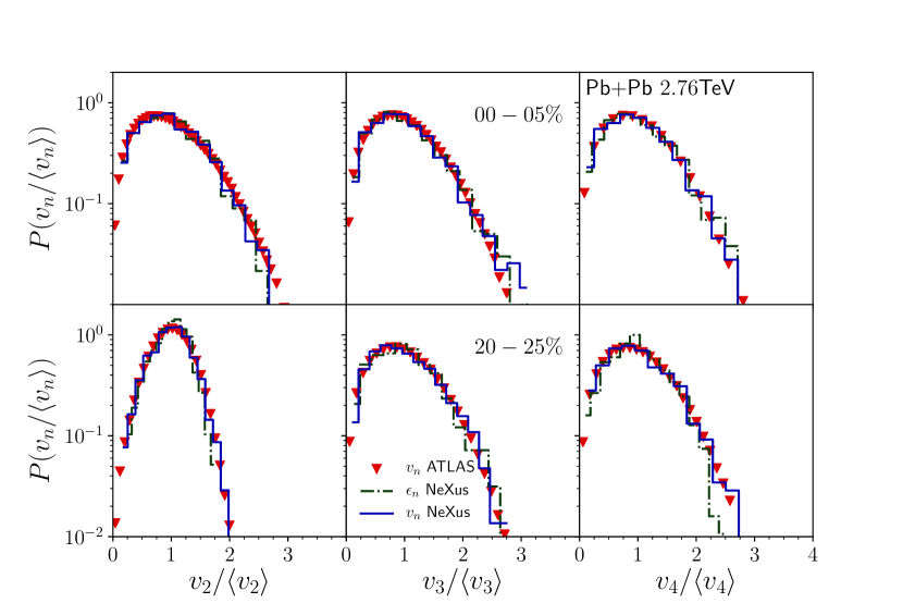
Figure 1: Comparison of scaled $\epsilon_{n}$ and $v_{n}$ distributions from NeXSPheRIO ($|\eta|<2.5$) with ATLAS data ($|\eta|<2.5$) Aad et al. (2013) in the range 0.5 Gev $<p_{t}$ for Pb+Pb collisions at 2.76 TeV. (As expected the right side tail of the scaled $\epsilon_{n}$ may be narrower than the $v_{n}$’s one.)

We now turn to the energy dependence of these distributions: the scaled eccentricity distributions are not expected to depend strongly on the beam energy, so the same should hold for the scaled $v_{n}$ distributions. Predictions for $P(v_{n}/\langle v_{n}\rangle)$ at 5.02 A TeV as well as data and comparison at PbPb 2.76 TeV were presented for IP-Glasma McDonald et al. (2017), AMPT and TRENTO Zhao et al. (2017). No difference was observed between these two LHC energies in all cases. In figure 2, NeXSPheRIO $v_{n}$ distributions are shown for LHC and top RHIC energies. They are also fairly similar even though the energies are more different. From Fig. 2 we see that RHIC has slightly larger fluctuations than LHC for both $v_{2}$ and $v_{3}$, this is consistent with Alba et al. (2017a); Rao et al. (2021) which showed that $v_{2}\left\{4\right\}/v_{2}\left\{2\right\}$ is smaller at RHIC than the LHC (implying that fluctuations are larger at RHIC).

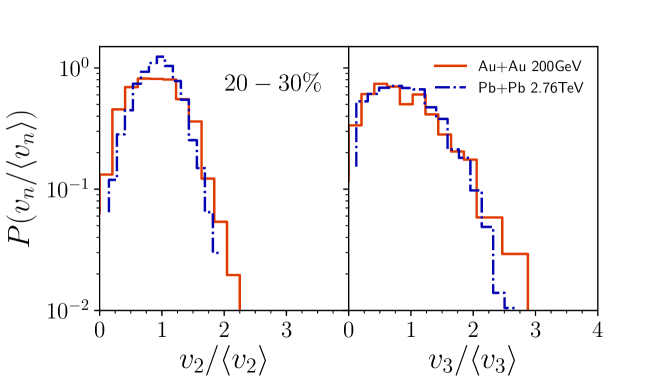
Figure 2: Comparison of scaled $v_{n}$ distributions for NeXSPheRIO ($|\eta|<2.5$) at LHC and RHIC energies for the 20-30% centrality window and 0.5 GeV $<p_{t}$ in the case of Pb+Pb collisions at 2.76 TeV.

Finally, predictions for scaled $v_{n}$ distributions in Au+Au collisions at 200 GeV at various centralities are shown in fig. 3 and 4, comparing TRENTO and NeXus. Unsurprisingly, they are relatively equivalent but we do find that there are some subtle differences in their centrality dependence. TRENTO appears to have fewer fluctuations in central collisions compared to NeXus for both $v_{2}$ and $v_{3}$. Additionally, for $v_{2}$ in peripheral collisions it appears to be reversed in that NeXus then has slightly narrower fluctuations than TRENTO.

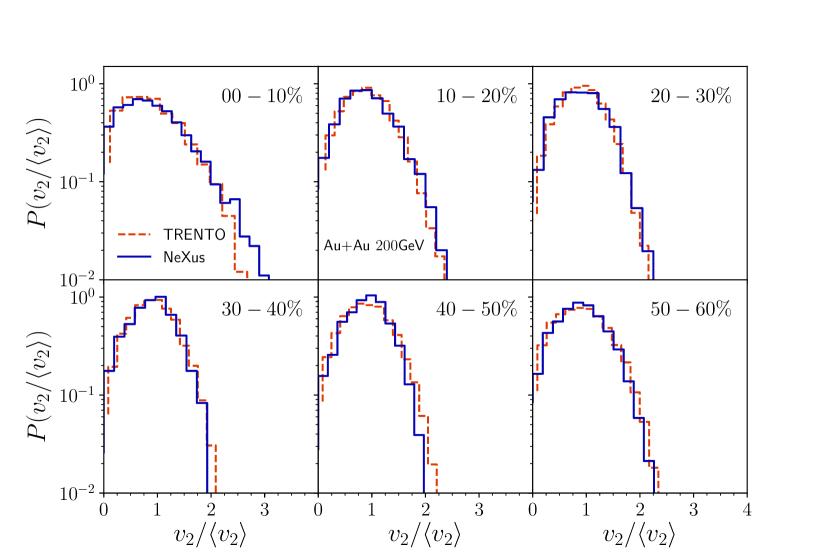
Figure 3: Predictions for scaled $v_{2}$ distributions for NeXus and TRENTO initial conditions for Au+Au collisions at 200 GeV.

Figure 4: Same as figure 3 for $v_{3}$.

We now turn to the flow factorization ratios. As mentioned in Sec. II.2, compared to CMS data Khachatryan et al. (2015), TRENTO provides good results for $r_{2}$ in all centralities but $r_{3}$ exhibits a too large drop for all trigger $p_{T}$’s and centralities Zhao et al. (2017). As can be seen in Fig. 5, similar results hold for NeXus. This effect is more pronounced in central collisions, which also happens to coincide with the $v_{2}$ to $v_{3}$ puzzle Luzum and Ollitrault (2013); CMS (2012); Shen et al. (2015); Rose et al. (2014); Gelis et al. (2019); Carzon et al. (2020); Zakharov (2020). Additionally, it also appears that our theoretical calculations demonstrate the largest suppression compared to the data when $p_{T}^{(a)}$ is large. This may indicate some physical mechanism that is suppressing sources of fluctuations and is not yet included in our simulations plays a role at higher $p_{T}$. Even for mid-central collisions we find a similar discrepancy for $r_{3}$, however, the deviation is significantly smaller.

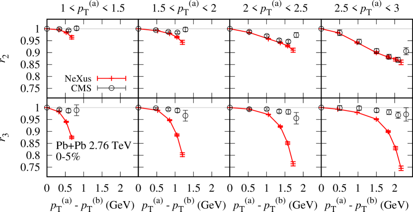
Figure 5: Comparison of $r_{n}$ from NeXSPheRIO ($|\eta|<2.5$) with CMS data Khachatryan et al. (2015) ($|\eta|<2.4$) for Pb+Pb collisions at 2.76 TeV.

We can address the energy dependence of these ratios. Predictions for $r_{n}$ at PbPb 5.02 TeV as well as data and comparison at 2.76 TeV were presented for IP-Glasma McDonald et al. (2017), AMPT and TRENTO Zhao et al. (2017). Some difference was observed between these two LHC energies with a tendency towards more factorization breaking at lower energy. A comparison of factorization breaking for LHC and RHIC energies with TRENTO initial conditions is shown in Figs. 6 and 7. Factorization breaking is always larger at RHIC than at LHC, for $r_{2}$ (less for $r_{3}$) up to 40% centrality. For less central collisions, it becomes smaller than at LHC. Generally, central collisions at higher $p_{T}$ appear to have the largest factorization breaking. However, we note that this is precisely the regime where our predictions struggle to reproduce experimental results so this regime still requires more theoretical effort.

We note also that $r_{3}$ has a much weaker centrality dependence compared to $r_{2}$, which is likely due to the fact that $v_{2}$ also has a geometrical component to it when one varies centrality whereas $v_{3}$ is entirely fluctuations driven. Because $v_{3}$ is primarily driven by fluctuations, which exist regardless of the centrality class then it is not surprising that there is not a strong centrality dependence.

Next we compare central NeXus initial conditions between RHIC and the LHC. A larger breaking is seen at RHIC than at LHC for $r_{2}$ (and not for $r_{3}$) in Fig. 8, which is very similar to what we found for the TRENTO results in Figs. 6-7. We note, however, that the difference in $r_{2}$ for higher $p_{T}$ demonstrates a smaller difference between RHIC and LHC compared to what was seen for the TRENTO intial conditions. Thus, it would be interesting to have factorization breaking measurements from RHIC to further distinguish between initial state models.

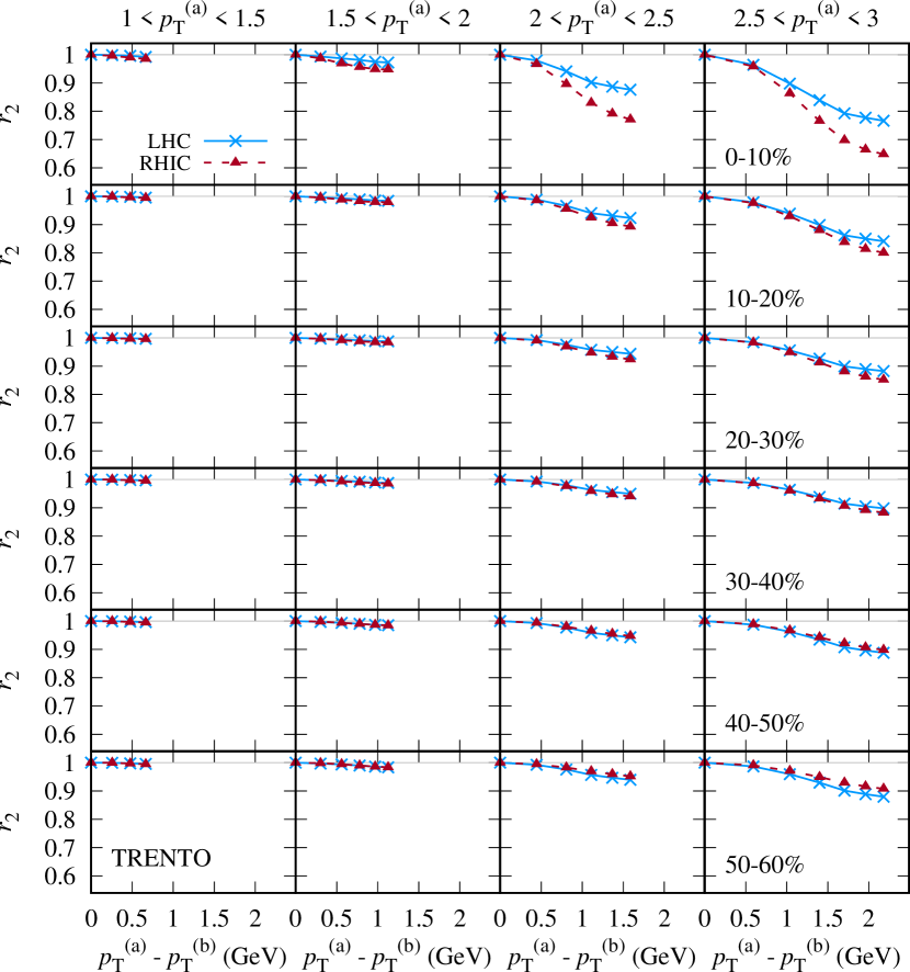
Figure 6: Comparison of $r_{2}$ for Trento at LHC and RHIC energies for various centrality windows.

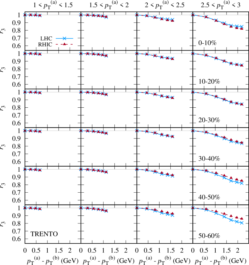
Figure 7: Comparison of $r_{3}$ for Trento at LHC and RHIC energies for various centrality windows.

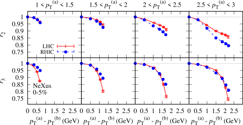
Figure 8: Comparison of $r_{n}$ for NeXSPheRIO ($|\eta|<2.5$) at LHC and RHIC energies for the 0-5% centrality window.

In order to understand how higher energies imply smaller breaking of factorization, we have selected 600 events in a central window and solved the ideal hydrodynamic equations at RHIC. Then exactly the same events had their energy density scaled by a factor of 5, and the hydrodynamic equations were solved. The results shown in Fig. 9, indicate that the factorization breaking for $n=2$ (and less for $n=3$) is stronger at RHIC and this appears to be directly connected to the overall energy density scale, which leads to a longer lifetime at RHIC vs. the LHC. Thus, one can argue that at high-energies due to the longer lifetime of hydrodynamics, one would expect $r_{n}\rightarrow 1$.

To see which part of the flow vector was more affected, the following quantities (for $p_{T}^{(a)}=2.5\,GeV$) were computed:

$$r_{vn}=\langle v_{n}(p_{T}^{(a)})v_{n}(p_{T}^{(b)})\rangle/\sqrt{\langle v_{n}^{2}(p_{T}^{(a)})\rangle\langle v_{n}^{2}(p_{T}^{(b)})\rangle}$$ (6)

and

$$r_{\psi n}=\langle\cos n(\psi_{n}(p_{T}^{(a)})-\psi_{n}(p_{T}^{(b)}))\rangle.$$ (7)

Eq. (6) is a Pearson coefficient between different $p_{T}$ bins of the flow harmonics and Eq. 7 demonstrates the decorrelation of event plane angles across $p_{T}$. Note similar studies have been performed in Betz et al. (2017) to study high $p_{T}$ flow harmonics.

Although these quantities are not independent and their product is not exactly $r_{n}$, we expect that their individual behaviors can help to understand the physical picture. In Fig. 9, the $r_{v_{n}}$ curves are seen to be almost energy independent, while the $r_{\psi_{n}}$ ones are energy dependent. The energy independence of $r_{v_{n}}$ implies that the magnitude of the $v_{n}$’s vs. $p_{T}$ generally scales in the same way regardless of the beam energy. The $r_{\psi_{n}}$ can be understood, since longer lifetimes (LHC energy) lead to different event planes tending to have the same direction due to pressure gradients in the hydrodynamic expansion. The longer that one runs hydrodynamics, the more the event plane angles are aligned.

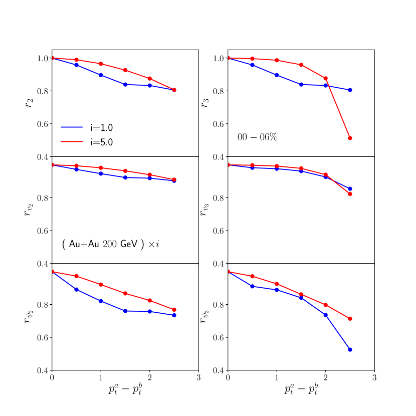
Figure 9: Comparison of factorization breaking for initial conditions at RHIC top energy and the same initial conditions with energy density multiplied by a factor 5. Top row: $r_{2}$ and $r_{3}$, middle row:$r_{v2}$ and $r_{v3}$, bottom row: $r_{\psi 2}$ and $r_{\psi 3}$ (definitions in text). $p_{T}^{(a)}=2.5\,GeV$.

Now that we have better understood the scaling of the factorization with beam energy and subtle differences betwen Trento and NeXus initial conditions, we present the predictions of the factorization breaking ratios at RHIC for TRENTO and NeXus in Fig.s 10-11. We find that for $r_{2}$ low $p_{T}$ values are nearly identical, it is only for $p_{T}^{(a)}$ in bins above $p_{T}^{(a)}>2$ GeV that one can distinguish between TRENTO and NeXus. Additionally, we find that high $p_{T}^{(a)}$ in central collisions is by far the most important region to distinguish between different types of initial conditions.

Comparing our results for both $r_{2}$ ad $r_{3}$ we find that $r_{2}$ also is a better candidate for distinguishing initial state models. While subtle differences exist for $r_{3}$ for TRENTO vs. NeXus in Fig. 11, they would require much more precise experimental data to distinguish between models.

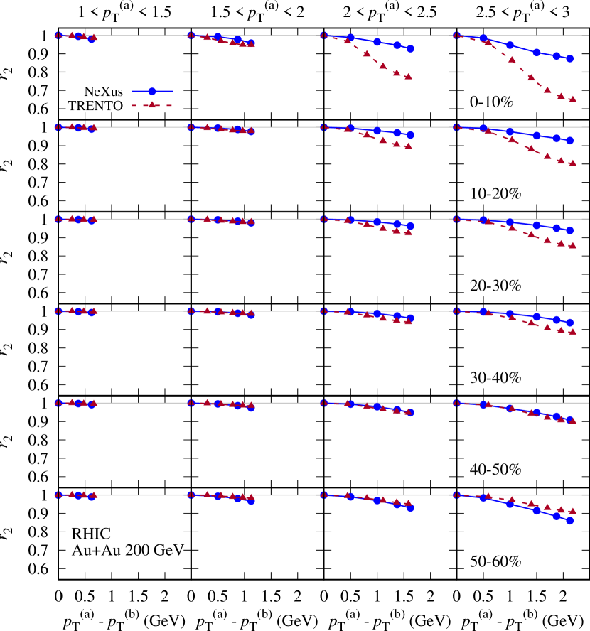
Figure 10: Predictions for $r_{2}$ for NeXus and TRENTO models for Au+Au collisions at 200 A GeV.

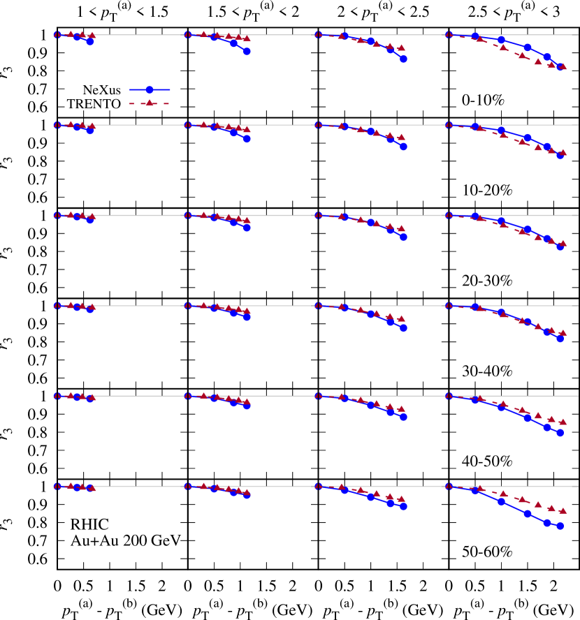
Figure 11: Predictions for $r_{3}$ for NeXus and TRENTO models for Au+Au collisions at 200 A GeV.

V Conclusion

Because RHIC also is more sensitive to a variety of medium effects compared to the LHC (i.e. the finite $\mu_{B}$ equation of state, diffusion, criticality etc), it is that much more important to find medium independent observables that can help to constrain initial state effects. In this paper we concentrate on two quantities that are not very sensitive to viscosity and compare predictions from two initial condition models, NeXus and TRENTO (with $p=0$ configuration). We found that the scaled $v_{n}$ distributions that were used to rule out initial condition models at the LHC do not provide new constraints at top RHIC energy. Here we argue that factorization breaking will be sensitive to the choice in the initial state at RHIC and outline the best centrality and $p_{T}$ windows to study. Generally, we find that $r_{2}$ is a better candidate for distinguishing initial state models and specifically in central collisions and using higher $p_{T}$ cuts.

Our main conclusions that we have found from the factorization breaking ratios, $r_{n}$, is that they seem to be an excellent tool to constrain initial condition models at top RHIC energy: 1) models that lead to fairly similar results at the LHC have very different predictions for RHIC, 2) factorization breaking can be substantially stronger at RHIC (for central collisions). In a previous paper Gardim et al. (2018), we argued that smearing the initial hot spots (without altering large scale structure) has little effect on a range of variables (integrated $v_{n}$, scaled $v_{n}$ distributions, normalized symmetric cumulants, event-plane correlations, $p_{T}$ distributions and $v_{n}(p_{T})$) but modifies $r_{n}$. The difference between $r_{n}$’s for NeXus and TRENTO, that have different scales for their initial inhomogeneities, are a nice illustration of this.

In order to better understand how the factorization breaking observable scales with beam energy, we have calculated two new quantities that correlate either the magnitude of flow harmonics across $p_{T}$, $r_{vn}$, or the correlation between event-plane angles across $p_{T}$, $r_{\psi n}$. We found that the correlation between overall magnitudes of flow harmonics is not strongly sensitive to the lifetime of hydrodynamics. In contrast, though, the correlation of event plan angles is more sensitive to the lifetime of the system.

While not done in this initial study, it may be interesting to also calculate the sensitivity of factorization breaking ratios at RHIC for small systems and lower beam energies. We leave this as a potential future work.

VI Acknowledgements

L.B. thanks support from Conselho Nacional de Desenvolvimento Científico e Tecnológico (CNPq). F.G.G. was supported by Conselho Nacional de Desenvolvimento Científico e Tecnológico (CNPq grant 312203/2015-2) and FAPEMIG (grant APQ-02107-16). F.G. acknowledges support from Fundação de Amparo à Pesquisa do Estado de São Paulo (FAPESP grant 2018/24720-6)and project INCT-FNA Proc. No. 464898/2014-5. J.N.H. acknowledges the support from the US-DOE Nuclear Science Grant No. DE-SC0020633. P.I. thanks support from Coordenação de Aperfeiçoamento de Pessoal de Nível Superior (CAPES) and Conselho Nacional de Desenvolvimento Científico e Tecnológico (CNPq grant 142151/2019-0). M.L. acknowledges support from FAPESP projects 2016/24029-6 and 2017/05685-2, and project INCT-FNA Proc. No. 464898/2014-5.

References

- Ratti (2018) C. Ratti, Rept. Prog. Phys. 81, 084301 (2018), arXiv:1804.07810 [hep-lat] .
- Bzdak et al. (2020) A. Bzdak, S. Esumi, V. Koch, J. Liao, M. Stephanov, and N. Xu, Phys. Rept. 853, 1 (2020), arXiv:1906.00936 [nucl-th] .
- Dexheimer et al. (2020) V. Dexheimer, J. Noronha, J. Noronha-Hostler, C. Ratti, and N. Yunes, (2020), arXiv:2010.08834 [nucl-th] .
- Monnai et al. (2021) A. Monnai, B. Schenke, and C. Shen, Int. J. Mod. Phys. A 36, 2130007 (2021), arXiv:2101.11591 [nucl-th] .
- STARcollaboration (2014) STARcollaboration, “Studying the Phase Diagram of QCD Matter at RHIC,” (2014).
- Cebra et al. (2014) D. Cebra, S. G. Brovko, C. E. Flores, B. A. Haag, and J. L. Klay, (2014), arXiv:1408.1369 [nucl-ex] .
- Galatyuk (2014) T. Galatyuk (HADES), Nucl. Phys. A 931, 41 (2014).
- Friese (2006) V. Friese, Nucl. Phys. A 774, 377 (2006).
- Tahir et al. (2005) N. A. Tahir et al., Phys. Rev. Lett. 95, 035001 (2005).
- Lutz et al. (2009) M. F. M. Lutz et al. (PANDA), (2009), arXiv:0903.3905 [hep-ex] .
- Durante et al. (2019) M. Durante et al., Phys. Scripta 94, 033001 (2019), arXiv:1903.05693 [nucl-th] .
- Kekelidze et al. (2017) V. Kekelidze, A. Kovalenko, R. Lednicky, V. Matveev, I. Meshkov, A. Sorin, and G. Trubnikov, Nucl. Phys. A 967, 884 (2017).
- Kekelidze et al. (2016) V. Kekelidze, A. Kovalenko, R. Lednicky, V. Matveev, I. Meshkov, A. Sorin, and G. Trubnikov, Nucl. Phys. A 956, 846 (2016).
- Heinz and Snellings (2013) U. Heinz and R. Snellings, Ann. Rev. Nucl. Part. Sci. 63, 123 (2013), arXiv:1301.2826 .
- Gale et al. (2013a) C. Gale, S. Jeon, and B. Schenke, Int. J. Mod. Phys. A 28, 1340011 (2013a), arXiv:1301.5893 .
- de Souza et al. (2016) R. D. de Souza, T. Koide, and T. Kodama, Prog. Part. Nucl. Phys. 86, 35 (2016), arXiv:1506.03863 .
- (17) S. Jeon and U. Heinz, “Quark gluon plasma 5,” arXiv:1503.03931 .
- Giacalone et al. (2017a) G. Giacalone, J. Noronha-Hostler, and J.-Y. Ollitrault, Phys. Rev. C95, 054910 (2017a), arXiv:1702.01730 [nucl-th] .
- J.Jia (2013) J.Jia (ATLAS collaboration), Nucl. Phys. A 904-905, 421c (2013), arXiv:1209.4232 .
- Aad et al. (2013) G. Aad et al. (ATLAS collaboration), JHEP 1311, 183 (2013), arXiv:1305.2942 .
- A.R.Timmins (2013) A.R.Timmins (ALICE collaboration), J. Phys. Conf. Ser. 446, 012031 (2013), arXiv:1301.6084 .
- Khachatryan et al. (2015) V. Khachatryan et al. (CMS), Phys. Rev. C92, 034911 (2015), arXiv:1503.01692 [nucl-ex] .
- Acharya et al. (2017) S. Acharya et al. (ALICE), JHEP 09, 032 (2017), arXiv:1707.05690 [nucl-ex] .
- Drescher et al. (2001) H. J. Drescher, M. Hladik, S. Ostapchenko, T. Pierog, and K. Werner, Phys. Rept. 350, 93 (2001), arXiv:hep-ph/0007198 .
- Moreland et al. (2015) J. S. Moreland, J. E. Bernhard, and S. A. Bass, Phys. Rev. C92, 011901 (2015), arXiv:1412.4708 [nucl-th] .
- Miller et al. (2007) M. Miller, K. Reygers, S. J. Sanders, and P. Steinberg, Ann.Rev.Nucl.Part.Sci. 57, 205 (2007), arXiv:nucl-ex/0701025 .
- (27) B.Alver, M.Baker, C.Loizides, and P.Steinberg, arXiv:0805.4411 .
- (28) C. Loizides, J. Nagle, and P. Steinberg, arXiv:1408.2549 .
- H.-J.Drescher and Nara (2007) H.-J.Drescher and Y. Nara, Phys. Rev. C 75, 034905 (2007), arXiv:nucl-th/0611017 .
- Renk and Niemi (2014) T. Renk and H. Niemi, Phys. Rev. C89, 064907 (2014), arXiv:1401.2069 [nucl-th] .
- S.Ghosh et al. (2016) S.Ghosh, S. K. Singh, S. Chatterjee, J. Alam, and S. Sarkar, Phys. Rev. C 93, 054904 (2016), arXiv:1601.03971 .
- Schenke et al. (2012) B. Schenke, P. Tribedy, and R. Venugopalan, Phys. Rev. Lett. 108, 252301 (2012), arXiv:1202.6646 .
- McDonald et al. (2017) S. McDonald, C. Shen, F. Fillion-Gourdeau, S. Jeon, and C. Gale, Phys. Rev. C95, 064913 (2017), arXiv:1609.02958 [hep-ph] .
- Gale et al. (2013b) C. Gale, S. Jeon, B. Schenke, P. Tribedy, and R. Venugopalan, Phys. Rev. Lett. 110, 012302 (2013b), arXiv:1209.6330 .
- Eskola et al. (2000) K. J. Eskola, K. Kajantie, P. V. Ruuskanen, and K. Tuominen, Nucl. Phys. B570, 379 (2000), arXiv:hep-ph/9909456 .
- Niemi et al. (2016) H. Niemi, K. J. Eskola, and R. Paatelainen, Phys. Rev. C93, 024907 (2016), arXiv:1505.02677 [hep-ph] .
- Zhang et al. (2000) B. Zhang, C. M. Ko, B.-A. Li, and Z.-w. Lin, Phys. Rev. C61, 067901 (2000), arXiv:nucl-th/9907017 [nucl-th] .
- Zhao et al. (2017) W. Zhao, H.-j. Xu, and H. Song, Eur. Phys. J. C77, 645 (2017), arXiv:1703.10792 [nucl-th] .
- Niemi et al. (2013) H. Niemi, G. S. Denicol, H. Holopainen, and P. Huovinen, Phys. Rev. C 87, 054901 (2013), arXiv:1212.1008 .
- Gardim et al. (2018) F. G. Gardim, F. Grassi, P. Ishida, M. Luzum, P. S. Magalhães, and J. Noronha-Hostler, Phys. Rev. C 97, 064919 (2018), arXiv:1712.03912 [nucl-th] .
- Gardim et al. (2012a) F. G. Gardim, F. Grassi, M. Luzum, and J.-Y. Ollitrault, Phys. Rev. C 85, 024908 (2012a), arXiv:1111.6538 .
- Gardim et al. (2015) F. G. Gardim, J. Noronha-Hostler, M. Luzum, and F. Grassi, Phys. Rev. C 91, 034902 (2015), arXiv:1411.2574 .
- Fu (2015) J. Fu, Phys. Rev. C 92, 024904 (2015).
- Noronha-Hostler et al. (2016a) J. Noronha-Hostler, B. Betz, J. Noronha, and M. Gyulassy, Phys. Rev. Lett. 116, 252301 (2016a), arXiv:1602.03788 [nucl-th] .
- Betz et al. (2017) B. Betz, M. Gyulassy, M. Luzum, J. Noronha, J. Noronha-Hostler, I. Portillo, and C. Ratti, Phys. Rev. C95, 044901 (2017), arXiv:1609.05171 [nucl-th] .
- Prado et al. (2016) C. A. G. Prado, J. Noronha-Hostler, A. A. P. Suaide, J. Noronha, M. G. Munhoz, and M. R. Cosentino, (2016), arXiv:1611.02965 [nucl-th] .
- Katz et al. (2020) R. Katz, C. A. G. Prado, J. Noronha-Hostler, J. Noronha, and A. A. P. Suaide, Phys. Rev. C 102, 024906 (2020), arXiv:1906.10768 [nucl-th] .
- Noronha-Hostler et al. (2016b) J. Noronha-Hostler, L. Yan, F. G. Gardim, and J.-Y. Ollitraul, Phys. Rev. C 93, 014909 (2016b), arXiv:1511.03896 .
- Sievert and Noronha-Hostler (2019) M. D. Sievert and J. Noronha-Hostler, Phys. Rev. C 100, 024904 (2019), arXiv:1901.01319 [nucl-th] .
- Rao et al. (2021) S. Rao, M. Sievert, and J. Noronha-Hostler, Phys. Rev. C 103, 034910 (2021), arXiv:1910.03677 [nucl-th] .
- Hippert et al. (2020) M. Hippert, J. a. G. P. Barbon, D. Dobrigkeit Chinellato, M. Luzum, J. Noronha, T. Nunes da Silva, W. M. Serenone, and J. Takahashi, Phys. Rev. C 102, 064909 (2020), arXiv:2006.13358 [nucl-th] .
- Voloshin et al. (2008) S. A. Voloshin, A. M. Poskanzer, A. Tang, and G. Wang, Phys. Lett. B659, 537 (2008), arXiv:0708.0800 [nucl-th] .
- Yan and Ollitrault (2014) L. Yan and J.-Y. Ollitrault, Phys. Rev. Lett. 112, 082301 (2014), arXiv:1312.6555 .
- Yan et al. (2014) L. Yan, J.-Y. Ollitrault, and A. Poskanzer, Phys. Rev. C 90, 024903 (2014), arXiv:1405.6595 .
- Yan et al. (2015) L. Yan, J.-Y. Ollitrault, and A. Poskanzer, Phys. Lett. B 742, 290 (2015), arXiv:1408.0921 .
- F.Gardim et al. (2012) F.Gardim, F.Grassi, M.Luzum, and J.-Y.Ollitrault, Phys. Rev. C 87, 031901(R) (2012).
- (57) I.Kozlov, M.Luzum, G.Denicol, S. Jeon, and C. Gale, arXiv:1405.3976 .
- U.Heinz et al. (2013) U.Heinz, Z. Qiu, and C. Shen, Phys. Rev. C 87, 034913 (2013).
- Werner (1993) K. Werner, Phys. Rept. 232, 87 (1993).
- Drescher et al. (2002) H. J. Drescher, S. Ostapchenko, T. Pierog, and K. Werner, Phys. Rev. C 65, 054902 (2002), arXiv:hep-ph/0011219 .
- Qian et al. (2007) W. L. Qian, R. Andrade, F. Grassi, J. O. Socolowski, T. Kodama, and Y. Hama, Int. J. Mod. Phys. E 16, 1877 (2007), nucl-th/arXiv:0703078 .
- Andrade et al. (2006) R. P. G. Andrade, F. Grassi, Y. Hama, T. Kodama, and J. O. Socolowski, Phys. Rev. Lett. 97, 202302 (2006), arXiv:nucl-th/0608067 .
- Andrade et al. (2008) R. P. G. Andrade, F. Grassi, Y. Hama, T. Kodama, and W. L. Qian, Phys. Rev. Lett. 101, 112301 (2008), arXiv:0805.0018 .
- Andrade et al. (2009) R. P. G. Andrade, A. dos Reis, F. Grassi, Y. Hama, W. Qian, T. Kodama, and J.-Y. Ollitrault, Acta Phys.Polon.B 40, 993 (2009), arXiv:0812.4143 .
- Gardim et al. (2011) F. G. Gardim, F. Grassi, Y. Hama, M. Luzum, and J. Y. Ollitrault, Phys. Rev. C 83, 064901 (2011), arXiv:1103.4605 .
- Gardim et al. (2012b) F. G. Gardim, F. Grassi, M. Luzum, and J.-Y. Ollitrault, Phys. Rev. Lett. 109, 202302 (2012b), arXiv:1203.2882 .
- Takahashi et al. (2009) J. Takahashi et al., Phys. Rev. Lett. 103, 242301 (2009), arXiv:0902.4870 .
- W.L.Qian et al. (2013) W.L.Qian, R. P. G. Andrade, F. Gardim, F. Grassi, and Y. Hama, Phys. Rev. C 87, 014904 (2013), arXiv:1207.6415 .
- Machado (2015) M. V. Machado, Event-by-event hydrodynamics for the LHC, Master’s thesis, Universidade de São Paulo, Brazil (2015).
- Gardim et al. (2020) F. G. Gardim, F. Grassi, P. Ishida, M. Luzum, and J.-Y. Ollitrault, in 28th International Conference on Ultrarelativistic Nucleus-Nucleus Collisions (2020) arXiv:2002.01747 [nucl-th] .
- Bernhard et al. (2016) J. E. Bernhard, J. S. Moreland, S. A. Bass, J. Liu, and U. Heinz, Phys. Rev. C94, 024907 (2016), arXiv:1605.03954 [nucl-th] .
- Alba et al. (2017a) P. Alba, V. M. Sarti, J. Noronha, J. Noronha-Hostler, P. Parotto, I. P. Vazquez, and C. Ratti, (2017a), arXiv:1711.05207 [nucl-th] .
- Nijs et al. (2020) G. Nijs, W. Van Der Schee, U. Gürsoy, and R. Snellings, (2020), arXiv:2010.15134 [nucl-th] .
- Summerfield et al. (2021) N. Summerfield, B.-N. Lu, C. Plumberg, D. Lee, J. Noronha-Hostler, and A. Timmins, (2021), arXiv:2103.03345 [nucl-th] .
- Ke et al. (2017) W. Ke, J. S. Moreland, J. E. Bernhard, and S. A. Bass, Phys. Rev. C 96, 044912 (2017), arXiv:1610.08490 [nucl-th] .
- Mordasini et al. (2020) C. Mordasini, A. Bilandzic, D. Karakoç, and S. F. Taghavi, Phys. Rev. C 102, 024907 (2020), arXiv:1901.06968 [nucl-ex] .
- Giacalone et al. (2021a) G. Giacalone, F. G. Gardim, J. Noronha-Hostler, and J.-Y. Ollitrault, Phys. Rev. C 103, 024910 (2021a), arXiv:2004.09799 [nucl-th] .
- Giacalone et al. (2021b) G. Giacalone, F. G. Gardim, J. Noronha-Hostler, and J.-Y. Ollitrault, Phys. Rev. C 103, 024909 (2021b), arXiv:2004.01765 [nucl-th] .
- ATLAS (2021) ATLAS, “Measurement of flow and transverse momentum correlations in Pb+Pb collisions at TeV and Xe+Xe collisions at TeV with the ATLAS detector,” (2021).
- Aguiar et al. (2001) C. Aguiar, T. Kodama, T. Osada, and Y. Hama, J.Phys.G 27, 75 (2001), arXiv:hep-ph/0006239 .
- Hama et al. (2006) Y. Hama, R. P. Andrade, F. Grassi, O. S. Jr, T. Kodama, B. Tavares, and S. S. Padula, Nucl.Phys.A 169, 774 (2006), arXiv:hep-ph/0510096 .
- Noronha-Hostler et al. (2013) J. Noronha-Hostler, G. S. Denicol, J. Noronha, R. P. G. Andrade, and F. Grassi, Phys. Rev. C 88, 044916 (2013), arXiv:1305.1981 .
- Noronha-Hostler et al. (2014) J. Noronha-Hostler, J. Noronha, and F. Grassi, Phys. Rev. C 90, 034907 (2014), arXiv:1406.3333 .
- Alba et al. (2017b) P. Alba et al., Phys. Rev. D 96, 034517 (2017b), arXiv:1702.01113 [hep-lat] .
- Giacalone et al. (2017b) G. Giacalone, L. Yan, J. Noronha-Hostler, and J.-Y. Ollitrault, J. Phys. Conf. Ser. 779, 012064 (2017b), arXiv:1608.06022 [nucl-th] .
- Luzum and Ollitrault (2013) M. Luzum and J.-Y. Ollitrault, Nucl. Phys. A 904-905, 377c (2013), arXiv:1210.6010 [nucl-th] .
- CMS (2012) CMS, “Azimuthal anisotropy harmonics in ultra-central PbPb collisions at sqrts_NN = 2.76 TeV,” (2012).
- Shen et al. (2015) C. Shen, Z. Qiu, and U. Heinz, Phys. Rev. C92, 014901 (2015), arXiv:1502.04636 [nucl-th] .
- Rose et al. (2014) J.-B. Rose, J.-F. Paquet, G. S. Denicol, M. Luzum, B. Schenke, S. Jeon, and C. Gale, Nucl. Phys. A 931, 926 (2014), arXiv:1408.0024 [nucl-th] .
- Gelis et al. (2019) F. Gelis, G. Giacalone, P. Guerrero-Rodríguez, C. Marquet, and J.-Y. Ollitrault, (2019), arXiv:1907.10948 [nucl-th] .
- Carzon et al. (2020) P. Carzon, S. Rao, M. Luzum, M. Sievert, and J. Noronha-Hostler, Phys. Rev. C 102, 054905 (2020), arXiv:2007.00780 [nucl-th] .
- Zakharov (2020) B. G. Zakharov, JETP Lett. 112, 393 (2020), arXiv:2008.07304 [nucl-th] .