TIC 454140642: A Compact, Coplanar, Quadruple-lined Quadruple Star System Consisting of Two Eclipsing Binaries

Abstract

We report the discovery of a compact, coplanar, quadruply-lined, eclipsing quadruple star system from TESS data, TIC 454140642, also known as TYC 0074-01254-1. The target was first detected in Sector 5 with 30-min cadence in Full-Frame Images and then observed in Sector 32 with 2-min cadence. The light curve exhibits two sets of primary and secondary eclipses with periods of $\rm P_{A}=13.624$ days (binary A) and $\rm P_{B}=10.393$ days (binary B). Analysis of archival and follow-up data shows clear eclipse-timing variations and divergent radial velocities, indicating dynamical interactions between the two binaries and confirming that they form a gravitationally-bound quadruple system with a 2+2 hierarchy. The Aa+Ab binary, Ba+Bb binary, and A-B system are aligned with respect to each other within a fraction of a degree: the respective mutual orbital inclinations are 0.25 degrees (A vs B), 0.37 degrees (A vs A-B), and 0.47 degrees (B vs A-B). The A-B system has an orbital period of 432 days – the second shortest amongst confirmed quadruple systems – and an orbital eccentricity of 0.3.

1 Introduction

A few percent of F- and G-type stars are members of stellar quadruples, and the fraction likely increases with stellar mass (e.g Raghavan et al., 2010; De Rosa et al., 2014; Toonen et al., 2016; Moe & Di Stefano, 2017; Tokovinin, 2017). These systems are ideal laboratories to study stellar formation and evolution in a dynamically-complex environment where the constituent binary stars can be close enough to interact with each other. These interactions can occur multiple times over the lifetime of the system, involve e.g. Lidov-Kozai oscillations (Lidov 1962; Kozai 1962; Pejcha et al. 2013), mass-transfer, tidal and dynamical interactions, mergers (Perets & Fabrycky 2009, Hammers et al. 2021), or formation of tight binaries (e.g. Naoz & Fabrycky 2014, and references therein). Quadruple systems are important participants in stellar evolution as a potential source for Type I SNe (Fang et al. 2018), as well as interesting outcomes such as common-envelope evolution, interactions with circumbinary disks, etc.

Detection and detailed characterization of a bona-fide quadruple-star system can be challenging. For example, it is not uncommon for close eclipsing binary stars to exhibit deviations from strict periodicity and recent studies show that at least $\sim 7\%$ of Kepler’s eclipsing binary stars show such deviations within the 4-year-long observing window of the Kepler prime mission (e.g. Rappaport et al. 2013, Orosz 2015, Borkovits et al. 2016). Such eclipse timing variations (ETVs) can be indicative of dynamical interactions between the eclipsing binary and additional star(s) on wider orbit(s), and provide an important detection method for triple, quadruple, and higher-order stellar systems, as well as for circumbinary planets (e.g. Borkovits et al. 2016, Welsh & Orosz 2018). Other pathways for the detection of quadruple (and higher-order multiples) are visual and spectroscopic observations (e.g. Raghavan et al. 2010, Tokovinin 2017, Pribulla et al. 2006), but these methods generally do not guarantee that the potentially additional star(s) are indeed gravitationally-bound to the known binary.

A target star exhibiting multiple sets of eclipses, ETVs, and per-EB divergent radial velocities provides a unique opportunity to not only confirm the multiplicity of the system but also measure the orbital and physical parameters of its constituents with exquisite precision (e.g. Carter et al. 2011; Borkovits et al. 2018, 2020a, 2021). We note that because the outer orbital period of quadruple systems is much longer than the periods of the inner binaries (for otherwise the system would become unstable), detecting such features requires continuous and long-baseline observations of the target. A combination of space-based photometric surveys, extensive ground-based surveys photometry, and dedicated spectroscopy follow-up is ideally-suited to provide such observations. This was demonstrated by the highly-successful Kepler mission which detected a number of EB systems exhibiting additional features indicative of either circumbinary planets or triple and higher-order stellar systems (e.g. Welsh & Orosz 2018; Kirk et al. 2015, Borkovits et al. 2016).

The Transiting Exoplanet Survey Satellite (TESS, Ricker et al. 2015) is equally capable of discovering multiply-eclipsing stellar systems, as already demonstrated by Borkovits et al. (2020b, 2021) for stellar triples and quadruples, and Powell et al. (2021) for sextuples. The target presented here, TIC 454140642, exhibits the typical 2+2 hierarchy for quadruple systems, illustrated in Fig. 1, and joins the small number of such confirmed, well-characterized systems — VW LMi (Pribulla et al., 2008), V994 Her (Zasche & Uhlař, 2016), V482 Per (Torres et al. 2017), EPIC 220204960 (Rappaport et al., 2017), EPIC 219217635 (Borkovits et al., 2018), CzeV1731 (Zasche et al., 2020), TIC 278956474 (Rowden et al., 2020), and BG Ind (Borkovits et al., 2021).

We note that while quadruple star systems have lower occurrence rates compared to triple systems, the larger outer orbit necessary for stability in the latter systems is generally well beyond the 27-day TESS observation time in a single sector. Specifically, the long outer orbital period substantially reduces the probability that tertiary eclipses or occultations of a stellar triple will be identified in one sector of TESS data. While such triples can (and do) produce multiple tertiary eclipses or occultations during one conjunction of the outer orbit in a singe sector of TESS data (e.g. Borkovits et al., 2020b), detecting multiple such conjunctions in one sector of data is highly unlikely. In turn, this makes determining the outer period of such triples – and thus the overall configuration of the respective system – challenging. In contrast, quadruple systems do not need to be at a conjunction of the outer orbit to reveal their nature, and eclipses/occultations of their constituent binaries can (and do) easily occur in a single sector of TESS data.

Here we present the discovery of the quadruple star TIC 454140642 that exhibits four sets of eclipses as well as prominent, dynamically induced apsidal motion, and short-term four-body perturbations. At the time of writing, TIC 454140642 is the closest to coplanarity amongst the quadruple systems mentioned above, and has the second shortest outer period (after VW LMi). This paper is organized as follows. Section 2 outlines the detection of the target in TESS data. In Sections 3 and 4 we describe the analysis of the available archival data and our follow-up observations, respectively. In Section 5 we present our comprehensive spectro-photodynamical analysis of the system’s parameters. We discuss the properties of the system in Section 6 and draw our conclusions in Section 7.

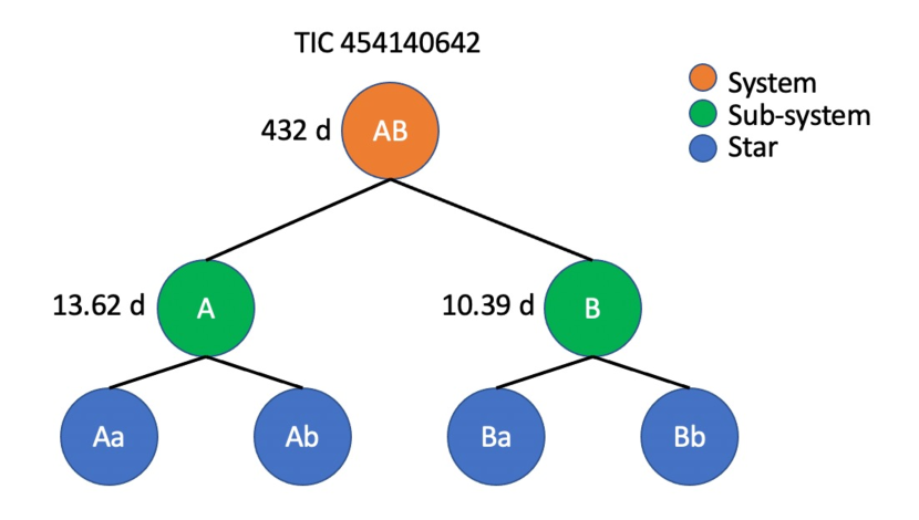
Figure 1: Structure of TIC 454140642, a quadruple star system consisting of two eclipsing binaries.

2 Detection

Our detection methodology is described in detail by Powell et al. (2021). Briefly, we found hundreds of thousands of eclipsing binaries using a neural network classifier on the TESS Full-Frame Image (FFI) light curves. Through manual examination of the lightcurves identified by the neural network as EBs, we found many that showed eclipses belonging to multiple periods in the same light curve. Through photocenter analysis, we determined that the large majority of these lightcurves are consistent with a superposition of two EBs originating from unrelated target stars within the same TESS aperture. A fraction of these, however, demonstrated on-target photocenter for all detected eclipses, suggesting they originate from the same stellar system.

TIC 454140642, a previously unknown EB, was one of the systems that we found early in our examination of TESS light curves. The nature of the system was initially quite challenging to decipher because all the eclipses are similar in depth and duration, in addition to the fact we only had one sector of data with each eclipse present twice in the lightcurve. Preliminary analysis indicated that there are two sets of primary and secondary eclipses. The TESS eleanor lightcurve (Feinstein et al., 2019) for Sectors 5 and 32 is shown in Fig. 2, highlighting the four sets of eclipses; there are no visible out-of-eclipse variations. In accordance with the designation system developed by the IAU, these binaries will be referred to as A (the brighter one with a period of 13.62 days, and components Aa and Ab) and B (the fainter one, with a period of 10.39 days and components Ba and Bb). The contamination due to nearby sources is low according to the TESS Input Catalog (0.001), and photocenter analysis confirmed that both sets of eclipses originate from the target (see Fig. 3), indicating a potential quadruple system. This motivated us to submit the target for 2-min cadence observations in Sector 32 (TESS DDT program 020 PI: Kostov), and also coordinate follow-up efforts with the TESS Follow-up Observing Program (TFOP). The parameters of the system are listed in Table 1.

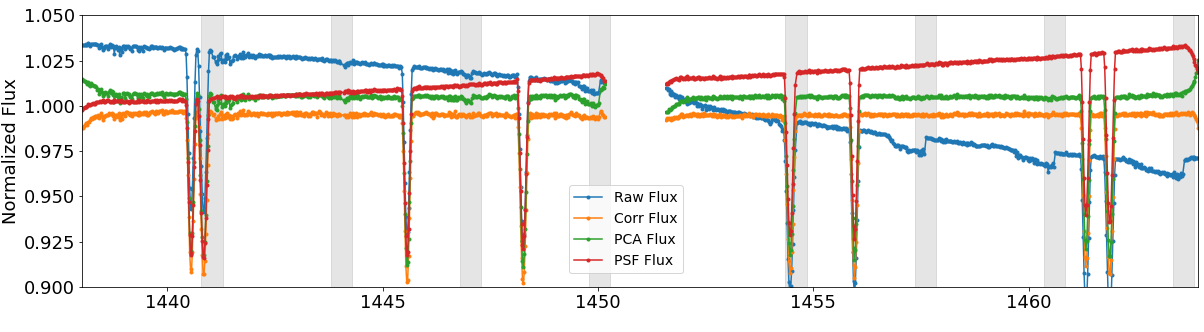
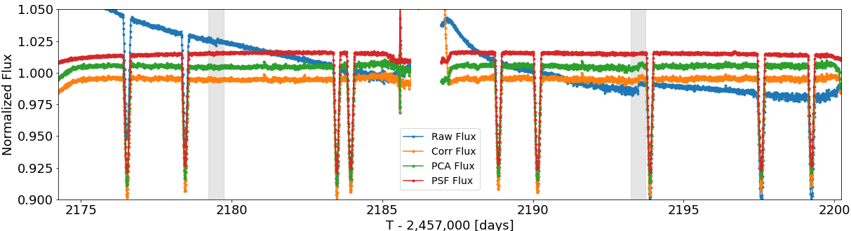
Figure 2: TESS photometry of TIC 454140642, constructed using eleanor (Feinstein et al., 2019), showing the raw flux (blue), corrected flux (orange), PCA flux (green), and PSF flux (red) lightcurve. The eclipses are present in all four lightcurves and are not strongly affected by known systematics such as momentum dumps (vertical grey bands) or background artifacts (spike near 2185.5). The upper panel shows Sector 5 data, the lower panel shows Sector 32 data. There are no apparent out-of-eclipse variations.

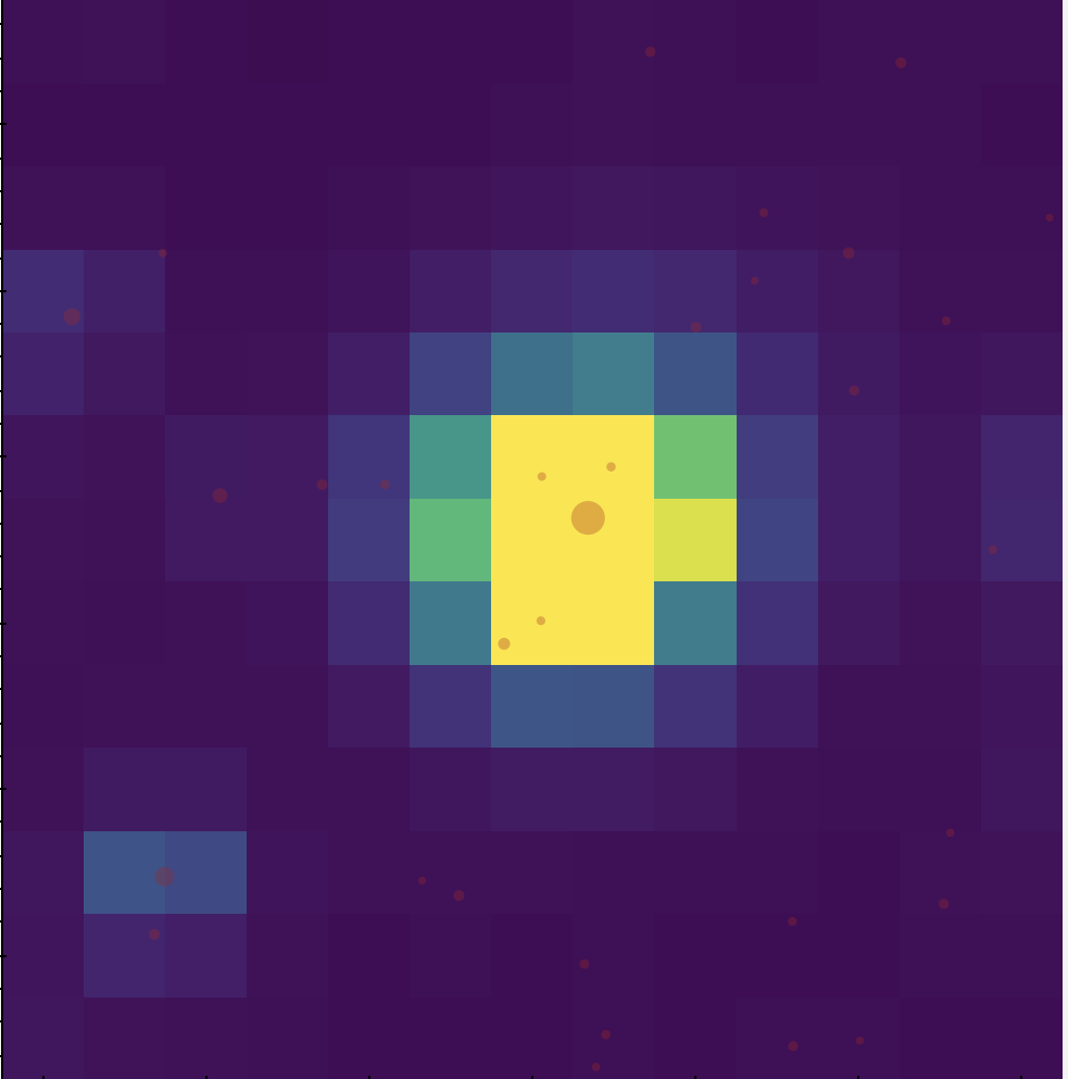
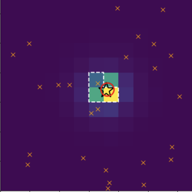
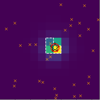
Figure 3: Left: TESS aperture image of TIC 454140642 ($T=9.855$ mag) overlaid with Skyview sources brighter than $T=21$ mag. Center: Mean difference image (out-of-eclipse minus in-eclipse) showing the measured average center-of-light of binary A eclipses (large red symbol), and the catalog position of the target (black star). Right: same as the left panel but for the binary B eclipses. All four sets of eclipses are on-target. The orange crosses represent nearby stars within ${\rm\Delta T=10~{}mag}$.

Table 1: Stellar parameters for TIC 454140642

Parameter	Value	Error	Source
Identifying Information
TIC ID	454140642		1
Gaia ID	3255659981455492608		2
Tycho Reference ID	0074-01254-1		3
$\alpha$ (J2000, hh:mm:ss)	4:19:05.63		2
$\delta$ (J2000, dd:mm:ss)	+00:54:00.2		2
$\mu_{\alpha}$ (mas yr-1)	$2.539$	0.023	2
$\mu_{\delta}$ (mas yr-1)	$-10.670$	0.018	2
$\varpi$ (mas)	2.7864	0.0215	2
Distance (pc)	358.8893	0.0407	2
Photometric Properties
$T$ (mag)	9.8549	0.0097	1
$B$ (mag)	10.945	0.111	4
$V$ (mag)	10.409	0.008	1
$Gaia$ (mag)	10.2224	0.0028	2
$G_{BP}$ (mag)	10.49970	0.001265	2
$G_{RP}$ (mag)	9.80662	0.001475	2
$B_{T}$ (mag)	10.769	0.058	3
$V_{T}$ (mag)	10.329	0.063	3
$g^{\prime}$ (mag)	10.613	0.098	4
$r^{\prime}$ (mag)	10.229	0.041	4
$i^{\prime}$ (mag)	10.123	0.021	4
$J$ (mag)	9.349	0.027	5
$H$ (mag)	9.116	0.026	5
$K$ (mag)	9.022	0.019	5
$W1$ (mag)	9.010	0.023	6
$W2$ (mag)	9.036	0.020	6
$W3$ (mag)	9.046	0.032	6
$W4$ (mag)	8.431	0.028	6
$FUV$ (mag)	18.381	0.195	7
$NUV$ (mag)	12.771	0.007	7
Contamination	0.0014		1
Stellar Properties
Teff, Aa (K)	6434	30	This work
Teff, Ab (K)	6303	30	This work
Teff, Ba (K)	6303	30	This work
Teff, Bb (K)	6188	35	This work
$[$Fe/H$]$	-0.039	0.022	This work
Age (Gyr)	1.945	.27	This work

Sources: (1) TIC-8 (Stassun et al., 2018), (2) Gaia EDR3 (Gaia Collaboration et al., 2020), (3) Tycho-2 catalog (Høg et al., 2000), (4) APASS DR9 (Henden et al., 2015), (5) 2MASS All-Sky Catalog of Point Sources (Skrutskie et al., 2006), (6) AllWISE catalog (Cutri et al., 2012), (7) GALEX-DR5 (GR5) (Bianchi et al., 2011)

3 Photometric data

There is extensive archival data on TIC 454140642 from the WASP and ASAS-SN surveys (Pollacco et al. 2006, Shappee et al. 2014, Kochanek et al. 2017), altogether covering more than 4000 days. The time span of the available photometric data is shown in Figure 4, which includes the TESS data as well as our follow-up photometry.

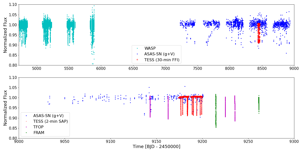
Figure 4: Photometry of the target from ASAS-SN (blue symbols for both g-filter and V-filter), FRAM (green symbols), TESS (red symbols), TFOP (magenta symbols), and WASP 200-mm lenses (cyan symbols), highlighting the covered baseline.

The ASAS-SN data of TIC 454140642 provide coverage of about 2000 days and overlap with TESS data. The target was observed by WASP with both the 85-mm and the 200-mm lenses, although the SNR of the former is poor and thus for our analysis we use only the latter. All four sets of eclipses are clearly recovered in the ASAS-SN and WASP data as shown in Figure 5. Box Least Squares” analysis (BLS, Kovács et al. 2002) analysis of the two datasets provides similar orbital periods for the two binaries, as indicated in the figure captions and listed in Table 2. We note that the periods listed in the table are derived from the photometry alone; the final orbital periods are derived from the comprehensive spectro-photodynamical model described in Section 5.1. Altogether, the available photometry phase-folded on the periods listed in Table 2 shows clear apsidal motion (see Fig. 6) and indicates dynamical interactions between the two binaries.

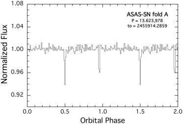
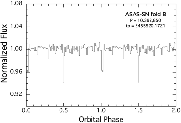
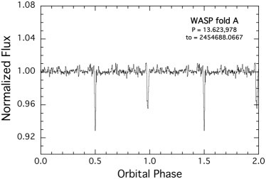
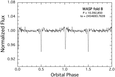
Figure 5: Folds of the ASAS-SN (top) and WASP (bottom) archival data for the two binaries about their respective orbital periods.

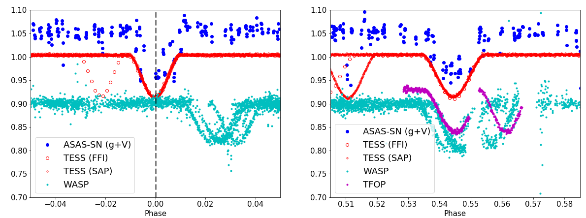
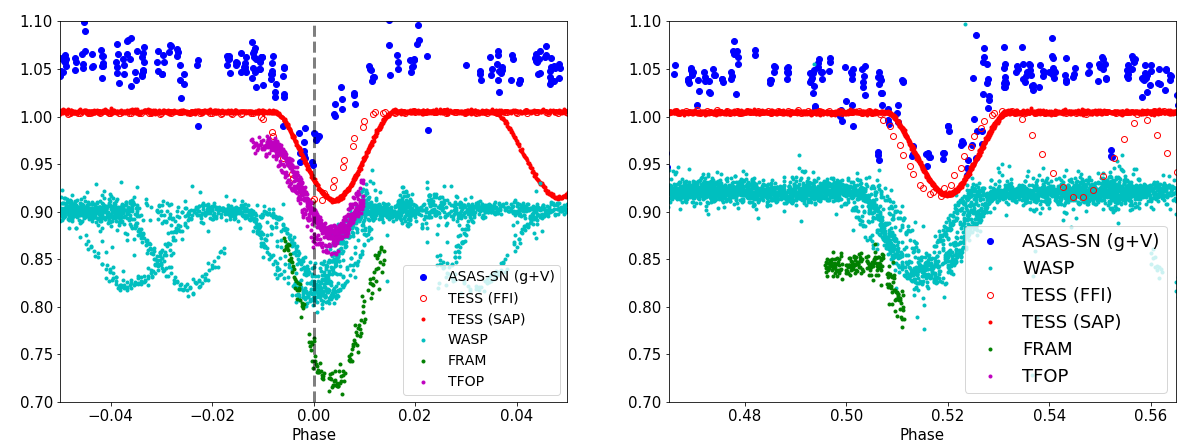
Figure 6: Upper panels: Phase-folded lightcurve of TIC 454140642 for the primary (left) and secondary (right) eclipses of Binary A (using the global fitted ephemerides from Table 2), highlighting the prominent apsidal motion. The different datasets are vertically offset for clarity. Lower panels: Same as above but for Binary B.

Table 2: Derived ephemerides for the two EBs in TIC 454140642 from ASAS-SN, TESS, and WASP data.

Binary	A		B
${\bf ASAS-SN}$
Period [days]	13.623978		10.392850
T0 [BJD - 2450000]	5914.2859		5920.1721
${\bf TESS}$
Period [days]	13.62395		10.39335
T0 [BJD - 2450000]	8440.8394		8445.5638
${\bf WASP}$
Period [days]	13.623978		10.392850
T0 [BJD - 2450000]	4694.1464		4693.7639
Global Fitted Periods	13.6239		10.3928
Global Fitted T0 [BJD - 2450000]	8454.4688		8445.5610

4 Follow-up observations

4.1 Spectroscopy

TIC 454140642 was monitored spectroscopically with the Tillinghast Reflector Echelle Spectrograph (TRES; Szentgyorgyi & Furész, 2007; Fürész, 2008) mounted on the 1.5m Tillinghast reflector at the Fred L. Whipple Observatory on Mount Hopkins (AZ). TRES is a bench-mounted, fiber-fed instrument with a resolving power of $R\simeq 44,000$, and a wavelength coverage of 3900–9100 Å in 51 orders. In total we gathered 26 spectra between September of 2020 and February of 2021, with signal-to-noise ratios in the region of the Mg I b triplet ($\sim$5185 Å) ranging from 28 to 60 per resolution element of 6.8 km s^-1. Exposure times ranged between 450 and 2400 seconds. The spectra were extracted and reduced as per Buchhave et al. (2010), with wavelength solutions derived from bracketing thorium-argon lamp exposures.

The very first spectrum of TIC 454140642 showed four sets of lines, which we expected should represent the two components of two double-lined binaries in the system (see Figure 7). Radial velocities were measured using QUADCOR, a four-dimensional cross-correlation algorithm introduced by Torres et al. (2007), which uses four separate and possibly different templates matched to each star. In this case, however, the stars turn out to be quite similar to each other (see below), so we adopted the same template for the four components. We used a synthetic spectrum taken from a large library of calculated spectra based on model atmospheres by R. L. Kurucz (see Nordstroem et al., 1994; Latham et al., 2002), covering the region of the Mg I b triplet. The template parameters were $T_{\rm eff}=6250$ K, $\log g=4.5$, ${\rm[m/H]}=0.0$, and no rotational broadening. The choice of zero rotational broadening was based on experiments with a range of values for $v\sin i$, which indicated the broadening for all four stars is smaller than our spectral resolution. In addition to the velocities, we used QUADCOR to measure the flux ratios among the components at the mean wavelength of our observations.

Figure 7: Sample 1-D cross-correlation functions for TIC 454140642 showing resolved peaks for the four components.

While approximate orbital periods were known from the photometry for the two binaries undergoing eclipses, at first it was not trivial to identify which set of lines corresponded to which component of which binary. In several of the spectra the lines were heavily blended, so the velocity determinations were not always possible for all four stars at this early stage, and were guided by the location of the peaks in plots of the one-dimensional cross-correlation functions. The process was further complicated by the degeneracy between the flux ratios and the velocity separations when the lines are blended, which made the velocities imprecise. Based on the more reliable flux ratios from the relatively few spectra with well separated lines, it was eventually realized that one star was brighter than the other three, another was the faintest, and the remaining two had similar brightness. Gathering the velocities for the brighter and fainter components, and sorting out the others based on the preliminary photometric ephemerides, we obtained initial orbital solutions for the two binaries based on the 18 observations through mid-December 2020. These fits showed considerable scatter, far in excess of the precision expected for the measurements. The primary and secondary residuals for the 13-day binary showed an obvious upward drift, and those of the 10-day binary a drift in the opposite direction (see Fig. 8). This was the first sure sign that the two binaries are gravitationally bound to each other, and in hindsight, explains our initial difficulty in identifying the components of the two binaries.

Solving for this linear drift separately in each of the double-lined orbits improved the velocities significantly, and allowed us to determine approximate binary elements. In addition to the period ($P$), the elements for each binary are the velocity semiamplitudes of the components ($K$), the orbital eccentricity ($e$) and argument of periastron of the secondary ($\omega$), the common center-of-mass velocity of the primary and secondary ($\gamma$), a reference time of periastron passage ($\tau$), and a radial acceleration term ($\dot{\gamma}$) for the binary center of mass. The orbital periods were better determined from the TESS photometry as well as the WASP and ASAS-SN archival data (see Section 3), and were held fixed. These elements enabled us to better predict the velocities for the four components at epochs of heavy line blending, which were then used as a starting point for a refined analysis of those 18 observations and subsequent ones with QUADCOR. We report our final velocities for all epochs in Table LABEL:tbl:RVs. Typical uncertainties for stars Aa, Ab, Ba, and Bb are 0.66, 0.73, 0.95, and 1.01 km s^-1, respectively, and are based on the rms scatter of the residuals from the orbits described above. The spectroscopic flux ratios we obtained for stars Ab, Ba, and Bb relative to the primary of the 13-day binary (Aa) are 0.85, 0.81, and 0.67 respectively, at the mean wavelength of our observations ($\sim$5185 Å).

The first-cut binary parameters determined from this analysis are given in Table LABEL:tbl:RVfit, and served to set initial values for the global photodynamical analysis described in Section 5. The masses of the four stars in the quadruple system average 1.15 $M_{\sun}$ (assuming $\sin i\approx 1$, as both binaries are eclipsing), and none of the stars has a mass that differs from this average by more than 0.05 $M_{\sun}$. Given that the total masses of the two binaries are rather similar, we note also that the straight average of the $\gamma$ velocities, $(\gamma_{\rm A}+\gamma_{\rm B})/2\simeq 26$ km s^-1, then reflects the approximate radial velocity of the system center of mass. Likewise, we expect that the radial accelerations for each binary will be nearly the same in magnitude, but of opposite sign — which they indeed are: $\dot{\gamma}_{A}=+0.320\pm 0.006$ cm s^-2, and $\dot{\gamma}_{B}=-0.331\pm 0.008$ cm s^-2.

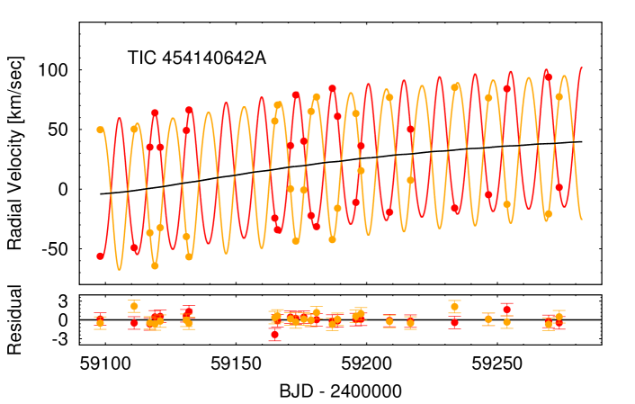
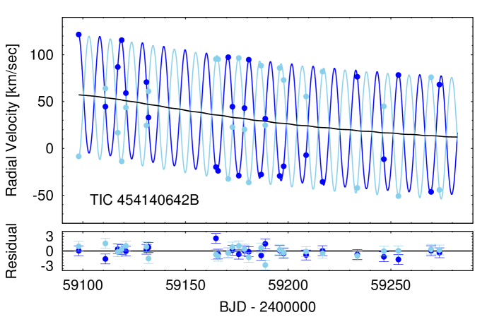
Figure 8: Radial velocities measured for TIC 454140642 (all individual RV values are given in Table LABEL:tbl:RVs). The solid curves represent the lowest $\chi^{2}$ spectro-photodynamical model solution (see in Sect. 5.1). The black curves show the RV contributions of the outer orbit. The residuals are also presented in the bottom panels. Note that the data obtained after JD 2 459 200 were not used for the analysis, although they agree perfectly with the solution.

Finally, we used the relative velocities and accelerations to derive a preliminary estimate of the outer orbital period and separation under the assumptions that the outer quadruple orbit (i) is being viewed nearly edge-on (i.e., $i_{\rm out}\simeq 90^{\circ}$), and (ii) can be approximated as circular. The former assumption is based on the fact that the EB orbits are both viewed nearly edge-on (but we caution that this is not a proof of the overall ‘flatness’ of the system). As for the assumption of a circular outer orbit, it is actually $e_{\rm out}\simeq 0.32$, but we proceeded under the circular orbit assumption to obtain a quick and simple estimate of the scope of the outer orbit. There are two equations that can be solved to find the outer orbital separation, $a_{\rm out}$, and phase, $\phi_{\rm out}$, at the time of the RV observations, where $\phi$ is the angle from inferior conjunction of binary A:

$$\sqrt{G(M_{A}+M_{B})/a}\,\sin\phi = \gamma_{A}-\gamma_{B}$$ (1)

$$G(M_{A}+M_{B})/a^{2}\cos\phi = \dot{\gamma}_{A}-\dot{\gamma}_{B}$$ (2)

If we solve for $a_{\rm out}$ and $\phi_{\rm out}$, and then calculate the outer period, $P_{\rm out}$ we find:

$$a_{\rm out}=389\pm 20~{}R_{\odot}$$

$$\phi=-38.8^{\circ}\pm 5^{\circ}$$

$$P_{\rm out}\simeq 419\pm 19~{}{\rm d}$$

where the uncertainties are due only to those associated with the measurements used in the calculations, and not to the actual eccentric nature of the outer orbit.

These approximations for the outer orbit served to guide the full photodynamical modeling described later.

Table 3: Radial Velocity Measurements for TIC 454140642^a

Observation Date	RV Aa	RV Ab	RV Ba	RV Bb
BJD $-$ 2,400,000	km s-1	km s-1	km s-1	km s-1
59097.9754	$-$56.29	+49.83	+121.71	$-$8.53
59110.9829	$-$49.11	+50.30	+44.69	+64.00
59117.0083	+35.20	$-$36.63	+86.98	+16.78
59118.9106	+63.97	$-$64.35	+115.66	$-$13.81
59120.9626	+35.06	$-$32.31	+59.15	+43.65
59130.9687	+49.18	$-$39.79	+70.83	+24.54
59131.9596	+66.35	$-$56.74	+33.01	+61.01
59164.8201	$-$24.29	+57.10	$-$19.90	+95.43
59165.8458	$-$34.06	+70.49	$-$23.97	+95.35
59170.8216	+36.46	+0.21	+97.46	$-$32.57
59172.8547	+78.94	$-$43.53	+44.59	+22.68
59175.9399	+40.22	$-$0.75	$-$29.14	+96.57
59178.7227	$-$22.22	+65.17	+43.06	+20.25
59180.7983	$-$31.47	+77.27	+94.78	$-$36.39
59186.8346	+84.48	$-$42.34	$-$27.90	+88.42
59188.8468	+61.05	$-$16.05	+31.70	+24.74
59195.8602	$-$11.14	+63.39	$-$29.43	+85.94
59197.8081	+36.24	+15.42	$-$19.08	+73.06
59199.7751	+82.82	$-$32.63	+47.12	+4.03
59208.7251	$-$19.33	+76.92	$-$7.22	+55.46
59216.7606	+50.26	+7.48	$-$35.74	+82.01
59233.6625	$-$15.88	+85.25	+76.54	$-$42.23
59246.6163	$-$4.70	+76.49	$-$11.52	+44.92
59253.6860	+84.15	$-$12.72	+78.43	$-$50.96
59269.6177	+93.88	$-$20.79	$-$46.47	+76.01
59273.6654	+1.48	+77.41	+68.18	$-$44.34

Notes. (a) RV measurements were taken with TRES on the 1.5 m reflector at the Fred Lawrence Whipple Observatory (FLWO) in Arizona. See text for details. The uncertainties on the individual measurements were determined empirically from the rms scatter in the residuals to the fitted model, and are 0.66, 0.73, 0.95, and 1.01 km s^-1 for stars Aa, Ab, Ba, and Bb, respectively.

Table 4: Preliminary Orbital Solutions for TIC 454140642

Fitted Binary Parametersa	Aa	Ab	Ba	Bb
Period [days]b	13.6239	13.6239	10.3928	10.3928
$K$ [km s-1]	$57.89\pm 0.41$	$60.79\pm 0.40$	$62.58\pm 0.51$	$65.05\pm 0.50$
$e$	$0.075\pm 0.005$	$0.075\pm 0.005$	$0.022\pm 0.004$	$0.022\pm 0.004$
$\omega$ [deg]	$354.9\pm 5$	$174.9\pm 5$	$1.9\pm 16$	$181.9\pm 16$
$\tau$c	$9159.9\pm 0.2$	$9159.9\pm 0.2$	$9149.9\pm 0.5$	$9149.9\pm 0.5$
$\gamma$ [km s-1]	$+11.34\pm 0.22$	$+11.34\pm 0.22$	$+41.17\pm 0.25$	$+41.17\pm 0.25$
$\dot{\gamma}$ [cm s-2]	$0.320\pm 0.006$	$0.320\pm 0.006$	$-0.331\pm 0.008$	$-0.331\pm 0.008$
Mass [$M_{\odot}$]d	$1.208\pm 0.018$	$1.151\pm 0.018$	$1.141\pm 0.019$	$1.098\pm 0.018$

Notes. (a) Derived from the RV measurements alone. (b) Fixed at the values given in Table 2. (c) BJD - 2450000. (d) Derived under the assumption that $\sin i\simeq 1$.

4.2 Photometric measurements

4.2.1 TESS Followup Observing Program

We acquired ground-based time-series follow-up photometry of TIC 454140642 as part of the TESS Follow-up Observing Program (TFOP). We used the TESS Transit Finder, which is a customized version of the Tapir software package (Jensen, 2013), to schedule our eclipse observations. The photometric data were extracted using AstroImageJ (Collins et al., 2017). Observations were acquired using the Las Cumbres Observatory network (LCO; Brown et al., 2013) and the Hazelwood Private Observatory (Churchill, Victoria, Australia) as described in Table 5.

Table 5: Summary of Ground-based Photometric Observations from TFOP

Telescope	Location	Date	Filter	Aperture radius	Coverage
		[UTC]		[arcsec]
TIC 454140642 Primary Eclipse
LCO-SAAO 0.4m	South Africa	2020-07-18	$z$-short	5.7	no event, ephemeris updated
LCO-McD 0.4m	Texas, U.S.	2020-09-08	$z$-short	6.8	no event, ephemeris updated
LCO-Hal 0.4m	Haleakala, U.S.	2020-10-20	$z$-short	4.0	ingress
LCO-SSO 0.4m	Siding Spring	2021-01-10	$z$-short	5.1	egress
Hazelwood 0.32m	Australia	2021-01-10	$i^{\prime}$	5.0	mid-eclipse
LCO-SAAO 0.4m	South Africa	2021-01-20	$z$-short	4.0	ingress
TIC 454140642 Secondary Eclipse
LCO-Hal 0.4m	Haleakala, U.S.	2020-09-18	$z$-short	8.6	no event, ephemeris updated
LCO-CTIO 0.4m	South Africa	2020-11-09	$z$-short	6.8	ingress

Notes. The $z$-short filter is the same as the Pan-STARRS Z-short pass-band, i.e. ${\rm\lambda_{center}=870~{}nm,~{}\lambda_{width}=104~{}nm}$. The $i^{\prime}$ filter is the same as the SDSS $i^{\prime}$ pass-band, i.e. ${\rm\lambda_{center}=755~{}nm,~{}\lambda_{width}=129~{}nm}$.

4.2.2 Other follow-up ground based photometry

In addition to the observations described above, we also used other photometric data for confirmation of the ETVs predicted from TESS data. These observations of eclipses of both pairs were obtained using the following instruments:

• FRAM telescopes: 30-cm telescope as part of the Pierre Auger Observatory in Argentina (The Pierre Auger Collaboration et al., 2021), and 25-cm telescope in La Palma as part of the Cherenkov Telescope Array (CTA) (Ebr et al., 2019).

• Ondřejov Observatory, Czech Republic, 65-cm reflecting telescope, using a G2-3200 CCD camera.

• Danish 1.54-m telescope located on La Silla in Chile, and using standard $V$ photometric filter.

• Small 34-mm refractor by R.U. - private observatory in Jílové u Prahy, Czech Republic, using a G2-0402 CCD camera.

4.2.3 Speckle Imaging

The target star was placed on the Southern Astrophysical Research Telescope (SOAR) speckle program in 2020 December. It was observed on 2021 February 27. The star was unresolved and no companions with $\rm\Delta I<1\ mag$ and having a separation greater than $\rm 0.048\arcsec$ were detected. The achieved detection limits are $\rm\Delta I<2.9\ mag$ at $\rm 0.15\arcsec$ and $\rm\Delta I<4.4\ mag$ at $\rm 1\arcsec$. The details of these observations will be published jointly with other SOAR speckle results as part of the series of papers represented by Tokovinin et al. (2020).

The A-B pair, with an estimated semimajor axis of 5 mas, is not expected to be resolved at SOAR. However, the speckle imaging demonstrated the absence of other nearby faint stars that could otherwise be missed by the photometry or spectroscopy. To the best of our knowledge, then, TIC 454140642 is an isolated quadruple system.

5 Analysis of System Parameters

Table 6: Times of minima of TIC 454140642 A

BJD	Cycle	std. dev.	BJD	Cycle	std. dev.	BJD	Cycle	std. dev.
$-2\,400\,000$	no.	$(d)$	$-2\,400\,000$	no.	$(d)$	$-2\,400\,000$	no.	$(d)$
54817.33051	-267.0	0.00100	56227.60857	-163.5	0.00016	59143.08895a	50.5	0.00027
54824.35102	-266.5	0.01293	56268.46600	-160.5	0.00019	59176.53298	53.0	0.00007
55130.58298	-244.0	0.00048	56574.59403	-138.0	0.00025	59183.95313	53.5	0.00007
55137.62361	-243.5	0.00069	58440.84110	-1.0	0.00028	59190.15168	54.0	0.00006
55171.45487	-241.0	0.00033	58448.26119	-0.5	0.00039	59197.57368	54.5	0.00006
55212.35313	-238.0	0.00043	58454.45985	0.0	0.00040	59244.61950a	58.0	0.00013
55859.75174	-190.5	0.00076	58461.88171	0.5	0.00045

Notes. Integer and half-integer cycle numbers refer to primary and secondary eclipses, respectively. Eclipses between cycle nos. $-267.0$ and $-138.0$ were observed in data from the WASP project. Times of minima from cycle no. $-1.0$ to $0.5$ and $53.0$ to $54.5$ are determined from the TESS measurements. Times of minima labeled with ^a are obtained from ground-based follow-up observations.

Table 7: Times of minima of TIC 454140642 B

BJD	Cycle	std. dev.	BJD	Cycle	std. dev.	BJD	Cycle	std. dev.
$-2\,400\,000$	no.	$(d)$	$-2\,400\,000$	no.	$(d)$	$-2\,400\,000$	no.	$(d)$
54766.52662	-354.0	0.00173	55873.51828	-247.5	0.00075	59162.70763a	69.0	0.00016
54813.46435	-349.5	0.00057	56268.45172	-209.5	0.00050	59178.45726	70.5	0.00038
54818.50060	-349.0	0.00025	56595.68135	-178.0	0.00023	59183.49229	71.0	0.00004
55109.43785	-321.0	0.00372	56647.61573	-173.0	0.00111	59188.84938	71.5	0.00033
55135.59379	-318.5	0.00024	56663.38911	-171.5	0.00024	59193.88343	72.0	0.00004
55156.38361	-316.5	0.00040	58440.54817	-0.5	0.00004	59199.24128	72.5	0.00026
55161.42771	-316.0	0.00077	58445.56571	0.0	0.00007	59214.66803a	74.0	0.00024
55208.38458	-311.5	0.00161	58455.95559	1.0	0.00006	59230.41337a	75.5	0.00033
55483.58635	-285.0	0.00042	58461.32839	1.5	0.00012	59235.45419a	76.0	0.00051

Notes. Integer and half-integer cycle numbers refer to primary and secondary eclipses, respectively. Eclipses between cycle nos. $-354.0$ and $-171.5$ were observed in the WASP project. Times of minima from cycle no. $-0.5$ to $1.5$ and $70.5$ to $72.5$ are determined from the TESS measurements. Times of minima labeled with ^a are obtained from ground-based follow-up observations.

5.1 Combined spectro-photodynamical analysis

We used the Lightcurvefactory software package (Borkovits et al., 2019, 2020a) to carry out a simultaneous, joint analysis of the lightcurves, ETV, RV curves and multi-passband SED data of the system. We used three separate lightcurves as follows:

• TESS Sectors 5 and 32 lightcurves. In the case of the Sector 32 data we used the 2-min cadence dataset for extracting the ETV data; however, for the joint analysis we binned these data into 1800 sec, resulting an effective exposure length of 1425-sec, to get the same sampling as was available for Sector 5 data. Furthermore, we excluded the flat out-of-eclipse lightcurve sections and kept only the narrow $\pm 0\@fp 03$-phase-domain regions around each eclipse.

• Similarly clipped regions of archival WASP data. After the removal of outlier data points, these data were averaged into 1800-sec bins for the analysis.

• The ground-based eclipse observations of our follow-up photometric campaign. These data were also binned at 1800 sec.

Additionally, we used the four ETV curves (primary and secondary ETV data for both binaries; see Tables 6 and 7), and the first 18 epochs of the four TRES RV curves (see Table LABEL:tbl:RVs). Furthermore, the observed passband magnitudes tabulated in Table 1 were also used for the SED analysis.

The modelling runs proceeded as follows. Lightcurvefactory calculates the positions and velocities of each star at any requested instant via the numerical integration of the orbital motion. Then, taking into account the radii, temperatures and other atmospheric properties of each star, and their relative geometry with respect to the others and to the observer, the code predicts the net lightcurve of the whole system, enabling any kind of mutual (or multiple) eclipses. Note that in the present analysis, stellar radii, and temperatures were constrained through the stellar masses and the metallicity and age of the system with the use of built-in PARSEC stellar isochrones (Bressan et al., 2012), as was described in Borkovits et al. (2020a) in detail. Furthermore, the same PARSEC tables are used for generating theoretical passband magnitudes for the SED fitting part of the analysis. To solve the inverse problem, Lightcurvefactory employs a Markov Chain Monte Carlo (MCMC)-based parameter search, implementing the generic Metropolis-Hastings algorithm (see e.g. Ford, 2005).

In most of the MCMC runs we adjusted the following 20 parameters:

• 4 orbital elements for binary A, i.e., the eccentricity and argument of periastron in the combinations of $(e\sin\omega)_{\mathrm{A}}$ and $(e\cos\omega)_{\mathrm{A}}$, its inclination, $i_{\mathrm{A}}$ and the longitude of the ascending node $\Omega_{\mathrm{A}}$ relative to the node of binary B;

• 3 orbital elements for binary B, i.e., the same as above with the exception of $\Omega_{\mathrm{B}}$, for which the value was kept at zero;

• 6 orbital parameters for the outer orbit, as its anomalistic period, $P_{\mathrm{AB}}$, eccentricity and argument of periastron, inclination, periastron passage time, $\tau_{\mathrm{AB}}$ and, the longitude of the ascending node relative to the node of binary B;

• 4 mass-related parameters, as the masses of the two primaries, $m_{\mathrm{Aa,Ba}}$), and the (inner) mass ratios of the two binaries, $q_{\mathrm{A,B}}$;

• 3 global parameters, as the (logarithmic) age of the system, its metallicity, [m/H], and the interstellar reddening $E(B-V)$.

Moreover, the following parameters were internally constrained:

• 4 remaining orbital parameters of the inner orbits, i.e., their periods ($P_{\mathrm{A,B}}$) and inferior conjunction times ($\mathcal{T}_{\mathrm{A,B}}^{\mathrm{inf}}$) at epoch $t_{0}$, which were constrained through the ETV curves (see Borkovits et al., 2019);

• The systemic radial velocity of the entire quadruple system ($\gamma$) was obtained at each step by minimizing the $\chi^{2}_{\mathrm{RV}}$ value a posteriori;

• 8 fundamental stellar parameters, i.e., the radii and temperatures of the four stars, which were interpolated from the PARSEC grids with the use of {mass, metallicity, age} triplets in the manner described by Borkovits et al. (2020a);

• The (photometric) distance of the system was also obtained through an a posteriori minimization of $\chi^{2}_{\mathrm{SED}}$;

• Finally, the (logarithmic) limb-darkening coefficients were calculated at each trial step internally from the pre-computed passband-dependent tables downloaded from the Phoebe 1.0 Legacy page. These tables were originally used in former versions of the Phoebe software (Prša & Zwitter, 2005).

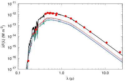
Figure 10: The summed SED of the four stars of TIC 454140642. The dereddened observed magnitudes are converted into the flux domain (red filled circles), and overplotted with the quasi-continuous summed SED for the quadruple star system (thick black line). This SED is computed from the Castelli & Kurucz (2003) ATLAS9 stellar atmospheres models (http://wwwuser.oats.inaf.it/castelli/grids/gridp00k2odfnew/fp00k2tab.html). The separate SEDs of the four stars are also shown with thin green, black and purple lines, respectively.

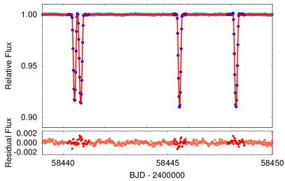
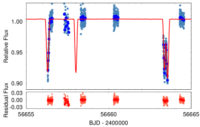
Figure 11: Photodynamical model (red line) plotted with the TESS data (left, blue) and WASP data (right, blue). Dark blue dots represent the data points used for fitting the photodynamical model. In the case of TESS data (left) these are the observed data points within the $\pm 0\@fp 03$ phase-domain of each eclipse, while in the case of the WASP observations (right) these are the 1800-sec averages of the individual data points. The pale blue points represent the remaining, out-of-eclipse TESS data (in the left panel), and the original WASP data (to the right). Residual curves are also plotted in the lower panels.

Table 8 lists the median values of the stellar and orbital parameters of the quadruple systems that are being either adjusted, internally constrained, or derived from the MCMC posteriors, together with their $1\sigma$ statistical uncertainties. The RV curves, lightcurves, ETV curves, and SED model of the lowest $\chi^{2}_{\mathrm{global}}$ solution are plotted in Figs. 8–11.

Table 8: Median values of the parameters from the double EB simultaneous lightcurve, $2\times$ SB2 radial velocity, double ETV, joint SED and PARSEC evolutionary track solution from Lightcurvefactory.

Orbital elementsa
	subsystem
	A		B		A–B
$P_{\mathrm{a}}$ [days]	$13.61594_{-0.00016}^{+0.00016}$		$10.39063_{-0.00008}^{+0.00008}$		$432.1_{-0.4}^{+0.5}$
semimajor axis [$R_{\odot}$]	$31.87_{-0.08}^{+0.12}$		$26.27_{-0.06}^{+0.07}$		$400.0_{-0.8}^{+1.0}$
$i$ [deg]	$87.55_{-0.06}^{+0.06}$		$87.52_{-0.08}^{+0.09}$		$87.69_{-0.47}^{+0.46}$
$e$	$0.07449_{-0.00021}^{+0.00021}$		$0.02700_{-0.00015}^{+0.00022}$		$0.32285_{-0.00497}^{+0.00501}$
$\omega$ [deg]	$161.21_{-0.56}^{+0.65}$		$190.89_{-1.19}^{+1.74}$		$325.77_{-1.18}^{+1.28}$
$\tau^{b}$ [BJD]	$2\,458\,437.0411_{-0.0204}^{+0.0240}$		$2\,458\,443.3691_{-0.0342}^{+0.0502}$		$2\,459\,070.05_{-1.25}^{+1.26}$
$\Omega$ [deg]	$-0.13_{-0.28}^{+0.29}$		$0.0$		$-0.15_{-0.26}^{+0.26}$
$(i_{\mathrm{m}})_{A-...}^{c}$ [deg]	$0.0$		$0.25_{-0.13}^{+0.20}$		$0.37_{-0.21}^{+0.34}$
$(i_{\mathrm{m}})_{B-...}$ [deg]	$0.25_{-0.13}^{+0.20}$		$0.0$		$0.47_{-0.24}^{+0.32}$
$\varpi_{\mathrm{dyn}}^{d}$ [deg ]	$11.04_{-1.35}^{+1.35}$		$161.21_{-0.55}^{+0.55}$		$325.82_{-1.19}^{+1.19}$
$i_{\mathrm{dyn}}^{d}$ [deg]	$0.31_{-0.17}^{+0.28}$		$0.41_{-0.21}^{+0.27}$		$0.06_{-0.04}^{+0.06}$
$i_{\mathrm{inv}}^{e}$ [deg]	$87.67_{-0.40}^{+0.38}$
$\Omega_{\mathrm{inv}}^{e}$ [deg]	$-0.13_{-0.24}^{+0.24}$
RV curve related parameters
mass ratio $[q=m_{\mathrm{sec}}/m_{\mathrm{pri}}]$	$0.959_{-0.006}^{+0.005}$		$0.964_{-0.005}^{+0.005}$		$0.963_{-0.013}^{+0.009}$
$K_{\mathrm{pri}}$ [km s-1]	$58.11_{-0.28}^{+0.24}$		$62.80_{-0.25}^{+0.24}$		$24.25_{-0.13}^{+0.13}$
$K_{\mathrm{sec}}$ [km s-1]	$60.62_{-0.20}^{+0.25}$		$65.14_{-0.21}^{+0.21}$		$25.20_{-0.16}^{+0.21}$
$\gamma$ [km/s]	$-$		$-$		$25.97_{-0.08}^{+0.07}$
Apsidal motion related parametersf
$U_{\mathrm{num}}$ [year]	$70$		$97$		$472$
$U_{\mathrm{theo}}$ [year]	$87_{-1}^{+1}$		$109_{-1}^{+1}$		$480_{-5}^{+5}$
$\Delta\omega_{\mathrm{3b}}$ [arcsec/cycle]	$556_{-5}^{+4}$		$338_{-3}^{+3}$		$3194_{-32}^{+31}$
$\Delta\omega_{\mathrm{GR}}$ [arcsec/cycle]	$0.611_{-0.003}^{+0.005}$		$0.709_{-0.003}^{+0.004}$		$0.106_{-0.001}^{+0.001}$
$\Delta\omega_{\mathrm{tide}}$ [arcsec/cycle]	$0.075_{-0.005}^{+0.004}$		$0.130_{-0.007}^{+0.009}$		$-$
Stellar parameters
	Aa	Ab	Ba	Bb
Relative quantities
fractional radius [$R/a$]	$0.0394_{-0.0006}^{+0.0005}$	$0.0365_{-0.0005}^{+0.0004}$	$0.0442_{-0.0005}^{+0.0007}$	$0.0415_{-0.0005}^{+0.0005}$
fractional flux [in TESS-band]	$0.305_{-0.008}^{+0.009}$	$0.246_{-0.008}^{+0.007}$	$0.247_{-0.009}^{+0.006}$	$0.204_{-0.008}^{+0.006}$
fractional flux [in SWASP-band]	$0.311_{-0.008}^{+0.010}$	$0.245_{-0.009}^{+0.008}$	$0.246_{-0.010}^{+0.007}$	$0.200_{-0.009}^{+0.007}$
fractional flux [in $R_{C}$-band]	$0.307_{-0.008}^{+0.009}$	$0.245_{-0.008}^{+0.007}$	$0.246_{-0.009}^{+0.007}$	$0.202_{-0.008}^{+0.007}$
Physical Quantities
$m$ [M⊙]	$1.195_{-0.009}^{+0.012}$	$1.146_{-0.012}^{+0.013}$	$1.146_{-0.007}^{+0.010}$	$1.105_{-0.008}^{+0.010}$
$R^{g}$ [R⊙]	$1.255_{-0.019}^{+0.018}$	$1.161_{-0.016}^{+0.018}$	$1.161_{-0.015}^{+0.019}$	$1.091_{-0.016}^{+0.015}$
$T_{\mathrm{eff}}^{g}$ [K]	$6434_{-29}^{+31}$	$6303_{-29}^{+31}$	$6303_{-29}^{+33}$	$6188_{-36}^{+34}$
$L_{\mathrm{bol}}^{g}$ [L⊙]	$2.420_{-0.090}^{+0.098}$	$1.917_{-0.081}^{+0.079}$	$1.917_{-0.082}^{+0.085}$	$1.570_{-0.077}^{+0.070}$
$M_{\mathrm{bol}}^{g}$	$3.81_{-0.04}^{+0.04}$	$4.06_{-0.04}^{+0.05}$	$4.06_{-0.05}^{+0.05}$	$4.28_{-0.05}^{+0.05}$
$M_{V}^{g}$	$3.81_{-0.04}^{+0.04}$	$4.07_{-0.05}^{+0.05}$	$4.07_{-0.05}^{+0.05}$	$4.29_{-0.05}^{+0.06}$
$\log g^{g}$ [dex]	$4.316_{-0.010}^{+0.013}$	$4.365_{-0.009}^{+0.011}$	$4.367_{-0.014}^{+0.010}$	$4.405_{-0.011}^{+0.010}$
Global Quantities
$\log$(age)g [dex]	$9.289_{-0.064}^{+0.045}$
$[M/H]^{g}$ [dex]	$-0.039_{-0.023}^{+0.022}$
$E(B-V)$ [mag]	$0.012_{-0.009}^{+0.013}$
$(M_{V})_{\mathrm{tot}}^{g}$	$2.54_{-0.03}^{+0.03}$
distance [pc]	$357_{-5}^{+4}$

Notes. (a) Instantaneous, osculating orbital elements at epoch $t_{0}=2\,458437.5$; (b) Time of periastron passsage; (c) Mutual (relative) inclination; (d) Longitude of pericenter ($\varpi_{\mathrm{dyn}}$) and inclination ($i_{\mathrm{dyn}}$) with respect to the dynamical (relative) reference frame (see text for details); (e) Inclination ($i_{\mathrm{inv}}$) and node ($\Omega_{\mathrm{inv}}$) of the invariable plane to the sky; (f) See Sect 6.3 for a detailed discussion of the tabulated apsidal motion parameters; (g) Interpolated from the PARSEC isochrones;

In addition to the usual orbital elements tabulated in the first section of Table 8, we list the mutual (i.e. relative to each other) inclinations of the three orbital planes as well (${i_{\mathrm{mut}}}_{A-B;A-AB;B-AB}$). We also provide the angular orbital elements in the dynamical frame of reference, i.e. the inclinations of the orbits relative to the invariable plane of the quadruple system ($i_{\mathrm{dyn}}$), and the longitude of the pericenter ($\varpi_{\mathrm{dyn}}=\Omega_{\mathrm{dyn}}+\omega_{\mathrm{dyn}}$) of each orbit defined as the sum of the dynamical longitude of the node and the dynamical argument of pericenter. We note that due to the almost perfect coplanarity of the entire system, the intersections of the three orbits with the invariable plane (and therefore all the three pairs of $\Omega_{\mathrm{dyn}}$ and $\omega_{\mathrm{dyn}}$) become ill-defined; however, their sums, i.e. $\varpi_{\mathrm{dyn}}=\Omega_{\mathrm{dyn}}+\omega_{\mathrm{dyn}}$ remain well-defined and we tabulate the latter quantities in Table 8. The relevance of these dynamical orbital elements lies in the fact that they, along with the mutual inclinations, appear directly in the analytic perturbation theories of multiple star systems (see, e.g. Borkovits et al., 2015, for further discussions). Furthermore, in this section we tabulate also some apsidal motion related parameters which will be discussed in Sect. 6.3. Finally, for completeness, we also provide the inclination and nodal angle of the invariable plane ($i_{\mathrm{inv}}$, $\Omega_{\mathrm{inv}}$, respectively).

We note that the values listed in Table 8 represent the (instantaneous) osculating orbital elements at the (arbitrarily chosen) epoch $t_{0}=2\,458437.5$. Therefore, the respective periods listed in the first row of the table should not be used for eclipse timing prediction for future follow-up observations. This is illustrated in Fig. 12 where we show the various relevant periods for the system. The osculating orbital elements (grey lines in the figure) are calculated at each instant from the Cartesian (Jacobian) coordinates and velocities of each orbit as if they represented pure, unperturbed, Keplerian two-body motions. In other words, these orbital elements describe the (osculating) two-body orbit on which the motion would continue if the perturbing forces vanished at that instant. The true motion occurs as the envelope of the osculating orbits. Naturally, in the presence of time-varying external forces such as those due to the gravitational perturbation from the second binary, the osculating elements vary continuously, with a characteristic period which is half of the orbital period of the given binary. Furthermore, if the outer orbit happens to be eccentric (as in the present case), the perturbing forces – as well as the amplitudes of the variations of the osculating elements – naturally increase around the periastron passage of the outer orbit. As a result, the value of a given osculating element depends strongly on the inner and outer orbital phase of the sampling. This is demonstrated in Fig. 12 by the green curve, which connects the anomalistic periods that were sampled during all the consecutive inner periastron passages of the given binary and, similarly, by the magenta curve which shows the osculating anomalistic periods during each primary eclipse. However, none of the periods discussed thus far can be observed. The periods that can be observed are, e.g. the time between two consecutive primary (or, secondary) eclipses or, in case of the RV observations, the repeating time of the RV curve. As both the eclipses and the RV curve are periodic according to the true longitude-like quantity $u=v+\omega$, where $v$ denotes the true anomaly and $\omega$ stands for the argument of periastron in the observational frame of reference, the measurable quantity is the $2\pi$ increment of $u$, instead of $v$, i.e. some kind of averaged sidereal (or, eclipsing) period, instead of an averaged anomalistic period. Therefore, in Fig. 12 we plot the time intervals between two consecutive primary (red) and secondary (blue) eclipses. One should be aware, however, that these observable eclipsing or, sidereal periods are systematically longer than the one-sidereal-period average of the instantaneous osculating anomalistic periods (brown symbols on the figure). The reason is that in a triple (and quadruple) system the clock of the inner binary is slowed as, on average, the perturbing forces from the outer bodies act as if the central mass of the binary were reduced. Finally, the black curve in Fig. 12 represents the average value of the eclipsing period which is practically the average of the red and blue curves, and can be determined most easily from the ETV curves as it is simply the linear term of the ETV ephemeris (as listed in the last row of Table 2, and in Fig. 9, as well).

5.2 PHOEBE analysis

For completeness, we also analyzed the TESS data via a classical light-curve modelling approach using the Wilson-Devinney method (Wilson & Devinney, 1971) as implemented in the PHOEBE code (Prša & Zwitter, 2005). Both binaries were analysed independently, using several simplifications for the analysis. Both orbital periods were kept fixed, and the mass ratio in each binary was set to the corresponding value given in Table 8. Likewise, the temperature of the primary in both binaries was taken from Table 8. See Table 9 for the results of the PHOEBE fit. These are in good agreement with those derived with the more sophisticated approach using the Lightcurvefactory code. Note, however, that the uncertainties associated with these PHOEBE results are statistical only, and have often been found to be underestimated.

Table 9: Calculated parameters from PHOEBE.

	Subsystem
	pair A		pair B
$i$ [deg]	$87.74\pm 0.08$		$87.40\pm 0.17$
$e$	$0.076\pm 0.003$		$0.027\pm 0.002$
$\omega$ [deg]	$158.1\pm 1.9$		$187.9\pm 5.4$
$q~{}[=m_{\mathrm{sec}}/m_{\mathrm{pri}}]$	$0.959~{}(\rm fixed)$		$0.964~{}(\rm fixed)$
Derived Physical Quantities
	Aa	Ab	Ba	Bb
relative flux $L_{TESS}$[%]	$29.7\pm 1.2$	$21.8\pm 2.0$	$28.3\pm 1.5$	$20.2\pm 1.8$
$T_{\mathrm{eff}}$ [K]	$6434~{}(\rm fixed)$	$6305\pm 26$	$6303~{}(\rm fixed)$	$6167\pm 30$
$R$ [R⊙]	$1.281\pm 0.008$	$1.106\pm 0.013$	$1.229\pm 0.012$	$1.061\pm 0.017$
$M_{\mathrm{bol}}$	$3.73\pm 0.05$	$4.14\pm 0.07$	$3.91\pm 0.06$	$4.32\pm 0.09$
$\log g$ [dex]	$4.300\pm 0.013$	$4.409\pm 0.015$	$4.317\pm 0.016$	$4.430\pm 0.017$

6 Discussion

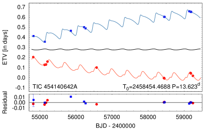
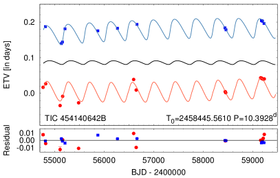
Figure 9: Eclipse timing variations of binaries A and B (left and right, respectively). Red circles and blue squares represent the observed primary and secondary eclipse times, respectively, while the corresponding solid lines represent the lowest $\chi^{2}$ spectro-photodynamical model solution. The black lines in the middle of both upper panels represent the pure Rømer delay (i.e., light-travel time) contribution to the given ETV. Residuals are also plotted in the lower panels.

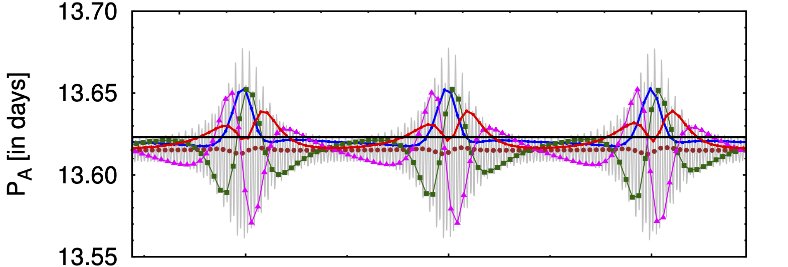
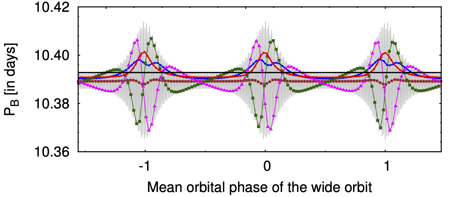
Figure 12: Illustration of the various periods discussed in the text for binaries A and B (upper and lower panels, respectively). The grey curves represent the (instantaneous), osculating anomalistic periods (as derived from the osculating true anomalies via Kepler’s third law). The brown circles represent the corresponding averages for one sidereal period of the binary (i.e., the interval during which the true longitude changes by $2\pi$). The dark-green squares represent the osculating anomalistic period at the time of each periastron passage of the corresponding binary, while magenta triangles denote the osculating anomalistic period at the time of the primary eclipses. The red/blue curves show the elapsed time between two primary/secondary eclipses, and can be considered to be the true, cycle-by-cycle sidereal (eclipsing) periods between two consecutive primary/secondary eclipses. Finally, the horizontal black lines represent the “average” sidereal (eclipsing) periods – i.e., the periods which can be obtained from the corresponding linear term in the long-term ETV fitting; these are the periods listed in Fig. 9.

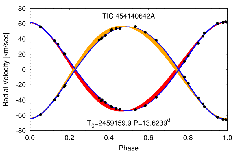
Figure 13: The folded RV curve of binary A, after the removal of the contribution of the outer orbit. Red and orange lines represent the fold of primary and secondary RV curves for the forthcoming 9.5 years. The consequence of the rapid, dynamically forced apsidal motion is clearly manifested in the varying shape of the curves. Black points represent the measured RVs (see in Table LABEL:tbl:RVs), while the blue lines represent the folded model curves during the interval of the observations. As one can see, the half-year duration of the available observations is insufficient to detect the apsidal motion, but it will be certainly detectable within a few years.

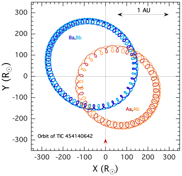
Figure 14: To-scale plot of the orbital motions in the quadruple TIC 454140642. The observer is in the $x-y$ plane and viewing the system from a distant position along the negative $y$ axis (i.e., the red arrow is the view direction).

6.1 Origin

This hierarchical system has several distinctive features pointing to its origin, namely (i) nearly equal masses of all four stars, (ii) a compact outer orbit, and (iii) a near-perfect coplanarity. It is well known that close binaries cannot form directly with their present-day small separations owing to the so-called ’opacity limit’ to fragmentation on the order of 10 au (e.g. Larson, 1972). Accretion of gas on to a nascent binary shrinks its orbit and at the same time increases the mass ratio because the secondary star accretes more; this mechanism can explain statistics of the close-binary population, including inner subsystems in hierarchies (Tokovinin & Moe, 2020). Preferential growth of the secondary component produces a subset of binaries with almost equal masses (twins) which is more prominent at short periods. A compact quadruple such as TIC 454140642 can be explained by the accretion-induced migration of both inner and outer subsystems, assuming that an initially wide and low-mass seed quadruple gained most of its mass by accretion. The seed quadruple could be produced, for example, through an encounter of two protostars A and B, each surrounded by a gas envelope. An encounter leads to a burst of accretion on to each star that produced the inner subsystems by disk fragmentation. However, other formation channels are also feasible. The important factor is a substantial mass growth of this progenitor quadruple by accretion that eventually created four stars with similar masses and shortened both inner and outer orbits. Dissipative interaction of the orbits with gas also led to the coplanarity of the entire system.

This formation scenario of compact 2+2 quadruples makes a strong prediction of near-equal masses and orbit alignment. Indeed, other known compact quadruples share these properties with TIC 45414062. The closest such system, VW LMi (11029+3025, HD 95660), has an outer period of 355 days and inner periods of 0.478 and 7.93 days (Pribulla et al., 2020). The masses of the stars in the closest eclipsing pair are not equal, but this could be a result of the later mass transfer; the other, 7.9-day subsystem is a twin with $q=0.98$, and the outer mass ratio is 0.93; all orbits are coplanar. Another compact and doubly-eclipsing quadruple V994 Her (= HD 170314) has an outer period of 2.9 yr and inner periods of 2.1 and 1.4 days (Zasche & Uhlař, 2016). The inner mass ratios are 0.86 and 0.95, and the outer mass ratio is 0.67. There is another, more distant star in this system. Finally, the doubly-eclipsing quadruple OGLE BLG-ECL-145467, found by Zasche et al. (2019), has an outer period of 4.2 yr, with inner periods of 3.3 and 4.9 days, and the masses of all four stars are comparable.

6.2 Gaia EDR3 Astrometry

The Gaia EDR3 astrometric excess noise for TIC 454140642 is 0.144 mas at a significance of $\sigma=24.476$; the number of good observations is 257 (Gaia EDR3, Gaia Collaboration 2020). The physical displacement corresponding to the excess noise is $\Delta a_{\rm measured}=0.052$ au (Eqn. 3, Belokurov et al. 2020). Taking into account the mass and luminosity ratios between binary A and B (0.94 and 0.8, respectively), as well as the eccentricity and argument of periastron of the AB system, the expected astrometric wobble is $\Delta a_{\rm expected}=0.053$ au (Eqn. 5, Belokurov et al. 2020) – practically identical to $\Delta a_{\rm measured}$. In addition, using the methodology of Stassun & Torres (2021) and the measured renormalized unit weight error (RUWE) of 1.299, the photocenter semi-major axis is 0.27 mas which, at the measured parallax of 2.786 mas, corresponds to $\approx 0.1$ au – comparable to $\Delta a_{\rm measured}$. Altogether, this indicates that Gaia has seen the astrometric wobble of the AB system.

6.3 Long-term Dynamical Stability and Orbital Evolution

The orbital elements listed in Table 8 represent a snapshot of the system at the reference epoch. Due to the strong dynamical interactions between the two binary stars, these orbital elements, in accordance with the perturbation theory of hierarchical stellar systems (see, e. g., Harrington, 1968) vary over time with at least three characteristic timescales: (i) the inner periods, (ii) the outer period and, (iii) the ratio of $P_{\mathrm{out}}^{2}/P_{\mathrm{in}}$ (see, e.g., Figs. 9, 12). The variations on the latter two timescales can nicely be confirmed on the ETV curves (Fig. 9), where, besides the strictly $P_{\mathrm{out}}$-period cyclic variations (not to be confused with the much smaller amplitude Rømer-delay, shown also in Fig. 9), the dynamically forced apsidal motion is also manifested.

To quantify the properties of the apsidal motions for all of the three orbits we calculated theoretical apsidal motion rates, $\Delta\omega$ (i.e. the variation of the argument of periastron, $\omega$, during one revolution of the given binary). For this approximate calculation, we used hierarchical three-body models. So, for example, to calculate the dynamical apsidal motion rate of binary A, we replaced the other binary (B) by a single outer body having mass $m_{\mathrm{B}}$ and, vice versa to compute the dynamical apsidal motion of binary B. Besides the dynamically forced apsidal motion, we also calculated the general relativistic and tidal contributions. For the two inner orbits we followed strictly the formulae and method described in Borkovits et al. (2015), Appendix C. For the outer orbit we considered the tidal contribution to be negligible and, furthermore, in the case of the dynamical term we simply calculated the algebraic sum of the contributions from the two separate ‘triple systems’ (formed by stars Aa,Ab,B and Ba,Bb,A). We list these apsidal advance rates in the ‘apsidal motion parameters’ part of Table 8.

As one can see, the dynamical apsidal advance rate ($\Delta\omega_{3b}$; where ‘3b’ stands for ‘third body’) is higher by 4-6 orders of magnitude than the relativistic and tidal rates ($\Delta\omega_{GR}$, $\Delta\omega_{\mathrm{tide}}$, respectively) for all the three orbits, therefore, these latter contributions are certainly negligible. Assuming that these apsidal motion rates remain nearly constant (which is a plausible assumption for such a nearly coplanar system) we estimated approximate theoretical apsidal motion periods for the three orbits. These periods were found to be $U_{\mathrm{theo}}=87\pm 1$, $109\pm 1$, and $480\pm 1$ years for binary A, B and AB, respectively.

In order to check the plausibility of our assumptions, we determined the ‘true’ apsidal motion periods of the three orbits. For this we numerically integrated the best-fit four-body model for $\sim 3\,000$ years, and then determined the average apsidal motion periods for all three orbits. We obtained $U_{\mathrm{num}}=70$, $97$, and $472$ years, respectively. Therefore, we can conclude that our simple, theoretical three-body model slightly overestimated the true periods (i.e., in other words, underestimated the amplitude of the perturbations a bit); however, it resulted in a correct estimation of their magnitude.

Finally we note that the rapid apsidal motion of binary A, in addition to the readily visible divergence of the primary and secondary ETV curves, will also be detectable within a few years through the variation of the shape of the RV curve of binary A. This is illustrated visually in Fig 13. (Note, despite the similarly rapid apsidal advance of binary B, due to its almost circular orbit, the same effect will remain below the uncertainties of the currently available RV data.)

We investigated also the short-term dynamical stability of the system. To confirm this we integrated the 4-body equations of motion for 5 million days (corresponding to $\approx 10,000$ outer periods), using the parameters from Table 8. We used the high-order IAS15 integrator with adaptive timesteps (Rein & Spiegel, 2015), part of the REBOUND N-body package (Rein & Liu, 2012). We provide a REBOUND jupyter notebook demonstrating the initialization and orbital element computation at https://github.com/vbkostov/TIC_454140642

As shown in Figure 16, there are no indications of chaotic motion and the system remains stable for the duration of said integration. The semi-major axis of binary A ($a_{A}$) oscillates between 31.8 $R_{\odot}$ and 32 $R_{\odot}$ and the eccentricity ($e_{A}$) varies between 0.066 and 0.082; the semi-major axis of binary B ($a_{B}$) oscillates between 26 $R_{\odot}$ and 26.2 $R_{\odot}$, and the eccentricity ($e_{B}$) varies between 0.023 and 0.030. The semi-major axis of binary AB ($a_{AB}$) oscillates between 400.6 $R_{\odot}$ and 402.5 $R_{\odot}$, and the eccentricity ($e_{AB}$) varies between 0.322 and 0.328. The orbital inclinations vary between $87.48^{\circ}$ and $87.85^{\circ}$ (binary A), $87.52^{\circ}$ and $87.81^{\circ}$ (binary B), and $87.64^{\circ}$ and $87.69^{\circ}$ (binary AB).

Figure 15: Upper panels: Evolution of the semimajor axis (left), eccentricity (middle), and inclination (right) of the two binaries and the quadruple over the course of 100,000 days (${\approx 230}$ outer periods). Lower panels: Same as above but zoomed-in to show the details around the 435-day outer orbit. We note that the periodic extrema in the semimajor axes and eccentricities correspond to the periastron passages of the outer orbit.

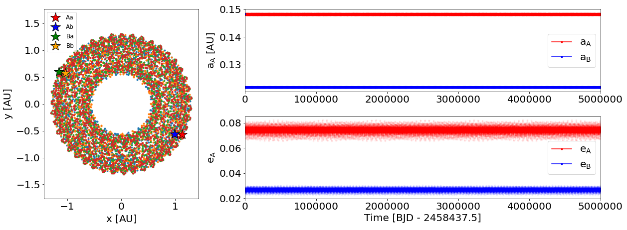
Figure 16: Left: The quadruple system as seen from above, highlighting the positions of all four stars (shown every 100 days) over the course of 200,000 days. The two binaries are separated by about an 1 au at closest approach. Upper right: Evolution of the semi-major axis of binary A and B (shown every 100 days) over the course of 5 million days (${\approx 10,000}$ outer periods), showing no indications of dynamical instability for the duration of the integration. Lower right: same as upper right but for the eccentricity of binary A and B.

Despite the near edge-on orientation of the system, there are no mutual eclipses or occultations between the constituents stars of binary A and binary B. This is highlighted in Figure 17 where we show the evolution of the respective impact parameters between the four stars. While there are periodic, precession-induced variations in the corresponding minimum impact parameters, the latter never reach below $\approx 4$.

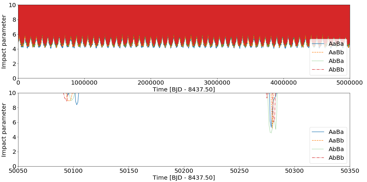
Figure 17: Upper panel: Evolution of the impact parameters between each star in each binary with respect to both stars of the other binary (e.g. AaBa for the impact parameter between Aa and Ba, AaBb for the impact parameter between Aa and Bb, etc.) over the course of 5 millions days days. Lower panel: same as above but zoomed-in on a 300-days interval to highlight two conjunctions.

7 Summary

We have presented the discovery of the quadruple-lined, doubly eclipsing quadruple system TIC 454140642. The target was observed by TESS in Sector 5 (at 30-min cadence) and again in Sector 32 (in 10-min cadence), and exhibited four sets of eclipses associated with two binary stars (A and B). Additional spectroscopic and photometric measurements reveal divergent radial velocities, eclipse-time variations and apsidal motion for both binaries, confirming that they form a gravitationally-bound quadruple system with a 2+2 hierarchy. The two binary stars have orbital periods of $P_{A}=13.62$ days and $P_{B}=10.39$ days, respectively, and slightly eccentric orbits ($e_{A}=0.07$, $e_{B}=0.03$). The four stars are very similar in terms of mass (individual masses between $1.105M_{\odot}$ and $1.195M_{\odot}$), size (radii between $1.09R_{\odot}$ and $1.26R_{\odot}$), and effective temperature (between 6188 K and 6434 K). The quadruple has an orbital period of $P_{AB}=432$ days and an eccentricity of $e_{AB}=0.32$. The entire system is essentially coplanar – the orbits of the two binaries and the wide orbit are aligned to within a fraction of a degree. TIC 454140642 is the newest addition to the small family of confirmed, well-characterized, multiply-eclipsing quadruple systems.

References

- Abadi et al. (2015) Abadi, M., Agarwal, A., Barham, P., et al. 2015, TensorFlow: Large-Scale Machine Learning on Heterogeneous Systems. https://www.tensorflow.org/
- Astropy Collaboration et al. (2013) Astropy Collaboration, Robitaille, T. P., Tollerud, E. J., et al. 2013, A&A, 558, A33, doi: 10.1051/0004-6361/201322068
- Astropy Collaboration et al. (2018) Astropy Collaboration, Price-Whelan, A. M., Sipőcz, B. M., et al. 2018, AJ, 156, 123, doi: 10.3847/1538-3881/aabc4f
- Bianchi et al. (2011) Bianchi, L., Herald, J., Efremova, B., et al. 2011, Ap&SS, 335, 161, doi: 10.1007/s10509-010-0581-x
- Borkovits et al. (2015) Borkovits, T., Rappaport, S., Hajdu, T., & Sztakovics, J. 2015, MNRAS, 448, 946, doi: 10.1093/mnras/stv015
- Borkovits et al. (2020a) Borkovits, T., Rappaport, S. A., Hajdu, T., et al. 2020a, MNRAS, 493, 5005, doi: 10.1093/mnras/staa495
- Borkovits et al. (2013) Borkovits, T., Derekas, A., Kiss, L. L., et al. 2013, MNRAS, 428, 1656, doi: 10.1093/mnras/sts146
- Borkovits et al. (2018) Borkovits, T., Albrecht, S., Rappaport, S., et al. 2018, MNRAS, 478, 5135, doi: 10.1093/mnras/sty1386
- Borkovits et al. (2019) Borkovits, T., Rappaport, S., Kaye, T., et al. 2019, MNRAS, 483, 1934, doi: 10.1093/mnras/sty3157
- Borkovits et al. (2020b) Borkovits, T., Rappaport, S. A., Tan, T. G., et al. 2020b, MNRAS, 496, 4624, doi: 10.1093/mnras/staa1817
- Borkovits et al. (2021) Borkovits, T., Rappaport, S. A., Maxted, P. F. L., et al. 2021, MNRAS, doi: 10.1093/mnras/stab621
- Brasseur et al. (2019) Brasseur, C. E., Phillip, C., Fleming, S. W., Mullally, S. E., & White, R. L. 2019, Astrocut: Tools for creating cutouts of TESS images. http://ascl.net/1905.007
- Bressan et al. (2012) Bressan, A., Marigo, P., Girardi, L., et al. 2012, MNRAS, 427, 127, doi: 10.1111/j.1365-2966.2012.21948.x
- Brown et al. (2013) Brown, T. M., Baliber, N., Bianco, F. B., et al. 2013, Publications of the Astronomical Society of the Pacific, 125, 1031, doi: 10.1086/673168
- Buchhave et al. (2010) Buchhave, L. A., Bakos, G. Á., Hartman, J. D., et al. 2010, ApJ, 720, 1118, doi: 10.1088/0004-637X/720/2/1118
- Burke et al. (2020) Burke, C. J., Levine, A., Fausnaugh, M., et al. 2020, TESS-Point: High precision TESS pointing tool, Astrophysics Source Code Library. http://ascl.net/2003.001
- Carter et al. (2011) Carter, J. A., Fabrycky, D. C., Ragozzine, D., et al. 2011, Science, 331, 562, doi: 10.1126/science.1201274
- Castelli & Kurucz (2003) Castelli, F., & Kurucz, R. L. 2003, in Modelling of Stellar Atmospheres, ed. N. Piskunov, W. W. Weiss, & D. F. Gray, Vol. 210, A20. https://arxiv.org/abs/astro-ph/0405087
- Chollet et al. (2015) Chollet, F., et al. 2015, Keras, https://keras.io
- Collins et al. (2017) Collins, K. A., Kielkopf, J. F., Stassun, K. G., & Hessman, F. V. 2017, AJ, 153, 77, doi: 10.3847/1538-3881/153/2/77
- Cutri et al. (2012) Cutri, R. M., Wright, E. L., Conrow, T., et al. 2012, Explanatory Supplement to the WISE All-Sky Data Release Products, Explanatory Supplement to the WISE All-Sky Data Release Products
- Dalcin et al. (2008) Dalcin, L., Paz, R., Storti, M., & D’Elia, J. 2008, Journal of Parallel and Distributed Computing, 68, 655, doi: http://dx.doi.org/10.1016/j.jpdc.2007.09.005
- De Rosa et al. (2014) De Rosa, R. J., Patience, J., Wilson, P. A., et al. 2014, MNRAS, 437, 1216, doi: 10.1093/mnras/stt1932
- Ebr et al. (2019) Ebr, J., Mandát, D., Pech, M., et al. 2019, arXiv e-prints, arXiv:1909.08085. https://arxiv.org/abs/1909.08085
- Feinstein et al. (2019) Feinstein, A. D., Montet, B. T., Foreman-Mackey, D., et al. 2019, PASP, 131, 094502, doi: 10.1088/1538-3873/ab291c
- Ford (2005) Ford, E. B. 2005, AJ, 129, 1706, doi: 10.1086/427962
- Fürész (2008) Fürész, G. 2008, PhD thesis, University of Szeged
- Gaia Collaboration et al. (2020) Gaia Collaboration, Brown, A. G. A., Vallenari, A., et al. 2020, arXiv e-prints, arXiv:2012.01533. https://arxiv.org/abs/2012.01533
- Harrington (1968) Harrington, R. S. 1968, AJ, 73, 190, doi: 10.1086/110614
- Harris et al. (2020) Harris, C. R., Millman, K. J., van der Walt, S. J., et al. 2020, Nature, 585, 357, doi: 10.1038/s41586-020-2649-2
- Henden et al. (2015) Henden, A. A., Levine, S., Terrell, D., & Welch, D. L. 2015, in American Astronomical Society Meeting Abstracts, Vol. 225, American Astronomical Society Meeting Abstracts #225, 336.16
- Høg et al. (2000) Høg, E., Fabricius, C., Makarov, V. V., et al. 2000, A&A, 355, L27
- Hunter (2007) Hunter, J. D. 2007, Computing in science & engineering, 9, 90
- Jensen (2013) Jensen, E. 2013, Tapir: A web interface for transit/eclipse observability, Astrophysics Source Code Library. http://ascl.net/1306.007
- Kochanek et al. (2017) Kochanek, C. S., Shappee, B. J., Stanek, K. Z., et al. 2017, PASP, 129, 104502, doi: 10.1088/1538-3873/aa80d9
- Kotikalapudi & contributors (2017) Kotikalapudi, R., & contributors. 2017, keras-vis, https://github.com/raghakot/keras-vis, GitHub
- Kovács et al. (2002) Kovács, G., Zucker, S., & Mazeh, T. 2002, A&A, 391, 369, doi: 10.1051/0004-6361:20020802
- Larson (1972) Larson, R. B. 1972, MNRAS, 156, 437, doi: 10.1093/mnras/156.4.437
- Latham et al. (2002) Latham, D. W., Stefanik, R. P., Torres, G., et al. 2002, The Astronomical Journal, 124, 1144, doi: 10.1086/341384
- Lightkurve Collaboration et al. (2018) Lightkurve Collaboration, Cardoso, J. V. d. M., Hedges, C., et al. 2018, Lightkurve: Kepler and TESS time series analysis in Python, Astrophysics Source Code Library. http://ascl.net/1812.013
- McKinney (2010) McKinney, W. 2010, in Proceedings of the 9th Python in Science Conference, ed. S. van der Walt & J. Millman, 51 – 56
- Moe & Di Stefano (2017) Moe, M., & Di Stefano, R. 2017, ApJS, 230, 15, doi: 10.3847/1538-4365/aa6fb6
- Nordstroem et al. (1994) Nordstroem, B., Latham, D. W., Morse, J. A., et al. 1994, A&A, 287, 338
- Pedregosa et al. (2011) Pedregosa, F., Varoquaux, G., Gramfort, A., et al. 2011, Journal of Machine Learning Research, 12, 2825
- Pérez & Granger (2007) Pérez, F., & Granger, B. E. 2007, Computing in Science and Engineering, 9, 21, doi: 10.1109/MCSE.2007.53
- Pollacco et al. (2006) Pollacco, D. L., Skillen, I., Collier Cameron, A., et al. 2006, PASP, 118, 1407, doi: 10.1086/508556
- Powell et al. (2021) Powell, B. P., Kostov, V. B., Rappaport, S. A., et al. 2021, AJ, 161, 162, doi: 10.3847/1538-3881/abddb5
- Pribulla et al. (2008) Pribulla, T., Baluďanský, D., Dubovský, P., et al. 2008, MNRAS, 390, 798, doi: 10.1111/j.1365-2966.2008.13781.x
- Pribulla et al. (2020) Pribulla, T., Puha, E., Borkovits, T., et al. 2020, MNRAS, 494, 178, doi: 10.1093/mnras/staa699
- Prsa et al. (2011) Prsa, A., Matijevic, G., Latkovic, O., Vilardell, F., & Wils, P. 2011, PHOEBE: PHysics Of Eclipsing BinariEs. http://ascl.net/1106.002
- Prša & Zwitter (2005) Prša, A., & Zwitter, T. 2005, ApJ, 628, 426, doi: 10.1086/430591
- Raghavan et al. (2010) Raghavan, D., McAlister, H. A., Henry, T. J., et al. 2010, ApJS, 190, 1, doi: 10.1088/0067-0049/190/1/1
- Rappaport et al. (2017) Rappaport, S., Vanderburg, A., Borkovits, T., et al. 2017, MNRAS, 467, 2160, doi: 10.1093/mnras/stx143
- Rein & Liu (2012) Rein, H., & Liu, S.-F. 2012, Astronomy & Astrophysics, 537, A128
- Rein & Spiegel (2015) Rein, H., & Spiegel, D. S. 2015, MNRAS, 446, 1424, doi: 10.1093/mnras/stu2164
- Rowden et al. (2020) Rowden, P., Borkovits, T., Jenkins, J. M., et al. 2020, AJ, 160, 76, doi: 10.3847/1538-3881/ab9d20
- Shappee et al. (2014) Shappee, B. J., Prieto, J. L., Grupe, D., et al. 2014, ApJ, 788, 48, doi: 10.1088/0004-637X/788/1/48
- Skrutskie et al. (2006) Skrutskie, M. F., Cutri, R. M., Stiening, R., et al. 2006, AJ, 131, 1163, doi: 10.1086/498708
- Stassun et al. (2018) Stassun, K. G., Oelkers, R. J., Pepper, J., et al. 2018, AJ, 156, 102, doi: 10.3847/1538-3881/aad050
- Szentgyorgyi & Furész (2007) Szentgyorgyi, A. H., & Furész, G. 2007, in Revista Mexicana de Astronomia y Astrofisica Conference Series, Vol. 28, Revista Mexicana de Astronomia y Astrofisica Conference Series, ed. S. Kurtz, 129–133
- The Pierre Auger Collaboration et al. (2021) The Pierre Auger Collaboration, Aab, A., Abreu, P., et al. 2021, accepted in Journal of Instrumentation, arXiv:2101.11602. https://arxiv.org/abs/2101.11602
- Tokovinin (2017) Tokovinin, A. 2017, MNRAS, 468, 3461, doi: 10.1093/mnras/stx707
- Tokovinin et al. (2020) Tokovinin, A., Mason, B. D., Mendez, R. A., Costa, E., & Horch, E. P. 2020, AJ, 160, 7, doi: 10.3847/1538-3881/ab91c1
- Tokovinin & Moe (2020) Tokovinin, A., & Moe, M. 2020, MNRAS, 491, 5158, doi: 10.1093/mnras/stz3299
- Toonen et al. (2016) Toonen, S., Hamers, A., & Portegies Zwart, S. 2016, Computational Astrophysics and Cosmology, 3, 6, doi: 10.1186/s40668-016-0019-0
- Torres et al. (2007) Torres, G., Latham, D. W., & Stefanik, R. P. 2007, ApJ, 662, 602, doi: 10.1086/516836
- Virtanen et al. (2020) Virtanen, P., Gommers, R., Oliphant, T. E., et al. 2020, Nature Methods, doi: https://doi.org/10.1038/s41592-019-0686-2
- Wilson & Devinney (1971) Wilson, R. E., & Devinney, E. J. 1971, ApJ, 166, 605, doi: 10.1086/150986
- Zasche & Uhlař (2016) Zasche, P., & Uhlař, R. 2016, A&A, 588, A121, doi: 10.1051/0004-6361/201628153
- Zasche et al. (2019) Zasche, P., Vokrouhlický, D., Wolf, M., et al. 2019, A&A, 630, A128, doi: 10.1051/0004-6361/201936328
- Zasche et al. (2020) Zasche, P., Henzl, Z., Lehmann, H., et al. 2020, A&A, 642, A63, doi: 10.1051/0004-6361/202038656