On Secrecy Performance of Mixed $\alpha-\eta-\mu$ and Málaga RF-FSO Variable Gain Relaying Channel

Abstract

With the completion of standardization of fifth-generation (5G) networks, the researchers have begun visioning sixth-generation (6G) networks that are predicted to be human-centric. Hence, similar to 5G networks, besides high data rate, providing secrecy and privacy will be the center of attention by the wireless research community. To support the visions beyond 5G (B5G) and 6G, in this paper we propose a secure radio frequency (RF)-free space optical (FSO) mixed framework under the attempt of wiretapping by an eavesdropper at the RF hop. We assume the RF links undergo $\alpha-\eta-\mu$ fading whereas the FSO link exhibits a unified Málaga turbulence model with pointing error. The secrecy performance is evaluated by deducing expressions for three secrecy metrics i.e. average secrecy capacity, secure outage probability, and probability of non-zero secrecy capacity in terms of univariate and bivariate Meijer’s $G$ and Fox’s $H$ functions. We further capitalize on these expressions to demonstrate the impacts of fading, atmospheric turbulence, and pointing errors and show a comparison between two detection techniques (i.e. heterodyne detection (HD) and intensity modulation with direct detection (IM/DD)) that clearly reveals better secrecy can be achieved with HD technique relative to the IM/DD method. The inclusion of generalized fading models at the RF and FSO hops offers unification of several classical scenarios as special cases thereby exhibiting a more generic nature relative to the existing literature. Finally, all the analytical results are corroborated via Monte-Carlo simulations.

Keywords: $\alpha-\eta-\mu$ fading, Málaga turbulence, pointing error, physical layer security, secure outage probability,Variable Gain Relaying, RF/FSO Communication.

1 Introduction

1.1 Background

The ever increasing demand for higher data rates at lower costs has been the motivation for researchers to explore new data transfer technologies. As a result, the data transfer speed is increasing with every generation of the communication systems. In this era of fifth-generation (5G) communications and beyond (B5G), technicians are targeting to achieve a data rate of 1 Gbps [1]. To achieve this very high-speed data transfer, free-space optical (FSO) technologies can be a great medium of data communication.

As 5G is already deployed in many areas of the world, researchers have already begun their work on 6G communications where the security of information and privacy of the users is going to be prioritized. The authors in [2] suggested that as the encryption method is failing to provide the necessary security against the powerful computing systems, physical layer security (PLS) can be a better option for ensuring secrecy. They also suggested that visible light communications (in other words FSO communications) can be put to use to achieve this goal. The application of FSO via UAVs can also be a great solution to the bandwidth requirements and security problem that arises in 6G communications [3]. At present, the FSO network is being applied to military communications, metropolitan area network (MAN) extensions, and to resolve the “last mile access” problem [4]. Although the FSO networking system has numerous advantages, it is yet to be considered for deployment at a large scale because of its short-range transmission capacity. This disadvantage can be easily removed by the hybridization of radio frequency (RF) and FSO networks that will provide us all the advantages provided by both RF and FSO systems. Such hybrid RF-FSO communication systems can transmit data at long distances with high data rates [5].

1.2 Literature Survey

The advantages presented by RF-FSO networks has caught the attention of researchers that has led them to analyze the possibility of real-life applications of such hybrid systems. The performance of RF-FSO networks for the simplest of combinations of communication nodes (assuming only a single source, an amplify-and-forward (AF) relay, and a receiver) was analyzed in [6, 7, 8, 9] considering the effects of turbulence and pointing errors at the FSO link. A similar model was also analyzed in [10, 11] but in these works, the authors considered decode-and-forward (DF) relaying scheme instead of the AF relay. A cognitive radio network was also employed with an underlay RF-FSO system in [12, 13, 14, 15] as it is a viable solution that can be used in metropolitan networking. The authors in [16] designed a RF-FSO cloud computing-based radio access network (CC-RAN) for 5G communication with Rayleigh and Gamma-Gamma (GG) fading models at the RF and FSO hop, respectively, considering multiple senders. As generalized fading models allow us the versatility of using multiple multipath fading models without any complex mathematical manipulation, researchers started employing them in RF-FSO networks for enhancing its performance. Due to this reason, another CC-RAN was evaluated with $\kappa-\mu$ shadowed fading and exponentiated Weibull (EW) fading models at the RF and FSO hops, respectively, considering a single [17] and multiple users [18].

Researchers have also considered some more complex communication scenarios within RF-FSO communication technologies to reduce the disadvantages caused by pointing error or turbulence at FSO hop. Authors in [19, 20, 21] evaluated a scenario where multiple sources are sending data to the relay and the relay is multiplexing and retransmitting that information to the receiver through the FSO link. An analogous model was considered in [22] where the information from multiple sources is re-transmitted via a relay to the receiver using time division multiple access (TDMA) techniques. The advantages of transmit antenna selection (TAS) scheme was perused in [23] over a RF-FSO system considering multiple receivers. A data transfer scenario with both direct and relay assisted links was explored in [24, 25] where the relay assisted link was a RF-FSO link with both sender and receiver having multiple antennas and multiple receiver apertures, respectively [24]. The capacity of a FSO link can be enhanced by employing a multiple-input multiple-output (MIMO) configuration that was shown in [26, 27]. In [28], authors described a very unique scenario in a RF-FSO network where both the relay and the destination had RF antennas and optical apertures so the relay was able to send information using RF or optical signals and the receiver could receive both the signals. A comparison was then made between single-input single-output (SISO) and dual-input dual-output (DIDO) based relay systems applied to a RF-FSO configuration where the authors concluded that DIDO outperforms SISO significantly [29]. The relay selection scheme was employed in [30] to enhance the performance of a system having multiple sources. A few works also show a reverse technology where the authors have considered FSO technology as the source to relay link and RF technology for relay to destination link [31, 32, 33, 34] where the authors in [32, 33, 34] have considered multiple receivers at the RF hop.

In the present era, ensuring high data speed is not enough if the transmission of information is insecure. In the early stages of wireless communications, the cryptographic approach was more popular among the researchers. But due to the requirement of high power and complexity, this method is losing its popularity [35]. On the other hand, PLS has emerged as an auspicious paradigm for information security against malicious attackers. Researchers around the world have started analyzing the PLS for RF-FSO communication technology. A general eavesdropping scenario for RF-FSO systems was assumed in [36, 37, 38, 39] where the eavesdropper is trying to overhear the legitimate information through the RF link. Similar RF-FSO models have also been subjected to the secrecy analysis considering transmit antenna selection (TAS) schemes [40] and maximal ratio combining (MRC) technique at both relay and eavesdropper [41]. An opportunistic user scheduling (OUS) mechanism in RF-FSO network with multi-antenna relay and eavesdropper was interpreted in [42]. Authors in [43] made a trade-off between security and reliability for an OUS relay network with power allocation. Security of the system can be hampered if multiple eavesdroppers are present in the system that was shown in [44]. Researchers have found that this problem can be solved by using the partial relay selection scheme [45].

1.3 Motivation and Contributions

In physical layer communication over both RF and FSO links, a variation takes place to the transmitted signal due to the random physical properties of the channels through which the information is transmitted. Since this randomness of the wireless channels can not be predicted beforehand, and the channels between the transmit and receive nodes are changing at each and every instant, hence assuming a generalized scenario at these links has proven to be more practical. This is why the researchers around the world started considering generalized channels for evaluating the performance of wireless communication systems. In a mixed RF-FSO system, although some generalized RF channels, e.g. $\eta-\mu$, hyper Gamma, and generalized Gamma [37, 38, 39, 46, 47, 48], etc. have been considered, these channels do not cover all the physical aspects of communication through a wireless medium. To remedy this situation, the generalized $\alpha-\eta-\mu$ channel is considered in this work as the RF link that incorporates the non-homogeneity and the non-linearity nature of the fading channels with no line-of-sight (LOS) component [49]. Furthermore, the $\alpha-\eta-\mu$ fading distribution includes $\alpha-\mu$ and $\eta-\mu$ generalized fading scenarios along with their special multipath cases such as Nakagami-$m$, Nakagami-$q$, Rayleigh, and Weibull [50]. On the other hand, the FSO link of this work is considered to follow the well-known unified Málaga model with pointing error impairments that also represents a generalized scenario by including GG, Log-Normal, Rice-Nakagami, etc. distributions as its special cases [51, 52]. As a result, the proposed ($\alpha-\eta-\mu$)-Málaga RF-FSO mixed distribution can cover a wide variety of mixed configurations that can handle any practical scenario more precisely relative to the existing literature.

• First of all, we derive the expressions of dual-hop cumulative distribution functions (CDFs) for the proposed RF-FSO system utilizing the probability density functions (PDFs) of $\alpha-\eta-\mu$ and Málaga fading distributions considering variable gain relaying technique. The derived CDFs are completely unique and can be utilized to derive the dual-hop CDFs of [37] and [39] as our special cases.

• We analyze the secrecy performance of the proposed system incorporating the impact of atmospheric turbulence, fading parameters, and pointing error. The expressions of average secrecy capacity (ASC), lower bound of secrecy outage probability (SOP), and probability of non-zero secrecy capacity (PNSC) are derived in terms of well-known univariate and bivariate Meijer’s $G$ and Fox’s $H$ functions. The derived expressions are novel and can be utilized to replicate the results of [36, 37]. A comparative study is also presented between HD and IM/DD techniques for better clarification.

• Monte-Carlo (MC) simulations are provided for verifying the accuracy of the derived analytical expressions of ASC, lower bound of SOP, and PNSC.

• Our analysis suggests the system security boosts up with the reduction of severity of atmospheric turbulence, enhancement of the values of fading parameters, and increment in the value of pointing error. Moreover, the PLS of the considered model always exhibits superior performance under the HD technique relative to the IM/DD technique.

1.4 Organization

The rest of this paper is organized in the following manner. Section II narrates the proposed system model along with mathematical formulation. Section III derives the closed-form expressions for performance parameters (ASC, lower bound of SOP, and PNSC). Section IV demonstrates numerical results for these derived performance parameters via utilizing graphical representations followed by summarizing the work in Section VI.

2 System Model and Problem Formulation

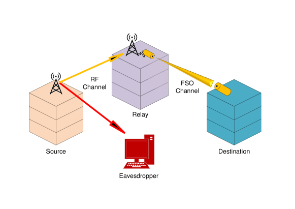
Figure 1: Dual hop RF-FSO system including a source ($A_{s}$), a relay ($B_{r}$), a destination ($C_{d}$), and an eavesdropper ($E_{v}$).

Our proposed system model is demonstrated in Fig. 1, which includes a source ($A_{s}$), a relay ($B_{r}$), a destination ($C_{d}$), and an eavesdropper ($E_{v}$). Each of $A_{s}$ and $E_{v}$ are equipped with a single antenna whereas $B_{r}$ and $C_{d}$ have a single aperture for transmission and reception of optical signals, respectively. We consider the destination receives transmitted RF signal from source in optical form whereby the RF to optical conversion is performed at the relay node. On the other hand, eavesdropper takes advantage of the time varying nature of RF link while it is on a continuous hunt to steal information via source to eavesdropper ($A_{s}-E_{v}$) link. The source to relay ($A_{s}-B_{r}$) and $A_{s}-E_{v}$ links are assumed to follow independently distributed $\alpha-\eta-\mu$ fading whereas the relay to destination ($B_{r}-C_{d}$) link experiences Málaga turbulence impaired with pointing error. The motivation behind selecting these two distributions is that both $\alpha-\eta-\mu$ and Málaga turbulence fading models provide excellent match with the experimental data [53, 54]. Moreover, the $\alpha-\eta-\mu$ fading model has the highest accuracy to represent the variation in transmitted signals over various different multipath fading channels [53].

2.1 RF Channel Model

Denoting the channel gain of $A_{s}-B_{r}$ link as $a_{sr}$ and the corresponding SNR as $\gamma_{r}=\frac{P_{s}}{N_{r}}\|a_{sr}^{2}\|$, where $P_{s}$ and $N_{r}$ are the transmit power of $A_{s}$ and noise power at $B_{r}$, respectively. We can express the PDF of $\gamma_{r}$ as [49]

$$f_{r}(\gamma) =\frac{S_{r}}{{\omega}_{r}^{\beta_{r}}}\gamma^{\beta_{r}-1}e^{-A_{r}(\frac{\gamma}{{\omega}_{r}})^{\tilde{\alpha}_{r}}}I_{\mu_{r}-\frac{1}{2}}\biggl{(}P_{r}\left(\frac{\gamma}{{\omega}_{r}}\right)^{\tilde{\alpha_{r}}}\biggl{)},$$ (1)

where $S_{r}=\frac{\sqrt{\pi}{\tilde{\alpha}_{r}}\mu_{r}^{\mu_{r}+\frac{1}{2}}(\eta_{r}-1)^{\frac{1}{2}-\mu_{r}}(\eta_{r}+1)^{\mu_{r}+\frac{1}{2}}}{\eta_{r}\Gamma(\mu_{r})}$, $A_{r}=\frac{\mu_{r}(1+\eta_{r})^{2}}{2\eta_{r}}$, $\beta_{r}={\tilde{\alpha}_{r}}({\mu_{r}+\frac{1}{2})}$, $P_{r}=\frac{\mu_{r}({\eta_{r}}^{2}-1)}{2\eta_{r}}$, and $\tilde{\alpha}_{r}=\frac{\alpha_{r}}{2}$. Here, the average SNR is denoted by ${\omega}_{r}$, $I_{r}(.)$ represents the first-order modified Bessel function as defined in [55, Eq. (9.6.20),], non-linearity parameter is denoted by ${\alpha}_{r}$, the number of multipath clusters is denoted by $\mu_{r}$, and the ratio between in-phase and quadrature scattered wave components is denoted by $\eta_{r}$. Making use of [56, Eq. (8.445),] and employing mathematical simplifications and manipulations, we can write $f_{r}(\gamma)$ as

$$f_{r}(\gamma)=\sum_{N_{1}=0}^{\infty}u_{1}\gamma^{u_{3}}e^{{-u_{2}}{\gamma^{\tilde{\alpha}_{r}}}},$$ (2)

where $u_{1}$=$\frac{S_{r}\left(\frac{P_{r}}{{2\omega}_{r}^{{\tilde{\alpha}_{r}}}}\right)^{{\mu_{r}-\frac{1}{2}}+2N_{1}}}{N_{1}!{\omega}_{r}^{\beta_{r}}\Gamma({\mu_{r}+\frac{1}{2}}+N_{1})}$, $u_{2}$=$(\frac{A_{r}}{{\omega}_{r}^{\tilde{\alpha}_{r}}})$, and $u_{3}$=${\tilde{\alpha}_{r}}({\mu_{r}-\frac{1}{2}}+2N_{1})+\beta_{r}-1$. We define the CDF of $\gamma_{r}$ as

$$F_{r}(\gamma)=\int_{0}^{\gamma_{r}}f_{r}(\gamma)d\gamma.$$ (3)

Placing (2) into (3) and utilizing [56, Eqs. (3.381.8) and (8.352.6,], we obtain the final expression for CDF of $\gamma_{r}$ as

$$F_{r}(\gamma)=1-\sum_{N_{1}=0}^{\infty}\sum_{t_{1}=0}^{W_{1}-1}u_{4}{e^{-u_{2}\gamma^{\tilde{\alpha}_{r}}}\gamma^{\tilde{\alpha}_{r}t_{1}}},$$ (4)

where $W_{1}=\frac{u_{3}+1}{\tilde{\alpha}_{r}}$ and $u_{4}=(W_{1}-1)!\frac{u_{1}}{\tilde{\alpha}_{r}{u_{2}}^{W_{1}}}\frac{{u_{2}}^{t_{1}}}{t_{1}!}$.

2.2 FSO Channel Model

Denoting the channel gain of $B_{r}-C_{d}$ link as $a_{rd}$, we can define the corresponding SNR as $\gamma_{d}=\frac{P_{r}}{N_{d}}\|a_{rd}^{2}\|$, where $P_{r}$ and $N_{d}$ symbolize the transmit power from relay and noise power at the destination, respectively. We assume $\gamma_{d}$ follows the unified Málaga distribution with pointing error, the PDF of which can be expressed as [57]

$$f_{d}(\gamma)=\frac{{\varepsilon}^{2}A_{d}}{2^{r}\gamma}\sum_{\tilde{m}_{d}=1}^{{\beta}_{d}}b_{d}G_{1,3}^{3,0}\left[B_{d}\left(\frac{\gamma}{u_{r}}\right)^{\frac{1}{r}}\biggl{|}\begin{array}[]{c}{\varepsilon}^{2}+1\\ {\varepsilon}^{2},{{\alpha}_{d}},{\tilde{m}_{d}}\\ \end{array}\right],$$ (7)

where

$$A_{d}=\frac{2{\alpha_{d}}^{\frac{\alpha_{d}}{2}}}{g_{d}^{1+\frac{\alpha_{d}}{2}}\Gamma(\alpha_{d})}\biggl{(}\frac{g_{d}\beta_{d}}{g_{d}\beta_{d}+\Omega_{d}}\biggl{)}^{\beta_{d}+\frac{\alpha_{d}}{2}},$$

$$B_{d}=\frac{\varepsilon^{2}\alpha_{d}\beta_{d}(g_{d}+\Omega_{d})}{(\varepsilon^{2}+1)(g_{d}\beta_{d}+\Omega_{d})},$$

$$a_{d}=\binom{\beta_{d}-1}{\tilde{m}_{d}-1}\frac{(g_{d}\beta_{d}+\Omega_{d})^{1-\frac{\tilde{m}_{d}}{2}}}{(\tilde{m}_{d}-1)!}{\biggl{(}\frac{\Omega_{d}}{g_{d}}\biggl{)}^{\tilde{m}_{d}-1}}\biggl{(}\frac{\alpha_{d}}{\beta_{d}}\biggl{)}^{\frac{\tilde{m}_{d}}{2}},\text{ and}$$

$$b_{d}=\alpha_{d}\biggl{(}\frac{\alpha_{d}\beta_{d}}{g_{d}\beta_{d}+\Omega_{d}}\biggl{)}^{-\frac{\alpha_{d}+\tilde{m}_{d}}{2}}.$$

In (7), the electrical SNR is denoted by $u_{r}$, where the optical signal detection system is referred by $r$ i.e. $r=1$ is meant for HD technique with $u_{HD}=\bar{\gamma}_{d}$ and $r=2$ is meant for IM/DD technique with $u_{IM/DD}=\frac{\alpha_{d}{\varepsilon}^{2}(g_{d}+\Omega_{d})({\varepsilon}^{2}+2)}{(\varepsilon^{2}+1)^{2}(\alpha_{d}+1)[2g_{d}(g_{d}+2\Omega_{d})+{\Omega_{d}}^{2}(1+\frac{1}{\beta_{d}})]}\bar{\gamma}_{d}$ [57], and $\overline{\gamma}_{d}$ is the average SNR. The effective number of large scale cells during scattering process is denoted by $\alpha_{d}$, natural number $\beta_{d}$ represents fading parameter’s amount, the average power of the scattering component in the off-axis eddies is denoted by $g_{d}=\mathbb{E}[{|U_{s}^{g}|}^{2}]=2b_{d}(1-\rho)$, $2b_{d}=\mathbb{E}[{{|U_{s}^{c}|}^{2}}+{{|U_{s}^{g}|}^{2}}]$ denotes the average power of scattering components, the average power from the coherent contributions is represented by $\Omega_{d}$, where $\Omega_{d}=\Omega+2b_{d}\rho+2\sqrt{2b_{d}\rho\Omega}\cos(\Theta_{A}-\Theta_{B})$ refers to the average power regarding coherent advantages, regular power through LOS component is defined by $\Omega=\mathbb{E}[{|U_{los}|}^{2}]$, the deterministic phases of LOS and coupled-to-LOS spread terms are referred by $\Theta_{A}$ and $\Theta_{B}$, respectively. Here, the amount of coupling between scattering components and LOS component is described with a range of $0\leq\rho\leq 1$, the quantity of scattering power coupled LOS component is denoted by $0\leq\rho\leq 1$ [57], and the ratio of the equivalent beam radius to the pointing error displacement standard deviation (jitter) at the receiver is referred by $\varepsilon$. The Meijer’s $G$ function is symbolized by $G[.]$ that is defined in [56]. The CDF of $\gamma_{d}$ is given by [57, Eq. (9),]

$$F_{d}(\gamma)=\sigma\sum_{\tilde{m}_{d}=1}^{\beta_{d}}c_{d}G_{r+1,3r+1}^{3r,1}\left[\frac{F}{u_{r}}\gamma\biggl{|}\begin{array}[]{c}1,l_{1}\\ l_{2},0\\ \end{array}\right],$$ (10)

where $\sigma$=$\frac{\varepsilon^{2}A_{d}}{2^{r}(2\pi)^{r-1}}$, $F$=$\frac{{B_{d}}^{r}}{r^{2r}}$, $c_{d}$=${b_{d}}r^{\alpha_{d}+\tilde{m_{d}}-1}$, $l_{1}=[\Delta(r,\varepsilon^{2}+1)]$ that includes $r$ terms, and $l_{2}=[\Delta(r,\varepsilon^{2}),\Delta(r,\alpha_{d}),$ $\Delta(r,\tilde{m}_{d})]$ that includes $3r$ terms. Here, $\Delta$ defines the series such as $\Delta(a,b)=(\frac{b}{a},\frac{b+1}{a},......,\frac{b+a-1}{a})$.

2.3 RF-FSO Mixed Channel Model

Considering variable gain AF relaying scheme, the equivalent SNR at the destination terminal for the dual-hop RF-FSO mixed system is denoted as $\gamma_{o}=\frac{\gamma_{r}\gamma_{d}}{\gamma_{r}+\gamma_{d}+1}\approx\min(\gamma_{r},\gamma_{d})$ [36, Eq. 7,] and the corresponding CDF is given by [58, Eq. 10,]

$$F_{d}(\gamma) =\Pr\left\{\min\left\{\gamma_{r},\gamma_{d}\right\}<\gamma\right\}$$

$$=F_{r}(\gamma)+F_{d}(\gamma)-F_{r}(\gamma)F_{d}(\gamma).$$ (11)

By substituting (2) and (3) into (2.3), we obtain

$$F_{o}(\gamma) =1-\sum_{N_{1}=0}^{\infty}\sum_{t_{1}=0}^{W_{1}-1}u_{4}{e^{-u_{2}\gamma^{\tilde{\alpha}_{r}}}\gamma^{\tilde{\alpha}_{r}t_{1}}}\left(1-\sigma\sum_{\tilde{m}_{d}=1}^{\beta_{d}}c_{d}G_{r+1,3r+1}^{3r,1}\left[\frac{F}{u_{r}}\gamma\biggl{|}\begin{array}[]{c}1,l_{1}\\ l_{2},0\\ \end{array}\right]\right).$$ (14)

2.4 RF Channel Model

We consider the eavesdropper channel also undergoes $\alpha-\eta-\mu$ fading. Hence, denoting the channel gain of $A_{s}-E_{v}$ link as $a_{sv}$ and corresponding SNR as $\gamma_{v}=\frac{P_{s}}{N_{v}}\|a_{sv}^{2}\|$, where $N_{v}$ is the noise power at $E_{v}$, we can express the PDF of $\gamma_{v}$ as [49]

$$f_{v}(\gamma) =\frac{S_{v}}{{\omega}_{v}^{\beta_{v}}}\gamma^{\beta_{v}-1}e^{-A_{v}(\frac{\gamma}{{\omega}_{v}})^{\tilde{\alpha}_{v}}}I_{\mu_{v}-\frac{1}{2}}\biggl{(}P_{v}(\frac{\gamma}{{\omega}_{v}})^{\tilde{\alpha_{v}}}\biggl{)},$$ (15)

where $S_{v}=\frac{\sqrt{\pi}{\tilde{\alpha}_{v}}\mu_{v}^{\mu_{v}+\frac{1}{2}}(\eta_{v}-1)^{\frac{1}{2}-\mu_{v}}(\eta_{v}+1)^{\mu_{v}+\frac{1}{2}}}{\eta_{v}\Gamma(\mu_{v})}$, $A_{v}=\frac{\mu_{v}(1+\eta_{v})^{2}}{2\eta_{v}}$, $\beta_{v}={\tilde{\alpha}_{v}}({\mu_{v}+\frac{1}{2})}$, $P_{v}=\frac{\mu_{v}({\eta_{v}}^{2}-1)}{2\eta_{v}}$, $\tilde{\alpha}_{v}=\frac{\alpha_{v}}{2}$, ${\omega}_{v}$ denotes the average SNR of eavesdropper channel, $\alpha_{v}$ denotes the non-linearity parameter, the number of multipath clusters are represented by $\mu_{v}$, and $\eta_{v}$ denotes the ratio between in phase and quadrature scattered wave components. Utilizing [56, Eq. (8.445),] and performing some algebraic manipulations, we simplify the PDF in (15) as

$$f_{v}(\gamma)=\sum_{N_{2}=0}^{\infty}q_{1}\gamma^{q_{3}}e^{{-q_{2}}{\gamma^{\tilde{\alpha}_{v}}}},$$ (16)

where $q_{1}$=$\frac{{S_{v}}(\frac{P_{v}}{{2{\omega}_{v}}^{\tilde{\alpha}_{v}}})^{{\mu_{v}-\frac{1}{2}}+2N_{2}}}{N_{2}!{\omega}_{v}^{\beta_{v}}\Gamma({\mu_{v}+\frac{1}{2}}+N_{2})}$, $q_{2}$=$(\frac{A_{v}}{{\omega}_{v}^{\tilde{\alpha}_{v}}})$, $q_{3}$=$\tilde{\alpha}_{v}({\mu_{v}-\frac{1}{2}}+2N_{2})+{\beta_{v}-1}$. Applying (3) via integrating (16) by utilizing [56, Eqs. (3.381.8), and (8.352.6),], we obtain $F_{v}(\gamma)$ as

$$F_{v}(\gamma)=1-\sum_{N_{2}=0}^{\infty}\sum_{t_{2}=0}^{W_{2}-1}q_{4}{e^{-q_{2}\gamma^{\tilde{\alpha}_{v}}}\gamma^{\tilde{\alpha}_{v}t_{2}}},$$ (17)

where $W_{2}$=$\frac{q_{3}+1}{\tilde{\alpha}_{v}}$ and $q_{4}$=$(W_{2}-1)!\frac{q_{1}}{\tilde{\alpha}_{v}{q_{2}}^{W_{2}}}\frac{{q_{2}}^{t_{2}}}{t_{2}!}$.

3 performance metrics

In the following subsections, we derive the novel analytical expressions of three secrecy measures i.e. ASC, SOP, and PNSC.

3.1 Analysis of Average Secrecy Capacity(ASC)

ASC is one of the most essential secrecy parameters that denotes average of instantaneous secrecy capacity and can be defined as [36, Eq. (16),]

$$ASC=\int_{0}^{\infty}\frac{1}{1+\gamma}F_{v}(\gamma)[1-F_{o}(\gamma)]d\gamma.$$ (18)

Placing (14) and (17) into (18), the expression of ASC is derived as

$$ASC=\sum_{N_{1}=0}^{\infty}\sum_{t_{1}=0}^{W_{1}-1}u_{4}\biggl{[}(\mathcal{S}_{1}-\sigma\sum_{\tilde{m}_{d}=1}^{\beta_{d}}c_{d}\mathcal{S}_{3})-\sum_{N_{2}=0}^{\infty}\sum_{t_{2}=0}^{W_{2}-1}q_{4}(\mathcal{S}_{2}-\sigma\sum_{\tilde{m}_{d}=1}^{\beta_{d}}c_{d}\mathcal{S}_{4})\biggl{]},$$ (19)

where $\mathcal{S}_{1}$, $\mathcal{S}_{2}$, $\mathcal{S}_{3}$, and $\mathcal{S}_{4}$ are defined as

$$\mathcal{S}_{1}= \int_{0}^{\infty}\frac{e^{-u_{2}\gamma^{\tilde{\alpha}_{r}}}\gamma^{\tilde{\alpha_{r}}t_{1}}}{1+\gamma}d\gamma,$$ (20a)

$$\mathcal{S}_{2}= \int_{0}^{\infty}\frac{e^{-(u_{2}\gamma^{\tilde{\alpha}_{r}}+q_{2}\gamma^{\tilde{\alpha}_{v}})}\gamma^{\tilde{\alpha_{r}}t_{1}+\tilde{\alpha_{v}}t_{2}}}{1+\gamma}d\gamma,$$ (20b)

$$\mathcal{S}_{3}= \int_{0}^{\infty}\frac{e^{-u_{2}\gamma^{\tilde{\alpha}_{r}}}\gamma^{\tilde{\alpha_{r}}t_{1}}}{1+\gamma}G_{r+1,3r+1}^{3r,1}\left[\frac{F}{u_{r}}\gamma\biggl{|}\begin{array}[]{c}1,l_{1}\\ l_{2},0\\ \end{array}\right]d\gamma,$$ (20e)

$$\mathcal{S}_{4}= \int_{0}^{\infty}\frac{e^{-(u_{2}\gamma^{\tilde{\alpha}_{r}}+q_{2}\gamma^{\tilde{\alpha}_{v}})}\gamma^{\tilde{\alpha_{r}}t_{1}+\tilde{\alpha_{v}}t_{2}}}{1+\gamma}G_{r+1,3r+1}^{3r,1}\left[\frac{F}{u_{r}}\gamma\biggl{|}\begin{array}[]{c}1,l_{1}\\ l_{2},0\\ \end{array}\right]d\gamma,$$ (20h)

and further derived in Appendix A.

3.2 Analysis of Secrecy Outage Probability (SOP)

SOP signifies the probability that the instantaneous secrecy capacity, $C_{s}$ [59], drops below $R_{s}$, where $R_{s}$ is the target secrecy rate. Mathematically, we can define SOP as [41, Eq. (14),]

$$P_{out}(R_{s}) =P_{r}\{C_{s}<R_{s}\}$$

$$=\int_{0}^{\infty}F_{o}(\theta\gamma+\theta-1)f_{v}(\gamma)d\gamma,$$ (21)

where $\theta=2^{R_{s}}$ and $R_{s}$ is positive. This definition signifies that a perfect secrecy is achievable if $C_{s}>R_{s}$ otherwise the destination will fail to decode the transmitted messages correctly. Due to the mathematical difficulties, deriving exact expression of SOP is challenging. Hence, we adopt an approximation method to derive the lower bound of SOP with variable gain relaying that is given by [40, Eq. (7),]

$$P_{out}(R_{s})\geq P_{out}^{L}(R_{s}) =P_{r}\{\gamma_{o}\leq\theta\gamma\}$$

$$=\int_{0}^{\infty}F_{d}(\theta\gamma)f_{v}(\gamma)d\gamma.$$ (22)

Substituting (14) as well as (16) into (22), SOP can be written as

$$P_{out}^{L}(R_{s})=1-\sum_{N_{1}=0}^{\infty}\sum_{N_{2}=0}^{\infty}\sum_{t_{1}=0}^{W_{1}-1}u_{4}q_{2}\theta^{\tilde{\alpha}t_{1}}(\mathcal{H}_{1}-\sigma\sum_{\tilde{m}_{d}=1}^{\beta_{d}}c_{d}\mathcal{H}_{2}),$$ (23)

where $\mathcal{H}_{1}$ and $\mathcal{H}_{2}$ are defined as

$$\mathcal{H}_{1} =\int_{0}^{\infty}{\gamma}^{q_{3}+\tilde{\alpha}t_{1}}e^{-\kappa\gamma^{\tilde{\alpha}}}d\gamma,$$ (24a)

$$\mathcal{H}_{2} =\int_{0}^{\infty}{\gamma}^{q_{3}+\tilde{\alpha}t_{1}}e^{-\kappa\gamma^{\tilde{\alpha}}}G_{r+1,3r+1}^{3r,1}\left[\frac{F}{u_{r}}(\theta\gamma)\biggl{|}\begin{array}[]{c}1,l_{1}\\ l_{2},0\\ \end{array}\right]d\gamma,$$ (24d)

and further derived in Appendix B.

3.3 Analysis of Probability of Non-zero Secrecy Capacity (PNSC)

For ensuring secured transmission of data, $C_{s}$ must be a positive quantity otherwise the secrecy performance of wireless communication system will cripple. The probability of achieving a positive $C_{s}$ is defined as [4]

$$PNSC =P_{r}(C_{s}>0)$$

$$=\int_{0}^{\infty}F_{v}(\gamma)f_{d}(\gamma)d\gamma.$$ (25)

By substituting (7) and (17) into (25), and then on integrating the same, we can derive the closed-form expression of PNSC directly. But this lengthy derivation does not exhibit any useful insight since PNSC can be directly obtained from SOP expression as

$$\text{PNSC}=1-P_{out}(R_{s})\big{|}_{R_{s}=0}.$$ (26)

We utilize (26) for obtaining the numerical results by demonstrating the impacts of the system parameters on the PNSC performance.

3.4 Novelty of the Expressions of the Secrecy Metrics

Although dealing with complicated fading models is a challenging task, this work deals with two generalized fading models at both the RF and FSO links from which a wide number of classical scenarios can be obtained as special cases. Note that composition of ($\alpha-\eta-\mu$)-Málaga mixed RF-FSO system is a novel approach since this combination of two in-homogeneous wireless medium is absent in the existing literature. Our derived expressions in (23) can showcase the special case of Rayleigh-GG scenario given in [60, Eqs. (15),] with $\alpha_{r}=\alpha_{v}=2$, $\mu_{r}=\mu_{v}=0.5$, $\eta\rightarrow 1$, $\rho=1$, $g_{d}=0$, and $\Omega_{d}=1$. Likewise, the (Nakagami-$m$)-GG fading system can be shown as a special case of our system considering $\alpha_{r}=\alpha_{v}=2$, $\mu_{r}=\mu_{v}=0.5$ when $\eta\rightarrow 1$ or $\mu_{r}=\mu_{v}=m$ when $\eta\rightarrow 0$, $\rho=1$, $g_{d}=0$, and $\Omega_{d}=1$ as the expressions presented in (19) and (23) agree with the results of [36, Eqs. (13) & (20),]. Also, for the combination of mixed ($\eta-\mu$)-Málaga scenario, our demonstrated expressions in (19) and (23) demonstrate similar result with [37, Eqs. (21) & (26),] for the condition ($\alpha_{m}=\alpha_{v}=2$, $\mu_{m}=\mu_{v}>0$, and $\eta\geq 0$).

4 Numerical Results

In this section, we provide graphical representations of our derived expressions for the performance metrics to demonstrate a better understanding on the effectiveness of the proposed scenario. MC simulations have also been performed in MATLAB for verifying the accuracy of the derived analytical expressions. Although we consider $\tilde{\alpha_{r}}=\tilde{\alpha_{v}}=\tilde{\alpha}$ in the expressions of the derived secrecy metrics, we adopt numerical approach to observe the impacts of $\tilde{\alpha_{r}}$ and $\tilde{\alpha_{v}}$ individually without any loss of generality. During numerical analysis, the values of $(\alpha_{o},\beta_{o})$ are considered as ($2.296,2$), ($4.2,3$), and ($8,4$) for strong, moderate, and weak turbulence conditions, respectively [61].

The comparison between the HD and IM/DD detection techniques in terms of security enhancement is graphically analyzed in Figs. 2, 3, 4, 5, and 6 against the performance metrics ASC, PNSC, and SOP. By simply observing these figures, we can conclude that the HD detection technique significantly outperforms the IM/DD technique as seen in [62, 63, 64, 65, 66, 67]. This is because the IM/DD technique is based on the square of the intensity thereby excludes the effects of negative intensity. On the other hand, the HD technique considers the full scope of the intensity thereby providing better performance than the IM/DD.

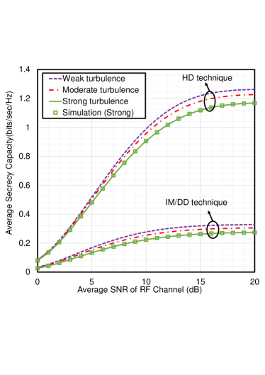
Figure 2: The ASC versus ${\omega}_{r}$ for selected values of $\alpha_{d},\beta_{d}$, and $r$ where $\alpha_{r}=\alpha_{v}=4$, $\mu_{r}=\mu_{v}=1$, $\eta_{r}=\eta_{v}{\approx}1$, $\Omega_{d}=g_{d}=2$, $u_{r}=10$ dB, and $\omega_{v}=0$ dB.

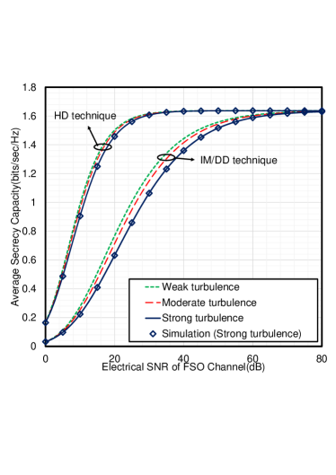
Figure 3: The ASC versus $u_{r}$ for selected values of $\alpha_{d}$, $\beta_{d}$, and $r$ where $\alpha_{r}=\alpha_{v}=4$, $\mu_{r}=\mu_{v}=1$, $\eta_{r}=\eta_{v}\approx 1$, $\Omega_{d}=g_{d}=2$, $\omega_{r}=10$ dB, and $\omega_{v}=0$ dB.

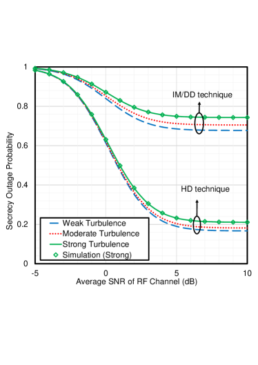
Figure 4: The SOP versus $\omega_{m}$ for selected values of $\alpha_{d}$, $\beta_{d}$, and $r$ where $\Omega_{d}=g_{d}=2$, $\varepsilon=6.7$, $\alpha_{r}=\alpha_{v}=4$, $\mu_{r}=\mu_{v}=1$, $\eta_{r}=\eta_{v}\approx 1$, $R_{s}=0.1$ bits/sec/Hz, $\omega_{v}=0$ dB, and $u_{r}=10$ dB.

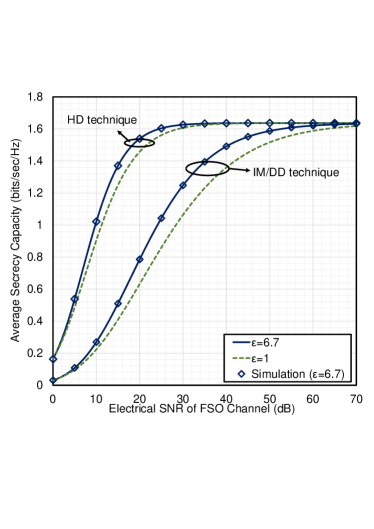
Figure 5: The ASC versus $u_{r}$ for selected values of $\varepsilon$ and $r$ where $\alpha_{d}=2.296$, $\beta_{d}=2$, $\eta_{r}=\eta_{v}\approx 1$, $\Omega_{d}=g_{d}=2$, $\omega_{r}=10$ dB, and $\omega_{v}=0$ dB.

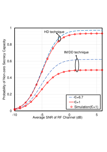
Figure 6: The PNSC versus $\omega_{r}$ for the selected values of $\varepsilon$ and $r$ where $\Omega_{d}=g_{d}=2$, $\alpha_{r}=\alpha_{v}=4$, $\eta_{r}=\eta_{v}\approx 1$, $\mu_{r}=\mu_{v}=1$, $\omega_{v}=-5$ dB, and $u_{r}=10$ dB.

The effects of atmospheric turbulence on the system performance are also demonstrated in Figs. 2, 3, and 4 where the system performance will be at its best for no or weak atmospheric turbulence condition and becomes vulnerable with the increasing amount of turbulence as proved in [68, 41, 69, 70, 67]. This characteristic is observed due to the fact that with increasing turbulence, the SNR at the receiver becomes smaller that in turn deteriorates the system security. The MC simulation demonstrates a close agreement with our analytical results, which point out the exactitude of the analytical expressions.

Pointing error signifies the misalignment between transmitter and receiver that causes huge data loss in FSO systems and it is an important factor that controls the integrity of FSO links. To evaluate the effect of the pointing error, the values of $\varepsilon$ have been appointed as $1$ and $6.7$ that corresponds to high and low pointing errors, respectively. As the FSO network depends on the LOS communication, the secrecy of the proposed system degrades with a higher pointing error between the transmitting and receiving aperture as demonstrated in Figs. 5 and 6. Similar results are also achieved in [19, 44, 39] that justify our results.

A comprehensive study on the effect of both pointing error and turbulence on the security of the proposed model is presented in Figs. 7 and 8 for PNSC and SOP, respectively. In both figures, the turbulence is varied for small and large pointing errors and it can be observed that the performance of the proposed system reduces at higher pointing error, as established in [39]. One can try to improve the system quality by decreasing the atmospheric turbulence but won’t be able to remedy the situation completely, as analyzed in Figs. 7 and 8, because the effect of pointing error is much higher than the turbulence created in the atmosphere. Hence, it is very important to maintain a lower pointing error for secure RF-FSO communications, regardless of the atmospheric turbulence conditions.

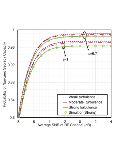
Figure 7: The PNSC versus $\omega_{r}$ for the selected values of $\alpha_{d}$, $\beta_{d}$, and $r$ where $\Omega_{d}=g_{d}=2$, $\alpha_{r}=\alpha_{v}=4$, $\mu_{r}=\mu_{v}=1$, $\eta_{r}=\eta_{v}\approx 1$, $\omega_{v}=-10$ dB, and $u_{r}=10$ dB.

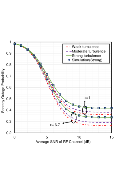
Figure 8: The SOP versus $\omega_{r}$ for selected values of $\alpha_{d}$, $\beta_{d}$, and $r$ where $\Omega_{d}=2$, $\alpha_{r}=\alpha_{v}=4$, $\mu_{r}=\mu_{v}=1$, $\eta_{r}=\eta_{v}\approx 1$, $g_{d}=2$, $R_{s}=0.1$ bits/sec/Hz, and $\omega_{v}=5$ dB.

Figure 9 demonstrates the effect of average SNR of the eavesdropper channel ($\omega_{v}$) plotted against $\omega_{r}$ on the ASC of this proposed work. It is clearly illustrated from the Fig. that with increasing values of $\omega_{v}$, a sharp decay occurs in the secrecy capacity of the system. The reason behind this is the increment in $\omega_{v}$ actually increases the quality of the eavesdropper channel and thus the eavesdropper gains unauthorized access to more data that compromises the secrecy of the transmitted data. The authors in [39, 71] have also deduced similar results.

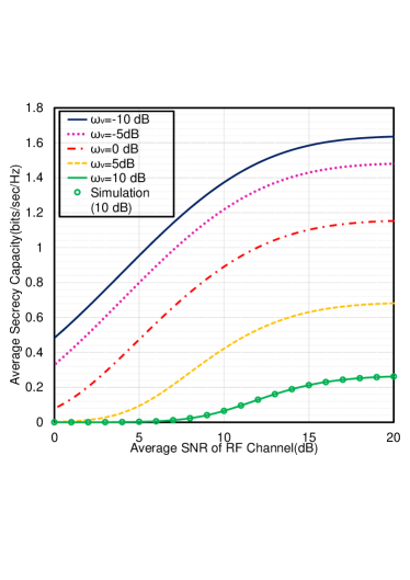
Figure 9: The ASC versus ${\omega}_{r}$ for selected values of $\omega_{v}$ where $\alpha_{r}=\alpha_{v}=4$, $\mu_{r}=\mu_{v}=1$, $\eta_{r}=\eta_{v}\approx 1$, $\alpha_{d}=2.296$, $\beta_{d}=2$, $r=1$, $\Omega_{d}=g_{d}=2$, and $u_{r}=10$ dB.

The effect of non-linearity along with the number of multipath clusters has a tremendous effect on the environmental fading through which the RF signal has to propagate towards the destination. The influence of these parameters on the proposed system is demonstrated in Figs. 10 and 11 considering variations in main channel and eavesdropper channel, respectively. Fig. 10 illustrates the security can be enhanced by increasing the value of $\alpha_{r}$ and $\mu_{r}$. The increment in $\alpha_{r}$ reduces the total non-linearity of the system that in turn reduces the environmental fading. On the other hand, with increasing values of $\mu_{r}$, total multipath clusters are increased that increases the possibility of achieving a better SNR at the relay, and thus security is increased. Similar analysis is displayed in Fig. 11 where these parameters for the eavesdropper channel are varied. We can observe that the security of the system reduces with increasing $\alpha_{v}$ and $\mu_{v}$ because their increment actually consolidates the eavesdropper channel that becomes able to steal more data from the legitimate RF channel. Same characteristics are also perceived in [53, 72, 38, 73]. We can observe that a SOP floor is reached in Fig. 10 that is due to the limitation of RF link rather than the FSO link.

Table 1: Generalization of the Proposed Model.

Envelope distribution	Parameters
($\alpha-\mu$)-Málaga	$\alpha_{r}=\alpha_{v}=4$, $\mu_{r}=\mu_{v}=1$, $g_{d}=2$, $\Omega_{d}=1$, $\rho=0$
($\eta-\mu$)-Málaga	$\alpha_{r}=\alpha_{v}=6$, $\mu_{r}=\mu_{v}=3$, $g_{d}=2$, $\Omega_{d}=4$, $\rho=0$
(Nakagami-$m$)-($\Gamma-\Gamma$)	$\alpha_{r}=\alpha_{v}=2$, $\mu_{r}=\mu_{v}=1$, $g_{d}=0$, $\Omega_{d}=1$, $\rho=1$
Rayeleigh-($\Gamma-\Gamma$)	$\alpha_{r}=\alpha_{v}=2$, $\mu_{r}=\mu_{v}=0.5$, $g_{d}=0$, $\Omega_{d}=1$, $\rho=1$
Weibull-Lognormal	$\alpha_{r}=\alpha_{v}=4$, $\mu_{r}=\mu_{v}=0.5$, $g_{d}=0.0001$, $\Omega_{d}=1.3265$, $\rho=0$

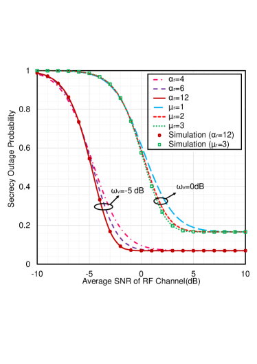
Figure 10: The SOP versus $\omega_{r}$ for selected values of $\alpha_{r}$, $\mu_{r}$, and $\omega_{v}$ where $\Omega_{d}=g_{d}=2$, $\alpha_{v}=4$, $\mu_{v}=1$, $\eta_{r}=\eta_{v}\approx 1$, $\varepsilon=1$, $R_{s}=0.1$ bits/sec/Hz, and $u_{r}=10$ dB.

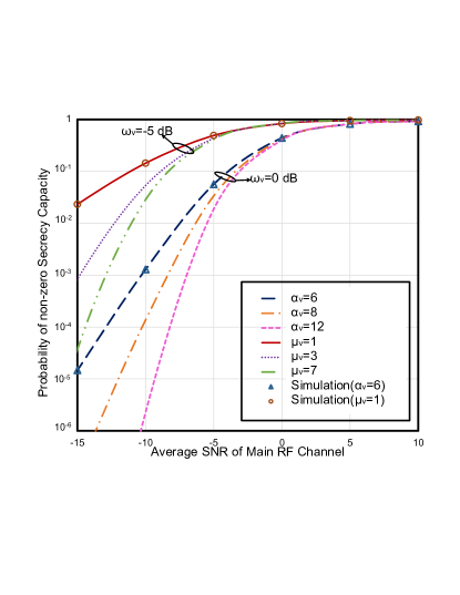
Figure 11: The PNSC versus $\omega_{r}$ for selected values of $\alpha_{v}$, $\mu_{v}$, and $\omega_{v}$ where $\Omega_{d}=g_{d}=2$, $\alpha_{r}=2$, $\mu_{r}=1$, $\eta_{r}=\eta_{v}\approx 1$, $\varepsilon=1$, $\alpha_{d}=8$, $\beta_{d}=4$, and $u_{r}=15$ dB.

The target secrecy rate ($R_{s}$), as defined earlier, is a threshold capacity that determines whether the instantaneous secrecy capacity of the transmitting signal is below or greater than this rate. For supreme secrecy, the instantaneous secrecy rate must be higher than the $R_{s}$. But with increasing $R_{s}$, the probability of the instantaneous secrecy capacity being higher than the $R_{s}$ becomes smaller. As a result, the secrecy outage of the system increases. This phenomenon is exhibited in Fig. 12 where SOP of the proposed system is plotted against ${\omega}_{r}$ for varying values of $R_{s}$. This same behaviour has also been observed in [53, 74].

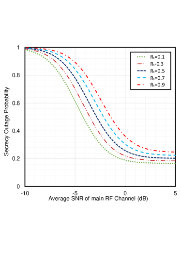
Figure 12: The SOP versus ${\omega}_{r}$ for selected values of $R_{s}$, where $\alpha_{r}=\alpha_{v}=4$, $\mu_{r}=\mu_{v}=1$, $\eta_{r}=\eta_{v}\approx 1$, $\alpha_{d}=8$, $\beta_{d}=4$, $r=1$, $\Omega_{d}=g_{d}=2$, $u_{r}=5$ dB, and $\omega_{v}=-5$ dB.

Special Cases of the Proposed Scenario:

As discussed earlier, the communications system proposed in this work considers generalized fading conditions at both RF and FSO link that enables this model to be applicable for a wide variety of fading scenarios. Figure 13 demonstrates a few well-known combinations of RF-FSO links that have been studied in some earlier works. Hence, by altering some parameter values (as given in Table 1) in our proposed work, we can analyze all these models that are previously studied in [36, 37, 41, 42] (considering the single antenna in [41, 42]) as well as many other combinations of RF-FSO hops. This prominent characteristic makes our analysis more unique and novel relative to others.

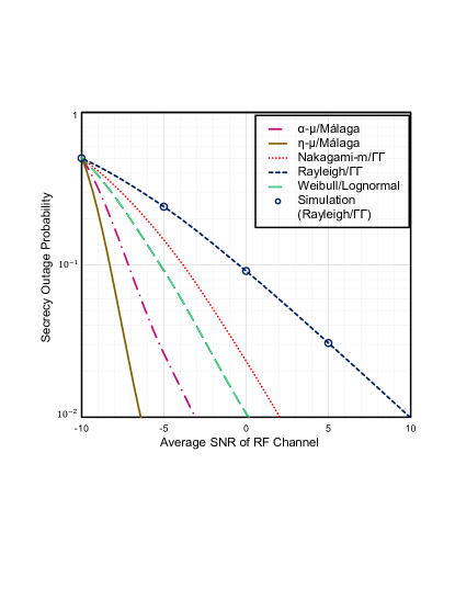
Figure 13: The SOP versus ${\omega}_{r}$ for selected values of $\alpha_{r}$, $\alpha_{v}$, $\mu_{r}$, $\mu_{v}$, $\rho$, $g_{d}$, and $\Omega_{d}$ where $\alpha_{d}=8$, $\beta_{d}=4$, $r=1$, $\eta_{r}=\eta_{v}\approx 1$, $u_{r}=20$ dB, and $\omega_{v}=-10$ dB.

5 Conclusion

This work deals with the mathematical modeling of a secure RF-FSO network considering a variable gain relaying scheme for $\alpha-\eta-\mu$ fading model at the RF hop and Málaga model at the FSO hop. The secrecy analysis of the proposed scenario has been performed via deriving the closed-form expressions for the performance metrics i.e. ASC, lower bound of SOP, and PNSC incorporating the adverse effects of the fading, pointing errors, and atmospheric turbulence for both HD and IM/DD techniques. We further corroborate the analytical results via MC simulations. As predicted, HD demonstrates superior secrecy performance than the IM/DD technique. Although both pointing errors and atmospheric turbulence are the reasons behind the degradation of the security, the effect of pointing error is far worse than the turbulence. Moreover, we focus on the generalization of the existing works incorporating more complicated composite channels such as $\alpha-\eta-\mu$ fading and unified Málaga turbulent models that will pave the way for the communication engineers to design more practical secure digital communication scenarios via exploiting the randomness of the wireless channels.

Appendix

Appendix A Proof of ASC

For mathematical simplification, we have considered $\tilde{\alpha_{r}}=\tilde{\alpha_{v}}=\tilde{\alpha}$. The final expressions of $\mathcal{S}_{1}$, $\mathcal{S}_{2}$, $\mathcal{S}_{3}$, and $\mathcal{S}_{4}$ are given below.

Calculation of $\mathcal{S}_{1}$:

Using the identities [75, Eqs. (8.4.3.1), (8.4.2.5),], (20a) can be given as

$$\mathcal{S}_{1}=\int_{0}^{\infty}\gamma^{\tilde{\alpha}t_{1}}G_{1,1}^{1,1}\left[\gamma\biggl{|}\begin{array}[]{c}0\\ 0\\ \end{array}\right]G_{0,1}^{1,0}\left[u_{2}\gamma^{\tilde{\alpha}}\biggl{|}\begin{array}[]{c}.\\ 0\\ \end{array}\right]d\gamma.$$ (31)

Now, applying [75, Eqs. (2.24.1.1),] in (31) and performing the integration, we obtain

$$\mathcal{S}_{1}=(2\pi)^{1-\tilde{\alpha}}G_{\tilde{\alpha},1+\tilde{\alpha}}^{1+\tilde{\alpha},\tilde{\alpha}}\left[u_{2}\biggl{|}\begin{array}[]{c}\Delta(\tilde{\alpha},-\tilde{\alpha}t_{1})\\ 0,\Delta(\tilde{\alpha},-\tilde{\alpha}t_{1})\\ \end{array}\right],$$ (34)

where $\Delta(a,b)=\frac{b}{a},\frac{b+1}{a},...,\frac{b+a-1}{a}$.

Calculation of $\mathcal{S}_{2}$:

We derive $\mathcal{S}_{2}$ by following the similar process as $\mathcal{S}_{1}$ and $\mathcal{S}_{2}$ can be expressed as

$$\mathcal{S}_{2} =\int_{0}^{\infty}\gamma^{\tilde{\alpha}\mathcal{T}}G_{1,1}^{1,1}\left[\gamma\biggl{|}\begin{array}[]{c}0\\ 0\\ \end{array}\right]G_{0,1}^{1,0}\left[\Im\gamma^{\tilde{\alpha}}\biggl{|}\begin{array}[]{c}.\\ 0\\ \end{array}\right]d\gamma$$ (39)

$$=(2\pi)^{1-\tilde{\alpha}}G_{\tilde{\alpha},1+\tilde{\alpha}}^{1+\tilde{\alpha},\tilde{\alpha}}\left[\Im\biggl{|}\begin{array}[]{c}\Delta(\tilde{\alpha},-\tilde{\alpha}\mathcal{T})\\ 0,\Delta(\tilde{\alpha},-\tilde{\alpha}\mathcal{T})\\ \end{array}\right],$$ (42)

where $\mathcal{T}=t_{1}+t_{2}$ and $\Im=u_{2}+q_{2}$.

Calculation of $\mathcal{S}_{3}$:

Utilizing the identities [75, Eqs. (8.4.3.1), (8.4.2.5),] in (20e), $\mathcal{S}_{3}$ can be expressed as

$$\mathcal{S}_{3} =\int_{0}^{\infty}\gamma^{\tilde{\alpha}t_{1}}G_{1,1}^{1,1}\left[\gamma\biggl{|}\begin{array}[]{c}0\\ 0\\ \end{array}\right]G_{0,1}^{1,0}\left[u_{2}\gamma^{\tilde{\alpha}}\biggl{|}\begin{array}[]{c}.\\ 0\\ \end{array}\right]G_{r+1,3r+1}^{3r,1}\left[\frac{F\gamma}{u_{r}}\biggl{|}\begin{array}[]{c}1,l_{1}\\ l_{2},0\\ \end{array}\right]d\gamma.$$ (49)

For deriving the closed form expression of $\mathcal{S}_{3}$, we must integrate (49) within the limit $0$ to $\infty$ that is mathematically intractable. So, for obtaining $\mathcal{S}_{3}$ in closed-form, Meijer’s $G$ function terms are converted into Fox’s $H$ functions utilizing [75, Eqs. (8.3.2.21),] as

$$\mathcal{S}_{3} =\int_{0}^{\infty}\gamma^{\tilde{\alpha}t_{1}}H_{1,1}^{1,1}\left[\gamma\biggl{|}\begin{array}[]{c}{[}0,1{]}\\ {[}0,1{]}\\ \end{array}\right]H_{0,1}^{1,0}\left[u_{2}\gamma^{\tilde{\alpha}}\biggl{|}\begin{array}[]{c}.\\ {[}0,1{]}\\ \end{array}\right]H_{r+1,3r+1}^{3r,1}\left[\frac{F\gamma}{u_{r}}\biggl{|}\begin{array}[]{c}{[}1,1{]},{[}l_{1},1{]}\\ {[}l_{2},1{]},{[}0,1{]}\\ \end{array}\right]d\gamma.$$ (56)

Again, for mathematical simplification, we assume $x=\gamma^{\tilde{\alpha}}$. So, (56) can be expressed as

$$\mathcal{S}_{3} =\frac{1}{\tilde{\alpha}}\int_{0}^{\infty}x^{\mathcal{M}_{1}-1}H_{0,1}^{1,0}\left[u_{2}x\biggl{|}\begin{array}[]{c}.\\ {[}0,1{]}\\ \end{array}\right]H_{1,1}^{1,1}\left[x^{\frac{1}{\tilde{\alpha}}}\biggl{|}\begin{array}[]{c}{[}0,1{]}\\ {[}0,1{]}\\ \end{array}\right]H_{r+1,3r+1}^{3r,1}\left[\frac{Fx^{\frac{1}{\tilde{\alpha}}}}{u_{r}}\biggl{|}\begin{array}[]{c}{[}1,1{]},{[}l_{1},1{]}\\ {[}l_{2},1{]},{[}0,1{]}\\ \end{array}\right]dx.$$ (63)

Now utilizing [76, Eq. (2.3),], [36, Eq. (3),], the final expression of $\mathcal{S}_{3}$ is derived as

$$\mathcal{S}_{3} =\frac{1}{\tilde{\alpha}{u_{2}}^{\mathcal{M}_{1}}}H_{1,0;1,1;r+1,3r+1}^{1,0;1,1;3r,1}\left[\begin{array}[]{c}{[}1-\mathcal{M}_{1};\frac{1}{\tilde{\alpha}},\frac{1}{\tilde{\alpha}}{]}\\ -\\ \end{array}\biggl{|}\begin{array}[]{c}{[}0,1{]}\\ {[}0,1{]}\\ \end{array}\biggl{|}\begin{array}[]{c}{[}1,1{]},{[}l_{1},1{]}\\ {[}l_{2},1{]},{[}0,1{]}\\ \end{array}\biggl{|}\frac{1}{{u_{2}}^{\frac{1}{\tilde{\alpha}}}},\frac{F}{u_{r}{u_{2}}^{\frac{1}{\tilde{\alpha}}}}\right],$$ (70)

where $\mathcal{M}_{1}=\frac{1}{\tilde{\alpha}}+t_{1}$, $H_{m1,n1:m2,n2:m3,q3}^{p1,q1:p2,q2:p3,q3}[.]$ is the extended generalized bivariate Fox’s $H$ function.

Calculation of $\mathcal{S}_{4}$:

Similar to $\mathcal{S}_{3}$, $\mathcal{S}_{4}$ is obtained as

$$\mathcal{S}_{4} =\int_{0}^{\infty}\gamma^{\tilde{\alpha}\mathcal{T}}G_{1,1}^{1,1}\left[\gamma\biggl{|}\begin{array}[]{c}0\\ 0\\ \end{array}\right]G_{0,1}^{1,0}\left[\Im\gamma^{\tilde{\alpha}}\biggl{|}\begin{array}[]{c}.\\ 0\\ \end{array}\right]G_{r+1,3r+1}^{3r,1}\left[\frac{F\gamma}{u_{r}}\biggl{|}\begin{array}[]{c}1,l_{1}\\ l_{2},0\\ \end{array}\right]d\gamma$$ (77)

$$=\int_{0}^{\infty}\gamma^{\tilde{\alpha}\mathcal{T}}H_{1,1}^{1,1}\left[\gamma\biggl{|}\begin{array}[]{c}{[}0,1{]}\\ {[}0,1{]}\\ \end{array}\right]H_{0,1}^{1,0}\left[\Im\gamma^{\tilde{\alpha}}\biggl{|}\begin{array}[]{c}.\\ {[}0,1{]}\\ \end{array}\right]H_{r+1,3r+1}^{3r,1}\left[\frac{F\gamma}{u_{r}}\biggl{|}\begin{array}[]{c}{[}1,1{]},{[}l_{1},1{]}\\ {[}l_{2},1{]},{[}0,1{]}\\ \end{array}\right]d\gamma$$ (84)

$$=\frac{1}{\tilde{\alpha}}\int_{0}^{\infty}x^{\mathcal{M}_{2}-1}H_{0,1}^{1,0}\left[\Im x\biggl{|}\begin{array}[]{c}.\\ {[}0,1{]}\\ \end{array}\right]H_{1,1}^{1,1}\left[x^{\frac{1}{\tilde{\alpha}}}\biggl{|}\begin{array}[]{c}{[}0,1{]}\\ {[}0,1{]}\\ \end{array}\right]\times H_{r+1,3r+1}^{3r,1}\left[\frac{Fx^{\frac{1}{\tilde{\alpha}}}}{u_{r}}\biggl{|}\begin{array}[]{c}{[}1,1{]},{[}l_{1},1{]}\\ {[}l_{2},1{]},{[}0,1{]}\\ \end{array}\right]dx$$ (91)

$$=\frac{1}{\tilde{\alpha}{\Im}^{\mathcal{M}_{2}}}H_{1,0;1,1;r+1,3r+1}^{1,0;1,1;3r,1}\left[\begin{array}[]{c}{[}1-\mathcal{M}_{2};\frac{1}{\tilde{\alpha}},\frac{1}{\tilde{\alpha}}{]}\\ -\\ \end{array}\biggl{|}\begin{array}[]{c}{[}0,1{]}\\ {[}0,1{]}\\ \end{array}\biggl{|}\begin{array}[]{c}{[}1,1{]},{[}l_{1},1{]}\\ {[}l_{2},1{]},{[}0,1{]}\\ \end{array}\biggl{|}\biggl{|}\frac{1}{{\Im}^{\frac{1}{\tilde{\alpha}}}},\frac{F}{u_{r}{\Im}^{\frac{1}{\tilde{\alpha}}}}\right],$$ (98)

where $\mathcal{M}_{2}=\frac{1}{\tilde{\alpha}}+\mathcal{T}$.

Appendix B Proof of SOP

Plugging (14) and (16) into (22) leads to

$$P_{out}^{L}(R_{s}) =1-\sum_{N_{1}=0}^{\infty}\sum_{N_{2}=0}^{\infty}\sum_{t_{1}=0}^{W_{1}-1}u_{4}q_{2}\theta^{\tilde{\alpha_{r}}t_{1}}\int_{0}^{\infty}e^{-(u_{2}\theta\gamma^{\tilde{\alpha_{r}}}+q_{2}\gamma^{\tilde{\alpha_{v}}})}$$

$$\times{\gamma}^{q_{3}+\tilde{\alpha_{r}}t_{1}}\biggl{(}1-\sigma\sum_{\tilde{m}_{d}=1}^{\beta_{d}}c_{d}G_{r+1,3r+1}^{3r,1}\left[\frac{F}{u_{r}}(\theta\gamma)\biggl{|}\begin{array}[]{c}1,l_{1}\\ l_{2},0\\ \end{array}\right]\biggl{)}d\gamma.$$ (101)

Here, for mathematical tractability, we consider $\tilde{\alpha_{r}}=\tilde{\alpha_{v}}=\tilde{\alpha}$.

Calculation of $\mathcal{H}_{1}$:

Using [56, Eq. (3.326.2),], $\mathcal{H}_{1}$ is expressed as

$$\mathcal{H}_{1} =\int_{0}^{\infty}{\gamma}^{q_{3}+\tilde{\alpha}t_{1}}e^{-\kappa\gamma^{\tilde{\alpha}}}d\gamma={\frac{\Gamma(\mathcal{Z}_{1})}{\tilde{\alpha}{\kappa}^{\mathcal{Z}_{1}}}},$$ (102)

where $\mathcal{Z}_{1}=\frac{q_{3}+\tilde{\alpha_{r}}t_{1}+1}{\tilde{\alpha}}$ and $\kappa=u_{2}\theta+q_{2}$.

Calculation of $\mathcal{H}_{2}$:

$\mathcal{H}_{2}$ in (23) is given as

$$\mathcal{H}_{2}=\int_{0}^{\infty}{\gamma}^{q_{3}+\tilde{\alpha}t_{1}}e^{-\kappa\gamma^{\tilde{\alpha}}}G_{r+1,3r+1}^{3r,1}\left[\frac{F}{u_{r}}(\theta\gamma)\biggl{|}\begin{array}[]{c}1,l_{1}\\ l_{2},0\\ \end{array}\right]d\gamma.$$ (105)

Letting $I=\gamma^{\tilde{\alpha}}$ and utilizing [75, Eqs. (8.4.3.1) and (2.24.1.1),], $\mathcal{H}_{2}$ can be expressed as

$$\mathcal{H}_{2}={\frac{1}{\tilde{\alpha}}}\int_{0}^{\infty}I^{\mathcal{Z}_{1}-1}e^{-\kappa I}G_{r+1,3r+1}^{3r,1}\left[\frac{F\theta}{u_{r}}I^{\frac{1}{\tilde{\alpha}}}\biggl{|}\begin{array}[]{c}1,l_{1}\\ l_{2},0\\ \end{array}\right]dI$$ (108)

$$={\frac{(2\pi)^{(1-\tilde{\alpha})r}}{{\kappa}^{\mathcal{Z}_{1}}\tilde{\alpha}^{1-\mathcal{Z}_{2}}}}G_{\tilde{\alpha}r+\tilde{\alpha}+1,3\tilde{\alpha}r+\tilde{\alpha}}^{3\tilde{\alpha}r,\tilde{\alpha}+1}\left[\frac{(F\theta)^{\tilde{\alpha}}}{{u_{r}}^{\tilde{\alpha}}\kappa{\tilde{\alpha}}^{2\tilde{\alpha}r}}\biggl{|}\begin{array}[]{c}x_{1},1-\mathcal{Z}_{1},x_{2}\\ x_{3},0\\ \end{array}\right],$$ (111)

where $\mathcal{Z}_{2}=\Delta(r,\varepsilon^{2})+\Delta(r,\alpha_{d})+\Delta(r,\tilde{m}_{d})-\Delta(r,\varepsilon^{2}+1)-r$, $x_{1}=\Delta(\tilde{\alpha},1)$, $x_{2}=\Delta(\tilde{\alpha},l_{1})$, and $x_{3}=\Delta(\tilde{\alpha},l_{2})$.

References

- [1] J. G. Andrews, S. Buzzi, W. Choi, S. V. Hanly, A. Lozano, A. C. Soong, and J. C. Zhang, “What will 5G be?” \JournalTitleIEEE Journal on selected areas in communications 32, 1065–1082 (2014).
- [2] S. Dang, O. Amin, B. Shihada, and M.-S. Alouini, “What should 6G be?” \JournalTitleNature Electronics 3, 20–29 (2020).
- [3] S. Seo, D.-E. Ko, and J.-M. Chung, “Combined time bound optimization of control, communication, and data processing for FSO-based 6G UAV aerial networks,” \JournalTitleETRI Journal 42, 700–711 (2020).
- [4] S. H. Islam, A. S. M. Badrudduza, S. R. Islam, F. I. Shahid, I. S. Ansari, M. K. Kundu, and H. Yu, “Impact of correlation and pointing error on secure outage performance over arbitrary correlated Nakagami- and M-turbulent fading mixed RF-FSO channel,” \JournalTitleIEEE Photonics Journal (2021).
- [5] S. Sharma, A. Madhukumar, and R. Swaminathan, “Effect of pointing errors on the performance of hybrid FSO/RF networks,” \JournalTitleIEEE Access 7, 131418–131434 (2019).
- [6] S. Anees and M. R. Bhatnagar, “Performance of an amplify-and-forward dual-hop asymmetric RF-FSO communication system,” \JournalTitleJournal of Optical Communications and Networking 7, 124–135 (2015).
- [7] I. S. Ansari, F. Yilmaz, and M.-S. Alouini, “Impact of pointing errors on the performance of mixed RF/FSO dual-hop transmission systems,” \JournalTitleIEEE Wireless Communications Letters 2, 351–354 (2013).
- [8] A. Upadhya, V. K. Dwivedi, and G. Singh, “Relay-aided free-space optical communications using - distribution over atmospheric turbulence channels with misalignment errors,” \JournalTitleOptics Communications 416, 117–124 (2018).
- [9] I. S. Ansari, M. M. Abdallah, M. Alouini, and K. A. Qaraqe, “Outage analysis of asymmetric RF-FSO systems,” in 2016 IEEE 84th Vehicular Technology Conference (VTC-Fall), (2016), pp. 1–6.
- [10] S. Anees and M. R. Bhatnagar, “Performance evaluation of decode-and-forward dual-hop asymmetric radio frequency-free space optical communication system,” \JournalTitleIET Optoelectronics 9, 232–240 (2015).
- [11] Y. Wang, P. Wang, X. Liu, and T. Cao, “On the performance of dual-hop mixed RF/FSO wireless communication system in urban area over aggregated exponentiated Weibull fading channels with pointing errors,” \JournalTitleOptics Communications 410, 609–616 (2018).
- [12] I. S. Ansari, M. M. Abdallah, M. Alouini, and K. A. Qaraqe, “Outage performance analysis of underlay cognitive RF and FSO wireless channels,” in 2014 3rd International Workshop in Optical Wireless Communications (IWOW), (2014), pp. 6–10.
- [13] I. S. Ansari, M. M. Abdallah, M. Alouini, and K. A. Qaraqe, “A performance study of two hop transmission in mixed underlay RF and FSO fading channels,” in 2014 IEEE Wireless Communications and Networking Conference (WCNC), (2014), pp. 388–393.
- [14] F. S. Al-Qahtani, A. H. A. El-Malek, I. S. Ansari, R. M. Radaydeh, and S. A. Zummo, “Outage analysis of mixed underlay cognitive RF MIMO and FSO relaying with interference reduction,” \JournalTitleIEEE Photonics Journal 9, 1–22 (2017).
- [15] E. Erdogan, “On the performance of cognitive underlay RF/FSO communication systems with limited feedback,” \JournalTitleOptics Communications 444, 87–92 (2019).
- [16] I. A. Alimi, P. P. Monteiro, and A. L. Teixeira, “Analysis of multiuser mixed RF/FSO relay networks for performance improvements in cloud computing-based radio access networks (cc-rans),” \JournalTitleOptics Communications 402, 653–661 (2017).
- [17] X. Yi, C. Shen, P. Yue, Y. Wang, and Q. Ao, “Performance of decode-and-forward mixed RF/FSO system over - shadowed and exponentiated Weibull fading,” \JournalTitleOptics Communications 439, 103–111 (2019).
- [18] X. Yi, Q. Ao, P. Yue, C. Shen, Y. Wang, and P. Zhao, “Performance analysis for mixed - shadowed and exponentiated Weibull distributed dual-hop system with multiuser diversity in c-ran,” \JournalTitleOptics Communications 460, 124926 (2020).
- [19] E. Zedini, I. S. Ansari, and M.-S. Alouini, “Performance analysis of mixed Nakagami- and Gamma-Gamma dual-hop FSO transmission systems,” \JournalTitleIEEE Photonics Journal 7, 1–20 (2014).
- [20] J. Zhao, S.-H. Zhao, W.-H. Zhao, Y. Liu, and X. Li, “Performance of mixed RF/FSO systems in exponentiated Weibull distributed channels,” \JournalTitleOptics Communications 405, 244–252 (2017).
- [21] V. K. Tonk, A. Upadhya, P. K. Yadav, and V. K. Dwivedi, “Mixed mud-RF/FSO two way dcode and forward relaying networks in the presence of co-channel interference,” \JournalTitleOptics Communications 464, 125415 (2020).
- [22] J. Feng and X. Zhao, “Performance analysis of mixed RF/FSO systems with STBC users,” \JournalTitleOptics Communications 381, 244–252 (2016).
- [23] K. O. Odeyemi and P. A. Owolawi, “On the performance of transmit antenna selection in multiuser asymmetric RF/FSO system under generalized order user scheduling,” \JournalTitleOptik 197, 163102 (2019).
- [24] Z. Wang, W. Shi, and W. Liu, “Performance analysis of mixed RF/FSO system with spatial diversity,” \JournalTitleOptics Communications 443, 230–237 (2019).
- [25] A. Asgari-Forooshani, M. Aghabozorgi, E. Soleimani-Nasab, and M. A. Khalighi, “Performance analysis of mixed RF/FSO cooperative systems with wireless power transfer,” \JournalTitlePhysical Communication 33, 187–198 (2019).
- [26] L. Han, H. Jiang, Y. You, and Z. Ghassemlooy, “On the performance of a mixed RF/MIMO FSO variable gain dual-hop transmission system,” \JournalTitleOptics Communications 420, 59–64 (2018).
- [27] L. Chen and W. Wang, “Multi-diversity combining and selection for relay-assisted mixed RF/FSO system,” \JournalTitleOptics Communications 405, 1–7 (2017).
- [28] M. Torabi and R. Effatpanahi, “Performance analysis of hybrid RF–FSO systems with amplify-and-forward selection relaying,” \JournalTitleOptics Communications 434, 80–90 (2019).
- [29] Y. Zhang, X. Wang, S.-H. Zhao, J. Zhao, and B.-Y. Deng, “On the performance of 2 2 DF relay mixed RF/FSO airborne system over exponentiated Weibull fading channel,” \JournalTitleOptics Communications 425, 190–195 (2018).
- [30] E. Erdogan, “Joint user and relay selection for relay-aided RF/FSO systems over exponentiated Weibull fading channels,” \JournalTitleOptics Communications 436, 209–215 (2019).
- [31] K. O. Odeyemi and P. A. Owolawi, “Selection combining hybrid FSO/RF systems over generalized induced-fading channels,” \JournalTitleOptics Communications 433, 159–167 (2019).
- [32] Z. Jing, Z. Shang-hong, Z. Wei-hu, and C. Ke-fan, “Performance analysis for mixed FSO/RF Nakagami- and exponentiated Weibull dual-hop airborne systems,” \JournalTitleOptics Communications 392, 294–299 (2017).
- [33] M. A. Amirabadi and V. T. Vakili, “Performance of a relay-assisted hybrid FSO/RF communication system,” \JournalTitlePhysical Communication 35, 100729 (2019).
- [34] M. A. Amirabadi and V. T. Vakili, “On the performance of a multi-user multi-hop hybrid FSO/RF communication system,” \JournalTitleOptics Communications 444, 172–183 (2019).
- [35] B. Van Nguyen, H. Jung, and K. Kim, “Physical layer security schemes for full-duplex cooperative systems: State of the art and beyond,” \JournalTitleIEEE Communications Magazine 56, 131–137 (2018).
- [36] H. Lei, Z. Dai, I. S. Ansari, K.-H. Park, G. Pan, and M.-S. Alouini, “On secrecy performance of mixed RF-FSO systems,” \JournalTitleIEEE Photonics Journal 9, 1–14 (2017).
- [37] L. Yang, T. Liu, J. Chen, and M.-S. Alouini, “Physical-layer security for mixed and -distribution dual-hop RF/FSO systems,” \JournalTitleIEEE Transactions on Vehicular Technology 67, 12427–12431 (2018).
- [38] N. A. Sarker, A. Badrudduza, S. R. Islam, S. H. Islam, I. S. Ansari, M. K. Kundu, M. F. Samad, M. B. Hossain, and H. Yu, “Secrecy performance analysis of mixed hyper-Gamma and Gamma-Gamma cooperative relaying system,” \JournalTitleIEEE Access 8, 131273–131285 (2020).
- [39] S. H. Islam, A. Badrudduza, S. R. Islam, F. I. Shahid, I. S. Ansari, M. K. Kundu, S. K. Ghosh, M. B. Hossain, A. S. Hosen, and G. H. Cho, “On secrecy performance of mixed generalized Gamma and Málaga RF-FSO variable gain relaying channel,” \JournalTitleIEEE Access 8, 104127–104138 (2020).
- [40] H. Lei, H. Luo, K.-H. Park, I. S. Ansari, W. Lei, G. Pan, and M.-S. Alouini, “On secure mixed RF-FSO systems with TAS and imperfect CSI,” \JournalTitleIEEE Transactions on Communications 68, 4461–4475 (2020).
- [41] H. Lei, H. Luo, K.-H. Park, Z. Ren, G. Pan, and M.-S. Alouini, “Secrecy outage analysis of mixed RF-FSO systems with channel imperfection,” \JournalTitleIEEE Photonics Journal 10, 1–13 (2018).
- [42] A. H. Abd El-Malek, A. M. Salhab, S. A. Zummo, and M.-S. Alouini, “Security-reliability trade-off analysis for multiuser SIMO mixed RF/FSO relay networks with opportunistic user scheduling,” \JournalTitleIEEE Transactions on Wireless Communications 15, 5904–5918 (2016).
- [43] A. H. Abd El-Malek, A. M. Salhab, S. A. Zummo, and M.-S. Alouini, “Effect of rf interference on the security-reliability tradeoff analysis of multiuser mixed RF/FSO relay networks with power allocation,” \JournalTitleJournal of Lightwave Technology 35, 1490–1505 (2017).
- [44] K. O. Odeyemi and P. A. Owolawi, “Physical layer security in mixed RF/FSO system under multiple eavesdroppers collusion and non-collusion,” \JournalTitleOptical and Quantum Electronics 50, 1–19 (2018).
- [45] K. O. Odeyemi and P. A. Owolawi, “Security outage performance of partial relay selection in af mixed RF/FSO system with outdated channel state information,” \JournalTitleTransactions on Emerging Telecommunications Technologies 30, e3555 (2019).
- [46] I. S. Ansari, F. Yilmaz, and M. Alouini, “On the sum of squared - random variates with application to the performance of wireless communication systems,” in 2013 IEEE 77th Vehicular Technology Conference (VTC Spring), (2013), pp. 1–6.
- [47] I. S. Ansari and M. Alouini, “On the performance analysis of digital communications over Weibull-Gamma channels,” in 2015 IEEE 81st Vehicular Technology Conference (VTC Spring), (2015), pp. 1–7.
- [48] I. S. Ansari, “Composite and cascaded generalized- fading channel modeling and their diversity and performance analysis,” (2010).
- [49] J. M. Moualeu, D. B. da Costa, W. Hamouda, U. S. Dias, and R. A. de Souza, “Physical layer security over -- and -- fading channels,” \JournalTitleIEEE Transactions on Vehicular Technology 68, 1025–1029 (2018).
- [50] O. S. Badarneh, “Error rate analysis of -ary phase shift keying in fading channels subject to additive Laplacian noise,” \JournalTitleIEEE Communications Letters 19, 1253–1256 (2015).
- [51] I. S. Ansari, M. Alouini, and J. Cheng, “On the capacity of FSO links under Lognormal and Rician-Lognormal turbulences,” in 2014 IEEE 80th Vehicular Technology Conference (VTC2014-Fall), (2014), pp. 1–6.
- [52] I. S. Ansari and M. Alouini, “Asymptotic ergodic capacity analysis of composite Lognormal shadowed channels,” in 2015 IEEE 81st Vehicular Technology Conference (VTC Spring), (2015), pp. 1–5.
- [53] H. A. B. Salameh, L. Mahdawi, A. Musa, and F. H. Tha’er, “End-to-end performance analysis with decode-and-forward relays in multihop wireless systems over fading channels,” \JournalTitleIEEE Systems Journal 14, 84–92 (2019).
- [54] S. Arya and Y.-H. Chung, “Multiuser interference-limited petahertz wireless communications over Málaga fading channels,” \JournalTitleIEEE Access 8, 137356–137369 (2020).
- [55] M. Abramowitz, I. A. Stegun et al., Handbook of mathematical functions: with formulas, graphs, and mathematical tables, vol. 55 (National bureau of standards Washington, DC, 1972).
- [56] I. S. Gradshteyn and I. M. Ryzhik, Table of integrals, series, and products (Academic press, 2014).
- [57] I. S. Ansari, F. Yilmaz, and M.-S. Alouini, “Performance analysis of free-space optical links over Málaga () turbulence channels with pointing errors,” \JournalTitleIEEE Transactions on Wireless Communications 15, 91–102 (2015).
- [58] M. J. Saber and A. Keshavarz, “On secrecy performance of mixed Nakagami- and Málaga RF/FSO variable gain relaying system,” in Electrical Engineering (ICEE), Iranian Conference on, (IEEE, 2018), pp. 354–357.
- [59] A. D. Wyner, “The wire-tap channel,” \JournalTitleBell system technical journal 54, 1355–1387 (1975).
- [60] A. H. A. El-Malek, A. M. Salhab, S. A. Zummo, and M.-S. Alouini, “Physical layer security enhancement in multiuser mixed RF/FSO relay networks under RF interference,” in 2017 IEEE Wireless Communications and Networking Conference (WCNC), (IEEE, 2017), pp. 1–6.
- [61] P. V. Trinh, T. C. Thang, and A. T. Pham, “Mixed mmwave RF/FSO relaying systems over generalized fading channels with pointing errors,” \JournalTitleIEEE Photonics Journal 9, 1–14 (2016).
- [62] M. J. Saber, A. Keshavarz, J. Mazloum, A. M. Sazdar, and M. J. Piran, “Physical-layer security analysis of mixed SIMO SWIPT RF and FSO fixed-gain relaying systems,” \JournalTitleIEEE Systems Journal 13, 2851–2858 (2019).
- [63] H. Lei, Z. Dai, K.-H. Park, W. Lei, G. Pan, and M.-S. Alouini, “Secrecy outage analysis of mixed RF-FSO downlink swipt systems,” \JournalTitleIEEE Transactions on Communications 66, 6384–6395 (2018).
- [64] J. Vellakudiyan, V. Palliyembil, I. S. Ansari, P. Muthuchidambaranathan, and K. A. Qaraqe, “Performance analysis of the decode-and-forward relay-based RF-FSO communication system in the presence of pointing errors,” \JournalTitleIET Signal Processing 13, 480–485 (2019).
- [65] E. Balti and M. Guizani, “Mixed RF/FSO cooperative relaying systems with co-channel interference,” \JournalTitleIEEE Transactions on Communications 66, 4014–4027 (2018).
- [66] E. Balti, M. Guizani, B. Hamdaoui, and B. Khalfi, “Aggregate hardware impairments over mixed RF/FSO relaying systems with outdated CSI,” \JournalTitleIEEE Transactions on Communications 66, 1110–1123 (2017).
- [67] V. Palliyembil, J. Vellakudiyan, P. Muthuchidamdaranathan, and T. A. Tsiftsis, “Capacity and outage probability analysis of asymmetric dual-hop RF–FSO communication systems,” \JournalTitleIET Communications 12, 1979–1983 (2018).
- [68] K. O. Odeyemi, P. A. Owolawi, and O. O. Olakanmi, “Secrecy performance of cognitive underlay hybrid RF/FSO system under pointing errors and link blockage impairments,” \JournalTitleOptical and Quantum Electronics 52, 1–16 (2020).
- [69] D. R. Pattanayak, V. K. Dwivedi, and V. Karwal, “Physical layer security of a two way relay based mixed FSO/RF network in the presence of multiple eavesdroppers,” \JournalTitleOptics Communications 463, 125429 (2020).
- [70] J. Hu, Z. Zhang, J. Dang, L. Wu, and G. Zhu, “Performance of decode-and-forward relaying in mixed Beaulieu-Xie and dual-hop transmission systems with digital coherent detection,” \JournalTitleIEEE Access 7, 138757–138770 (2019).
- [71] A. Badrudduza, M. Sarkar, and M. Kundu, “Enhancing security in multicasting through correlated Nakagami- fading channels with opportunistic relaying,” \JournalTitlePhysical Communication 43, 101177 (2020).
- [72] O. S. Badarneh and M. S. Aloqlah, “Performance analysis of digital communication systems over -- fading channels,” \JournalTitleIEEE Transactions on Vehicular Technology 65, 7972–7981 (2015).
- [73] J. Gupta, V. K. Dwivedi, and V. Karwal, “On the performance of RF-FSO system over Rayleigh and /inverse Gaussian fading environment,” \JournalTitleIEEE Access 6, 4186–4198 (2018).
- [74] A. Badrudduza, M. Ibrahim, S. R. Islam, M. S. Hossen, M. K. Kundu, I. S. Ansari, and H. Yu, “Security at the physical layer over GG fading and mEGG turbulence induced RF-UOWC mixed system,” \JournalTitleIEEE Access 9, 18123–18136 (2021).
- [75] A. P. Prudnikov, Y. A. Brychkov, O. I. Marichev, and R. H. Romer, Integrals and series (American Association of Physics Teachers, 1988).
- [76] P. Mittal and K. Gupta, “An integral involving generalized function of two variables,” in Proceedings of the Indian academy of sciences-section A, vol. 75 (Springer, 1972), pp. 117–123.