Temperature Damping of Magneto-Intersubband Resistance Oscillations in Magnetically Entangled Subbands

Abstract

Magneto-intersubband resistance oscillations (MISO) of highly mobile 2D electrons in symmetric GaAs quantum wells with two populated subbands are studied in magnetic fields tilted from the normal to the 2D electron layer at different temperatures $\displaystyle T$. Decrease of MISO amplitude with temperature increase is observed. At moderate tilts the temperature decrease of MISO amplitude is consistent with decrease of Dingle factor due to reduction of quantum electron lifetime at high temperatures. At large tilts new regime of strong MISO suppression with the temperature is observed. Proposed model relates this suppression to magnetic entanglement between subbands, leading to beating in oscillating density of states. The model yields corresponding temperature damping factor: $\displaystyle A_{MISO}(T)=X/\sinh(X)$, where $\displaystyle X=2\pi^{2}kT\delta f$ and $\displaystyle\delta f$ is difference frequency of oscillations of density of states in two subbands. This factor is in agreement with experiment. Fermi liquid enhancement of MISO amplitude is observed.

I Introduction

The orbital quantization of electron trajectories and spectrum in magnetic fields significantly affects the electron transport in condensed materials^{1; 2; 3}. Shubnikov-de Haas (SdH) resistance oscillations¹ and Quantum Hall Effect (QHE)⁴ are remarkable effects of the orbital quantization. These effects occur at a temperature, $\displaystyle T$, which is less than the cyclotron energy, $\displaystyle\Delta_{c}=\hbar\omega_{c}$, separating Landau levels. Here $\displaystyle\omega_{c}$ is the cyclotron frequency. At high temperatures, $\displaystyle kT>\hbar\omega_{c}$, both SdH oscillations and QHE are absent due to a spectral averaging of the oscillating density of states (DOS) in the energy interval, $\displaystyle\delta\epsilon\approx kT$, in a vicinity of Fermi energy, $\displaystyle\epsilon_{F}$.

At the high temperatures, $\displaystyle kT>\hbar\omega_{c}$, electron systems with multiple populated subbands continue to exhibit quantum resistance oscillations.^{5; 6; 7; 8; 9; 10} These magneto-inter-subband oscillations (MISO) of the resistance are due to an alignment between Landau levels from different subbands $\displaystyle i$ and $\displaystyle j$ with corresponding energies $\displaystyle E_{i}$ and $\displaystyle E_{j}$ at the bottom of the subbands. Resistance maxima occur at magnetic fields in which the gap between the bottoms of the subbands, $\displaystyle\Delta_{ij}=E_{i}-E_{j}$, is a multiple of the Landau level spacing: $\displaystyle\Delta_{ij}=k\cdot\hbar\omega_{c}$, where $\displaystyle k$ is an integer ^{11; 12; 13; 14; 15}. At this condition Landau levels of two subbands overlap and the electron elastic scattering on impurities is enhanced due to the possibility of electron transitions between the overlapped quantum levels of $\displaystyle i$-th and $\displaystyle j$-th subbands. At magnetic fields corresponding to the condition $\displaystyle\Delta_{ij}=(k+1/2)\cdot\hbar\omega_{c}$ the intersubband electron scattering is suppressed since the quantum levels of two subbands are misaligned. The spectral overlap between two subbands oscillates with the magnetic field and leads to MISO, which are periodic in the inverse magnetic field.

Recently we have studied transport properties of high quality GaAs quantum wells with two populated subbands in a tilted magnetic fields.¹⁶ The goals of that study were to detect effects of the spin (Zeeman) splitting on MISO, which has not been seen before as well as to investigate the effect of the spin splitting on quantum positive magnetoresistance (QPMR)^{17; 18; 19; 20} in a 2D system with two populated subbands . These experiments have demonstrated a significant reduction of the QPMR with the application of the in-plane magnetic field, which was in good agreement with the modification of the electron spectrum via Zeeman effect with g-factor $\displaystyle g\approx$0.43$\displaystyle\pm$0.07. MISO also have a strong reduction of the magnitude with the in-plane magnetic field. However in contrast to the QPMR, the MISO reduction is found to be predominantly related to a modification of the electron spectrum via a magnetic entanglement of two subbands, induced by the in-plane magnetic field.¹⁶

In zero magnetic field the electron motion in a quantum well can be separated on two independent parts: the lateral motion along the 2D layer and the vertical motion (perpendicular to 2D layer), which is quantized. In a perpendicular magnetic field the lateral motion is also quantized, forming Landau levels, but the lateral and vertical motions are still separable. The eigenstates of the systems can be, therefore, represented as a product of two wave functions, corresponding to two eigenstates for vertical and lateral motions. The in-plane magnetic field couples vertical and lateral electron motions making these electron motions to be non-separable or entangled. As a result, in a tilted magnetic field the eigenstates of the system cannot be presented as a product of two wave functions, corresponding to lateral and vertical motions but are presented as a linear superposition of such products. In this paper we call this effect magnetic entanglement of two subbands since mathematically the effect is similar to the quantum entanglement of particles in many body physics.

It is important to mention that the Hamiltonian (2), describing the entangled subbands, appears in QED models, where a photon mode/harmonic oscillator, represented in our case by Landau levels, couples to a qubit, represented by two subbands. Such systems have been used in atomic physics²¹ and quantum optics as well as with superconducting circuits.^{22; 23} Recently this model was exploited for 2D electrons on the surface of liquid He-4.²⁴

In this paper the temperature dependence of MISO amplitude is studied in a broad range of angles $\displaystyle\theta$ between the magnetic field, $\displaystyle{\bf B}$, and the normal to the 2D layer. At small angles the MISO temperature dependence is controlled by temperature variations of the electron quantum lifetime entering the Dingle factor. At large angles $\displaystyle\theta$ a new regime of the temperature damping of MISO is observed demonstrating an exponentially strong decrease of MISO magnitude with the temperature. The proposed model relates the observed MISO suppression with the magnetic entanglement of subbands leading to MISO damping factor: $\displaystyle A_{MISO}(T)=X/\sinh(X)$, where $\displaystyle X=2\pi^{2}kT\delta f$ and $\displaystyle\delta f$ is difference frequency of oscillations of density of states in two subbands. A comparison with the model reveals enhancement of MISO magnitude, which has Fermi liquid origin.

The paper has the following organization. Section II presents details of experimental setup. Experimental results are presented in section III. In section IV the model leading to MISO is discussed in details. Section V presents comparison and discussion of experimental results and the model outcomes. Appendix 1 presents cyclotron mass calculations and computations of the parameter X for magnetically entangled subbands. Appendix B contain details of the derivation of Eq.(10).

II Experimental Setup

Studied GaAs quantum wells were grown by molecular beam epitaxy on a semi-insulating (001) GaAs substrate. The material was fabricated from a selectively doped GaAs single quantum well of width $\displaystyle d$=26 nm sandwiched between AlAs/GaAs superlattice screening barriers.^{25; 26; 27; 28; 29} The studied samples were etched in the shape of a Hall bar. The width and the length of the measured part of the samples are $\displaystyle W=50\mu$m and $\displaystyle L=250\mu$m. AuGe eutectic was used to provide electric contacts to the 2D electron gas. Samples were studied at different temperatures, from 5.5 Kelvin to 12.5 Kelvin in magnetic fields up to 7 Tesla applied at different angle $\displaystyle\theta$ relative to the normal to 2D layers and perpendicular to the applied current. The angle $\displaystyle\theta$ is evaluated using Hall voltage $\displaystyle V_{H}=B_{\perp}/(en_{T})$, which is proportional to the perpendicular component, $\displaystyle B_{\perp}=B\cdot cos(\theta)$, of the total magnetic field $\displaystyle{\bf B}$.

The total electron density of sample S1, $\displaystyle n_{T}=(8.0\pm 0.03)\times 10^{11}cm^{-2}$, was evaluated from the Hall measurements taken in classically strong magnetic fields ². An average electron mobility $\displaystyle\mu\approx 72m^{2}/Vs$ was obtained from $\displaystyle n_{T}$ and the zero-field resistivity. An analysis of the periodicity of MISO in the inverse magnetic field yields the gap $\displaystyle\Delta_{12}$=15.15 meV between bottoms of the conducting subbands, Fermi energy $\displaystyle E_{F}$=21.83 meV and electron densities $\displaystyle n_{1}$=6.12$\displaystyle\times 10^{11}cm^{-2}$ and $\displaystyle n_{2}$=1.87$\displaystyle\times 10^{11}cm^{-2}$ in the two populated subbands. Sample S2 has density $\displaystyle n_{T}\approx 8.0\times 10^{11}cm^{-2}$, mobility $\displaystyle\mu\approx 100\times m^{2}/Vs$ and the gap $\displaystyle\Delta_{12}$=15.10 meV. Both samples have demonstrated similar behavior in magnetic fields. Below we present data for sample S1.

Sample resistance was measured using the four-point probe method. We applied a 133 Hz $\displaystyle ac$ excitation $\displaystyle I_{ac}$=1$\displaystyle\mu$A through the current contacts and measured the longitudinal (in the direction of the electric current, $\displaystyle x$-direction) and Hall $\displaystyle ac$ (along $\displaystyle y$-direction) voltages ($\displaystyle V^{ac}_{xx}$ and $\displaystyle V^{ac}_{H}$) using two lock-in amplifiers with 10M$\displaystyle\Omega$ input impedance. The measurements were done in the linear regime in which the voltages are proportional to the applied current.

III Experimental Results

Figure 1 shows dependencies of the dissipative resistivity of 2D electrons on the perpendicular magnetic field $\displaystyle B_{\perp}$, taken at different temperatures T and the angle $\displaystyle\theta=0^{0}$ between the direction of the magnetic field $\displaystyle{\bf B}$ and the normal to the 2D layer. At $\displaystyle\theta=0^{0}$ two subbands are disentangled. At T = 5.5 K and small magnetic field ($\displaystyle B_{\perp}<$ 0.05 T), the curve demonstrates an increase related to classical magnetoresistivity.^{2; 16} At higher magnetic fields, $\displaystyle B_{\perp}>$ 0.08 T, the resistivity starts to oscillate with progressively larger magnitude at higher field. These oscillations are MISO. MISO maxima correspond to the condition

$$\Delta_{12}=k\hbar\omega_{c}$$ (1)

, where $\displaystyle\Delta_{12}=E_{2}-E_{1}$ is the energy difference between bottoms of two occupied subbands and the index $\displaystyle k$ is a positive integer.^{13; 15}

The temperature significantly affects the MISO magnitude. At temperature 10.9K the MISO magnitude is substantially smaller the one at T=5.5K. Furthermore at a higher temperature the oscillations starts at a higher magnetic field. Both effects are a result of an increase of the quantum scattering rate of electrons at higher temperature due to the enhancement of electron-electron scattering.^{8; 9; 19} This rate enters the Dingle factor, affecting strongly MISO magnitude (see below Eq.(10)). The insert to Fig.1 shows the Hall resistivity at different temperatures. The insert indicates that the Hall resistivity and, thus, the total electron density in the system are not affected by the temperature.

Figure 2 shows dependencies of the dissipative resistivity of 2D electrons on the perpendicular magnetic field $\displaystyle B_{\perp}$, taken at different temperatures T but at the angle $\displaystyle\theta=87.86^{0}$. At $\displaystyle\theta=87.86^{0}$ two subbands are entangled by the in-plane magnetic field. At T = 5.5 K and small magnetic field ($\displaystyle B_{\perp}<$ 0.05 T), the curve continue to demonstrate an increase related to classical magnetoresistivity.^{2; 16} At higher magnetic fields, $\displaystyle B_{\perp}>$ 0.08 T, the resistivity starts to oscillate but with a magnitude, which is significantly smaller than the one shown in Fig.1 for disentangled subbands. The insert to the figure indicates that the Hall resistivity and the total electron density, $\displaystyle n_{T}$, are still temperature independent and stays the same as for disentangled subbands.

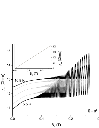
Figure 1: Dependencies of the dissipative resistivity of 2D electrons, $\displaystyle\rho_{xx}$, on perpendicular magnetic field taken at different temperatures: from bottom to top T=5.5, 6.9, 8.5, 10.1, and 10.9K. The inserts shows the Hall resistivity, $\displaystyle\rho_{xy}$, in a perpendicular magnetic field at the same set of temperatures as in the main plot. Angle $\displaystyle\theta=0^{0}$.

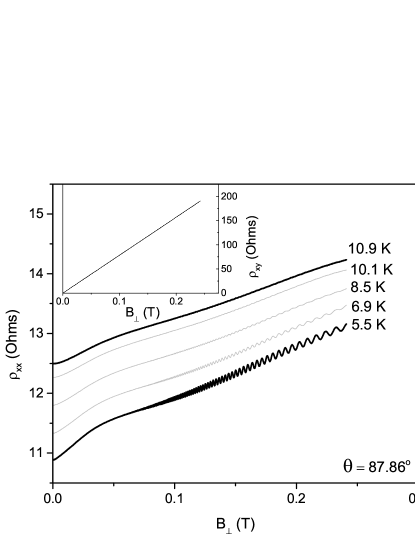
Figure 2: Dependencies of the dissipative resistivity of 2D electrons, $\displaystyle\rho_{xx}$, on perpendicular magnetic field taken at different temperatures: from bottom to top T=5.5, 6.9, 8.5, 10.1, and 10.9K. The inserts shows the Hall resistivity, $\displaystyle\rho_{xy}$, in a perpendicular magnetic field at the same set of temperatures as in the main plot. Angle $\displaystyle\theta=87.86^{0}$.

To facilitate the analysis of the oscillating content, the monotonic background $\displaystyle\rho^{b}_{xx}$, obtained by an averaging of the oscillations in reciprocal perpendicular magnetic fields, is removed from the magnetoresistivity $\displaystyle\rho_{xx}$($\displaystyle B_{\perp}$). Figure 3 presents the remaining oscillating content of the magnetoresistivistity, $\displaystyle\rho_{MISO}$, as a function of the reciprocal perpendicular magnetic field $\displaystyle B^{-1}_{\perp}$ for two temperatures as labeled. The thin solid lines indicate envelopes of the oscillating content used in the analysis below.

For disentangled subbands Figure 3(a) demonstrates that at the high temperature $\displaystyle T$=10.9 K the MISO magnitude is smaller than the one at $\displaystyle T$=5.5 K. An analysis of the MISO envelope indicates that the MISO magnitude decreases exponentially with $\displaystyle 1/B_{\perp}$ at a small $\displaystyle 1/B_{\perp}$. The rate of the exponential decrease is stronger at the higher temperature. Both the thermal suppression of MISO and the enhancement of the MISO reduction with $\displaystyle 1/B_{\perp}$ result from the increase of the quantum scattering rate of 2D electrons, $\displaystyle 1/\tau_{q}$, due to the increase of electron-electron scattering at high temperatures.

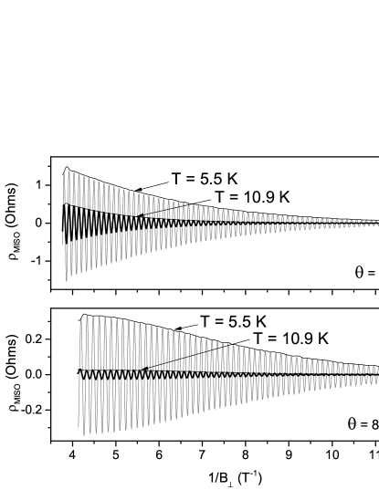
Figure 3: Oscillating content of magnetoresitivity $\displaystyle\rho_{xx}$ at two different temperatures as labeled. (a) disentangled subbands at angle $\displaystyle\theta=0^{0}$; (b) entangled subbands at angle $\displaystyle\theta=87.05^{0}$.

Figure 3(b) demonstrates the dependence of MISO on $\displaystyle 1/B_{\perp}$ for the magnetically entangled subbands at $\displaystyle\theta=$ 87.05 degrees. The decrease of MISO magnitude with $\displaystyle 1/B_{\perp}$ is different from the exponential decrease of the disentangled subbands. The magnetic field dependence tends to saturate at small $\displaystyle 1/B_{\perp}$ in contrast to the one shown in Figure 3(a). For the entangled subbands the MISO magnitude is significantly reduced. Furthermore a rough analysis indicates that the relative decrease of the MISO magnitude with the temperature is substantially stronger than the one for disentangled subbands. In particular, at $\displaystyle 1/B_{\perp}=$ 5 (1/T) for the disentangled subbands the ratio between MISO magnitudes at $\displaystyle T_{1}$=5.5K and $\displaystyle T_{2}$=10.9 K is close to 3, while for the entangled subbands the ratio is larger and close to 10.

Figure 4 presents an evolution of the temperature dependence of the MISO magnitude with the angle $\displaystyle\theta$ at fixed $\displaystyle B_{\perp}$=5 (1/T). Figure 4(a) shows the dependence of the normalized MISO magnitude on $\displaystyle T^{2}$. At a small subbands entanglement ($\displaystyle\theta=0^{0}$ and $\displaystyle 84.59^{0}$) the MISO magntitude drops exponentially with $\displaystyle T^{2}$ in a good agreement with the solid straight line presenting the $\displaystyle T^{2}$ exponential decrease at $\displaystyle\theta=0^{0}$. At larger angles ($\displaystyle\theta=87.05^{0}$ and $\displaystyle 87.86^{0}$) the MISO drop becomes stronger and deviates from the $\displaystyle T^{2}$ dependence.

In Figure 4(b) the symbols present the dependence of normalized MISO amplitude on temperature $\displaystyle T$. The solid straight lines demonstrate the exponential decrease with $\displaystyle T$. At small subbands entanglement ($\displaystyle\theta$=0; 84.59 degrees) the MISO magntitude does not decrease exponentially with $\displaystyle T$. The dependence deviates considerably from the solid straight line. In contrast at the largest angle (87.86 degrees) the MISO reduction is consistent with the exponential decrease with $\displaystyle T$ and follows the solid straight line. Thus, Figure 4 shows that the decrease of MISO amplitude with temperature is qualitatively different for the entangled subbands, indicating a new mechanism leading to the MISO damping. This new regime of thermal MISO damping is analyzed below within a model, taking into account the magnetic entanglement of 2D subbands.

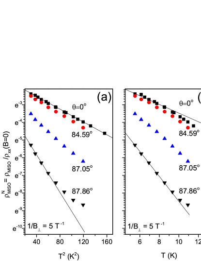
Figure 4: Temperature dependence of normalized amplitude of MISO, $\displaystyle\rho^{N}_{MISO}=\rho_{MISO}/\rho_{xx}({\bf B}=0)$ at $\displaystyle B^{-1}_{\perp}$ = 5 (1/T). (a) The dependence is plotted vs $\displaystyle T^{2}$; (b) the dependence is plotted vs $\displaystyle T$.

IV Model of Quantum Electron Transport

In perpendicular magnetic fields (at $\displaystyle\theta=$0^o) a microscopic theory of MISO is presented in papers Ref.[^{13; 14; 15}]. In this theory the electron spectra of two subbands evolve in magnetic fields quite independently. The reason is that at $\displaystyle\theta=$0^o the lateral (in the 2D layer) and vertical (perpendicular to the layer) electron motions are separable and do not affect each other. In a tilted magnetic field there is a component of the field, $\displaystyle B_{\parallel}$, which is parallel to the 2D conducting layer. This parallel component couples the lateral and vertical electron motions and electron spectra of two subbands become to be magnetically entangled. A MISO model, which takes into account this magnetic entanglement between two subbands, is proposed recently. The model demonstrates significant decrease of MISO amplitude with the magnetic field tilt. ¹⁶ A comparison with corresponding experiments indicates that the magnetic entanglement between subbands is the dominant mechanism leading to the angular decrease of the MISO amplitude in GaAs quantum wells. Zeeman spin splitting is found to provide a sub-leading contribution to the effect. ¹⁶

Below this model is used to analyze the temperature dependence of the MISO amplitude in tilted magnetic fields. The Zeeman effect is ignored. The analysis reveals an $\displaystyle universal$ temperature dependent factor, which controls the MISO amplitude in magnetically entangled subbands. The amplitude reduction is found to be exponential with the temperature in the regime of a strong magnetic entanglement. In many respects the physics of this additional temperature factor is similar to the one for SdH oscillations. The obtained factor describes general MISO property.

IV.1 Spectrum in tilted magnetic field

Let 2D electrons propagate along $\displaystyle xy$-plane and the $\displaystyle z$-axes is perpendicular to the plane. In quantum wells the spatial subbands are the result of quantization of the electron wave function in the $\displaystyle z$-direction. Index $\displaystyle i$=1(2) labels the low (high) subband with the energy $\displaystyle E_{1}$($\displaystyle E_{2}$) at the bottom of the subband. The subband separation is $\displaystyle\Delta_{12}=E_{2}-E_{1}$.

With no in-plane magnetic field applied the spatial subbands are coupled to each other via elastic scattering. An in-plane magnetic field, $\displaystyle B_{\parallel}$, provides an additional coupling via Lorentz force coming from the last term of the Hamiltonian $\displaystyle H$ presented by Eq.(2). This additional $\displaystyle B_{\parallel}$-coupling preserves the degeneracy of the quantum levels but induces variations of the electron spectrum, which, due to the relativistic origin of the Lorentz force, are dependent on the energy (velocity). These spectrum variations destroy the complete spectral overlap between Landau levels from different subbands, existing at zero in-plane magnetic field. This leads to the angular decrease of the MISO amplitude. ¹⁶ Below we investigate how this decrease depends on the temperature following to the developed approach.¹⁶

To estimate the effect the electron spectrum of an ideal two subband system without impurity scattering is computed numerically in a titled magnetic field. The impurity scattering is introduced then by a broadening of the bare quantum levels using Gaussian shape of the DOS with the preserved level degeneracy.

We consider a quantum well of a width $\displaystyle d$ in $\displaystyle z$-direction formed by a rectangular electrostatic potential $\displaystyle V(z)$ with infinitely high walls and placed in a titled magnetic field $\displaystyle{\bf B}=(-B_{\parallel},0,B_{\perp})$. Electrons are described by the Hamiltonian¹⁶:

$$H=\frac{\hbar^{2}k_{x}^{2}}{2m_{0}}+\frac{e^{2}B_{\perp}^{2}}{2m_{0}}x^{2}+\frac{\hbar^{2}k_{z}^{2}}{2m_{0}}+V(z)+\frac{e^{2}B_{\parallel}^{2}}{2m_{0}}z^{2}+\frac{e^{2}B_{\perp}B_{\parallel}}{m_{0}}xz,\\$$ (2)

where $\displaystyle m_{0}$ is electron band mass. To obtain Eq.(2) we have used the gauge (0,$\displaystyle B_{\perp}x+B_{\parallel}z$,0) of the vector potential and applied the transformation $\displaystyle x\rightarrow x-\hbar k_{y}/eB_{\perp}$.

The first four terms of the Hamiltonian describe the 2D electron system in a perpendicular magnetic field. The corresponding eigenfunctions of the system are $\displaystyle|N,\xi\rangle$, where $\displaystyle N$=0,1,2.. presents $\displaystyle N$-$\displaystyle th$ Landau level (the lateral quantization) and $\displaystyle\xi=S,AS$ describes the symmetric (S) and antisymmetric (AS) configurations of the wave function in the $\displaystyle z$-direction (vertical quantization): $\displaystyle|N,S\rangle=|N\rangle(2/d)^{1/2}\cos(\pi z/d)$ and $\displaystyle|N,AS\rangle=|N\rangle(2/d)^{1/2}\sin(2\pi z/d)$.

Using functions $\displaystyle|N,\xi\rangle$ as the basis set , one can present the Hamiltonian in matrix form. The matrix contains four matrix blocks: $\displaystyle\hat{H}=(\hat{E}^{S},\hat{T};\hat{T},\hat{E}^{AS})$, where the semicolon separates rows.The diagonal matrices, $\displaystyle\hat{E}^{S}$ and $\displaystyle\hat{E}^{AS}$, represent energy of the symmetric and antisymmetric wave functions in different orbital states $\displaystyle N$:

$$\begin{split}&E^{S}_{mn}=\delta_{mn}[\hbar\omega_{c}((n-1)+\frac{1}{2})+\frac{e^{2}B_{\parallel}^{2}d^{2}[\frac{1}{12}-\frac{1}{2\pi^{2}}]}{2m_{0}}]\\ &E^{AS}_{mn}=\delta_{mn}[\hbar\omega_{c}((n-1)+\frac{1}{2})+\Delta_{12}+\frac{e^{2}B_{\parallel}^{2}d^{2}[\frac{1}{12}-\frac{1}{8\pi^{2}}]}{2m_{0}}]\end{split}$$ (3)

where $\displaystyle\Delta_{12}=E_{2}-E_{1}$ is the energy difference between bottoms of two spatial subbands and indexes $\displaystyle m$=1,2…$\displaystyle N_{max}$ and $\displaystyle n$=1,2…$\displaystyle N_{max}$ numerate rows and columns of the matrix correspondingly. These indexes are related to the orbital number $\displaystyle N$: $\displaystyle n,m=N+1$, since the orbital number $\displaystyle N=0,1,2..$. In numerical computations the maximum number $\displaystyle N_{max}$ is chosen to be about twice larger than the orbital number $\displaystyle N_{F}$ corresponding to Fermi energy $\displaystyle\epsilon_{F}$. Further increase of $\displaystyle N_{max}$ shows a very small (within 1%) deviation from the dependencies obtained at $\displaystyle N_{max}\approx 2N_{F}$. This also indicates that the contributions of the third and higher spatial subbands with a higher energy can be ignored in the spectrum computation. It supports the two subband approximation used in the paper.

The first term in Eq.(3) describes the orbital quantization of electron motion. The last term in Eq.(3) describes diamagnetic shift of the quantum levels and relates to the fifth term in Eq.(2). In the basis set $\displaystyle|N,\xi\rangle$ the diamagnetic term is proportional to $\displaystyle\langle\xi|z^{2}|\xi\rangle$. The diamagnetic terms do not depend on $\displaystyle N$. The diamagnetic terms lead to an increase of the gap, $\displaystyle E_{g}$, between bottoms of subbands with the in-plane magnetic field:

$$E_{g}(B_{\parallel})=\Delta_{12}+\frac{3}{16\pi^{2}}\frac{e^{2}B_{\parallel}^{2}d^{2}}{m_{0}}$$ (4)

The off-diagonal matrix $\displaystyle\hat{T}$ is related to the last term in Eq.(2). This matrix mixes symmetric and antisymmetric states. Since $\displaystyle x=l_{B\perp}(a^{*}+a)/\sqrt{2}$ works as the raising $\displaystyle a^{*}$ and lowering $\displaystyle a$ operators of the Landau orbits, the last term in Eq.(2) couples Landau levels with orbital numbers different by one. Here $\displaystyle l_{B\perp}=(\hbar/eB_{\perp})^{1/2}$ is the magnetic length in $\displaystyle B_{\perp}$. As a result, for $\displaystyle n>m$ the matrix element $\displaystyle T_{mn}$ between states $\displaystyle|N,S\rangle$ and $\displaystyle|N+1,AS\rangle$ is

$$\begin{split}T_{mn}&=\delta_{m+1,n}\frac{e^{2}B_{\parallel}B_{\perp}l_{B\perp}}{m_{0}}\langle N|\frac{a^{*}+a}{\sqrt{2}}|N+1\rangle\langle S|z|AS\rangle\\ &=\delta_{m+1,n}\hbar\omega_{c}\Big{[}\frac{16B_{\parallel}d}{9\pi^{2}B_{\perp}l_{B\perp}}\Big{]}(n/2)^{1/2}\end{split}$$ (5)

The matrix $\displaystyle\hat{T}$ is a symmetric matrix: $\displaystyle T_{mn}=T_{nm}$.

The Hamiltonian $\displaystyle\hat{H}$ is diagonalized numerically at different magnetic fields $\displaystyle B_{\perp}$ and $\displaystyle B_{\parallel}$. To analyze the spectrum the obtained eigenvalues of the Hamiltonian are numerated in ascending order using positive integer index $\displaystyle l$=1,2…., which is named below as Landau level index.

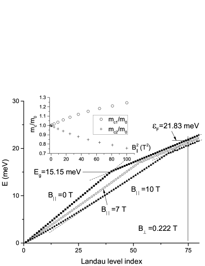
Figure 5: Dependence of the energy of Landau levels, counted from the bottom of the lowest subband in GaAs quantum well of width $\displaystyle d$=27 nm, on Landau level index, $\displaystyle l$, at different in-plane magnetic fields as labeled. Each symbol corresponds to a Landau level. Kinks in the dependencies occur at the energy corresponding to the bottom of the second subband, $\displaystyle E_{g}$. Decrease of the slope of the dependencies at $\displaystyle\epsilon<E_{g}$ with $\displaystyle B_{\parallel}$ indicates increase of the cyclotron mass $\displaystyle m_{c1}$ in the first subband. The independence of the slope on $\displaystyle B_{\parallel}$ at $\displaystyle\epsilon>E_{g}$ suggests decrease of the mass $\displaystyle m_{c2}$ in the second subband with $\displaystyle B_{\parallel}$. Vertical line at $\displaystyle l$=75 marks the last populated Landau level in the studied system. $\displaystyle B_{\perp}$=0.222T. Insert shows divergence of cyclotron masses in two subbands with the in-plane magnetic field.

Figure 5 presents a dependence of the Landau level energy, counted from the bottom of the first subband, on the index $\displaystyle l$ for different parallel magnetic fields as labeled. In the figure each symbol corresponds to a Landau level. At $\displaystyle B_{\parallel}$=0 T and $\displaystyle\epsilon<E_{g}=\Delta_{12}$ the quantum levels correspond to the first subband. These levels are evenly separated by the cyclotron energy $\displaystyle\Delta_{c}=\hbar\omega_{c}$, forming a straight line. The slope of this line is inversely proportional to the electron mass, $\displaystyle m_{0}$, since $\displaystyle\Delta_{c}\sim 1/m_{0}$. The slope is also inversely proportional to the density of states (DOS) since DOS $\displaystyle\sim m_{0}$ for 2D parabolic bands. At $\displaystyle\epsilon>E_{g}$ the slope of the straight line is abruptly reduced by factor two. This results from the contribution of the second subband to the total density of states, which starts at $\displaystyle\epsilon>E_{g}$. Since the mass in the second subband, $\displaystyle m_{0}$, is the same the total DOS is doubled and the slope is reduced by factor two. The transition between these two straight lines occurs at $\displaystyle\epsilon=E_{g}$ and corresponds to the energy of the bottom of the second subband $\displaystyle E_{2}$.

At $\displaystyle B_{\parallel}$=7 T and $\displaystyle\epsilon<\Delta_{12}$ the electron spectrum is different. At the same index $\displaystyle l$ the Landau levels of the first subband have a lower energy indicating an $\displaystyle increase$ of the cyclotron mass in the subband: $\displaystyle m_{c1}>m_{0}$. This is the effect of the entanglement between subbands, induced by the in-plane magnetic field: the eigenstate $\displaystyle\Psi_{l}$ of electron performing a cyclotron motion in the tilted magnetic field is now a linear superposition of the symmetric $\displaystyle|N,S\rangle$ and antisymmetric states $\displaystyle|N+n,AS\rangle$ of the Hamiltonian (Eq.(2)) at $\displaystyle B_{\parallel}$=0T. Although at $\displaystyle B_{\parallel}$=7 T the open symbols form apparent straight line, an analysis indicates deviations of the data from the linear dependence revealing a non-parabolicity of the spectrum. To simplify the presentation we neglect these deviations and approximate the spectrum by a straight line. In other words we consider the spectrum to be parabolic. Similar to the spectrum at $\displaystyle B_{\parallel}$=0T the straight line changes its slope due to the contribution of the second subband to the DOS. The slope change occurs at a higher energy, $\displaystyle E_{g}$: $\displaystyle E_{g}>\Delta_{12}$ due to contribution of the diamagnetic terms to the gap (see Eq.(4)). Within accuracy of one percent the changed slope coincides with the slope obtained at $\displaystyle B_{\parallel}$=0T at $\displaystyle\epsilon>\Delta_{12}$. This indicates that at $\displaystyle\epsilon>E_{g}$ the total density of states is preserved and, therefore, the effective mass in the second subband is reduced by the in-plane field $\displaystyle B_{\parallel}$: $\displaystyle m_{c2}<m_{0}$, since $\displaystyle m_{c1}+m_{c2}=2m_{0}\sim$ total DOS at high energies. Progressively stronger variations of the masses are seen at higher in-plane field $\displaystyle B_{\parallel}$=10T.

The insert to the figure shows relative variations of the cyclotron masses in the two subbands induced by the in-plane magnetic field. The insert demonstrates that at small in-plane magnetic fields the mass divergence is proportional to the square of the field. An analysis of the two subband model in a small in-plane magnetic field, given in Appendix A, provides further support to the presented interpretation of the electron spectra.

The insert in Figure 2 presents the Hall resistance taken at large tilt: $\displaystyle\theta=86.87$ degrees. The data indicates that the Hall coefficient, $\displaystyle R_{H}=1/en_{T}$, which is the slope of the shown line, does not depend on the in-plane magnetic field. This suggests that the total density $\displaystyle n_{T}=n_{1}+n_{2}$ and, thus, the electron population of Landau levels at fixed $\displaystyle B_{\perp}$: $\displaystyle l_{p}\approx n_{T}/n_{0}$ do not depend on $\displaystyle B_{\parallel}$. Here $\displaystyle n_{0}=eB_{\perp}/(\pi\hbar)$ is the degeneracy of Landau level (including the spin degeneracy) and $\displaystyle l_{p}$ is the index of the highest populated level. In Figure 5 the vertical line at $\displaystyle l$=75 marks the highest populated Landau level at $\displaystyle B_{\perp}$=0.222 T in the studied sample. At a fixed electron density (electron population) the increase of the electron mass $\displaystyle m_{c1}$ drives the Fermi energy, $\displaystyle E_{F}$, down, while the increase of the energy gap $\displaystyle E_{g}$ between the subbands moves the Fermi energy up. An interplay between these two effects results in a weak decrease of the Fermi energy with the in-plane magnetic field in the studied system.

The presented analysis above indicates that in tilted magnetic fields the cyclotron masses in two subbands are different: $\displaystyle m_{c1}>m_{c2}$. Different cyclotron masses lead to different frequencies of the DOS oscillations, induced by the orbital quantization in the energy space. Namely, in the first subband the DOS $\displaystyle\nu_{1}(\epsilon)$ oscillates at frequency $\displaystyle f_{1}=1/\hbar\omega_{c1}\sim m_{c1}$, while in the second subband the DOS, $\displaystyle\nu_{2}(\epsilon)$ oscillates at frequency $\displaystyle f_{2}=1/\hbar\omega_{c2}\sim m_{c2}$, where $\displaystyle\omega_{ci}$ is the cyclotron frequency in $\displaystyle i$-th subband. Thus at the same $\displaystyle B_{\perp}$ the frequency $\displaystyle f_{1}$ is higher than $\displaystyle f_{2}$ since $\displaystyle m_{c1}>m_{c2}$. The difference between frequencies results in a beating of the total DOS oscillations in the energy space as shown in Figure 6.

Figure 6: Energy dependence of the normalized density of states in the vicinity of Fermi energy: $\displaystyle\delta\epsilon=\epsilon-\epsilon_{F}$ in quantum well of width $\displaystyle d$=33 nm with two populated subbands, placed in perpendicular magnetic field $\displaystyle B_{\perp}$=0.244 T and in-plane magnetic fields $\displaystyle B_{\parallel}$ as labeled. At $\displaystyle B_{\parallel}>$0 the dependencies, shifted up for clarity, demonstrate beating pattern. The beating is related to the cyclotron mass divergence presented in the insert to Figure 5. Quantum scattering time $\displaystyle\tau_{q}^{(1)}=\tau_{q}^{(2)}=4ps$.

Figure 6 demonstrates the total DOS in a vicinity of Fermi energy: $\displaystyle\delta\epsilon=\epsilon-\epsilon_{F}$ at fixed perpendicular magnetic field $\displaystyle B_{\perp}$=0.244 T and different in-plane magnetic field $\displaystyle B_{\parallel}$ as labeled. The DOS is evaluated via numerical diagonalization of Hamiltonian (2) and consecutive broadening of the Landau levels. To demonstrate the DOS beating clearly we use the same quantum scattering time for both subbands $\displaystyle\tau_{q}^{(1)}=\tau_{q}^{(2)}$=4 ps. The obtained DOS oscillations are well described by an interference of two cosine functions. At $\displaystyle B_{\parallel}$=0T the DOS oscillations are significantly suppressed. This suppression is due to a destructive interference of the DOS oscillations in two subbands oscillating in anti-phase. This $\displaystyle\pi$-phase shift between the DOS oscillations leads to a MISO minimum, while two in-phase DOS oscillations should interfere constructively and lead to a MISO maximum (not shown). A noticeable property of the pattern is that the destructive interference at $\displaystyle B_{\parallel}$=0T does not depend on the energy. This property is tightly related to the fact that the DOS oscillates at the same frequency $\displaystyle f=1/\hbar\omega_{c}$ in both subbands at $\displaystyle B_{\parallel}$=0T.

The DOS oscillations at $\displaystyle B_{\parallel}$=0.66 T present an example of a partially constructive interference. A noticeable property of these oscillations is an increase of the amplitude of the oscillations with the energy. This property is due to the fact that, in contrast to the DOS interference at $\displaystyle B_{\parallel}$=0T, the frequencies of two DOS oscillations at $\displaystyle B_{\parallel}$=0.66 T are different: $\displaystyle f_{1}>f_{2}$. Thus, the interference pattern between these oscillations depends on the energy, exhibiting the beating. The DOS oscillations at $\displaystyle B_{\parallel}$=2.29, 2.75 and 3.45 T demonstrate the beating pattern with progressively shorter beating periods. The decrease of the beating period or increase of the beating frequency, $\displaystyle f_{b}$, is related to the increase of the difference frequency $\displaystyle\delta f=f_{1}-f_{2}=2f_{b}$ with $\displaystyle B_{\parallel}$. This increase is due to the mass divergence, shown in the insert to Figure 5, since $\displaystyle f_{i}\sim m_{i}$.

Below we explain qualitatively why the DOS beating leads to a temperature damping of MISO. More detailed consideration is given in the next section. The electron conductivity is determined by electrons in the $\displaystyle kT$ vicinity of the Fermi energy $\displaystyle\epsilon_{F}$.² The MISO amplitude is determined by the square of the amplitude of the DOS oscillations averaged within the $\displaystyle kT$ interval ^{13; 15}. Let’s assume that the energy interval $\displaystyle kT$ is much less than the beating period ($\displaystyle\sim 1/\delta f$): $\displaystyle kT\delta f\ll 1$. At this condition the MISO minimum (maximum) occurs when a node (anti-node) of the beating pattern is located in the $\displaystyle kT$ vicinity of $\displaystyle\epsilon_{F}$, since at the node (antinode) the DOS oscillations have a small (large) magnitude. At large temperatures $\displaystyle kT\delta f\gg 1$ the $\displaystyle kT$ interval contains both node (s) and antinode (s) and the averaged square of the DOS oscillations does not depend on the particular location of the beating pattern with respect to $\displaystyle\epsilon_{F}$. At this condition MISO oscillations should be suppressed. This consideration advocates for a decrease of the MISO amplitude with the temperature in magnetically entangled subbands.

IV.2 Temperature damping of MISO in magnetically entangled subbands

We consider 2D electron system with two populated parabolic subbands placed in a small quantizing perpendicular magnetic field $\displaystyle B_{\perp}$ and an in-plane magnetic field $\displaystyle B_{\parallel}$: $\displaystyle{\bf B}=(B_{\perp},B_{\parallel})$. In accordance with the presented numerical analysis of the electron spectrum (see also Appendix A) at a non-zero $\displaystyle B_{\parallel}$ the cyclotron masses, $\displaystyle m_{c1}>m_{c2}$ and frequencies, $\displaystyle\omega_{c1}<\omega_{c2}$, are different. This difference leads to the density of states (DOS) oscillating at different frequencies, $\displaystyle f_{i}$, in different subbands: $\displaystyle f_{i}=1/\hbar\omega_{ci}$, where index $\displaystyle i$=1(2) corresponds to first (second) subband.

At a small quantizing magnetic fields $\displaystyle\omega_{ci}\tau_{q}<1$ the main contribution to MISO comes from the fundamental harmonics of DOS oscillations. The DOS of $\displaystyle i$-th spatial subband, $\displaystyle\nu_{i}(\epsilon)$, reads^{3; 20}:

$$\begin{split}&\frac{\nu_{1}(\epsilon\geq 0)}{\nu_{01}}=1-2\delta_{1}\cos(2\pi f_{1}\epsilon)\\ &\frac{\nu_{2}(\epsilon\geq\ E_{g})}{\nu_{02}}=1-2\delta_{2}\cos(2\pi f_{2}(\epsilon-E_{g}))\end{split}$$ (6)

where $\displaystyle\nu_{0i}$ represents DOS at zero perpendicular magnetic field, $\displaystyle\delta_{i}=exp(-\pi/\omega_{ci}\tau_{q}^{(i)})$ is Dingle factor and $\displaystyle\tau_{q}^{(i)}$ is the quantum scattering time in $\displaystyle i$-th subbands. The parameters $\displaystyle\nu_{0i}$ describe DOS in a $\displaystyle kT$ vicinity of the Fermi energy. Within the $\displaystyle kT$ interval the energy dependence of these parameters in a weakly non-parabolic spectrum of 2D electrons, induced by the in the in-plane magnetic field, is neglected.

The 2D conductivity $\displaystyle\sigma$ is obtained from the following relation:

$$\sigma({\bf B})=\int d\epsilon\sigma(\epsilon)\left(-\frac{\partial f_{T}}{\partial\epsilon}\right)=\langle\sigma(\epsilon)\rangle$$ (7)

The integral is an average of the conductivity $\displaystyle\sigma(\epsilon)$ taken essentially for energies $\displaystyle\epsilon$ inside the temperature interval $\displaystyle kT$ near Fermi energy, where $\displaystyle f_{T}(\epsilon)$ is the electron distribution function at a temperature $\displaystyle T$. ^{3; 2} The brackets represent this integral below. We consider the regime of high temperatures: $\displaystyle f_{i}kT\gg 1$. In this regime Shubnikov de Haas oscillations are suppressed but MISO survive.

The conductivity $\displaystyle\sigma(\epsilon)$ is proportional to square of the total density of states: $\displaystyle\sigma(\epsilon)\sim(\nu_{1}(\epsilon)+\nu_{2}(\epsilon))^{2}$.^{30; 20} This relation yields the following term leading to MISO at small quantizing magnetic fields^{13; 15}:

$$\sigma_{MISO}(\epsilon)=\sigma_{D}^{(12)}\tilde{\nu_{1}}(\epsilon)\tilde{\nu_{2}}(\epsilon)$$ (8)

where $\displaystyle\tilde{\nu_{i}}(\epsilon)=\nu_{i}(\epsilon)/\nu_{0i}$ are the normalized density of states in each spatial subband. The parameter $\displaystyle\sigma_{D}^{(12)}(B_{\perp})$ is Drude like conductivity, accounting for inter-subband scattering.^{13; 15}

A substitution of Eq.(8) and Eq.(6) into Eq.(7) yields the following expression for the MISO of conductivity:

$$\sigma_{MISO}({\bf B})=4\sigma_{D}^{(12)}\delta_{1}\delta_{2}\langle\cos(2\pi f_{1}\epsilon)\cos(2\pi f_{2}(\epsilon-E_{g}))\rangle$$ (9)

An energy integration (see details in Appendix B) yields the final result:

$$\sigma_{MISO}({\bf B})=2\sigma_{D}^{(12)}\delta_{1}\delta_{2}\frac{X}{\sinh(X)}\cos(2\pi f_{2}E_{g}+2\pi\delta f\epsilon_{F})$$ (10)

, where parameter $\displaystyle X=2\pi^{2}kT\delta f$ and $\displaystyle\delta f=f_{1}-f_{2}$.

The obtained expression reproduces the results for disentangled subbands at $\displaystyle B_{\parallel}$=0T.^{13; 15} Indeed at $\displaystyle B_{\parallel}$=0T the difference frequency $\displaystyle\delta f$=0 and the temperature damping factor $\displaystyle A_{MISO}(T)=X/\sinh(X)=1$. The MISO maxima correspond to the condition $\displaystyle f_{2}E_{g}=j$, where $\displaystyle j$ is a positive integer, which is equivalent to Eq.(1) since $\displaystyle f_{2}=f=1/\hbar\omega_{c}$ and $\displaystyle E_{g}=\Delta_{12}$ at $\displaystyle B_{\parallel}$=0T. Finally the MISO magnitude is proportional to the product of two Dingle factors $\displaystyle\delta_{1}$ and $\displaystyle\delta_{2}$.^{13; 15}

For entangled subbands $\displaystyle\delta f>$0 and the temperature damping factor $\displaystyle A_{MISO}(T)=X/\sinh(X)$ decreases the MISO amplitude. This temperature decrease becomes exponential for $\displaystyle X>$1 since $\displaystyle\sinh(X)\sim\exp(X)$ for $\displaystyle X>$1. The parameter $\displaystyle X$ is proportional to the temperature and the difference frequency $\displaystyle\delta f=f_{1}-f_{2}$. At small in-plane magnetic fields, $\displaystyle B_{\parallel}$, the difference frequency is proportional to $\displaystyle B_{\parallel}^{2}$. This is shown in the insert to Figure 5 since $\displaystyle\delta f=f(m_{c1}-m_{c2})/m_{0}$ and $\displaystyle(m_{c1}-m_{c2})/m_{0}\approx\chi B_{\parallel}^{2}$ at small $\displaystyle B_{\parallel}$, where $\displaystyle\chi$ is a constant . Thus at small in-plane magnetic fields the parameter $\displaystyle X=2\pi^{2}kTf\chi B_{\parallel}^{2}=[2\pi^{2}km_{0}/(e\hbar)]\chi\tan^{2}(\theta)TB_{\perp}$ is proportional to $\displaystyle T$ and $\displaystyle B_{\perp}$. At larger $\displaystyle B_{\parallel}$ the mass divergence becomes weaker than $\displaystyle B_{\parallel}^{2}$, indicating a presence of high order terms of $\displaystyle B_{\parallel}^{2}$. Within the order of $\displaystyle B_{\parallel}^{6}$ the parameter $\displaystyle X$ reads:

$$X=\frac{2\pi^{2}km_{0}}{e\hbar}\chi(1-\xi B_{\parallel}^{2}+\eta B_{\parallel}^{4})\tan^{2}(\theta)TB_{\perp}$$ (11)

where $\displaystyle\chi$, $\displaystyle\xi$ and $\displaystyle\eta$ are constants. In Appendix A the constants $\displaystyle\chi=1.12\cdot 10^{-5}[d(nm)]^{2}$ and $\displaystyle\xi=1.91\cdot 10^{-5}[d(nm)]^{2}$ are computed analytically for the magnetically entangled subbands. Below we use the relation (11) to compare experiments with the expression (10).

In many respects the MISO temperature damping factor $\displaystyle A_{MISO}(T)$ is similar the one for Shubnikov de Haas oscillations, $\displaystyle A_{SdH}(T)=X_{SdH}/\sinh(X_{SdH})$, where $\displaystyle X_{SdH}=2\pi^{2}kT/(\hbar\omega_{ci})$.¹ The main difference is that the factor $\displaystyle A_{MISO}$ depends on the difference frequency $\displaystyle\delta f$ whereas the $\displaystyle A_{SdH}$ depends on the frequency $\displaystyle f_{i}=1/\hbar\omega_{ci}$. For parabolic subbands with the same masses $\displaystyle\delta f$=0 and the MISO damping factor $\displaystyle A_{MISO}$=1 is irrelevant. The MISO damping factor is important for non-parabolic spectra or parabolic spectra with different cyclotron masses in two subbands.

V Temperature dependence of MISO in tilted magnetic field

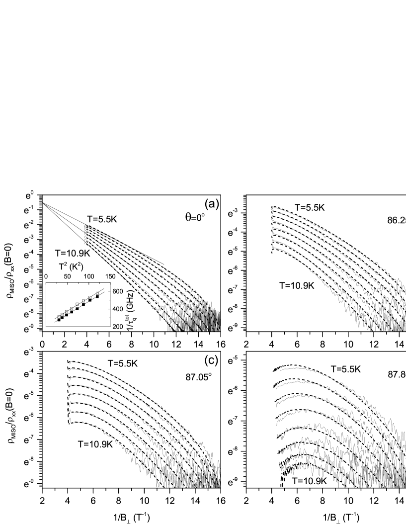
Figure 7: Dependence of normalized MISO amplitude $\displaystyle\rho_{MISO}/\rho_{xx}(0)$ on reciprocal magnetic field, $\displaystyle 1/B_{\perp}$, at different temperatures from top to bottom T=5.5, 6.14, 6.93, 7.74, 8.54, 9.34, 10.13 and 10.93K. and at angles as labeled. Solid lines represent experimental data. Dashed lines are numerical computations of MISO magnitude multiplied with normalizing function $\displaystyle F_{N}(B_{\perp})=0.55\cos(0.096/B_{\perp})$. (a) The numerical computations use quantum scattering times $\displaystyle\tau_{q}^{(1)}=\tau_{q}^{(2)}$ as fitting parameter to match with the experiment at different temperatures. In the insert, filled symbols present the obtained total quantum scattering rate: $\displaystyle 1/\tau_{q}^{tot}=2/\tau_{q}^{(1)}$. Open symbols present the rate determined from slopes of the thin straight lines shown in (a) ; (b)-(d) determined in (a) rates $\displaystyle 1/\tau_{q}^{tot}$ are used to compute MISO magnitude. The computed dependencies are shifted vertically to match with experiment, using normalizing factor $\displaystyle K(T)$. $\displaystyle d=26$nm. Sample S1.

In this section we compare the described model above and numerical computations of MISO with experiment. We start with the comparison between the numerical estimations and experiment.

Figure 7 presents dependence of MISO amplitude on reciprocal magnetic field, $\displaystyle 1/B_{\perp}$, measured at different temperatures between 5.5K and 10.9K. Panels (a)-(d) show the dependencies taken at different angles $\displaystyle\theta$ between the normal to 2D layer and the direction of the magnetic field $\displaystyle\bf B$. The dashed lines present results of numerical computations of MISO magnitude.

Figure 7(a) presents the dependencies taken at $\displaystyle\theta=0^{0}$. At this angle the entanglement between subbands is absent and $\displaystyle A_{MISO}=$1. The MISO magnitude decreases strongly with the reciprocal magnetic field, $\displaystyle 1/B_{\perp}$. This decrease is due to the exponential decrease of Dingle factors $\displaystyle\delta_{i}$ with $\displaystyle 1/B_{\perp}$: $\displaystyle\delta_{i}=exp(-\pi/\omega_{ci}\tau_{q}^{(i)})$. In accordance with Eq.(10), the MISO magnitude is proportional to the product of the Dingle factors. For disentangled subbands the cyclotron frequencies $\displaystyle\omega_{c1}$ and $\displaystyle\omega_{c2}$ are the same since $\displaystyle m_{c1}=m_{c2}=m_{0}$. Thus, the dependencies of the MISO amplitude on $\displaystyle 1/B_{\perp}$, plotted in semi-log scale, should be straight lines with the slope proportional to the sum of quantum scattering rates in two subbands: $\displaystyle 1/\tau_{q}^{(1)}+1/\tau_{q}^{(2)}$. In Figure 7(a) thin solid straight lines present the linear approximation of the measured dependencies. At higher temperature the slope of the lines becomes larger, indicating an increase of the quantum scattering rate with the temperature increase. In the insert to Figure 7(a) open symbols presents the temperature dependence of total quantum scattering rate $\displaystyle 1/\tau_{q}^{tot}=1/\tau_{q}^{(1)}+1/\tau_{q}^{(2)}$, extracted from these slopes.

A noticeable feature of the linear approximation is the convergence of the straight lines to the single point at $\displaystyle 1/B_{\perp}$=0T. This feature follows from Eq.(10) since $\displaystyle\delta_{1}\delta_{2}\rightarrow$1 and, thus, becomes temperature independent at $\displaystyle 1/B_{\perp}\rightarrow$0. Another noticeable feature is the apparent deviation of the measured dependencies from the straight lines at $\displaystyle 1/B_{\perp}>$10 (1/T). The origin of this deviation is under investigation and is not the focus of this study. We have found that a normalization of Eq.(10) by a temperature independent function $\displaystyle F_{N}(B_{\perp})$ leads to a good agreement between experiment and the model.

In Figure 7(a) the dashed lines present results of the numerical evaluation of the MISO magnitude. For each temperature the MISO magnitude is evaluated numerically with only one fitting parameter - the total quantum scattering rate $\displaystyle 1/\tau_{q}^{tot}$. The computed dependence is multiplied by the normalizing function $\displaystyle F_{N}(B_{\perp})=0.55\cos(0.096/B_{\perp})$, which bends down the linear dependence at $\displaystyle 1/B_{\perp}>$10 providing good agreement with the experiment. Obtained via this procedure the total scattering rate is shown by filled symbols in the insert to the figure. This scattering rate is found to be slightly lower than the one obtained via the first procedure (open symbols). Both dependencies demonstrate essentially the same variations of the quantum scattering rate with the temperature: $\displaystyle\delta(1/\tau_{q}^{tot})\sim T^{2}$, indicating the dominant contribution of the electron-electron scattering to the quantum electron lifetime.^{8; 9; 19}

For entangled subbands the cyclotron frequencies $\displaystyle\omega_{c1}$ and $\displaystyle\omega_{c2}$ are different since $\displaystyle m_{c1}>m_{c2}$. The difference leads to variations of the product of Dingle factors with the in-plane magnetic field in Eq.(10). Both numerical and analytical investigations of these variations demonstrates weak (within few percents ) corrections to MISO magnitude in the studied range of parameters. At $\displaystyle\tau_{q}^{(1)}=\tau_{q}^{(2)}$ these corrections are absent. Below we neglect these corrections and use $\displaystyle\tau_{q}^{(1)}=\tau_{q}^{(2)}$.

Figure 7(b) presents the magnetic field dependence of the MISO magnitude at $\displaystyle\theta=86.25^{0}$. At this angle the magnetic entanglement between two subbands leads to modifications of the MISO magnitude. Indeed at $\displaystyle 1/B_{\perp}\approx$5 (1/T) and $\displaystyle T$=5.5K the relative MISO magnitude is 0.058, which is considerably smaller the one shown in panel (a) - 0.094. At higher temperature T=10.9K the ratio between these two magnitudes becomes even smaller: 0.37. The numerical evaluations demonstrate the decrease of the MISO magnitude with the magnetic field tilt and the temperature and mostly capture the changes in the dependence shape. To better compare variations of the shape of the dependencies the overall magnitude of the numerical MISO is multiplied by factor $\displaystyle K(T)$, which is shown in the insert to Fig. 9. In Fig.7(b)-(d) the factor $\displaystyle K$ moves the computed dependencies vertically providing a better overlap with the experiment.

Figures 7(c) and (d) present the magnetic field dependence of the MISO magnitude at $\displaystyle\theta=87.05^{0}$ and $\displaystyle\theta=87.86^{0}$. At larger tilts the entanglement between subbands becomes stronger leading to stronger suppression of the MISO magnitude. The numerical computations continue to demonstrate good correlations with the shape of the magnetic field dependencies at different temperatures. These dependencies are not only quantitatively but qualitatively different from the ones shown in panel (a) for the disentangled subbands. In particular the convergence of the responses at $\displaystyle 1/B_{\perp}\rightarrow$0, which is apparent in panel (a), disappears in panels (c) and (d). Another noticeable feature is a consistent increase of variations of the normalizing coefficient $\displaystyle K$ with the temperature and the tilt, which is shown in the insert to Fig. 9. This MISO property will be discussed later.

All numerical dependencies, shown in panels (b), (c) and (d), are obtained at fixed $\displaystyle d$=26 nm, providing the best agreement with the shapes of experimental dependencies. The quantum scattering rates are determined from the response of disentangled subbands shown in panel (a). Thus, in the panels (b)-(d) the only variable fitting parameter, is the normalizing factor $\displaystyle K$, which moves the dependencies vertically but does not change their shape. Thus, as for the functional dependence the presented in panels (b)-(d) comparison between experiment and the model uses only one fitting parameter - the width of the quantum well $\displaystyle d$. The obtained width $\displaystyle d$=26 nm coincides with the actual width of the studied 2D layer. Thus the presented model captures the variations of the shape of the dependency of MISO on $\displaystyle 1/B_{\perp}$.

Presented in Fig.7 comparison with the numerical MISO is done under assumptions that the quantum scattering rates $\displaystyle 1/\tau_{q}^{(i)}$ and the Drude like conductivity $\displaystyle\sigma_{D}^{(12)}$ do not vary with the entanglement between subbands. The obtained agreement supports these assumptions, which we follow below.

To reveal the temperature damping factor $\displaystyle A_{MISO}(X)=X/\sinh(X)$ we compare our experimental data with the analytical expression (10) containing this factor. There are other factors ($\displaystyle\delta_{i},\sigma^{(12)}_{D}$) entering the expression. The presented comparison above with the numerical MISO as well as analytical considerations indicate that the product of these factors vary very weakly with the entanglement between subbands. Below we neglect these variations. To remove effects of these factors in the comparison between Eq.(10) and experiment, we divide each dependence in panels (b)-(d) (entangled subbands) by the dependence from panel (a) (disentangled subbands) taken at the same temperature $\displaystyle T$. This ratio $\displaystyle R_{exp}=\rho_{MISO}(\theta)/\rho_{MISO}(0)$ is compared with the one obtained from Eq.(10). In accordance with Eq.(10) at $\displaystyle\tau_{q}^{(1)}=\tau_{q}^{(2)}$ the ratio of the MISO magnitudes $\displaystyle R_{mod}=X/\sinh(X)$ and depends only on the parameter $\displaystyle X$. Thus, plotted vs $\displaystyle X$, the ratio $\displaystyle R_{exp}(X)$ should follow $\displaystyle A_{MISO}(X)=X/\sinh(X)$. To facilitate the comparison at $\displaystyle X>$1 both ratios are divided by $\displaystyle X$, yielding $\displaystyle R_{mod}/X\approx 2\exp(-X)$ at $\displaystyle X>$1. At large X $\displaystyle\ln(R/X)$ vs $\displaystyle X$ is, thus, straight line with a unity slope intersecting $\displaystyle y$-axis at $\displaystyle y_{0}$=2.

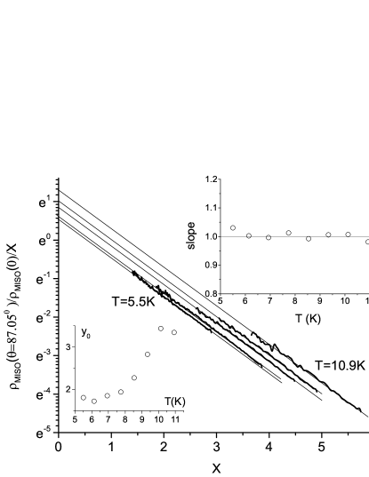
Figure 8: Dependence of ratio of MISO magnitude at $\displaystyle\theta=87.05^{0}$ to the one at $\displaystyle\theta=0^{0}$, normalized by $\displaystyle X$, on parameter $\displaystyle X$ at different temperatures $\displaystyle T$: 5.5, 7.74, 8.54, 9.34 and 10.9K. The parameter $\displaystyle X$ is computed from Eq.(11), using $\displaystyle\chi=1.12\cdot 10^{-5}[d(nm)]^{2}$, $\displaystyle\xi=1.91\cdot 10^{-5}[d(nm)]^{2}$, (see Appendix A), and $\displaystyle\eta=4\cdot 10^{-10}[d(nm)]^{4}$. Thin straight lines present linear dependencies with a unity slope, expected from Eq.(10). Upper insert presents temperature variations of slope magnitude, obtained from linear fit of the normalized ratio. Lower insert presents temperature evolution of the intersect $\displaystyle y_{0}$ of the linear fit with $\displaystyle y$-axis.

Figure 8 presents the dependence of the ratio $\displaystyle R_{exp}/X=\rho_{MISO}(\theta)/\rho_{MISO}(0)/X$ on the parameter $\displaystyle X$ for data at $\displaystyle\theta=87.05^{0}$. The parameter $\displaystyle X$ is evaluated from Eq.(11), using parameters $\displaystyle\chi=1.12\cdot 10^{-5}[d(nm)]^{2}$ and $\displaystyle\xi=1.91\cdot 10^{-5}[d(nm)]^{2}$, computed in Appendix A and parameter $\displaystyle\eta=\eta_{0}[d(nm)]^{4}$, where $\displaystyle\eta_{0}$ is a fitting parameter. At $\displaystyle d$=26 nm for all temperatures the experimental dependencies $\displaystyle\ln(R/X)$ vs $\displaystyle X$ follow the straight lines with unity slope. Some of the straight lines and the dependencies are shown in Figure 8 . The upper insert to Figure 8 demonstrates the magnitude of slopes obtained by a linear fit of the data. The slope magnitudes fluctuate around the expected value 1.

At $\displaystyle T$=5.5K the intersect of the corresponding straight line with y-axis yields $\displaystyle y_{0}\approx$1.72. This value is slightly below the expected value 2. With an increase of the temperature the intersect $\displaystyle y_{0}$ increases. The lower insert presents the increase of the intersect $\displaystyle y_{0}$ with the temperature obtained from the linear fit of the data. Thus, similar to the comparison with the numerical MISO, shown in Figure 7, the comparison in Figure 8 advocates for an additional factor $\displaystyle K^{*}(T,\theta)$ controlling the MISO magnitude.

At different temperatures and angles the normalizing factor $\displaystyle K^{*}$ is determined by the best overlap of experimental data with the expected dependence $\displaystyle 1/\sinh(X)$. To cancel effects related to this factor the experimental data $\displaystyle R_{exp}=\rho_{MISO}(\theta)/\rho_{MISO}(0)$ is divided by $\displaystyle K^{*}(T,\theta)$. This procedure leads to a collapse of experimental dependencies on the single curve $\displaystyle 1/\sinh(X)$, shown in Fig.9.

Figure 9 presents dependence of the normalized ratio $\displaystyle R^{*}=\rho_{MISO}(\theta)/\rho_{MISO}(0)/X/K^{*}$ on the parameter X for different temperatures and angles. The figure shows that for a broad range of temperatures and subband entanglement the normalized MISO magnitude, $\displaystyle R^{*}$, depends on the single parameter $\displaystyle X$, demonstrating good agreement with the modified MISO temperature damping factor $\displaystyle A_{MISO}/X=1/\sinh(X)$, shown by the dashed line in the figure. Thus, both comparisons, which are presented in Figure 7 and Figures 8 and 9, indicate that variations of MISO magnitude with the reciprocal magnetic field $\displaystyle 1/B_{\perp}$, temperature $\displaystyle T$, angles $\displaystyle\theta$ agree with the model and are controlled by MISO temperature damping factor $\displaystyle A_{MISO}=X/\sinh(X)$.

Both comparisons indicate also that there is another controlling factor $\displaystyle K^{*}(\theta,T)\approx K(\theta,T)$, which is beyond the presented model. The insert to Fig.9 shows temperature dependencies of normalizing coefficients $\displaystyle K$ (filled symbols) and $\displaystyle K^{*}$ (open symbols), obtained by different fitting procedures. Both procedures indicate the same temperature increase of both factors at a given angle. The data shows that the temperature variations of the parameters $\displaystyle K$ and $\displaystyle K^{*}$ are larger at larger $\displaystyle\theta$.

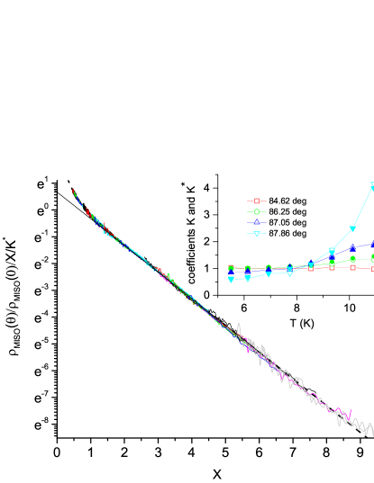
Figure 9: Dependence of the ratio $\displaystyle R$ of MISO magnitude obtained at angle $\displaystyle\theta$ to the one at $\displaystyle\theta$=0 deg normalized by $\displaystyle X$ and $\displaystyle K^{*}$: $\displaystyle R^{*}=R/X/K^{*}$ on parameter $\displaystyle X$ at different temperatures $\displaystyle T$: 5.5, 6.14, 6.93, 7.74, 8.54, 9.34, 10.13 and 10.9K and different angles $\displaystyle\theta$=84.62, 86.25, 87.05 and 87.86 deg (see text for detail). The parameter $\displaystyle X$ is computed from Eq.(11), using $\displaystyle\chi=1.12\cdot 10^{-5}[d(nm)]^{2}$, $\displaystyle\xi=1.91\cdot 10^{-5}[d(nm)]^{2}$, which are evaluated in Appendix A, and $\displaystyle\eta=4\cdot 10^{-10}[d(nm)]^{4}$ at $\displaystyle d$=26nm. Dashed line presents the dependence $\displaystyle 1/\sinh(X)$ expected from Eq.(10). Thin straight line presents the linear dependence $\displaystyle R/X$ vs $\displaystyle X$ with a unity slope and intersect $\displaystyle y_{0}$=2, expected from Eq.(10) at $\displaystyle X>$1. The insert presents temperature dependence of normalizing coefficients $\displaystyle K$(filled symbols) and $\displaystyle K^{*}$(open symbols) at different angles as labeled.

At large angles $\displaystyle\theta=87.05^{0}$ and $\displaystyle\theta=87.86^{0}$ the unity slope of the dependencies $\displaystyle R^{*}(X)$ is observed for all temperatures. However at smaller angles ($\displaystyle\theta=84.62^{0}$ and $\displaystyle\theta=86.25^{0}$) and high temperatures ($\displaystyle T>$9K) the dependencies $\displaystyle R^{*}(X)$ demonstrate slopes with magnitudes which are distinctly smaller than the unity. These dependencies are not shown in Fig.9. The presence of these deviations suggests a transitional function $\displaystyle F_{tr}(\delta f,\theta,T)$ between regimes of a weak and strong subband entanglement with a property $\displaystyle F_{tr}(\delta f,\theta,T)\rightarrow K^{*}(\theta,T)$ at a large $\displaystyle X$. The transitional function has not been investigated in this study. At large angles $\displaystyle\theta$ and temperatures (large $\displaystyle X$), where the normalizing coefficient $\displaystyle K^{*}$ and the function $\displaystyle F_{tr}(\delta f,\theta,T)$ are measurable, the access to small $\displaystyle X$ requires a very small $\displaystyle B_{\perp}$ (see Eq.(11). At this small $\displaystyle B_{\perp}$ the Dingle factors strongly suppress the MISO amplitude making the amplitude measurements not accurate. Measurements at smaller angles indicate the presence of the transitional function. However the magnitude of this function is small, making an analysis of the function to be not informative.

V.1 Effects of electron-electron interaction on MISO

Both Figure 8 and the insert to Figure 9 demonstrate an increase of the deviation between the experiment and model with the temperature increase. The increase of the deviation correlates with the increase of the temperature dependent contribution to the electron lifetime. Indeed the insert to Figure 7(a) shows that at $\displaystyle T$=10.9 K the contribution of electron-electron scattering to the quantum scattering rate is about 4 times larger than at $\displaystyle T$=5.5K and becomes dominant. This correlation suggests that effects of electron-electron interaction or Fermi-liquid effects may play important role leading to the deviation between Eq.(10) and experiment. Indeed, although ignored in the presented model, such effects are important for quantum oscillations, resulting in a renormalization of the electron mass and g-factor - the effects, which have been intensively investigated both theoretically and experimentally for several decades³.

Effects of the electron-electron interactions on the quantum scattering time, controlling the magnitude of quantum oscillations, are less frequently studied. Existing theory predicts that the amplitude of the fundamental harmonic of SdH oscillations is resilient to the temperature variations of the quantum scattering time, induced by the electron -electron interaction.^{31; 32} In other words the quantum scattering time, entering the Dingle factor for the fundamental harmonic of SdH oscillations, is a temperature independent parameter. This can be considered as a result of a modification of the electron lifetime by the electron-electron interaction. The modification leads to contributions, enhancing the SdH amplitude and compensating the temperature dependent part of the quantum scattering rate in the Dingle factor. In contrast the quantum scattering rate, entering the Dingle factor for the MISO amplitude, is temperature dependent property as shown in the insert to Figure 7(a).

To the best of our knowledge Fermi liquid effects related to MISO in magnetically entangled subbands have not been investigated. Assuming a similarity of the Fermi liquid contributions to the magnitude of SdH oscillations and MISO in entangled subbands, one should expect a relative increase of the MISO magnitude, which may explain the increase of the factors $\displaystyle K$ and $\displaystyle K^{*}$ with the temperature. The resilience of SdH amplitude to the electron-electron interactions can be obtained via an account of the interaction induced dependence of the electron-electron scattering rate on the energy $\displaystyle\epsilon$.³³ The electron-electron collision rate for an electron at energy $\displaystyle\epsilon$ counted from the Fermi energy $\displaystyle\epsilon_{F}$ is

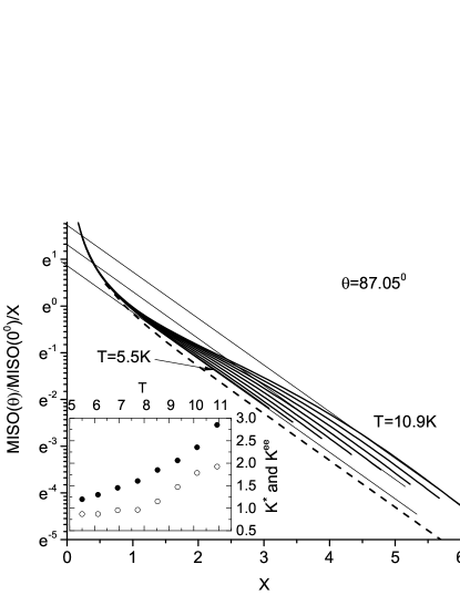
Figure 10: Dependence of ratio of MISO magnitude at $\displaystyle\theta=87.05^{0}$ to the one at $\displaystyle\theta=0^{0}$, normalized by $\displaystyle X$ on parameter $\displaystyle X$. The dependence is computed at $\displaystyle\epsilon_{F}^{*}=$8 meV and different temperatures from bottom to top $\displaystyle T$=5.5, 6.14, 6.93, 7.74, 8.54, 9.34, 10.13 and 10.9K using Eq.(14). The parameter $\displaystyle X$ is computed from Eq.(11), using $\displaystyle\chi=1.12\cdot 10^{-5}[d(nm)]^{2}$, $\displaystyle\xi=1.91\cdot 10^{-5}[d(nm)]^{2}$, obtained in Appendix A, and $\displaystyle\eta=4\cdot 10^{-10}[d(nm)]^{4}$. Thin straight lines present linear dependencies with a unity slope. Dashed line displays free electron response $\displaystyle 1/\sinh(X)$. The insert shows temperature evolution of factors $\displaystyle K^{*}$ and $\displaystyle K^{ee}$, characterizing maximal deviation of the experimental and model data from the free electron response.

$$\frac{1}{\tau_{ee}(\epsilon,T)}=\frac{\epsilon^{2}+\pi^{2}(kT)^{2}}{4\pi\hbar\epsilon_{F}}\ln\frac{q_{s}v_{F}}{\max(kT,\hbar\omega_{c}(\omega_{c}\tau_{tr})^{1/2})}$$ (12)

, where $\displaystyle v_{F}$ is Fermi velocity, $\displaystyle\tau_{tr}$ is transport scattering time and $\displaystyle q_{s}=2\pi e^{2}\nu$ is inversion screening length.^{30; 33}

The energy dependence of the electron scattering rate makes the Dingle factors $\displaystyle\delta_{i}$ to be energy dependent parameters:

$$\delta_{i}(\epsilon,T)=\exp\Big{(}-\frac{\tau_{im}^{-1}+\tau_{ee}^{-1}(\epsilon,T)}{\omega_{ci}/\pi}\Big{)}$$ (13)

, where $\displaystyle\tau_{im}$ is quantum scattering time due to impurity scattering. The time $\displaystyle\tau_{im}$ does not depend on the temperature while the electron-electron scattering time $\displaystyle\tau_{ee}$ is temperature dependent. The time $\displaystyle\tau_{ee}$ provides the $\displaystyle T^{2}$ contribution to the quantum scattering rate shown in the insert to Fig. 7(a) for the disentangled subbands.

The energy dependence of the Dingle factors $\displaystyle\delta_{i}$ is not accounted in the presented above analysis. The effect of the energy dependence of the $\displaystyle e-e$ scattering rate on the relative MISO magnitude: $\displaystyle\rho_{MISO}(\theta)/\rho_{MISO}(0^{0})=\sigma_{MISO}(\theta)/\sigma_{MISO}(0^{0})$ is evaluated below. Substitution of the relations (8), (6) and (13) into Eq.(7) leads to the following expression for the relative MISO magnitude:

$$\frac{\rho_{MISO}(\theta)}{\rho_{MISO}(0^{0})}=\frac{\langle\exp(-\epsilon^{2}/\epsilon_{0}^{2})\cos(2\pi\delta f\epsilon)\rangle}{\langle\exp(-\epsilon^{2}/\epsilon_{0}^{2})\rangle}$$ (14)

, where $\displaystyle\epsilon_{0}=(2\epsilon_{F}^{*}\hbar\omega_{c})^{1/2}$. In the estimation a possible difference in the $\displaystyle e-e$ scattering rate in two subbands and the temperature/magnetic field dependencies of the logarithmic factor in Eq.(12) are ignored. As a result in Eq.(14) the only fitting parameter is $\displaystyle\epsilon_{F}^{*}\sim\epsilon_{F}^{(i)}/\ln(q_{s}v_{F}^{(i)}/\max(kT,\hbar\omega_{c}(\omega_{c})^{1/2}$.

Figure 10 demonstrates the dependence of normalized relative MISO magnitude, $\displaystyle\rho_{MISO}(\theta)/\rho_{MISO}(0^{0})/X$ on parameter X obtained from Eq.(14) at angle $\displaystyle\theta$=87.05⁰, temperatures $\displaystyle T$= 5.5, 6.14, 6.93, 7.74, 8.54, 9.34, 10.13 and 10.9K and $\displaystyle\epsilon_{F}^{*}$=8 meV. The angle and temperatures corresponds to the experimental dependencies of the normalized relative MISO magnitude presented in Fig.8. In Fig.10 the dashed line shows the dependence $\displaystyle 1/\sinh(X)$ for free 2D electrons computed at $\displaystyle\epsilon_{0}\rightarrow\infty$. The obtained behavior suggests that the relative MISO magnitude can be presented as a product of $\displaystyle X/\sinh(X)$ and a finite function $\displaystyle F_{tr}(X,\theta,T)$:

$$\frac{\rho_{MISO}(\theta)}{\rho_{MISO}(0^{0})}=F_{tr}(X,\theta,T)\frac{X}{\sinh(X)}$$ (15)

Below we investigate properties of the function $\displaystyle F_{tr}(X,\theta,T)$. In Fig.10 at small $\displaystyle X<$1 the dependencies converge for all temperatures. This is related to the reduction of the difference frequency: $\displaystyle\delta f\rightarrow 0$ at $\displaystyle X\rightarrow 0$ since $\displaystyle\delta f$ is proportional to $\displaystyle X$. At $\displaystyle\delta f\rightarrow 0$ in Eq.(14) the cosine function tends to 1 and the ratio of the two integrals approaches unity. Thus at $\displaystyle X\rightarrow 0$ the function $\displaystyle F_{tr}(X,\theta,T)\rightarrow 1$ since $\displaystyle X/\sinh(X)\rightarrow 1$.

At large $\displaystyle X\rightarrow\infty$ but a finite temperature the function $\displaystyle F_{tr}(X,\theta,T)$ also tend to unity. To understand this property we note that in accordance with Eq.(11) a large $\displaystyle X$ corresponds to a large $\displaystyle B_{\perp}$ and, thus, to large $\displaystyle\hbar\omega_{c}$ and $\displaystyle\epsilon_{0}$. At $\displaystyle\epsilon_{0}\gg kT$ in Eq.(14) the Gaussian functions can be neglected that leads to the free electron result (10).

At an intermediate X the function $\displaystyle F_{tr}(X,\theta,T)$ deviates from unity and reaches a maximum. The increase of the function $\displaystyle F_{tr}(X,\theta,T)$ from the unity is a result of the electron-electron interaction and, thus, is a Fermi liquid effect. The electron-electron interaction leads to a decrease of the quantum lifetime of quasiparticles with the energy $\displaystyle\epsilon$ away from the Fermi energy.^{31; 32} Eq.(12) and Eq.(13) take into account this lifetime decrease and yields in Eq.(14) the Gaussian $\displaystyle\exp(-\epsilon^{2}/\epsilon_{0}^{2})$, which enhances the MISO amplitude. Mathematically the effect is due to a reduction of the range of the energy integration in Eq.(14) from $\displaystyle(-kT,kT)$, settled by the distribution function $\displaystyle f_{T}$ for free electrons, to a smaller range, which for the interacting electrons is additionally affected by the range narrowing factor $\displaystyle\exp(-\epsilon^{2}/\epsilon_{0}^{2})$. The energy averaging of the oscillating content ($\displaystyle\cos(2\pi\delta f\epsilon)$) in narrower energy interval leads to a suppression of the averaging and results in a larger value of the integral and, thus, the function $\displaystyle F_{tr}(X,\theta,T)$. ³³

In the experimentally studied range of parameters, the maximum of the function $\displaystyle F_{tr}(X,\theta,T)$ appears to be quite flat and can be approximated by a straight horizontal line, which acquires unity slope in Fig.10. This property agrees with the experiment. Three of these lines are shown in Fig.10. A coefficient $\displaystyle K^{ee}(T)\approx\max[F_{tr}(X,T)]$ characterizes the vertical displacement of these lines from the free electron response $\displaystyle 1/\sinh(X)$ (dashed line). Figure 10 demonstrates that the coefficient $\displaystyle K^{ee}(T)$ increases with the temperature. This behavior is also in agreement with the experiment shown in Fig.8.

The insert to Fig.10 demonstrates a comparison between coefficient $\displaystyle K^{*}$, obtained from experimental data presented in Fig.8 and coefficient $\displaystyle K^{ee}$, obtained from the model data presented in Fig.10. At $\displaystyle\epsilon_{F}^{*}$=8 meV both coefficients $\displaystyle K^{*}$, $\displaystyle K^{ee}$ and variations of these coefficients with the temperature are close to each other. Furthermore an evaluation of the temperature dependence of the quantum scattering rate, using the temperature dependent part of Eq.(12), yields $\displaystyle\tau_{q}^{-1}(T)-\tau_{q}^{-1}(0K)=\tau_{ee}^{-1}(\epsilon=0)=\pi(kT)^{2}/(4\hbar\epsilon_{F}^{*})\approx$1.2(GHz)$\displaystyle T^{2}$. This value is close to the inelastic scattering rate obtained in the experiment at $\displaystyle\theta$=0⁰ and shown in the insert to Fig.7(a): $\displaystyle\tau_{q}^{-1}(T)-\tau_{q}^{-1}(0K)\approx$1.5(GHz)$\displaystyle T^{2}$. Thus, the account of the electron-electron interaction improves the agreement between the experiment and model, revealing the interaction induced enhancement of MISO amplitude.

VI Summary

Magneto-intersubbands resistance oscillations (MISO) of highly mobile 2D electrons in symmetric GaAs quantum wells with two populated subbands are studied at different temperatures and at different angles $\displaystyle\theta$ between magnetic field $\displaystyle{\bf B}$ and the normal to 2D layer. The experiments indicate that the MISO magnitude decreases strongly with the temperature. For angles $\displaystyle\theta<80^{0}$ the MISO reduction is related to the increase of the quantum scattering rate due to the enhancement of electron-electron scattering at high temperatures. For angles $\displaystyle\theta>80^{0}$ new regime of strong MISO damping with the temperature is identified.

Proposed model considers the magnetic entanglement between subbands, which is induced by in-plane magnetic field, as the main reason of the new temperature damping. The entanglement changes the electron spectrum and leads to different cyclotron masses in two subbands. As a result the density of states exhibits beating with the difference frequency $\displaystyle\delta f$ proportional to the mass difference. The model yields universal temperature damping factor $\displaystyle A_{MISO}=X/\sinh(X)$, where $\displaystyle X=2\pi^{2}kT\delta f$.

A comparison of the model with the experiment demonstrates the presence of the factor $\displaystyle A_{MISO}$ but indicates an additional factor $\displaystyle K(T)$, which is beyond the free electron model. The factor $\displaystyle K$ leads to an effective enhancement of the MISO amplitude at high temperatures. An account of the electron-electron interaction explains the enhancement of the MISO amplitude and reveals the Fermi liquid origin of the factor K.

This work was supported by the National Science Foundation (Division of Material Research - 1702594) and by the Russian Foundation for Basic Research (project no. 20-02-00309).

VII Appendix A

In this section the spectrum of the entangled subbands is computed at $\displaystyle\theta$=90 deg. The cyclotron masses, $\displaystyle m_{ci}$ and difference frequency $\displaystyle\delta f\sim(m_{c1}-m_{c2})$, are evaluated then for the quasiclassical electron motion in a small $\displaystyle B_{\perp}$. The goal is estimation of the variations of the parameter $\displaystyle X\sim\delta f$ with the magnetic field $\displaystyle B_{\parallel}$ leading to Eq.(11).

At $\displaystyle B_{\perp}$=0 T ($\displaystyle{\bf B}=(-B_{\parallel},0,0)$) the Hamiltonian (2) is presented in the following form:

$$\begin{split}&H=\frac{\hbar^{2}k_{x}^{2}}{2m_{0}}+\frac{\hbar^{2}(k_{y}+\frac{eB_{\parallel}z}{\hbar})^{2}}{2m_{0}}+\frac{\hbar^{2}k_{z}^{2}}{2m_{0}}+V(z)=H_{0}+H_{1}\\ &H_{0}=\frac{\hbar^{2}}{2m_{0}}(k_{x}^{2}+k_{y}^{2}+k_{z}^{2})+V(z)\\ &H_{1}=\hbar\omega_{\parallel}k_{y}z+\frac{1}{2}m_{0}\omega_{\parallel}^{2}z^{2}\end{split}$$ (16)

,where $\displaystyle\omega_{\parallel}=eB_{\parallel}/m_{0}$ is the cyclotron frequency in in-plane magnetic field, $\displaystyle B_{\parallel}$. At $\displaystyle B_{\parallel}$=0T the corresponding eigenfunctions $\displaystyle|{\bf k},\xi\rangle$ of the system are plane waves, propagating in $\displaystyle x-y$ plane, and standing waves in $\displaystyle z$-direction , where wave vector $\displaystyle{\bf k}$ describes the lateral motion and $\displaystyle\xi=S,AS$ describes the symmetric (S) and antisymmetric (AS) configurations of the wave function in the $\displaystyle z$-direction (vertical quantization): $\displaystyle|{\bf k},S\rangle=|{\bf k}\rangle(2/d)^{1/2}\cos(\pi z/d)$ and $\displaystyle|{\bf k},AS\rangle=|{\bf k}\rangle(2/d)^{1/2}\sin(2\pi z/d)$.

Using functions $\displaystyle|{\bf k},\xi\rangle$ as the basis set , one can present the Hamiltonian as a 2$\displaystyle\times$2 matrix:

$$\begin{split}&H_{ij}=\epsilon_{i}^{0}\delta_{ij}+(1-\delta_{ij})h_{12}\\ &\epsilon_{i}^{0}=\frac{\hbar^{2}}{2m_{0}}(k_{x}^{2}+k_{y}^{2})+E_{i}+\frac{1}{2}m\omega_{\parallel}^{2}Z_{i}^{2}\\ &h_{12}=\hbar\omega_{\parallel}k_{y}Z_{0}\end{split}$$ (17)

, where $\displaystyle\delta_{ij}$ presents 2$\displaystyle\times$2 unit matrix, $\displaystyle Z_{0}=16d/(9\pi^{2})$, $\displaystyle Z_{1}^{2}=(1/12-1/(2\pi^{2}))d^{2}$ and $\displaystyle Z_{2}^{2}=(1/12-1/(8\pi^{2}))d^{2}$. Indexes $\displaystyle i,j$=1,2 describes first (1) and second (2) subbands. Energy $\displaystyle E_{i}$ corresponds to the bottom of $\displaystyle i$-th subband at $\displaystyle B_{\parallel}$=0T.

At $\displaystyle h_{12}\ll\epsilon_{2}^{0}-\epsilon_{1}^{0}$ diagonalization of the Hamiltonian $\displaystyle H_{ij}$ leads to the following spectrum:

$$\begin{split}&\epsilon_{i}({\bf k})\approx\epsilon_{i}^{0}({\bf k})\pm\frac{h_{12}^{2}}{\epsilon_{2}^{0}-\epsilon_{1}^{0}}(1-\frac{h_{12}^{2}}{(\epsilon_{2}^{0}-\epsilon_{1}^{0})^{2}})\approx\\ &\approx\epsilon_{i}^{0}({\bf k})\pm A\frac{\hbar^{2}k_{y}^{2}}{2m_{0}}\Big{(}1-\frac{A}{E_{g}}\frac{\hbar^{2}k_{y}^{2}}{2m_{0}}\Big{)}=\\ &=E_{i}+\frac{\hbar^{2}k_{x}^{2}}{2m_{xi}}+\frac{\hbar^{2}k_{y}^{2}}{2m_{yi}}\mp\gamma_{0}k_{y}^{4}\\ &A=\frac{2m_{0}Z_{0}^{2}}{E_{g}}\omega_{\parallel}^{2};E_{g}=\Delta_{12}+\frac{m_{0}(Z_{2}^{2}-Z_{1}^{2})}{2}\omega_{\parallel}^{2}\end{split}$$ (18)

, where lower (upper) sign corresponds to the first ($\displaystyle i$=1) (second (i=2)) subband, $\displaystyle\gamma_{0}=\hbar^{4}A^{2}/[(2m_{0})^{2}E_{g}]$ and $\displaystyle\Delta_{12}=E_{2}-E_{1}$. Eq.(18) indicates that due to the presence of the in-plane magnetic field the spectrum is anisotropic but still parabolic in the lowest order of $\displaystyle B_{\parallel}$ ($\displaystyle\sim B_{\parallel}^{2})$. The parameter $\displaystyle A$ controls the strength of the anisotropy leading to an increase (decrease) of the mass, $\displaystyle m_{y1}=m_{0}/(1-A)^{1/2}$ ($\displaystyle m_{y2}=m_{0}/(1+A)^{1/2}$) in $\displaystyle y$-direction for lower (upper) subband. In $\displaystyle x$-direction masses do not change: $\displaystyle m_{xi}=m_{0}$.

For a parabolic spectrum the cyclotron mass is $\displaystyle m_{c}=(m_{x}m_{y})^{1/2}$. ² To compute the cyclotron masses in the vicinity of Fermi energy $\displaystyle\epsilon_{F}$ for the non-parabolic spectrum we use the relation $\displaystyle m_{c}=(\hbar^{2}/2\pi)(\partial S/\partial\epsilon)$, where $\displaystyle S(\epsilon)$ is the area within the contour $\displaystyle\epsilon_{i}({\bf k})=\epsilon_{F}$.² For the spectrum (18) the result is

$$\begin{split}&m_{c1}=(m_{xi}m_{y1})^{1/2}\Big{(}1-\frac{3}{4}\frac{m_{y1}^{2}}{m_{0}^{2}}\frac{A^{2}}{E_{g}}\epsilon_{F1}\Big{)}\\ &m_{c2}=(m_{xi}m_{y2})^{1/2}\Big{(}1+\frac{3}{4}\frac{m_{y2}^{2}}{m_{0}^{2}}\frac{A^{2}}{E_{g}}\epsilon_{F2}\Big{)}\end{split}$$ (19)

, where $\displaystyle\epsilon_{Fi}$ is Fermi energy counted from the bottom of $\displaystyle i$-th subband. The result agrees with the numerical computation of the cyclotron masses presented in the insert to Fig.5: $\displaystyle m_{c1}$ ($\displaystyle m_{c2}$) increases (decreases) with the in-plane magnetic field. Furthermore the sum of the masses stays the same: $\displaystyle m_{c1}+m_{c2}=2m_{0}$ within the computed order $\displaystyle B_{\parallel}^{4}$.

Within the same order for difference frequency Eq.(19) yields:

$$\begin{split}&\delta f\approx f\Big{(}A-\frac{3}{4}\frac{\epsilon_{F1}+\epsilon_{F2}}{E_{g}}A^{2}\Big{)}\approx f\Big{[}\chi B_{\parallel}^{2}(1-\xi B_{\parallel}^{2})\Big{]};\\ &\chi=\frac{2e^{2}Z_{0}^{2}}{\Delta_{12}m_{0}};\xi=\frac{3}{4}\frac{\epsilon_{F1}^{0}+\epsilon_{F2}^{0}}{\Delta_{12}}\chi+\frac{1}{2}\frac{2e^{2}(Z_{2}^{2}-Z_{1}^{2})}{\Delta_{12}m_{0}}\end{split}$$ (20)

, where $\displaystyle\epsilon_{Fi}^{0}$ is Fermi energy counted form the bottom of $\displaystyle i$-th subband at zero magnetic field. For the studied system $\displaystyle\epsilon_{F1}^{0}$=21.83 (meV); $\displaystyle\epsilon_{F2}^{0}$=6.68 (meV) and $\displaystyle\Delta_{12}$=15.15(meV) yield $\displaystyle\chi=1.12\cdot 10^{-5}[d(nm]^{2}$ and $\displaystyle\xi=1.91\cdot 10^{-5}[d(nm]^{2}$. These results are used to compute the parameter $\displaystyle X$ in Eq.(11) up to terms proportional to $\displaystyle B_{\parallel}^{4}$.

VIII Appendix B

The expression (9) contains energy integration of a product of two cosine functions. To perform the integration we represent this product as a sum of two cosines, oscillating at frequency $\displaystyle f_{1}+f_{2}$ and $\displaystyle\delta f=f_{1}-f_{2}$. An integration of the cosine, oscillating at frequency $\displaystyle f_{1}+f_{2}$, leads to an exponentially small term $\displaystyle\sim\exp(-2\pi^{2}(f_{1}+f_{2})kT)$. Since $\displaystyle f_{i}kT\gg 1$ this term is neglected.

To perform the integration in the $\displaystyle kT$ vicinity of Fermi energy $\displaystyle\epsilon_{F}$ we substitute $\displaystyle\epsilon=u+\epsilon_{F}$. After the substitution the phase of the second cosine, oscillating at frequency $\displaystyle\delta f$ is a sum of two terms: $\displaystyle\alpha=\pi\delta fu\sim u$ and $\displaystyle\beta=2\pi(f_{2}\Delta_{g}+\delta f\epsilon_{F})$=const. The cosine can be rewritten, using the identity: $\displaystyle\cos(\alpha+\beta)=\cos(\alpha)\cos(\beta)-\sin(\alpha)\sin(\beta)$. An integration of the product of two sine functions in the vicinity of the Fermi energy yields zero, since $\displaystyle\sin(\alpha)$ is odd function of variable $\displaystyle u$, whereas $\displaystyle\partial f_{T}(u)/\partial u$ is even function of $\displaystyle u$. In result the integral is proportional to $\displaystyle\langle\cos(2\pi\delta fu)\rangle\cos(2\pi f_{2}\Delta_{g}+2\pi\delta f\epsilon_{F})$. The integration vs $\displaystyle u$ yields: $\displaystyle\langle\cos(2\pi\delta fu)\rangle=X/\sinh(X)$, where $\displaystyle X=2\pi^{2}kT\delta f$,² leading to Eq.(10).

References

- (1) D. Shoenberg Magnetic oscillations in metals, (Cambridge University Press, New York, 1984).
- (2) J. M. Ziman Principles of the theory of solids, (Cambridge at the University Press, 1972).
- (3) T. Ando, A. B. Fowler, and F. Stern, Rev. of Mod. Phys. B 54, 437 (1982).
- (4) Sankar D. Sarma, Aron Pinczuk Perspectives in Quantum Hall Effects, (Wiley-VCH, Weinheim, 2004).
- (5) P. T. Coleridge, Semicond. Sci. Technol. 5, 961 (1990).
- (6) D. R. Leadley, R. Fletcher, R. J. Nicholas, F. Tao, C. T. Foxon, and J. J. Harris, Phys. Rev. B 46, 12439 (1992).
- (7) A. Bykov, D. R. Islamov, A. V. Goran, and A. I. Toropov, JETP Lett. 87, 477 (2008).
- (8) N. C. Mamani, G. M. Gusev, T. E. Lamas, A. K. Bakarov, and O. E. Raichev, Phys. Rev. B 77, 205327 (2008).
- (9) A. V. Goran, A. A. Bykov, A. I. Toropov and S. A. Vitkalov, Phys. Rev B 80, 193305 (2009).
- (10) A. A. Bykov, A. V. Goran and S. A. Vitkalov, Phys. Rev. B 81, 155322 (2010).
- (11) L. I. Magarill and A. A. Romanov, Fiz. Tverd. Tela 13, 993 (1971) [Sov. Phys.–Solid State 13, 828 (1971)].
- (12) V. M. Polyanovskii, Fizika iTekhnika Poluprovodnikov 22, 2230(1988) [Sov. Phys.–Semicond. 22, 1408 (1988)].
- (13) M. E. Raikh, T. V. Shahbazyan, Phys. Rev. B 49, 5531 (1994).
- (14) N. S. Averkiev, L. E. Golub, S. A. Tarasenko, and M Willander, J. Phys.: Condens. Matter 13, 2517 (2001).
- (15) O. E. Raichev, Phys. Rev. B 78, 125304 (2008).
- (16) William Mayer, Sergey Vitkalov and A. A. Bykov, Phys. Rev B 96, 045436 (2017).
- (17) M. G. Vavilov and I. L. Aleiner, Phys. Rev. B 69, 035303 (2004).
- (18) N. C. Mamani, G. M. Gusev, E. C. F. da Silva, O. E. Raichev, A. A. Quivy, and A. K. Bakarov, Phys. Rev. B 80, 085304 (2009).
- (19) Scott Dietrich, Sergey Vitkalov, D. V. Dmitriev and A. A. Bykov, Phys. Rev. B 85, 115312 (2012).
- (20) William Mayer, Areg Ghazaryan, Pouyan Ghaemi, Sergey Vitkalov, and A. A. Bykov, Phys. Rev.B 94, 195312 (2016).
- (21) S. Haroche, Rev. Mod. Phys. 85, 1083 (2013).
- (22) J. M. Fink, L. Steffen, P. Studer, L. S. Bishop, M. Baur, R. Bianchetti, D. Bozyigit, C. Lang, S. Filipp, P. J. Leek, and A. Wallraff, Phys. Rev. Lett. 105, 163601 (2010).
- (23) B. A., J. Pla, Y. Kubo, X. Zhou, M. Stern, C. C. Lo, C. D. Weis, T. Schenkel, D. Vion, D. Esteve, J. J. L. Morton, and P. Bertet, Nature 53, 74 (2016).
- (24) K. M. Yunusova, D. Konstantinov, H. Bouchiat, and A. D. Chepelianskii, Phys. Rev. Lett. 122, 176802 (2019).
- (25) K.-J. Friedland, R. Hey, H. Kostial, R. Klann, and K. Ploog, Phys. Rev. Lett. 77, 4616 (1996).
- (26) D. V. Dmitriev, I. S. Strygin, A. A. Bykov, S. Dietrich, and S. A. Vitkalov, JETP Lett. 95, 420 (2012).
- (27) J. Kanter, S. Vitkalov, and A. A. Bykov, Phys. Rev. B 97, 205440 (2018).
- (28) M. Sammon, M. A. Zudov, and B. I. Shklovskii, Phys. Rev. Materials 2, 064604 (2018).
- (29) T. Akiho and K. Muraki, Phys. Rev. Applied 15, 024003 (2021).
- (30) I. A. Dmitriev, M. G. Vavilov, I. L. Aleiner, A. D. Mirlin, and D. G. Polyakov, Phys. Rev. B 71, 115316 (2005).
- (31) Gregory W. Martin, Dmitrii L. Maslov, and Michael Yu. Reizer, Phys. Rev. B 68, 241309(R) (2003).
- (32) Y. Adamov, I. V. Gornyi, and A. D. Mirlin, Phys. Rev. B 73, 045426 (2006).
- (33) I. A. Dmitriev, M. Khodas, A. D. Mirlin, D. G. Polyakov, and M. G. Vavilov, Phys. Rev. B 80, 165327 (2009).