Towards Understanding the Condensation of Neural Networks at Initial Training

Hanxu Zhou1, Qixuan Zhou1, Tao Luo1,2, Yaoyu Zhang1,3, Zhi-Qin John Xu1,
1 School of Mathematical Sciences, Institute of Natural Sciences, MOE-LSC
and Qing Yuan Research Institute, Shanghai Jiao Tong University
2 CMA-Shanghai
3 Shanghai Center for Brain Science and Brain-Inspired Technology
Corresponding author: zhyy.sjtu@sjtu.edu.cn.Corresponding author: xuzhiqin@sjtu.edu.cn.
Abstract

Empirical works show that for ReLU neural networks (NNs) with small initialization, input weights of hidden neurons (the input weight of a hidden neuron consists of the weight from its input layer to the hidden neuron and its bias term) condense onto isolated orientations. The condensation dynamics implies that the training implicitly regularizes a NN towards one with much smaller effective size. In this work, we illustrate the formation of the condensation in multi-layer fully connected NNs and show that the maximal number of condensed orientations in the initial training stage is twice the multiplicity of the activation function, where “multiplicity” indicates the multiple roots of activation function at origin. Our theoretical analysis confirms experiments for two cases, one is for the activation function of multiplicity one with arbitrary dimension input, which contains many common activation functions, and the other is for the layer with one-dimensional input and arbitrary multiplicity. This work makes a step towards understanding how small initialization leads NNs to condensation at the initial training stage.

1 Introduction

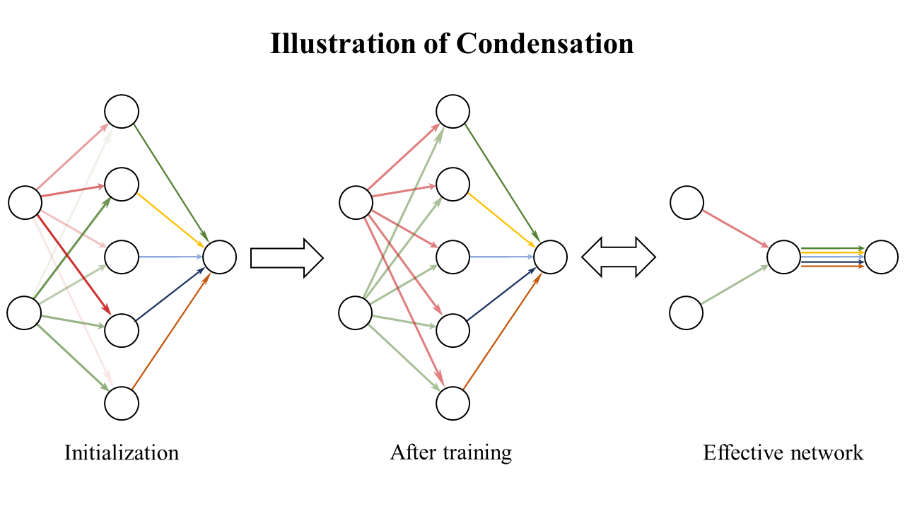
The question why over-parameterized neural networks (NNs) often show good generalization attracts much attention (Breiman, 1995; Zhang et al., 2021). Luo et al. (2021) found that when initialization is small, the input weights of hidden neurons in two-layer ReLU NNs (the input weight or the feature of a hidden neuron consists of the weight from its input layer to the hidden neuron and its bias term) condense onto isolated orientations during the training. As illustrated in the cartoon example in Fig. 1, the condensation transforms a large network, which is often over-parameterized, to the one of only a few effective neurons, leading to an output function with low complexity. Since, in most cases, the complexity bounds the generalization error (Bartlett and Mendelson, 2002), the study of condensation could provide insight to how over-parameterized NNs are implicitly regularized to achieve good generalization performance in practice.

Small initialization leads NNs to rich non-linearity during the training (Mei et al., 2019; Rotskoff and Vanden-Eijnden, 2018; Chizat and Bach, 2018; Sirignano and Spiliopoulos, 2020). For example, in over-parameterized regime, small initialization can achieve low generalization error (Advani et al., 2020). Irrespective of network width, small initialization can make two-layer ReLU NNs converge to a solution with maximum margin (Phuong and Lampert, 2020). Small initialization also enables neural networks to learn features actively (Lyu et al., 2021; Luo et al., 2021). The gradual increment of the condensed orientations is consistent with many previous works, which show that the network output evolves from simple to complex during the training process (Xu et al., 2020; Rahaman et al., 2019; Arpit et al., 2017). The initial condensation resets the network to a simple state, which brings out the simple to complex training process. Condensation is an important phenomenon that reflects the feature learning process. Therefore, it is important to understand how condensation emerges during the training with small initialization.
Refer to caption
Figure 1: Illustration of condensation. The color and its intensity of a line indicate the strength of the weight. Initially, weights are random. Soon after training, the weights from an input node to all hidden neurons are the same, i.e., condensation. Multiple hidden neurons can be replaced by an effective neuron with low complexity, which has the same input weight as original hidden neurons and the output weight as the summation of all output weights of original hidden neurons.

The dynamic behavior of the training at the initial state is important for the whole training process, because it largely determines the training dynamics of a neural network and the region it ends up in (Fort et al., 2020; Hu et al., 2020), which impacts the characteristics of the neural networks in the final stage of training (Luo et al., 2021; Jiang et al., 2019; Li et al., 2018). For two-layer ReLU NNs, several works have studied the mechanism underlying the condensation at the initial training stage when the initialization of parameters goes to zero (Maennel et al., 2018; Pellegrini and Biroli, 2020). However, it still remains unclear that for NNs of more general activation functions, how the condensation emerges at the initial training stage.

In this work, we show that the condensation at the initial stage is closely related to the multiplicity p𝑝p at x=0𝑥0x=0, which means the derivative of activation at x=0𝑥0x=0 is zero up to the (p1)th𝑝1𝑡(p-1)th-order and is non-zero for the p𝑝p-th order. Many common activation functions, e.g., tanh(x)𝑥\tanh(x), sigmoid(x)sigmoid𝑥\mathrm{sigmoid}(x), softplus(x)softplus𝑥\mathrm{softplus}(x), Gelu(x)Gelu𝑥\mathrm{Gelu}(x), Swich(x)Swich𝑥\mathrm{Swich}(x), etc, are all multiplicity p=1𝑝1p=1, and xtanh(x)𝑥𝑥x\tanh(x) and x2tanh(x)superscript𝑥2𝑥x^{2}\tanh(x) have multiplicity two and three, respectively. Our contribution is summarized as follows:

  • Our extensive experiments suggest that the maximal number of condensed orientations in the initial training is twice the multiplicity of the activation function used in general NNs.

  • We present a theory for the initial condensation with small initialization for two cases, one is for the activation function of multiplicity one with arbitrary dimension input, and the other is for the layer with one-dimensional input and arbitrary multiplicity. As many common activation functions are multiplicity p=1𝑝1p=1, our theory would be of interest to general readers.

2 Related works

Luo et al. (2021) systematically study the effect of initialization for two-layer ReLU NN with infinite width by establishing a phase diagram, which shows three distinct regimes, i.e., linear regime (similar to the lazy regime)  (Jacot et al., 2018; Arora et al., 2019; Zhang et al., 2020; E et al., 2020; Chizat and Bach, 2019), critical regime (Mei et al., 2019; Rotskoff and Vanden-Eijnden, 2018; Chizat and Bach, 2018; Sirignano and Spiliopoulos, 2020) and condensed regime (non-linear regime), based on the relative change of input weights as the width approaches infinity, which tends to 00, O(1)𝑂1O(1) and ++\infty, respectively. Zhou et al. (2022) make a step towards drawing a phase diagram for three-layer ReLU NNs with infinite width, revealing the possibility of completely different dynamics (linear, critical and condensed dynamics) emerging within a deep NN for its different layers. As shown in Luo et al. (2021), two-layer ReLU NNs with infinite width do not condense in the neural tangent kernel (NTK) regime , slightly condense in the mean-field regime, and clearly condense in the non-linear regime. However, in Luo et al. (2021), it is not clear how general the condensation phenomenon is when other activation functions are used and why there is condensation.

Zhang et al. (2021a, b); Fukumizu and Amari (2000); Fukumizu et al. (2019); Simsek et al. (2021) propose a general Embedding Principle of loss landscape of DNNs that unravels a hierarchical structure of the loss landscape of NNs, i.e., loss landscape of an DNN contains all critical points of all the narrower DNNs. The embedding principle shows that a large DNN can experience critical points where the DNN condenses and its output is the same as that of a much smaller DNN. However, the embedding principle does not explain how the training can take the DNN to such critical points.

The condensation is consistent with previous works that suggest that NNs may learn data from simple to complex patterns (Arpit et al., 2017; Xu et al., 2019; Rahaman et al., 2019; Xu et al., 2020; Jin et al., 2020; Kalimeris et al., 2019). For example, an implicit bias of frequency principle is widely observed that NNs often learn the target function from low to high frequency (Xu et al., 2019; Rahaman et al., 2019; Xu et al., 2020), which has been utilized to understand various phenomena (Ma et al., 2020; Xu and Zhou, 2021) and inspired algorithm design (Liu et al., 2020; Cai et al., 2020; Tancik et al., 2020; Li et al., 2020, 2021).

3 Preliminary: Neural networks and initial stage

A two-layer NN is

f𝜽(𝒙)=j=1majσ(𝒘j𝒙),subscript𝑓𝜽𝒙superscriptsubscript𝑗1𝑚subscript𝑎𝑗𝜎subscript𝒘𝑗𝒙f_{\bm{\theta}}(\bm{x})=\sum_{j=1}^{m}a_{j}\sigma(\bm{w}_{j}\cdot\bm{x}), (1)

where σ()𝜎\sigma(\cdot) is the activation function, 𝒘j=(𝒘¯j,𝒃j)d+1subscript𝒘𝑗subscript¯𝒘𝑗subscript𝒃𝑗superscript𝑑1\bm{w}_{j}=(\bar{\bm{w}}_{j},\bm{b}_{j})\in\mathbb{R}^{d+1} is the neuron feature including the input weight and bias terms, and 𝒙=(𝒙¯,1)d+1𝒙¯𝒙1superscript𝑑1\bm{x}=(\bar{\bm{x}},1)\in\mathbb{R}^{d+1} is the concatenation of the input sample and scalar 111, 𝜽𝜽\bm{\theta} is the set of all parameters, i.e., {aj,𝒘j}j=1msuperscriptsubscriptsubscript𝑎𝑗subscript𝒘𝑗𝑗1𝑚\{a_{j},\bm{w}_{j}\}_{j=1}^{m}. For simplicity, we call wjsubscript𝑤𝑗\bm{w}_{j} input weight or weight and 𝒙𝒙\bm{x} input sample.

A L𝐿L-layer NN can be recursively defined by setting the output of the previous layer as the input to the current hidden layer, i.e.,

𝒙[0]=(𝒙,1),𝒙[1]=(σ(𝑾[1]\displaystyle\bm{x}^{[0]}=(\bm{x},1),\quad\bm{x}^{[1]}=(\sigma(\bm{W}^{[1]} 𝒙[0]),1),𝒙[l]=(σ(𝑾[l]𝒙[l1]),1),forl{2,3,,L}\displaystyle\bm{x}^{[0]}),1),\quad\bm{x}^{[l]}=(\sigma(\bm{W}^{[l]}\bm{x}^{[l-1]}),1),\ \text{for}\ l\in\{2,3,...,L\} (2)
f(𝜽,𝒙)=𝒂𝒙[L]f𝜽(𝒙),𝑓𝜽𝒙superscript𝒂superscript𝒙delimited-[]𝐿subscript𝑓𝜽𝒙\displaystyle f(\bm{\theta},\bm{x})=\bm{a}^{\intercal}\bm{x}^{[L]}\triangleq f_{\bm{\theta}}(\bm{x}),

where 𝑾[l]=(𝑾¯[l],𝒃[l])ml×(ml1+1)superscript𝑾delimited-[]𝑙superscript¯𝑾delimited-[]𝑙superscript𝒃delimited-[]𝑙superscriptsubscript𝑚𝑙subscript𝑚𝑙11\bm{W}^{[l]}=(\bar{\bm{W}}^{[l]},\bm{b}^{[l]})\in\mathbb{R}^{m_{l}\times(m_{l-1}+1)}, and mlsubscript𝑚𝑙m_{l} represents the dimension of the l𝑙l-th hidden layer. For simplicity, we also call each row of W[l]superscript𝑊delimited-[]𝑙\bm{W}^{[l]} input weight or weight and 𝒙[l1]superscript𝒙delimited-[]𝑙1\bm{x}^{[l-1]} input to the l𝑙l-th hidden layer. The target function is denoted as f(𝒙)superscript𝑓𝒙f^{*}(\bm{x}). The training loss function is the mean squared error

R(𝜽)=12ni=1n(f𝜽(𝒙i)f(𝒙i))2.𝑅𝜽12𝑛superscriptsubscript𝑖1𝑛superscriptsubscript𝑓𝜽subscript𝒙𝑖superscript𝑓subscript𝒙𝑖2R(\bm{\theta})=\frac{1}{2n}\sum_{i=1}^{n}(f_{\bm{\theta}}(\bm{x}_{i})-f^{*}(\bm{x}_{i}))^{2}. (3)

Without loss of generality, we assume that the output is one-dimensional for theoretical analysis, because, for high-dimensional cases, we only need to sum up the components directly. For summation, it does not affect the results of our theories. We consider the gradient flow training

𝜽˙=𝜽R(𝜽).˙𝜽subscript𝜽𝑅𝜽\dot{\bm{\theta}}=-\nabla_{\bm{\theta}}R(\bm{\theta}). (4)

To ensure that the training is close to the gradient flow, all the learning rates used in this paper are sufficiently small. We characterize the activation function by the following definition.

Definition 1 (multiplicity p𝑝p).

Suppose that σ(x)𝜎𝑥\sigma(x) satisfies the following condition, there exists a p𝑝superscriptp\in\mathbb{N}^{*}, such that the s𝑠s-th order derivative σ(s)(0)=0superscript𝜎𝑠00\sigma^{(s)}(0)=0 for s=1,2,,p1𝑠12𝑝1s=1,2,\cdots,p-1, and σ(p)(0)0superscript𝜎𝑝00\sigma^{(p)}(0)\neq 0, then we say σ𝜎\sigma has multiplicity p𝑝p.

Remark 3.1.

Here are some examples. tanh(x)𝑥\tanh(x), sigmoid(x)sigmoid𝑥\mathrm{sigmoid}(x) and softplus(x)softplus𝑥\mathrm{softplus}(x) have multiplicity p=1𝑝1p=1. xtanh(x)𝑥𝑥x\tanh(x) has multiplicity p=2𝑝2p=2.

We illustrate small initialization and initial stage as follows

Small initialization: 𝑾[l]o(1)similar-tosuperscript𝑾delimited-[]𝑙𝑜1\bm{W}^{[l]}\sim o(1) and 𝑾[l]𝒙[l1]o(1)similar-tosuperscript𝑾delimited-[]𝑙superscript𝒙delimited-[]𝑙1𝑜1\bm{W}^{[l]}\bm{x}^{[l-1]}\sim o(1) for all l𝑙l’s and 𝒙[l1]superscript𝒙delimited-[]𝑙1\bm{x}^{[l-1]}.

We want to remark that it dose not make sense to define the initial stage by the number of training steps, because the training is affected by many factors, such as the learning rate. Therefore, in our experiments, the epochs we use to show phenomena can cover a wide range. Alternatively, we consider the initial stage as follows.

Initial stage: the period when the leading-order Taylor expansion w.r.t activated neurons is still valid for theoretical analysis of Sec. 5.

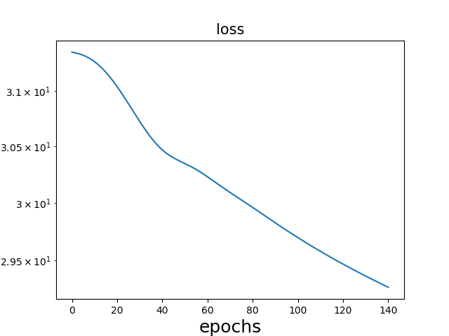
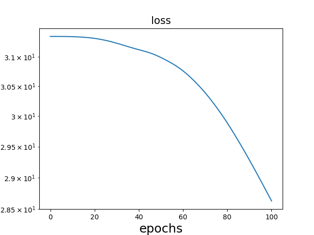
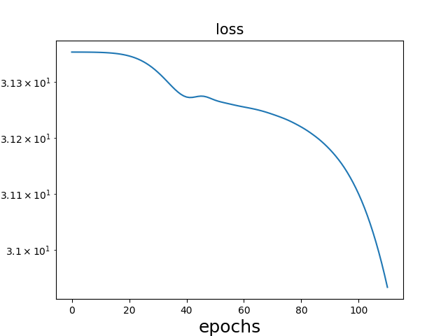
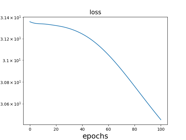
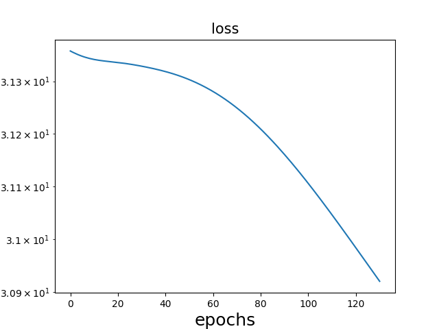
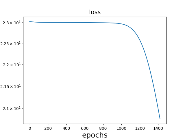
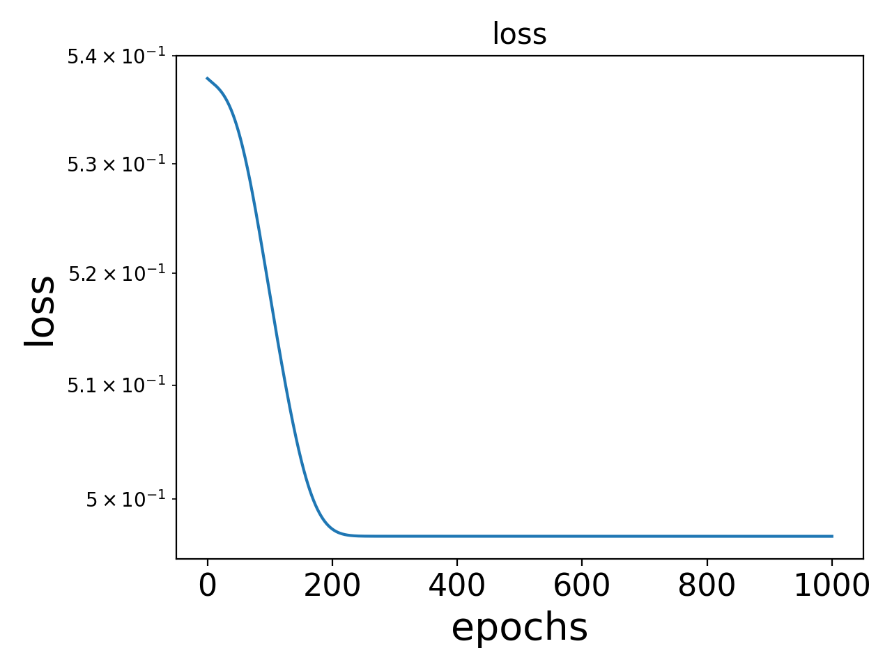
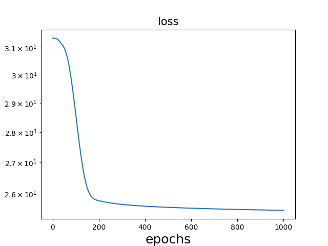
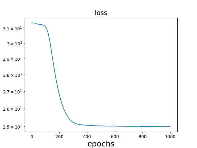
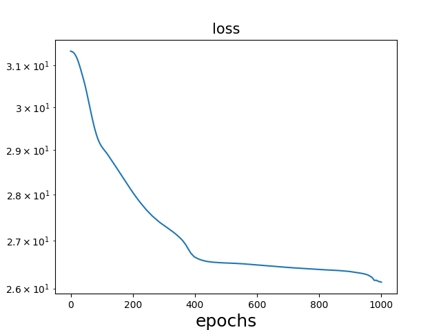
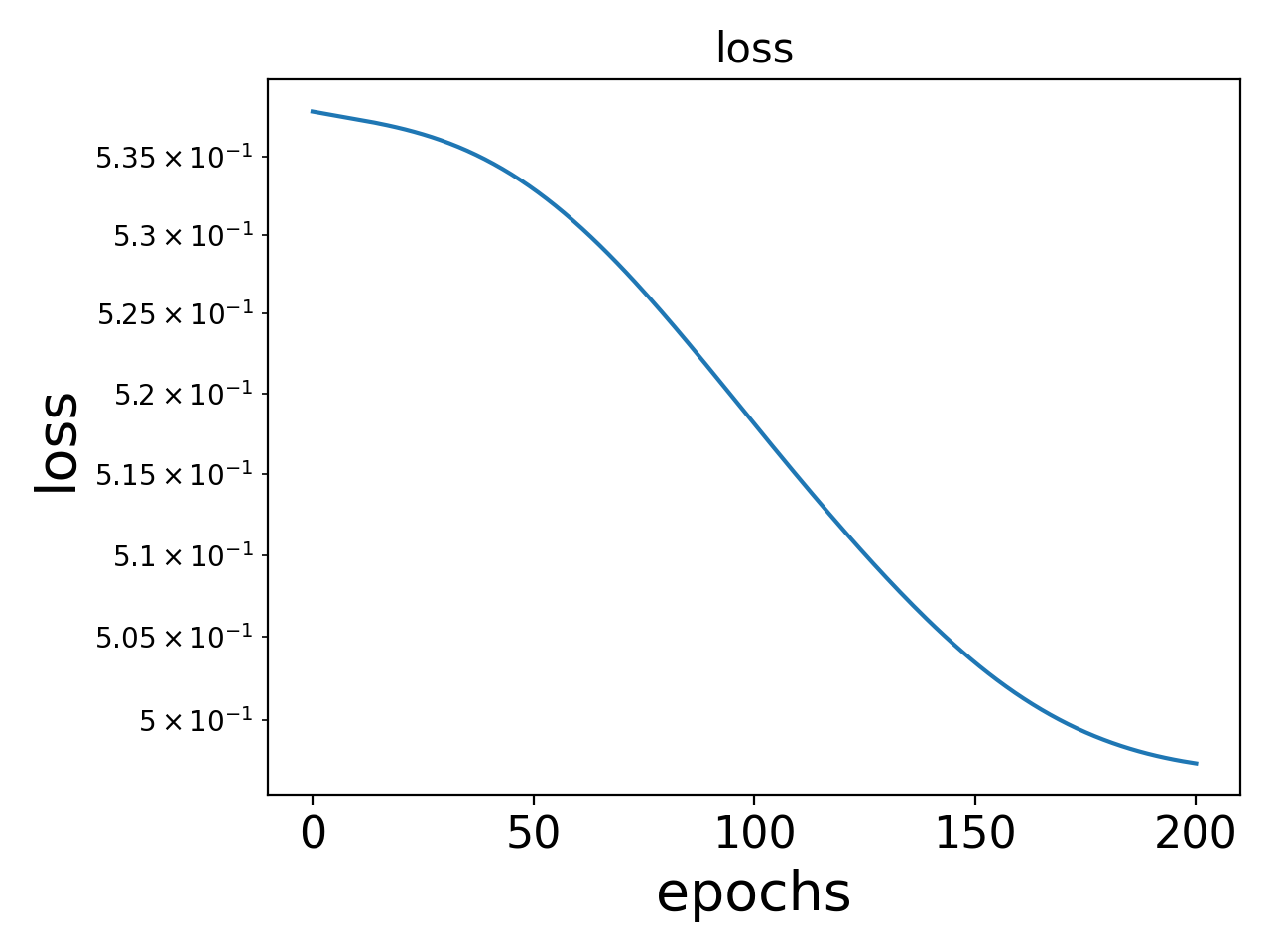
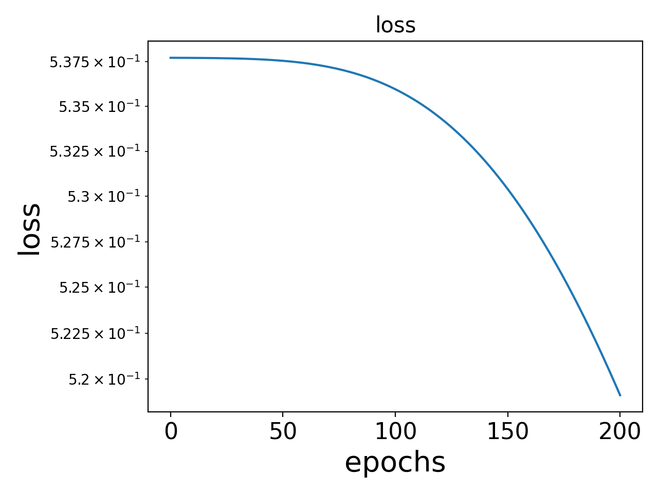
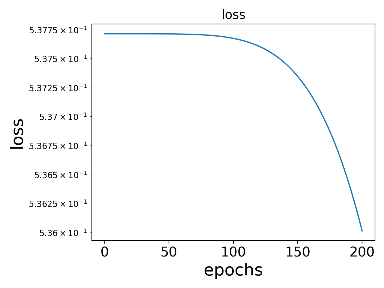
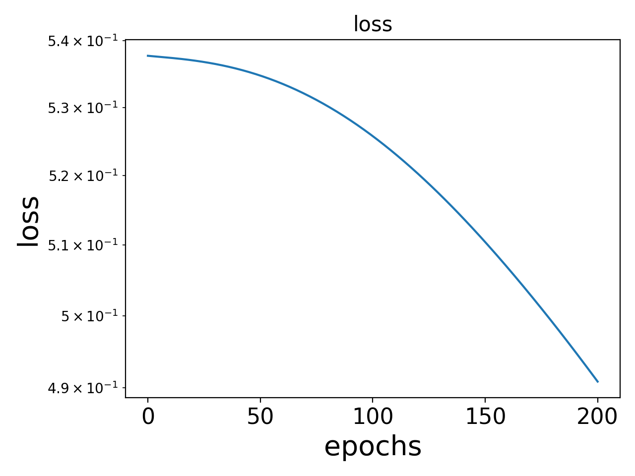
As the parameters of a neural network evolve, the loss value will also decay accordingly, which is easy to be directly observed. Therefore, we propose an intuitive definition of the initial stage of training by the size of loss in this article, that is the stage before the value of loss function decays to 70%percent\% of its initial value. Such a definition is reasonable, for generally a loss could decay to 1%percent\% of its initial value or even lower. The loss of the all experiments in the article can be found in Appendix A.3, and they do meet the definition of the initial stage here.

Cosine similarity: The cosine similarity between two vectors 𝒖𝒖\bm{u} and 𝒗𝒗\bm{v} is defined as

D(𝒖,𝒗)=𝒖𝒗(𝒖𝒖)1/2(𝒗𝒗)1/2.𝐷𝒖𝒗superscript𝒖𝒗superscriptsuperscript𝒖𝒖12superscriptsuperscript𝒗𝒗12D(\bm{u},\bm{v})=\frac{\bm{u}^{\intercal}\bm{v}}{(\bm{u}^{\intercal}\bm{u})^{1/2}(\bm{v}^{\intercal}\bm{v})^{1/2}}. (5)

4 Initial condensation of input weights

In this section, we would empirically show how the condensation differs among NNs with activation function of different multiplicities in the order of a practical example, multidimensional synthetic data, and 1-d input synthetic data, followed by theoretical analysis in the next section.

4.1 Experimental setup

For synthetic dataset: Throughout this work, we use fully-connected neural network with size, d𝑑d-m𝑚m-\cdots-m𝑚m-doutsubscript𝑑outd_{\mathrm{out}}. The input dimension d𝑑d is determined by the training data. The output dimension is dout=1subscript𝑑out1d_{\mathrm{out}}=1. The number of hidden neurons m𝑚m is specified in each experiment. All parameters are initialized by a Gaussian distribution N(0,var)𝑁0varN(0,\mathrm{var}). The total data size is n𝑛n. The training method is Adam with full batch, learning rate lrlr\mathrm{lr} and MSE loss. We sample the training data uniformly from a sub-domain of dsuperscript𝑑\mathbb{R}^{d}. The sampling range and the target function are chosen randomly to show the generality of our experiments.

For CIFAR10 dataset: We use Resnet18-like neural network, which has been described in Fig. 2, and the input dimension is d=32×32×3𝑑32323d=32\times 32\times 3. The output dimension is dout=10subscript𝑑out10d_{\mathrm{out}}=10. All parameters are initialized by a Gaussian distribution N(0,var)𝑁0varN(0,\mathrm{var}). The total data size is n𝑛n. The training method is Adam with batch size 128, learning rate lrlr\mathrm{lr} and cross-entropy loss.

4.2 A practical example

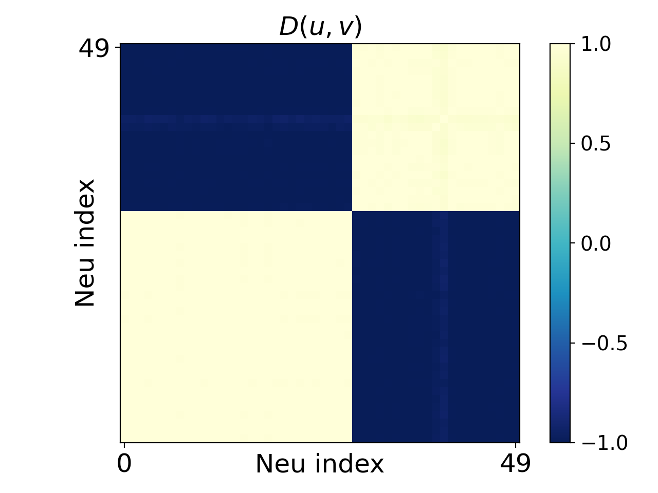
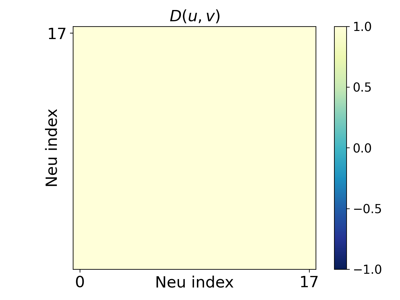
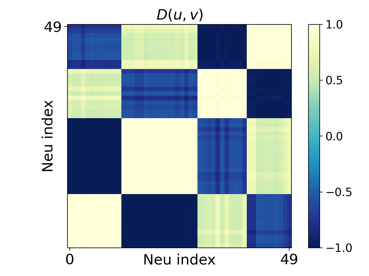
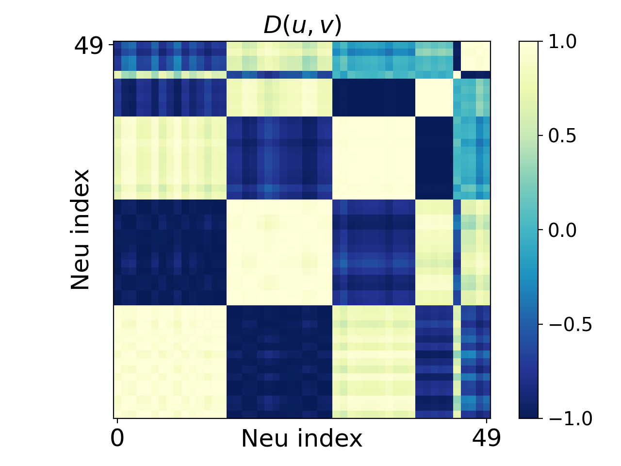
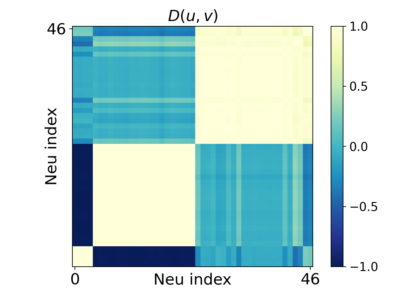
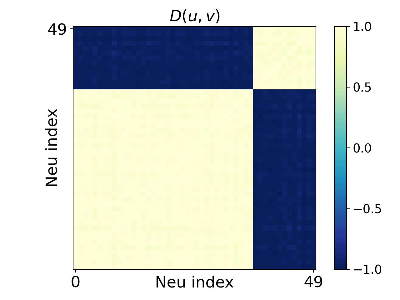
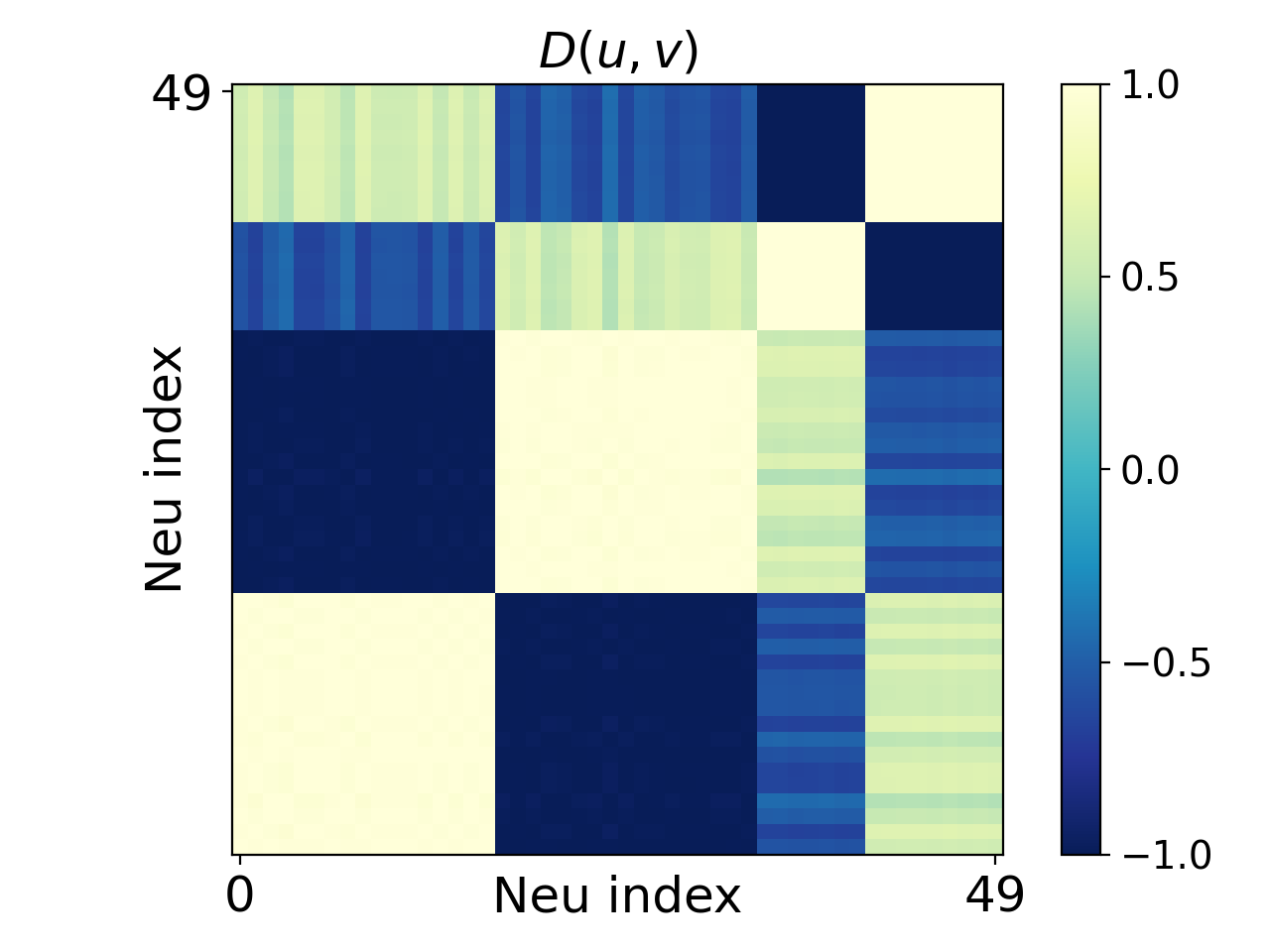
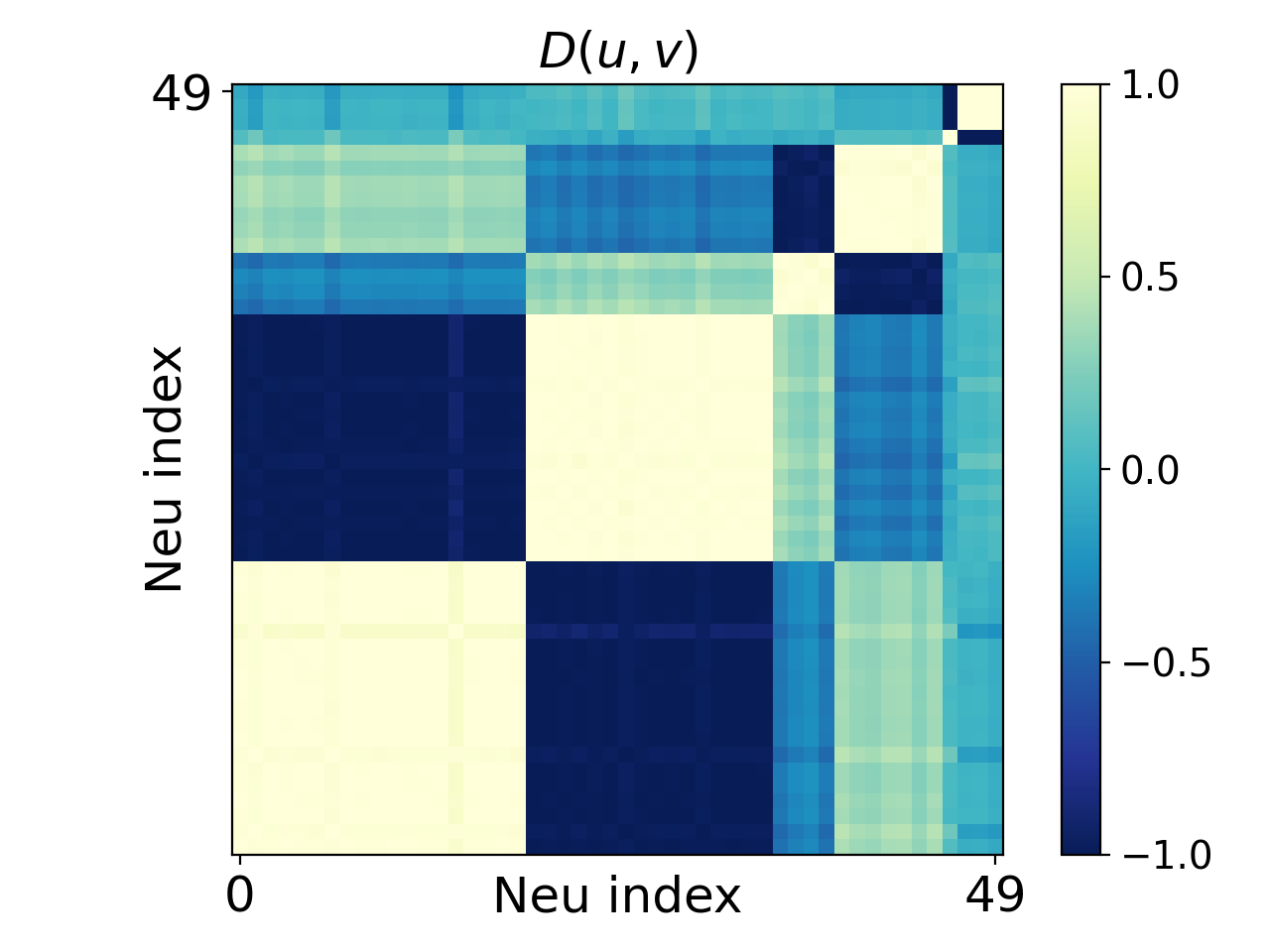
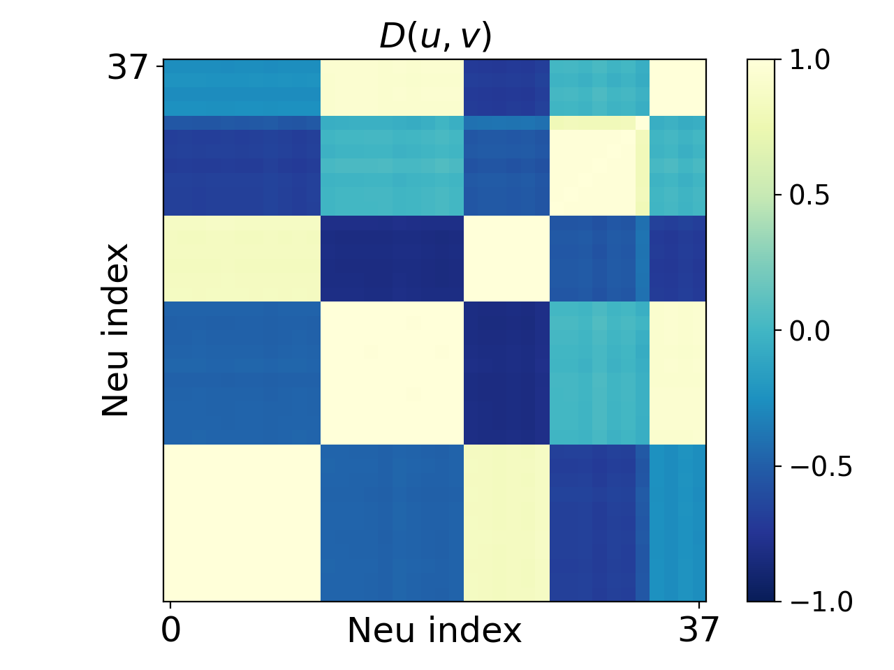
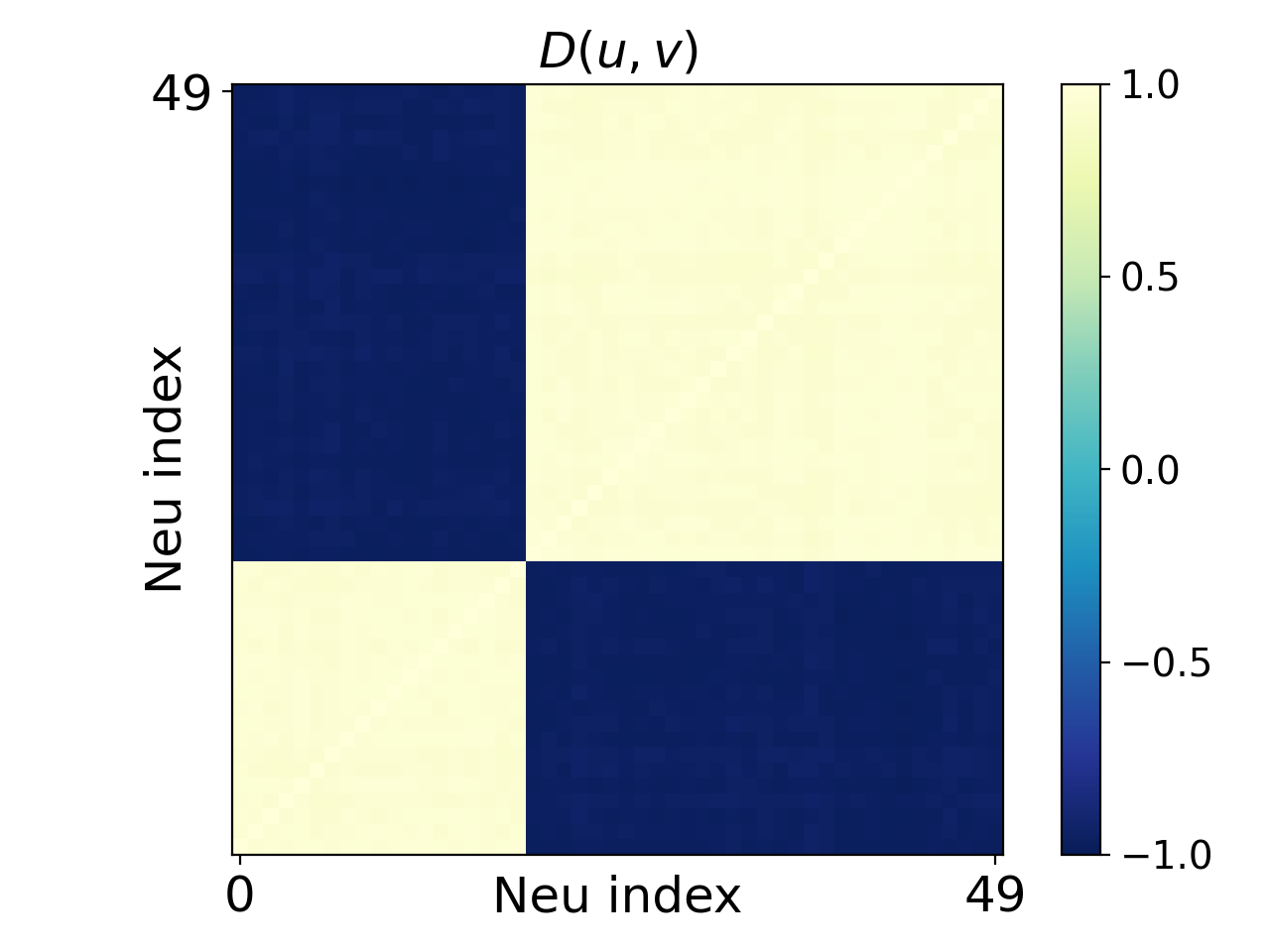
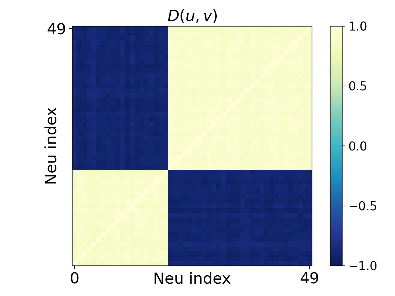
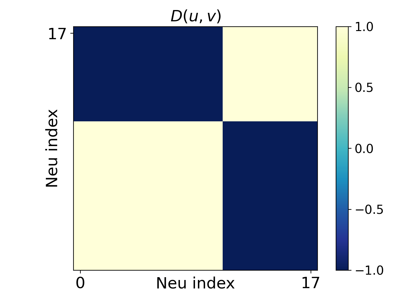
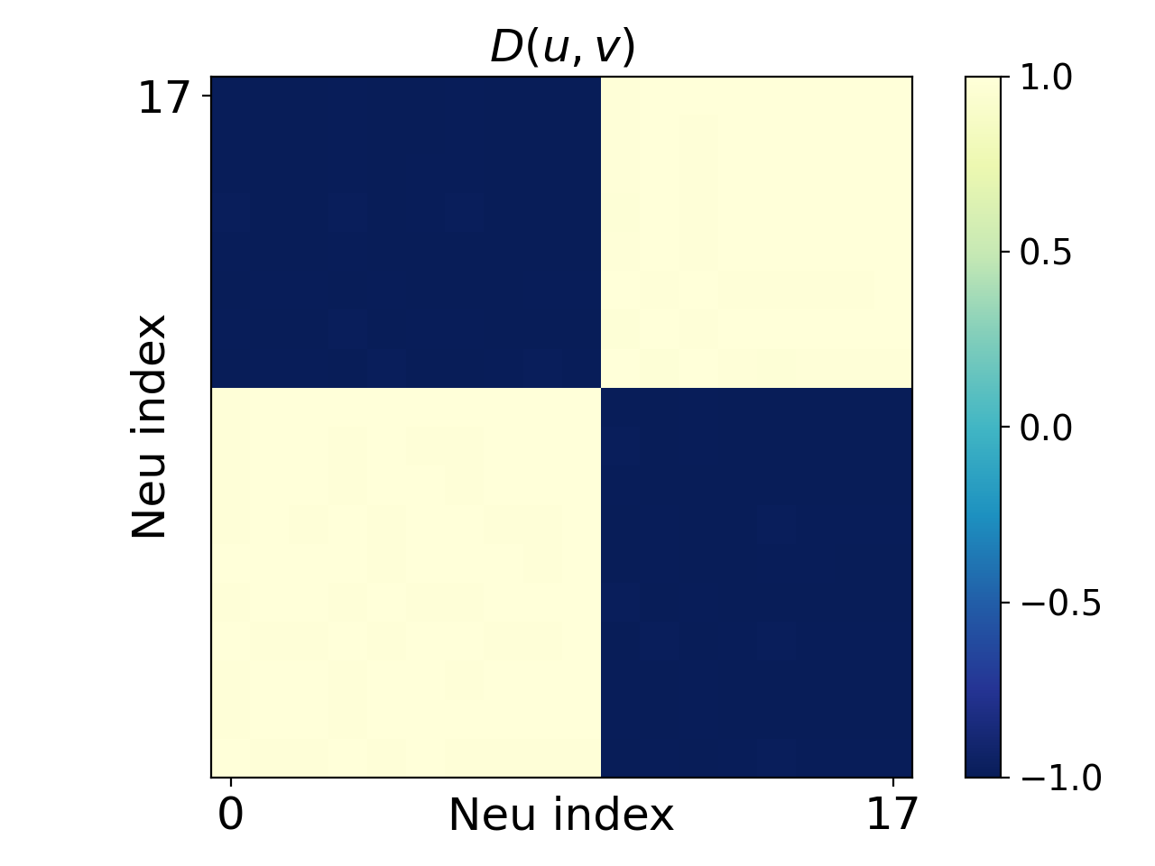
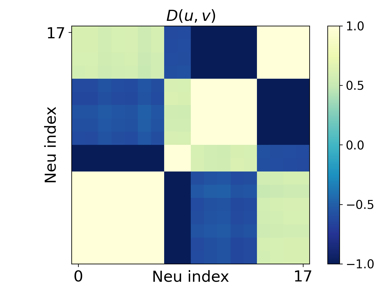
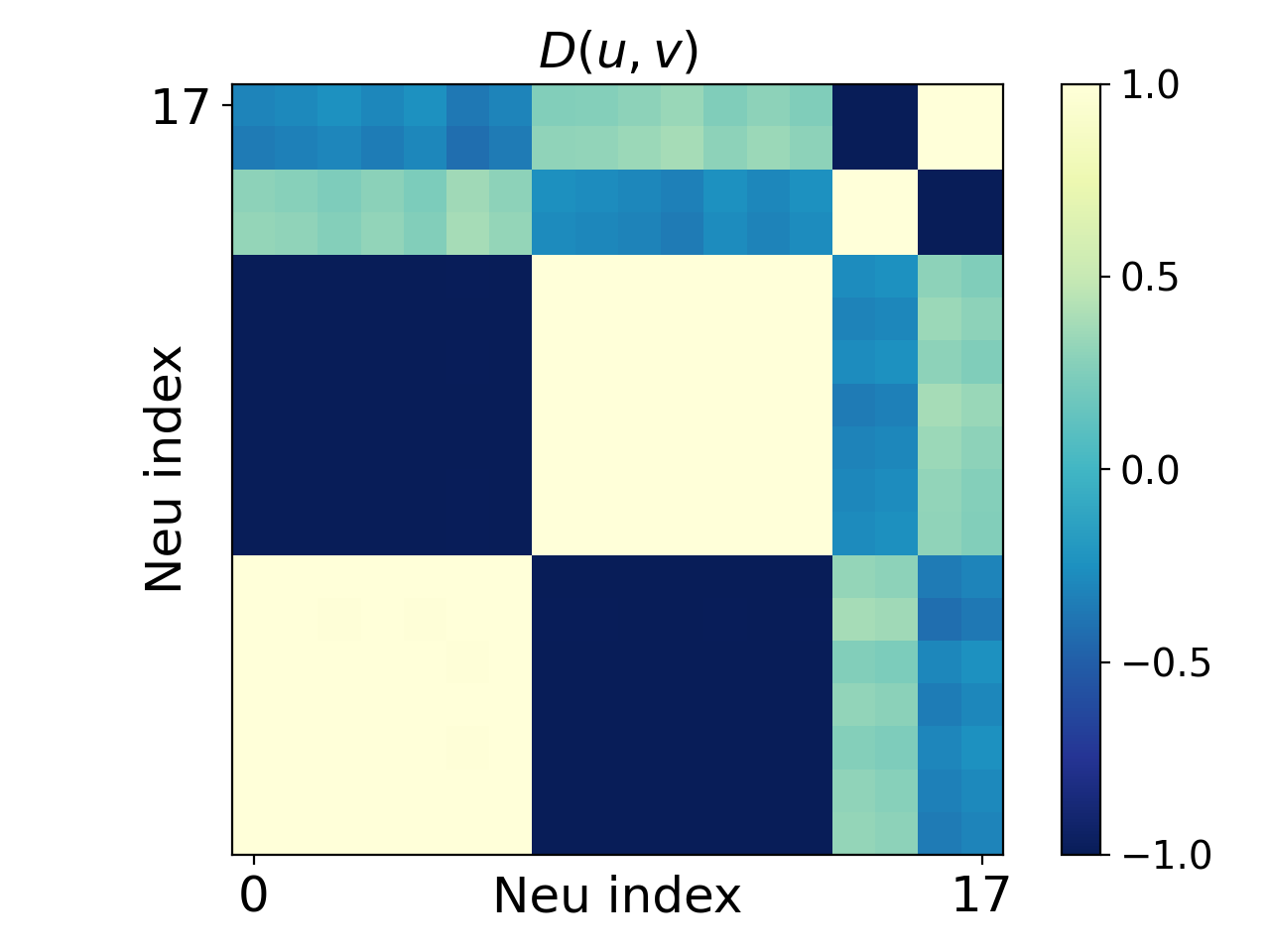
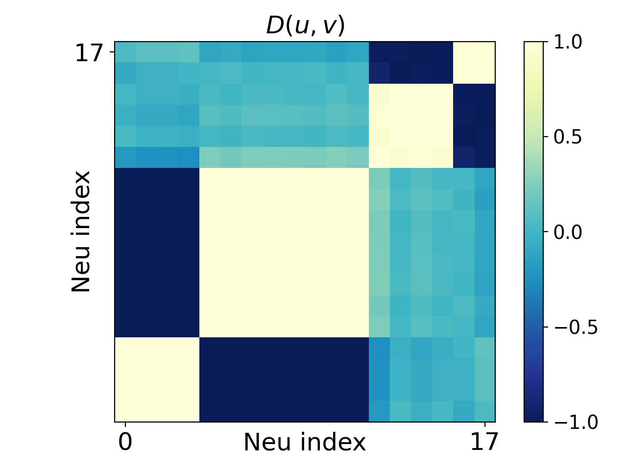
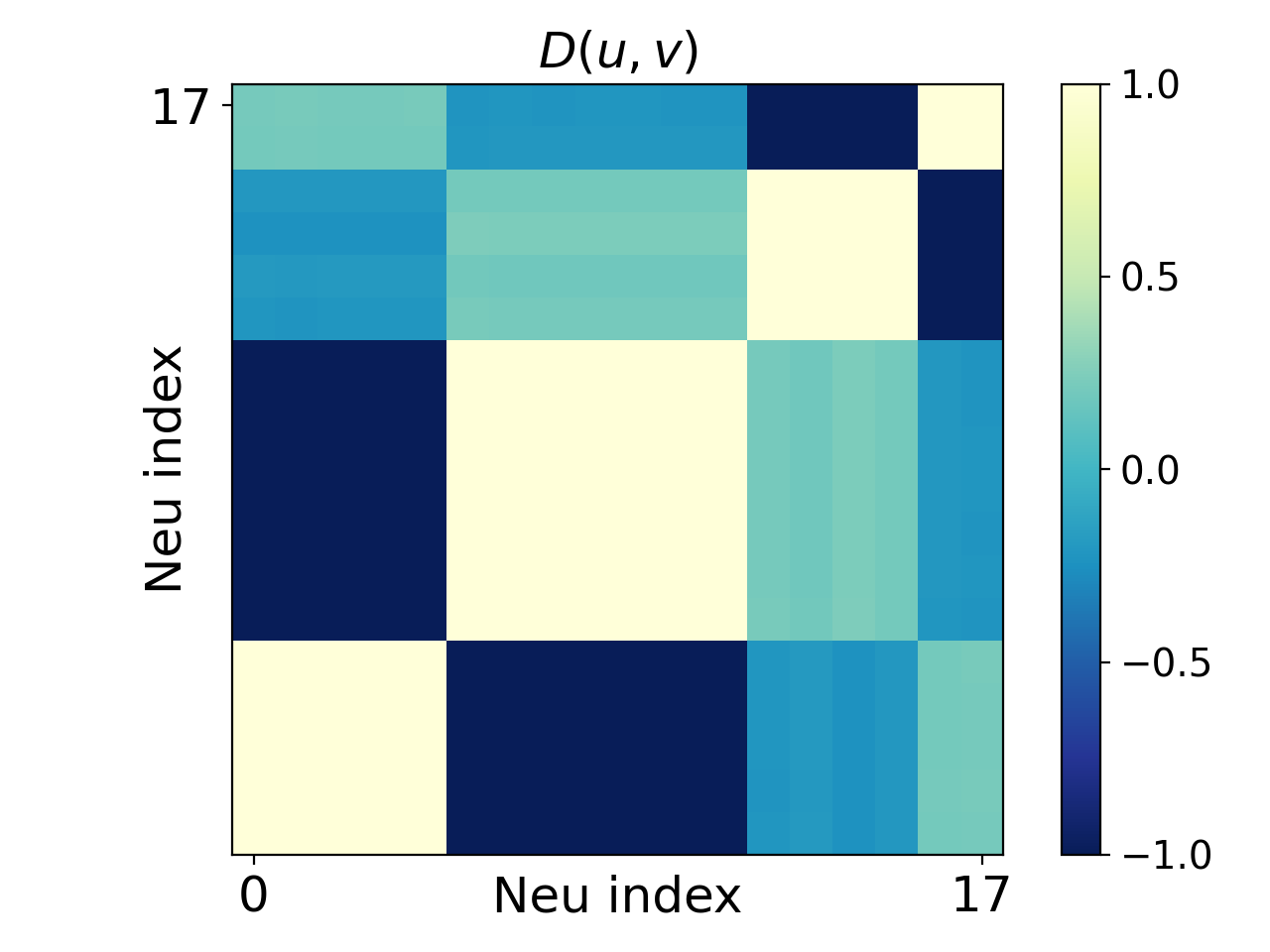
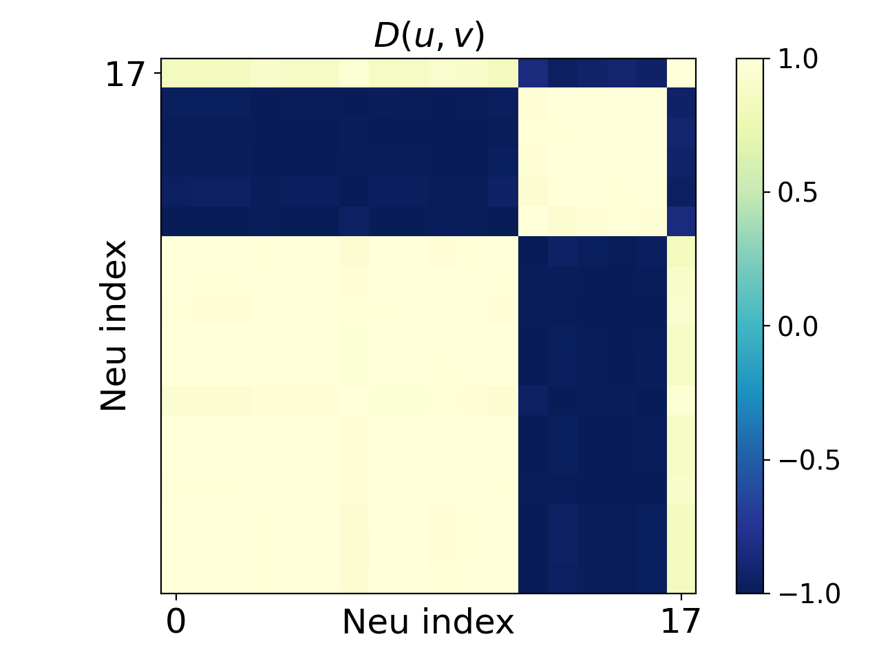
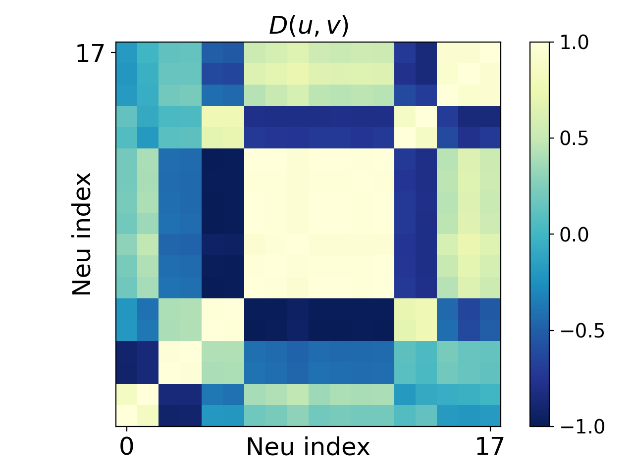
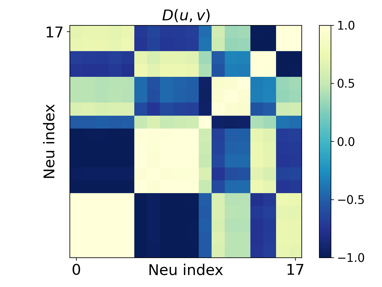
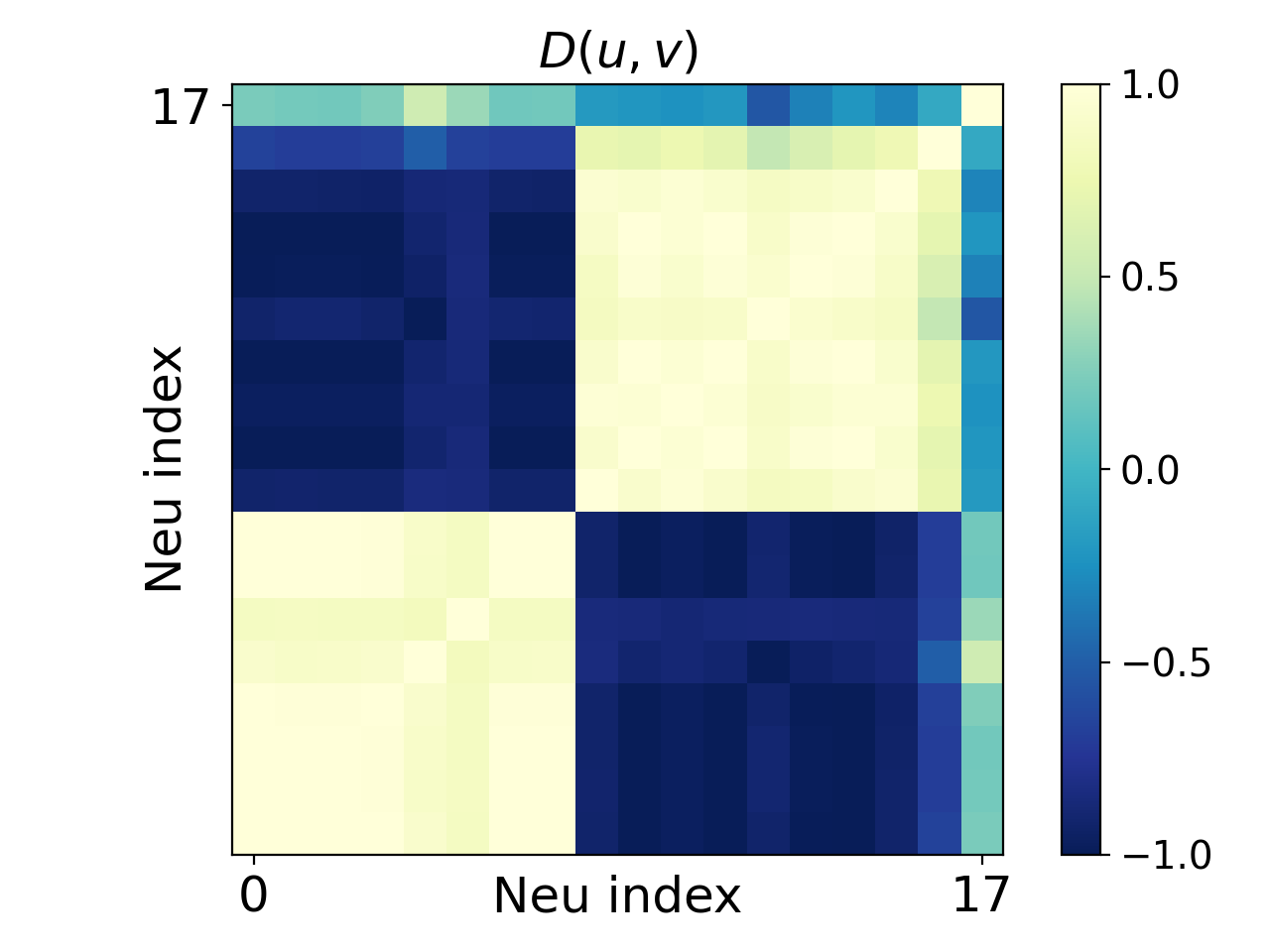
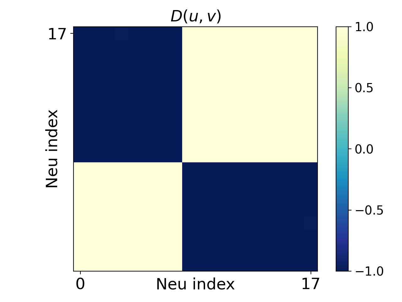
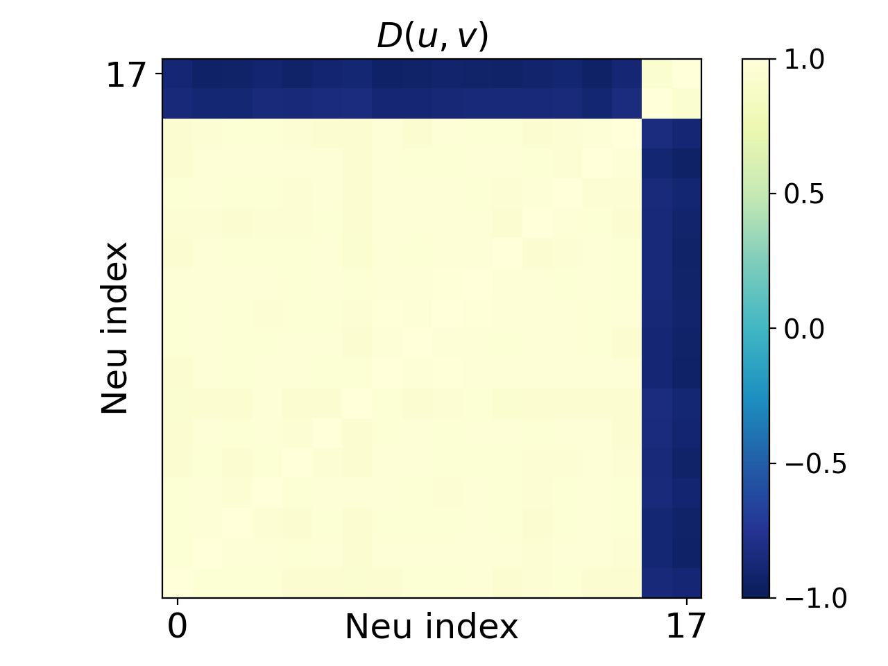
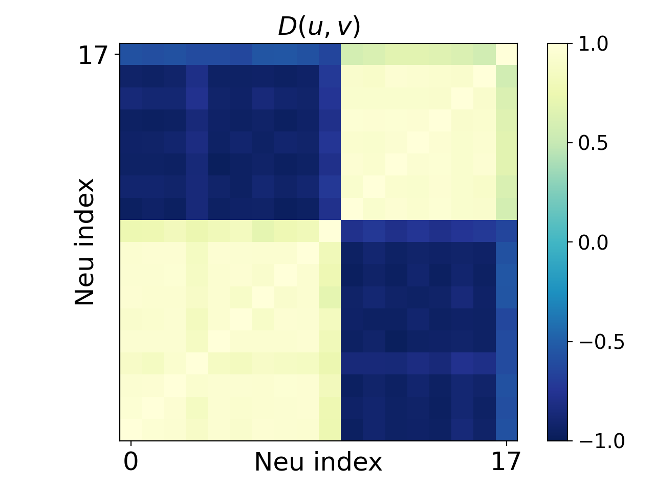
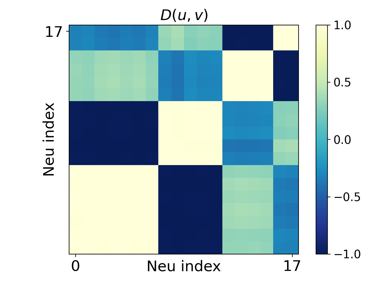
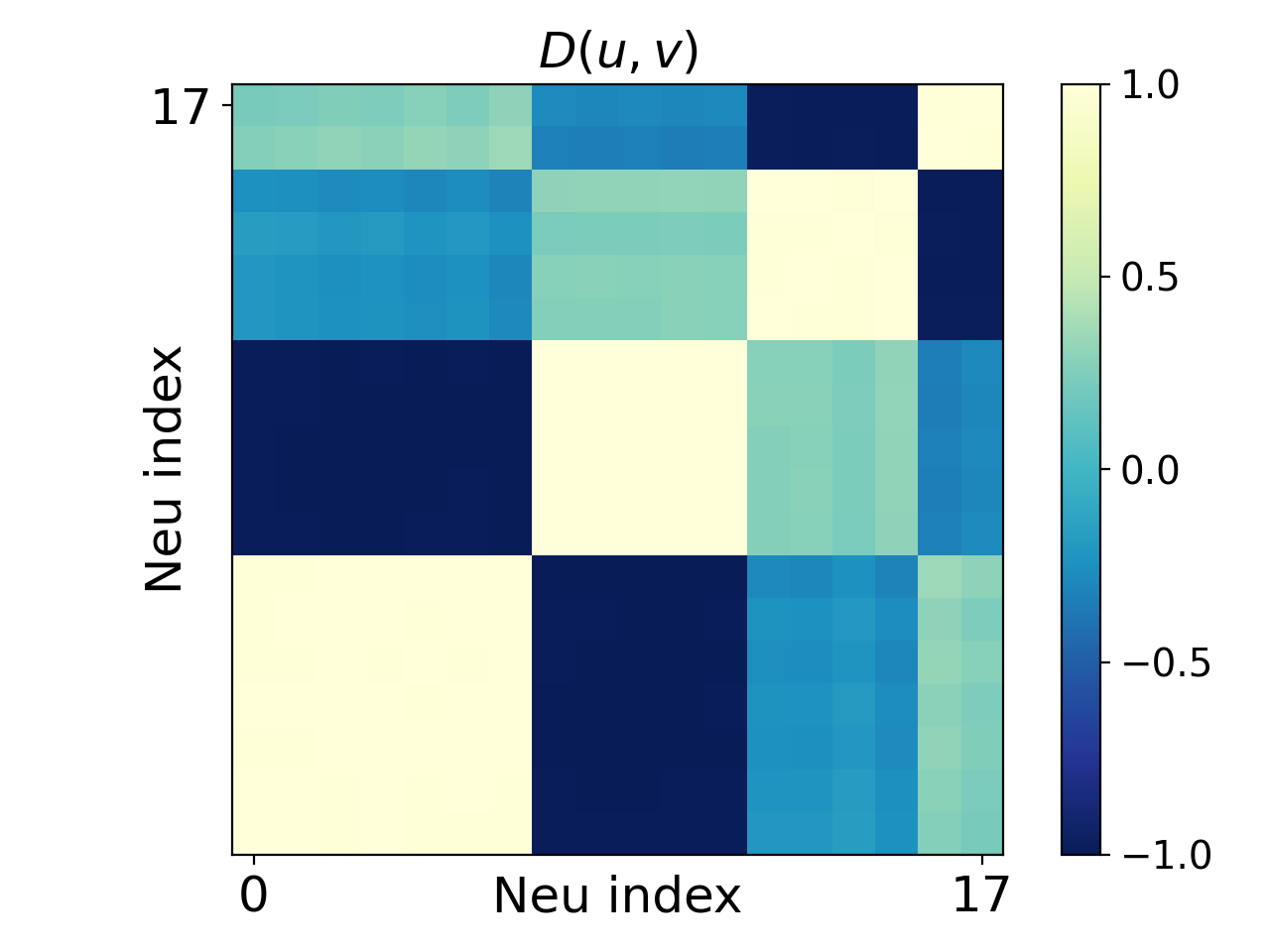
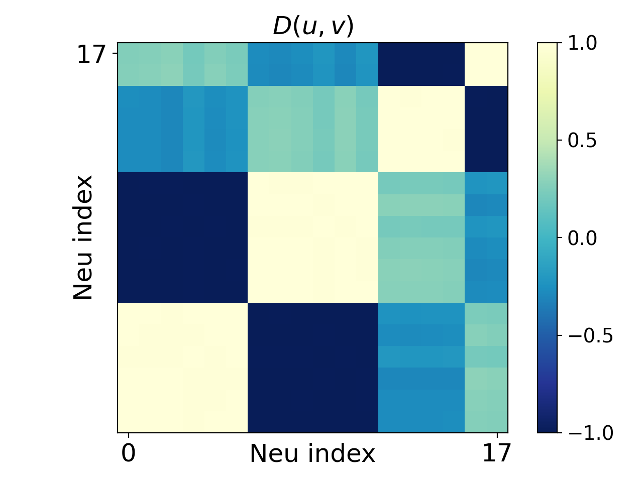
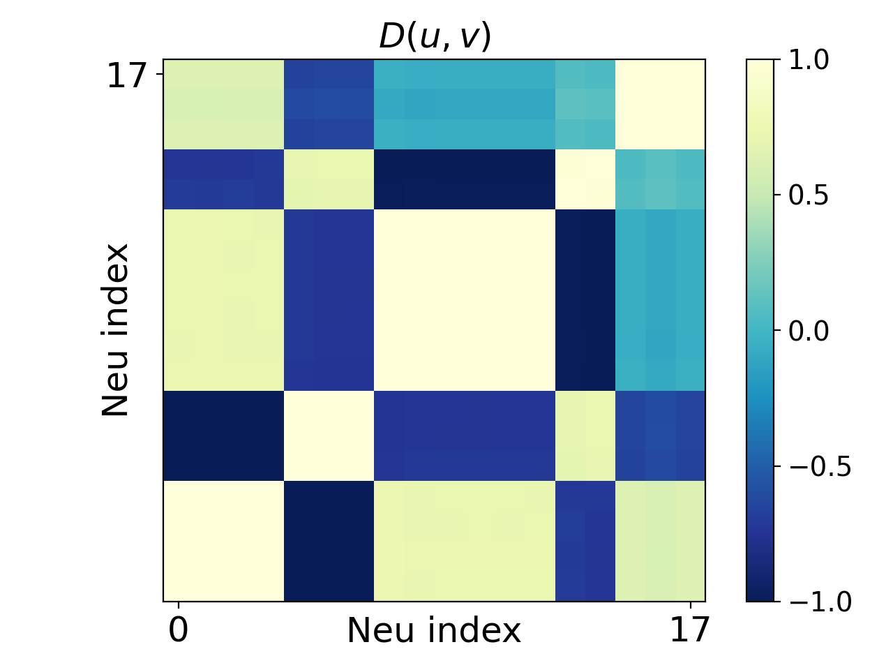
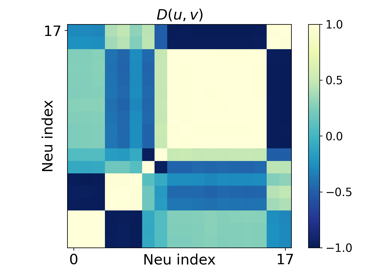
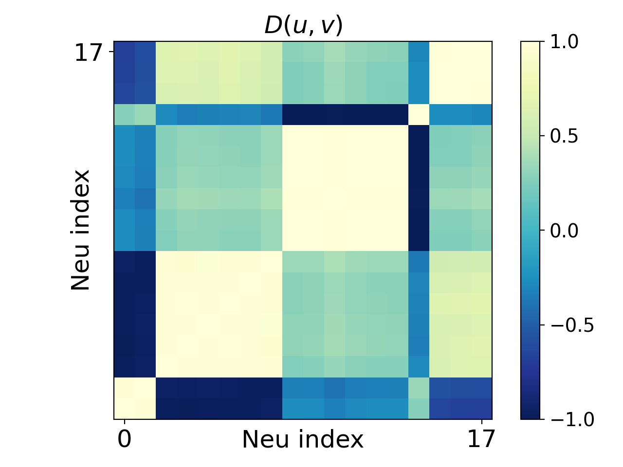
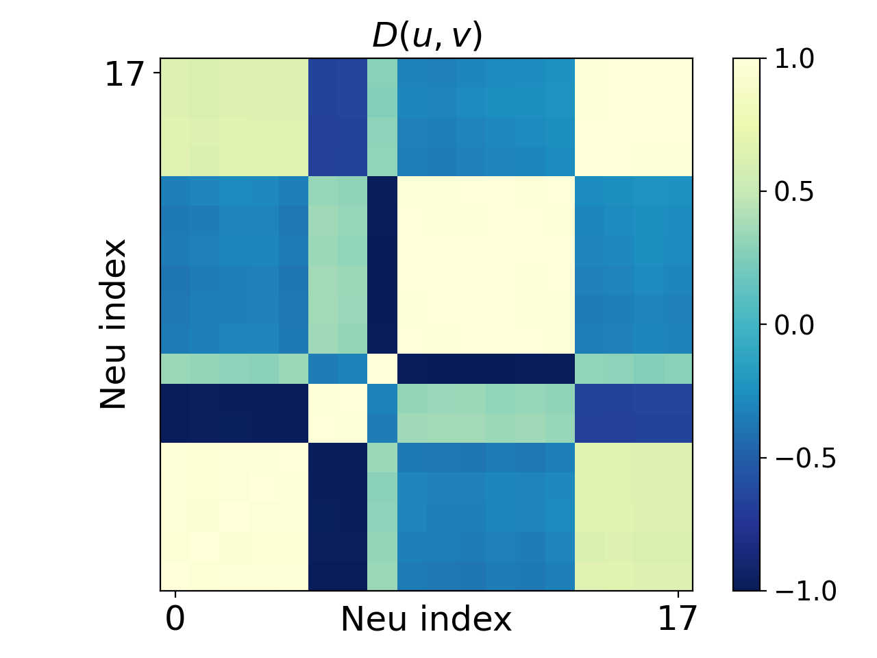
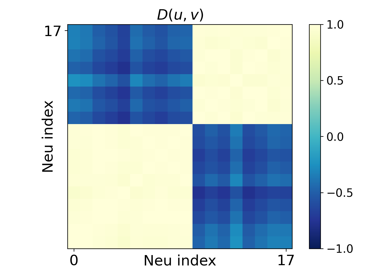
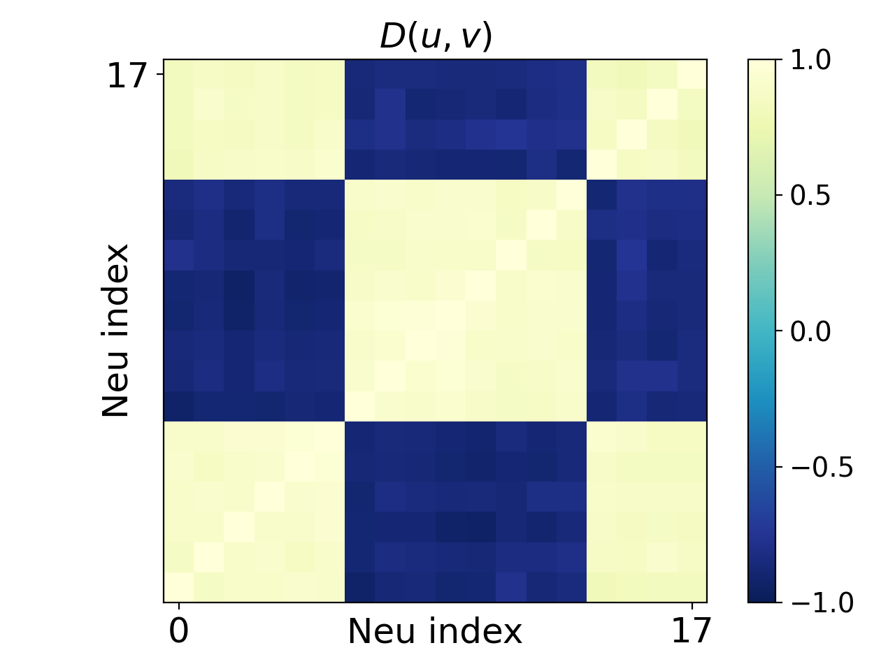
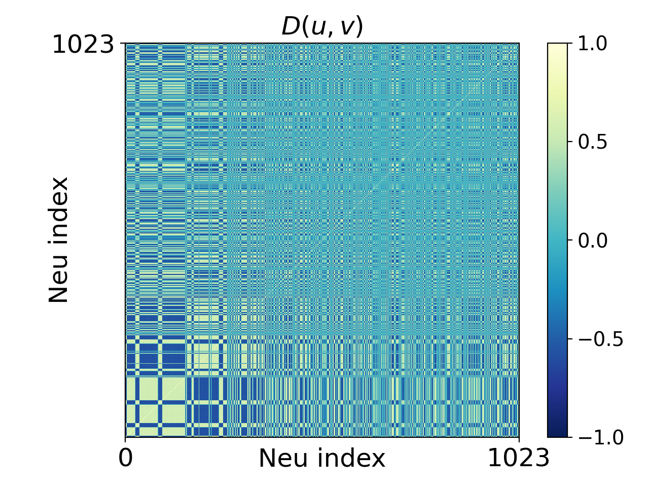
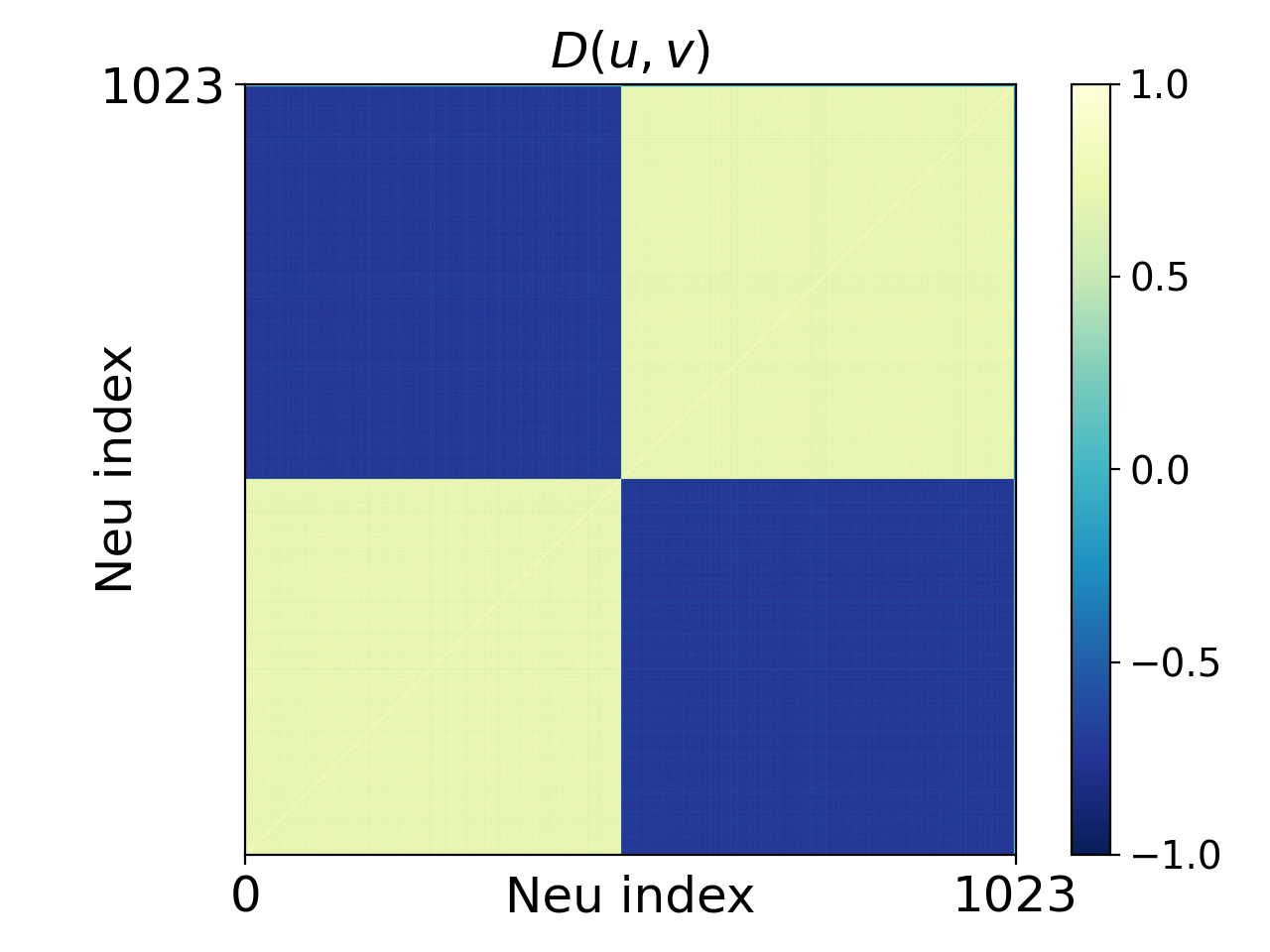
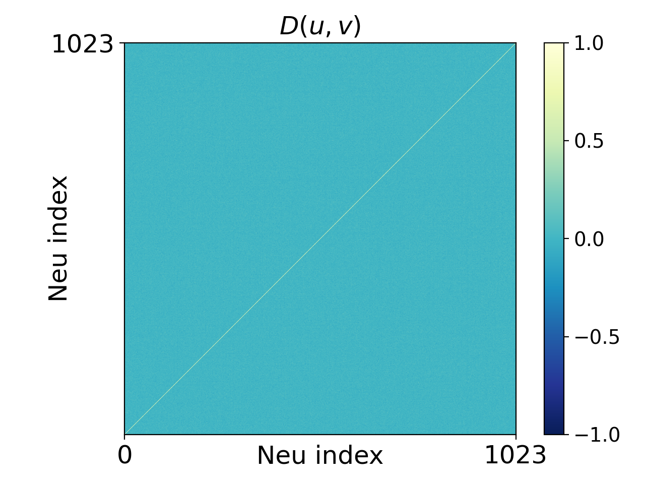
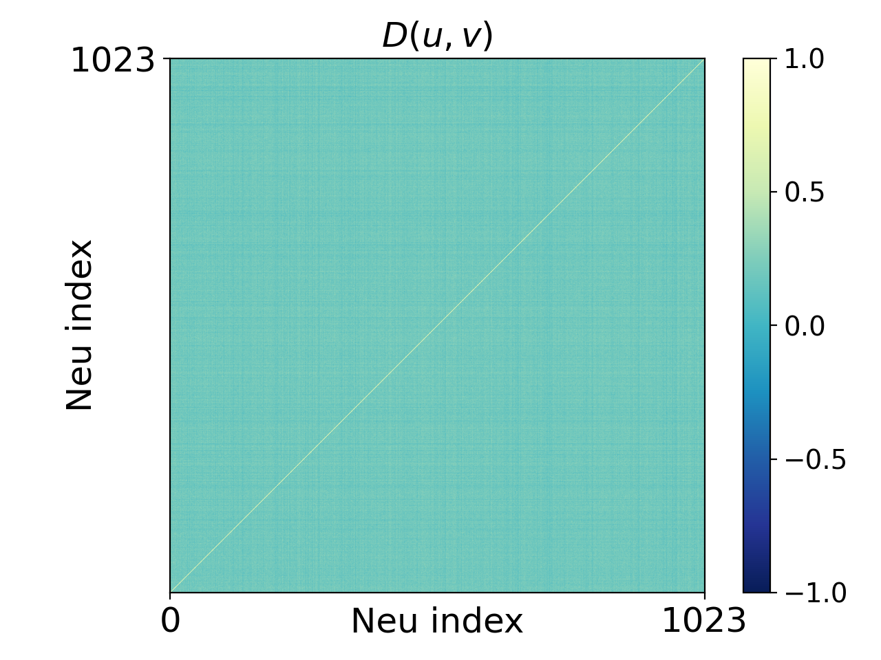
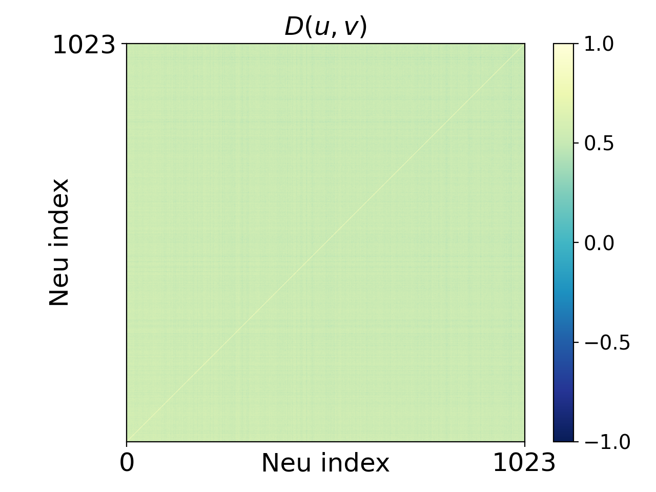
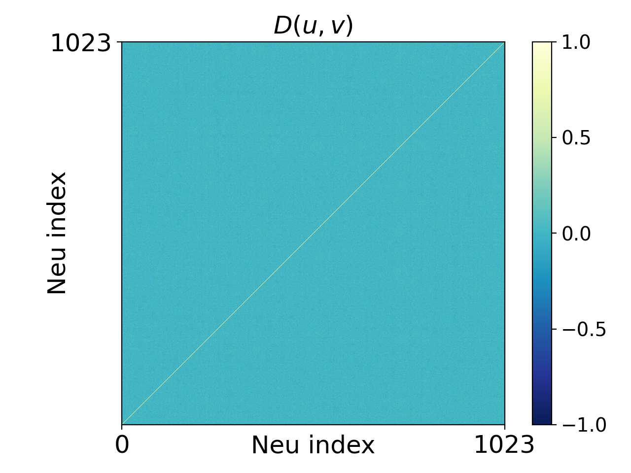
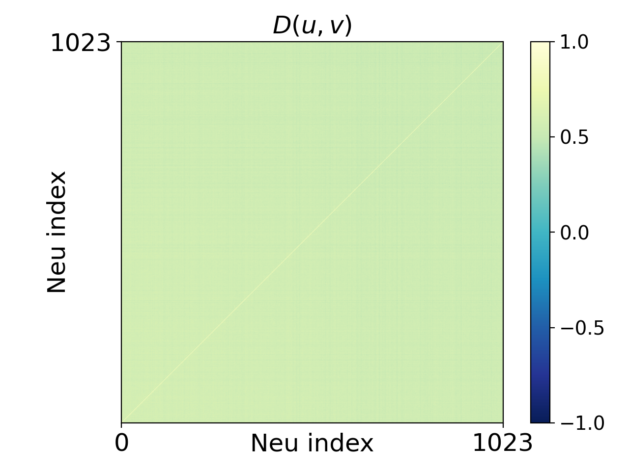
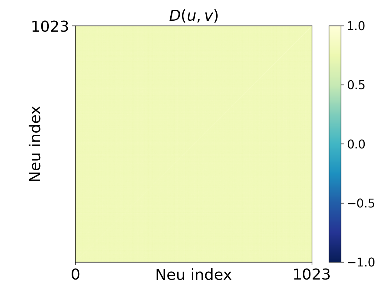
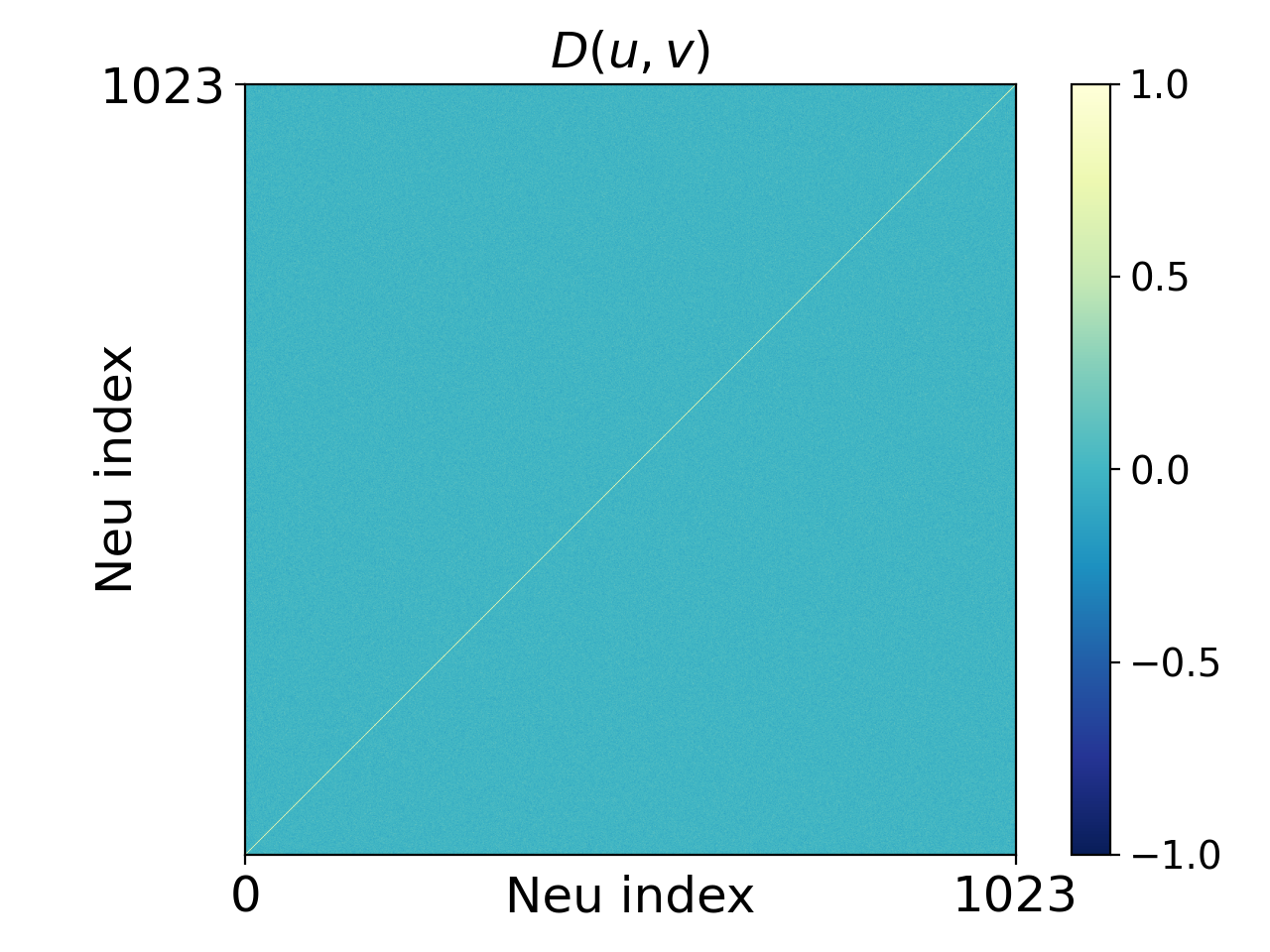
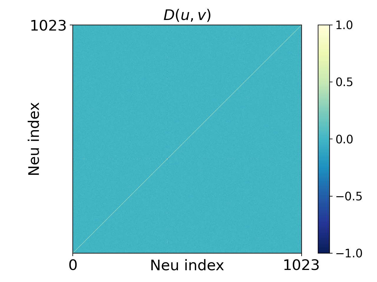
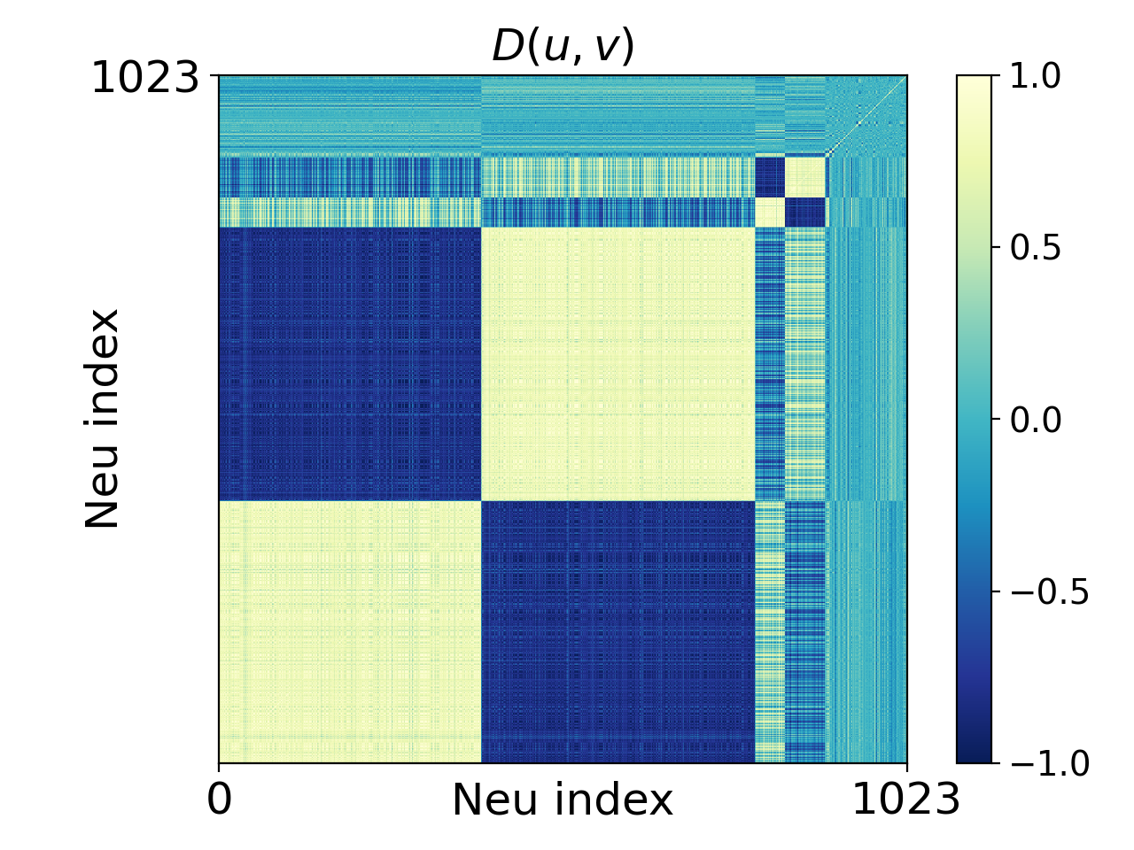
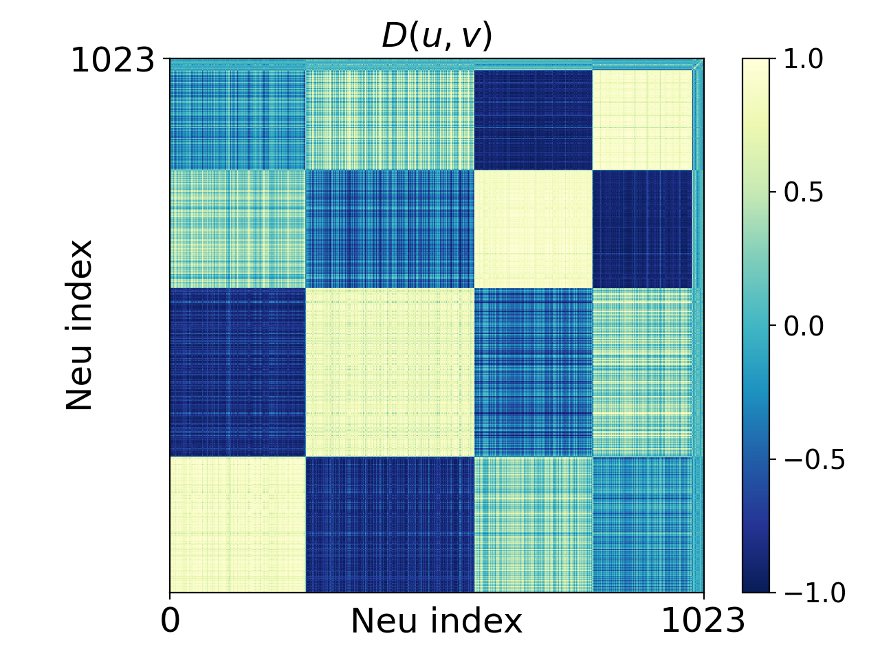
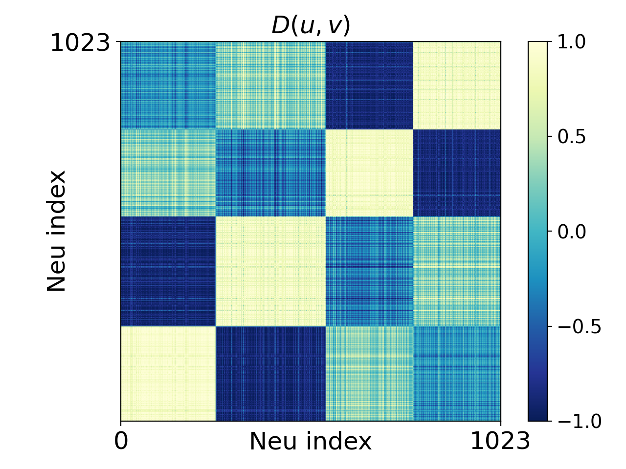
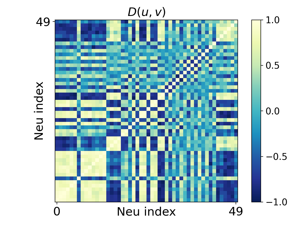
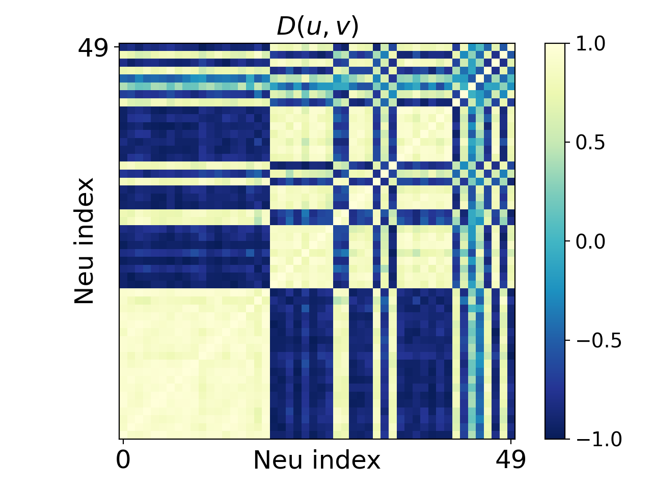
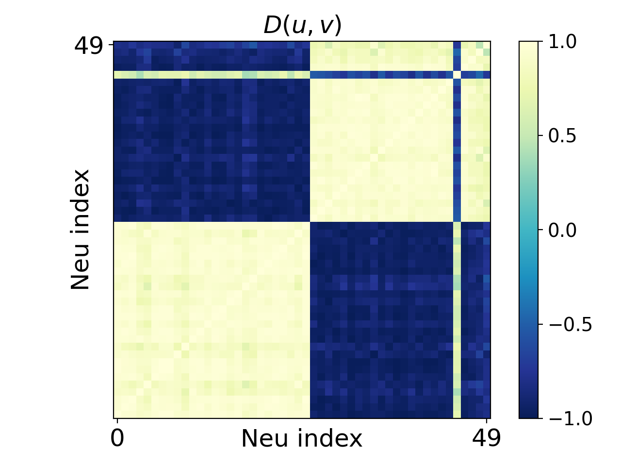
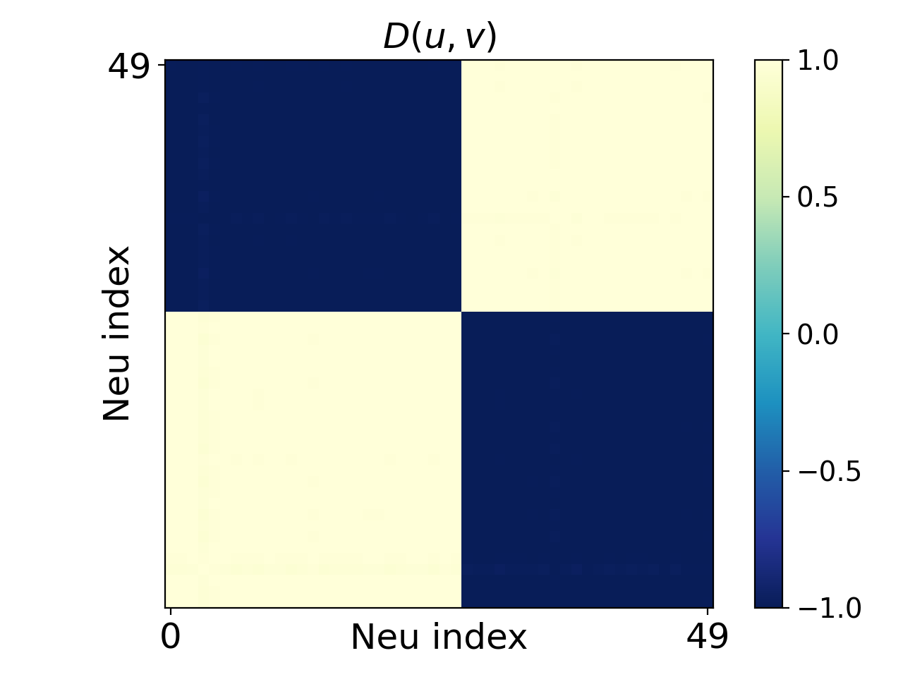
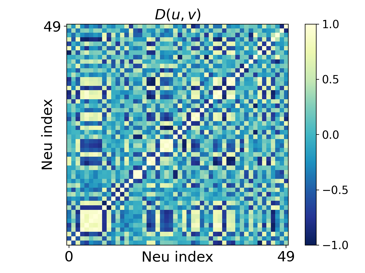
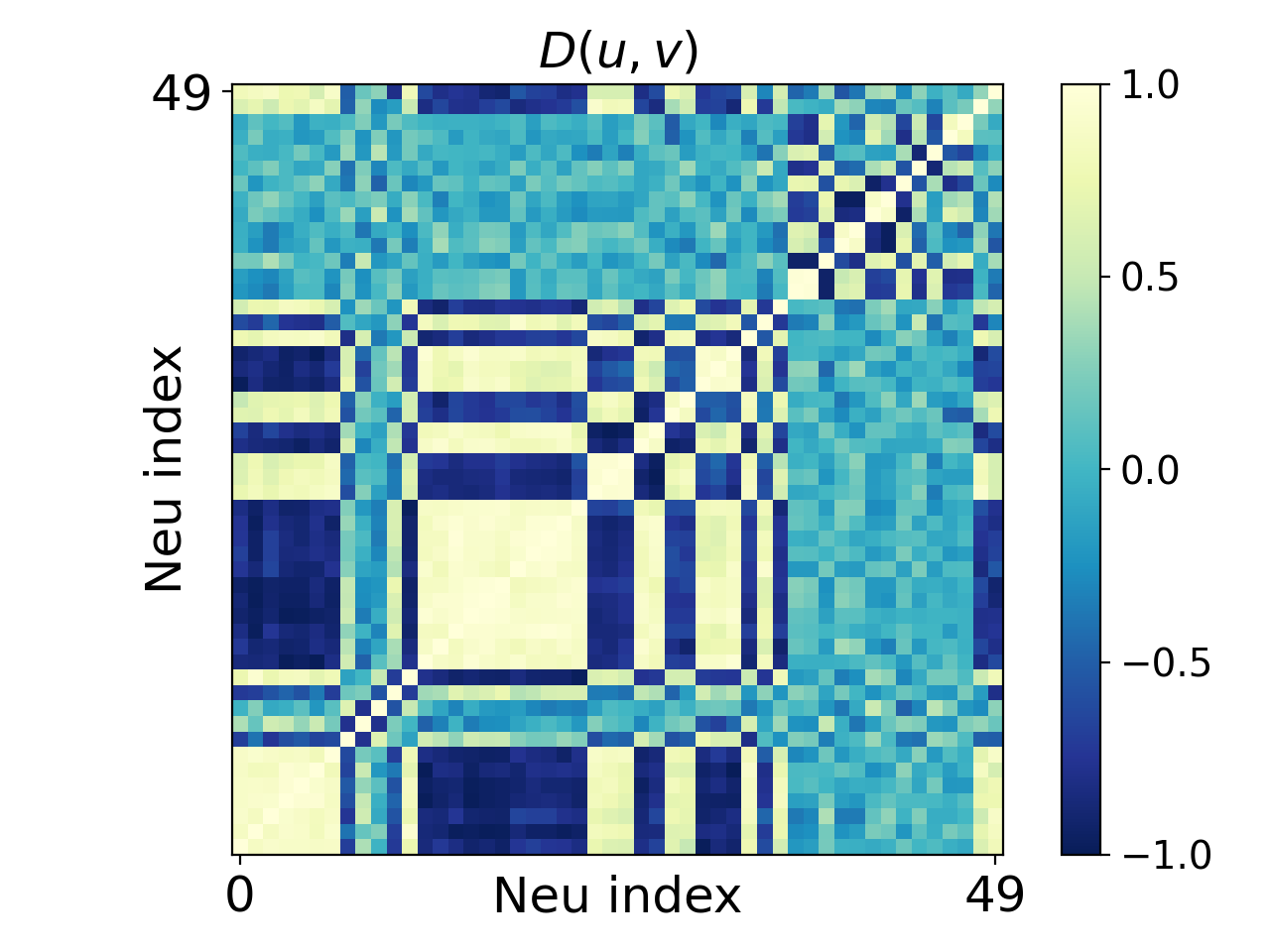
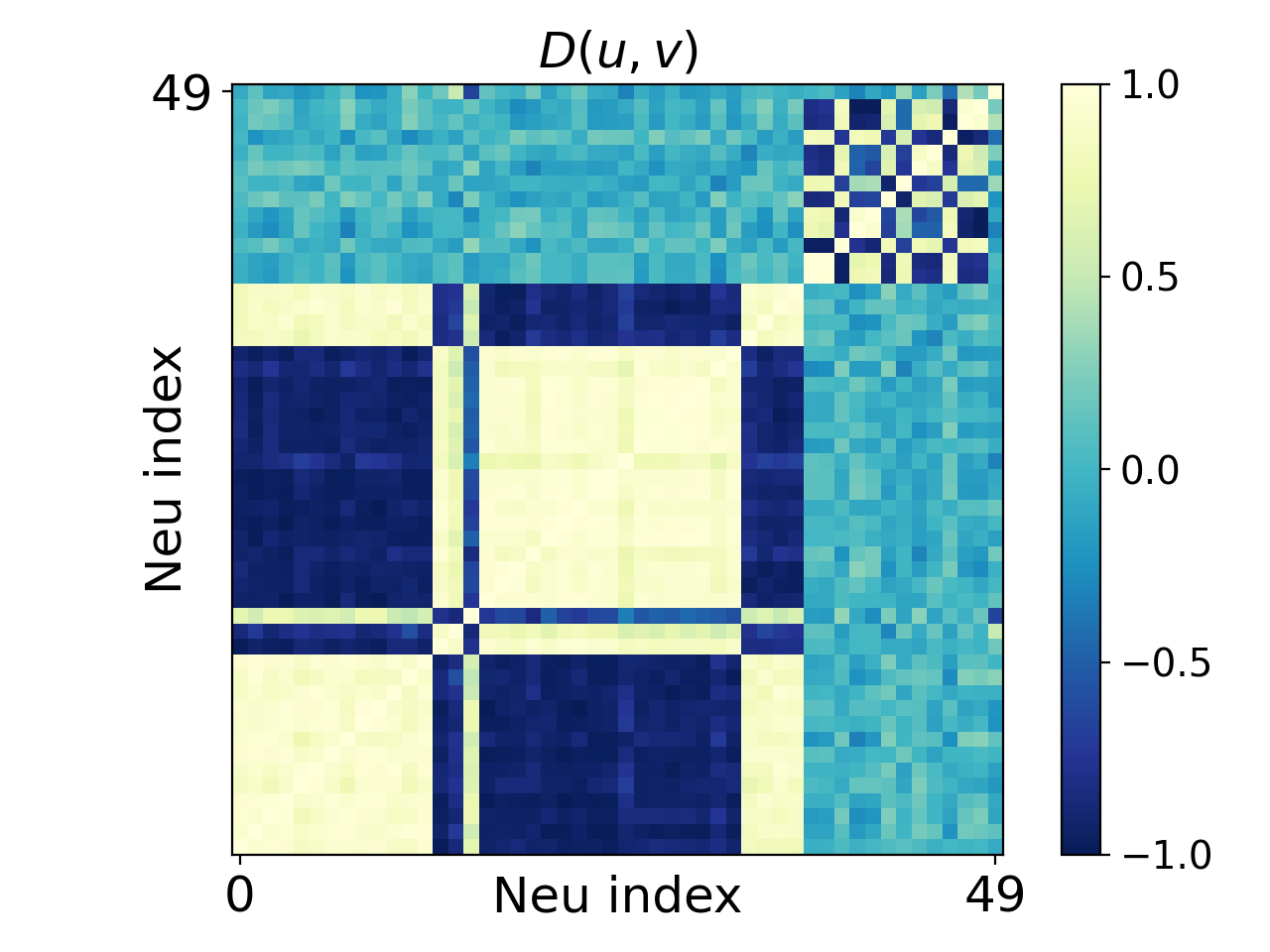
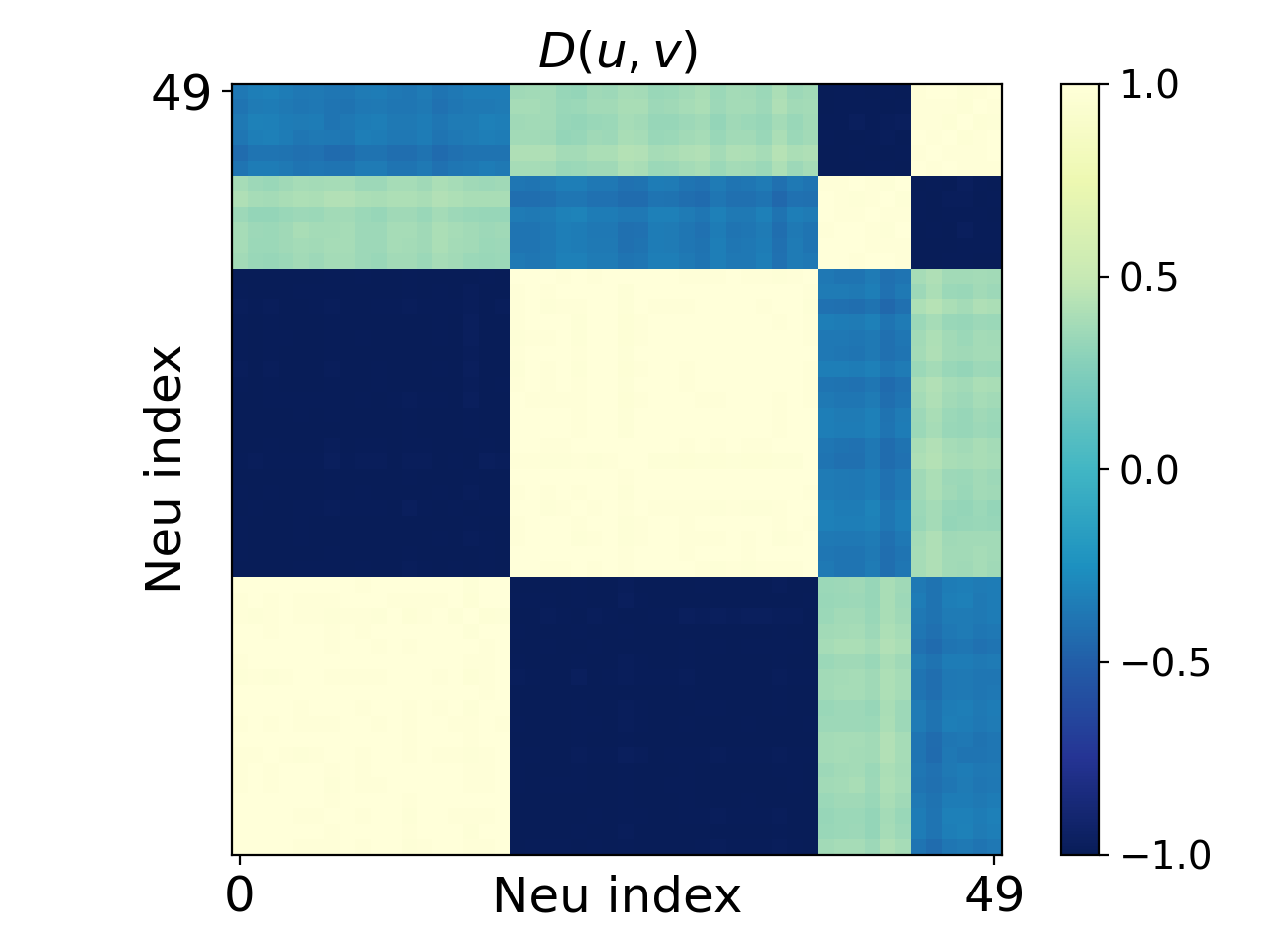
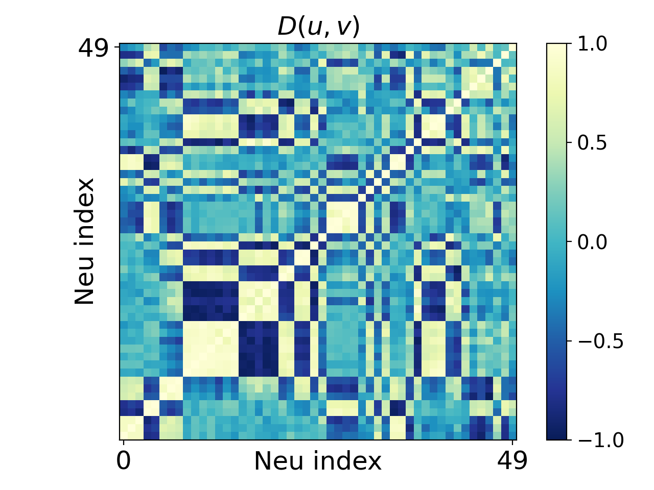
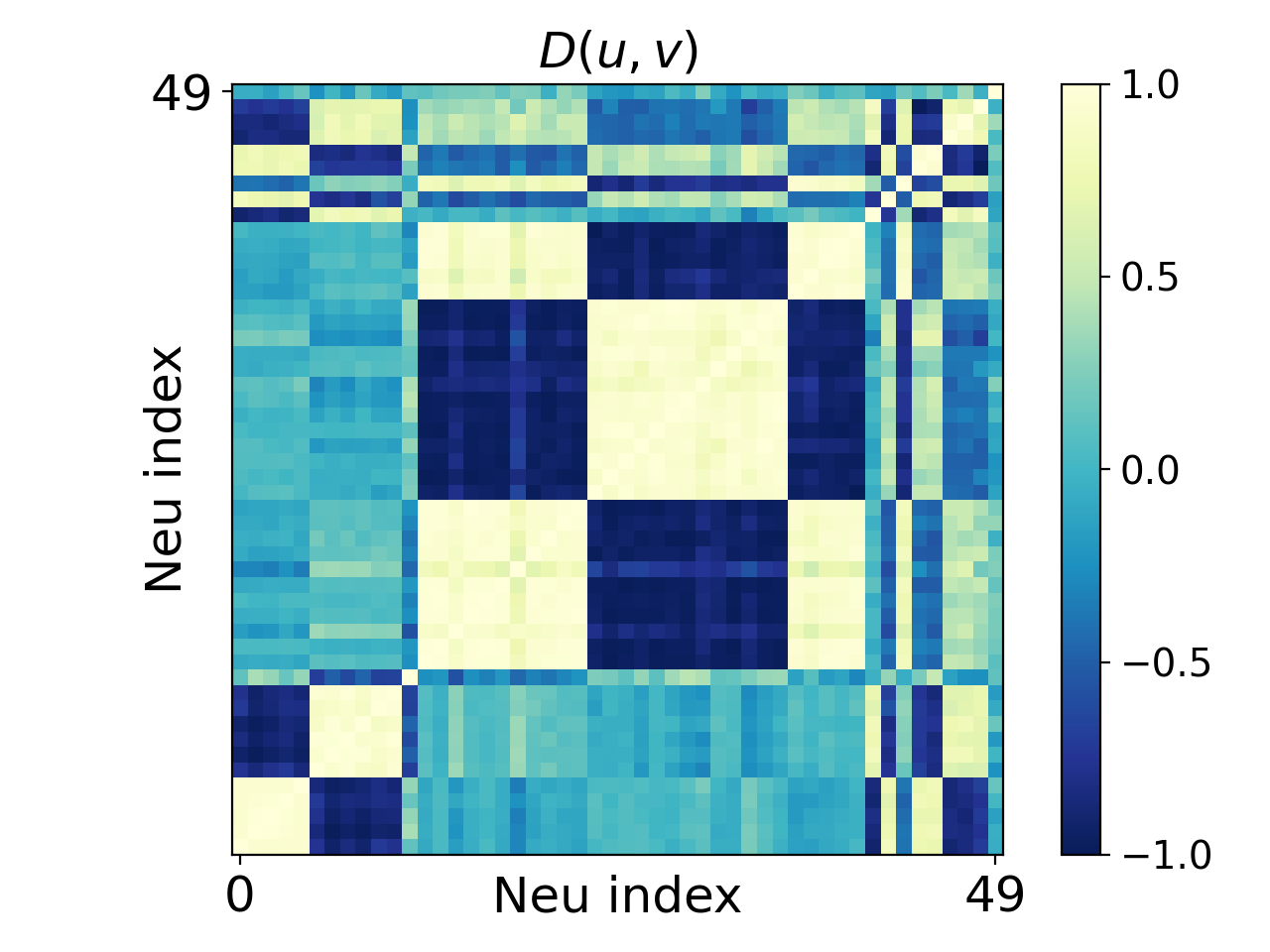
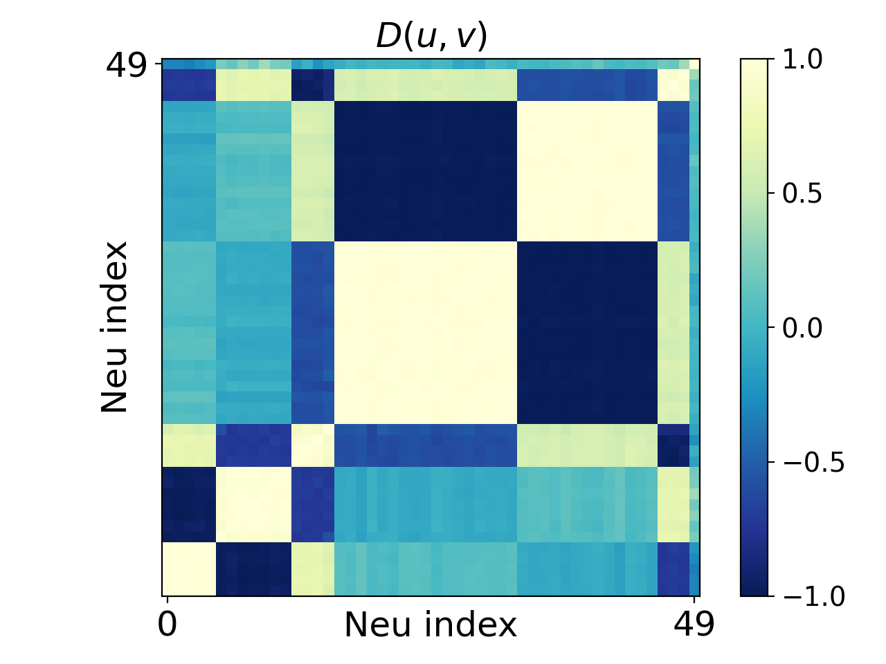
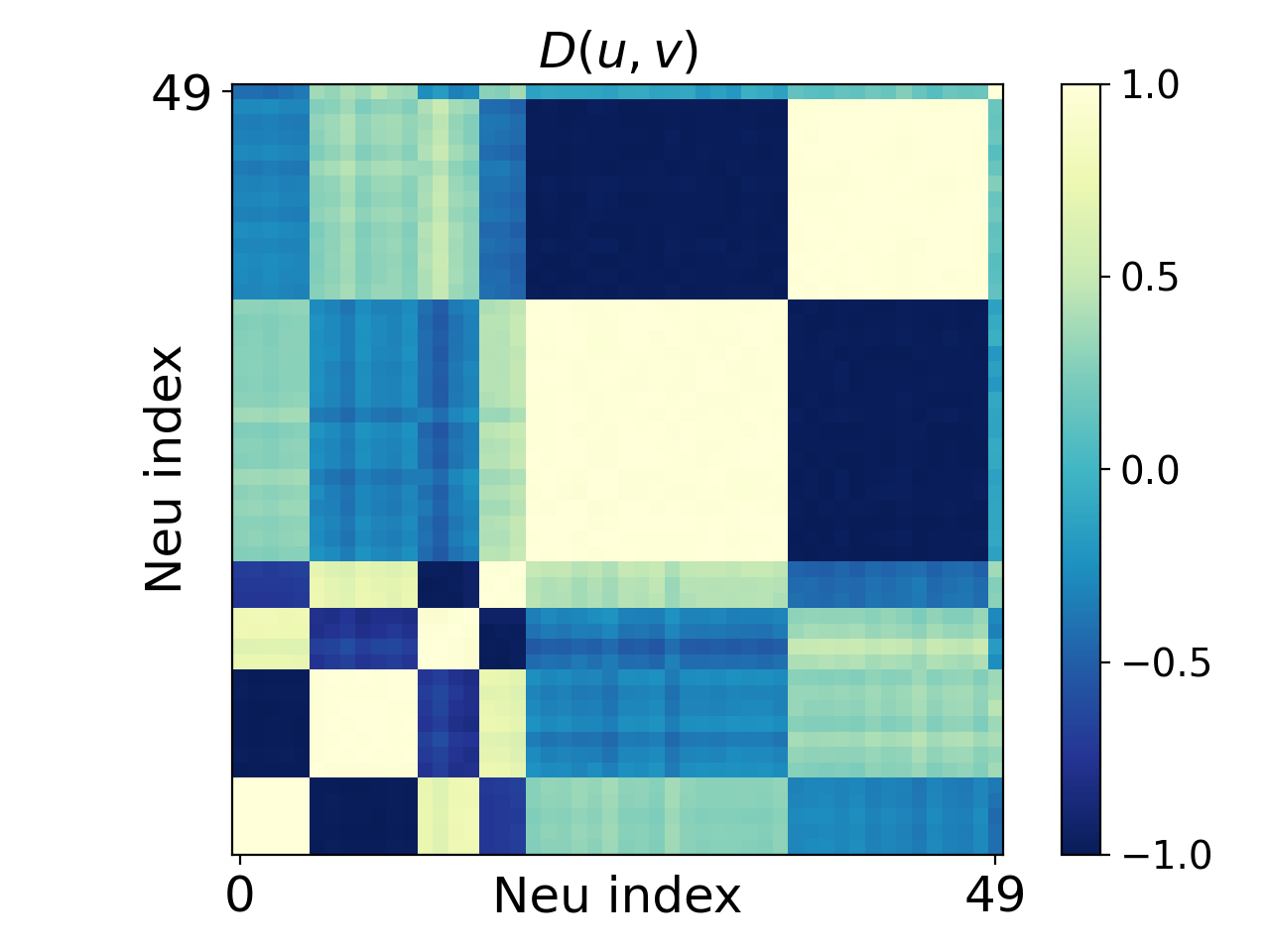
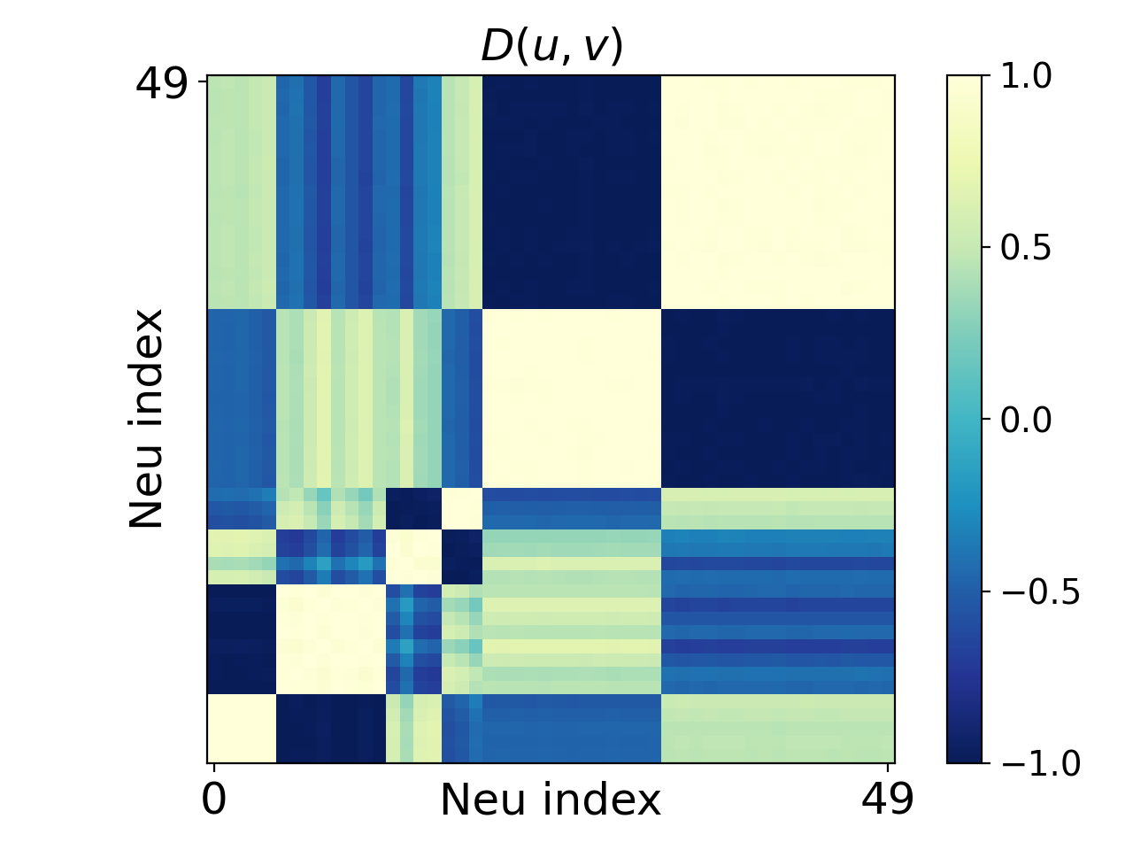
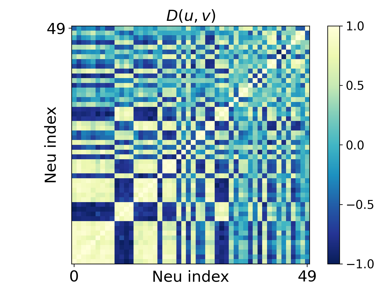
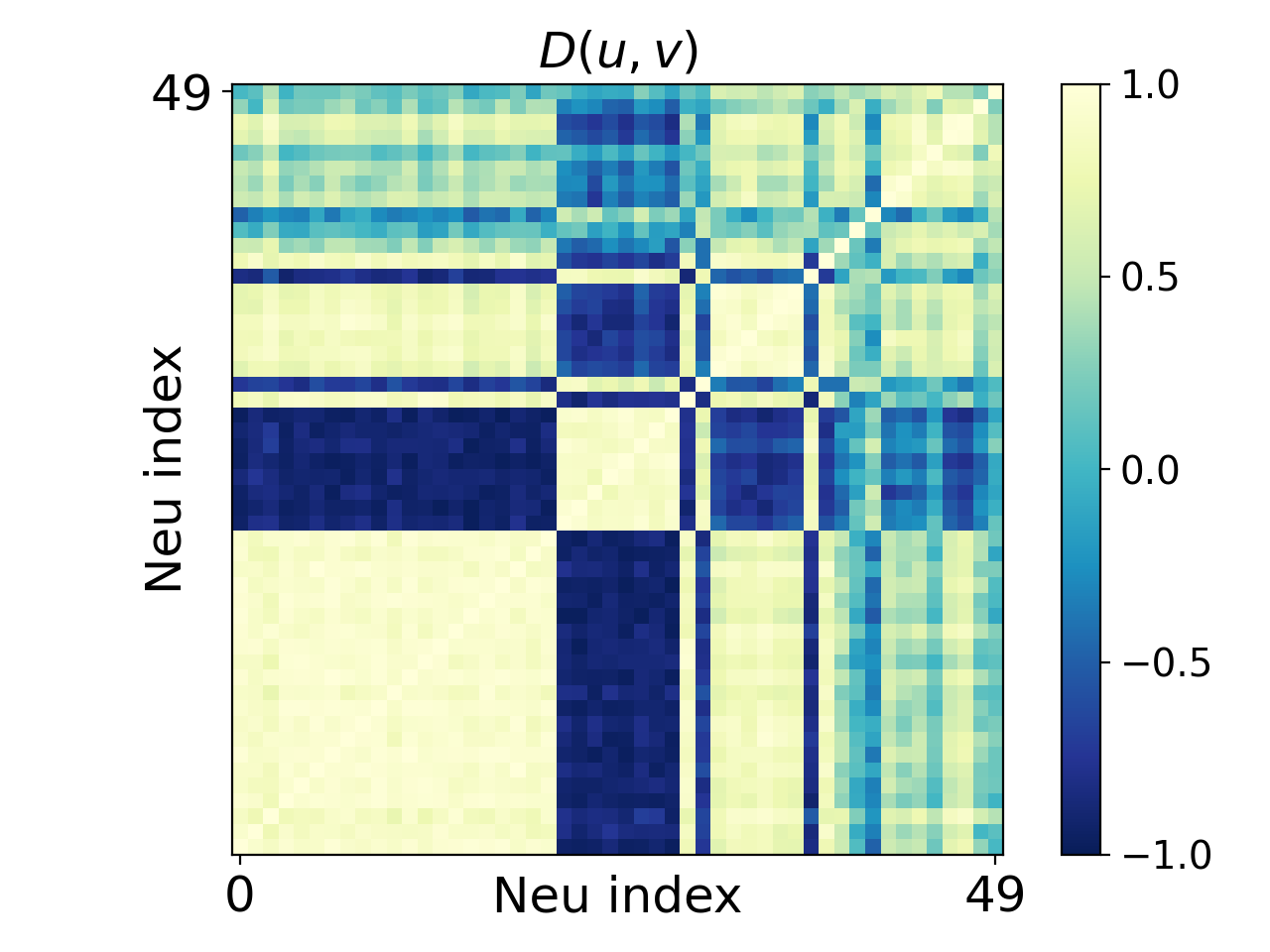
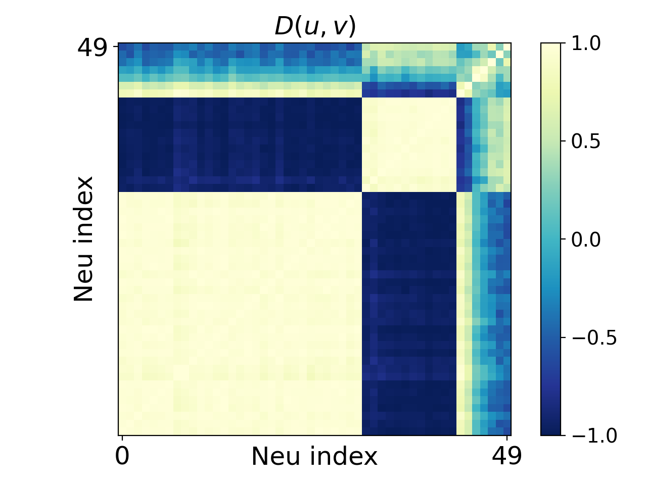
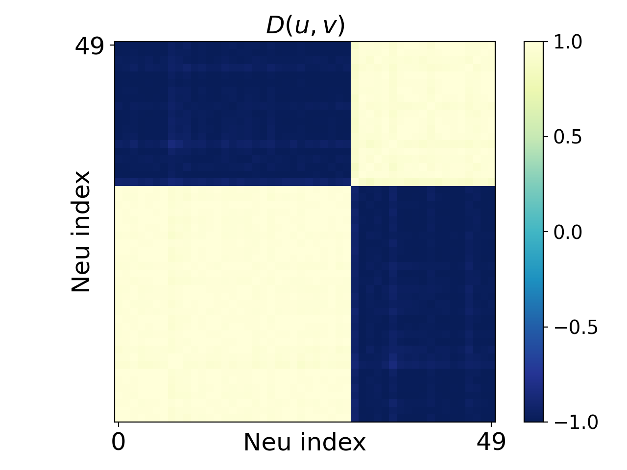
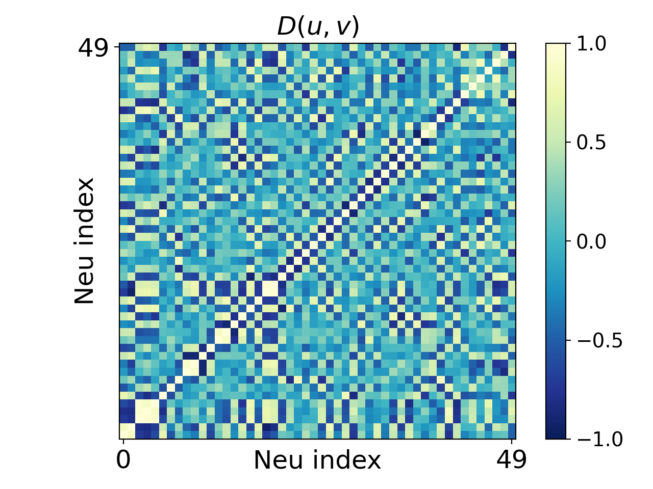
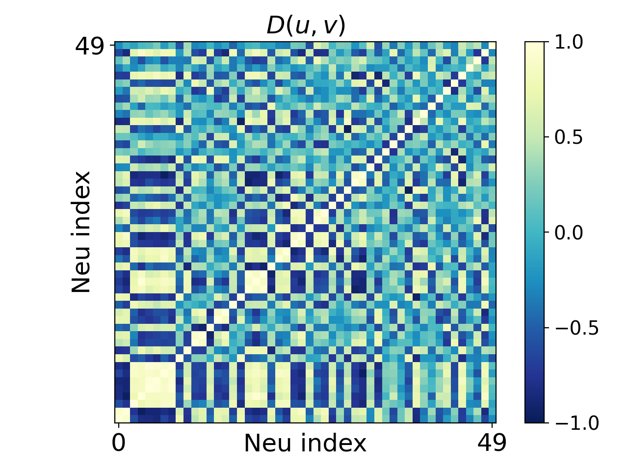
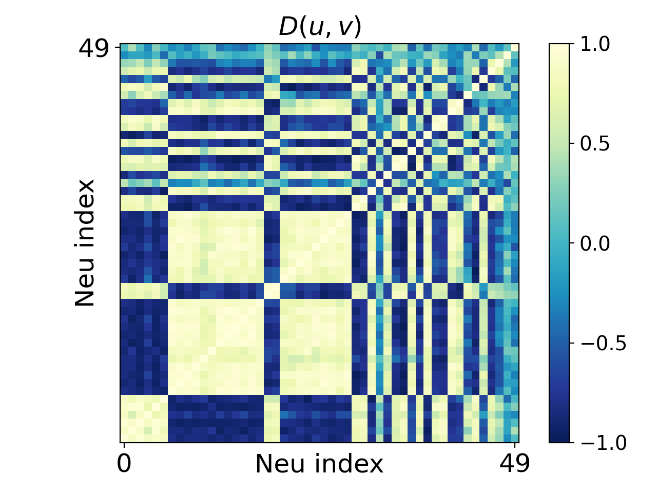
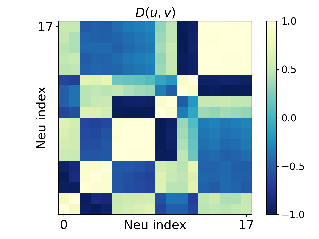
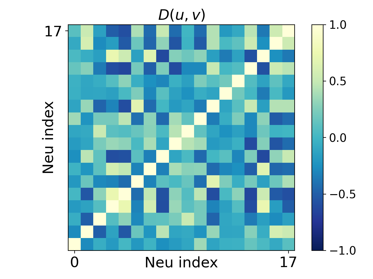
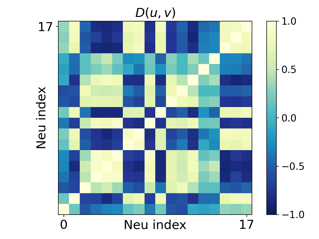
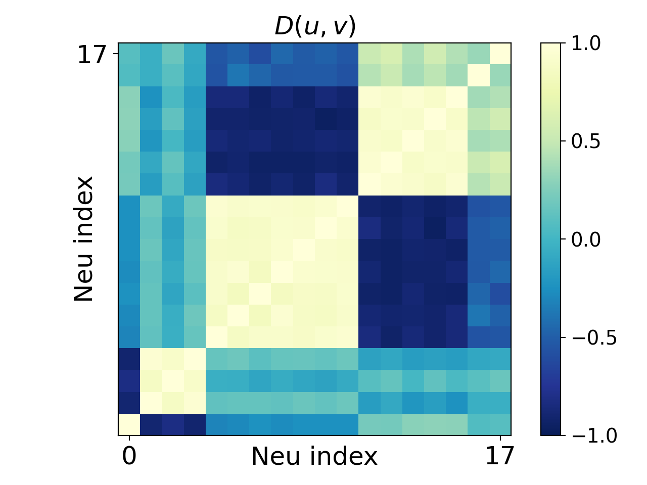
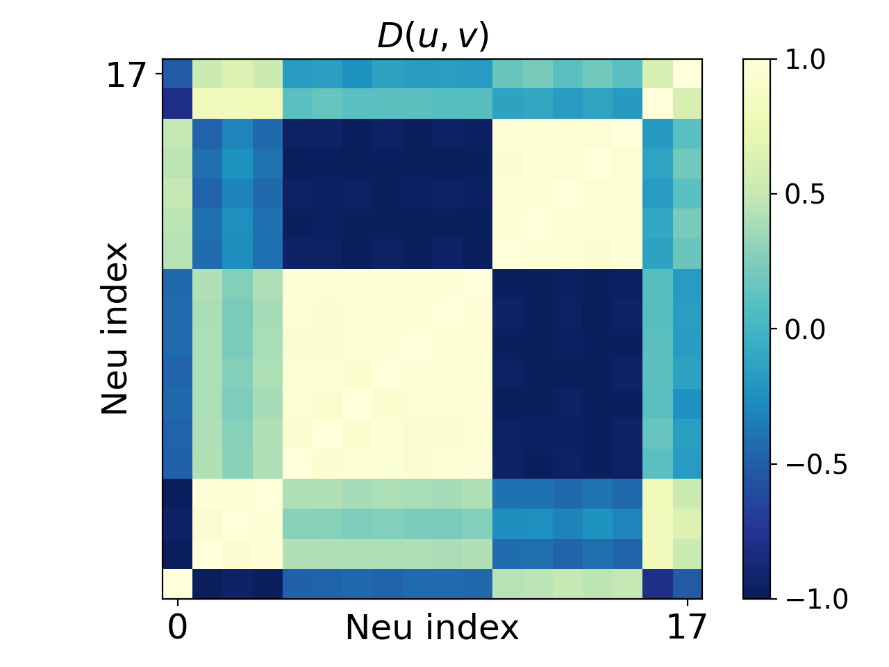
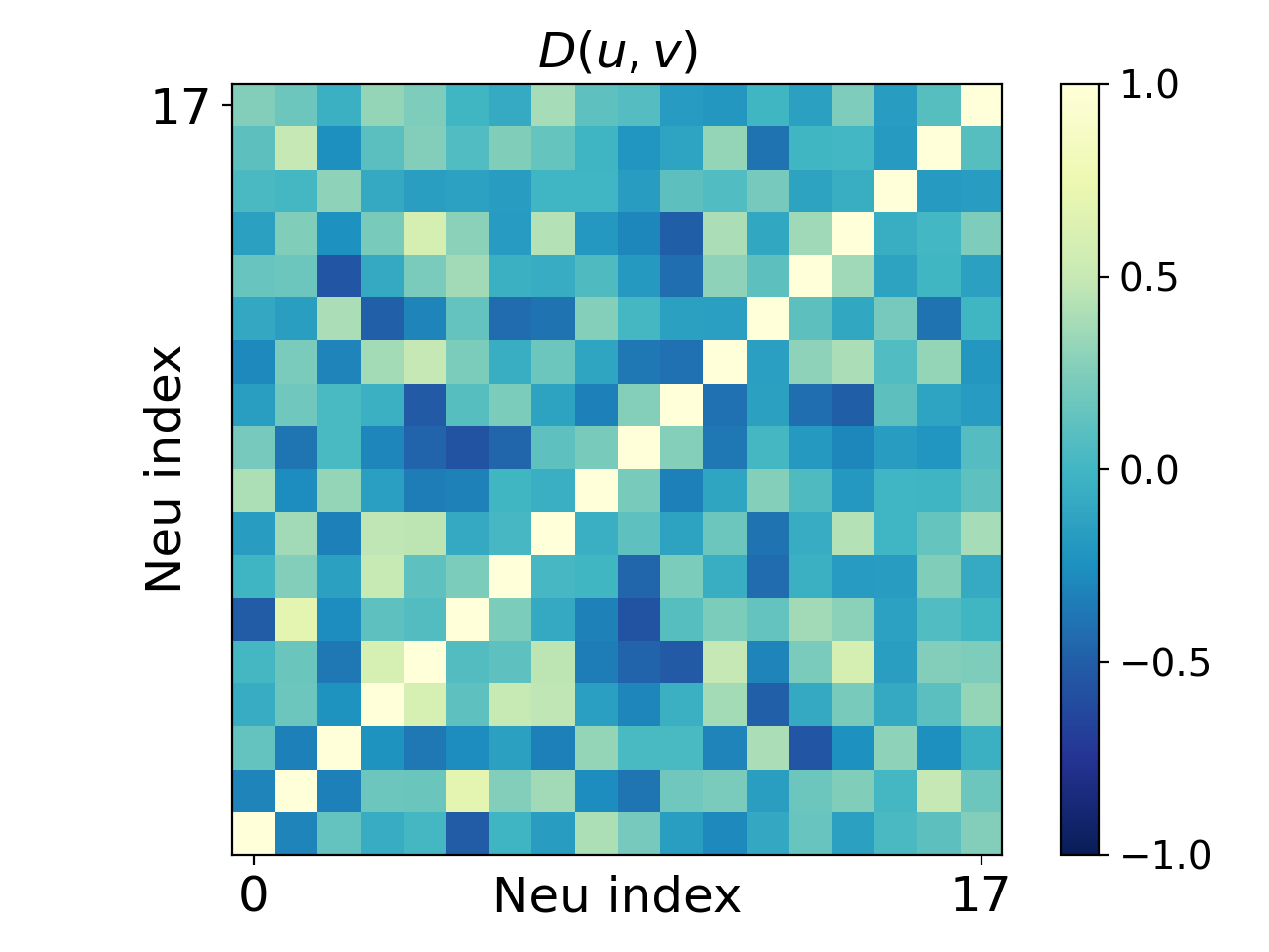
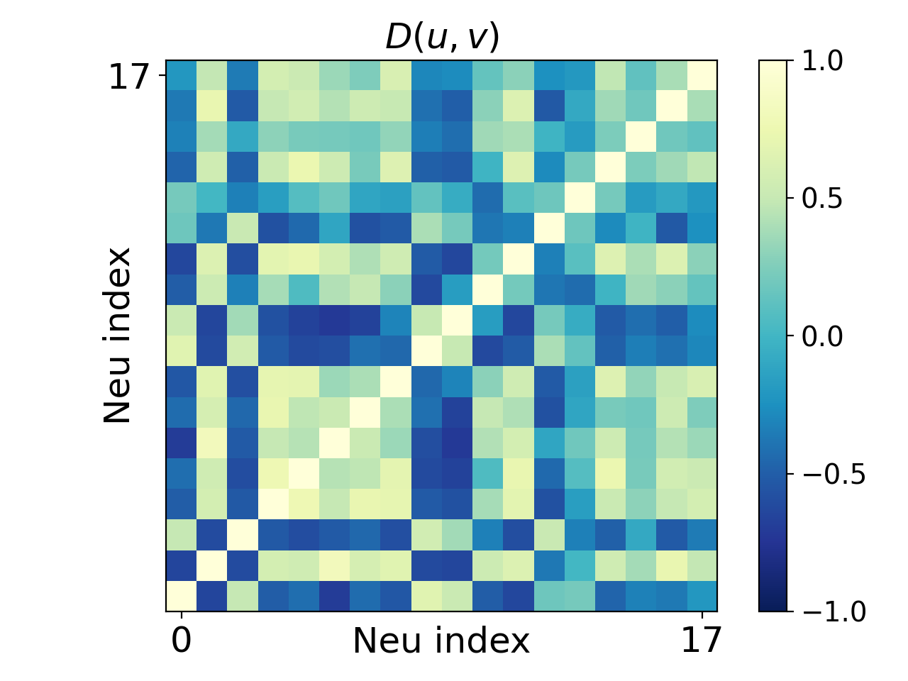
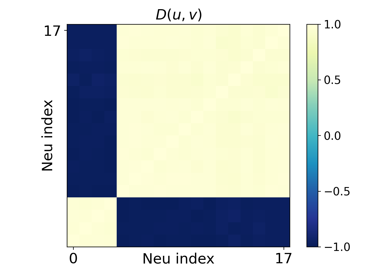
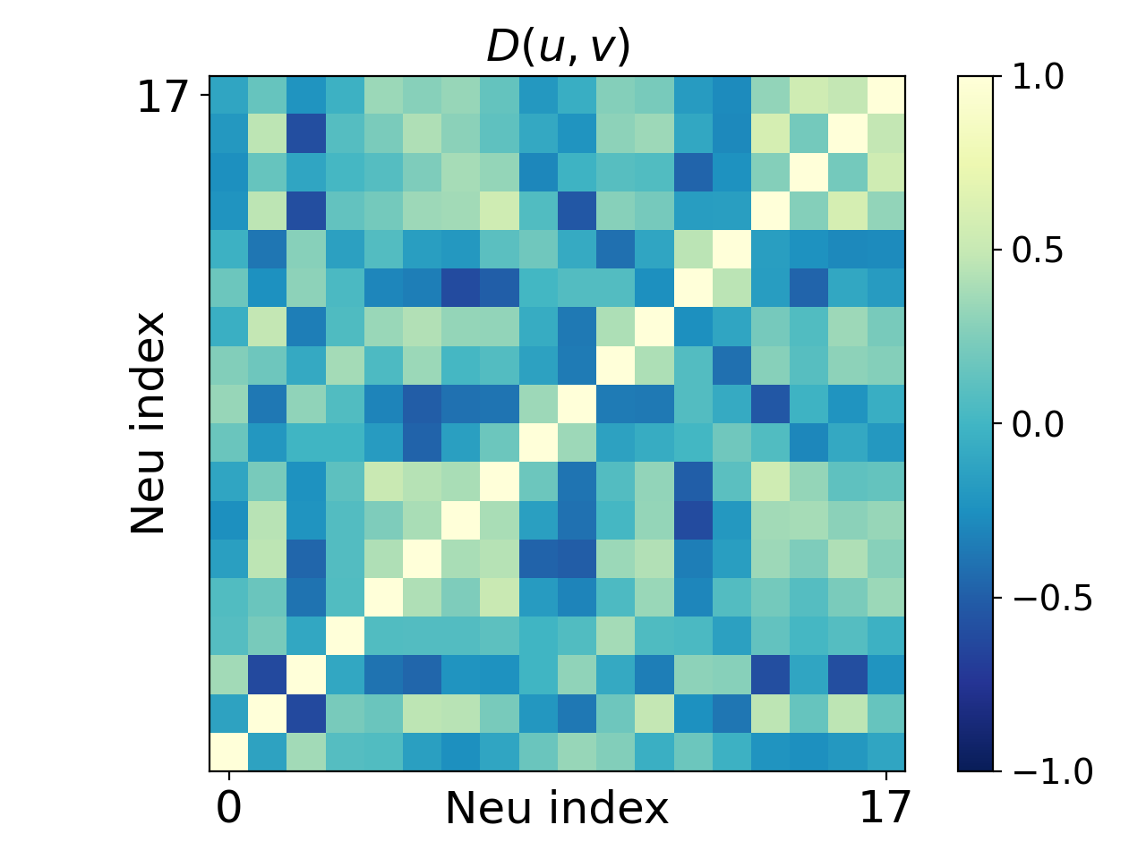
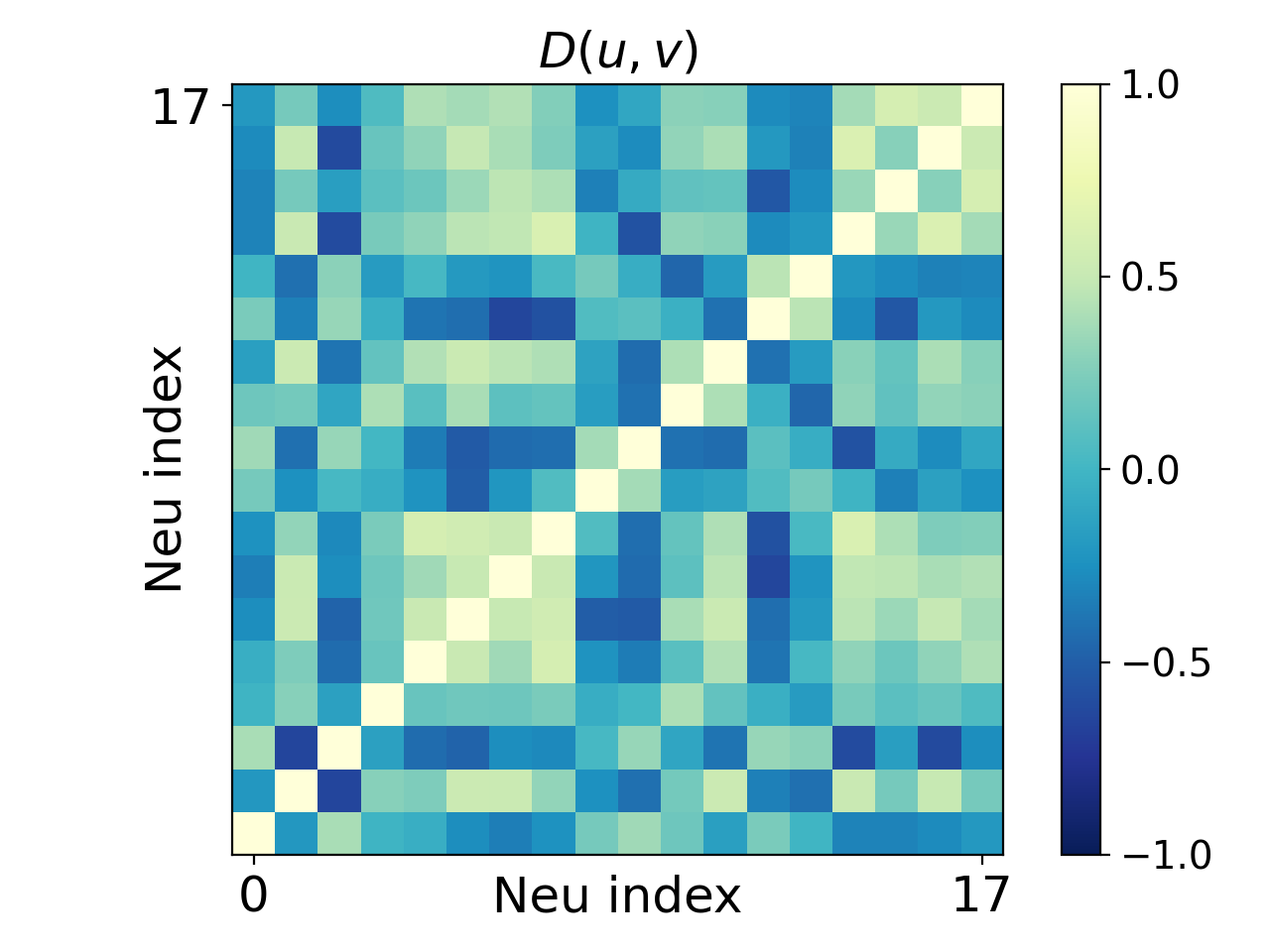
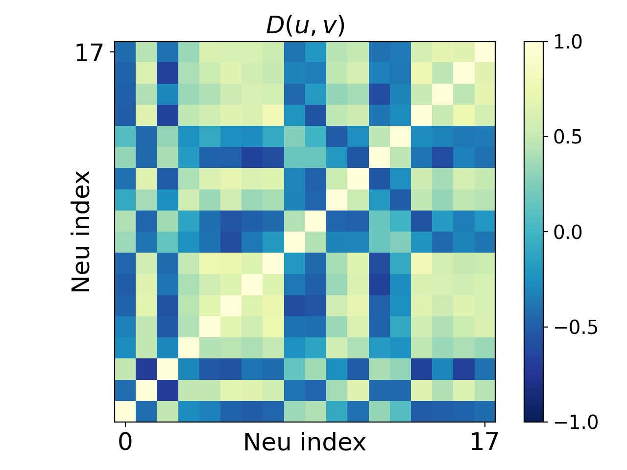
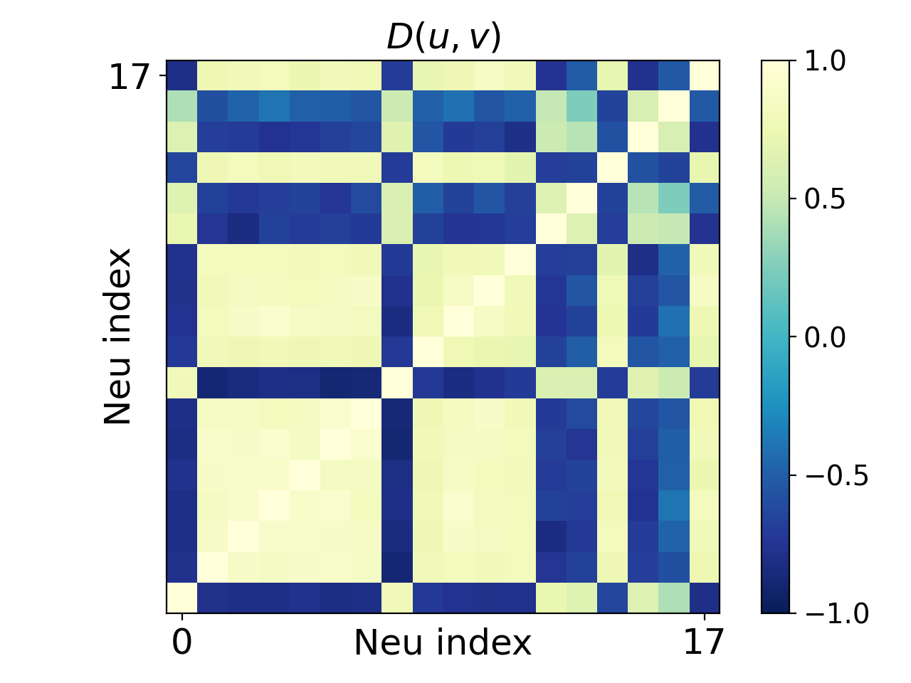
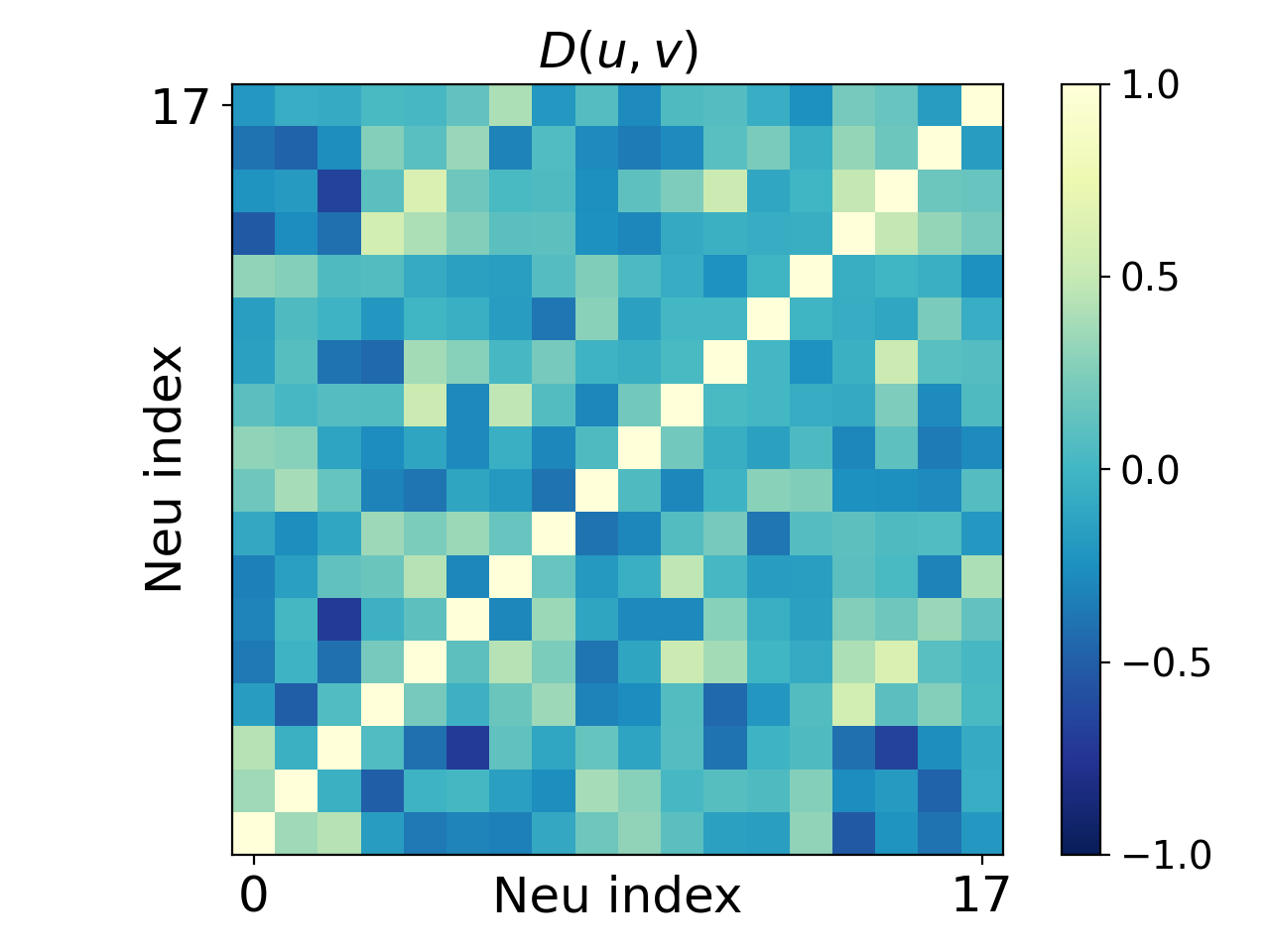
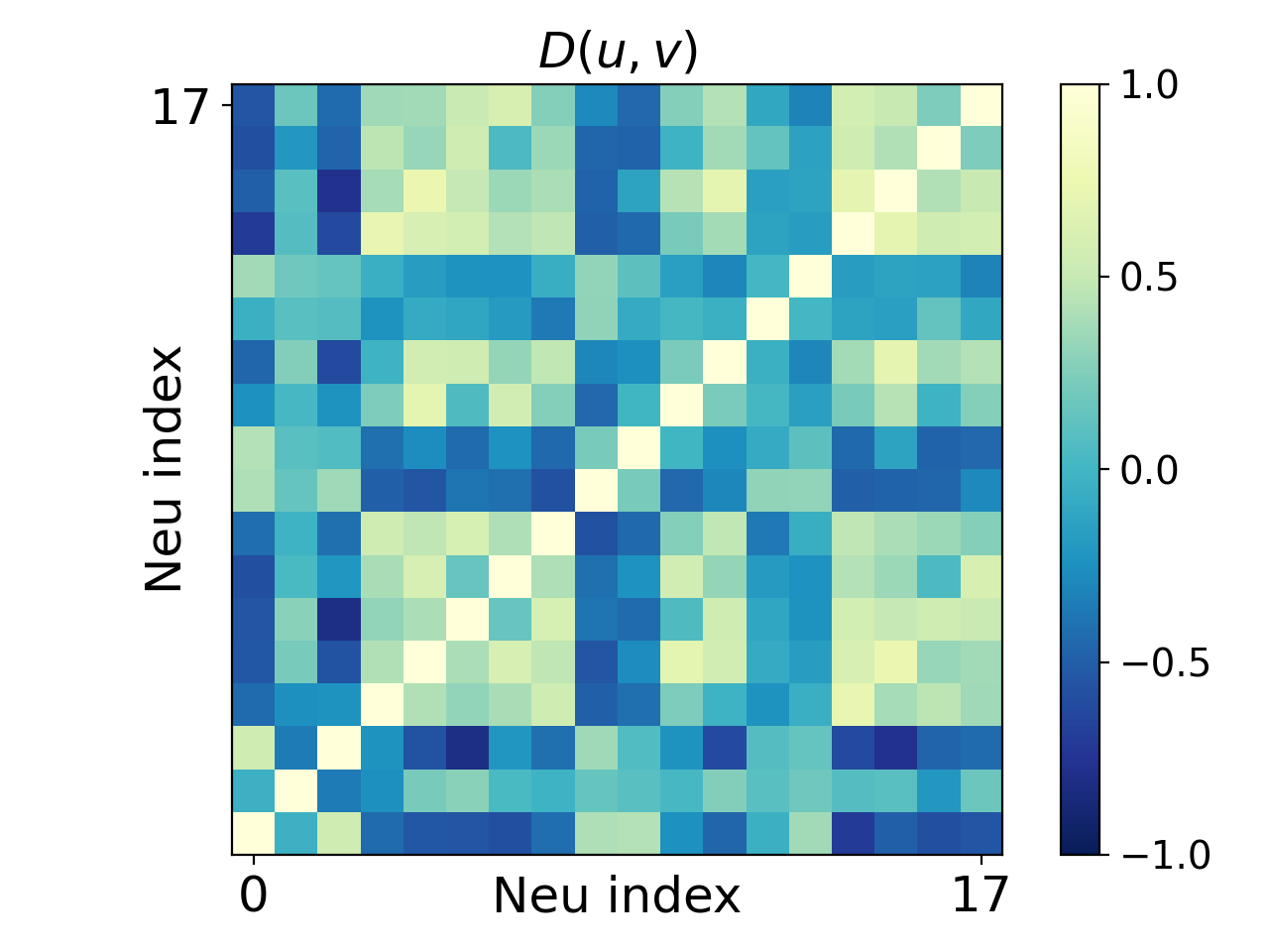
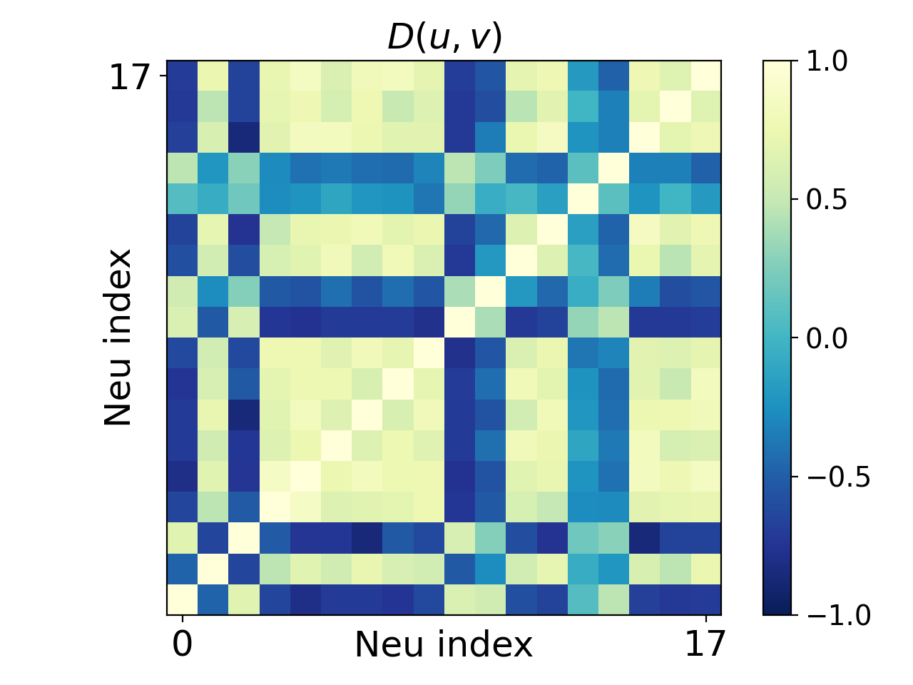
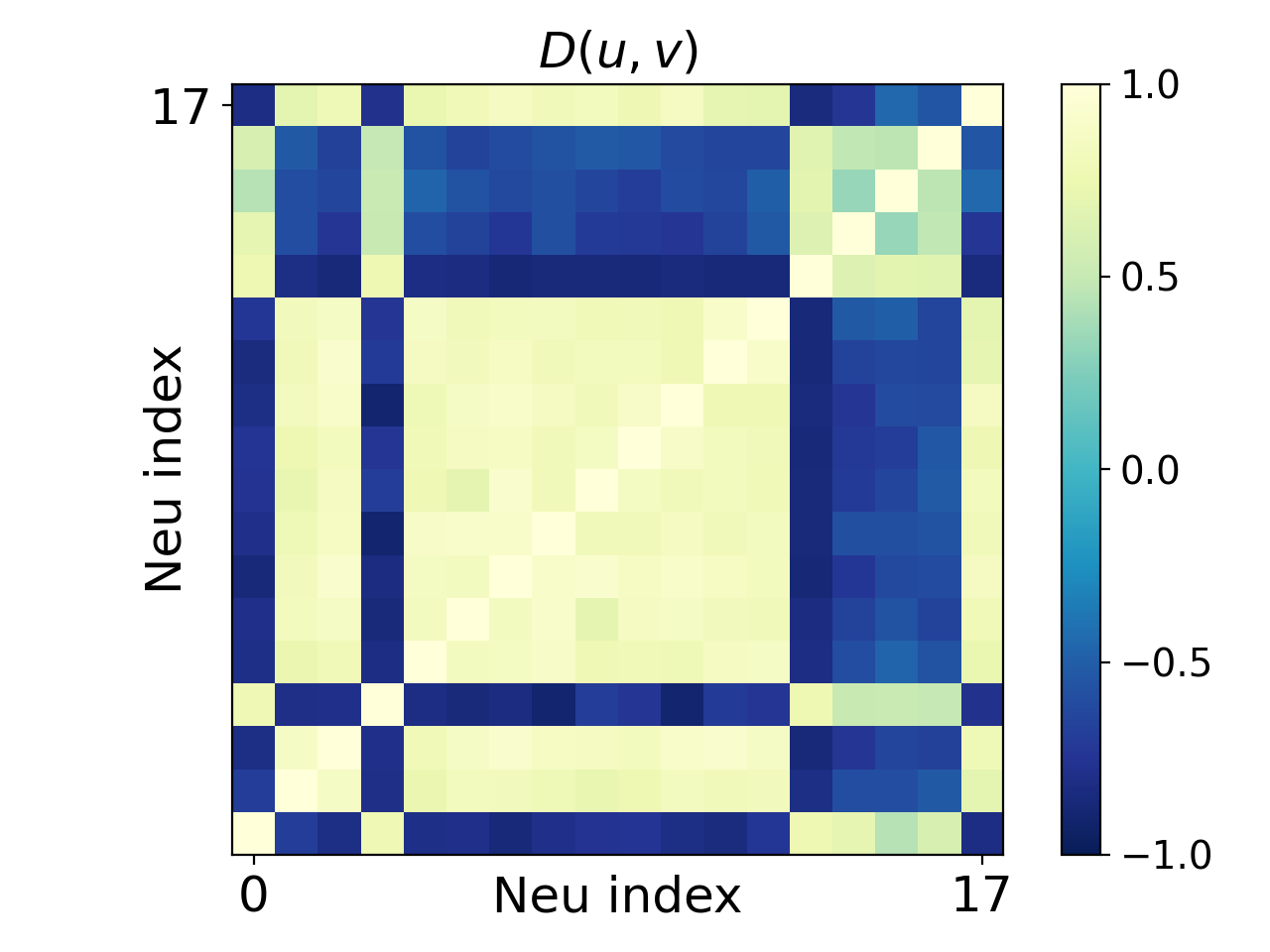
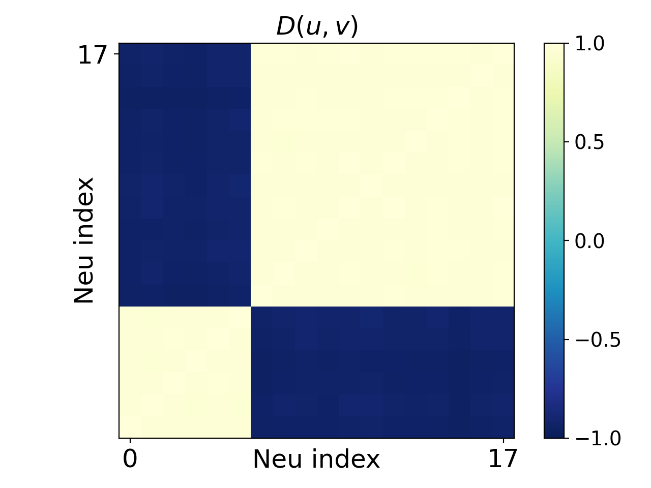
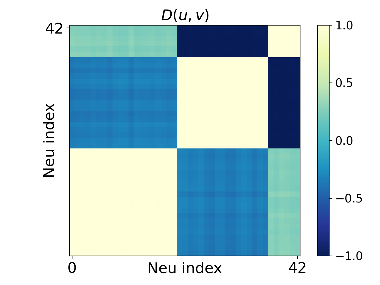
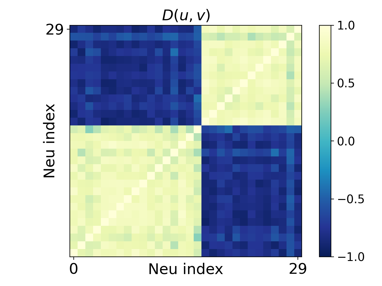
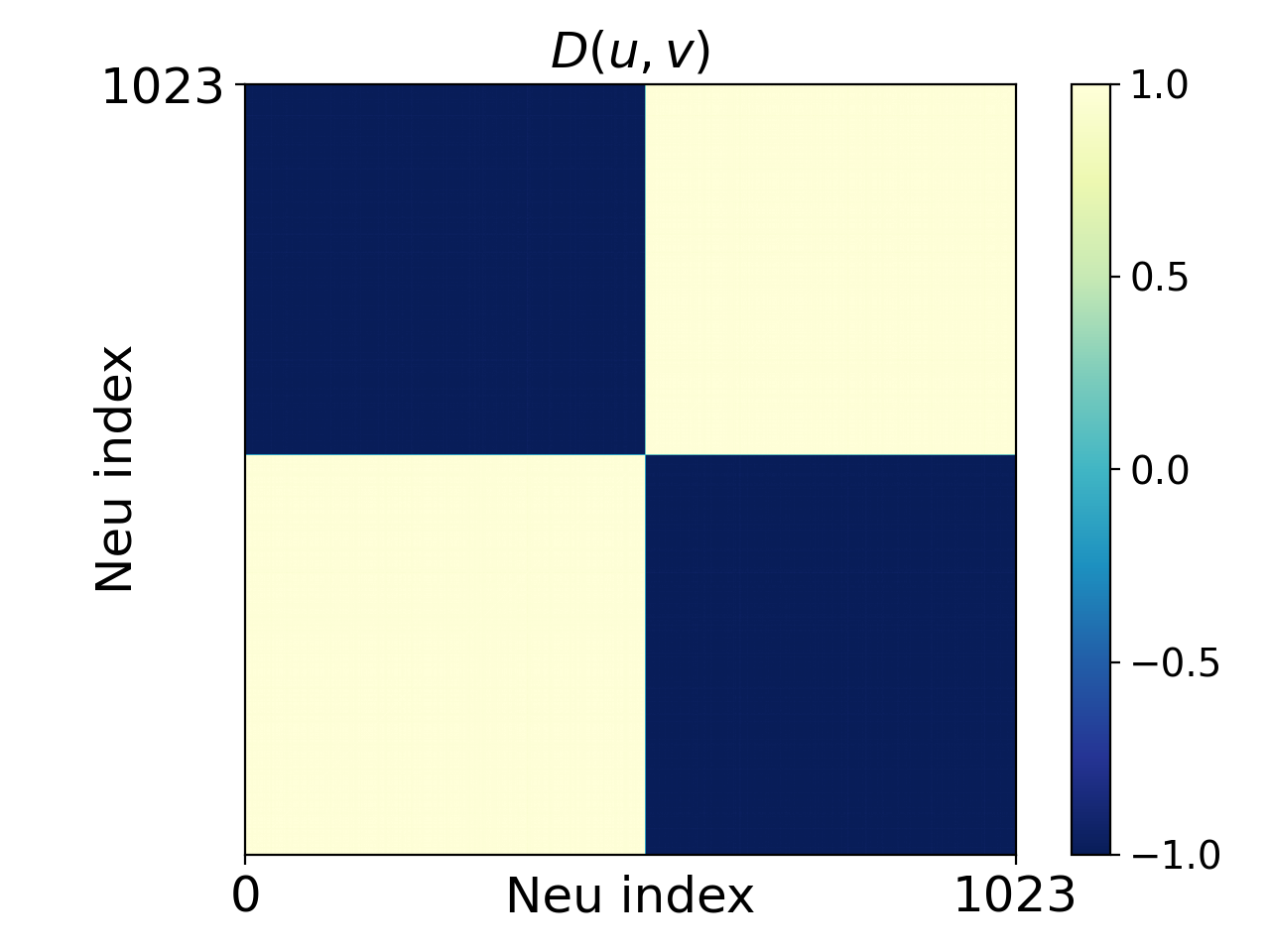
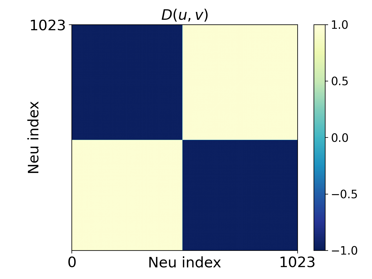
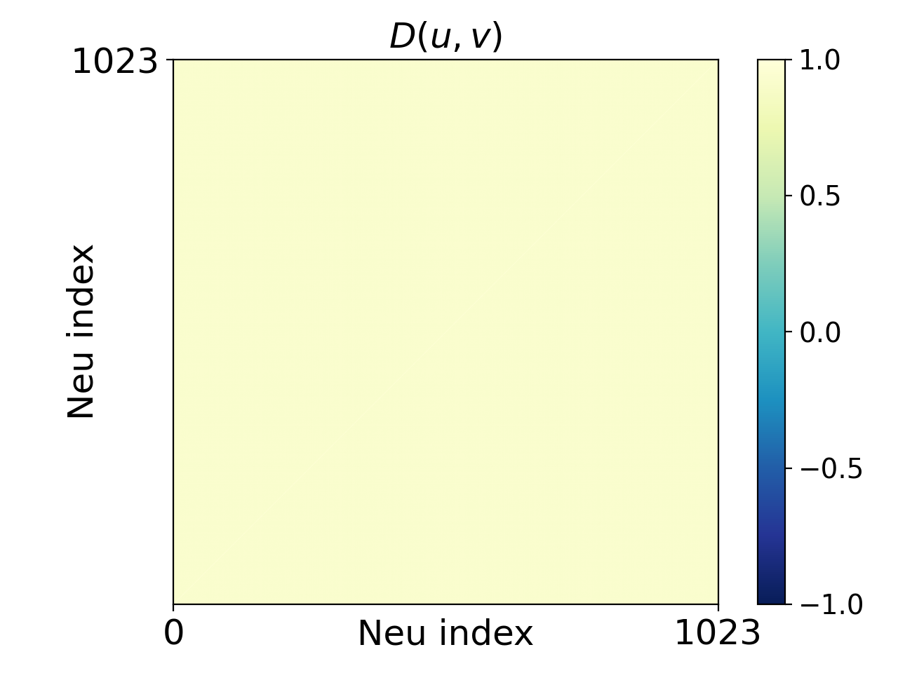
The condensation of the weights of between the fully-connected (FC) layers of a Resnet18-like neural network on CIFAR10 is shown in Fig. 2, whose activation functions for FC layers are tanh(x)𝑥\tanh(x), sigmoid(x)sigmoid𝑥\mathrm{sigmoid}(x), softplus(x)softplus𝑥\mathrm{softplus}(x) and xtanh(x)𝑥𝑥x\tanh(x), indicated by the corresponding sub-captions, respectively. As shown in Fig. 2(a), for activation function tanh(x)𝑥\tanh(x), the color indicates cosine similarity D(𝒖,𝒗)𝐷𝒖𝒗D(\bm{u},\bm{v}) of two hidden neurons’ weights, whose indexes are indicated by the abscissa and the ordinate, respectively. If the neurons are in the same beige block, D(𝒖,𝒗)1similar-to𝐷𝒖𝒗1D(\bm{u},\bm{v})\sim 1 (navy-blue block, D(𝒖,𝒗)1similar-to𝐷𝒖𝒗1D(\bm{u},\bm{v})\sim-1), their input weights have the same (opposite) direction. Input weights of hidden neurons in Fig. 2(a) condense at two opposite directions, i.e., one line. Similarly, weights of hidden neurons for NNs with sigmoid(x)sigmoid𝑥\mathrm{sigmoid}(x) and softplus(x)softplus𝑥\mathrm{softplus}(x) (Fig. 2(b, c)), which are frequently used and have multiplicity one, condense at one direction. As the multiplicity increases, NNs with xtanhx𝑥𝑥x\tanh{x} (Fig. 2(d)) condense at two different lines. These experiments suggest that the condensation is closely related to the multiplicity of the activation function.

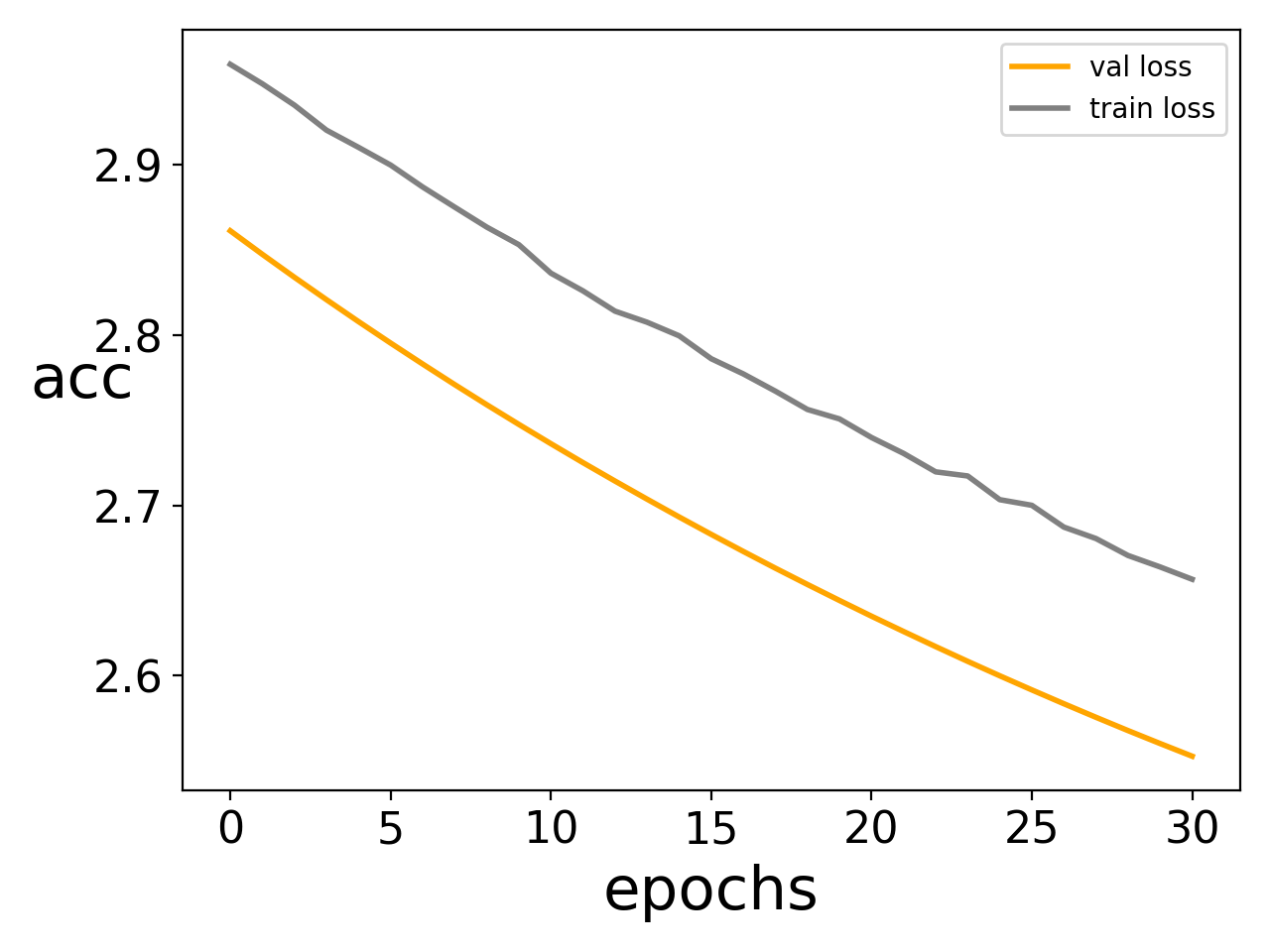
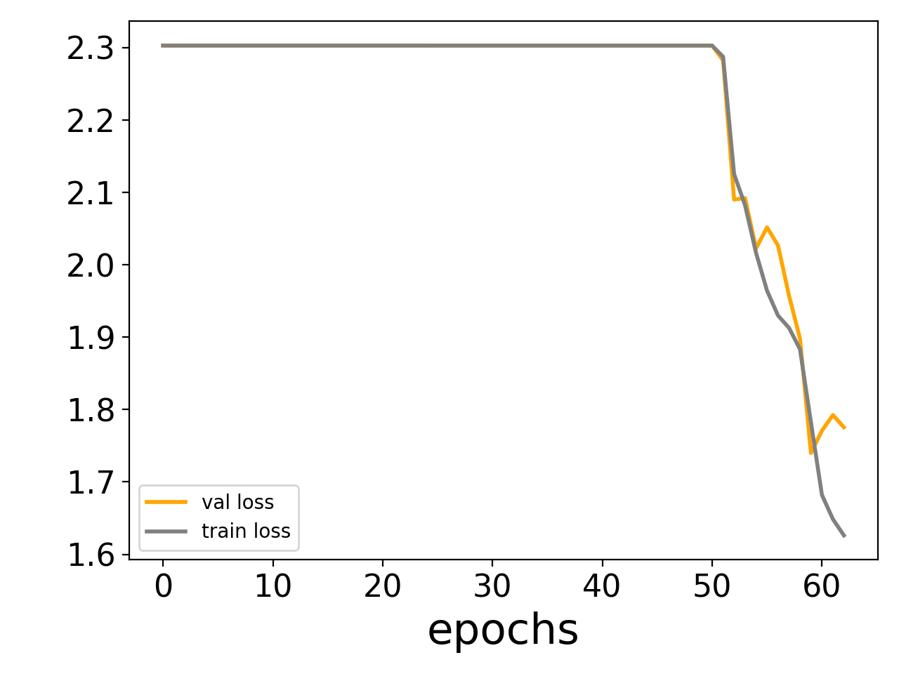
In these experiments, we find that the performance of the Resnet18-like network with tanh FC layers with small initialization is similar to the one with common initialization in Appendix A.4.
Refer to caption
(a) tanh(x)𝑥\tanh(x)
Refer to caption
(b) sigmoid(x)sigmoid𝑥\mathrm{sigmoid}(x)
Refer to caption
(c) softplus(x)softplus𝑥\mathrm{softplus}(x)
Refer to caption
(d) xtanh(x)𝑥𝑥x\tanh(x)
Figure 2: Condensation of Resnet18-like neural networks on CIFAR10. Each network consists of the convolution part of resnet18 and fully-connected (FC) layers with size 1024-1024-10 and softmax. The color in figures indicates the cosine similarity of normalized input weights of two neurons in the first FC layer, whose indexes are indicated by the abscissa and the ordinate, respectively. The convolution part is equipped with ReLU activation and initialized by Glorot normal distribution (Glorot and Bengio, 2010). The activation functions are tanh(x)𝑥\tanh(x), sigmoid(x)sigmoid𝑥\mathrm{sigmoid}(x), softplus(x)softplus𝑥\mathrm{softplus}(x) and xtanh(x)𝑥𝑥x\tanh(x) for FC layers in (a), (b), (c), and (d), separately. The numbers of steps selected in the sub-pictures are epoch 20, epoch 30, epoch 30 and epoch 61, respectively. The learning rate is 3×1083superscript1083\times 10^{-8}, 1×1081superscript1081\times 10^{-8}, 1×1081superscript1081\times 10^{-8} and 5×1065superscript1065\times 10^{-6}, separately .The FC layers are initialized by N(0,1mout3)𝑁01superscriptsubscript𝑚out3N(0,\frac{1}{m_{\rm out}^{3}}), and Adam optimizer with cross-entropy loss and batch size 128 are used for all experiments.

4.3 Multidimensional synthetic data

Refer to caption
(a) tanh(x)𝑥\tanh(x)
Refer to caption
(b) xtanh(x)𝑥𝑥x\tanh(x)
Refer to caption
(c) x2tanh(x)superscript𝑥2𝑥x^{2}\tanh(x)
Refer to caption
(d) sigmoid(x)sigmoid𝑥\mathrm{sigmoid}(x)
Refer to caption
(e) softplus(x)softplus𝑥\mathrm{softplus}(x)
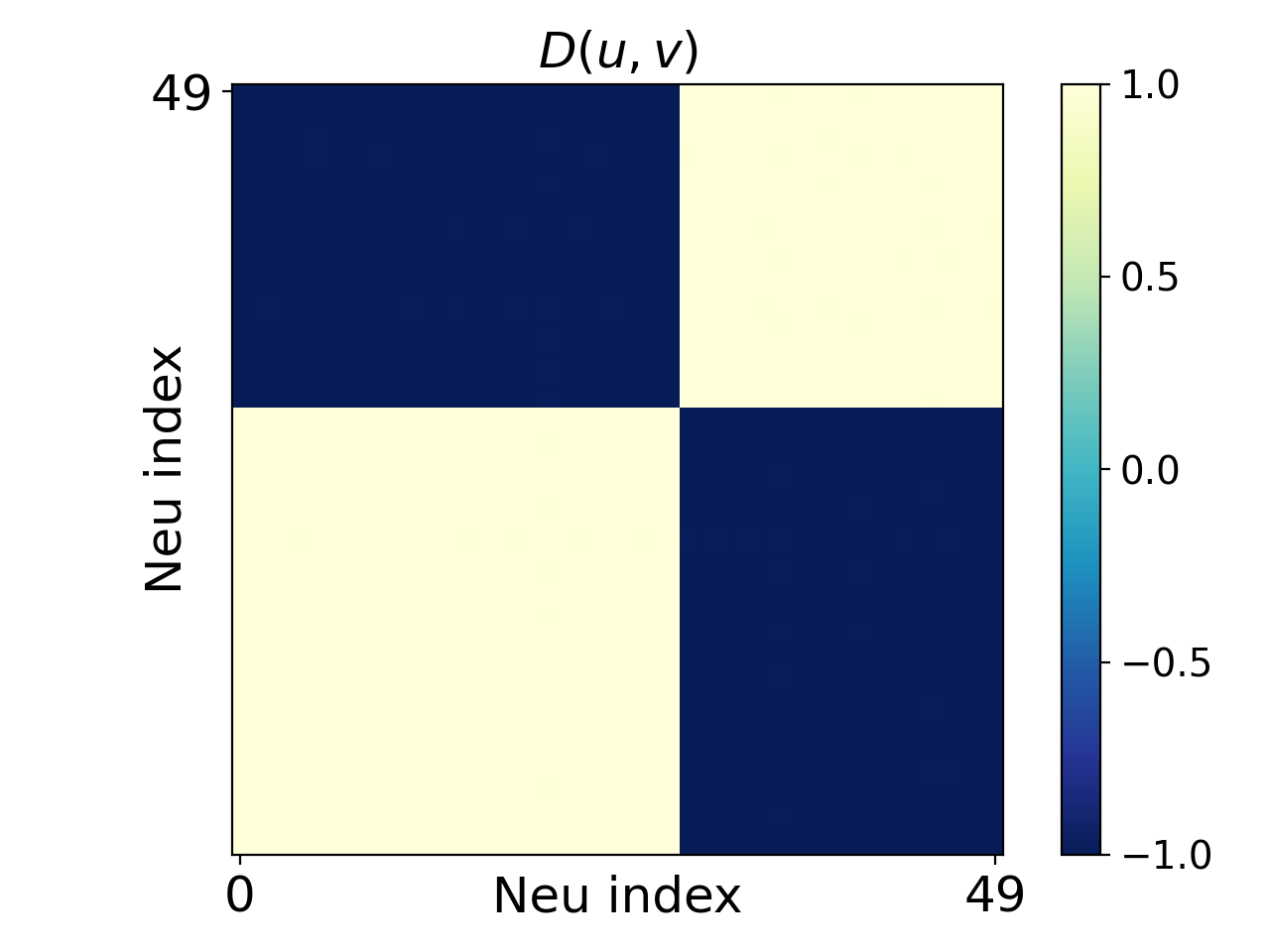
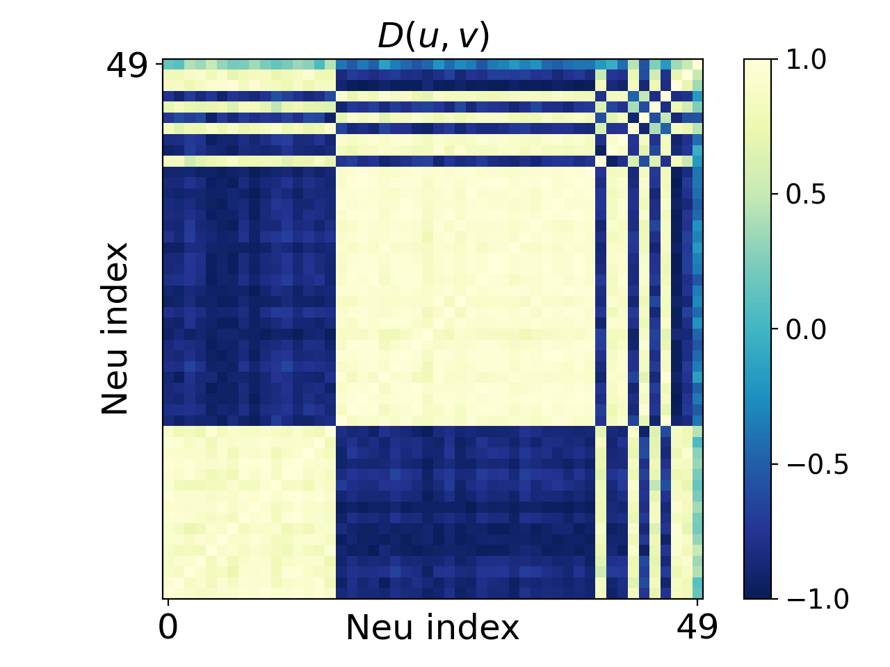
Figure 3: Condensation of two-layer NNs. The color indicates D(𝒖,𝒗)𝐷𝒖𝒗D(\bm{u},\bm{v}) of two hidden neurons’ input weights at epoch 100100100, whose indexes are indicated by the abscissa and the ordinate, respectively. If neurons are in the same beige block, D(𝒖,𝒗)1similar-to𝐷𝒖𝒗1D(\bm{u},\bm{v})\sim 1 (navy-blue block, D(𝒖,𝒗)1similar-to𝐷𝒖𝒗1D(\bm{u},\bm{v})\sim-1), their input weights have the same (opposite) direction. The activation functions are indicated by the sub-captions. The training data is 808080 points sampled from k=153.5sin(5xk+1)superscriptsubscript𝑘153.55subscript𝑥𝑘1\sum_{k=1}^{5}3.5\sin(5x_{k}+1), where each xksubscript𝑥𝑘x_{k} is uniformly sampled from [4,2]42[-4,2]. n=80𝑛80n=80, d=5𝑑5d=5, m=50𝑚50m=50, dout=1subscript𝑑out1d_{\mathrm{out}}=1, var=0.0052varsuperscript0.0052\mathrm{var}=0.005^{2}. lr=103,8×104,2.5×104lrsuperscript1038superscript1042.5superscript104\mathrm{lr}=10^{-3},8\times 10^{-4},2.5\times 10^{-4} for (a-c), (d) and (e), respectively.

For convenience of experiments, we then use synthetic data to perform extensive experiments to study the relation between the condensation and the multiplicity of the activation function.

We use two-layer fully-connected NNs with size 555-505050-111 to fit n=80𝑛80n=80 training data sampled from a 5-dimensional function k=153.5sin(5xk+1)superscriptsubscript𝑘153.55subscript𝑥𝑘1\sum_{k=1}^{5}3.5\sin(5x_{k}+1), where 𝒙=(x1,x2,,x5)5𝒙superscriptsubscript𝑥1subscript𝑥2subscript𝑥5superscript5\bm{x}=(x_{1},x_{2},\cdots,x_{5})^{\intercal}\in\mathbb{R}^{5} and each xksubscript𝑥𝑘x_{k} is uniformly sampled from [4,2]42[-4,2]. As shown in Fig. 3(a), for activation function tanh(x)𝑥\tanh(x), input weights of hidden neurons condense at two opposite directions, i.e., one line. As the multiplicity increases, NNs with xtanh(x)𝑥𝑥x\tanh(x) (Fig. 3(b)) and x2tanhxsuperscript𝑥2𝑥x^{2}\tanh{x} (Fig. 3(c)) condense at two and three different lines, respectively. For activation function sigmoid(x)sigmoid𝑥\mathrm{sigmoid}(x) in Fig. 3(d) and softplus(x)softplus𝑥\mathrm{softplus}(x) in Fig. 3(e), NNs also condense at two opposite directions.
Refer to caption
(a) layer 1
Refer to caption
(b) layer 2
Refer to caption
(c) layer 3
Refer to caption
(d) layer 4
Refer to caption
(e) layer 5
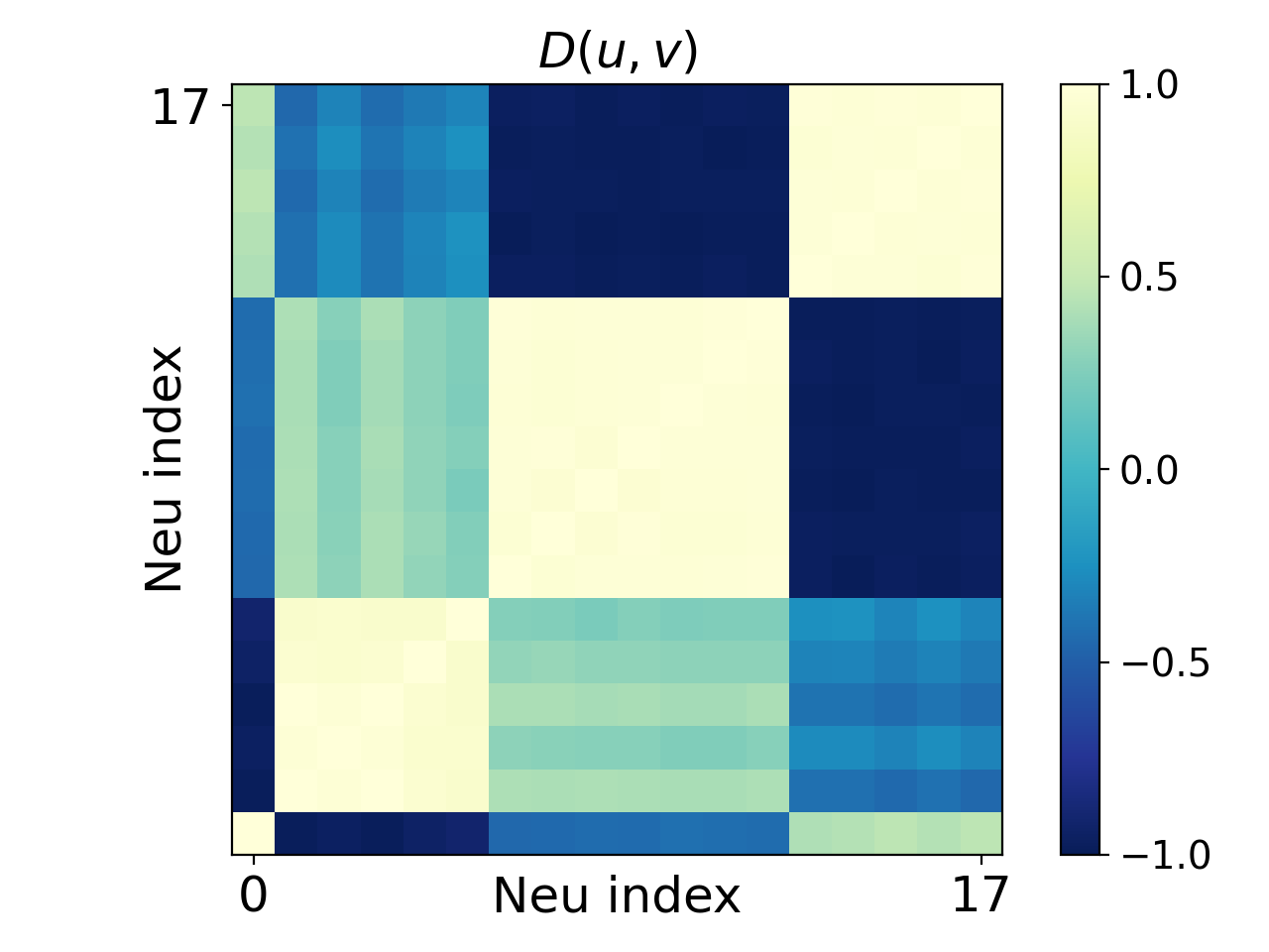
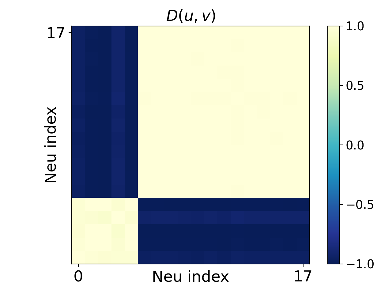
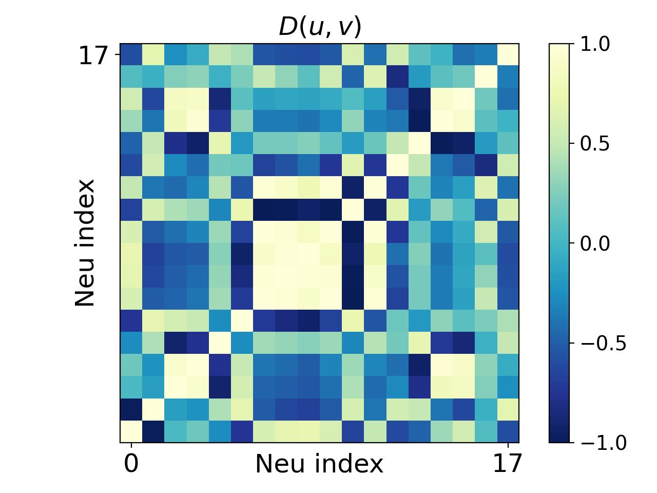
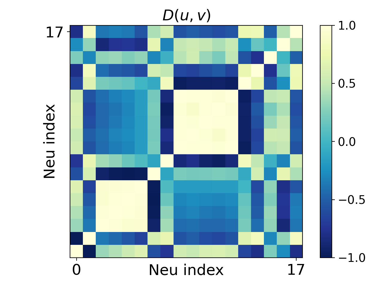
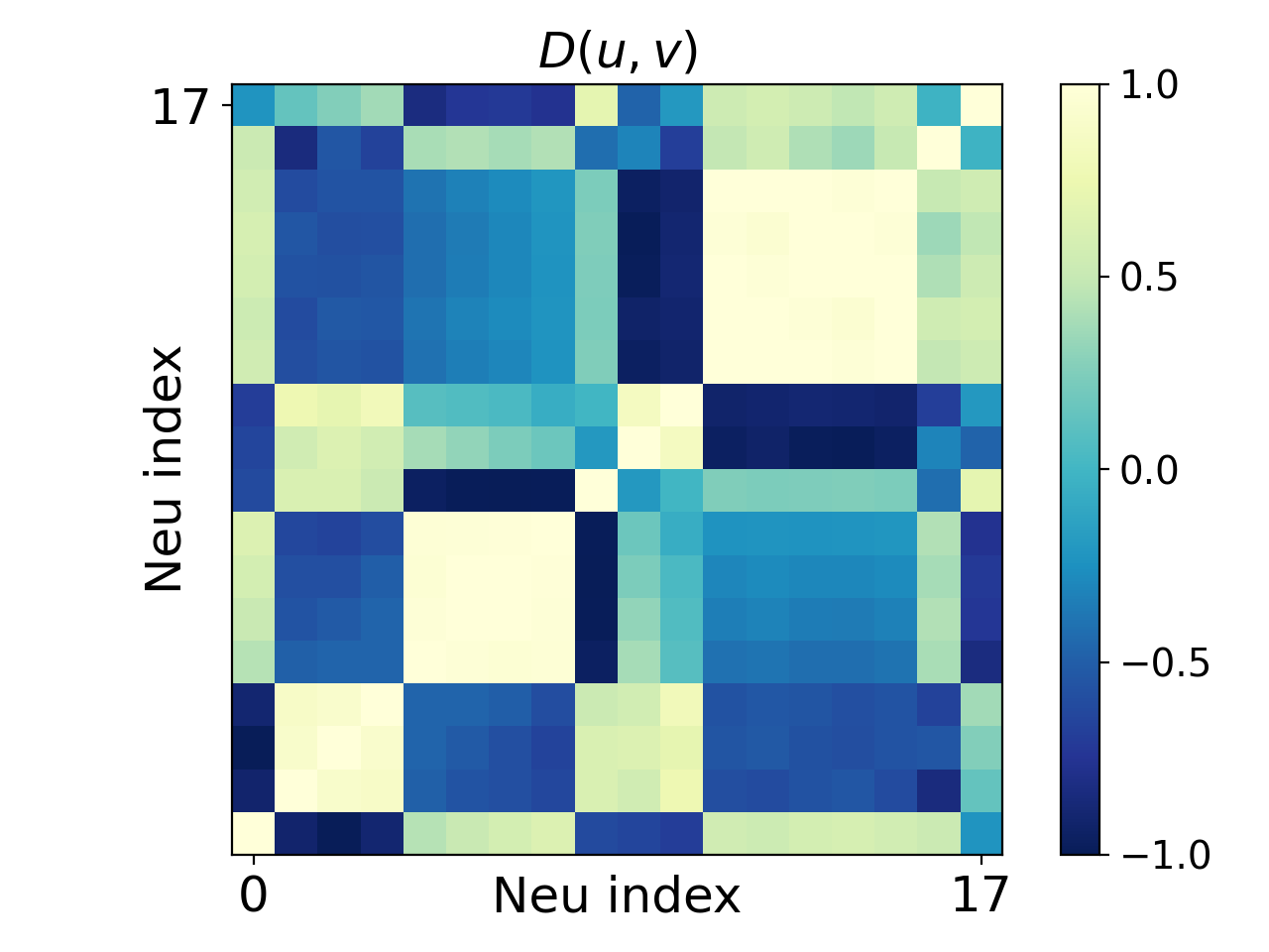
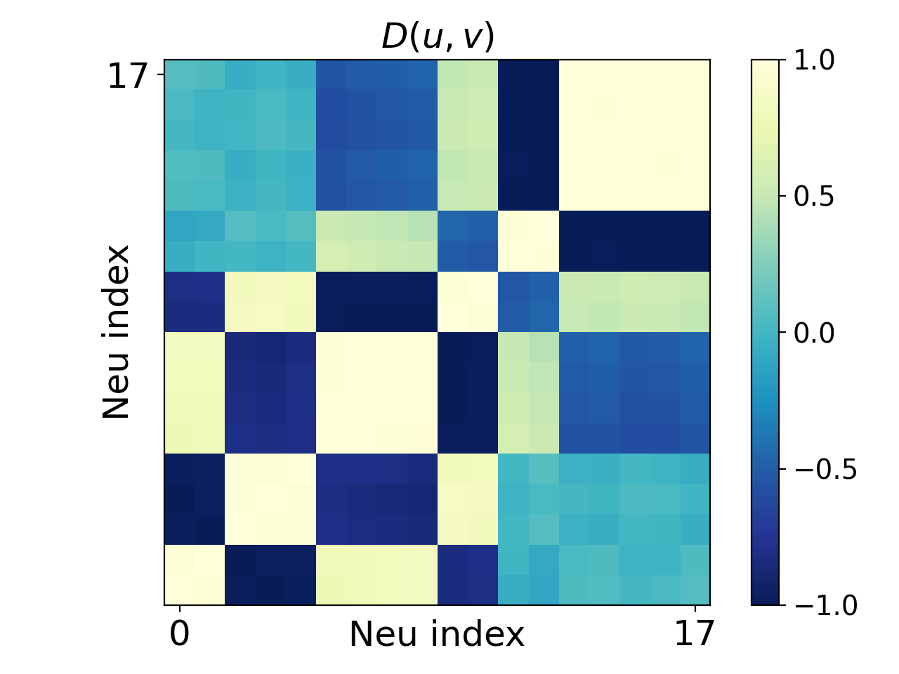
Figure 4: Condensation of six-layer NNs with residual connections. The activation functions for hidden layer 1 to hidden layer 5 are x2tanh(x)superscript𝑥2𝑥x^{2}\tanh(x), xtanh(x)𝑥𝑥x\tanh(x), sigmoid(x)sigmoid𝑥\mathrm{sigmoid}(x), tanh(x)𝑥\tanh(x) and softplus(x)softplus𝑥\mathrm{softplus}(x), respectively. The numbers of steps selected in the sub-pictures are epoch 1000, epoch 900, epoch 900, epoch 1400 and epoch 1400, respectively, while the NN is only trained once. The color indicates D(𝒖,𝒗)𝐷𝒖𝒗D(\bm{u},\bm{v}) of two hidden neurons’ input weights, whose indexes are indicated by the abscissa and the ordinate, respectively. The training data is 808080 points sampled from a 3-dimensional function k=134sin(12xk+1)superscriptsubscript𝑘13412subscript𝑥𝑘1\sum_{k=1}^{3}4\sin(12x_{k}+1), where each xksubscript𝑥𝑘x_{k} is uniformly sampled from [4,2]42[-4,2]. n=80𝑛80n=80, d=3𝑑3d=3, m=18𝑚18m=18, dout=1subscript𝑑out1d_{\mathrm{out}}=1, var=0.012varsuperscript0.012\mathrm{var}=0.01^{2}, lr=4×10⁵lr4superscript105\mathrm{lr}=4\times 10^{-5}.

For multi-layer NNs with different activation functions, we show that the condensation for all hidden layers is similar to the two-layer NNs. In deep networks, residual connection is often introduced to overcome the vanishing of gradient. To show the generality of condensation, we perform an experiment of six-layer NNs with residual connections. To show the difference of various activation functions, we set the activation functions for hidden layer 1 to hidden layer 5 as x2tanh(x)superscript𝑥2𝑥x^{2}\tanh(x), xtanh(x)𝑥𝑥x\tanh(x), sigmoid(x)sigmoid𝑥\mathrm{sigmoid}(x), tanh(x)𝑥\tanh(x) and softplus(x)softplus𝑥\mathrm{softplus}(x), respectively. The structure of the residual is 𝒉l+1(𝒙)=σ(𝑾l𝒉l(𝒙)+𝒃l)+𝒉l(𝒙)subscript𝒉𝑙1𝒙𝜎subscript𝑾𝑙subscript𝒉𝑙𝒙subscript𝒃𝑙subscript𝒉𝑙𝒙\bm{h}_{l+1}(\bm{x})=\sigma(\bm{W}_{l}\bm{h}_{l}(\bm{x})+\bm{b}_{l})+\bm{h}_{l}(\bm{x}), where 𝒉l(𝒙)subscript𝒉𝑙𝒙\bm{h}_{l}(\bm{x}) is the output of the l𝑙l-th layer. As shown in Fig. 4, input weights condense at three, two, one, one and one lines for hidden layer 1 to hidden layer 5, respectively. Note that residual connections are not necessary. We show an experiment of the same structure as in Fig. 4 but without residual connections in Appendix A.5.

Through these experiments, we conjecture that the maximal number of condensed orientations at initial training is twice the multiplicity of the activation function used. To understand the mechanism of the initial condensation, we turn to experiments of 1-d input and two-layer NNs, which can be clearly visualized in the next subsection.

4.4 1-d input and two-layer NN

For 1-d data, we visualize the evolution of the two-layer NN output and each weight, which confirms the connection between the condensation and the multiplicity of the activation function.
Refer to caption
(a) tanh(x)𝑥\tanh(x)
Refer to caption
(b) xtanh(x)𝑥𝑥x\tanh(x)
Refer to caption
(c) x2tanh(x)superscript𝑥2𝑥x^{2}\tanh(x)
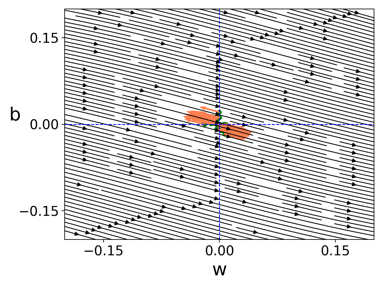
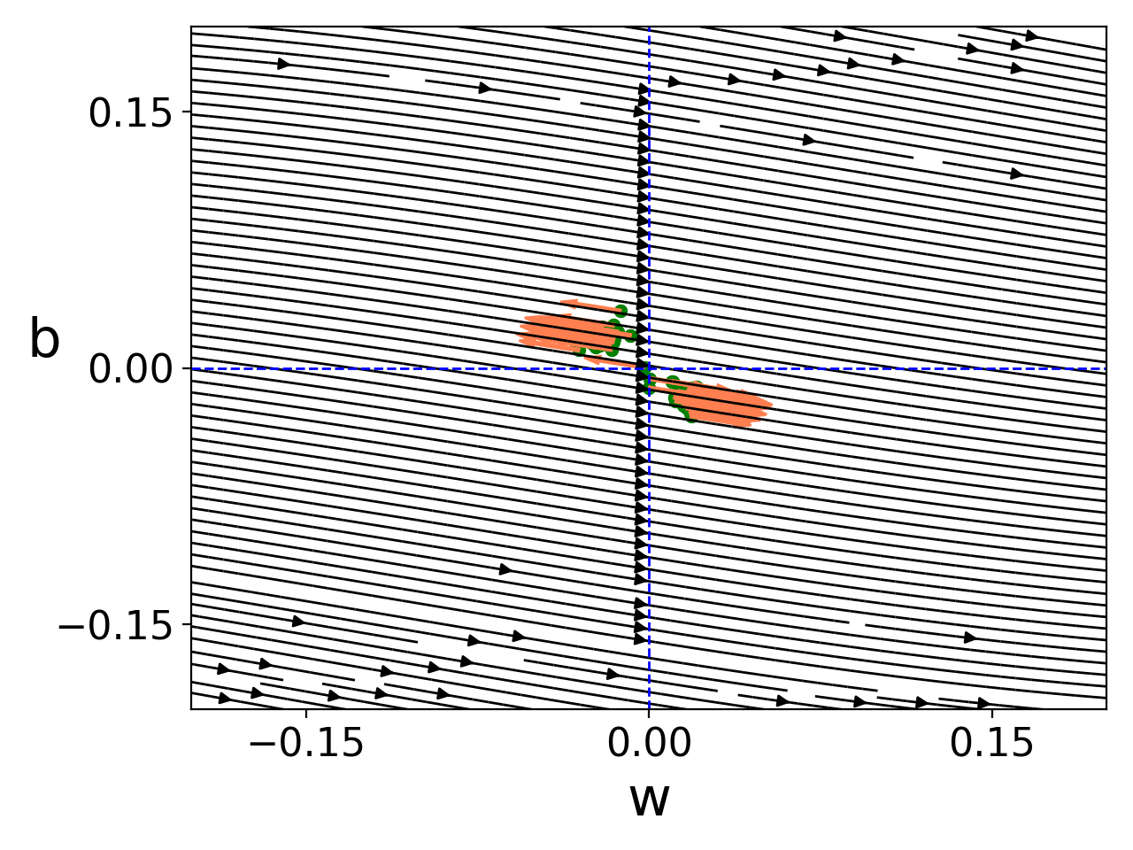
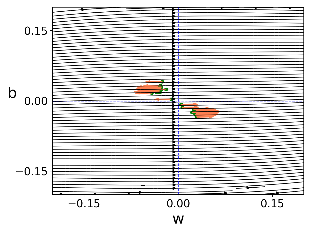
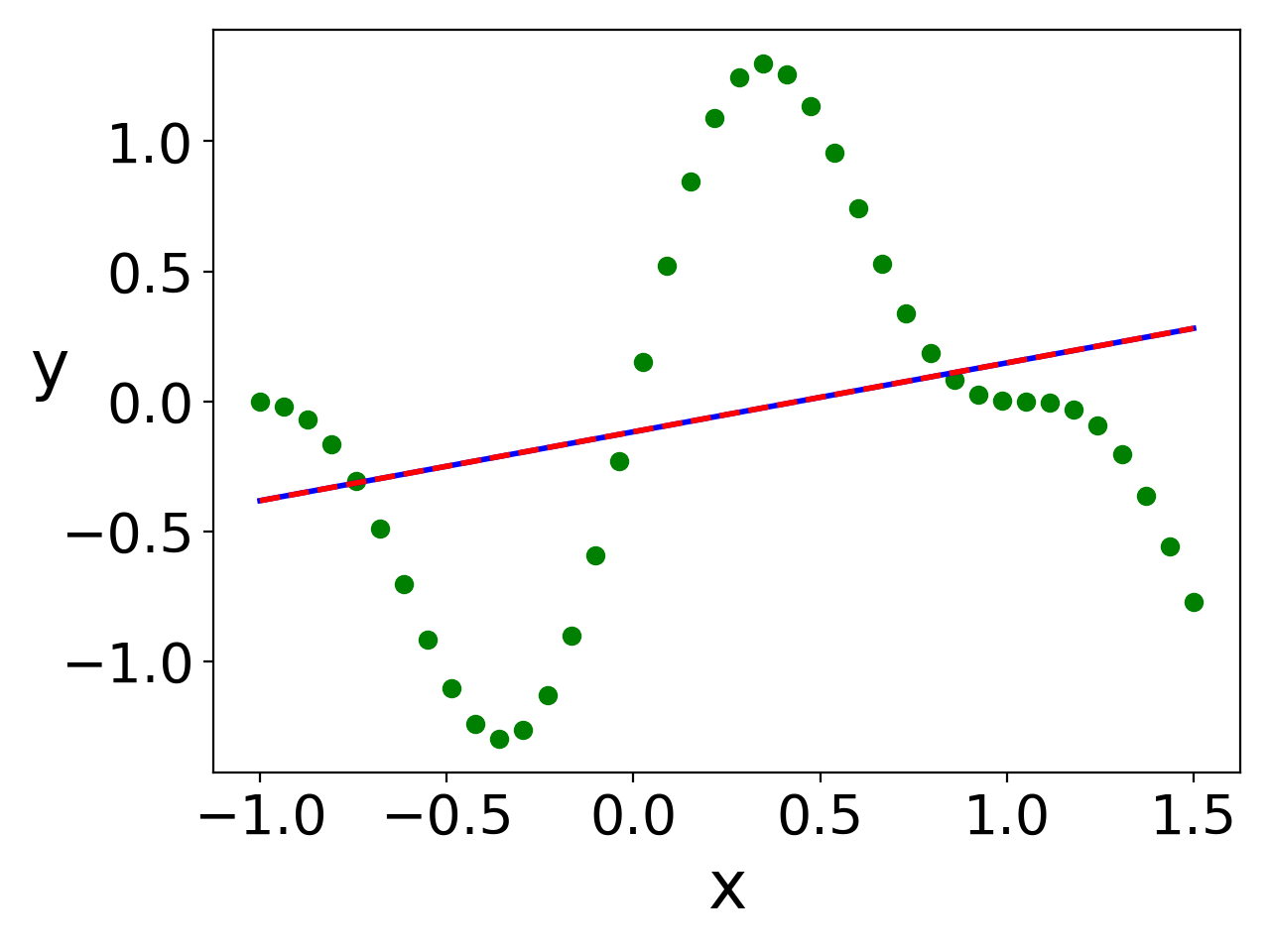
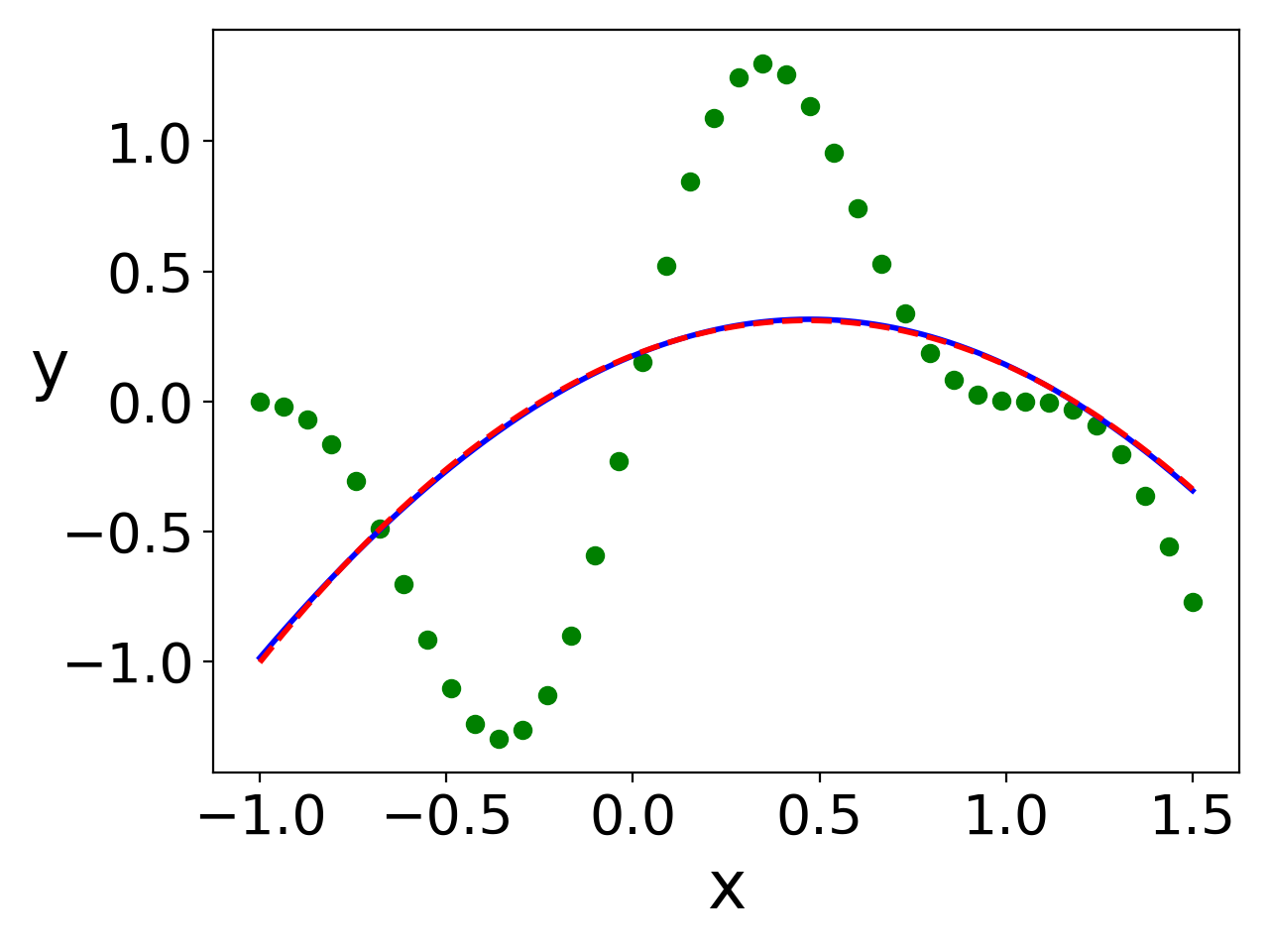
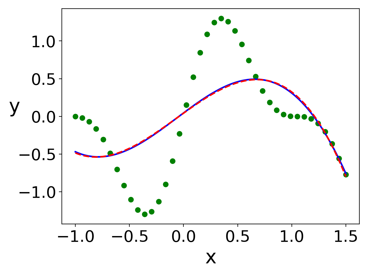
Figure 5: The outputs of two-layer NNs at epoch 100010001000 with activation function tanh(x)𝑥\tanh(x), xtanh(x)𝑥𝑥x\tanh(x), and x2tanh(x)superscript𝑥2𝑥x^{2}\tanh(x) are displayed, respectively. The training data is 404040 points uniformly sampled from sin(3x)+sin(6x)/23𝑥6𝑥2\sin(3x)+\sin(6x)/2 with x[1,1.5]𝑥11.5x\in[-1,1.5], illustrated by green dots. The blue solid lines are the NN outputs at test points, while the red dashed auxiliary lines are the first, second, third and first order polynomial fittings of the test points for (a, b, c), respectively. Parameters are n=40𝑛40n=40, d=1𝑑1d=1, m=100𝑚100m=100, dout=1subscript𝑑out1d_{\mathrm{out}}=1, var=0.0052varsuperscript0.0052\mathrm{var}=0.005^{2}, lr=5×10⁴lr5superscript104\mathrm{lr}=5\times 10^{-4}.

We display the outputs at initial training in Fig. 5. Due to the small magnitude of parameters, an activation function with multiplicity p𝑝p can be well approximated by a p𝑝p-th order polynominal, thus, the NN output can also be approximated by a p𝑝p-th order polynominal. As shown in Fig. 5, the NN outputs with activation function tanh(x)𝑥\tanh(x), xtanh(x)𝑥𝑥x\tanh(x) and x2tanh(x)superscript𝑥2𝑥x^{2}\tanh(x) overlap well with the auxiliary of a linear, a quadratic and a cubic polynominal curve, respectively in the beginning. This experiment, although simple, but convincingly shows that NN does not always learn a linear function at the initial training stage and the complexity of such learning depends on the activation function.

Refer to caption
(a) tanh(x)𝑥\tanh(x)
Refer to caption
(b) xtanh(x)𝑥𝑥x\tanh(x)
Refer to caption
(c) x2tanh(x)superscript𝑥2𝑥x^{2}\tanh(x)
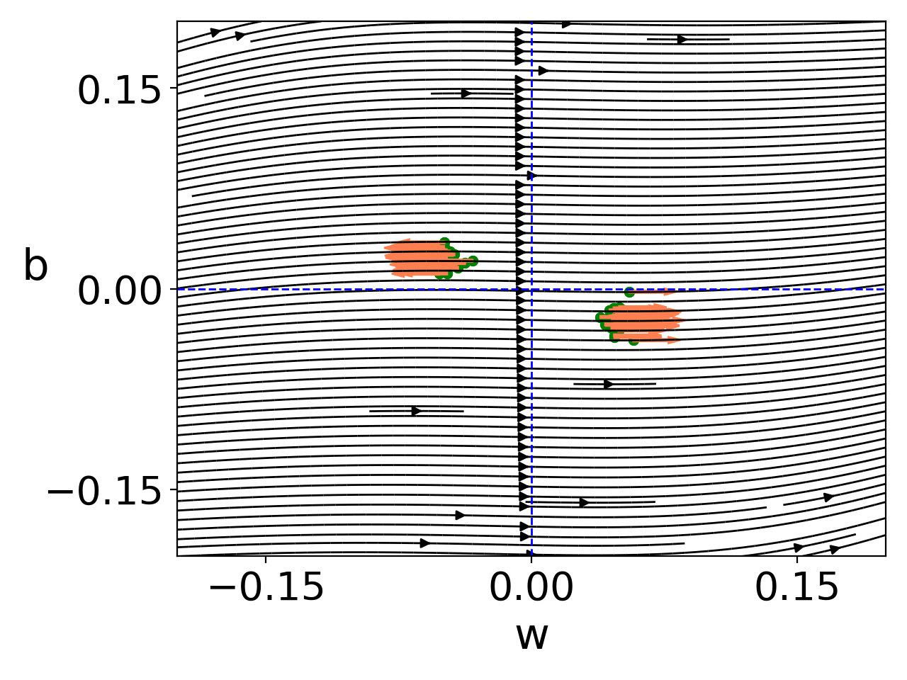
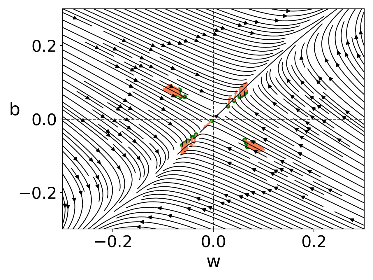
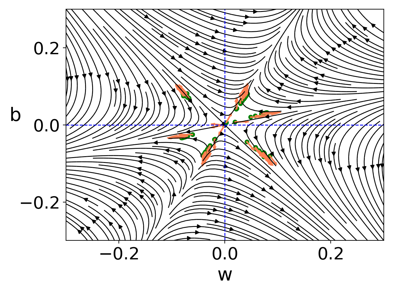
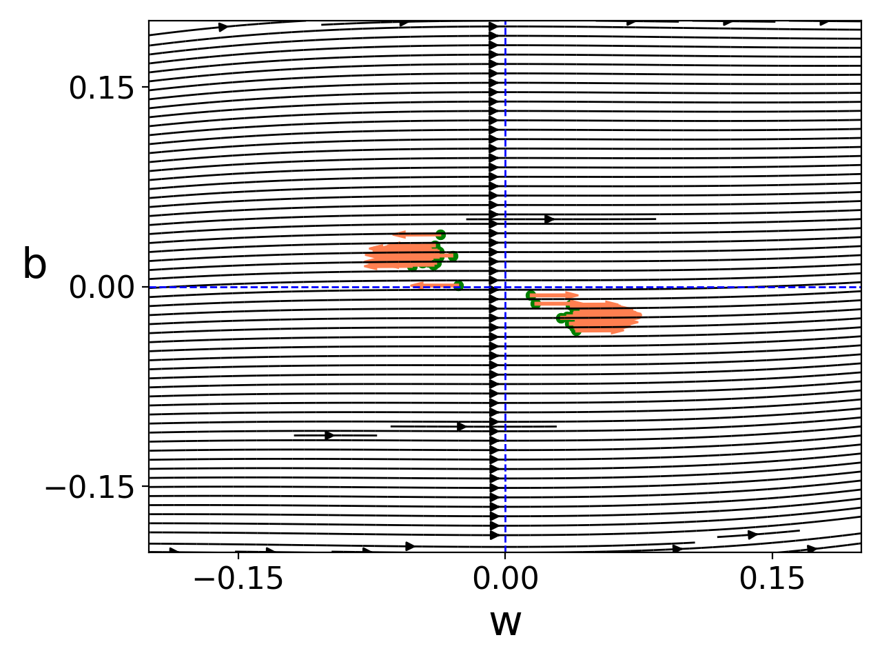
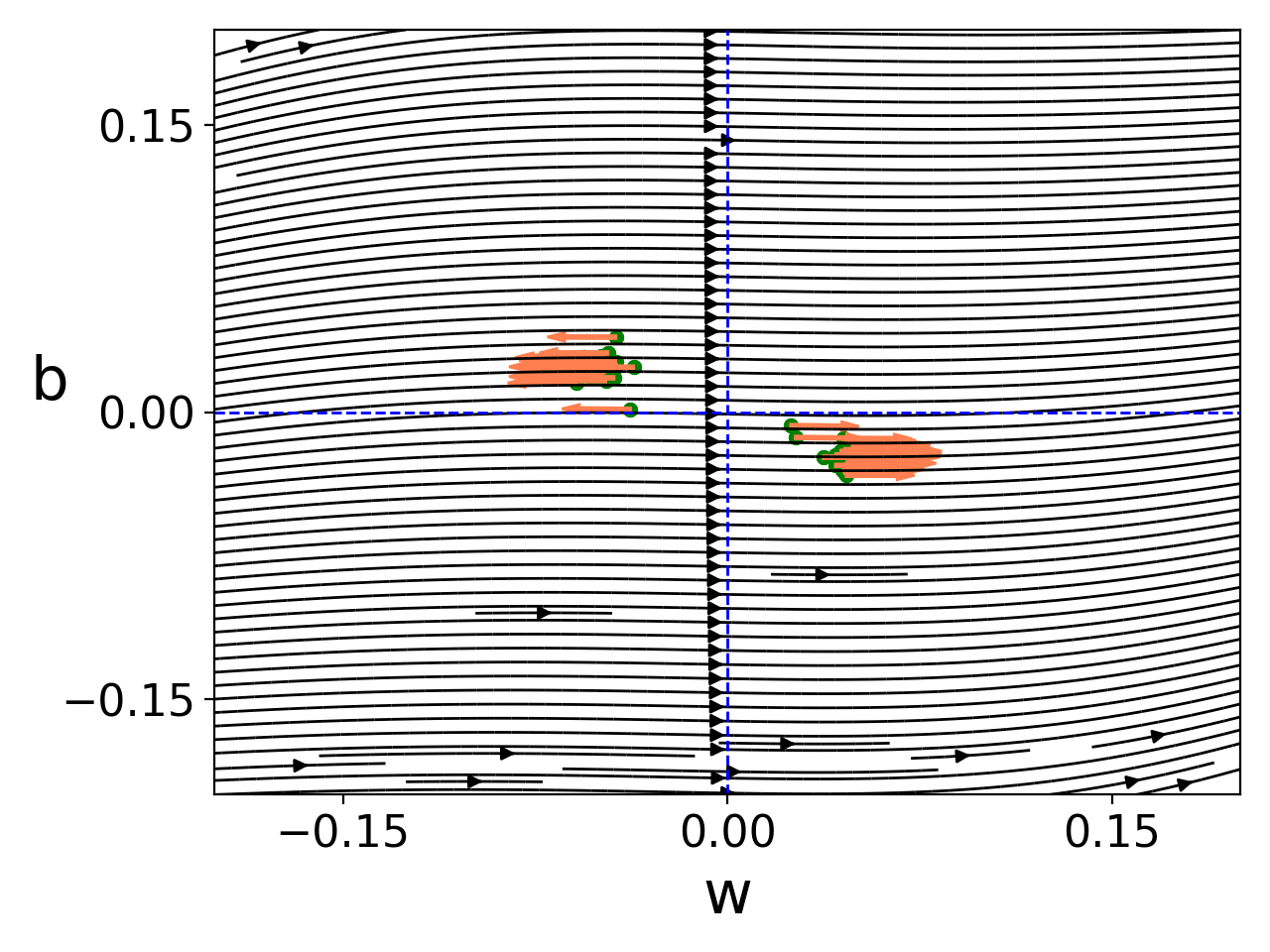
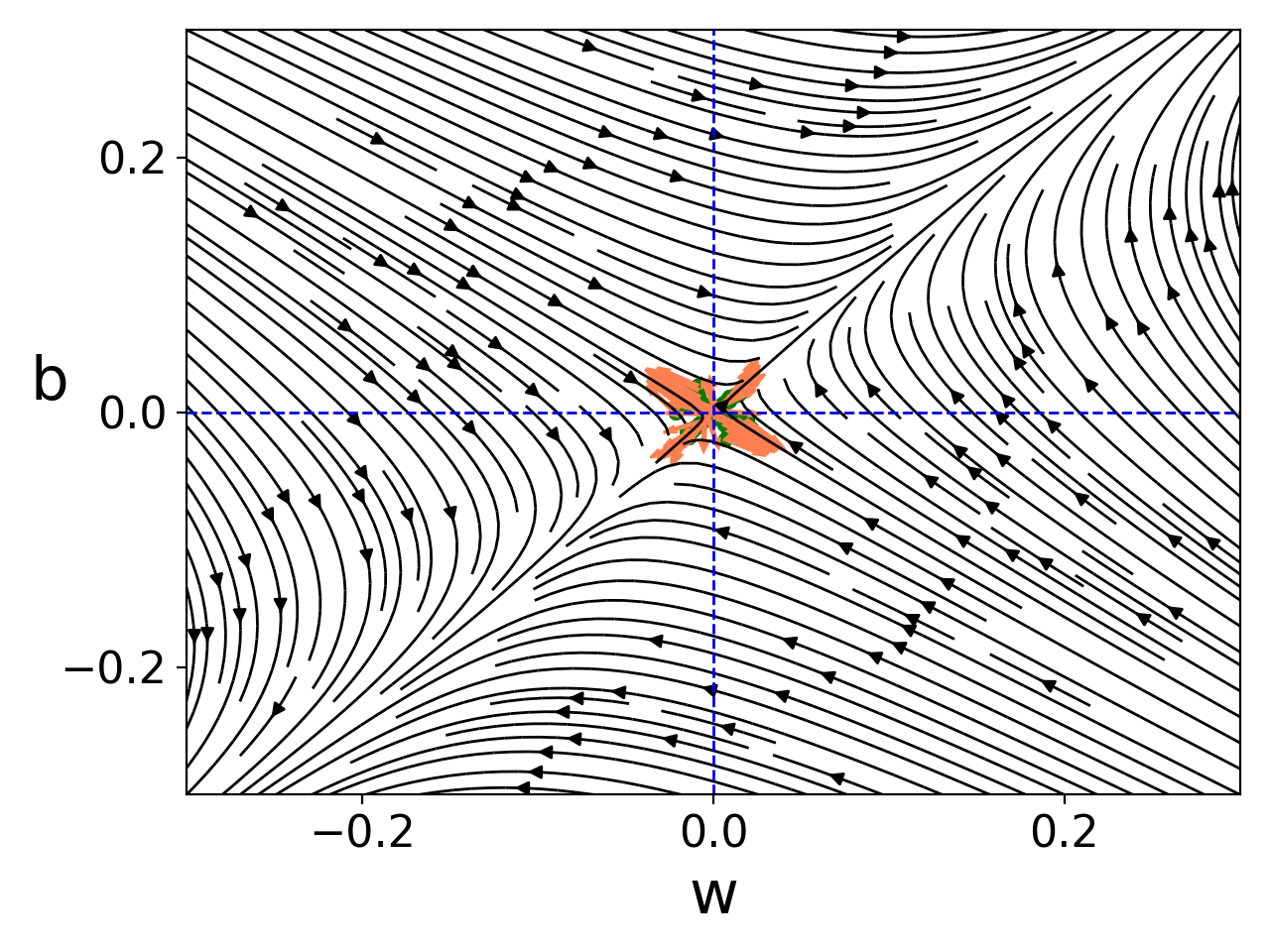
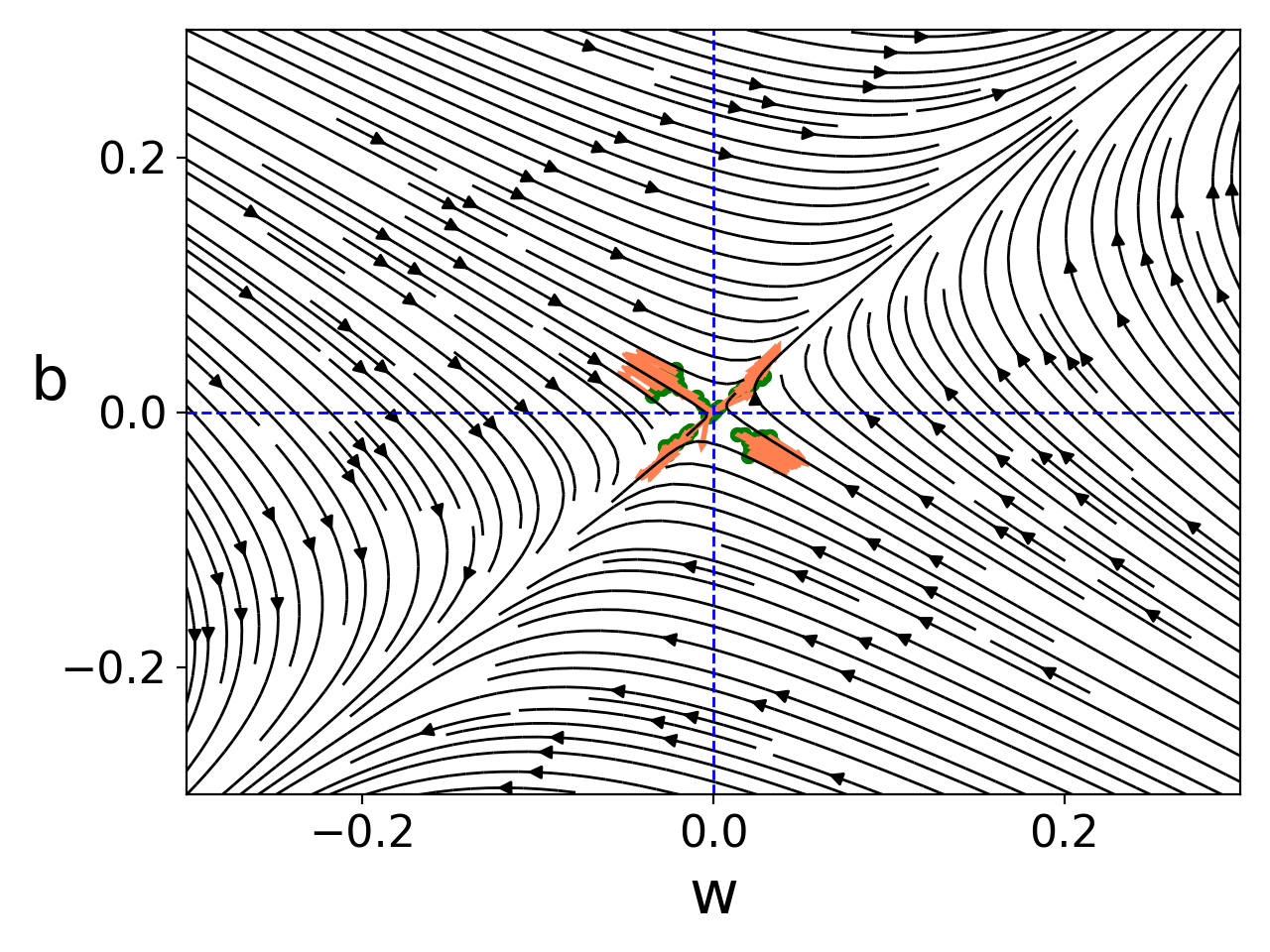
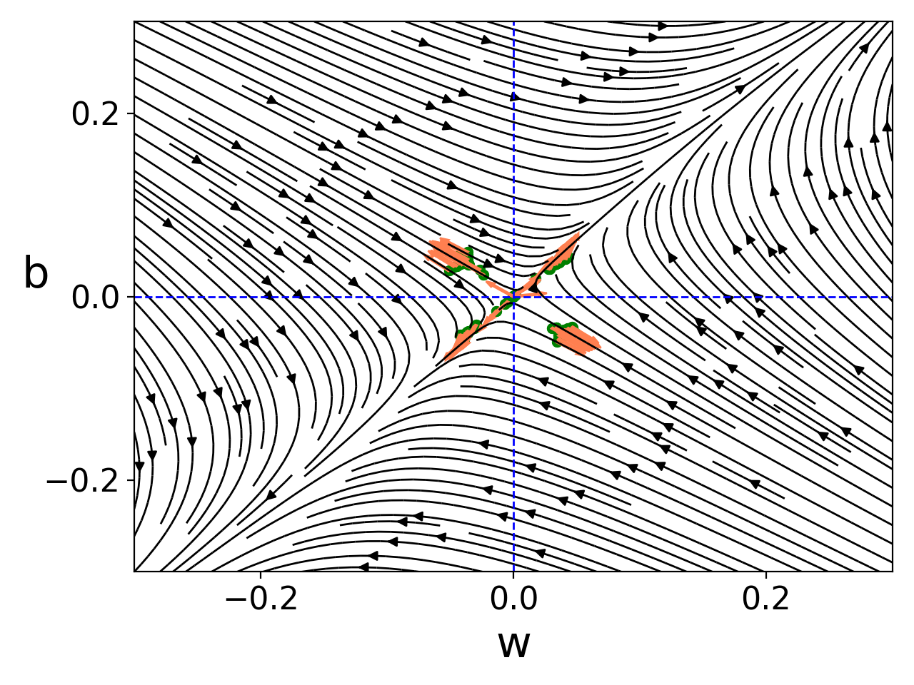
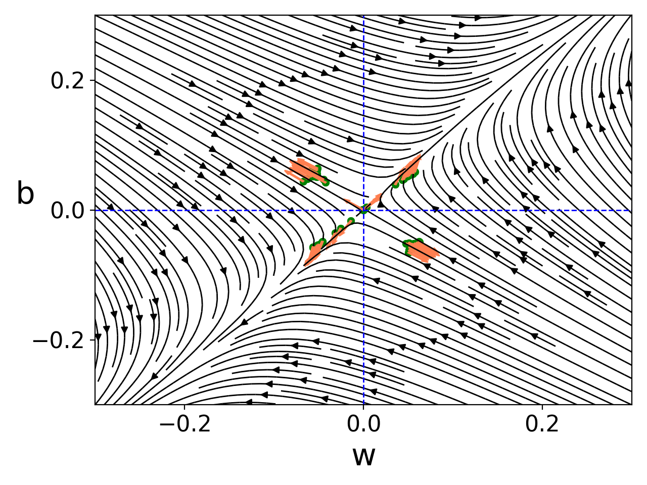
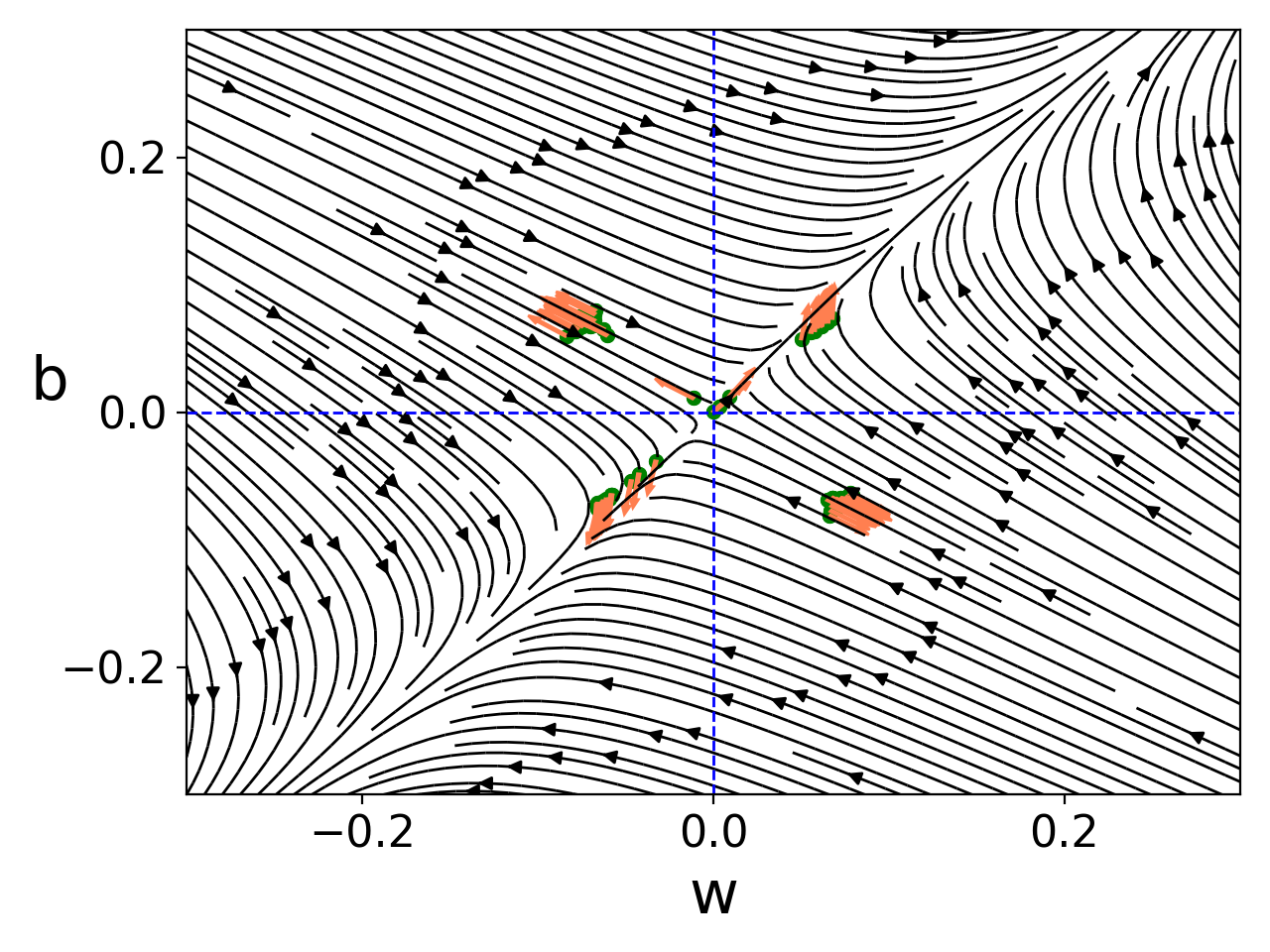
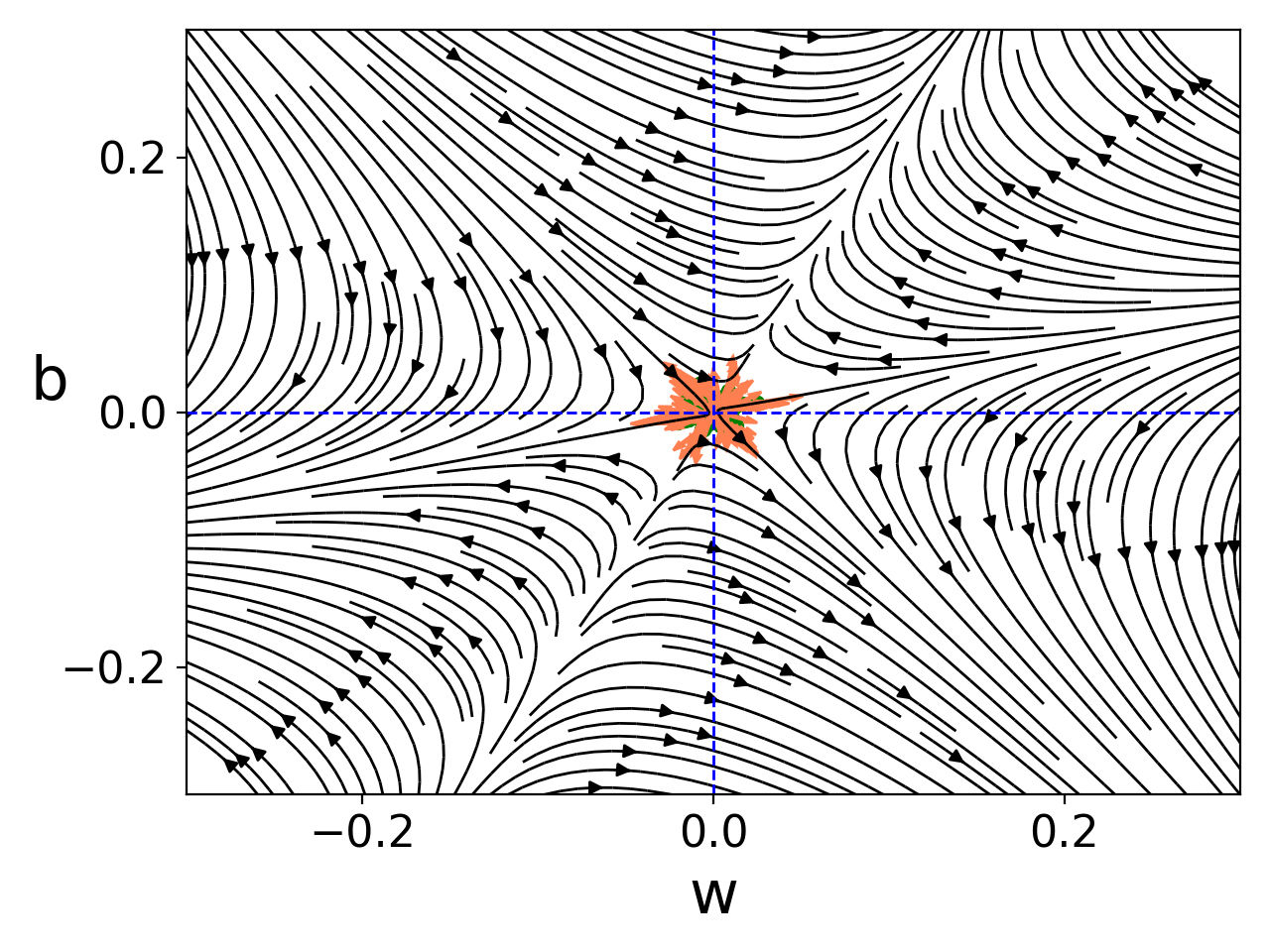
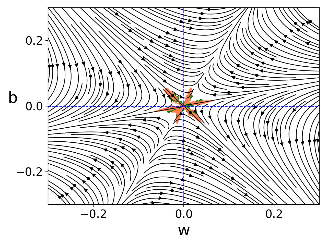
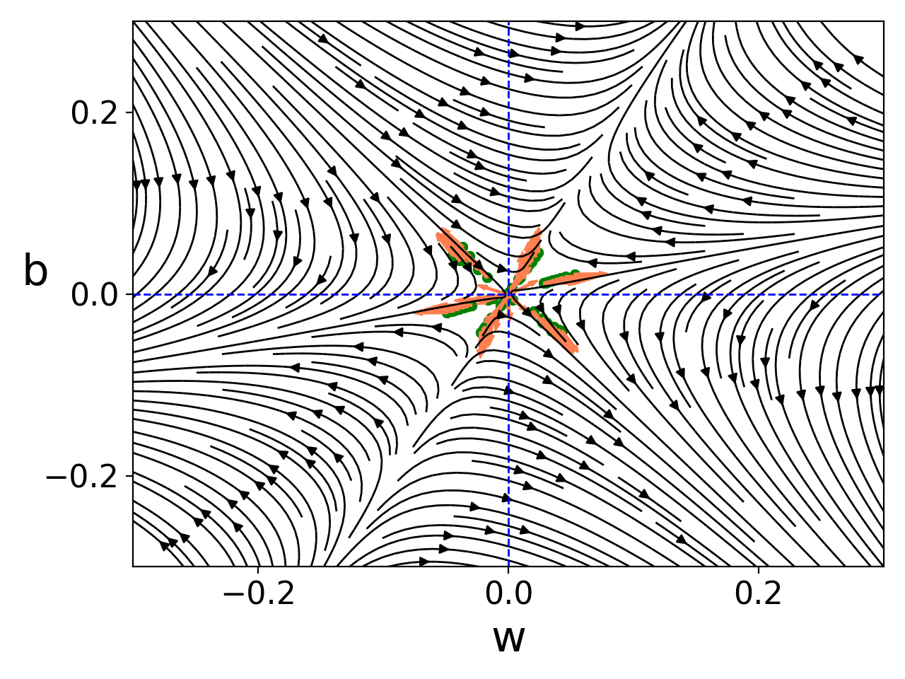
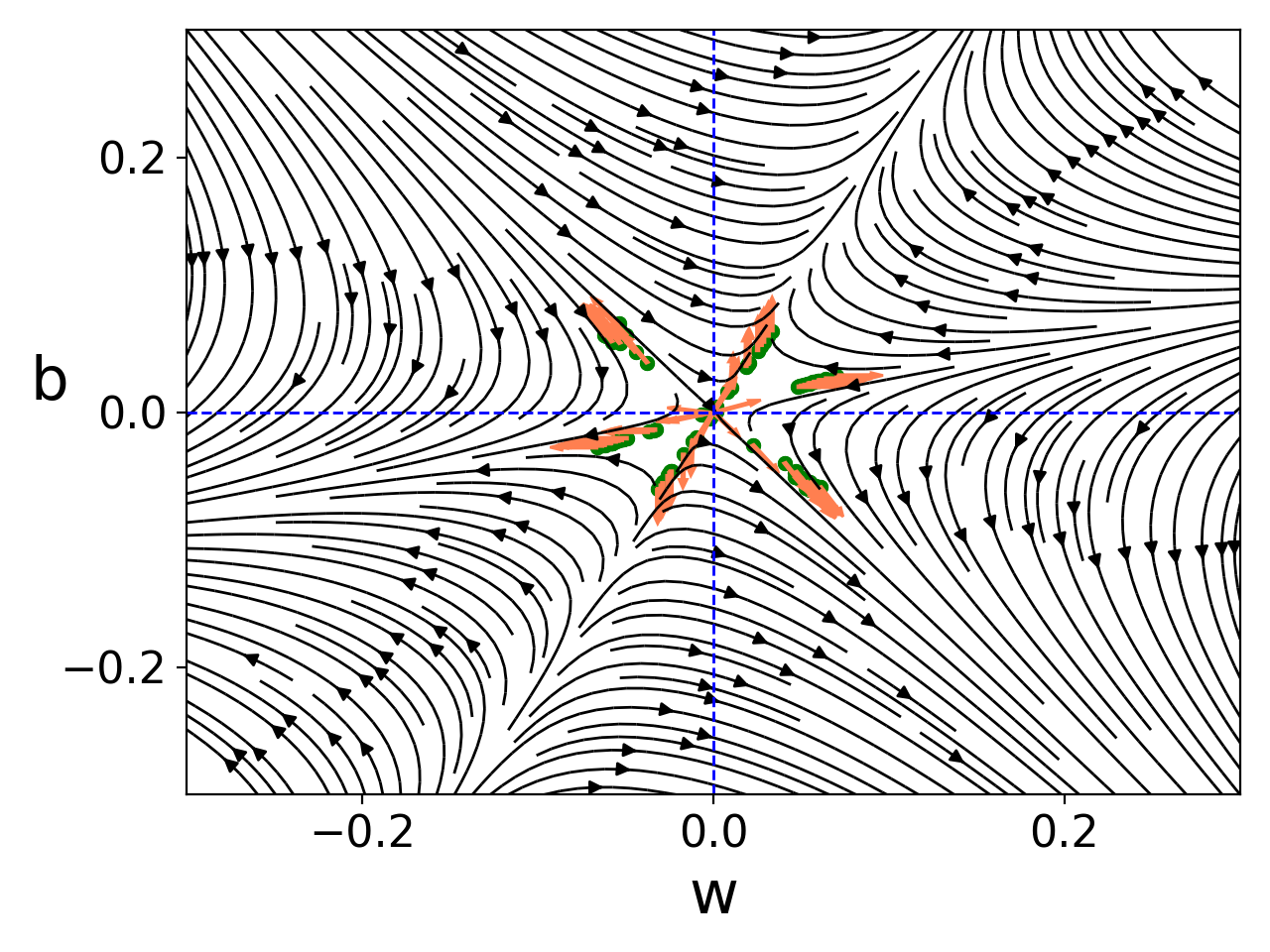
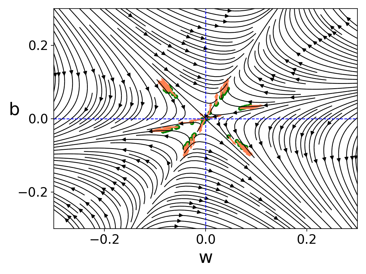
Figure 6: The direction field for input weight 𝒘:=(w,b)assign𝒘𝑤𝑏\bm{w}:=(w,b) of the dynamics in (4.4) at epoch 200. All settings are the same as Fig. 5. Around the original point, the field has one, two, three stables lines, on which an input weight would keep its direction, for tanh(x)𝑥\tanh(x), xtanh(x)𝑥𝑥x\tanh(x), and x2tanh(x)superscript𝑥2𝑥x^{2}\tanh(x), respectively. We also display the value of each weight by the green dots and the corresponding directions by the orange arrows.

We visualize the direction field for input weight 𝒘j:=(wj,bj)assignsubscript𝒘𝑗subscript𝑤𝑗subscript𝑏𝑗\bm{w}_{j}:=(w_{j},b_{j}), following the gradient flow,

𝒘j˙=ajni=1neiσ(𝒘j𝒙i)𝒙i,˙subscript𝒘𝑗subscript𝑎𝑗𝑛superscriptsubscript𝑖1𝑛subscript𝑒𝑖superscript𝜎subscript𝒘𝑗subscript𝒙𝑖subscript𝒙𝑖\dot{\bm{w}_{j}}=-\frac{a_{j}}{n}\sum_{i=1}^{n}e_{i}\sigma^{\prime}(\bm{w}_{j}\cdot\bm{x}_{i})\bm{x}_{i},

where ei:=f𝜽(𝒙i)f(𝒙i)assignsubscript𝑒𝑖subscript𝑓𝜽subscript𝒙𝑖superscript𝑓subscript𝒙𝑖e_{i}:=f_{\bm{\theta}}(\bm{x}_{i})-f^{*}(\bm{x}_{i}). Since we only care about the direction of 𝒘jsubscript𝒘𝑗\bm{w}_{j} and ajsubscript𝑎𝑗a_{j} is a scalar at each epoch, we can visualize 𝒘j˙˙subscript𝒘𝑗\dot{\bm{w}_{j}} by 𝒘j˙/aj˙subscript𝒘𝑗subscript𝑎𝑗\dot{\bm{w}_{j}}/a_{j}. For simplicity, we do not distinguish 𝒘j˙/aj˙subscript𝒘𝑗subscript𝑎𝑗\dot{\bm{w}_{j}}/a_{j} and 𝒘j˙˙subscript𝒘𝑗\dot{\bm{w}_{j}} if there is no ambiguity. When we compute 𝒘j˙˙subscript𝒘𝑗\dot{\bm{w}_{j}} for different j𝑗j’s, ei𝒙isubscript𝑒𝑖subscript𝒙𝑖e_{i}\bm{x}_{i} for (i=1,,n𝑖1𝑛i=1,\cdots,n) is independent with j𝑗j. Then, at each epoch, for a set of {ei,𝒙i}i=1nsuperscriptsubscriptsubscript𝑒𝑖subscript𝒙𝑖𝑖1𝑛\{e_{i},\bm{x}_{i}\}_{i=1}^{n}, we can consider the following direction field

𝝎˙=1ni=1nei𝒙iσ(𝝎𝒙i).˙𝝎1𝑛superscriptsubscript𝑖1𝑛subscript𝑒𝑖subscript𝒙𝑖superscript𝜎𝝎subscript𝒙𝑖\dot{\bm{\omega}}=-\frac{1}{n}\sum_{i=1}^{n}e_{i}\bm{x}_{i}\sigma^{\prime}(\bm{\omega}\cdot\bm{x}_{i}).

When 𝝎𝝎\bm{\omega} is set as 𝒘jsubscript𝒘𝑗\bm{w}_{j}, we can obtain 𝒘j˙˙subscript𝒘𝑗\dot{\bm{w}_{j}}. As shown in Fig. 6, around the original point, the field has one, two, three stables lines, on which a neuron would keep its direction, for tanh(x)𝑥\tanh(x), xtanh(x)𝑥𝑥x\tanh(x), and x2tanh(x)superscript𝑥2𝑥x^{2}\tanh(x), respectively. We also display the input weight of each neuron on the field by the green dots and their corresponding velocity directions by the orange arrows. Similarly to the high-dimensional cases, NNs with multiplicity p𝑝p activation functions condense at p𝑝p different lines for p=1,2,3𝑝123p=1,2,3. Therefore, It is reasonable to conjecture that the maximal number of condensed orientations is twice the multiplicity of the activation function used.

Taken together, we have empirically shown that the multiplicity of the activation function is a key factor that determines the complexity of the initial output and condensation. To facilitate the understanding of the evolution of condensation in the initial stage, we show several steps during the initial stage of each example in Appendix A.6.

5 Analysis of the initial condensation of input weights

In this section, we would present a preliminary analysis to understand how the multiplicity of the activation function affects the initial condensation. At each training step, we consider the velocity field of weights in each hidden layer of a neural networks.

Considering a network with L𝐿L hidden layers, we use row vector 𝑾j[k]subscriptsuperscript𝑾delimited-[]𝑘𝑗{\bm{W}^{[k]}_{j}} to represent the weight from the (k1)𝑘1(k-1)-th layer to the j𝑗j-th neuron in the k𝑘k-th layer. Since condensation is always accompany with small initialization, together with the initial stage defined in Sec. 3, we make the following assumptions,

Assumption 1.

Small initialization infers that 𝑾j[k]𝒙[k1]o(1)similar-tosubscriptsuperscript𝑾delimited-[]𝑘𝑗superscript𝒙delimited-[]𝑘1𝑜1\bm{W}^{[k]}_{j}\bm{x}^{[k-1]}\sim o(1) applies for all k𝑘k’s and j𝑗j’s.

Assumption 2.

During the initial stage of condensation, Taylor expansion of each corresponding activated neurons holds, i.e.,

σ(𝑾j[k]𝒙[k1])=σ(0)++σ(γ)(0)(γ1)!(𝑾j[k]𝒙[k1])γ1+O((𝑾j[k]𝒙[k1])γ)superscript𝜎subscriptsuperscript𝑾delimited-[]𝑘𝑗superscript𝒙delimited-[]𝑘1superscript𝜎0superscript𝜎𝛾0𝛾1superscriptsubscriptsuperscript𝑾delimited-[]𝑘𝑗superscript𝒙delimited-[]𝑘1𝛾1𝑂superscriptsubscriptsuperscript𝑾delimited-[]𝑘𝑗superscript𝒙delimited-[]𝑘1𝛾\sigma^{\prime}(\bm{W}^{[k]}_{j}\bm{x}^{[k-1]})=\sigma^{\prime}(0)+\dots+\frac{\sigma^{(\gamma)}(0)}{(\gamma-1)!}(\bm{W}^{[k]}_{j}\bm{x}^{[k-1]})^{\gamma-1}+O((\bm{W}^{[k]}_{j}\bm{x}^{[k-1]})^{\gamma}) (6)

Suppose the activation function has multiplicity p𝑝p, i.e., σ(s)(0)=0superscript𝜎𝑠00\sigma^{(s)}(0)=0 for s=1,2,,p1𝑠12𝑝1s=1,2,\cdots,p-1, and σ(p)(0)0superscript𝜎𝑝00\sigma^{(p)}(0)\neq 0. Then, together with Assumption 2, we have

σ(𝑾j[k]𝒙[k1])σ(p)(0)(p1)!(𝑾j[k]𝒙[k1])p1.superscript𝜎subscriptsuperscript𝑾delimited-[]𝑘𝑗superscript𝒙delimited-[]𝑘1superscript𝜎𝑝0𝑝1superscriptsubscriptsuperscript𝑾delimited-[]𝑘𝑗superscript𝒙delimited-[]𝑘1𝑝1\sigma^{\prime}(\bm{W}^{[k]}_{j}\bm{x}^{[k-1]})\approx\frac{\sigma^{(p)}(0)}{(p-1)!}(\bm{W}^{[k]}_{j}\bm{x}^{[k-1]})^{p-1}. (7)

For each k𝑘k and j𝑗j, 𝑾j[k]subscriptsuperscript𝑾delimited-[]𝑘𝑗{\bm{W}^{[k]}_{j}} satisfies the following dynamics, (see Appendix A.2)

r˙=𝒖𝒘˙,𝒖˙=𝒘˙(𝒘˙𝒖)𝒖r.formulae-sequence˙𝑟𝒖˙𝒘˙𝒖˙𝒘˙𝒘𝒖𝒖𝑟\dot{r}=\bm{u}\cdot\dot{\bm{w}},\quad\dot{\bm{u}}=\frac{\dot{\bm{w}}-(\dot{\bm{w}}\cdot\bm{u})\bm{u}}{r}. (8)

where 𝒘𝒘\bm{w} can represent 𝑾j[k]superscriptsubscriptsuperscript𝑾delimited-[]𝑘𝑗{\bm{W}^{[k]}_{j}}^{\intercal} for all k𝑘k’s and j𝑗j’s, r=𝒘2𝑟subscriptnorm𝒘2r=\|\bm{w}\|_{2} is the amplitude, and 𝒖=𝒘/r𝒖𝒘𝑟\bm{u}=\bm{w}/r.

For convenience, we define an operator 𝒫𝒫\mathcal{P} satisfying 𝒫𝒘:=𝒘˙𝒖(𝒘˙𝒖).assign𝒫𝒘˙𝒘𝒖˙𝒘𝒖\mathcal{P}\bm{w}:=\dot{\bm{w}}-\bm{u}(\dot{\bm{w}}\cdot\bm{u}). To specify the condensation for theoretical analysis, we make the following definition,

Condensation: the weight evolves towards a direction which will not change in the direction field and is defined as follows,

𝒖˙=0𝒫𝒘:=𝒘˙𝒖(𝒘˙𝒖)=0.˙𝒖0assign𝒫𝒘˙𝒘𝒖˙𝒘𝒖0\dot{\bm{u}}=0\ \Leftrightarrow\ \mathcal{P}\bm{w}:=\dot{\bm{w}}-\bm{u}(\dot{\bm{w}}\cdot\bm{u})=0. (9)

Since 𝒘˙𝒖˙𝒘𝒖\dot{\bm{w}}\cdot\bm{u} is a scalar, 𝒘˙˙𝒘\dot{\bm{w}} is parallel with 𝒖𝒖\bm{u}. 𝒖𝒖\bm{u} is a unit vector, therefore, we have 𝒖=±𝒘˙/𝒘˙2𝒖plus-or-minus˙𝒘subscriptnorm˙𝒘2\bm{u}=\pm\dot{\bm{w}}/\|\dot{\bm{w}}\|_{2}.

Remark 1 (An intuitive explanation for condensation).

In this work, we consider NNs with sufficiently small parameters. Suppose r=𝒘2O(ϵ)𝑟subscriptnorm𝒘2similar-to𝑂italic-ϵr=\|\bm{w}\|_{2}\sim O(\epsilon), where ϵitalic-ϵ\epsilon is a small quantity, then dynamics (8) will show that O(r˙)O(𝒘˙)similar-to𝑂˙𝑟𝑂˙𝒘O(\dot{r})\sim O(\dot{\bm{w}}) and O(𝒖˙)O(r˙)/O(ϵ)similar-to𝑂˙𝒖𝑂˙𝑟𝑂italic-ϵO(\dot{\bm{u}})\sim O(\dot{r})/O(\epsilon). Here O(r˙)O(𝒘˙)similar-to𝑂˙𝑟𝑂˙𝒘O(\dot{r})\sim O(\dot{\bm{w}}) refers that the evolution of r˙˙𝑟\dot{r} is at the same order as every component of 𝒘˙˙𝒘\dot{\bm{w}}, and it is the same for O(𝒖˙)O(r˙)/O(ϵ)similar-to𝑂˙𝒖𝑂˙𝑟𝑂italic-ϵO(\dot{\bm{u}})\sim O(\dot{r})/O(\epsilon). Therefore, the orientation 𝒖𝒖\bm{u} would vary much more quickly than the amplitude r𝑟r. By the dynamics for 𝒘𝒘\bm{w} (Eq. 10) and the Taylor approximation with multiplicity p𝑝p (Eq. 7), it is easy to find that the solutions for Eq. 9 are finite. Then, taken together, the orientation 𝒖𝒖\bm{u} would converge rapidly into certain directions, leading to condensation.

In the following, we study the case of (i) p=1𝑝1p=1 and (ii) mk1=1subscript𝑚𝑘11m_{k-1}=1 (the dimension of input of the k𝑘k-th layer equals one), and reach the following informal proposition,

Proposition 1. Suppose that Assumption 1 and 2 holds. Consider the leading-order Taylor expansion of Eq. 9, as initialization towards zero. If either p=1𝑝1p=1 or mk1=1subscript𝑚𝑘11m_{k-1}=1 holds, then the maximal number of roots for Eq. 9 is twice of the multiplicity of the activation function.
Proof.

Case 1: p=1𝑝1p=1

By gradient flow, we can obtain the dynamics for 𝑾j[k]subscriptsuperscript𝑾delimited-[]𝑘𝑗{\bm{W}}^{[k]}_{j} (see Appendix A.2),

𝒘˙=𝑾˙j[k]=1ni=1n(f(𝜽,𝒙i)yi)[diag{σ(𝑾[k]𝒙i[k1])}(𝑬[k+1:L]𝒂)]j𝒙i[k1],superscript˙𝒘subscriptsuperscript˙𝑾delimited-[]𝑘𝑗1𝑛superscriptsubscript𝑖1𝑛𝑓𝜽subscript𝒙𝑖subscript𝑦𝑖subscriptdelimited-[]diagsuperscript𝜎superscript𝑾delimited-[]𝑘superscriptsubscript𝒙𝑖delimited-[]𝑘1superscript𝑬delimited-[]:𝑘1𝐿𝒂𝑗superscriptsuperscriptsubscript𝒙𝑖delimited-[]𝑘1\dot{\bm{w}}^{\intercal}={\dot{\bm{W}}^{[k]}_{j}}=-\frac{1}{n}\sum_{i=1}^{n}\left(f(\bm{\theta},\bm{x}_{i})-y_{i}\right)[\operatorname{diag}\{\sigma^{\prime}(\bm{W}^{[k]}\bm{x}_{i}^{[k-1]})\}(\bm{E}^{[k+1:L]}\bm{a})]_{j}{\bm{x}_{i}^{[k-1]}}^{\intercal}, (10)

where we use 𝑬l=𝑾[l]diag{σ(𝑾[l]𝒙[l1])},forl{2,3,,L}formulae-sequencesuperscript𝑬𝑙superscriptsuperscript𝑾delimited-[]𝑙diagsuperscript𝜎superscript𝑾delimited-[]𝑙superscript𝒙delimited-[]𝑙1for𝑙23𝐿\bm{E}^{l}={\bm{W}^{[l]}}^{\intercal}\operatorname{diag}\{\sigma^{\prime}(\bm{W}^{[l]}\cdot\bm{x}^{[l-1]})\},\ \text{for}\ l\in\{2,3,...,L\}, 𝑬[q:p]=𝑬q𝑬q+1𝑬psuperscript𝑬delimited-[]:𝑞𝑝superscript𝑬𝑞superscript𝑬𝑞1superscript𝑬𝑝\bm{E}^{[q:p]}=\bm{E}^{q}\bm{E}^{q+1}...\bm{E}^{p}, and 𝒙i[k]superscriptsubscript𝒙𝑖delimited-[]𝑘\bm{x}_{i}^{[k]} represents the neurons of the k𝑘k-th layer generated by the i𝑖i-th sample.

For a fixed step, we only consider the gradient of loss w.r.t. 𝑾j[k]subscriptsuperscript𝑾delimited-[]𝑘𝑗{\bm{W}^{[k]}_{j}}. According to our assumption p=1𝑝1p=1, we have σ(0)0superscript𝜎00\sigma^{\prime}(0)\neq 0. Suppose that parameters are small and denote ei:=f(𝜽,𝒙i)yiassignsubscript𝑒𝑖𝑓𝜽subscript𝒙𝑖subscript𝑦𝑖e_{i}:=f(\bm{\theta},\bm{x}_{i})-y_{i}. By Taylor expansion,

𝒫𝒘leading order𝒬𝒘:=1n{(diag{σ(𝟎)}(𝑬[k+1:L]𝒂))ji=1nei𝒙i[k1]}assign𝒫𝒘leading order𝒬𝒘1𝑛subscriptdiagsuperscript𝜎0superscript𝑬delimited-[]:𝑘1𝐿𝒂𝑗superscriptsubscript𝑖1𝑛subscript𝑒𝑖superscriptsubscript𝒙𝑖delimited-[]𝑘1\mathcal{P}\bm{w}\overset{\text{leading order}}{\approx}\mathcal{Q}\bm{w}:=-\frac{1}{n}\{(\operatorname{diag}\{\sigma^{\prime}(\mathbf{0})\}(\bm{E}^{[k+1:L]}\bm{a}))_{j}\cdot\sum_{i=1}^{n}e_{i}{\bm{x}_{i}^{[k-1]}}\}
+{(1n(diag{σ(𝟎)}(𝑬[k+1:L]𝒂))ji=1nei𝒙i[k1]𝒖)𝒖}=0,1𝑛subscriptdiagsuperscript𝜎0superscript𝑬delimited-[]:𝑘1𝐿𝒂𝑗superscriptsubscript𝑖1𝑛subscript𝑒𝑖superscriptsubscript𝒙𝑖delimited-[]𝑘1𝒖𝒖0+\{(\frac{1}{n}(\operatorname{diag}\{\sigma^{\prime}(\mathbf{0})\}(\bm{E}^{[k+1:L]}\bm{a}))_{j}\cdot\sum_{i=1}^{n}e_{i}{\bm{x}_{i}^{[k-1]}}\cdot\bm{u})\bm{u}\}=0,

where operator 𝒬𝒬\mathcal{Q} is the leading-order approximation of operator 𝒫𝒫\mathcal{P}, and here 𝑬[k+1:L]superscript𝑬delimited-[]:𝑘1𝐿\bm{E}^{[k+1:L]} is independent with i𝑖i, because diag{σ(𝑾[l]𝒙[l1])}diag{σ(0)}diagsuperscript𝜎superscript𝑾delimited-[]𝑙superscript𝒙delimited-[]𝑙1diagsuperscript𝜎0\operatorname{diag}\{\sigma^{\prime}(\bm{W}^{[l]}\bm{x}^{[l-1]})\}\approx\operatorname{diag}\{\sigma^{\prime}(0)\}. Since diag{σ(𝟎)}=c𝑰,c0formulae-sequencediagsuperscript𝜎0𝑐𝑰𝑐0\operatorname{diag}\{\sigma^{\prime}(\mathbf{0})\}=c\bm{I},c\neq 0 by assumption, and, WLOG, we assume 𝒂0𝒂0\bm{a}\neq 0, then

𝒬𝒘=0i=1nei𝒙i[k1]=(i=1nei𝒙i[k1]𝒖)𝒖.𝒬𝒘0superscriptsubscript𝑖1𝑛subscript𝑒𝑖superscriptsubscript𝒙𝑖delimited-[]𝑘1superscriptsubscript𝑖1𝑛subscript𝑒𝑖superscriptsubscript𝒙𝑖delimited-[]𝑘1𝒖𝒖\mathcal{Q}\bm{w}=0\ \Leftrightarrow\ \sum_{i=1}^{n}e_{i}{\bm{x}_{i}^{[k-1]}}=\left(\sum_{i=1}^{n}e_{i}{\bm{x}_{i}^{[k-1]}}\cdot\bm{u}\right)\bm{u}.

We have

𝒖=i=1nei𝒙i[k1]i=1nei𝒙i[k1]2or𝒖=i=1nei𝒙i[k1]i=1nei𝒙i[k1]2.formulae-sequence𝒖superscriptsubscript𝑖1𝑛subscript𝑒𝑖superscriptsubscript𝒙𝑖delimited-[]𝑘1subscriptdelimited-∥∥superscriptsubscript𝑖1𝑛subscript𝑒𝑖superscriptsubscript𝒙𝑖delimited-[]𝑘12𝑜𝑟𝒖superscriptsubscript𝑖1𝑛subscript𝑒𝑖superscriptsubscript𝒙𝑖delimited-[]𝑘1subscriptdelimited-∥∥superscriptsubscript𝑖1𝑛subscript𝑒𝑖superscriptsubscript𝒙𝑖delimited-[]𝑘12\bm{u}=\frac{\sum_{i=1}^{n}e_{i}{\bm{x}_{i}^{[k-1]}}}{\lVert\sum_{i=1}^{n}e_{i}{\bm{x}_{i}^{[k-1]}}\rVert_{2}}\ \ or\ \ \bm{u}=-\frac{\sum_{i=1}^{n}e_{i}{\bm{x}_{i}^{[k-1]}}}{\lVert\sum_{i=1}^{n}e_{i}{\bm{x}_{i}^{[k-1]}}\rVert_{2}}.

This calculation shows that for layer k𝑘k, the input weights for any hidden neuron j𝑗j have the same two stable directions. Together with the analysis before, i.e., when parameters are sufficiently small, the orientation 𝒖𝒖\bm{u} would move much more quickly than the amplitude r𝑟r, all input weights would move towards the same direction or the opposite direction, i.e., condensation on a line, under small initialization.

Case 2: the k𝑘k-th layer with one-dimensional input, i.e., mk1=1subscript𝑚𝑘11m_{k-1}=1

By the definition of the multiplicity p𝑝p, we have

σ(𝒘𝒙i)=σ(p)(0)(p1)!(𝒘𝒙i)p1+o((𝒘𝒙i)p1).superscript𝜎𝒘subscript𝒙𝑖superscript𝜎𝑝0𝑝1superscript𝒘subscript𝒙𝑖𝑝1𝑜superscript𝒘subscript𝒙𝑖𝑝1\sigma^{\prime}(\bm{w}\cdot\bm{x}_{i})=\frac{\sigma^{(p)}(0)}{(p-1)!}(\bm{w}\cdot\bm{x}_{i})^{p-1}+o((\bm{w}\cdot\bm{x}_{i})^{p-1}).

where ()p1superscript𝑝1{(\cdot)}^{p-1} and σ(p)()superscript𝜎𝑝\sigma^{(p)}(\cdot) operate on component here. Then up to the leading order in terms of the magnitude of 𝜽𝜽\bm{\theta}, we have (see Appendix A.2)

𝒫𝒘leading order𝒬𝒘:={(1ni=1nei𝒙i[k1](𝒘𝒙i[k1])p1)[diag{σ(p)(𝟎)(p1)!}(𝑬[k+1:L]𝒂)]j}assign𝒫𝒘leading order𝒬𝒘1𝑛superscriptsubscript𝑖1𝑛subscript𝑒𝑖superscriptsubscript𝒙𝑖delimited-[]𝑘1superscriptsuperscript𝒘superscriptsubscript𝒙𝑖delimited-[]𝑘1𝑝1subscriptdelimited-[]diagsuperscript𝜎𝑝0𝑝1superscript𝑬delimited-[]:𝑘1𝐿𝒂𝑗\mathcal{P}\bm{w}\overset{\text{leading order}}{\approx}\mathcal{Q}\bm{w}:=-\{(\frac{1}{n}\sum_{i=1}^{n}e_{i}{\bm{x}_{i}^{[k-1]}}(\bm{w}^{\intercal}\bm{x}_{i}^{[k-1]})^{p-1})\cdot[\operatorname{diag}\{\frac{\sigma^{(p)}(\mathbf{0})}{(p-1)!}\}(\bm{E}^{[k+1:L]}\bm{a})]_{j}\}
+{((1ni=1nei𝒙i[k1](𝒘𝒙i[k1])p1)[diag{σ(p)(𝟎)(p1)!}(𝑬[k+1:L]𝒂)]j𝒖)𝒖}.1𝑛superscriptsubscript𝑖1𝑛subscript𝑒𝑖superscriptsubscript𝒙𝑖delimited-[]𝑘1superscriptsuperscript𝒘superscriptsubscript𝒙𝑖delimited-[]𝑘1𝑝1subscriptdelimited-[]diagsuperscript𝜎𝑝0𝑝1superscript𝑬delimited-[]:𝑘1𝐿𝒂𝑗𝒖𝒖+\{((\frac{1}{n}\sum_{i=1}^{n}e_{i}{\bm{x}_{i}^{[k-1]}}(\bm{w}^{\intercal}\bm{x}_{i}^{[k-1]})^{p-1})\cdot[\operatorname{diag}\{\frac{\sigma^{(p)}(\mathbf{0})}{(p-1)!}\}(\bm{E}^{[k+1:L]}\bm{a})]_{j}\cdot\bm{u})\bm{u}\}.

WLOG, we also assume 𝒂0𝒂0\bm{a}\neq 0. And by definition, 𝒘=r𝒖𝒘𝑟𝒖\bm{w}=r\bm{u}, we have

𝒬𝒘=0𝒖=1ni=1nei𝒙i[k1](𝒖𝒙i[k1])p11ni=1nei𝒙i[k1](𝒖𝒙i[k1])p12or𝒖=1ni=1nei𝒙i[k1](𝒖𝒙i[k1])p11ni=1nei𝒙i[k1](𝒖𝒙i[k1])p12.𝒬𝒘0formulae-sequence𝒖1𝑛superscriptsubscript𝑖1𝑛subscript𝑒𝑖superscriptsubscript𝒙𝑖delimited-[]𝑘1superscriptsuperscript𝒖superscriptsubscript𝒙𝑖delimited-[]𝑘1𝑝1subscriptnorm1𝑛superscriptsubscript𝑖1𝑛subscript𝑒𝑖superscriptsubscript𝒙𝑖delimited-[]𝑘1superscriptsuperscript𝒖superscriptsubscript𝒙𝑖delimited-[]𝑘1𝑝12𝑜𝑟𝒖1𝑛superscriptsubscript𝑖1𝑛subscript𝑒𝑖superscriptsubscript𝒙𝑖delimited-[]𝑘1superscriptsuperscript𝒖superscriptsubscript𝒙𝑖delimited-[]𝑘1𝑝1subscriptnorm1𝑛superscriptsubscript𝑖1𝑛subscript𝑒𝑖superscriptsubscript𝒙𝑖delimited-[]𝑘1superscriptsuperscript𝒖superscriptsubscript𝒙𝑖delimited-[]𝑘1𝑝12\mathcal{Q}\bm{w}=0\ \Leftrightarrow\ \bm{u}=\frac{\frac{1}{n}\sum_{i=1}^{n}e_{i}{\bm{x}_{i}^{[k-1]}}(\bm{u}^{\intercal}\bm{x}_{i}^{[k-1]})^{p-1}}{\|\frac{1}{n}\sum_{i=1}^{n}e_{i}{\bm{x}_{i}^{[k-1]}}(\bm{u}^{\intercal}\bm{x}_{i}^{[k-1]})^{p-1}\|_{2}}\ \ or\ \ \bm{u}=-\frac{\frac{1}{n}\sum_{i=1}^{n}e_{i}{\bm{x}_{i}^{[k-1]}}(\bm{u}^{\intercal}\bm{x}_{i}^{[k-1]})^{p-1}}{\|\frac{1}{n}\sum_{i=1}^{n}e_{i}{\bm{x}_{i}^{[k-1]}}(\bm{u}^{\intercal}\bm{x}_{i}^{[k-1]})^{p-1}\|_{2}}.

Since mk1+1=2subscript𝑚𝑘112m_{k-1}+1=2 (for 𝒙[k1]=(σ(𝑾[k1]𝒙[k2]),1)superscript𝒙delimited-[]𝑘1𝜎superscript𝑾delimited-[]𝑘1superscript𝒙delimited-[]𝑘21\bm{x}^{[k-1]}=(\sigma(\bm{W}^{[k-1]}\bm{x}^{[k-2]}),1) and mk1=1subscript𝑚𝑘11m_{k-1}=1 ), we denote 𝒖=(u1,u2)2𝒖superscriptsubscript𝑢1subscript𝑢2superscript2\bm{u}=(u_{1},u_{2})^{\intercal}\in\mathbb{R}^{2} and 𝒙i[k1]=((𝒙i[k1])1,(𝒙i[k1])2)2superscriptsubscript𝒙𝑖delimited-[]𝑘1superscriptsubscriptsuperscriptsubscript𝒙𝑖delimited-[]𝑘11subscriptsuperscriptsubscript𝒙𝑖delimited-[]𝑘12superscript2\bm{x}_{i}^{[k-1]}=((\bm{x}_{i}^{[k-1]})_{1},(\bm{x}_{i}^{[k-1]})_{2})^{\intercal}\in\mathbb{R}^{2}, then,

i=1n(u1(𝒙i[k1])1+u2(𝒙i[k1])2)p1ei(𝒙i[k1])1i=1n(u1(𝒙i[k1])1+u2(𝒙i[k1])2)p1ei(𝒙i[k1])2=u1u2u^.superscriptsubscript𝑖1𝑛superscriptsubscript𝑢1subscriptsuperscriptsubscript𝒙𝑖delimited-[]𝑘11subscript𝑢2subscriptsuperscriptsubscript𝒙𝑖delimited-[]𝑘12𝑝1subscript𝑒𝑖subscriptsuperscriptsubscript𝒙𝑖delimited-[]𝑘11superscriptsubscript𝑖1𝑛superscriptsubscript𝑢1subscriptsuperscriptsubscript𝒙𝑖delimited-[]𝑘11subscript𝑢2subscriptsuperscriptsubscript𝒙𝑖delimited-[]𝑘12𝑝1subscript𝑒𝑖subscriptsuperscriptsubscript𝒙𝑖delimited-[]𝑘12subscript𝑢1subscript𝑢2^𝑢\frac{\sum_{i=1}^{n}(u_{1}(\bm{x}_{i}^{[k-1]})_{1}+u_{2}(\bm{x}_{i}^{[k-1]})_{2})^{p-1}e_{i}(\bm{x}_{i}^{[k-1]})_{1}}{\sum_{i=1}^{n}(u_{1}(\bm{x}_{i}^{[k-1]})_{1}+u_{2}(\bm{x}_{i}^{[k-1]})_{2})^{p-1}e_{i}(\bm{x}_{i}^{[k-1]})_{2}}=\frac{u_{1}}{u_{2}}\triangleq\hat{u}.

We obtain the equation for u^^𝑢\hat{u},

i=1n(u^(𝒙i[k1])1+(𝒙i[k1])2)p1ei(𝒙i[k1])1=u^i=1n(u^(𝒙i[k1])1+(𝒙i[k1])2)p1ei(𝒙i[k1])2.superscriptsubscript𝑖1𝑛superscript^𝑢subscriptsuperscriptsubscript𝒙𝑖delimited-[]𝑘11subscriptsuperscriptsubscript𝒙𝑖delimited-[]𝑘12𝑝1subscript𝑒𝑖subscriptsuperscriptsubscript𝒙𝑖delimited-[]𝑘11^𝑢superscriptsubscript𝑖1𝑛superscript^𝑢subscriptsuperscriptsubscript𝒙𝑖delimited-[]𝑘11subscriptsuperscriptsubscript𝒙𝑖delimited-[]𝑘12𝑝1subscript𝑒𝑖subscriptsuperscriptsubscript𝒙𝑖delimited-[]𝑘12\sum_{i=1}^{n}(\hat{u}(\bm{x}_{i}^{[k-1]})_{1}+(\bm{x}_{i}^{[k-1]})_{2})^{p-1}e_{i}(\bm{x}_{i}^{[k-1]})_{1}=\hat{u}\sum_{i=1}^{n}(\hat{u}(\bm{x}_{i}^{[k-1]})_{1}+(\bm{x}_{i}^{[k-1]})_{2})^{p-1}e_{i}(\bm{x}_{i}^{[k-1]})_{2}.

Since it is an univariate p𝑝p-th order equation, u^=u1u2^𝑢subscript𝑢1subscript𝑢2\hat{u}=\frac{u_{1}}{u_{2}} has at most p𝑝p complex roots. Because 𝒖𝒖\bm{u} is a unit vector, 𝒖𝒖\bm{u} at most has p𝑝p pairs of values, in which each pair are opposite. ∎

Taken together, our theoretical analysis is consistent with our experiments, that is, the maximal number of condensed orientations is twice the multiplicity of the activation function used when parameters are small. As many commonly used activation functions are either multiplicity p=1𝑝1p=1 or ReLU-like, our theoretical analysis is widely applied and sheds light on practical training.

6 Discussion

In this work, we have shown that the characteristic of the activation function, i.e., multiplicity, is a key factor to understanding the complexity of NN output and the weight condensation at initial training. The condensation restricts the NN to be effectively low-capacity at the initial training stage, even for finite-width NNs. In the initial stage, the Taylor expansion upto the leading order indicates that the activation function can be approximated by a homogeneous polynomial. Thus, even the amplitudes of weights within a layer are not identical, the network can be reduced approximately. During the training, the NN increases its capacity to better fit the data, leading to a potential explanation for their good generalization in practical problems. This work also serves as a starting point for further studying the condensation for multiple-layer neural networks throughout the training process.

For general multiplicity with high-dimensional input data, the theoretical analysis for the initial condensation is a very difficult problem, which is equivalent to counting the number of the roots of a high-order multivariate polynomial with a special structure originated from NNs. Training data can also affect the condensation but not the maximal number of condensed orientations. When data is simple, such as low frequency, the number of the condensed orientations can be less, some experiments of MNIST and CIFAR100 can be found in Appendix A.7.

Acknowledgments and Disclosure of Funding

This work is sponsored by the National Key R&D Program of China Grant No. 2019YFA0709503 (Z. X.), the Shanghai Sailing Program, the Natural Science Foundation of Shanghai Grant No. 20ZR1429000 (Z. X.), the National Natural Science Foundation of China Grant No. 62002221 (Z. X.), the National Natural Science Foundation of China Grant No. 12101401 (T. L.), Shanghai Municipal Science and Technology Key Project No. 22JC1401500 (T. L.), the National Natural Science Foundation of China Grant No. 12101402 (Y. Z.), Shanghai Municipal of Science and Technology Project Grant No. 20JC1419500 (Y.Z.), the Lingang Laboratory Grant No.LG-QS-202202-08 (Y.Z.), Shanghai Municipal of Science and Technology Major Project No. 2021SHZDZX0102, and the HPC of School of Mathematical Sciences and the Student Innovation Center at Shanghai Jiao Tong University.

References

  • Breiman (1995) L. Breiman, Reflections after refereeing papers for nips, The Mathematics of Generalization XX (1995) 11–15.
  • Zhang et al. (2021) C. Zhang, S. Bengio, M. Hardt, B. Recht, O. Vinyals, Understanding deep learning (still) requires rethinking generalization, Communications of the ACM 64 (2021) 107–115.
  • Luo et al. (2021) T. Luo, Z.-Q. J. Xu, Z. Ma, Y. Zhang, Phase diagram for two-layer relu neural networks at infinite-width limit, Journal of Machine Learning Research 22 (2021) 1–47.
  • Bartlett and Mendelson (2002) P. L. Bartlett, S. Mendelson, Rademacher and gaussian complexities: Risk bounds and structural results, Journal of Machine Learning Research 3 (2002) 463–482.
  • Mei et al. (2019) S. Mei, T. Misiakiewicz, A. Montanari, Mean-field theory of two-layers neural networks: dimension-free bounds and kernel limit, in: Conference on Learning Theory, PMLR, 2019, pp. 2388–2464.
  • Rotskoff and Vanden-Eijnden (2018) G. M. Rotskoff, E. Vanden-Eijnden, Parameters as interacting particles: long time convergence and asymptotic error scaling of neural networks, in: Proceedings of the 32nd International Conference on Neural Information Processing Systems, 2018, pp. 7146–7155.
  • Chizat and Bach (2018) L. Chizat, F. Bach, On the global convergence of gradient descent for over-parameterized models using optimal transport, in: Proceedings of the 32nd International Conference on Neural Information Processing Systems, 2018, pp. 3040–3050.
  • Sirignano and Spiliopoulos (2020) J. Sirignano, K. Spiliopoulos, Mean field analysis of neural networks: A central limit theorem, Stochastic Processes and their Applications 130 (2020) 1820–1852.
  • Advani et al. (2020) M. S. Advani, A. M. Saxe, H. Sompolinsky, High-dimensional dynamics of generalization error in neural networks, Neural Networks 132 (2020) 428–446.
  • Phuong and Lampert (2020) M. Phuong, C. H. Lampert, The inductive bias of relu networks on orthogonally separable data, in: International Conference on Learning Representations, 2020.
  • Lyu et al. (2021) K. Lyu, Z. Li, R. Wang, S. Arora, Gradient descent on two-layer nets: Margin maximization and simplicity bias, Advances in Neural Information Processing Systems 34 (2021).
  • Xu et al. (2020) Z.-Q. J. Xu, Y. Zhang, T. Luo, Y. Xiao, Z. Ma, Frequency principle: Fourier analysis sheds light on deep neural networks, Communications in Computational Physics 28 (2020) 1746–1767.
  • Rahaman et al. (2019) N. Rahaman, A. Baratin, D. Arpit, F. Draxler, M. Lin, F. Hamprecht, Y. Bengio, A. Courville, On the spectral bias of neural networks, in: International Conference on Machine Learning, PMLR, 2019, pp. 5301–5310.
  • Arpit et al. (2017) D. Arpit, S. Jastrzebski, N. Ballas, D. Krueger, E. Bengio, M. S. Kanwal, T. Maharaj, A. Fischer, A. Courville, Y. Bengio, et al., A closer look at memorization in deep networks, in: International Conference on Machine Learning, PMLR, 2017, pp. 233–242.
  • Fort et al. (2020) S. Fort, G. K. Dziugaite, M. Paul, S. Kharaghani, D. M. Roy, S. Ganguli, Deep learning versus kernel learning: an empirical study of loss landscape geometry and the time evolution of the neural tangent kernel, Advances in Neural Information Processing Systems 33 (2020) 5850–5861.
  • Hu et al. (2020) W. Hu, L. Xiao, B. Adlam, J. Pennington, The surprising simplicity of the early-time learning dynamics of neural networks, in: H. Larochelle, M. Ranzato, R. Hadsell, M. Balcan, H. Lin (Eds.), Advances in Neural Information Processing Systems 33: Annual Conference on Neural Information Processing Systems 2020, NeurIPS 2020, December 6-12, 2020, virtual, 2020. URL: https://proceedings.neurips.cc/paper/2020/hash/c6dfc6b7c601ac2978357b7a81e2d7ae-Abstract.html.
  • Jiang et al. (2019) Y. Jiang, B. Neyshabur, H. Mobahi, D. Krishnan, S. Bengio, Fantastic generalization measures and where to find them, arXiv preprint arXiv:1912.02178 (2019).
  • Li et al. (2018) H. Li, Z. Xu, G. Taylor, C. Studer, T. Goldstein, Visualizing the loss landscape of neural nets, Advances in neural information processing systems 31 (2018).
  • Maennel et al. (2018) H. Maennel, O. Bousquet, S. Gelly, Gradient descent quantizes relu network features, arXiv preprint arXiv:1803.08367 (2018).
  • Pellegrini and Biroli (2020) F. Pellegrini, G. Biroli, An analytic theory of shallow networks dynamics for hinge loss classification, Advances in Neural Information Processing Systems 33 (2020).
  • Jacot et al. (2018) A. Jacot, F. Gabriel, C. Hongler, Neural tangent kernel: convergence and generalization in neural networks, in: Proceedings of the 32nd International Conference on Neural Information Processing Systems, 2018, pp. 8580–8589.
  • Arora et al. (2019) S. Arora, S. S. Du, W. Hu, Z. Li, R. R. Salakhutdinov, R. Wang, On exact computation with an infinitely wide neural net, Advances in Neural Information Processing Systems 32 (2019) 8141–8150.
  • Zhang et al. (2020) Y. Zhang, Z.-Q. J. Xu, T. Luo, Z. Ma, A type of generalization error induced by initialization in deep neural networks, in: Mathematical and Scientific Machine Learning, PMLR, 2020, pp. 144–164.
  • E et al. (2020) W. E, C. Ma, L. Wu, A comparative analysis of optimization and generalization properties of two-layer neural network and random feature models under gradient descent dynamics, Science China Mathematics (2020) 1–24.
  • Chizat and Bach (2019) L. Chizat, F. Bach, A note on lazy training in supervised differentiable programming, in: 32nd Conf. Neural Information Processing Systems (NeurIPS 2018), 2019.
  • Zhou et al. (2022) H. Zhou, Q. Zhou, Z. Jin, T. Luo, Y. Zhang, Z.-Q. J. Xu, Empirical phase diagram for three-layer neural networks with infinite width, arXiv preprint arXiv:2205.12101 (2022).
  • Zhang et al. (2021a) Y. Zhang, Z. Zhang, T. Luo, Z.-Q. J. Xu, Embedding principle of loss landscape of deep neural networks, arXiv preprint arXiv:2105.14573 (2021a).
  • Zhang et al. (2021b) Y. Zhang, Y. Li, Z. Zhang, T. Luo, Z.-Q. J. Xu, Embedding principle: a hierarchical structure of loss landscape of deep neural networks, arXiv preprint arXiv:2111.15527 (2021b).
  • Fukumizu and Amari (2000) K. Fukumizu, S.-i. Amari, Local minima and plateaus in hierarchical structures of multilayer perceptrons, Neural networks 13 (2000) 317–327.
  • Fukumizu et al. (2019) K. Fukumizu, S. Yamaguchi, Y.-i. Mototake, M. Tanaka, Semi-flat minima and saddle points by embedding neural networks to overparameterization, Advances in neural information processing systems 32 (2019).
  • Simsek et al. (2021) B. Simsek, F. Ged, A. Jacot, F. Spadaro, C. Hongler, W. Gerstner, J. Brea, Geometry of the loss landscape in overparameterized neural networks: Symmetries and invariances, in: International Conference on Machine Learning, PMLR, 2021, pp. 9722–9732.
  • Xu et al. (2019) Z.-Q. J. Xu, Y. Zhang, Y. Xiao, Training behavior of deep neural network in frequency domain, International Conference on Neural Information Processing (2019) 264–274.
  • Rahaman et al. (2019) N. Rahaman, D. Arpit, A. Baratin, F. Draxler, M. Lin, F. A. Hamprecht, Y. Bengio, A. Courville, On the spectral bias of deep neural networks, International Conference on Machine Learning (2019).
  • Jin et al. (2020) P. Jin, L. Lu, Y. Tang, G. E. Karniadakis, Quantifying the generalization error in deep learning in terms of data distribution and neural network smoothness, Neural Networks 130 (2020) 85–99.
  • Kalimeris et al. (2019) D. Kalimeris, G. Kaplun, P. Nakkiran, B. Edelman, T. Yang, B. Barak, H. Zhang, Sgd on neural networks learns functions of increasing complexity, Advances in Neural Information Processing Systems 32 (2019) 3496–3506.
  • Ma et al. (2020) C. Ma, L. Wu, E. Weinan, The slow deterioration of the generalization error of the random feature model, in: Mathematical and Scientific Machine Learning, PMLR, 2020, pp. 373–389.
  • Xu and Zhou (2021) Z.-Q. J. Xu, H. Zhou, Deep frequency principle towards understanding why deeper learning is faster, in: Proceedings of the AAAI Conference on Artificial Intelligence, volume 35, 2021.
  • Liu et al. (2020) Z. Liu, W. Cai, Z.-Q. J. Xu, Multi-scale deep neural network (mscalednn) for solving poisson-boltzmann equation in complex domains, Communications in Computational Physics 28 (2020) 1970–2001.
  • Cai et al. (2020) W. Cai, X. Li, L. Liu, A phase shift deep neural network for high frequency approximation and wave problems, SIAM Journal on Scientific Computing 42 (2020) A3285–A3312.
  • Tancik et al. (2020) M. Tancik, P. Srinivasan, B. Mildenhall, S. Fridovich-Keil, N. Raghavan, U. Singhal, R. Ramamoorthi, J. Barron, R. Ng, Fourier features let networks learn high frequency functions in low dimensional domains, in: Advances in Neural Information Processing Systems, volume 33, Curran Associates, Inc., 2020, pp. 7537–7547.
  • Li et al. (2020) X.-A. Li, Z.-Q. J. Xu, L. Zhang, A multi-scale dnn algorithm for nonlinear elliptic equations with multiple scales, Communications in Computational Physics 28 (2020) 1886–1906.
  • Li et al. (2021) X.-A. Li, Z.-Q. J. Xu, L. Zhang, Subspace decomposition based dnn algorithm for elliptic-type multi-scale pdes, arXiv preprint arXiv:2112.06660 (2021).
  • Glorot and Bengio (2010) X. Glorot, Y. Bengio, Understanding the difficulty of training deep feedforward neural networks, in: Proceedings of the thirteenth international conference on artificial intelligence and statistics, 2010, pp. 249–256.
  • He et al. (2016) K. He, X. Zhang, S. Ren, J. Sun, Deep residual learning for image recognition, in: Proceedings of the IEEE conference on computer vision and pattern recognition, 2016, pp. 770–778.

Checklist

The checklist follows the references. Please read the checklist guidelines carefully for information on how to answer these questions. For each question, change the default [TODO] to [Yes] , [No] , or [N/A] . You are strongly encouraged to include a justification to your answer, either by referencing the appropriate section of your paper or providing a brief inline description. For example:

  • Did you include the license to the code and datasets? [Yes] See Section LABEL:gen_inst.

  • Did you include the license to the code and datasets? [No] The code and the data are proprietary.

  • Did you include the license to the code and datasets? [N/A]

Please do not modify the questions and only use the provided macros for your answers. Note that the Checklist section does not count towards the page limit. In your paper, please delete this instructions block and only keep the Checklist section heading above along with the questions/answers below.

  1. 1.

    For all authors…

    1. (a)

      Do the main claims made in the abstract and introduction accurately reflect the paper’s contributions and scope? [Yes] In Sec. 1 and Abstract.

    2. (b)

      Did you describe the limitations of your work? [N/A]

    3. (c)

      Did you discuss any potential negative societal impacts of your work? [No]

    4. (d)

      Have you read the ethics review guidelines and ensured that your paper conforms to them? [Yes]

  2. 2.

    If you are including theoretical results…

    1. (a)

      Did you state the full set of assumptions of all theoretical results? [Yes] In Sec. 3 and 5.

    2. (b)

      Did you include complete proofs of all theoretical results? [Yes] In Sec. 5 and Appendix A.2

  3. 3.

    If you ran experiments…

    1. (a)

      Did you include the code, data, and instructions needed to reproduce the main experimental results (either in the supplemental material or as a URL)? [Yes] In the supplemental material.

    2. (b)

      Did you specify all the training details (e.g., data splits, hyperparameters, how they were chosen)? [Yes] In Sec. 4 and the captions of each figure.

    3. (c)

      Did you report error bars (e.g., with respect to the random seed after running experiments multiple times)? [No]

    4. (d)

      Did you include the total amount of compute and the type of resources used (e.g., type of GPUs, internal cluster, or cloud provider)? [No]

  4. 4.

    If you are using existing assets (e.g., code, data, models) or curating/releasing new assets…

    1. (a)

      If your work uses existing assets, did you cite the creators? [N/A]

    2. (b)

      Did you mention the license of the assets? [N/A]

    3. (c)

      Did you include any new assets either in the supplemental material or as a URL? [N/A]

    4. (d)

      Did you discuss whether and how consent was obtained from people whose data you’re using/curating? [N/A]

    5. (e)

      Did you discuss whether the data you are using/curating contains personally identifiable information or offensive content? [N/A]

  5. 5.

    If you used crowdsourcing or conducted research with human subjects…

    1. (a)

      Did you include the full text of instructions given to participants and screenshots, if applicable? [N/A]

    2. (b)

      Did you describe any potential participant risks, with links to Institutional Review Board (IRB) approvals, if applicable? [N/A]

    3. (c)

      Did you include the estimated hourly wage paid to participants and the total amount spent on participant compensation? [N/A]

Appendix A Appendix

A.1 Basic definitions

In this study, we first consider the neural network with 222 hidden layers,

A two-layer NN is

f𝜽(𝒙)=j=1majσ(𝒘j𝒙),subscript𝑓𝜽𝒙superscriptsubscript𝑗1𝑚subscript𝑎𝑗𝜎subscript𝒘𝑗𝒙f_{\bm{\theta}}(\bm{x})=\sum_{j=1}^{m}a_{j}\sigma(\bm{w}_{j}\cdot\bm{x}), (11)

where σ()𝜎\sigma(\cdot) is the activation function, 𝒘j=(𝒘j¯,𝒃j)d+1subscript𝒘𝑗¯subscript𝒘𝑗subscript𝒃𝑗superscript𝑑1\bm{w}_{j}=(\bar{\bm{w}_{j}},\bm{b}_{j})\in\mathbb{R}^{d+1} is the neuron feature including the input weight and bias terms, and 𝒙=(𝒙¯,1)d+1𝒙¯𝒙1superscript𝑑1\bm{x}=(\bar{\bm{x}},1)\in\mathbb{R}^{d+1} is concatenation of the input sample and scalar 111, 𝜽𝜽\bm{\theta} is the set of all parameters, i.e., {aj,𝒘j}j=1msuperscriptsubscriptsubscript𝑎𝑗subscript𝒘𝑗𝑗1𝑚\{a_{j},\bm{w}_{j}\}_{j=1}^{m}. For simplicity, we call wjsubscript𝑤𝑗\bm{w}_{j} input weight or weight and 𝒙𝒙\bm{x} input sample.

Then, we consider the neural network with l𝑙l hidden layers,

𝒙[0]=(𝒙,1),𝒙[1]=(σ(𝑾[1]𝒙[0]\displaystyle\bm{x}^{[0]}=(\bm{x},1),\quad\bm{x}^{[1]}=(\sigma(\bm{W}^{[1]}\bm{x}^{[0]} ),1),𝒙[l]=(σ(𝑾[l]𝒙[l1]),1),forl{2,3,,L}\displaystyle),1),\quad\bm{x}^{[l]}=(\sigma(\bm{W}^{[l]}\bm{x}^{[l-1]}),1),\ \text{for}\ l\in\{2,3,...,L\} (12)
f(𝜽,𝒙)=𝒂𝒙[L]f𝜽(𝒙),𝑓𝜽𝒙superscript𝒂superscript𝒙delimited-[]𝐿subscript𝑓𝜽𝒙\displaystyle f(\bm{\theta},\bm{x})=\bm{a}^{\intercal}\bm{x}^{[L]}\triangleq f_{\bm{\theta}}(\bm{x}),

where 𝑾[l]=(𝑾¯[l],𝒃[l])(ml×ml1)superscript𝑾delimited-[]𝑙superscript¯𝑾delimited-[]𝑙superscript𝒃delimited-[]𝑙superscriptsubscript𝑚𝑙subscript𝑚𝑙1\bm{W}^{[l]}=(\bar{\bm{W}}^{[l]},\bm{b}^{[l]})\in\mathbb{R}^{(m_{l}\times m_{l-1})}, and mlsubscript𝑚𝑙m_{l} represents the dimension of the l𝑙l-th hidden layer. The initialization of 𝑾k,k[l],l{1,2,3,,L}subscriptsuperscript𝑾delimited-[]𝑙𝑘superscript𝑘𝑙123𝐿\bm{W}^{[l]}_{k,k^{\prime}},l\in\{1,2,3,...,L\} and 𝒂ksubscript𝒂𝑘\bm{a}_{k} obey normal distribution 𝑾k,k[l]𝒩(0,βl2)similar-tosubscriptsuperscript𝑾delimited-[]𝑙𝑘superscript𝑘𝒩0superscriptsubscript𝛽𝑙2\bm{W}^{[l]}_{k,k^{\prime}}\sim\mathcal{N}(0,\beta_{l}^{2}) for l{1,2,3,,L}𝑙123𝐿l\in\{1,2,3,...,L\} and 𝒂k𝒩(0,βL+12)similar-tosubscript𝒂𝑘𝒩0superscriptsubscript𝛽𝐿12\bm{a}_{k}\sim\mathcal{N}(0,\beta_{L+1}^{2}).

The loss function is mean squared error given below,

R(𝜽)=12ni=1n(f𝜽(𝒙i)yi)2.𝑅𝜽12𝑛superscriptsubscript𝑖1𝑛superscriptsubscript𝑓𝜽subscript𝒙𝑖subscript𝑦𝑖2R(\bm{\theta})=\frac{1}{2n}\sum_{i=1}^{n}(f_{\bm{\theta}}(\bm{x}_{i})-y_{i})^{2}. (13)

For simplification, we denote f𝜽(𝒙)subscript𝑓𝜽𝒙f_{\bm{\theta}}(\bm{x}) as f𝑓f in following.

A.2 Derivations for concerned quantities

A.2.1 Neural networks with three hidden layers

In order to better understand the gradient of the parameter matrix of the multi-layer neural network, we first consider the case of the three-layer neural network,

f𝜽(𝒙):=𝒂σ(𝑾[2]σ(𝑾[1]𝒙)),assignsubscript𝑓𝜽𝒙superscript𝒂𝜎superscript𝑾delimited-[]2𝜎superscript𝑾delimited-[]1𝒙f_{\bm{\theta}}(\bm{x}):=\bm{a}^{\intercal}\sigma(\bm{W}^{[2]}\sigma(\bm{W}^{[1]}\bm{x})), (14)

with the mean squared error as the loss function,

Rs(𝜽)=12ni=1n(f𝜽(𝒙i)yi)2.subscript𝑅𝑠𝜽12𝑛superscriptsubscript𝑖1𝑛superscriptsubscript𝑓𝜽subscript𝒙𝑖subscript𝑦𝑖2R_{s}(\bm{\theta})=\frac{1}{2n}\sum_{i=1}^{n}(f_{\bm{\theta}}(\bm{x}_{i})-y_{i})^{2}. (15)

We calculate dfd𝑾[2]d𝑓dsuperscript𝑾delimited-[]2\frac{\mathrm{d}f}{\mathrm{d}\bm{W}^{[2]}} and dfd𝑾[1]d𝑓dsuperscript𝑾delimited-[]1\frac{\mathrm{d}f}{\mathrm{d}\bm{W}^{[1]}} respectively, using differential form,

df=tr((f𝒙)df).d𝑓trsuperscript𝑓𝒙d𝑓\mathrm{d}f=\mathrm{tr}((\frac{\partial f}{\partial\bm{x}})^{\intercal}\mathrm{d}f). (16)

We consider dfd𝑾[2]d𝑓dsuperscript𝑾delimited-[]2\frac{\mathrm{d}f}{\mathrm{d}\bm{W}^{[2]}} first,

dfd𝑓\displaystyle\mathrm{d}f =tr{d(𝒂σ(𝑾[2]𝒙[1]))}absenttrdsuperscript𝒂𝜎superscript𝑾delimited-[]2superscript𝒙delimited-[]1\displaystyle=\mathrm{tr}\{\mathrm{d}(\bm{a}^{\intercal}\sigma(\bm{W}^{[2]}\bm{x}^{[1]}))\} (17)
=tr{𝒂d(σ(𝑾[2]𝒙[1]))}absenttrsuperscript𝒂d𝜎superscript𝑾delimited-[]2superscript𝒙delimited-[]1\displaystyle=\mathrm{tr}\{\bm{a}^{\intercal}\mathrm{d}(\sigma(\bm{W}^{[2]}\bm{x}^{[1]}))\}
=tr{𝒂σ(𝑾[2]𝒙[1])d𝑾[2]𝒙[1]}absenttrdirect-productsuperscript𝒂superscript𝜎superscript𝑾delimited-[]2superscript𝒙delimited-[]1dsuperscript𝑾delimited-[]2superscript𝒙delimited-[]1\displaystyle=\mathrm{tr}\{\bm{a}^{\intercal}\sigma^{\prime}(\bm{W}^{[2]}\bm{x}^{[1]})\odot\mathrm{d}\bm{W}^{[2]}\bm{x}^{[1]}\}
=tr{(𝒂σ(𝑾[2]𝒙[1])d𝑾[2]𝒙[1]}\displaystyle=\mathrm{tr}\{(\bm{a}\odot\sigma^{\prime}(\bm{W}^{[2]}\bm{x}^{[1]})^{\intercal}\mathrm{d}\bm{W}^{[2]}\bm{x}^{[1]}\}
=tr{𝒙[1](𝒂σ(𝑾[2]𝒙[1])d𝑾[2]}\displaystyle=\mathrm{tr}\{\bm{x}^{[1]}(\bm{a}\odot\sigma^{\prime}(\bm{W}^{[2]}\bm{x}^{[1]})^{\intercal}\mathrm{d}\bm{W}^{[2]}\}
=tr{((𝒂σ(𝑾[2]𝒙[1]))𝒙[1])d𝑾[2]},absenttrsuperscriptdirect-product𝒂superscript𝜎superscript𝑾delimited-[]2superscript𝒙delimited-[]1superscriptsuperscript𝒙delimited-[]1dsuperscript𝑾delimited-[]2\displaystyle=\mathrm{tr}\{((\bm{a}\odot\sigma^{\prime}(\bm{W}^{[2]}\bm{x}^{[1]})){\bm{x}^{[1]}}^{\intercal})^{\intercal}\mathrm{d}\bm{W}^{[2]}\},

where direct-product\odot is Hadamard product, and it is the multiplication of matrix elements of the same position. Hence,

dfd𝑾[2]d𝑓dsuperscript𝑾delimited-[]2\displaystyle\frac{\mathrm{d}f}{\mathrm{d}\bm{W}^{[2]}} =(𝒂σ(𝑾[2]𝒙[1]))𝒙[1]absentdirect-product𝒂superscript𝜎superscript𝑾delimited-[]2superscript𝒙delimited-[]1superscriptsuperscript𝒙delimited-[]1\displaystyle=(\bm{a}\odot\sigma^{\prime}(\bm{W}^{[2]}\bm{x}^{[1]})){\bm{x}^{[1]}}^{\intercal} (18)
=diag{σ(𝑾[2]𝒙[1])}𝒂𝒙[1].absentdiagsuperscript𝜎superscript𝑾delimited-[]2superscript𝒙delimited-[]1𝒂superscriptsuperscript𝒙delimited-[]1\displaystyle=\mathrm{diag}\{\sigma^{\prime}(\bm{W}^{[2]}\bm{x}^{[1]})\}\bm{a}{\bm{x}^{[1]}}^{\intercal}.

Then, we consider dfd𝑾[1]d𝑓dsuperscript𝑾delimited-[]1\frac{\mathrm{d}f}{\mathrm{d}\bm{W}^{[1]}},

dfd𝑓\displaystyle\mathrm{d}f =tr{(𝒂σ(𝑾[2]𝒙[1]))𝑾[2]dσ(𝑾[1]𝒙)}absenttrsuperscriptdirect-product𝒂superscript𝜎superscript𝑾delimited-[]2superscript𝒙delimited-[]1superscript𝑾delimited-[]2d𝜎superscript𝑾delimited-[]1𝒙\displaystyle=\mathrm{tr}\{(\bm{a}\odot\sigma^{\prime}(\bm{W}^{[2]}\bm{x}^{[1]}))^{\intercal}\bm{W}^{[2]}\mathrm{d}\sigma(\bm{W}^{[1]}\bm{x})\} (19)
=tr{(𝑾[2](𝒂σ(𝑾[2]𝒙[1])))σ(𝑾[1]𝒙)d(𝑾[1]𝒙)}absenttrdirect-productsuperscriptsuperscriptsuperscript𝑾delimited-[]2direct-product𝒂superscript𝜎superscript𝑾delimited-[]2superscript𝒙delimited-[]1superscript𝜎superscript𝑾delimited-[]1𝒙dsuperscript𝑾delimited-[]1𝒙\displaystyle=\mathrm{tr}\{({\bm{W}^{[2]}}^{\intercal}(\bm{a}\odot\sigma^{\prime}(\bm{W}^{[2]}\bm{x}^{[1]})))^{\intercal}\sigma^{\prime}(\bm{W}^{[1]}\bm{x})\odot\mathrm{d}(\bm{W}^{[1]}\bm{x})\}
=tr{((𝑾[2](𝒂σ(𝑾[2]𝒙[1]))σ(𝑾[1]𝒙))d(𝑾[1]𝒙)}\displaystyle=\mathrm{tr}\{(({\bm{W}^{[2]}}^{\intercal}(\bm{a}\odot\sigma^{\prime}(\bm{W}^{[2]}\bm{x}^{[1]}))\odot\sigma^{\prime}(\bm{W}^{[1]}\bm{x}))^{\intercal}\mathrm{d}(\bm{W}^{[1]}\bm{x})\}
=tr{[((𝑾[2](𝒂σ(𝑾[2]𝒙[1]))σ(𝑾[1]𝒙))𝒙]d(𝑾[1])}.\displaystyle=\mathrm{tr}\{[(({\bm{W}^{[2]}}^{\intercal}(\bm{a}\odot\sigma^{\prime}(\bm{W}^{[2]}\bm{x}^{[1]}))\odot\sigma^{\prime}(\bm{W}^{[1]}\bm{x}))\bm{x}^{\intercal}]^{\intercal}\mathrm{d}(\bm{W}^{[1]})\}.

Hence, we have,

dfd𝑾[1]d𝑓dsuperscript𝑾delimited-[]1\displaystyle\frac{\mathrm{d}f}{\mathrm{d}\bm{W}^{[1]}} =((𝑾[2](𝒂σ(𝑾[2]𝒙[1])))σ(𝑾[1]𝒙))𝒙absentdirect-productsuperscriptsuperscript𝑾delimited-[]2direct-product𝒂superscript𝜎superscript𝑾delimited-[]2superscript𝒙delimited-[]1superscript𝜎superscript𝑾delimited-[]1𝒙superscript𝒙\displaystyle=(({\bm{W}^{[2]}}^{\intercal}(\bm{a}\odot\sigma^{\prime}(\bm{W}^{[2]}\bm{x}^{[1]})))\odot\sigma^{\prime}(\bm{W}^{[1]}\bm{x}))\bm{x}^{\intercal} (20)
=diag{σ(𝑾[1]𝒙)}𝑾[2]diag{σ(𝑾[2]𝒙[1])}𝒂𝒙.absentdiagsuperscript𝜎superscript𝑾delimited-[]1𝒙superscriptsuperscript𝑾delimited-[]2diagsuperscript𝜎superscript𝑾delimited-[]2superscript𝒙delimited-[]1𝒂superscript𝒙\displaystyle=\mathrm{diag}\{\sigma^{\prime}(\bm{W}^{[1]}\bm{x})\}{\bm{W}^{[2]}}^{\intercal}\mathrm{diag}\{\sigma^{\prime}(\bm{W}^{[2]}\bm{x}^{[1]})\}\bm{a}\bm{x}^{\intercal}.

Through the chain rule, we can get the evolution equation of 𝑾[1]superscript𝑾delimited-[]1\bm{W}^{[1]} and 𝑾[2]superscript𝑾delimited-[]2\bm{W}^{[2]},

d𝑾[1]dtdsuperscript𝑾delimited-[]1d𝑡\displaystyle\frac{\mathrm{d}\bm{W}^{[1]}}{\mathrm{d}t} =dRs(𝜽)d𝑾[1]absentdsubscript𝑅𝑠𝜽dsuperscript𝑾delimited-[]1\displaystyle=-\frac{\mathrm{d}R_{s}(\bm{\theta})}{\mathrm{d}\bm{W}^{[1]}} (21)
=1ni=1n(f(𝜽,𝒙i)yi)dfd𝑾[1]absent1𝑛superscriptsubscript𝑖1𝑛𝑓𝜽subscript𝒙𝑖subscript𝑦𝑖d𝑓dsuperscript𝑾delimited-[]1\displaystyle=-\frac{1}{n}\sum_{i=1}^{n}(f(\bm{\theta},\bm{x}_{i})-y_{i})\frac{\mathrm{d}f}{\mathrm{d}\bm{W}^{[1]}}
=1ni=1n(f(𝜽,𝒙i)yi)diag{σ(𝑾[1]𝒙i)}𝑾[2]diag{σ(𝑾[2]𝒙i[1])}𝒂𝒙i,absent1𝑛superscriptsubscript𝑖1𝑛𝑓𝜽subscript𝒙𝑖subscript𝑦𝑖diagsuperscript𝜎superscript𝑾delimited-[]1subscript𝒙𝑖superscriptsuperscript𝑾delimited-[]2diagsuperscript𝜎superscript𝑾delimited-[]2superscriptsubscript𝒙𝑖delimited-[]1𝒂superscriptsubscript𝒙𝑖\displaystyle=-\frac{1}{n}\sum_{i=1}^{n}(f(\bm{\theta},\bm{x}_{i})-y_{i})\mathrm{diag}\{\sigma^{\prime}(\bm{W}^{[1]}\bm{x}_{i})\}{\bm{W}^{[2]}}^{\intercal}\mathrm{diag}\{\sigma^{\prime}(\bm{W}^{[2]}\bm{x}_{i}^{[1]})\}\bm{a}\bm{x}_{i}^{\intercal},

and

d𝑾[2]dtdsuperscript𝑾delimited-[]2d𝑡\displaystyle\frac{\mathrm{d}\bm{W}^{[2]}}{\mathrm{d}t} =dRs(𝜽)d𝑾[2]absentdsubscript𝑅𝑠𝜽dsuperscript𝑾delimited-[]2\displaystyle=-\frac{\mathrm{d}R_{s}(\bm{\theta})}{\mathrm{d}\bm{W}^{[2]}} (22)
=1ni=1n(f(𝜽,𝒙i)yi)dfd𝑾[1]absent1𝑛superscriptsubscript𝑖1𝑛𝑓𝜽subscript𝒙𝑖subscript𝑦𝑖d𝑓dsuperscript𝑾delimited-[]1\displaystyle=-\frac{1}{n}\sum_{i=1}^{n}(f(\bm{\theta},\bm{x}_{i})-y_{i})\frac{\mathrm{d}f}{\mathrm{d}\bm{W}^{[1]}}
=1ni=1n(f(𝜽,𝒙i)yi)diag{σ(𝑾[2]𝒙i[1])}𝒂𝒙i[1].absent1𝑛superscriptsubscript𝑖1𝑛𝑓𝜽subscript𝒙𝑖subscript𝑦𝑖diagsuperscript𝜎superscript𝑾delimited-[]2superscriptsubscript𝒙𝑖delimited-[]1𝒂superscriptsuperscriptsubscript𝒙𝑖delimited-[]1\displaystyle=-\frac{1}{n}\sum_{i=1}^{n}(f(\bm{\theta},\bm{x}_{i})-y_{i})\mathrm{diag}\{\sigma^{\prime}(\bm{W}^{[2]}\bm{x}_{i}^{[1]})\}\bm{a}{\bm{x}_{i}^{[1]}}^{\intercal}.

A.2.2 L𝐿L hidden layers condition

And, we consider the neural network with L𝐿L hidden layers,

dfd𝑓\displaystyle\mathrm{d}f =tr{d𝒂dσ(𝑾[L]𝒙[L1])}absenttrdsuperscript𝒂d𝜎superscript𝑾delimited-[]𝐿superscript𝒙delimited-[]𝐿1\displaystyle=\mathrm{tr}\{\mathrm{d}\bm{a}^{\intercal}\mathrm{d}\sigma(\bm{W}^{[L]}\bm{x}^{[L-1]})\} (23)
=tr{(𝒂σ(𝑾[L]𝒙[L1]))d𝑾[L]σ(𝑾[L1]𝒙[L2])}absenttrsuperscriptdirect-product𝒂superscript𝜎superscript𝑾delimited-[]𝐿superscript𝒙delimited-[]𝐿1dsuperscript𝑾delimited-[]𝐿𝜎superscript𝑾delimited-[]𝐿1superscript𝒙delimited-[]𝐿2\displaystyle=\mathrm{tr}\{(\bm{a}\odot\sigma^{\prime}(\bm{W}^{[L]}\bm{x}^{[L-1]}))^{\intercal}\mathrm{d}\bm{W}^{[L]}\sigma(\bm{W}^{[L-1]}\bm{x}^{[L-2]})\}
=tr{(𝑾[L]ΛL)σ(𝑾[L1]𝒙[L2])d𝑾[L1]σ(𝑾[L2]𝒙[L3])}absenttrdirect-productsuperscriptsuperscriptsuperscript𝑾delimited-[]𝐿subscriptΛ𝐿superscript𝜎superscript𝑾delimited-[]𝐿1superscript𝒙delimited-[]𝐿2dsuperscript𝑾delimited-[]𝐿1𝜎superscript𝑾delimited-[]𝐿2superscript𝒙delimited-[]𝐿3\displaystyle=\mathrm{tr}\{({\bm{W}^{[L]}}^{\intercal}\Lambda_{L})^{\intercal}\sigma^{\prime}(\bm{W}^{[L-1]}\bm{x}^{[L-2]})\odot\mathrm{d}\bm{W}^{[L-1]}\sigma(\bm{W}^{[L-2]}\bm{x}^{[L-3]})\}
=tr{((𝑾[L]ΛL)σ(𝑾[L1]𝒙[L2]))𝑾[L1]dσ(𝑾[L2]𝒙[L3])}absenttrsuperscriptdirect-productsuperscriptsuperscript𝑾delimited-[]𝐿subscriptΛ𝐿superscript𝜎superscript𝑾delimited-[]𝐿1superscript𝒙delimited-[]𝐿2superscript𝑾delimited-[]𝐿1d𝜎superscript𝑾delimited-[]𝐿2superscript𝒙delimited-[]𝐿3\displaystyle=\mathrm{tr}\{(({\bm{W}^{[L]}}^{\intercal}\Lambda_{L})\odot\sigma^{\prime}(\bm{W}^{[L-1]}\bm{x}^{[L-2]}))^{\intercal}\bm{W}^{[L-1]}\mathrm{d}\sigma(\bm{W}^{[L-2]}\bm{x}^{[L-3]})\}
=(𝑾[L1]ΛL1)dσ(𝑾[L2]𝒙[L3])absentsuperscriptsuperscriptsuperscript𝑾delimited-[]𝐿1subscriptΛ𝐿1d𝜎superscript𝑾delimited-[]𝐿2superscript𝒙delimited-[]𝐿3\displaystyle=({\bm{W}^{[L-1]}}^{\intercal}\Lambda_{L-1})^{\intercal}\mathrm{d}\sigma(\bm{W}^{[L-2]}\bm{x}^{[L-3]})
=absent\displaystyle=\dots
=tr{Λkd𝑾[k]𝒙[k1]}absenttrsuperscriptsubscriptΛ𝑘dsuperscript𝑾delimited-[]𝑘superscript𝒙delimited-[]𝑘1\displaystyle=\mathrm{tr}\{\Lambda_{k}^{\intercal}\mathrm{d}\bm{W}^{[k]}\bm{x}^{[k-1]}\}
=tr{(Λk𝒙[k1])d𝑾[k]},absenttrsuperscriptsubscriptΛ𝑘superscriptsuperscript𝒙delimited-[]𝑘1dsuperscript𝑾delimited-[]𝑘\displaystyle=\mathrm{tr}\{(\Lambda_{k}{\bm{x}^{[k-1]}}^{\intercal})^{\intercal}\mathrm{d}\bm{W}^{[k]}\},

where Λl:=(𝑾[l+1]Λl+1)σ(𝑾[l]𝒙[l1])assignsubscriptΛ𝑙direct-productsuperscriptsuperscript𝑾delimited-[]𝑙1subscriptΛ𝑙1superscript𝜎superscript𝑾delimited-[]𝑙superscript𝒙delimited-[]𝑙1\Lambda_{l}:=({\bm{W}^{[l+1]}}^{\intercal}\Lambda_{l+1})\odot\sigma^{\prime}(\bm{W}^{[l]}\bm{x}^{[l-1]}) for l=k,k+1L1𝑙𝑘𝑘1𝐿1l=k,k+1\dots L-1 and ΛL:=𝒂σ(𝑾[L]𝒙[L1])assignsubscriptΛ𝐿direct-product𝒂superscript𝜎superscript𝑾delimited-[]𝐿superscript𝒙delimited-[]𝐿1\Lambda_{L}:=\bm{a}\odot\sigma^{\prime}(\bm{W}^{[L]}\bm{x}^{[L-1]}).

Hence, we get,

dfd𝑾[k]=Λk𝒙[k1].d𝑓dsuperscript𝑾delimited-[]𝑘subscriptΛ𝑘superscriptsuperscript𝒙delimited-[]𝑘1\displaystyle\frac{\mathrm{d}f}{\mathrm{d}\bm{W}^{[k]}}=\Lambda_{k}{\bm{x}^{[k-1]}}^{\intercal}. (24)

Through the chain rule, we can get the evolution equation of 𝑾[k]superscript𝑾delimited-[]𝑘\bm{W}^{[k]},

d𝑾[k]dtdsuperscript𝑾delimited-[]𝑘d𝑡\displaystyle\frac{\mathrm{d}\bm{W}^{[k]}}{\mathrm{d}t} =dRs(𝜽)d𝑾[k]absentdsubscript𝑅𝑠𝜽dsuperscript𝑾delimited-[]𝑘\displaystyle=-\frac{\mathrm{d}R_{s}(\bm{\theta})}{\mathrm{d}\bm{W}^{[k]}} (25)
=1ni=1n(f(𝜽,𝒙i)yi)dfd𝑾[k]absent1𝑛superscriptsubscript𝑖1𝑛𝑓𝜽subscript𝒙𝑖subscript𝑦𝑖d𝑓dsuperscript𝑾delimited-[]𝑘\displaystyle=-\frac{1}{n}\sum_{i=1}^{n}(f(\bm{\theta},\bm{x}_{i})-y_{i})\frac{\mathrm{d}f}{\mathrm{d}\bm{W}^{[k]}}
=1ni=1n(f(𝜽,𝒙i)yi)Λk𝒙i[k1].absent1𝑛superscriptsubscript𝑖1𝑛𝑓𝜽subscript𝒙𝑖subscript𝑦𝑖subscriptΛ𝑘superscriptsubscriptsuperscript𝒙delimited-[]𝑘1𝑖\displaystyle=-\frac{1}{n}\sum_{i=1}^{n}(f(\bm{\theta},\bm{x}_{i})-y_{i})\Lambda_{k}{\bm{x}^{[k-1]}_{i}}^{\intercal}.

Through 𝒂σ(𝑾𝒙)=diag{σ(𝑾𝒙)}𝒂direct-product𝒂superscript𝜎𝑾𝒙diagsuperscript𝜎𝑾𝒙𝒂\bm{a}\odot\sigma^{\prime}(\bm{W}\bm{x})=\mathrm{diag}\{\sigma^{\prime}(\bm{W}\bm{x})\}\bm{a},

Finally, the dynamic system can be obtained:

𝒂˙=d𝒂dt˙𝒂d𝒂d𝑡\displaystyle\dot{\bm{a}}=\frac{\mathrm{d}\bm{a}}{\mathrm{d}{t}} =1ni=1n𝒙i[L](f(𝜽,𝒙i)yi),absent1𝑛superscriptsubscript𝑖1𝑛superscriptsubscript𝒙𝑖delimited-[]𝐿𝑓𝜽subscript𝒙𝑖subscript𝑦𝑖\displaystyle=-\frac{1}{n}\sum_{i=1}^{n}\bm{x}_{i}^{[L]}\left(f(\bm{\theta},\bm{x}_{i})-y_{i}\right), (26)
𝑾˙[L]=d𝑾[L]dtsuperscript˙𝑾delimited-[]𝐿dsuperscript𝑾delimited-[]𝐿d𝑡\displaystyle\dot{\bm{W}}^{[L]}=\frac{\mathrm{d}\bm{W}^{[L]}}{\mathrm{d}{t}} =1ni=1ndiag{σ(𝑾[L]𝒙i[L1])}𝒂𝒙i[L1](f(𝜽,𝒙i)yi),absent1𝑛superscriptsubscript𝑖1𝑛diagsuperscript𝜎superscript𝑾delimited-[]𝐿superscriptsubscript𝒙𝑖delimited-[]𝐿1𝒂superscriptsuperscriptsubscript𝒙𝑖delimited-[]𝐿1𝑓𝜽subscript𝒙𝑖subscript𝑦𝑖\displaystyle=-\frac{1}{n}\sum_{i=1}^{n}\operatorname{diag}\{\sigma^{\prime}(\bm{W}^{[L]}\bm{x}_{i}^{[L-1]})\}\bm{a}{\bm{x}_{i}^{[L-1]}}^{\intercal}\left(f(\bm{\theta},\bm{x}_{i})-y_{i}\right),
𝑾˙[k]=d𝑾[k]dtsuperscript˙𝑾delimited-[]𝑘dsuperscript𝑾delimited-[]𝑘d𝑡\displaystyle\dot{\bm{W}}^{[k]}=\frac{\mathrm{d}\bm{W}^{[k]}}{\mathrm{d}{t}} =1ni=1ndiag{σ(𝑾[k]𝒙i[k1])}𝑬[k+1:L]𝒂𝒙i[k1](f(𝜽,𝒙i)yi)i[1:L1],\displaystyle=-\frac{1}{n}\sum_{i=1}^{n}\operatorname{diag}\{\sigma^{\prime}(\bm{W}^{[k]}\bm{x}_{i}^{[k-1]})\}\bm{E}^{[k+1:L]}\bm{a}{\bm{x}_{i}^{[k-1]}}^{\intercal}\left(f(\bm{\theta},\bm{x}_{i})-y_{i}\right)\ \forall i\in[1:L-1],

where we use 𝑬l(𝒙)=𝑾[l]diag{σ(𝑾[l]𝒙[l1])}.superscript𝑬𝑙𝒙superscriptsuperscript𝑾delimited-[]𝑙diagsuperscript𝜎superscript𝑾delimited-[]𝑙superscript𝒙delimited-[]𝑙1\bm{E}^{l}(\bm{x})={\bm{W}^{[l]}}^{\intercal}\operatorname{diag}\{\sigma^{\prime}(\bm{W}^{[l]}\bm{x}^{[l-1]})\}. And 𝑬[q:p]=𝑬q𝑬q+1𝑬psuperscript𝑬delimited-[]:𝑞𝑝superscript𝑬𝑞superscript𝑬𝑞1superscript𝑬𝑝\bm{E}^{[q:p]}=\bm{E}^{q}\bm{E}^{q+1}...\bm{E}^{p}.

Let rk,j=𝑾j[k]2subscript𝑟𝑘𝑗subscriptnormsubscriptsuperscript𝑾delimited-[]𝑘𝑗2r_{k,j}=\|\bm{W}^{[k]}_{j}\|_{2}. We have

ddt|rk,j|2=ddt𝑾j[k]2.dd𝑡superscriptsubscript𝑟𝑘𝑗2dd𝑡superscriptdelimited-∥∥subscriptsuperscript𝑾delimited-[]𝑘𝑗2\displaystyle\frac{\mathrm{d}}{\mathrm{d}t}\lvert r_{k,j}\rvert^{2}=\frac{\mathrm{d}}{\mathrm{d}t}\lVert\bm{W}^{[k]}_{j}\rVert^{2}. (27)

Then we obtain

r˙k,jrk,j=𝑾˙j[k]𝑾j[k].subscript˙𝑟𝑘𝑗subscript𝑟𝑘𝑗subscriptsuperscript˙𝑾delimited-[]𝑘𝑗subscriptsuperscript𝑾delimited-[]𝑘𝑗\displaystyle\dot{r}_{k,j}r_{k,j}=\dot{\bm{W}}^{[k]}_{j}\cdot\bm{W}^{[k]}_{j}. (28)

Finally, we get

r˙k,j=drk,jdtsubscript˙𝑟𝑘𝑗dsubscript𝑟𝑘𝑗d𝑡\displaystyle\dot{r}_{k,j}=\frac{\mathrm{d}r_{k,j}}{\mathrm{d}t} =𝑾˙j[k]𝑾j[k]/rk,jabsentsubscriptsuperscript˙𝑾delimited-[]𝑘𝑗subscriptsuperscript𝑾delimited-[]𝑘𝑗subscript𝑟𝑘𝑗\displaystyle=\dot{\bm{W}}^{[k]}_{j}\cdot\bm{W}^{[k]}_{j}/r_{k,j} (29)
=𝑾˙j[k]𝒖k,j,absentsubscriptsuperscript˙𝑾delimited-[]𝑘𝑗subscript𝒖𝑘𝑗\displaystyle=\dot{\bm{W}}^{[k]}_{j}\cdot\bm{u}_{k,j},

where 𝒖k,j=𝑾j[k]rk,jsubscript𝒖𝑘𝑗subscriptsuperscript𝑾delimited-[]𝑘𝑗subscript𝑟𝑘𝑗\bm{u}_{k,j}=\frac{\bm{W}^{[k]}_{j}}{r_{k,j}} is a unit vector. Then we have,

𝒖˙k,j=d𝒖k,jdtsubscript˙𝒖𝑘𝑗dsubscript𝒖𝑘𝑗d𝑡\displaystyle\dot{\bm{u}}_{k,j}=\frac{\mathrm{d}\bm{u}_{k,j}}{\mathrm{d}t} =ddt(𝑾j[k]rk,j)absentdd𝑡subscriptsuperscript𝑾delimited-[]𝑘𝑗subscript𝑟𝑘𝑗\displaystyle=\frac{\mathrm{d}}{\mathrm{d}t}\left(\frac{\bm{W}^{[k]}_{j}}{r_{k,j}}\right) (30)
=𝑾˙j[k]rk,j𝑾j[k]r˙k,jrk,j2absentsubscriptsuperscript˙𝑾delimited-[]𝑘𝑗subscript𝑟𝑘𝑗subscriptsuperscript𝑾delimited-[]𝑘𝑗subscript˙𝑟𝑘𝑗superscriptsubscript𝑟𝑘𝑗2\displaystyle=\frac{\dot{\bm{W}}^{[k]}_{j}r_{k,j}-\bm{W}^{[k]}_{j}\dot{r}_{k,j}}{r_{k,j}^{2}}
=𝑾˙j[k]rk,j𝑾j[k](𝑾˙j[k]𝒖k,j)rk,j2absentsubscriptsuperscript˙𝑾delimited-[]𝑘𝑗subscript𝑟𝑘𝑗subscriptsuperscript𝑾delimited-[]𝑘𝑗subscriptsuperscript˙𝑾delimited-[]𝑘𝑗subscript𝒖𝑘𝑗superscriptsubscript𝑟𝑘𝑗2\displaystyle=\frac{\dot{\bm{W}}^{[k]}_{j}r_{k,j}-\bm{W}^{[k]}_{j}(\dot{\bm{W}}^{[k]}_{j}\cdot\bm{u}_{k,j})}{r_{k,j}^{2}}
=𝑾˙j[k]𝒖k,j(𝑾˙j[k]𝒖k,j)rk,j.absentsubscriptsuperscript˙𝑾delimited-[]𝑘𝑗subscript𝒖𝑘𝑗subscriptsuperscript˙𝑾delimited-[]𝑘𝑗subscript𝒖𝑘𝑗subscript𝑟𝑘𝑗\displaystyle=\frac{\dot{\bm{W}}^{[k]}_{j}-\bm{u}_{k,j}(\dot{\bm{W}}^{[k]}_{j}\cdot\bm{u}_{k,j})}{r_{k,j}}.

To conclude, the quantities we concern are summarized as follows,

𝒂˙=1ni=1n𝒙i[L](f(𝜽,𝒙i)yi)˙𝒂1𝑛superscriptsubscript𝑖1𝑛superscriptsubscript𝒙𝑖delimited-[]𝐿𝑓𝜽subscript𝒙𝑖subscript𝑦𝑖\displaystyle\dot{\bm{a}}=-\frac{1}{n}\sum_{i=1}^{n}\bm{x}_{i}^{[L]}\left(f(\bm{\theta},\bm{x}_{i})-y_{i}\right) (31)
𝑾˙[L]=1ni=1ndiag{σ(𝑾[L]𝒙i[L1])}𝒂𝒙i[L1](f(𝜽,𝒙i)yi),superscript˙𝑾delimited-[]𝐿1𝑛superscriptsubscript𝑖1𝑛diagsuperscript𝜎superscript𝑾delimited-[]𝐿superscriptsubscript𝒙𝑖delimited-[]𝐿1𝒂superscriptsuperscriptsubscript𝒙𝑖delimited-[]𝐿1𝑓𝜽subscript𝒙𝑖subscript𝑦𝑖\displaystyle\dot{\bm{W}}^{[L]}=-\frac{1}{n}\sum_{i=1}^{n}\operatorname{diag}\{\sigma^{\prime}(\bm{W}^{[L]}\bm{x}_{i}^{[L-1]})\}\bm{a}{\bm{x}_{i}^{[L-1]}}^{\intercal}\left(f(\bm{\theta},\bm{x}_{i})-y_{i}\right), (32)
𝑾˙[k]=1ni=1ndiag{σ(𝑾[k]𝒙i[k1])}𝑬[k+1:L]𝒂𝒙i[k1](f(𝜽,𝒙i)yi)k[1:L1]\displaystyle\dot{\bm{W}}^{[k]}=-\frac{1}{n}\sum_{i=1}^{n}\operatorname{diag}\{\sigma^{\prime}(\bm{W}^{[k]}\bm{x}_{i}^{[k-1]})\}\bm{E}^{[k+1:L]}\bm{a}{\bm{x}_{i}^{[k-1]}}^{\intercal}\left(f(\bm{\theta},\bm{x}_{i})-y_{i}\right)\ \forall k\in[1:L-1] (33)
r˙k,j=𝑾˙j[k]𝒖k,jsubscript˙𝑟𝑘𝑗subscriptsuperscript˙𝑾delimited-[]𝑘𝑗subscript𝒖𝑘𝑗\displaystyle\dot{r}_{k,j}=\dot{\bm{W}}^{[k]}_{j}\cdot\bm{u}_{k,j} (34)
𝒖˙k,j=𝑾˙j[k]𝒖k,j(𝑾˙j[k]𝒖k,j)rk,j,subscript˙𝒖𝑘𝑗subscriptsuperscript˙𝑾delimited-[]𝑘𝑗subscript𝒖𝑘𝑗subscriptsuperscript˙𝑾delimited-[]𝑘𝑗subscript𝒖𝑘𝑗subscript𝑟𝑘𝑗\displaystyle\dot{\bm{u}}_{k,j}=\frac{\dot{\bm{W}}^{[k]}_{j}-\bm{u}_{k,j}(\dot{\bm{W}}^{[k]}_{j}\cdot\bm{u}_{k,j})}{r_{k,j}}, (35)

where we use 𝑬l(𝒙)=𝑾[l]diag{σ(𝑾[l]𝒙[l1])}.superscript𝑬𝑙𝒙superscriptsuperscript𝑾delimited-[]𝑙diagsuperscript𝜎superscript𝑾delimited-[]𝑙superscript𝒙delimited-[]𝑙1\bm{E}^{l}(\bm{x})={\bm{W}^{[l]}}^{\intercal}\operatorname{diag}\{\sigma^{\prime}(\bm{W}^{[l]}\bm{x}^{[l-1]})\}. And 𝑬[q:p]=𝑬q𝑬q+1𝑬psuperscript𝑬delimited-[]:𝑞𝑝superscript𝑬𝑞superscript𝑬𝑞1superscript𝑬𝑝\bm{E}^{[q:p]}=\bm{E}^{q}\bm{E}^{q+1}...\bm{E}^{p}.

A.2.3 Prove for 𝒫w𝒫𝑤\mathcal{P}w in 5

We calculate 𝒫𝒘leading order𝒬𝒘𝒫𝒘leading order𝒬𝒘\mathcal{P}\bm{w}\overset{\text{leading order}}{\approx}\mathcal{Q}\bm{w} as following,

𝒫𝒘𝒬𝒘::𝒫𝒘𝒬𝒘absent\displaystyle\mathcal{P}\bm{w}{\approx}\mathcal{Q}\bm{w}: =1ni=1nei𝒙i[k1][diag{σ(𝑾[k]𝒙i[k1])}(𝑬[k+1:L]𝒂)]jabsent1𝑛superscriptsubscript𝑖1𝑛subscript𝑒𝑖superscriptsubscript𝒙𝑖delimited-[]𝑘1subscriptdelimited-[]diagsuperscript𝜎superscript𝑾delimited-[]𝑘superscriptsubscript𝒙𝑖delimited-[]𝑘1superscript𝑬delimited-[]:𝑘1𝐿𝒂𝑗\displaystyle=-\frac{1}{n}\sum_{i=1}^{n}e_{i}{\bm{x}_{i}^{[k-1]}}[\operatorname{diag}\{\sigma^{\prime}(\bm{W}^{[k]}\bm{x}_{i}^{[k-1]})\}(\bm{E}^{[k+1:L]}\bm{a})]_{j} (36)
+(1ni=1nei𝒙i[k1][diag{σ(𝑾[k]𝒙i[k1])}(𝑬[k+1:L]𝒂)]j𝒖)𝒖1𝑛superscriptsubscript𝑖1𝑛subscript𝑒𝑖superscriptsubscript𝒙𝑖delimited-[]𝑘1subscriptdelimited-[]diagsuperscript𝜎superscript𝑾delimited-[]𝑘superscriptsubscript𝒙𝑖delimited-[]𝑘1superscript𝑬delimited-[]:𝑘1𝐿𝒂𝑗𝒖𝒖\displaystyle~{}~{}~{}~{}+(\frac{1}{n}\sum_{i=1}^{n}e_{i}{\bm{x}_{i}^{[k-1]}}[\operatorname{diag}\{\sigma^{\prime}(\bm{W}^{[k]}\bm{x}_{i}^{[k-1]})\}(\bm{E}^{[k+1:L]}\bm{a})]_{j}\cdot\bm{u})\bm{u}
=1ni=1nei𝒙i[k1][diag{σ(p)(𝟎)(p1)!(𝑾[k]𝒙i[k1])p1}(𝑬[k+1:L]𝒂)]jabsent1𝑛superscriptsubscript𝑖1𝑛subscript𝑒𝑖superscriptsubscript𝒙𝑖delimited-[]𝑘1subscriptdelimited-[]diagdirect-productsuperscript𝜎𝑝0𝑝1superscriptsuperscript𝑾delimited-[]𝑘superscriptsubscript𝒙𝑖delimited-[]𝑘1𝑝1superscript𝑬delimited-[]:𝑘1𝐿𝒂𝑗\displaystyle=-\frac{1}{n}\sum_{i=1}^{n}e_{i}{\bm{x}_{i}^{[k-1]}}[\operatorname{diag}\{\frac{\sigma^{(p)}(\mathbf{0})}{(p-1)!}\odot(\bm{W}^{[k]}\bm{x}_{i}^{[k-1]})^{p-1}\}(\bm{E}^{[k+1:L]}\bm{a})]_{j}
+(1ni=1nei𝒙i[k1][diag{σ(p)(𝟎)(p1)!(𝑾[k]𝒙i[k1])p1}(𝑬[k+1:L]𝒂)]j𝒖)𝒖1𝑛superscriptsubscript𝑖1𝑛subscript𝑒𝑖superscriptsubscript𝒙𝑖delimited-[]𝑘1subscriptdelimited-[]diagdirect-productsuperscript𝜎𝑝0𝑝1superscriptsuperscript𝑾delimited-[]𝑘superscriptsubscript𝒙𝑖delimited-[]𝑘1𝑝1superscript𝑬delimited-[]:𝑘1𝐿𝒂𝑗𝒖𝒖\displaystyle~{}~{}~{}~{}+(\frac{1}{n}\sum_{i=1}^{n}e_{i}{\bm{x}_{i}^{[k-1]}}[\operatorname{diag}\{\frac{\sigma^{(p)}(\mathbf{0})}{(p-1)!}\odot(\bm{W}^{[k]}\bm{x}_{i}^{[k-1]})^{p-1}\}(\bm{E}^{[k+1:L]}\bm{a})]_{j}\cdot\bm{u})\bm{u}
=1ni=1nei𝒙i[k1][diag{(𝑾[k]𝒙i[k1])p1}diag{σ(p)(𝟎)(p1)!}(𝑬[k+1:L]𝒂)]jabsent1𝑛superscriptsubscript𝑖1𝑛subscript𝑒𝑖superscriptsubscript𝒙𝑖delimited-[]𝑘1subscriptdelimited-[]diagsuperscriptsuperscript𝑾delimited-[]𝑘superscriptsubscript𝒙𝑖delimited-[]𝑘1𝑝1diagsuperscript𝜎𝑝0𝑝1superscript𝑬delimited-[]:𝑘1𝐿𝒂𝑗\displaystyle=-\frac{1}{n}\sum_{i=1}^{n}e_{i}{\bm{x}_{i}^{[k-1]}}[\operatorname{diag}\{(\bm{W}^{[k]}\bm{x}_{i}^{[k-1]})^{p-1}\}\operatorname{diag}\{\frac{\sigma^{(p)}(\mathbf{0})}{(p-1)!}\}(\bm{E}^{[k+1:L]}\bm{a})]_{j}
+(1ni=1nei𝒙i[k1][diag{(𝑾[k]𝒙i[k1])p1}diag{σ(p)(𝟎)(p1)!}(𝑬[k+1:L]𝒂)]j𝒖)𝒖1𝑛superscriptsubscript𝑖1𝑛subscript𝑒𝑖superscriptsubscript𝒙𝑖delimited-[]𝑘1subscriptdelimited-[]diagsuperscriptsuperscript𝑾delimited-[]𝑘superscriptsubscript𝒙𝑖delimited-[]𝑘1𝑝1diagsuperscript𝜎𝑝0𝑝1superscript𝑬delimited-[]:𝑘1𝐿𝒂𝑗𝒖𝒖\displaystyle~{}~{}~{}~{}+(\frac{1}{n}\sum_{i=1}^{n}e_{i}{\bm{x}_{i}^{[k-1]}}[\operatorname{diag}\{(\bm{W}^{[k]}\bm{x}_{i}^{[k-1]})^{p-1}\}\operatorname{diag}\{\frac{\sigma^{(p)}(\mathbf{0})}{(p-1)!}\}(\bm{E}^{[k+1:L]}\bm{a})]_{j}\cdot\bm{u})\bm{u}
=1ni=1nei𝒙i[k1][diag{(𝑾[k]𝒙i[k1])p1}]jdiag{σ(p)(𝟎)(p1)!}(𝑬[k+1:L]𝒂)absent1𝑛superscriptsubscript𝑖1𝑛subscript𝑒𝑖superscriptsubscript𝒙𝑖delimited-[]𝑘1subscriptdelimited-[]diagsuperscriptsuperscript𝑾delimited-[]𝑘superscriptsubscript𝒙𝑖delimited-[]𝑘1𝑝1𝑗diagsuperscript𝜎𝑝0𝑝1superscript𝑬delimited-[]:𝑘1𝐿𝒂\displaystyle=-\frac{1}{n}\sum_{i=1}^{n}e_{i}{\bm{x}_{i}^{[k-1]}}[\operatorname{diag}\{(\bm{W}^{[k]}\bm{x}_{i}^{[k-1]})^{p-1}\}]_{j}\operatorname{diag}\{\frac{\sigma^{(p)}(\mathbf{0})}{(p-1)!}\}(\bm{E}^{[k+1:L]}\bm{a})
+(1ni=1nei𝒙i[k1][diag{(𝑾[k]𝒙i[k1])p1}]jdiag{σ(p)(𝟎)(p1)!}(𝑬[k+1:L]𝒂)𝒖)𝒖1𝑛superscriptsubscript𝑖1𝑛subscript𝑒𝑖superscriptsubscript𝒙𝑖delimited-[]𝑘1subscriptdelimited-[]diagsuperscriptsuperscript𝑾delimited-[]𝑘superscriptsubscript𝒙𝑖delimited-[]𝑘1𝑝1𝑗diagsuperscript𝜎𝑝0𝑝1superscript𝑬delimited-[]:𝑘1𝐿𝒂𝒖𝒖\displaystyle~{}~{}~{}~{}+(\frac{1}{n}\sum_{i=1}^{n}e_{i}{\bm{x}_{i}^{[k-1]}}[\operatorname{diag}\{(\bm{W}^{[k]}\bm{x}_{i}^{[k-1]})^{p-1}\}]_{j}\operatorname{diag}\{\frac{\sigma^{(p)}(\mathbf{0})}{(p-1)!}\}(\bm{E}^{[k+1:L]}\bm{a})\cdot\bm{u})\bm{u}
=(1ni=1nei𝒙i[k1](𝑾j[k]𝒙i[k1])p1)[diag{σ(p)(𝟎)(p1)!}(𝑬[k+1:L]𝒂)]jabsent1𝑛superscriptsubscript𝑖1𝑛subscript𝑒𝑖superscriptsubscript𝒙𝑖delimited-[]𝑘1superscriptsubscriptsuperscript𝑾delimited-[]𝑘𝑗superscriptsubscript𝒙𝑖delimited-[]𝑘1𝑝1subscriptdelimited-[]diagsuperscript𝜎𝑝0𝑝1superscript𝑬delimited-[]:𝑘1𝐿𝒂𝑗\displaystyle=-(\frac{1}{n}\sum_{i=1}^{n}e_{i}{\bm{x}_{i}^{[k-1]}}(\bm{W}^{[k]}_{j}\bm{x}_{i}^{[k-1]})^{p-1})[\operatorname{diag}\{\frac{\sigma^{(p)}(\mathbf{0})}{(p-1)!}\}(\bm{E}^{[k+1:L]}\bm{a})]_{j}
+((1ni=1nei𝒙i[k1](𝑾j[k]𝒙i[k1])p1)[diag{σ(p)(𝟎)(p1)!}(𝑬[k+1:L]𝒂)]j𝒖)𝒖,1𝑛superscriptsubscript𝑖1𝑛subscript𝑒𝑖superscriptsubscript𝒙𝑖delimited-[]𝑘1superscriptsubscriptsuperscript𝑾delimited-[]𝑘𝑗superscriptsubscript𝒙𝑖delimited-[]𝑘1𝑝1subscriptdelimited-[]diagsuperscript𝜎𝑝0𝑝1superscript𝑬delimited-[]:𝑘1𝐿𝒂𝑗𝒖𝒖\displaystyle~{}~{}~{}~{}+((\frac{1}{n}\sum_{i=1}^{n}e_{i}{\bm{x}_{i}^{[k-1]}}(\bm{W}^{[k]}_{j}\bm{x}_{i}^{[k-1]})^{p-1})[\operatorname{diag}\{\frac{\sigma^{(p)}(\mathbf{0})}{(p-1)!}\}(\bm{E}^{[k+1:L]}\bm{a})]_{j}\cdot\bm{u})\bm{u},

where ()p1superscript𝑝1{(\cdot)}^{p-1} and σp()superscript𝜎𝑝\sigma^{p}(\cdot) operate on component here.

A.3 The Verification of the initial stage

We put the loss of the experiments in the main text here to show that they are indeed in the initial stage of training by the definition.

As is shown in Fig.7 and Fig.8, at the steps demonstrated in the article, loss satisfies the definition of the initial stage, so we consider that they are in the initial stage of training.

Learning rate is not a sensitive to the appearance of condensation. However, a small learning rate could enable us to observe the condensation process in the initial stage under a gradient flow training, more clearly. For example, when the learning rate is relatively small, the initial stage of training may be relatively long, while when the learning rate is relatively large, the initial stage of training may be relatively small.

We empirically find that to ensure the training process follows a gradient follow, where the loss decays monotonically, we have to select a smaller learning rate for large multiplicity p𝑝p. Therefore, it looks like we have a longer training in our experiments with large p𝑝p. Note that for a small learning rate in the experiments of small p𝑝p, we can observe similar phenomena.

In all subsequent experiments in the Appendix, we will no longer show the loss graph of each experiment one by one, but we make sure that they are indeed in the initial stage of training.
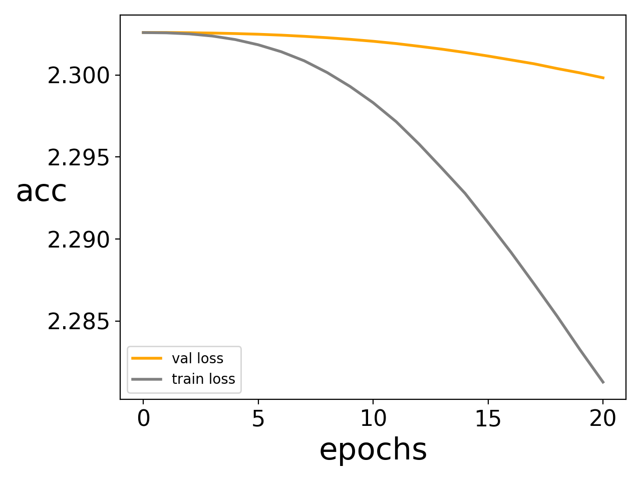
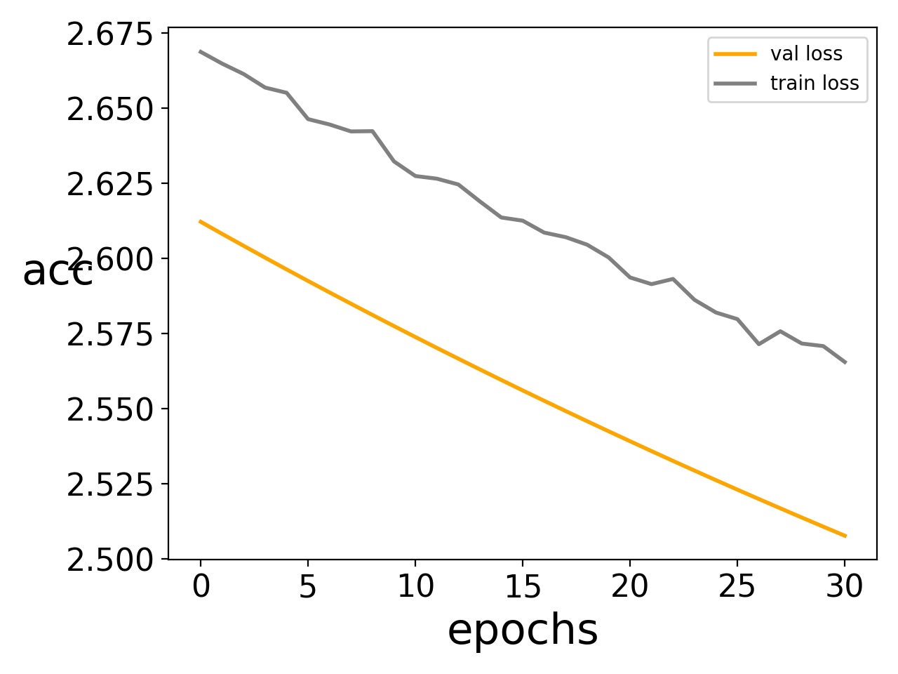
Refer to caption
(a) Fig.2(a) Step 20
Refer to caption
(b) Fig.2(b) Step 30
Refer to caption
(c) Fig.2(c) Step 30
Refer to caption
(d) Fig.2(d) Step 61
Refer to caption
(e) Fig.3(a) Step 100
Refer to caption
(f) Fig.3(b) Step 100
Refer to caption
(g) Fig.3(c) Step 100
Refer to caption
(h) Fig.3(d) Step 100
Refer to caption
(i) Fig.3(e) Step 100
Refer to caption
(j) Fig.4 Step 900 to 1400
Figure 7: Losses from Fig. 2 to Fig.4. The original figures and the numbers of steps corresponding to each sub-picture are written in the sub-captions.
Refer to caption
(a) Fig.5(a) Step 1000
Refer to caption
(b) Fig.5(b) Step 1000
Refer to caption
(c) Fig.5(c) Step 1000
Refer to caption
(d) Fig.5(d) Step 1000
Refer to caption
(e) Fig.6(a) Step 200
Refer to caption
(f) Fig.6(b) Step 200
Refer to caption
(g) Fig.6(c) Step 200
Refer to caption
(h) Fig.6(d) Step 200
Figure 8: Losses from Fig. 5 to Fig.6. The original figures and the numbers of steps corresponding to each sub-picture are written in the sub-captions.

A.4 Performance of tanh activation function in condensed regime

For practical networks, such as resnet18-like (He et al., 2016) in learning CIFAR10, as shown in Fig. 9 and Table 1, we find that the performance of networks with initialization in the condensed regime is vary similar to the common initialization methods. For both initialization methods, the test accuracy is about 86.5%percent\% to 88.5%percent\%, where the highest test accuracy and lowest test accuracy for common methods are 88.07%percent\% and 86.73%percent\%, respectively, while the highest one and lowest one for condensed methods are 88.26%percent\% and 86.88%percent\%, respectively. This implies that performance of common and condensed initialization is similar.
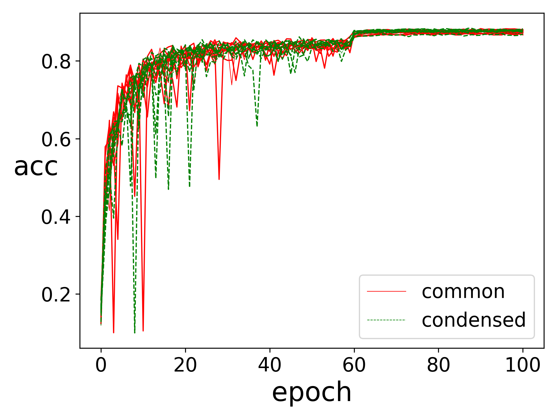
Refer to caption
(a) test accuracy
Figure 9: The test accuracy of Resnet18-like networks with different initialization methods. Each network consists of the convolution part of resnet18 and fully-connected (FC) layers with size 1024-1024-10 and softmax. The convolution part is equipped with ReLU activation and initialized by Glorot normal distribution (Glorot and Bengio, 2010). For FC layers, the activation is tanh(x)𝑥\tanh{(x)} and they are initialized by three common methods (red) and three condensed ones (green) as indicated in Table 1. The learning rate is 103superscript10310^{-3} for epoch 1-60 and 104superscript10410^{-4} for epoch 61-100. Adam optimizer with cross-entropy loss and batch size 128 are used for all experiments.
Table 1: Comparison of test accuracy of resnet18 in learning CIFAR10 with common (Glorot and Bengio, 2010) and condensed Gaussian initializations. m¯=(min+mout)/2¯𝑚subscript𝑚insubscript𝑚out2\bar{m}=(m_{\rm in}+m_{\rm out})/2. minsubscript𝑚inm_{\rm in}: in-layer width. moutsubscript𝑚outm_{\rm out}: out-layer width. Each line is a trial.
common condensed
Glorot_uniform Glorot_normal N(0,1m¯)𝑁01¯𝑚N(0,\frac{1}{\bar{m}}) N(0,1mout4)𝑁01superscriptsubscript𝑚out4N(0,\frac{1}{m_{\rm out}^{4}}) N(0,1mout3)𝑁01superscriptsubscript𝑚out3N(0,\frac{1}{m_{\rm out}^{3}}) N(0,(1m¯)2)𝑁0superscript1¯𝑚2N(0,(\frac{1}{\bar{m}})^{2})
Test 1 0.8747 0.8759 0.8807 0.8749 0.8744 0.8765
Test 2 0.8715 0.8673 0.8733 0.8763 0.8799 0.8826
Test 3 0.8772 0.8794 0.8788 0.8688 0.8780 0.8771

A.5 multi-layer experimental

The condensation of the six layer without residual connections is shown in 10, whose activation functions for hidden layer 1 to hidden layer 5 are x2tanh(x)superscript𝑥2𝑥x^{2}\tanh(x), xtanh(x)𝑥𝑥x\tanh(x), sigmoid(x)sigmoid𝑥\mathrm{sigmoid}(x), tanh(x)𝑥\tanh(x) and softplus(x)softplus𝑥\mathrm{softplus}(x), respectively.

The condensation of the three layer without residual connections is shown in 11, whose activation functions are same for each layer indicated by the corresponding sub-captions.

The condensation of the five layer without residual connections is shown in 12, whose activation functions are same for each layer indicated by the corresponding sub-captions.

The condensation of the five layer with residual connections is shown in 13, whose activation functions are same for each layer indicated by the corresponding sub-captions.
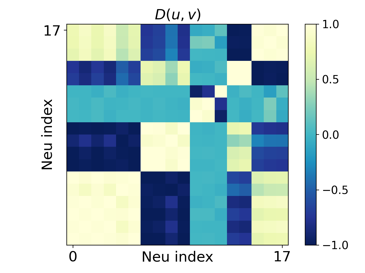
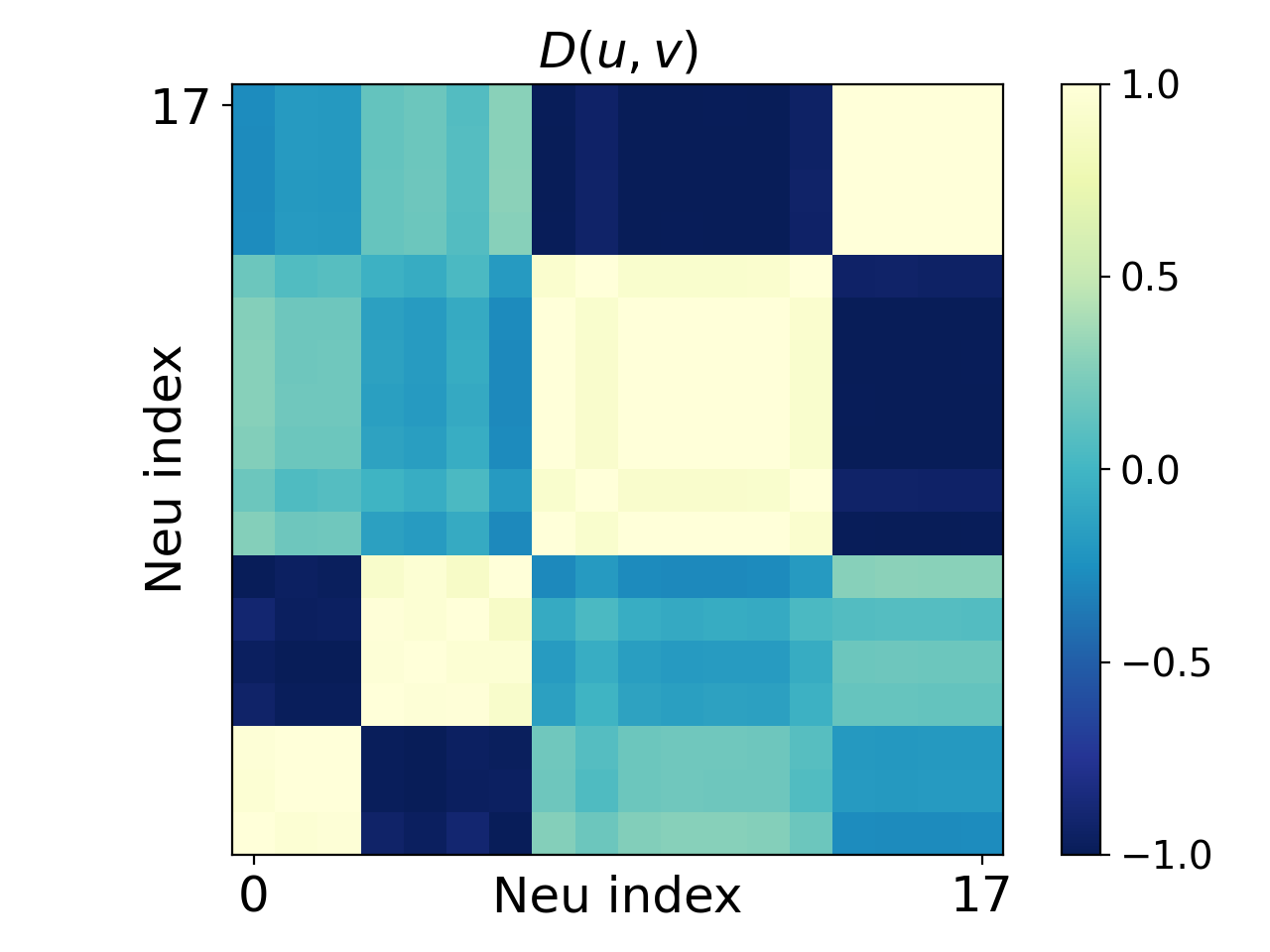
Refer to caption
(a) layer 1
Refer to caption
(b) layer 2
Refer to caption
(c) layer 3
Refer to caption
(d) layer 4
Refer to caption
(e) layer 5
Figure 10: Condensation of six-layer NNs without residual connections. The activation functions for hidden layer 1 to hidden layer 5 are x2tanh(x)superscript𝑥2𝑥x^{2}\tanh(x), xtanh(x)𝑥𝑥x\tanh(x), sigmoid(x)sigmoid𝑥\mathrm{sigmoid}(x), tanh(x)𝑥\tanh(x) and softplus(x)softplus𝑥\mathrm{softplus}(x), respectively.The numbers of steps selected in the sub-pictures are epoch 6800, epoch 6800, epoch 6800, epoch 6800 and epoch 6300, respectively, while the NN is only trained once. The color indicates D(𝒖,𝒗)𝐷𝒖𝒗D(\bm{u},\bm{v}) of two hidden neurons’ input weights, whose indexes are indicated by the abscissa and the ordinate, respectively. The training data is 808080 points sampled from a 3-dimensional function k=134sin(12xk+1)superscriptsubscript𝑘13412subscript𝑥𝑘1\sum_{k=1}^{3}4\sin(12x_{k}+1), where each xksubscript𝑥𝑘x_{k} is uniformly sampled from [4,2]42[-4,2]. n=80𝑛80n=80, d=3𝑑3d=3, m=18𝑚18m=18, dout=1subscript𝑑out1d_{\mathrm{out}}=1, var=0.0082varsuperscript0.0082\mathrm{var}=0.008^{2}, lr=5×10⁵lr5superscript105\mathrm{lr}=5\times 10^{-5}.
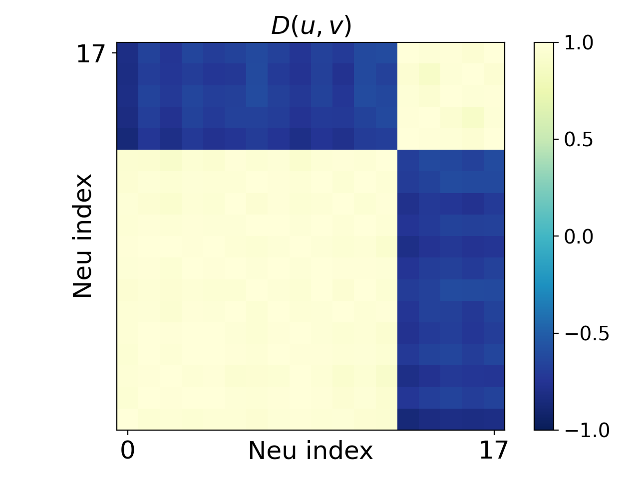
Refer to caption
(a) tanh(x)𝑥\tanh(x)
Refer to caption
(b) xtanh(x)𝑥𝑥x\tanh(x)
Refer to caption
(c) x2tanh(x)superscript𝑥2𝑥x^{2}\tanh(x)
Refer to caption
(d) ReLU(x)ReLU𝑥\mathrm{ReLU}(x)
Refer to caption
(e) sigmoid(x)sigmoid𝑥\mathrm{sigmoid}(x)
Refer to caption
(f) softplus(x)softplus𝑥\mathrm{softplus}(x)
Refer to caption
(g) tanh(x)𝑥\tanh(x)
Refer to caption
(h) xtanh(x)𝑥𝑥x\tanh(x)
Refer to caption
(i) x2tanh(x)superscript𝑥2𝑥x^{2}\tanh(x)
Refer to caption
(j) ReLU(x)ReLU𝑥\mathrm{ReLU}(x)
Refer to caption
(k) sigmoid(x)sigmoid𝑥\mathrm{sigmoid}(x)
Refer to caption
(l) softplus(x)softplus𝑥\mathrm{softplus}(x)
Figure 11: Three-layer NN at epoch 700700700. (a-f) are for the input weights of the first hidden layer and (g-l) are for the input weights of the second hidden layer. The color indicates D(𝒖,𝒗)𝐷𝒖𝒗D(\bm{u},\bm{v}) of two hidden neurons’ input weights, whose indexes are indicated by the abscissa and the ordinate, respectively. The training data is 808080 points sampled from a 5-dimensional function k=153sin(8xk+1)superscriptsubscript𝑘1538subscript𝑥𝑘1\sum_{k=1}^{5}3\sin(8x_{k}+1), where each xksubscript𝑥𝑘x_{k} is uniformly sampled from [4,2]42[-4,2]. n=80𝑛80n=80, d=5𝑑5d=5, m=50𝑚50m=50, dout=1subscript𝑑out1d_{\mathrm{out}}=1, var=0.0052varsuperscript0.0052\mathrm{var}=0.005^{2}. lr=104,2×105,1.4×105lrsuperscript1042superscript1051.4superscript105\mathrm{lr}=10^{-4},2\times 10^{-5},1.4\times 10^{-5} for (a-d), (e) and (f), respectively. For (d) and (j), we discard hidden neurons, whose L2subscript𝐿2L_{2}-norm of its input weight is smaller than 0.10.10.1.
Refer to caption
(a) tanh(x)𝑥\tanh(x)
Refer to caption
(b) tanh(x)𝑥\tanh(x)
Refer to caption
(c) tanh(x)𝑥\tanh(x)
Refer to caption
(d) tanh(x)𝑥\tanh(x)
Refer to caption
(e) xtanh(x)𝑥𝑥x\tanh(x)
Refer to caption
(f) xtanh(x)𝑥𝑥x\tanh(x)
Refer to caption
(g) xtanh(x)𝑥𝑥x\tanh(x)
Refer to caption
(h) xtanh(x)𝑥𝑥x\tanh(x)
Refer to caption
(i) x2tanh(x)superscript𝑥2𝑥x^{2}\tanh(x)
Refer to caption
(j) x2tanh(x)superscript𝑥2𝑥x^{2}\tanh(x)
Refer to caption
(k) x2tanh(x)superscript𝑥2𝑥x^{2}\tanh(x)
Refer to caption
(l) x2tanh(x)superscript𝑥2𝑥x^{2}\tanh(x)
Refer to caption
(m) sigmoid(x)𝑠𝑖𝑔𝑚𝑜𝑖𝑑𝑥sigmoid(x)
Refer to caption
(n) sigmoid(x)𝑠𝑖𝑔𝑚𝑜𝑖𝑑𝑥sigmoid(x)
Refer to caption
(o) sigmoid(x)𝑠𝑖𝑔𝑚𝑜𝑖𝑑𝑥sigmoid(x)
Refer to caption
(p) sigmoid(x)𝑠𝑖𝑔𝑚𝑜𝑖𝑑𝑥sigmoid(x)
Refer to caption
(q) softplus(x)𝑠𝑜𝑓𝑡𝑝𝑙𝑢𝑠𝑥softplus(x)
Refer to caption
(r) softplus(x)𝑠𝑜𝑓𝑡𝑝𝑙𝑢𝑠𝑥softplus(x)
Refer to caption
(s) softplus(x)𝑠𝑜𝑓𝑡𝑝𝑙𝑢𝑠𝑥softplus(x)
Refer to caption
(t) softplus(x)𝑠𝑜𝑓𝑡𝑝𝑙𝑢𝑠𝑥softplus(x)
Figure 12: Five-layer NN. The first to fourth columns of each row are for the input weights of neurons from the first to the fourth hidden layers, respectively. The color indicates D(𝒖,𝒗)𝐷𝒖𝒗D(\bm{u},\bm{v}) of two hidden neurons’ input weights, whose indexes are indicated by the abscissa and the ordinate, respectively. The training data is 808080 points sampled from a 5-dimensional function k=133sin(10xk+1)superscriptsubscript𝑘13310subscript𝑥𝑘1\sum_{k=1}^{3}3\sin(10x_{k}+1), where each xksubscript𝑥𝑘x_{k} is uniformly sampled from [4,2]42[-4,2]. n=80𝑛80n=80, d=5𝑑5d=5, m=18𝑚18m=18, dout=1subscript𝑑out1d_{\mathrm{out}}=1, var=0.0082varsuperscript0.0082\mathrm{var}=0.008^{2}. lr=1.5×10⁵, 1.5×10⁵, 1.5×10⁵, 1.5×10⁵, 1.5×10⁶lr1.5superscript1051.5superscript1051.5superscript1051.5superscript1051.5superscript106\mathrm{lr}=1.5\times 10^{-5},\ 1.5\times 10^{-5},\ 1.5\times 10^{-5},\ 1.5\times 10^{-5},\ 1.5\times 10^{-6} and epoch is 10000, 10000, 26000, 10000, 20000100001000026000100002000010000,\ 10000,\ 26000,\ 10000,\ 20000 for tanh(x)𝑥\tanh(x), xtanh(x)𝑥𝑥x\tanh(x), x2tanh(x)superscript𝑥2𝑥x^{2}\tanh(x), sigmoid(x)𝑠𝑖𝑔𝑚𝑜𝑖𝑑𝑥sigmoid(x), softplus(x)𝑠𝑜𝑓𝑡𝑝𝑙𝑢𝑠𝑥softplus(x), respectively.
Refer to caption
(a) tanh(x)𝑥\tanh(x)
Refer to caption
(b) tanh(x)𝑥\tanh(x)
Refer to caption
(c) tanh(x)𝑥\tanh(x)
Refer to caption
(d) tanh(x)𝑥\tanh(x)
Refer to caption
(e) xtanh(x)𝑥𝑥x\tanh(x)
Refer to caption
(f) xtanh(x)𝑥𝑥x\tanh(x)
Refer to caption
(g) xtanh(x)𝑥𝑥x\tanh(x)
Refer to caption
(h) xtanh(x)𝑥𝑥x\tanh(x)
Refer to caption
(i) x2tanh(x)superscript𝑥2𝑥x^{2}\tanh(x)
Refer to caption
(j) x2tanh(x)superscript𝑥2𝑥x^{2}\tanh(x)
Refer to caption
(k) x2tanh(x)superscript𝑥2𝑥x^{2}\tanh(x)
Refer to caption
(l) x2tanh(x)superscript𝑥2𝑥x^{2}\tanh(x)
Refer to caption
(m) sigmoid(x)𝑠𝑖𝑔𝑚𝑜𝑖𝑑𝑥sigmoid(x)
Refer to caption
(n) sigmoid(x)𝑠𝑖𝑔𝑚𝑜𝑖𝑑𝑥sigmoid(x)
Refer to caption
(o) sigmoid(x)𝑠𝑖𝑔𝑚𝑜𝑖𝑑𝑥sigmoid(x)
Refer to caption
(p) sigmoid(x)𝑠𝑖𝑔𝑚𝑜𝑖𝑑𝑥sigmoid(x)
Refer to caption
(q) softplus(x)𝑠𝑜𝑓𝑡𝑝𝑙𝑢𝑠𝑥softplus(x)
Refer to caption
(r) softplus(x)𝑠𝑜𝑓𝑡𝑝𝑙𝑢𝑠𝑥softplus(x)
Refer to caption
(s) softplus(x)𝑠𝑜𝑓𝑡𝑝𝑙𝑢𝑠𝑥softplus(x)
Refer to caption
(t) softplus(x)𝑠𝑜𝑓𝑡𝑝𝑙𝑢𝑠𝑥softplus(x)
Figure 13: Five-layer NN. The first to fourth columns of each row are for the input weights of neurons from the first to the fourth hidden layers, respectively. The color indicates D(𝒖,𝒗)𝐷𝒖𝒗D(\bm{u},\bm{v}) of two hidden neurons’ input weights, whose indexes are indicated by the abscissa and the ordinate, respectively. The training data is 808080 points sampled from a 5-dimensional function k=133sin(10xk+1)superscriptsubscript𝑘13310subscript𝑥𝑘1\sum_{k=1}^{3}3\sin(10x_{k}+1), where each xksubscript𝑥𝑘x_{k} is uniformly sampled from [4,2]42[-4,2]. n=80𝑛80n=80, d=5𝑑5d=5, m=18𝑚18m=18, dout=1subscript𝑑out1d_{\mathrm{out}}=1, var=0.0082varsuperscript0.0082\mathrm{var}=0.008^{2}. lr=1×10⁴, 1×10⁴, 1×10⁴, 5×10⁵, 5×10⁵lr1superscript1041superscript1041superscript1045superscript1055superscript105\mathrm{lr}=1\times 10^{-4},\ 1\times 10^{-4},\ 1\times 10^{-4},\ 5\times 10^{-5},\ 5\times 10^{-5} and epoch is 400, 400, 400, 3000, 360, 4004004004003000360400400,\ 400,\ 400,\ 3000,\ 360,\ 400 for tanh(x)𝑥\tanh(x), xtanh(x)𝑥𝑥x\tanh(x), x2tanh(x)superscript𝑥2𝑥x^{2}\tanh(x), x2tanh(x)superscript𝑥2𝑡𝑎𝑛𝑥x^{2}tanh(x), sigmoid(x)𝑠𝑖𝑔𝑚𝑜𝑖𝑑𝑥sigmoid(x), softplus(x)𝑠𝑜𝑓𝑡𝑝𝑙𝑢𝑠𝑥softplus(x), respectively.

A.6 Several steps during the evolution of condensation at the initial stage

In the article, we only give the results of the last step of each condense, while the details of the evolution of condensation are lacking, which may provide a better understanding. Therefore, we show these details in Fig. 14, Fig. 15, Fig. 16 and Fig. 17, which also further illustrate the rationality of the experimental results and facilitate the understanding of the evolution of condensation in the initial stage.

Refer to caption
(a) Step 1
Refer to caption
(b) Step 5
Refer to caption
(c) Step 7
Refer to caption
(d) Step 10
Refer to caption
(e) Step 20
Refer to caption
(f) Step 1
Refer to caption
(g) Step 4
Refer to caption
(h) Step 8
Refer to caption
(i) Step 15
Refer to caption
(j) Step 30
Refer to caption
(k) Step 1
Refer to caption
(l) Step 4
Refer to caption
(m) Step 8
Refer to caption
(n) Step 15
Refer to caption
(o) Step 30
Refer to caption
(p) Step 30
Refer to caption
(q) Step 51
Refer to caption
(r) Step 54
Refer to caption
(s) Step 58
Refer to caption
(t) Step 61
Figure 14: Evolution of condensation of Fig. 2(a), Fig. 2(b), Fig. 2(c), and Fig. 2(d). The evolution from the first row to the fourth row are corresponding to the Fig. 2(a), Fig. 2(b), Fig. 2(c), and Fig. 2(d). The numbers of evolutionary steps are shown in the sub-captions, where sub-figures in the last row are the epochs in the article.
Refer to caption
(a) Step 5
Refer to caption
(b) Step 10
Refer to caption
(c) Step 15
Refer to caption
(d) Step 50
Refer to caption
(e) Step 100
Refer to caption
(f) Step 5
Refer to caption
(g) Step 10
Refer to caption
(h) Step 15
Refer to caption
(i) Step 50
Refer to caption
(j) Step 100
Refer to caption
(k) Step 10
Refer to caption
(l) Step 20
Refer to caption
(m) Step 40
Refer to caption
(n) Step 60
Refer to caption
(o) Step 100
Refer to caption
(p) Step 10
Refer to caption
(q) Step 20
Refer to caption
(r) Step 40
Refer to caption
(s) Step 60
Refer to caption
(t) Step 100
Refer to caption
(u) Step 10
Refer to caption
(v) Step 20
Refer to caption
(w) Step 40
Refer to caption
(x) Step 60
Refer to caption
(y) Step 100
Figure 15: Evolution of condensation from Fig. 3(a) to 3(e). The evolution from the first row to the fifth row are corresponding to the Fig. 3(a), Fig. 3(b), Fig. 3(c), Fig. 3(d), Fig. 3(e). The numbers of evolutionary steps are shown in the sub-captions, where sub-figures in the last row are the epochs in the article.
Refer to caption
(a) Step 200
Refer to caption
(b) Step 400
Refer to caption
(c) Step 600
Refer to caption
(d) Step 800
Refer to caption
(e) Step 1000
Refer to caption
(f) Step 200
Refer to caption
(g) Step 400
Refer to caption
(h) Step 600
Refer to caption
(i) Step 800
Refer to caption
(j) Step 900
Refer to caption
(k) Step 100
Refer to caption
(l) Step 200
Refer to caption
(m) Step 600
Refer to caption
(n) Step 800
Refer to caption
(o) Step 900
Refer to caption
(p) Step 300
Refer to caption
(q) Step 600
Refer to caption
(r) Step 800
Refer to caption
(s) Step 1000
Refer to caption
(t) Step 1400
Refer to caption
(u) Step 100
Refer to caption
(v) Step 500
Refer to caption
(w) Step 900
Refer to caption
(x) Step 1000
Refer to caption
(y) Step 1400
Figure 16: Evolution of condensation from Fig. 4(a) to 4(e). The evolution from the first row to the fifth row are corresponding to the Fig. 4(a), Fig. 4(b), Fig. 4(c), Fig. 4(d), Fig. 4(e). The numbers of evolutionary steps are shown in the sub-captions, where sub-figures in the last row are the epochs in the article.
Refer to caption
(a) Step 40
Refer to caption
(b) Step 80
Refer to caption
(c) Step 120
Refer to caption
(d) Step 160
Refer to caption
(e) Step 200
Refer to caption
(f) Step 40
Refer to caption
(g) Step 80
Refer to caption
(h) Step 120
Refer to caption
(i) Step 160
Refer to caption
(j) Step 200
Refer to caption
(k) Step 40
Refer to caption
(l) Step 80
Refer to caption
(m) Step 120
Refer to caption
(n) Step 160
Refer to caption
(o) Step 200
Figure 17: Evolution of condensation from Fig. 6(a) to 6(c). The evolution from the first row to the fifth row are corresponding to the Fig. 6(a), Fig. 6(b), and Fig. 6(c). The numbers of evolutionary steps are shown in the sub-captions, where sub-figures in the last row are the epochs in the article.

A.7 The influence of training data on condensation

We also find that when the training data is less oscillated, the NN may condense at fewer directions. For example, as shown in Fig. 18(a), compared with the high frequency function in Fig. 3, we only change the target function to be a lower-frequency function, i.e., k=153.5sin(2xk+1)superscriptsubscript𝑘153.52subscript𝑥𝑘1\sum_{k=1}^{5}3.5\sin(2x_{k}+1). In this case, the NN with x2tanh(x)superscript𝑥2𝑥x^{2}\tanh(x) only condenses at three directions, in which two are opposite. For MNIST data in Fig. 18(b), we find that, the NN with x2tanh(x)superscript𝑥2𝑥x^{2}\tanh(x) condenses at one line, which may suggest that the function for fitting MNIST dataset is a low-frequency function. For CIFAR100 data in Fig. 18(c), we find that input weights of the first FC layer with xtanh(x)𝑥𝑥x\tanh(x) condense at only one line, which implies that features extracted by the convolution part of the NN may own low complexity.
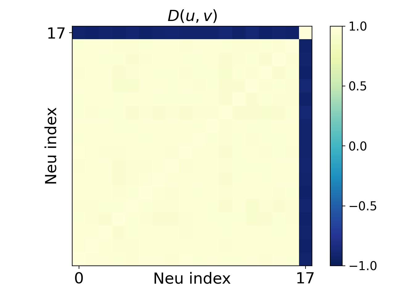
These experiments does not contradict to our results, which claim that the maximal number of condensed orientations in the initial training is twice the multiplicity of the activation function used in general NNs.

For CIFAR100 dataset, we use Resnet18-like neural network, which has been described in Fig. 2. Besides, the input dimension is d=32323𝑑32323d=32*32*3, the output dimension is dout=100subscript𝑑out100d_{\mathrm{out}}=100, and all parameters are initialized by a Gaussian distribution N(0,var)𝑁0varN(0,\mathrm{var}). The total data size is n𝑛n. The training method is Adam with batch size 128, learning rate lrlr\mathrm{lr} and cross-entropy loss.
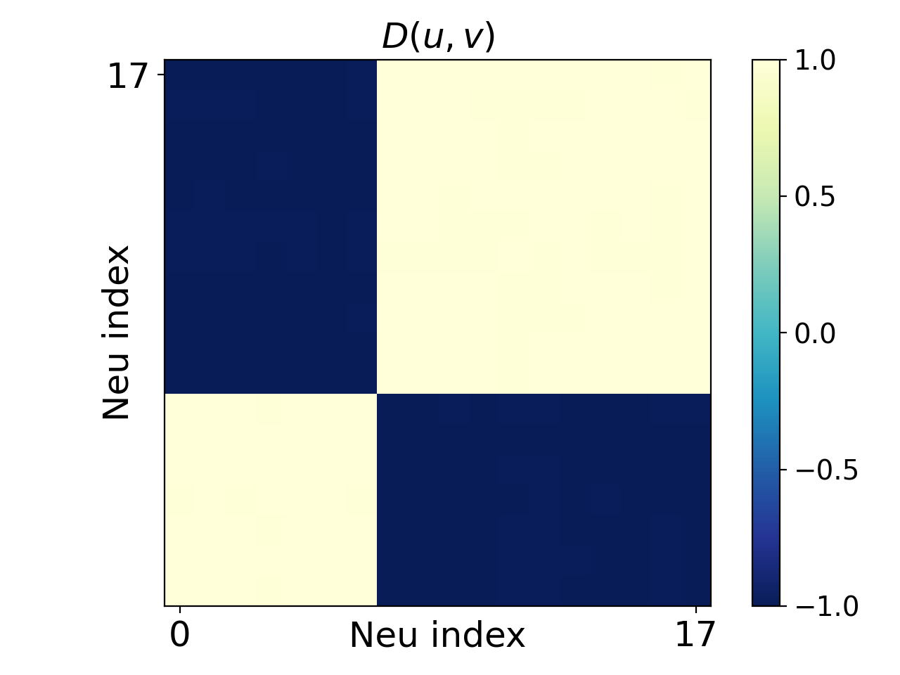
For MNIST dataset, we use fully-connected neural network with size, d𝑑d-m𝑚m-\cdots-m𝑚m-doutsubscript𝑑outd_{\mathrm{out}}. The input dimension is d=784𝑑784d=784, and the output dimension is dout=10subscript𝑑out10d_{\mathrm{out}}=10. The number of hidden neurons m𝑚m is specified in Fig. 18. All parameters are initialized by a Gaussian distribution N(0,var)𝑁0varN(0,\mathrm{var}). The total data size is n𝑛n. The training method is Adam with full batch, learning rate lrlr\mathrm{lr} and MSE loss.

Refer to caption
(a) k=153.5sin(2xk+1)superscriptsubscript𝑘153.52subscript𝑥𝑘1\sum_{k=1}^{5}3.5\sin(2x_{k}+1)
Refer to caption
(b) MNIST
Refer to caption
(c) CIFAR100
Figure 18: Condensation of low-frequency functions with two-layer NNs in (a,b) and condensation of the first FC layer of the Resnet18-like network on CIFAR100 in (c). The color indicates D(𝒖,𝒗)𝐷𝒖𝒗D(\bm{u},\bm{v}) of two hidden neurons’ input weights, whose indexes are indicated by the abscissa and the ordinate. For (a,b), two-layer NN at epoch: 100100100 with activation function: x2tanh(x)superscript𝑥2𝑥x^{2}\tanh(x). For (a), we discard about 15%percent\% of hidden neurons, in which the L2subscript𝐿2L_{2}-norm of each input weight is smaller than 0.040.040.04, while remaining those bigger than 0.40.40.4. The mean magnitude here for each parameter is (0.42/785)0.5 similar-to\sim0.01, which should also be quite small. All settings in (a) are the same as Fig. 3, except for the lower frequency target function. Parameters for (b) are n=60000𝑛60000n=60000, d=784𝑑784d=784, m=30𝑚30m=30, dout=10subscript𝑑out10d_{\mathrm{out}}=10, var=0.0012varsuperscript0.0012\mathrm{var}=0.001^{2}. lr=5×10⁵lr5superscript105\mathrm{lr}=5\times 10^{-5}. The structure and parameters of the Resnet18-like neural network for (c) is the same as Fig. 2, except for the data set CIFAR100 and learning rate lr=1×10⁶lr1superscript106\mathrm{lr}=1\times 10^{-6}.