Bounds on the recurrence probability in periodically -driven quantum systems
Abstract
Periodically-driven systems are ubiquitous in science and technology. In quantum dynamics, even a small number of periodically-driven spins leads to complicated dynamics. Hence, it is of interest to understand what constraints such dynamics must satisfy. We derive a set of constraints for each number of cycles. For pure initial states, the observable being constrained is the recurrence probability. We use our constraints for detecting undesired coupling to unaccounted environments and drifts in the driving parameters. To illustrate the relevance of these results for modern quantum systems we demonstrate our findings experimentally on a trapped-ion quantum computer, and on various IBM quantum computers. Specifically, we provide two experimental examples where these constraints surpass fundamental bounds associated with known one-cycle constraints. This scheme can potentially be used to detect the effect of the environment in quantum circuits that cannot be classically simulated. Finally, we show that, in practice, testing an -cycle constraint requires executing only cycles, which makes the evaluation of constraints associated with hundreds of cycles realistic.
The dynamics of isolated quantum systems become too hard to simulate on a classical computer or solve analytically when more than a few dozen spins are involved. Yet, the unitary evolution that characterizes isolated quantum systems is not arbitrary. It conserves purity, the von Neumann entropy, and any other function that depends on the eigenvalues of the density matrix. However, these conserved quantities are impractical since state tomography or other non-scalable techniques are typically needed to evaluate them. Here we study isolated quantum systems under periodic driving for two reasons. First, to gain a fundamental understanding of how the unitarity of isolated quantum systems restricts the evolution of observables, and second, to show the relevance of these restrictions to noise detection in state-of-the-art quantum computers. We start from the question: is the evolution of observables in a periodically-driven system more restricted compared to non-periodic driving? While is seems intuitively true, to the best of our knowledge no such constraints have been shown. We derive such constraints and show that these inequalities are more restrictive than other known bounds, which do not exploit periodicity. In Sec. 1 we introduce and derive the periodicity inequalities, and in section 2 we experimentally demonstrate their added value by exploring pure and mixed-state scenarios that are challenging for existing bounds as described below.
Constraints on observables that are valid for arbitrary driving have been derived within the frameworks of stochastic and quantum thermodynamics. These constraints include, the second law in quantum microscopic setups fluctuation theorems [1, 2, 3], thermodynamic uncertainty relation [4, 5, 6, 7], passivity based constraints [8, 9, 10], and more. We do not include constraints that involve non-observable, information-like, quantities as in resource theory and other frameworks [10, 11]. As it turns out, thermodynamic constraints loose their predictive power in the zero-temperature limit [12, 13, 14]. In appendix I, we show this explicitly for the second law and the Jarzynski fluctuation theorem. However, in quantum computers and simulators the input state is typically pure, which makes many thermodynamic-based constraints unsuitable for evolution-noise detection. Another challenge for thermodynamic-like constraints involves coherence in the energy basis. Fluctuation theorems, for example, are based on the two-point measurement scheme. The first measurement is carried on the initial state, which leads to wavefunction collapse. Crucially this measurement changes the evolution from a unitary evolution to a mixture of unitaries.
We show the added value of our inequalities by: i) demonstrating that
the periodicity bounds can detect violation of periodicity even if
the system is isolated; ii) showing that the periodicity constraints
remains useful for detecting unaccounted coupling to an environment,
in the zero-temperature temperature limit; iii) breaking a recently
derived bound on the maximal temperature of detectable environments.
Preliminaries: A Simple Inequality For Unitary Evolution
Let be the density matrix that is obtained from by unitary transformation. Due to the non-negativity of the L2 norm it holds that,
Next, we expand this expression and use the cyclic property of the trace to obtain the following form
| (1) |
Since the evolution is unitary,is unitary,the purity is conserved, , and we obtain
| (2) |
Next, we use the fact that for unitary evolution purity conservation can be generalized to any trace value where is the identity operator and is any real number. The proof follows trivially by expending the parentheses. Thus, if is some Hermitian operator (potentially traceless) and evolves unitarily to , i.e. where is a unitary matrix, then by repeating the steps that lead to (2) together with we obtain
| (3) |
1 Periodicity inequalities
1.1 The two-cycle inequality
Next, we consider a periodically-driven system, i.e. the density matrix after each cycle satisfies
| (4) |
where is a unitary evolution operator. The fact that does not depend on reflects the assumption of periodic driving. From linearity, it follows that the object
| (5) |
where and is the density matrix after j cycles, also satisfies . In the following, we use the term ‘stencil’ for . According to (3) it holds that
| (6) |
where .Consider the simple case where , and , the inequality (6) leads to
| (7) | |||||
is the key quantity in our work and we shall refer to it as the recurrence probability. For a pure state, is the projector on to the initial state, . Therefore, is the probability to measure the system in the initial state after cycles. is an inner product, and can therefore be thought of as the amount of overlap with the initial state even for mixed . That is, still expresses to what extent the density matrix returns to its initial value after cycles.
Using purity conservation in unitary evolution, , it holds that
| (8) |
However, is presently in an inconvenient form as both and are unknown. To overcome this we use the fact that the driving is periodic,
| (9) | |||||
Applying eq. (9) in eq. (8) we get
| (10) |
which is the simplest inequality in our approach since it contains only two cycles, or three time points including the initial state. Periodicity was assumed for the driving and the density matrix does not evolve periodically in the general case. Note that the coefficients in (10) sum up to zero. When the evolution is the identity operator,so that , this property leads to a saturation of the inequality 10 of the form .
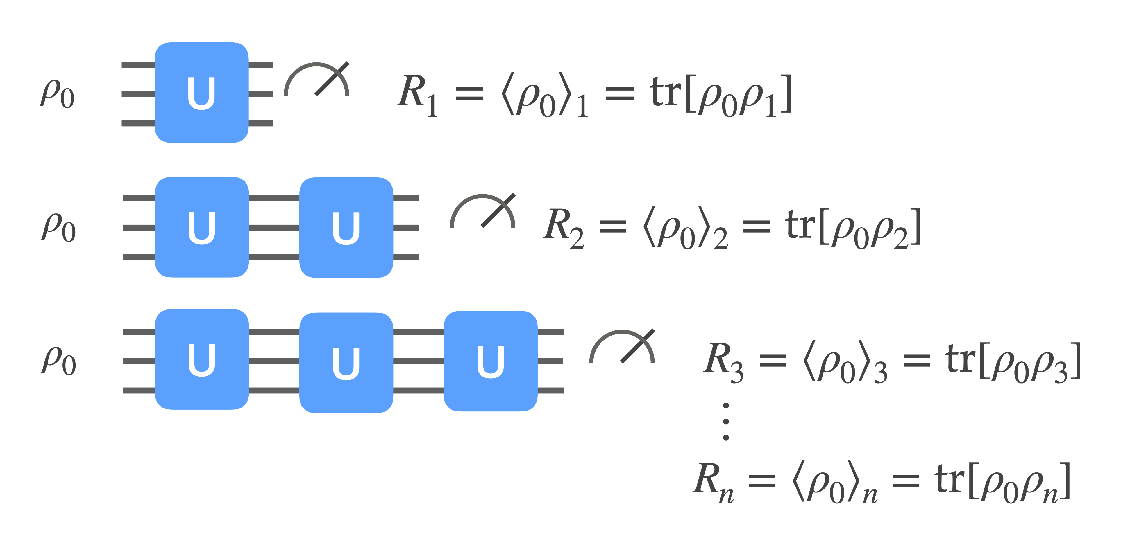
Operationally, the inequality in (10) is evaluated as illustrated in Fig. 1. The measurement can be skipped if the state preparation and measurement errors (SPAM) are negligible. After the initial state is evolved for one cycle, is measured. Next, in a third set of measurements, is measured, and so on.
Note that the one-cycle inequality becomes trivial for pure states since and always holds as the recurrence probability cannot exceed one. In contrast, (10) provides a non-trivial prediction for pure , which is a typical starting point for quantum devices. In Appendix II, we further discuss the two-cycle inequality and its added value for mixed states.
1.2 A recipe for constructing multi-cycle inequalities
The following recipe can be used to obtain more general periodicity bounds:
-
•
Choose a stencil of the form ( are real numbers).
-
•
Choose to set the shift value in .
-
•
Expand the parenthesis in .
-
•
Replace .
The last stage includes the case: . The number of cycles is determinied by largest index of that appears in . Thus the number of cycles in the resulting inequality is .
1.3 The discrete derivative inequalities
The two-cycle inequality (10) was obtained by using the stencil which has the form of a first-order discrete time derivative. Next, we exploit higher-order discrete derivative to generate additional stencils. We denote by the shifted discrete derivative The second derivative is centered at , The third derivative is centered at and so on. This shift ensures that the derivative does not include negative indices. For we choose . Applying the recipe in Sec. (1.2) to the stencils , and denoting the resulting inequalities by where is the number of cycles, the first few inequalities are
| (11) | |||
| (12) | |||
| (13) |
The inequalities can be written as where the coefficients alternate sign as a function of and satisfy and . As shown later, when is sufficiently large the coefficients take the form: .
1.4 Low-cost evaluation of the periodicity inequalities
We introduce the notation , and show in Appendix III that the inequalities can be written as
| (14) |
The expression describes a classical -step random walk with probability to move one step forward, to move one step backward, and to stay in place. For large , the probability distribution for moving moving steps forward is given by the normal distribution with single-step variance :
| (15) |
where we have used: . Applying this result to eq. (14) we find
Expression (LABEL:eq:_Sn_gaussian) suggests that the coefficients decay very fast as a function of and therefore the series can potentially be truncated at some value without significantly changing the value of . Operationally, it means that fewer than cycles are needed for evaluating . This is a useful feature for detecting small evolution noise, that may require evaluating with large .
Next, we set a bound on the error incurred by truncating the sum at .
| (17) | |||||
For convenience we set and get
| (18) |
From (LABEL:eq:_Sn_gaussian) and (18) we finally obtain that the -cycle truncated version of the satisfies
| (19) | |||||
This inequality should be used as follows: is fixed by the that needs to be evaluated, the required accuracy is used to determine via and finally, the truncation value is . For example, to get an error of in the calculation of ( cycles), only cycles need to be measured (). For an accuracy of , cycles are needed (), and measured cycles already yield an accuracy of . We emphasize that in practice the accuracy is limited by statistical noise. For example in the experiment in section 2.3 the truncation error is of the -width when taking points (). For points (), the truncation error is already of the width.
1.5 Optimized three-cycle inequality
In the following, we explore the continuum of three-cycle inequalities, i.e. we are not using the discrete derivative stencil as in the previous sections. The goal is produce bounds that can perform better at detecting evolution noise. Consider the general three-cycle stencil,
| (20) |
where and can take any real value. Using the recipe in Sec. 1.2 we get the following inequality:
| (21) | |||||
We notice that the left hand side, which we denote by , is a second-order polynomial in and , where the coefficients of depend on .
If the evolution is unitary and periodic, for any value of and . Yet, in the presence of evolution noise, might be positive for some choices of and and negative for other choices. It is also possible that is not negative for any choice of and . In that case, the evolution noise is not detectable with four-point periodicity inequalities. To test if the noise is detectable we check if by finding the optimal and that minimize L.
In a given physical scenario that consists of an initial condition and a driving protocol, are just constant positive numbers and is a second-order polynomial with known and fixed coefficients. Next we check which type of paraboloid is. Evaluating the second-derivative test for a paraboloid , we find . If it means that is hyperbolic paraboloid and for some value of it must be negative. implies detection, but this is not surprising since the noise is already detectable with two cycles since . corresponds to , . The more interesting case is where is a paraboloid. Now detection is not guaranteed. Furthermore, the motivation for using an optimized bound for evolution noise detection is that and , which use , failed to detect it. To determine if is a convex or concave paraboloid we check the limit . Since is positive in this limit we conclude is convex. Consequently, the most negative value of occurs when and , we denote the solution to these two equations by and . Finding we get that is equal to
| (22) |
This bound is non-linear in the expectation values since these expectation values are being used to choose the optimal and for detection. If the inequalities that involve and hold, i.e. and , then the non-linear bound (22) simplifies to
| (23) |
The non-linearity in this inequality is different from the density matrix non-linearity that is usually considered in quantum information and quantum thermodynamics (e.g. purity, von Neumann entropy , etc.) as here it appears outside the trace. An experimental measurement of this inequality is given in Sec. 2.4.
While optimized bounds become more burdensome to derive as the number of cycles increases, the existence of these bounds can enable the detection of violations with a relatively small number of measurements.
2 Numerical and Experimental demonstrations
We present numerical simulations and experimental results from IBM superconducting quantum processors and a trapped ion quantum computer (TIQC). Each example illustrates a different feature of the new bounds.
2.1 Detecting parameter drift during the evolution
There are only two assumptions made in deriving the periodicity inequalities, unitarity and periodic driving. A violation of the periodicity inequalities can arise from breaking either one or both of these assumptions. In this section we confirm that a non-periodic shift in the control parameters would manifest as a violation of these bounds by numerically investigating such a possibility.
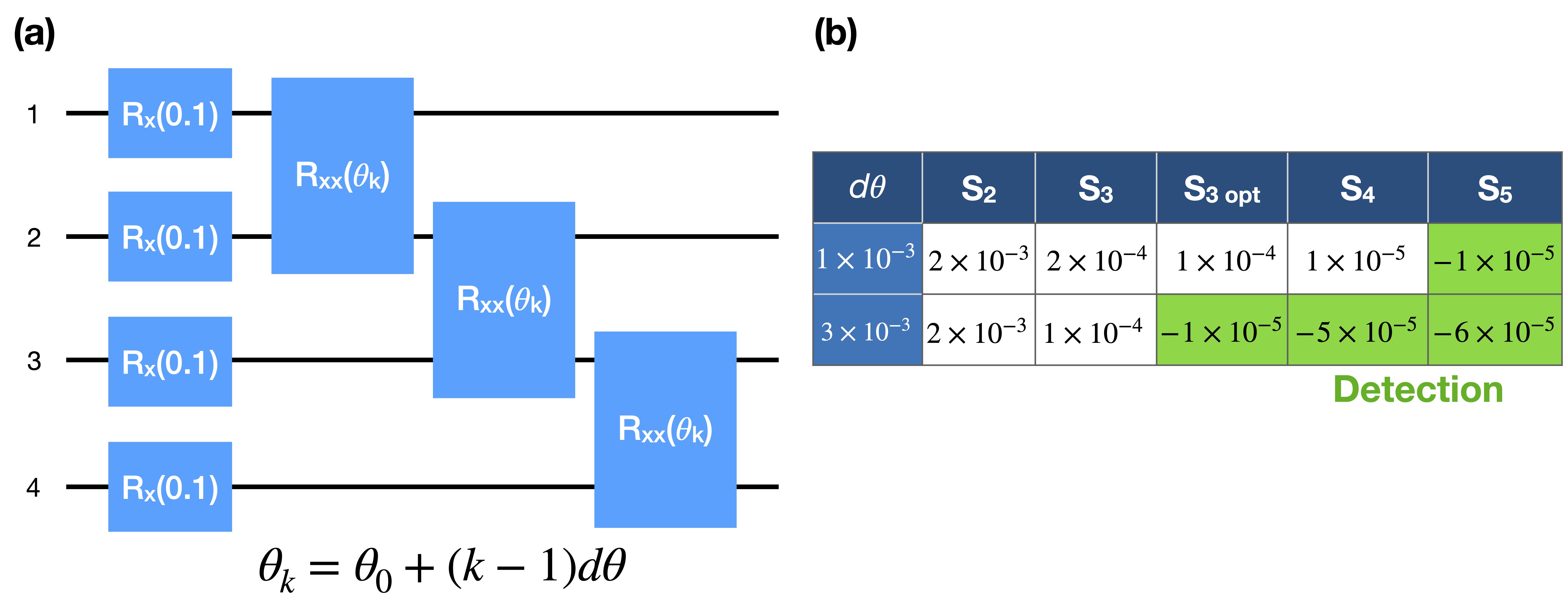
In Fig. 2a we numerically study a four-qubit system where the driving cycle is composed of four single-qubit rotations around the x-axis by angle of 0.1rad where is a single qubit rotation around the x-axis of the Bloch sphere. These rotations are followed by nearest neighbor interactions between qubit and qubit that leads to the following evolution: . In order to simulate a drift of the control parameters, we chose . represents the drift of the parameter from one cycle to the next. The circuit is repeated for up to five cycles. Choosing rad and , the first violation is observed after five cycles where . If the drift is stronger, for example such that , the first violation is observed after three cycles when employing the three-cycle optimized inequality (23), which yields the value . The unoptimized three cycle bound yields Alternatively, an additional cycle can be used to detect the drift without resorting to an optimized bound . Other values appear in Fig. 2b.
The violation of the periodicity inequality shown in this example highlights the power of these inequalities over thermodynamic bounds, which could only detect errors arising from non-unitarity. In this case, we detect the drift error in the device by exploiting tighter bounds arising from the periodicity of the intended evolution.
2.2 Evolution noise detection with a pure initial state
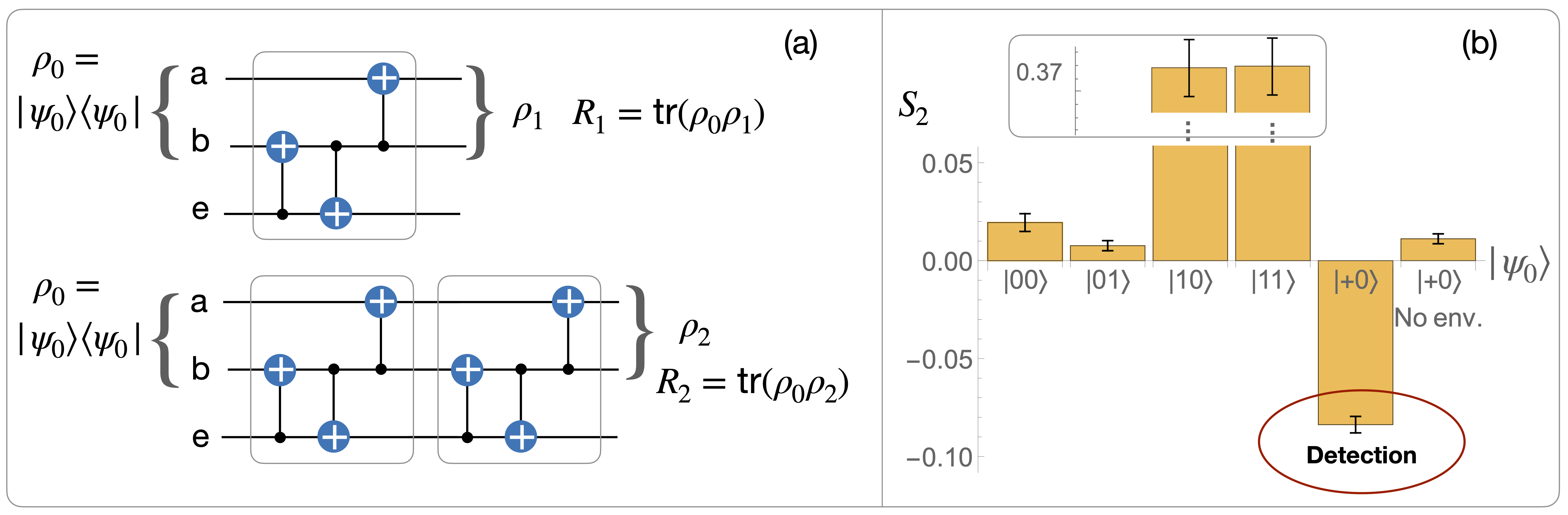
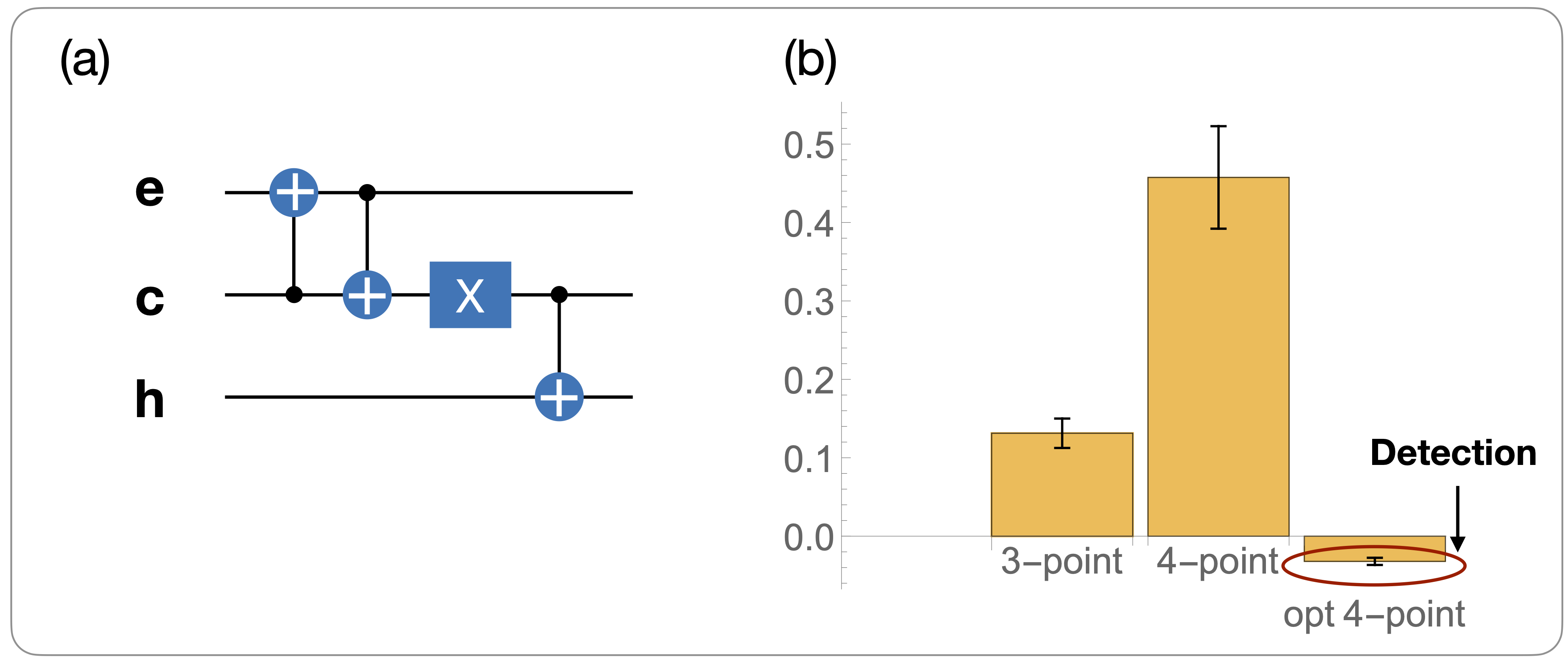
In some setups, such as digital quantum computers, pure-state initial conditions are more natural to use compared to mixed states, which require some dedicated preparation protocol (e.g. see [15] and [16]). It is natural, then, to ask if pure states can be used to detect evolution noise. Presently, constraints on observables in unitary dynamics are derived within the frameworks of stochastic and quantum thermodynamics. Thus, they are the relevant reference for the periodicity inequalities we present. Unfortunately, thermodynamic constraints become impractical to use when the initial state is sufficiently pure. As discussed in Appendix I, some thermodynamic inequalities become so loose that no evolution noise can violate them. In other thermodynamic constraints, the resources needed for evaluating and measuring them diverge as the initial state becomes pure. Hence, thermodynamic constraints are presently not suitable for detecting evolution noise in quantum computers and simulators. The periodicity inequalities studied here are free from this limitation. We present a proof-of-principle experiment for evolution noise detection using pure states. Our setup, shown in Figure 3(a), is composed of a two-qubit system coupled to a one-qubit environment (’e’). The initial state is created by single-qubit gates, which are not shown in the figure. The single cnot gate between the upper two qubits constitutes the periodic unitary driving. While this environment is artificial, it has the advantage that we can easily decouple it from the system and verify that there is no noise detection in this case.
The experiment is composed of three sub-experiments for measuring and . We test several different input states: , and . Our goal is to observe a violation of when the environment is connected, and no violation when it is not. Figure 3(b) shows that states in the computational basis cannot detect the evolution noise but the superposition state in the computation basis can. The error bars correspond to statistical uncertainty. The last bar in Figure 3(b) shows that, as expected, when the environment qubit is decoupled is positive and there is no detection. That is, we confirm that our inequality does not always yield negative values regardless of the coupling to the environment qubit.
Interestingly, the circuit is completely classical for binary input, i.e. diagonal states in the computational basis. In this case, it acts as a simple permutation in the computation basis . The positive values for all four elements of the computation basis [Fig. 3(b)] imply that no classical binary input (including stochastic inputs with classical correlations) can be used to detect the noise induced by the environment qubit ’e’, in this circuit. Yet, a quantum superposition of two classical binary states can detect the coupling to the environment. While this example does not involve a strong quantum feature, such as entanglement, it naturally raises the question if entangled states can lead to detection of noise that cannot be detected using classically-correlated states. The key point of this experiment is the demonstration of noise detection using a unitary constraint when starting in a pure state. A task that, to the best of our knowledge, is not possible using the known thermodynamic constraints.
To conclude this section we point out that while a violation indicates a deviation from a perfect periodic unitary driving, isolating the cause such as parameter drift, decoherence, spontaneous emission, or other evolution noise mechanisms, requires further tests.
2.3 Detection of realistic noise
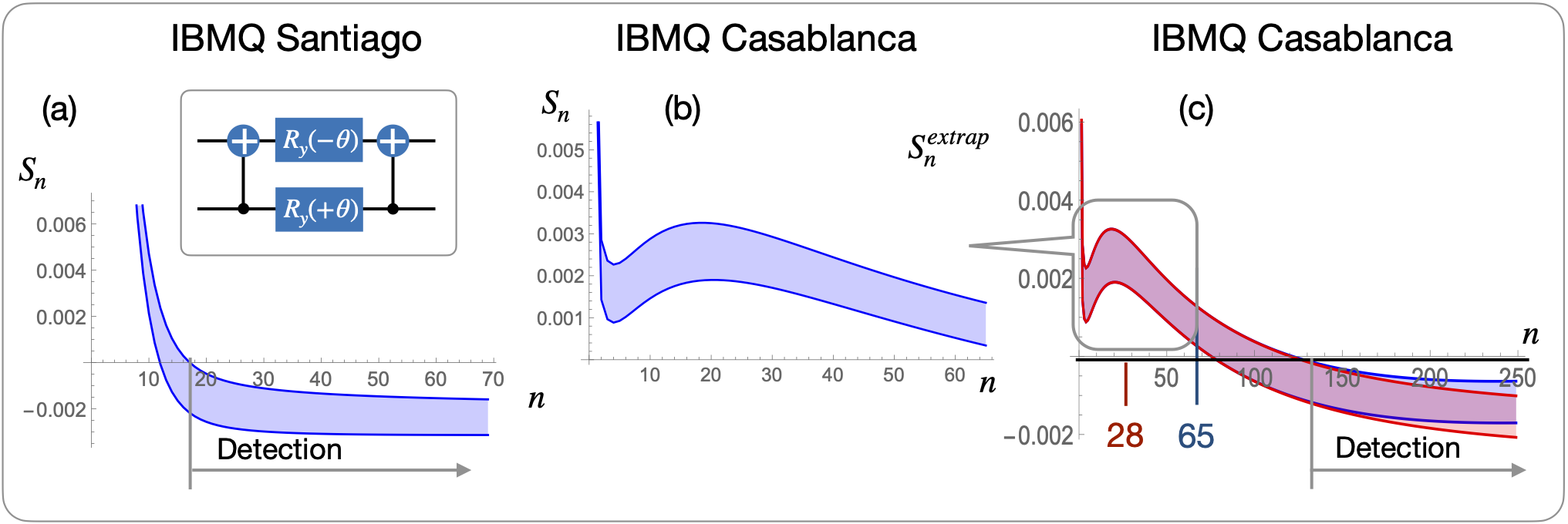
Following the controlled artificial environment demonstration above, it is interesting to check whether this method can detect the real physical environment of quantum processors. The following experiment shows that the real environment is indeed detectable when exploring larger numbers of cycles. The one-cycle circuit we use is shown in the inset of Fig. 4 where . The value of was chosen arbitrarily and it is not optimal. Other values might detect weaker evolution noise or to observe a violation with fewer cycles. Qubits 1 and 2 of the IBM Santiago processor are initialized in the state . Figure 4(a) shows the values of as a function of the number of cycles. The width of the line corresponds uncertainty. Hence, starting from cycles, one can see a violation beyond the 3 uncertainty. This result shows that these inequalities can detect the intrinsic processor noise when using a pure state as the input state.
Figure 4b shows the results of a similar experiment carried out on the IBM Casablanca processor, for 65 cycles and . The value of was modified from the previous experiment as we now wish to demonstrate the utility of the scaling feature presented in Sec. 1.4. In this case, there is no violation within the number of cycles measured, but it seems that if more cycles were measured a violation could have been observed. Fortunately, from the analysis in Sec. 1.4 we know that for large enough the contribution of the last cycles decays like a gaussian in the number of cycles . Consequently, only the first terms contribute to the value of . is roughly 3 but its exact value depends on the required accuracy of the clipped sum with respect to the full sum. This suggests the cycles we have measured can be used to evaluate with . Setting and , we can extrapolate up to with an error of , which is not observable on the scale of Fig 4c. The blue curve, which overlaps with the red curve until , is generated by taking the measured and setting for in the expression for . We find negative values that indicate the presence of evolution noise starting from . We conclude that the noise is detectable with only cycles. This illustrates the efficiency of the inequalities.
It seems that perhaps even samples are more than enough for observing the violation. The red curve is with data from only cycles. The red band shows extrapolation based on only points. According to eq. (18) at cycles, for example, the error should be smaller than , which is too big to confirm a violation. Yet, in practice, at the extrapolation based on points is almost indistinguishable from the one exploiting points. The bound given in eq. (18) on the truncation error of is rather loose since it assumes that the signs of the coefficients do not alternate as a function of , and that all recurrence probabilities are one. Thus, in practice, the contribution of the terms with high cycle number to the sum can be much smaller. In general, it is possible to start with a small number of cycles, and then add more cycles until convergence is achieved at the extrapolated point. Potentially, other initial states can lead to earlier detection of evolution noise, but the goal of this example is to illustrate the advantage of the scaling and not to find the optimal detection scheme.
2.4 Noise Detection Beyond the Hot-Environment Limit
Evolution noise created by hot environments deserves special attention. In the extreme case where the environment is fully mixed, i.e. infinite temperature, the observed system experiences unital dynamics. Unital maps are characterized by the fact that the fully-mixed state is a fixed point of these maps [17, 18]. Decoherence processes are another example of unital map. For practical purposes, it is enough that the temperature is significantly larger than the energies of the system. Although not unitary, unital dynamics are consistent with second-law-like inequalities [19, 20, 14] and passivity-based inequalities [21, 8, 9]. Thus, unital dynamics cannot violate these inequalities, and therefore these inequalities cannot be used to detect unital noise. One can expect that if the environment is slightly less hot so that the system thermalizes to a state, which slightly deviates from a fully mixed state, it will still be hard to detect the noise this environment induces on the system. In Ref. [9] a theorem was derived on the environment temperature that can still be detected: there is no observable in the Hilbert space of the system that satisfies
| (24) |
for any unitary or unital transformation, that can yield , i.e. be violated, when the system is coupled to temperature where
| (25) |
are the energy levels of the environment, and is the -th eigenvalue of (sorted in an increasing order of their size). Hence, if the temperature of the environment exceeds , it is undetectable by inequalities of the form (24). However, this bound is based on the one-cycle scheme with just one final state, in contrast to the multi-cycle approach presented in this paper. Thus, the periodicity inequalities have the potential to detect this type of environment. In the following experiment, we use the circuits shown in Figure 5(a). To generate thermal qubits for the environment and the system, an ensemble of pure states is used (see [15]). The inverse temperatures , and are chosen so that the condition given in eq. (25) guarantees that the environment is too hot to be detected using one-cycle inequalities on observables. As indicated by the negative value of the 3rd bar in Figure 5(b), by evaluating the optimized three-cycle inequality (23) the heat leak becomes detectable.
In summary, this experiment illustrates another added value of the periodicity inequalities with respect to similar inequalities, and that the optimized 3-cycle bound can detect environments that the cannot detect, although both of them use the same experimental data.
2.5 A three-qubit gate in trapped ions and superconducting circuits
Next, we explore the results of for some common gates with simple outputs and consider the regime in which these results would provide benefit as diagnostic. Consider a gate such as cnot, Toffoli (ccnot), Fredkin (cswap), etc. that satisfies i.e. is a two-state permutation so that is the identity operator. If the initial condition is or , the ideal output is . As a result . When the predicted is so simple, there are many ways to quantify the deviation of the device from its expected behavior. For example, one can use. However, this quantity is always positive and a large value of can appear due to coherent error, e.g. miscalibrated gates that change the intended unitary. Thus, may not be associated with noise created by an environment. In contrast, negative values of are a clear indication of evolution noise.
In our last experiment, we run sequentially the Toffoli gate with the initial state where and are the controlling qubits. The experiment is carried out both on the IBMQ superconducting processors and on a TIQC. The TIQC results are obtained on the University of Maryland Trapped Ion (UMDTI) quantum computer, which is described in [22]. This experiment is performed using a linear chain of five ions in a room-temperature Paul trap under ultrahigh vacuum with the qubit encoded in two hyperfine ground states of . We re-analyze raw data from results reported in [23], where three of the five ions are treated as qubits while the others remain idle. For more information on the UMDTI hardware, see Appendix IV.
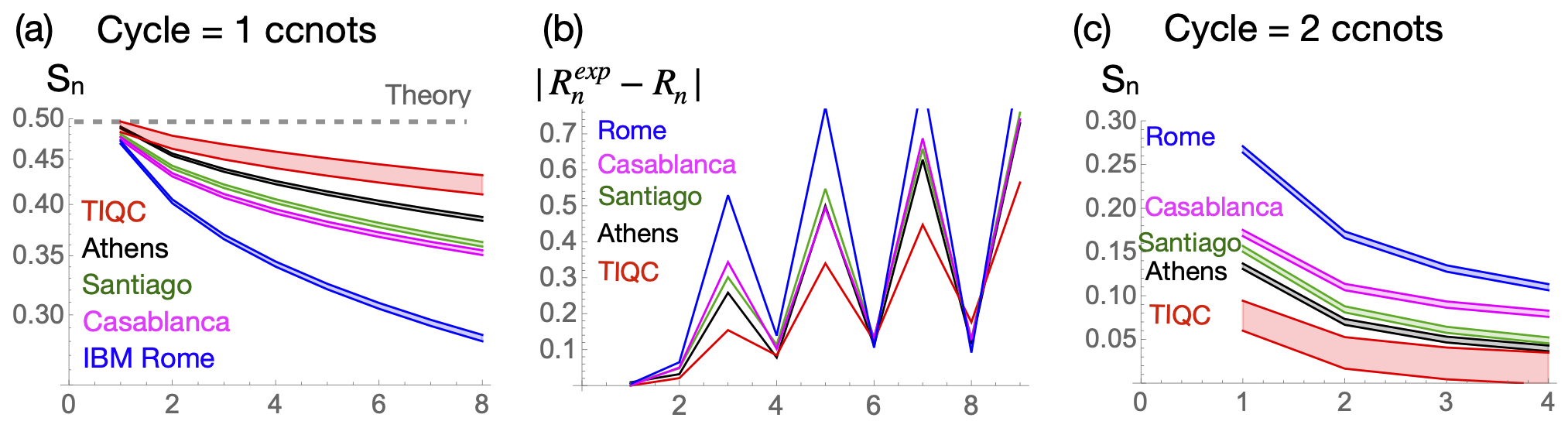
Figure 6(a) shows the plots for various IBM processors and the UMDTI as a function of the number of cycles . The deviation with respect to the ideal output is depicted in Figure 6(b). While the fluctuates, the curves are monotonically decreasing. Using tools that are beyond the present paper one can prove that the series must monotonically decrease if the evolution is unitary and periodic [24, 25]. On the other hand, the fluctuations of and other measures, which are based on distance from the expected output, may be artificial. For example, if the noise is caused by spontaneous emission, the initial state is an excited state, and the ideal recurrence probabilities are , then for odd values, the noise will decrease as it will take the system closer to the ground state and reduce the overlap with the initial excited state. Note that the deviation from in Figure 6(b) can arise from a coherent error in the implementation. It appears that the TIQC data is the closest to the predicted value. Thus, an increase in the plot is an indication for evolution noise, which is not observed here.
In our next test, we group pairs of Toffoli gates as a single cycle. The recurrence probability for this two-Toffoli cycle is . Since it follows that for an ideal evolution for all n. Figure 6(c), shows the experimental values of for the various quantum processors. The same trends as in Figure 6a are observed. Note that in 6(b) Casablanca is more noisy for n=3 and n=7 but it is the other way around for n=5. We conjecture that the reason there are strong fluctuations in and even lack of consistency regarding which processor is more noisy is related to coherent errors. These findings indicate that it is advantageous to check the performance of devices in terms of when the ideal values of are 1,0,1,0,… or 1,1,1,1,… compare to direct evaluation of the individual values, i.e. .
Concluding remarks
We have presented a set of multi-cycle inequalities valid for periodically-driven quantum systems. Presently, we do not claim that these bounds will mature into a practical method for diagnosing evolution noise in quantum circuits, but our results present a clear case that this research direction warrants further investigation. The goal of this paper is to show that it is possible to formulate constraints that are customized to periodic driving and that they have an added value with respect to other known constraints. The periodicity inequalities have three appealing features. The first is the operational advantage: they use pure states and only the recurrence probability is measured. The second is that they treat the circuits as black boxes. The third is the scaling law, which states that only the first cycles contribute to the inequality.
The construction of has additional potential beyond the inequalities studied in this paper. For example, we have shown it is directly related to purity loss and therefore may have further application beyond detecting evolution noise, e.g. for devising a simple protocol for entanglement entropy measurement [24, 25].
Going beyond digital quantum circuits, our method could find applications in other scenarios with periodic driving, such as the simulation of Floquet many-body systems which have applications in the study of time crystals [26] and prethermalization [27]. Typical experimental sequences allow the calculation of bound violations based on existing data, e.g. in [28].
R.U. is grateful for support from Israel Science Foundation (Grant No. 2556/20). A.M.G. is supported by a JQI Postdoctoral Fellowship. N.M.L. acknowledges financial support from NSF grant no. PHY-1430094 to the PFC@JQI, and the Maryland-ARL Quantum Partnership, grant no. W911NF1920181.
Appendix I - The Zero Temperature Problem in Thermodynamic Constraints
There is a broad family of thermodynamic and thermodynamically-inspired constraints. Reviewing how exactly the zero temperature problem manifests in each one is beyond the scope of the present paper. In this appendix, we give as examples the Jarzynski fluctuation theorem, the second law in microscopic quantum systems, and passivity-based inequalities. he Jarzynski equality in systems whose Hamiltonian returns to its initial value reads
where is the transition probability generated by the unitary driving, and is the work invested in creating this transition. It is tempting to ignore all input states save the ground state, which is solely occupied in the limit, however, the exponentially small probabilities are multiplied by an exponentially large factor (e.g. in the transition to the ground state from some other input state). Thus, all input states are important in the ultra-cold limit. This manifests in an exponentially diverging number of shots [13]
which makes this scheme impractical for pure-state initial conditions.
The second law in microscopic systems and passivity inequalities
For an isolated system that starts in thermal equilibrium the relevant statement of the second law is: energy cannot be extracted by applying a periodic force on the system. The translation to quantum systems is as follows: given a time independent system Hamiltonian the initial density of the system is the Gibbs state
| (26) |
where is the inverse temperature. A periodic driving force refers to a periodic driving Hamiltonian that satisfies where is the end of the process. The accumulated effect of the time dependent Hamiltonian can be described by a unitary evolution operator, such that the final density matrix is . The second law in the case states that the final average energy of the bare Hamiltonian is equal to or larger than that of the initial state,
| (27) |
This result can be derived in several ways. In particular, it is a special case of the Clausius-like inequalities for small quantum systems ([14] and references therein).
When is finite this statement is not trivial because the excited states are populated according to (26). Thus, the system can be reduce its energy by moving population to lower states. However, it turns out the unitary transformation (created by the periodic driving) cannot do that. Non-unitary dynamics, such as cooling can reduce the energy but this always involves heating up some other object. Thus, an experimental violation of (27) can be used to deduce that the system is not sufficiently isolated and interaction with an unaccounted environment takes place.
The key point in the context of this paper is that when , i.e. the ultra-cold limit, for all practical purposes only the ground state is initially populated. In this case, it does not matter if the dynamics are unitary or not, and if more objects are involved. The system is already in the minimum possible energy and therefore it can only increase. Since (27) cannot be violated in this case, it cannot be used to detect an environment.
A similar problem exists in passivity-based frameworks. In these framework the basic inequality stems from the passivity of the operator , where is the initial state and is a monotonically-decreasing function in . When , and therefore the basic passivity inequality
becomes trivially satisfied for pure states since (up to a multiplicative positive constant) for any , and the passivity prediction is
which always holds even if the evolution is not unitary. Thus it cannot be used to detect non-unitary environments.
Appendix II - The Two-Cycle Inequality
As a basis for comparison, the usual one-cycle inequality, eq. (2), yields and which for pure states is trivial since and . The inequality (10) can be assigned with different interpretations via different rearrangements:
| (28) | |||
| (29) | |||
| (30) |
Inequality (28) provides a lower bound on (the two-point bound yields an upper bound ), while (29) offers a refined upper bound on . Since this bound is always tighter than the two-point bound . Interestingly this bound is using the information on , so the two endpoints are used for bounding the midpoint. Inequality (30) compares the change in the recurrence probability in the first half to the cumulative change . It suggests that the change cannot occur just in the second half of the evolution; at least a quarter must take place in the first half. Similarly one can write and directly compare the two halves. Note however that in this form the right-hand side might become negative. Another added value of the form (30) is that it makes it easier to compare with the two-point inequalities and . The inequality (30) shows that is not just non-negative but also larger than another non-negative number, . Thus, it is tighter than the two-point prediction .
Appendix III - Derivation of Equation (14)
The n-th discrete shifted derivative can be written where and . Note, that and commute. Using this notation can written as
| (31) |
Next, we use the shift invariance property to obtain
| (32) |
or
| (33) |
Next, we apply the hermitian conjugate of the expression inside the trace. It still gives since it is real but changes to and vice versa and we get the alternative expression
| (34) |
| (35) |
Finally, since we get eq. (14)
Appendix IV - The University of Maryland Trapped-Ion Quantum Computer
The UMDTI quantum computer is described in [22]. Briefly, two-photon Raman transitions are used to control the qubit state, encoded in two magnetic-field-insensitive hyperfine ground states of ions held in a linear chain in a Paul trap. Individual manipulation of each qubit is performed by splitting one of the Raman laser beams into several beams, each controlled by an independent acousto-optic modulator channel and focused onto a single ion in the chain. Single-qubit gate operations are executed by creating laser pulses of controlled phase and duration while two-qubit gates are compiled from single-qubit gates and a laser-driven entangling Ising gate (XX or ) following the Mølmer-Sørensen gate scheme [29, 30, 31], which creates entanglement between pairs of qubits via the shared harmonic oscillator modes of the ion chain in the trap. These modes act as an information bus with which the qubits are temporarily entangled. Modulation of the Raman beam amplitude is used to leave the qubits disentangled from these motional degrees of freedom at the end of the gate operation [32, 33].
References
- Harris and Schütz [2007] Rosemary J Harris and Gunther M Schütz. Fluctuation theorems for stochastic dynamics. Journal of Statistical Mechanics: Theory and Experiment, 2007(07):P07020, 2007. doi: 10.1088/1742-5468/2007/07/P07020. URL https://doi.org/10.1088/1742-5468/2007/07/P07020.
- Seifert [2012] Udo Seifert. Stochastic thermodynamics, fluctuation theorems and molecular machines. Reports on progress in physics, 75(12):126001, 2012.
- Jarzynski [2011] Christopher Jarzynski. Equalities and inequalities: Irreversibility and the second law of thermodynamics at the nanoscale. Annu. Rev. Condens. Matter Phys., 2(1):329–351, 2011. doi: 10.1146/annurev-conmatphys-062910-140506. URL https://doi.org/10.1146/annurev-conmatphys-062910-140506.
- Polettini et al. [2016] Matteo Polettini, Alexandre Lazarescu, and Massimiliano Esposito. Tightening the uncertainty principle for stochastic currents. Physical Review E, 94(5):052104, 2016. doi: 10.1103/PhysRevE.94.052104. URL https://doi.org/10.1103/PhysRevE.94.052104.
- Timpanaro et al. [2019] André M Timpanaro, Giacomo Guarnieri, John Goold, and Gabriel T Landi. Thermodynamic uncertainty relations from exchange fluctuation theorems. Physical review letters, 123(9):090604, 2019. doi: 10.1103/PhysRevLett.123.090604. URL https://doi.org/10.1103/PhysRevLett.123.0906044.
- Koyuk et al. [2018] Timur Koyuk, Udo Seifert, and Patrick Pietzonka. A generalization of the thermodynamic uncertainty relation to periodically driven systems. Journal of Physics A: Mathematical and Theoretical, 52(2):02LT02, 2018. doi: 10.1088/1751-8121/aaeec4. URL https://doi.org/10.1088/1751-8121/aaeec4.
- Barato and Seifert [2015] Andre C Barato and Udo Seifert. Thermodynamic uncertainty relation for biomolecular processes. Physical review letters, 114(15):158101, 2015. doi: 10.1103/PhysRevLett.114.158101. URL https://doi.org/10.1103/PhysRevLett.114.158101.
- Uzdin and Rahav [2018] Raam Uzdin and Saar Rahav. Global passivity in microscopic thermodynamics. Physical Review X, 8(2):021064, 2018. doi: https://doi.org/10.1103/PhysRevX.8.021064. URL 10.1103/PhysRevX.8.021064.
- Uzdin and Rahav [2021] Raam Uzdin and Saar Rahav. Passivity deformation approach for the thermodynamics of isolated quantum setups. PRX Quantum, 2(1):010336, 2021. doi: 10.1103/PRXQuantum.2.010336. URL https://doi.org/10.1103/PRXQuantum.2.010336.
- Strasberg and Winter [2021] Philipp Strasberg and Andreas Winter. First and second law of quantum thermodynamics: A consistent derivation based on a microscopic definition of entropy. PRX Quantum, 2(3):030202, 2021. doi: 10.1103/PRXQuantum.2.030202. URL https://doi.org/10.1103/PRXQuantum.2.030202.
- Bera [2019] Manabendra Nath et. al. Bera. Thermodynamics as a consequence of information conservation. Quantum, 3:121, 2019. doi: 10.22331/q-2019-02-14-121. URL https://doi.org/10.22331/q-2019-02-14-121.
- Timpanaro et al. [2020] Andre M Timpanaro, Jader P Santos, and Gabriel T Landi. Landauer’s principle at zero temperature. Physical Review Letters, 124(24):240601, 2020. doi: 10.1103/PhysRevLett.124.240601. URL https://doi.org/10.1103/PhysRevLett.124.240601.
- Jarzynski [2006] Christopher Jarzynski. Rare events and the convergence of exponentially averaged work values. Physical Review E, 73(4):046105, 2006. doi: 10.1103/PhysRevE.73.046105. URL https://doi.org/10.1103/PhysRevE.73.046105.
- Uzdin [2018] Raam Uzdin. The second law and beyond in microscopic quantum setups. In Thermodynamics in the Quantum Regime, pages 681–712. Springer, 2018. doi: 10.1007/978-3-319-99046-0_28. URL https://doi.org/10.1007/978-3-319-99046-0_28.
- Henao et al. [2019] Ivan Henao, Raam Uzdin, and Nadav Katz. Experimental detection of microscopic environments using thermodynamic observables. arXiv preprint arXiv:1908.08968, 2019. doi: 10.48550/arXiv.1908.08968. URL https://doi.org/10.48550/arXiv.1908.08968.
- Zhu et al. [2020] Daiwei Zhu, Sonika Johri, Norbert M Linke, KA Landsman, C Huerta Alderete, Nhunh H Nguyen, AY Matsuura, TH Hsieh, and Christopher Monroe. Generation of thermofield double states and critical ground states with a quantum computer. Proceedings of the National Academy of Sciences, 117(41):25402–25406, 2020. doi: 10.1073/pnas.2006337117. URL https://doi.org/10.1073/pnas.2006337117.
- Nielsen [2002] Michael A Nielsen. An introduction to majorization and its applications to quantum mechanics. Lecture Notes, Department of Physics, University of Queensland, Australia, 2002.
- Smolin et al. [2005] John A Smolin, Frank Verstraete, and Andreas Winter. Entanglement of assistance and multipartite state distillation. Physical Review A, 72(5):052317, 2005. doi: 10.1103/PhysRevA.72.052317. URL https://doi.org/10.1103/PhysRevA.72.052317.
- Peres [2006] Asher Peres. Quantum theory: concepts and methods, vol. 57. Fundamental Theories of Physics, 2006. doi: 10.1119/1.17946. URL https://doi.org/10.1119/1.17946.
- Esposito and Van den Broeck [2011] Massimiliano Esposito and Christian Van den Broeck. Second law and landauer principle far from equilibrium. EPL (Europhysics Letters), 95(4):40004, 2011. doi: 10.1209/0295-5075/95/40004. URL https://doi.org/10.1209/0295-5075/95/40004.
- Bassett [1978] IM Bassett. Alternative derivation of the classical second law of thermodynamics. Physical Review A, 18(5):2356, 1978. doi: 10.1103/PhysRevA.18.2356. URL https://doi.org/10.1103/PhysRevA.18.2356.
- Linke et al. [2017] Norbert M Linke, Dmitri Maslov, Martin Roetteler, Shantanu Debnath, Caroline Figgatt, Kevin A Landsman, Kenneth Wright, and Christopher Monroe. Experimental comparison of two quantum computing architectures. Proceedings of the National Academy of Sciences, 114(13):3305–3310, 2017. doi: 10.1073/pnas.1618020114. URL https://doi.org/10.1073/pnas.1618020114.
- Murali et al. [2019] Prakash Murali, Norbert Matthias Linke, Margaret Martonosi, Ali Javadi Abhari, Nhung Hong Nguyen, and Cinthia Huerta Alderete. Full-stack, real-system quantum computer studies: Architectural comparisons and design insights. In 2019 ACM/IEEE 46th Annual International Symposium on Computer Architecture (ISCA), pages 527–540. IEEE, 2019. doi: 10.48550/arXiv.1905.11349. URL https://doi.org/10.48550/arXiv.1905.11349.
- [24] Raam Uzdin. Methods for measuring noise, purity changes, and entanglement entropy in quantum devices and systems. US Provisional Patent: 63/260501.
- Uzdin [2021] Raam Uzdin. Methods for measuring noise, purity changes, and entanglement entropy in quantum devices and systems. arXiv preprint arXiv:2112.00546, 2021. doi: 10.48550/arXiv.2112.00546. URL https://doi.org/10.48550/arXiv.2112.00546.
- Else et al. [2016] Dominic V Else, Bela Bauer, and Chetan Nayak. Floquet time crystals. Physical review letters, 117(9):090402, 2016. doi: 10.1103/PhysRevLett.117.090402. URL https://doi.org/10.1103/PhysRevLett.117.090402.
- Peng et al. [2021] Pai Peng, Chao Yin, Xiaoyang Huang, Chandrasekhar Ramanathan, and Paola Cappellaro. Floquet prethermalization in dipolar spin chains. Nature Physics, 17(4):444–447, 2021. doi: 10.1038/s41567-020-01120-z. URL https://doi.org/10.1038/s41567-020-01120-z.
- Zhang et al. [2017] Jiehang Zhang, Paul W Hess, A Kyprianidis, Petra Becker, A Lee, J Smith, Gaetano Pagano, I-D Potirniche, Andrew C Potter, Ashvin Vishwanath, et al. Observation of a discrete time crystal. Nature, 543(7644):217–220, 2017. doi: 10.1038/nature21413. URL https://doi.org/10.1038/nature21413.
- Mølmer and Sørensen [1999] Klaus Mølmer and Anders Sørensen. Multiparticle entanglement of hot trapped ions. Physical Review Letters, 82(9):1835, 1999. doi: 10.1103/PhysRevLett.82.1835. URL https://doi.org/10.1103/PhysRevLett.82.1835.
- Solano et al. [1999] Enrique Solano, Ruynet Lima de Matos Filho, and Nicim Zagury. Deterministic bell states and measurement of the motional state of two trapped ions. Physical Review A, 59(4):R2539, 1999. doi: 10.1103/PhysRevA.59.R2539. URL https://doi.org/10.1103/PhysRevA.59.R2539.
- Milburn et al. [2000] GJ Milburn, S Schneider, and DFV James. Ion trap quantum computing with warm ions. Fortschritte der Physik: Progress of Physics, 48(9-11):801–810, 2000. doi: 10.1002/1521-3978(200009)48:9/11<801::AID-PROP801>3.0.CO;2-1. URL https://doi.org/10.1002/1521-3978(200009)48:9/11<801::AID-PROP801>3.0.CO;2-1.
- Zhu et al. [2006] Shi-Liang Zhu, Christopher Monroe, and L-M Duan. Arbitrary-speed quantum gates within large ion crystals through minimum control of laser beams. EPL (Europhysics Letters), 73(4):485, 2006. doi: 10.1209/epl/i2005-10424-4.
- Choi et al. [2014] Taeyoung Choi, Shantanu Debnath, TA Manning, Caroline Figgatt, Z-X Gong, L-M Duan, and Christopher Monroe. Optimal quantum control of multimode couplings between trapped ion qubits for scalable entanglement. Physical review letters, 112(19):190502, 2014. doi: 10.1103/PhysRevLett.112.190502. URL https://doi.org/10.1103/PhysRevLett.112.190502.
