SHD360: A Benchmark Dataset for Salient Human Detection in 360° Videos

Abstract

Salient human detection (SHD) in dynamic 360° immersive videos is of great importance for various applications such as robotics, inter-human and human-object interaction in augmented reality. However, 360° video SHD has been seldom discussed in the computer vision community due to a lack of datasets with large-scale omnidirectional videos and rich annotations. To this end, we propose SHD360, the first 360° video SHD dataset which contains various real-life daily scenes. Our SHD360 provides six-level hierarchical annotations for 6,268 key frames uniformly sampled from 37,403 omnidirectional video frames at 4K resolution. Specifically, each collected key frame is labeled with a super-class, a sub-class, associated attributes (e.g., geometrical distortion), bounding boxes and per-pixel object-/instance-level masks. As a result, our SHD360 contains totally 16,238 salient human instances with manually annotated pixel-wise ground truth. Since so far there is no method proposed for 360° image/video SHD, we systematically benchmark 11 representative state-of-the-art salient object detection approaches on our SHD360, and explore key issues derived from extensive experimenting results. We hope our proposed dataset and benchmark could serve as a good starting point for advancing human-centric researches towards 360° panoramic data. Our dataset and benchmark is publicly available at https://github.com/PanoAsh/SHD360.

Abstract

In this document, we provide details about the proposed SHD360 and the new benchmark.

• Evaluation Metrics. In $\S$ A, we describe the details of three widely applied evaluation metrics including F-measure [1], enhanced-alignment measure (E-measure) [12] and mean absolute error (MAE) [37]. Please refer to our manuscript for details of the structure measure (S-measure) [11] and the newly proposed 360° geometry-adapted S-measure.

• Experiments. In $\S$ B, we show extensive quantitative and qualitative results of 11 baselines upon our SHD360.

1 Introduction

\begin{overpic}[width=429.28616pt]{Imgs/fig_teaser.pdf} \end{overpic}

Figure 1: An illustration of 360° video salient human detection. The first row, two random key frames of a 360° panoramic video from our SHD360. The shown 360° video frames are mapped to plane by conducting equirectangular (ER) projection. The middle row: a subject observes 360° content by moving his head to control the field-of-view (FoV) in a range of 360°$\times$180° (the figure is cited from [56]). The salient human instances with 360° attributes observed in spherical FoVs at specific rotation angles (e.g., $\theta_{i}$, $\theta_{j}$). The last row: corresponding annotations such as per-pixel instance-level ground truth (GT) and general attributes including MP-multiple persons, DV-distant view and MB-motion blur.

As the development of virtual reality (VR) and augmented reality (AR) industries, recent years have witnessed an emergence of 360° cameras, such as Facebook’s Surround360, Insta360 series, Ricoh Theta and Google Jump VR, which produce 360° (omnidirectional) images capturing the scenes with a 360°$\times$180° field of view (FoV) (Figure 1). The large-scale accessible omnidirectional images have facilitated deep learning researches towards saliency (or fixation) prediction in 360° panoramic videos (e.g., [57, 56]). 360° fixation prediction, a task aims at predicting irregular regions to which subjects pay most attention when exploring 360° immersive environment, has been widely researched and applied to preliminary VR applications such as panoramic image compression and quality assessment [55]. However, human-centered robotic vision and real-life AR/VR applications such as visual-language navigation, human-object interaction and inter-human interaction, all require object-level visual attention to be mimicked and/or finely predicted in real-time captured 360° immersive natural scenes. In other words, the potential algorithms are required to learn from data and segment the visual salient human entities in 360° panoramic scenes. Unfortunately, so far there is no dataset and benchmark for human-centric object-level saliency detection in dynamic omnidirectional scenes, which hinders the development of deep learning methodologies towards immersive human-centric applications.

Salient object detection (SOD) [2, 46], or object-level saliency detection, is an active research field in computer vision community over the past few years, with numerous exclusively-designed handcrafted and deep learning computational models. Given an 2D image, the SOD aims to pixel-wisely segment the foreground objects that grasp most of the human attention. Followed by video salient object detection (VSOD), which appeals increasing attention from the community as the establishment of VSOD datasets (e.g., [29, 14]) that collect various 2D videos and provide large-scale (Table 1) manually labeled per-pixel binary masks as ground truth. Most recently, three 360°-SOD datasets ([28, 63, 34]) and one 360°-VSOD dataset, i.e., ASOD60K [62], have been proposed (see details in Table 1). All four researches emphasize unique challenges brought by 360°-SOD, for instance, frequent occurrence of small or geometrically distorted objects in equirectangular (ER) images . On the other hand, the scale of current 360°-SOD datasets are far from being satisfactory for further deep learning-based researches, when compared with SOD datasets (e.g., DUTS-TR [45], as the most widely used training set, contains 10,553 images with manually labeled pixel-wise annotations). ASOD60K is a large-scale dataset however with annotations based on general object categories.

Considering the indispensability of VSOD datasets for immersive human-centric applications, and unsolved problems in existing 360°-SOD datasets, we thereby propose SHD360, the first large-scale 360° video dataset for salient human detection (360°-VSHD), with totally 37,403 360° video frames reflecting various human-centric scenes (example video shown in Figure 1). Our SHD360 provides diverse annotations including hierarchical categories, manually labeled per-pixel object-level and instance-level ground-truth masks, also fine-grained attributes associated with each of the video scenes to disentangle the various challenges for 360°-SOD/-VSOD/-VSHD. In a nutshell, we provide three main contributions as follows:

• We propose SHD360, the first 360°-VSHD dataset that contains 37,403 frames representing 41 human-centric video scenes, with 16,238/6,268 manually labeled per-pixel instance/object-level ground truth corresponding to 16,238 salient human instances, and well-defined per-scene attributes to benefit model evaluation and challenge analysis.

• We contribute the community a comprehensive benchmark study in terms of 360°-VSHD, by systematically evaluating 11 state-of-the-art (SOTA) methods on our SHD360, with four widely used metrics as well as our 360° geometry-adapted S-measure.

• We illustrate extensive experimenting results from different perspectives, and present an in-depth analysis to highlight the key issues within the field of 360°-SOD/-VSOD/-VSHD, thus inspiring future model development.

Dataset	Task	Year	GT Scale	GT Resolution	GT Level	Attr.
ECSSD [59]	SOD	CVPR’13	1,000 images	max(w,h)=400, min(w,h)=139	obj.
DUT-OMRON [60]	SOD	CVPR’13	5,168 images	max(w,h)=401, min(w,h)=139	obj.
PASCAL-S [30]	SOD	CVPR’14	850 images	max(w,h)=500, min(w,h)=139	obj.
HKU-IS [26]	SOD	CVPR’15	4,447 images	max(w,h)=500, min(w,h)=100	obj.
DUTS [45]	SOD	CVPR’17	15,572 images	max(w,h)=500, min(w,h)=100	obj.
ILSO [24]	SOD	CVPR’17	1,000 images	max(w,h)=400, min(w,h)=142	obj.&ins.
SOC [10]	SOD	ECCV’18	6,000 images	max(w,h)=849, min(w,h)=161	obj.&ins.	✓
SIP [13]	SOD	TNNLS’20	929 images	max(w,h)=992, min(w,h)=744	obj.&ins.
SegTrack V2 [23]	VSOD	ICCV’13	1,065 from 1,065 frames	max(w,h)=640, min(w,h)=212	obj.
FBMS [35]	VSOD	TPAMI’14	720 from 13,860 frames	max(w,h)=960, min(w,h)=253	obj.
ViSal [47]	VSOD	TIP’15	193 from 963 frames	max(w,h)=512, min(w,h)=240	obj.
DAVIS2016 [38]	VSOD	CVPR’16	3,455 from 3,455 frames	max(w,h)=1,920, min(w,h)=900	obj.	✓
VOS [29]	VSOD	TIP’18	7,467 from 116,103 frames	max(w,h)=800, min(w,h)=312	obj.
DAVSOD [14]	VSOD	CVPR’19	23,938 from 23,938 frames	max(w,h)=640, min(w,h)=360	obj.&ins.	✓
360-SOD [28]	360°-SOD	JSTSP’19	500 ER images	max(w,h)=1,024, min(w,h)=512	obj.
F-360iSOD [63]	360°-SOD	ICIP’20	107 ER images	max(w,h)=2,048, min(w,h)=1,024	obj.&ins.
360-SSOD [34]	360°-SOD	TVCG’20	1,105 ER images	max(w,h)=1,024, min(w,h)=546	obj.
ASOD60K [62]	360°-VSOD	arXiv	10,465 from 62,455 frames	max(w,h)=3,840, min(w,h)=1,920	obj.&ins.	✓
SHD360	360°-VSHD	arXiv	6,268 from 37,403 frames	max(w,h)=3,840, min(w,h)=1,920	obj.&ins.	✓

Table 1: Summary of widely used salient object detection (SOD) datasets and our SHD360. GT = ground truth. ER Image = equirectangular image. Attr. = attributes. obj. = object-level GT. ins. = instance-level GT. Note that all the datasets listed above provide pixel-wise annotations.

2 Related Works

2.1 Benchmark Datasets

360° Saliency Prediction. As the development of commercial head-mounted displays (HMDs), 360° saliency (fixation) prediction has become a popular topic in the computer vision community, around which both the image [40, 42] and video [6, 54, 56, 22, 64, 57, 4] benchmark datasets have been proposed. Most datasets provide either head positions or eye positions of several subjects wearing HMDs and embedded eye trackers during subjective experiments. These head/eye movement records were regarded as ground truth for saliency prediction task. It is worth mentioning that, datasets such as VR-Scene [57], 360-Saliency [64], VQA-OV [22] and PVS-HMEM [56] all provide ground-truth eye-fixation data, thus benefiting accurate saliency prediction. However, the task of 360° fixation prediction can hardly contribute real-life VR/AR applications which require the segmentation of salient objects with finely traced boundaries.

360°-SOD/-VSOD. Recent researches [61, 66, 5, 18] shift attention to object detection in 360°, however, focusing only on bounding box detection. 360°-SOD is a task to mimic human attention mechanism by pixel-wisely depicting the most significant objects from the given omnidirectional scenes. 360-SOD [28] is the first 360°-SOD dataset with 500 ER images and corresponding object-level binary masks. Followed by F-360iSOD [63], which is the first 360°-SOD dataset that provides pixel-wise instance-level ground-truth masks. 360-SSOD [34], as the latest proposed 360°-SOD dataset, released 1,105 ER images with only object-level masks. A detailed comparison of three datasets is shown in Table 1. To the best of our knowledge, ASOD60K [62] is the first and so far the only 360°-VSOD dataset, which provides object-/instance-level annotations of general audio-visual object classes.

SOD and VSOD. In 2D domain, DUTS [45] is so far the biggest SOD dataset, with 10,553/5019 images as training/testing set, respectively. ECSSD [59], DUT-OMRON [60], PASCAL-S [30] and HKU-IS [26] are the most commonly applied benchmark datasets for SOD model evaluation. Besides, more recently proposed datasets such as ILSO [24] and SOC [10] also provide instance-level salient object annotations. Early VSOD datasets such as SegTrack V2 [23], FBMS [35], ViSal [47] and DAVIS2016 [38] (also being famous for video object segmentation) include only one or a few spatially connected salient objects in each of the annotated frames. More recent datasets such as VOS [29] and DAVSOD [14] contain videos with more challenging scenes and more salient objects. Please refer to Table 1 for detailed information of the widely applied SOD/VSOD datasets.

Human Detection. As human is the most frequent and significant participant in our daily visual data, understanding human from images and videos is of great importance in computer vision community. Popular human-centric tasks including human detection [7], human re-identification [44], human pose estimation [43], human parsing [16] and human-centric relation segmentation [32]. Recent large-scale human detection datasets were established for specific purposes, such as pedestrian detection (e.g., Caltech Pedestrian [9], EuroCity Persons [3]) and crowd counting (e.g., UCF-CC-50 [20], PANDA [48]). Note that these datasets do not provide pixel-wise ground truth. To the best of our knowledge, SIP [13] is so far the only human-centric SOD (or, SHD) dataset which provides 929 2D images with both object-/instance-level per-pixel ground-truth masks.

2.2 SOD Methodologies

SOD. In the past few years, U-Net and feature pyramid networks (FPN) have been the most commonly used basic architectures for SOTA models (e.g., [39, 51, 31, 65, 52, 21, 69, 68, 50, 36, 15, 67]), which were trained on large-scale benchmark datasets (e.g., DUTS [45]) in a manner of fully supervision. Specifically, methods such as BASNet [39], PoolNet [31], EGNet [65] SCRN [52] and LDF[50] pay much attention to object boundaries detection. GateNet [67] was embedded with a gated module for more efficient information exchange between the encoder and decoder. With comparable detecting accuracy, methods such as CPD [51], ITSD [68] and CSNet [15] focus on designing light-weighted models with significantly improved inference speed. Due to the limited space, we will not include all the SOD methods in this section (please refer to recent survey [46] for more information).

VSOD. Recent development of large-scale video datasets such as VOS [29] and DAVSOD [14] have facilitated the development of deep learning-based VSOD. [27], [25] and [58] modeled the temporal information by combining optical flow. SSAV [14] mimicked human attention shift mechanism by proposing saliency-shift-aware ConvLSTM. COSNet [33] learned mutual features between video frames with co-attention Siamese networks. PCSA [17] applied self-attention to learn the relations of pair-wise frames. More recently, TENet [41] proposed new excitation module from the perspective of curriculum learning, and achieved top performance on multiple VSOD benchmarks.

360°-SOD. To the best of our knowledge, DDS [28], SW360 [34] and FANet [19] are so far the only three models exclusively designed for 360°-SOD, which all emphasized the importance of mitigating the geometrical distortion of ER images via specific new modules. Besides, no method has been proposed for 360°-VSOD.

\begin{overpic}[width=429.28616pt]{Imgs/fig_categories.pdf} \end{overpic}

Figure 2: Statistics of the proposed SHD360. (a)/(b) The quantity of object-/instance-level per-pixel ground-truth masks of each of the scene categories. (c) Hierarchical labels including two super-classes (indoor/outdoor) and 41 scene categories. Attributes statistics including (d) and (e) which represent correlation and frequency of proposed attributes, respectively. (f) Descriptions of the six proposed attributes associated with each of the scene categories.

\begin{overpic}[width=429.28616pt]{Imgs/fig_attributes.pdf} \end{overpic}

Figure 3: Examples of instance-level pixel-wise labels and challenging attributes (please refer to Figure 2 (f) for details) of our SHD360. Best viewed in color and zoomed in.

3 SHD360 Dataset

In this section, we introduce our SHD360 from the aspects of data collection, saliency judgements, annotation pipeline and dataset statistics. Some example video frames and corresponding annotations are shown in Figure 3.

3.1 Video Collection

The stimuli of our SHD360 are from ASOD60K [62]. To serve our annotation protocol for non-ambiguous saliency judgements (please refer to $\S$ 3.2 for details), we further selected 41 videos from the 69 human-centered videos, to contain only natural daily scenes with clear foreground persons involved in specific human activities. Therefore, we finally collected 37,403 video frames representing 41 indoor/outdoor panoramic human-centric scenes (Figure 2 (c)), which cover multiple human activities such as singing, acting, conversation, monologue and sports.

3.2 Saliency Judgements

Inspired by ViSal [47], which is the first specially designed VSOD dataset with annotated salient objects according to semantic classes of videos, we annotated the salient persons based on specific human activity (Figure 2 (c)) of each of the video scenes (please refer to Figure 3 and the appendices for partial/full visual examples, respectively). Specifically, since we only keep the videos with foreground persons involved in specific human activities $\S$ 3.1, we considered all foreground human instances as salient targets in our SHD360. Compared with other widely used SOD (ECSSD [59], DUTS [45], HKU-IS [26], etc.) and VSOD (DAVIS2016 [38], SegTrack V2 [23], FBMS [35], etc.) datasets, which contain only one or several center-biased foreground objects, our SHD360 is much more challenging for including multiple scattered foreground human targets (e.g.,SingingDancing shown in Figure 3).

3.3 Data Annotation

Generally, the hierarchical annotations of our SHD360  are four-fold: 1) 41 scene categories respectively denote 41 (12 outdoor/29 indoor) human-centric video scenes (Figure 2 (c)). 2) comprehensive attributes attached to each of the collected video scenes (Figure 2 (f)). 3) 6,268 manually labeled object-level pixel-wise masks (in 4K resolution) as the ground truth for 360°-VSHD tasks. 4) 16,238 manually labeled instance-level pixel-wise masks (in 4K resolution) corresponding to each of the salient human instances. Note that the density of object-/instance-level masks of each scene class is shown in Figure 2 (a)/(b), respectively.

3.4 Dataset Features and Statistics

Following recent SOC [10], DAVIS2016 [38] and DAVSOD [14], we further concluded six attributes to reflect the major challenges of our SHD360, including multiple persons (MP), occlusions (OC), distant view (DV), out-of-view (OV), motion blur (MB) and geometrical distortion (GD). It is worth mentioning that, OV and GD were exclusively designed geometrical attributes reflected by ER images. Besides, DV sustains stricter standard than its counterpart in 2D domain (In DAVIS2016 [38], small objects occupy $\leqslant$0.1 of the whole image area, rather than $\leqslant$0.01 as in SHD360), which indicates extra challenges brought by extreme small objects (far from 360° camera) when conducting 360°-SOD/-VSOD. As shown in Figure 2 (d) and (e), the six proposed attributes all own high frequency and are closely related to each other, representing the challenging scenarios included in our SHD360 (appendices) for per-scene attributes statistics). The proposed attributes are able to support systematical quantitative evaluation of competing models (appendices), thus inspiring future model development.

3.5 Dataset Splits

In SHD360, all 41 videos were splitted into separate training and testing sets in the ratio of about 1:1, with a random selection strategy. Therefore, we reached a unique split consists of 21 training and 20 testing videos (3,150/3,118 key frames respectively). The testing set was further divided into test-0/-1/-2 with 8/8/4 videos, respectively, according to the targets’ density (maximum labeled human instances per frame). Specifically, $\leqslant$2 for test0, 3 or 4 for test1, $\geqslant$5 for test2.

Methods	Test0					Test1					Test2
	$F_{\beta}\uparrow$	$S_{\alpha}\uparrow$	$E_{\phi}\uparrow$	$\mathcal{M}\downarrow$	$S_{\alpha}^{360}\uparrow$	$F_{\beta}\uparrow$	$S_{\alpha}\uparrow$	$E_{\phi}\uparrow$	$\mathcal{M}\downarrow$	$S_{\alpha}^{360}\uparrow$	$F_{\beta}\uparrow$	$S_{\alpha}\uparrow$	$E_{\phi}\uparrow$	$\mathcal{M}\downarrow$	$S_{\alpha}^{360}\uparrow$
CVPR’19 CPD [51]	.529	.686	.682	.075	.674	.574	.696	.705	.034	.721	.552	.691	.725	.022	.712
ICCV’19 SCRN [52]	.535	.676	.637	.075	.568	.608	.721	.729	.032	.653	.580	.691	.671	.020	.633
AAAI’20 F3Net [21]	.677	.773	.797	.061	.798	.661	.763	.875	.026	.802	.667	.799	.928	.017	.790
CVPR’20 MINet [36]	.586	.711	.769	.071	.699	.669	.741	.835	.029	.704	.631	.741	.814	.018	.745
CVPR’20 LDF [50]	.664	.739	.786	.069	.651	.713	.769	.876	.028	.668	.648	.766	.850	.017	.657
ECCV’20 CSF [15]	.703	.789	.814	.063	.738	.767	.840	.898	.018	.790	.742	.821	.888	.013	.752
ECCV’20 GateNet [67]	.610	.734	.741	.070	.614	.679	.776	.818	.025	.715	.652	.773	.802	.017	.700
AAAI’21 PA-KRN [53]	.596	.695	.727	.073	.769	.723	.787	.855	.028	.823	.769	.826	.926	.013	.792
ICCV’19 RCRNet [58]	.623	.740	.784	.070	.680	.718	.821	.873	.024	.789	.695	.828	.908	.016	.798
AAAI’20 PCSA [17]	.539	.667	.661	.075	.722	.692	.766	.814	.029	.777	.746	.816	.858	.015	.818
SPL’20 FANet [19]	.475	.672	.586	.081	.567	.584	.744	.663	.036	.635	.634	.768	.683	.021	.660

Table 2: Performance comparison of 8/2 SOTA SOD/VSOD methods and one 360°-SOD method over the three testing sets of our SHD360. $S_{\alpha}$ = S-measure ($\alpha$=0.5 [11]), $S_{\alpha}^{360}$ = 360° geometry-adapted S-measure, $F_{\beta}$ = mean F-measure ($\beta^{2}$=0.3) [1], $E_{\phi}$ = mean E-measure [12], $\mathcal{M}$ = mean absolute error [37]. $\uparrow$/$\downarrow$ denotes a larger/smaller value is better. The three best results of each column are in red, blue and green, respectively.

\begin{overpic}[width=429.28616pt]{Imgs/fig_curves.pdf} \end{overpic}

Figure 4: F-measure ($F_{\beta}$) and E-measure ($E_{\phi}$) curves of all 11 baselines upon our SHD360.

\begin{overpic}[width=429.28616pt]{Imgs/fig_metric.pdf} \end{overpic}

Figure 5: A comparison between traditional S-measure ($S_{\alpha}$) [11] and proposed 360° geometry-adapted S-measure ($S_{\alpha}^{360}$). The $S_{\alpha}$/$S_{\alpha}^{360}$ compute region similarities ($S_{r}$/$S_{r}^{360}$) based on ER blocks/cube maps, respectively. ’+X’,’-X’,’+Y’,’-Y’,’+Z’ and ’-Z’ denote cube maps covering a FoV of 90°$\times$90°, observed from the right, left, up, down, front and back by a 360° camera.

4 Benchmark Experiments

4.1 Experimental Settings

General Metrics. In this work, we apply four widely used SOD metrics to the quantitative comparison of 41 baselines, which are all representative SOTA SOD/VSOD models. Specifically, we adopt the recently proposed S-measure ($S_{\alpha}$) [11] and E-measure ($E_{\phi}$) [12], commonly agreed Mean Absolute Error ($\mathcal{M}$) [37] and F-measure ($F_{\beta}$) [1]. Please refer to appendices for detailed descriptions.

360° Geometry-adapted S-measure. Traditional $S_{\alpha}$ (Eq. 1) [11] proposed for SOD in 2D images with center-biased foreground objects.

$$S_{\alpha}=\alpha S_{o}(P,G)+(1-\alpha)S_{r}(P,G),$$ (1)

where $\alpha=0.5$, $S_{o}(\cdot)$ and $S_{r}(\cdot)$ denote the object/region similarities between each of the saliency prediction map ($P$) and the ground-truth map ($G$). To compute $S_{r}(\cdot)$, each $\{P,G\}$ pair is first divided into four blocks by using a horizontal and a vertical cut-off lines. However, natural ER images own a FoV of 360°$\times$180°, thus usually containing smaller salient objects distributed near the image equator. The significant divergence of objects’ distribution and size may lead to inappropriate computation of $S_{r}(\cdot)$ based on ER blocks (Figure 5). Considering the unique geometrical features of ER images, we further propose a 360° geometry-adapted S-measure ($S_{\alpha}^{360}$):

$$S_{\alpha}^{360}=\alpha S_{o}(P,G)+(1-\alpha)S_{r}^{360},\text{where}~{}S_{r}^{360}=\sum_{m=1}^{M}\omega_{m}ssim_{m}(P,G),$$ (2)

$\omega_{m}=1/6$, $M$ denotes total number of cube maps, $S_{r}^{360}$ is computed based on $ssim_{m}(\cdot),m\in M$ [49] on each of the cube maps ($\{+X,-X,+Y,-Y,+Z,-Z\}$ (Figure 5)).

Benchmark Models. To contribute the community a comprehensive benchmark study, as well as filling the blank of 360°-VSHD, we collect 8/2/1 open-sourced SOTA SOD/VSOD/360°-SOD methods as the baselines. For SOD, we select well-known CPD [51], SCRN [52] and F3Net [21], recently proposed MINet [36], LDF [50], CSF [15], GateNet [67] and PA-KRN[53]. For VSOD, we notice exclusively designed algorithms including RCRNet [58] and PCSA [17]. We further adopt one newly proposed 360°-SOD method, FANet [19]. Note that all the benchmark models are selected based on four prerequisites. The chosen methods must 1) own easily applied end-to-end structures. 2) be recent published SOTA methods evaluated on widely recognized SOD/VSOD benchmark datasets. 3) provide official training as well as inference codes with well written documents to ensure accurate re-implementation. 4) all based on ImageNet [8] pre-training.

Training Protocol. To ensure fair comparison of 11 baselines, we re-train all models using only the training set of our SHD360, from their initial checkpoints pre-trained on ImageNet [8]. Note that we re-train all 11 benchmark models based on officially released codes with recommended hyperparameters. We conduct all experiments based on a platform which consists of Intel^® Xeon(R) W-2255 CPU @ 3.70GHz and one Quadro RTX 6000 GPU.

4.2 Performance Comparison

General Performance. The quantitative results of all 11 baselines over our SHD360 are shown in Table 2. Generally, these SOD/VSOD methods show a gap between their performance on SHD360 and on existing SOD benchmarks (e.g., RCRNet [58] on SHD360-test2/DAVIS2016: $S_{\alpha}=0.828<0.884$, the mean $F_{\beta}$ scores of all baselines on SHD360 are under 0.8), which indicates the strong challenges brought by our SHD360 when compared to 2D datasets. Besides, as for 360°-SOD method, FANet [19] shows relatively high maximum $F_{\beta}$/$E_{\phi}$ scores across all testing sets (Figure 4). However, a rapid decline of $F_{\beta}$ and $E_{\phi}$ scores appears as image intensity threshold increases.

Attributes-based Performance. To help assess the model performance over different types of parameters and variations, we further evaluate all baselines based on each of the six attributes of our SHD360 (Figure 2 (f)). Please refer to appendices for details.

\begin{overpic}[width=429.28616pt]{Imgs/fig_metric_analysis.pdf} \end{overpic}

Figure 6: Visual results evaluated with different metrics. $S_{\alpha}$ = S-measure [11], $S_{\alpha}^{360}$ = proposed 360° Geometry-adapted S-measure.

5 Discussion

In this section, we present some interesting findings about our dataset and benchmark.

Domain Gap. As discussed in $\S$ 4.2, a gap between the performance of the SOTA SOD/VSOD methods on the existing datasets and our SHD360 is spotted. The finding indicates the significant challenges for 360°-SOD/-VSOD, which is consistent with recent 360°-SOD researches [28, 63, 34]. To take a deeper look at 360°-VSHD, we design and attach different attributes $\S$ 3.4 to each of the 41 360° video scenes. These attributes highlight both the general (MP, MB, OC, DV) and 360°-specific (GD, OV) challenges for object segmentation tasks. By providing further quantitative comparison from the perspective of attributes ($\S$ 4.2), we aim to disentangle the 360°-VSHD to six sub-issues regarding omnidirectional image segmentation. Therefore, the key issues may include small object detection, ER projection-induce distortion mitigation, multi-projection-based object localization in 360°$\times$180° FoV, moving object detection, occlusion reasoning and multiple foreground objects ranking/segmentation. So far, our benchmark studies only focus on binary segmentation.

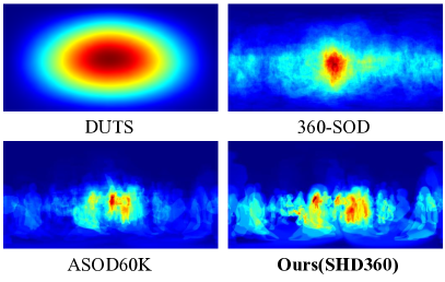
Dataset Bias. As shown in Figure 7, 360° datasets tend to show a equator bias, rather than only center bias existed in most of the 2D SOD datasets (e.g., DUTS [45]). Besides, our SHD360 shows relatively weaker center bias compared to other 360° datasets. The phenomenon is due to the photographers’ tendency of framing the salient targets parallel to the 360° cameras. Modeling such a bias may help improve performance and aid epistemic uncertainty estimation for explainable deep learning.

Figure 7: Ground truth distribution of different datasets, including DUTS [45], 360-SOD [28], ASOD60K [62] and our SHD360.

Evaluation Methods. To the best of our knowledge, so far there is no exclusive metric for the quantitative assessment of 360°-SOD. In addition, the only structure-focused SOD metric, S-measure [11], may not well adapted to the evaluation in ER images (Figure 5). The ER image captures a FoV of 360°$\times$180° thus owning large image area as background scenes, while relatively small object regions randomly distributed near the equator. However, the S-measure is designed for the situation where one or a few obvious foreground objects with appropriate size distributed near the center of the given 2D image. As a result, our $S_{\alpha}^{360}$ ((Eq. 2)) is proved to be more sensitive to the evaluation on 360° images (Figure 6). The $S_{\alpha}^{360}$ is able to give high score when the prediction is close to the ground truth, vice versa. The high sensitivity of our $S_{\alpha}^{360}$ is benefited from the cube map-based region similarity computation, which inspires future works toward fair comparison of object segmentation methods applied in 360° images and videos.

Appendix A General Metrics

In this work, we evaluate all 11 benchmark models with four widely used salient object detection (SOD) metrics and our proposed 360° geometry-adapted S-measure ($S_{\alpha}^{360}$), with respect to the ground-truth binary map and predicted saliency map. The F-measure ($F_{\beta}$) [1] and mean absolute error (MAE) [37] focus on the local (per-pixel) match between ground truth and prediction, while S-measure ($S_{\alpha}$) [11] and $S_{\alpha}^{360}$ pay attention to the object structure similarities (please refer to the manuscript for details). Besides, E-measure ($E_{\phi}$) [12] considers both the local and global information.

$\bullet$ MAE computes the mean absolute error between the ground truth $G\in\{0,1\}$ and a normalized predicted saliency map $P\in[0,1]$, i.e.,

$$MAE=\frac{1}{W\times{H}}\sum_{i=1}^{W}\sum_{j=1}^{H}\mid G(i,j)-P(i,j)\mid,$$ (3)

where $H$ and $W$ denote height and width, respectively.

$\bullet$ F-measure gives a single value ($F_{\beta}$) considering both the $Precision$ and $Recall$, which is defined as:

$$F_{\beta}=\frac{(1+\beta^{2})Precision\times Recall}{\beta^{2}Precision+Recall},$$ (4)

with

$$Precision=\frac{\left|P\cap G\right|}{\left|P\right|};Recall=\frac{\left|P\cap G\right|}{\left|G\right|},$$ (5)

where $P$ denotes a binary mask converted from a predicted saliency map and $G$ is the ground truth. Multiple $P$ are computed by assigning different thresholds $\tau,\tau\in[0,255]$ on the predicted saliency map. Note that the $\beta^{\text{2}}$ is set to 0.3 according to [1].

$\bullet$ E-measure is a cognitive vision-inspired metric to evaluate both the local and global similarities between two binary maps. Specifically, it is defined as:

$$E_{\phi}=\frac{1}{W\times H}\sum_{x=1}^{W}\sum_{y=1}^{H}\phi\left(P(x,y),G(x,y)\right),$$ (6)

where $\phi$ represents the enhanced alignment matrix [12].

Appendix B Experiments

In this section. we provide extensive results of our benchmark studies. Figure 9 shows attributes-specific F-/E-measure curves regarding all 11 baselines. Table 3 presents attributes-dependent quantitative result, which highlights relative good performance of baselines such as F3Net [21], LDF [50], CSF [15], PA-KRN [53], RCRNet [58] and PCSA [17]. Besides, we also provide sequence-based quantitative results in Table 4. Finally, we provide visual examples (Figure 11, 12 and 13) of qualitative results of all baselines upon our SHD360. Please also refer to ‘Demo-Outdoor-Tennis.mp4’ for complete visual results of a sequence example, i.e., OutDoor-Tennis.

	Metrics	SOD								VSOD		360° SOD
		CPD	SCRN	F3Net	MINet	LDF	CSF	GateNet	PA-KRN	RCRNet	PCSA	FANet
		[51]	[52]	[21]	[36]	[50]	[15]	[67]	[53]	[58]	[17]	[19]
MP	$F_{\beta}~{}\uparrow$	0.568	0.601	0.662	0.659	0.696	0.761	0.672	0.735	0.712	0.706	0.610
	$S_{\alpha}~{}\uparrow$	0.695	0.713	0.773	0.741	0.768	0.835	0.775	0.797	0.823	0.779	0.757
	$S_{\alpha}^{360}~{}\uparrow$	0.719	0.648	0.799	0.715	0.666	0.780	0.711	0.815	0.792	0.788	0.642
	$E_{\phi}~{}\uparrow$	0.710	0.714	0.889	0.830	0.869	0.896	0.814	0.874	0.882	0.826	0.679
	$\mathcal{M}~{}\downarrow$	0.031	0.029	0.024	0.026	0.025	0.017	0.023	0.024	0.022	0.026	0.032
OC	$F_{\beta}~{}\uparrow$	0.546	0.608	0.628	0.624	0.706	0.758	0.642	0.709	0.683	0.679	0.593
	$S_{\alpha}~{}\uparrow$	0.691	0.718	0.754	0.719	0.767	0.829	0.755	0.794	0.804	0.760	0.748
	$S_{\alpha}^{360}~{}\uparrow$	0.708	0.632	0.779	0.677	0.646	0.771	0.677	0.820	0.755	0.768	0.622
	$E_{\phi}~{}\uparrow$	0.716	0.741	0.861	0.818	0.878	0.902	0.796	0.876	0.881	0.828	0.684
	$\mathcal{M}~{}\downarrow$	0.024	0.022	0.018	0.020	0.017	0.012	0.019	0.018	0.017	0.020	0.025
DV	$F_{\beta}~{}\uparrow$	0.555	0.577	0.628	0.640	0.696	0.742	0.648	0.702	0.680	0.677	0.599
	$S_{\alpha}~{}\uparrow$	0.714	0.714	0.775	0.751	0.782	0.835	0.778	0.798	0.821	0.775	0.763
	$S_{\alpha}^{360}~{}\uparrow$	0.729	0.634	0.797	0.715	0.660	0.772	0.690	0.820	0.778	0.786	0.626
	$E_{\phi}~{}\uparrow$	0.745	0.706	0.879	0.848	0.893	0.903	0.816	0.882	0.889	0.828	0.689
	$\mathcal{M}~{}\downarrow$	0.015	0.015	0.013	0.013	0.012	0.009	0.013	0.012	0.011	0.012	0.017
MB	$F_{\beta}~{}\uparrow$	0.573	0.606	0.690	0.660	0.723	0.770	0.671	0.717	0.702	0.676	0.600
	$S_{\alpha}~{}\uparrow$	0.707	0.719	0.793	0.747	0.781	0.846	0.773	0.790	0.812	0.756	0.753
	$S_{\alpha}^{360}~{}\uparrow$	0.714	0.624	0.818	0.720	0.679	0.776	0.673	0.829	0.768	0.782	0.624
	$E_{\phi}~{}\uparrow$	0.729	0.716	0.882	0.843	0.883	0.909	0.813	0.861	0.887	0.794	0.682
	$\mathcal{M}~{}\downarrow$	0.025	0.024	0.016	0.020	0.018	0.012	0.019	0.020	0.017	0.021	0.027
OV	$F_{\beta}~{}\uparrow$	0.562	0.579	0.668	0.672	0.741	0.781	0.680	0.681	0.697	0.625	0.577
	$S_{\alpha}~{}\uparrow$	0.702	0.710	0.792	0.755	0.806	0.865	0.791	0.760	0.816	0.720	0.734
	$S_{\alpha}^{360}~{}\uparrow$	0.698	0.628	0.791	0.701	0.687	0.803	0.696	0.801	0.766	0.749	0.623
	$E_{\phi}~{}\uparrow$	0.722	0.682	0.892	0.869	0.911	0.931	0.840	0.846	0.896	0.757	0.664
	$\mathcal{M}~{}\downarrow$	0.029	0.028	0.020	0.023	0.020	0.013	0.022	0.025	0.021	0.027	0.032
GD	$F_{\beta}~{}\uparrow$	0.585	0.596	0.711	0.655	0.693	0.765	0.672	0.715	0.711	0.674	0.579
	$S_{\alpha}~{}\uparrow$	0.696	0.703	0.786	0.735	0.754	0.824	0.765	0.762	0.801	0.749	0.736
	$S_{\alpha}^{360}~{}\uparrow$	0.701	0.620	0.810	0.721	0.666	0.765	0.675	0.798	0.757	0.770	0.619
	$E_{\phi}~{}\uparrow$	0.694	0.689	0.878	0.807	0.828	0.866	0.785	0.822	0.850	0.770	0.643
	$\mathcal{M}~{}\downarrow$	0.055	0.054	0.043	0.050	0.048	0.040	0.048	0.050	0.046	0.051	0.058

Table 3: Attributes-based performance comparison of 11 baselines over our SHD360. $S_{\alpha}$ = S-measure ($\alpha$=0.5 [11]), $S_{\alpha}^{360}$ = 360° geometry-adapted S-measure, $F_{\beta}$ = mean F-measure ($\beta^{2}$=0.3) [1], $E_{\phi}$ = mean E-measure [12], $\mathcal{M}$ = mean absolute error [37]. $\uparrow$/$\downarrow$ denotes a larger/smaller value is better. Three best results of each row are in red, blue and green, respectively.

\begin{overpic}[width=429.28616pt]{Imgs/fig_pass_reject.pdf} \end{overpic}

Figure 8: Passed and rejected examples of annotation quality control process.

\begin{overpic}[width=429.28616pt]{Imgs/fig_curves_attr.pdf} \end{overpic}

Figure 9: Attributes-specific F-measure ($F_{\beta}$) and E-measure ($E_{\phi}$) curves of all 11 baselines upon our SHD360.

Super-class/	Metrics	SOD								VSOD		360° SOD
Sub-class		CPD [51]	SCRN [52]	F3Net [21]	MINet [36]	LDF [50]	CSF [15]	GateNet [67]	PA-KRN [53]	RCRNet [58]	PCSA [17]	FANet [19]
O./Japanese	$S_{\alpha}~{}\uparrow$	0.706	0.766	0.847	0.775	0.834	0.924	0.823	0.625	0.744	0.535	0.654
	max $E_{\phi}~{}\uparrow$	0.952	0.982	0.981	0.973	0.967	0.989	0.983	0.799	0.973	0.624	0.987
	mean $E_{\phi}~{}\uparrow$	0.637	0.664	0.947	0.934	0.904	0.951	0.865	0.685	0.880	0.464	0.559
	$\mathcal{M}~{}\downarrow$	0.047	0.044	0.019	0.033	0.025	0.017	0.030	0.043	0.039	0.056	0.054
I./SingingDancing	$S_{\alpha}~{}\uparrow$	0.594	0.620	0.671	0.562	0.601	0.700	0.601	0.842	0.725	0.644	0.712
	max $E_{\phi}~{}\uparrow$	0.967	0.982	0.981	0.724	0.683	0.983	0.983	0.968	0.986	0.909	0.991
	mean $E_{\phi}~{}\uparrow$	0.511	0.550	0.807	0.432	0.493	0.776	0.503	0.950	0.822	0.620	0.623
	$\mathcal{M}~{}\downarrow$	0.015	0.015	0.014	0.015	0.014	0.012	0.015	0.010	0.013	0.013	0.016
O./Walking	$S_{\alpha}~{}\uparrow$	0.923	0.757	0.959	0.952	0.812	0.968	0.886	0.759	0.899	0.891	0.816
	max $E_{\phi}~{}\uparrow$	0.995	0.989	0.994	0.994	0.970	0.996	0.992	0.869	0.993	0.985	0.995
	mean $E_{\phi}~{}\uparrow$	0.939	0.674	0.985	0.976	0.859	0.980	0.854	0.742	0.916	0.894	0.706
	$\mathcal{M}~{}\downarrow$	0.011	0.026	0.006	0.008	0.019	0.006	0.018	0.025	0.014	0.016	0.027
I./Melodrama	$S_{\alpha}~{}\uparrow$	0.744	0.774	0.823	0.793	0.764	0.861	0.858	0.773	0.830	0.792	0.747
	max $E_{\phi}~{}\uparrow$	0.896	0.951	0.900	0.889	0.860	0.958	0.966	0.852	0.943	0.863	0.947
	mean $E_{\phi}~{}\uparrow$	0.678	0.729	0.825	0.781	0.734	0.856	0.857	0.751	0.816	0.755	0.644
	$\mathcal{M}~{}\downarrow$	0.113	0.102	0.083	0.096	0.105	0.071	0.071	0.103	0.082	0.098	0.122
I./Studio	$S_{\alpha}~{}\uparrow$	0.690	0.675	0.839	0.783	0.808	0.832	0.797	0.814	0.868	0.888	0.760
	max $E_{\phi}~{}\uparrow$	0.977	0.983	0.984	0.986	0.988	0.980	0.988	0.984	0.988	0.991	0.993
	mean $E_{\phi}~{}\uparrow$	0.764	0.655	0.969	0.892	0.947	0.907	0.871	0.925	0.934	0.925	0.667
	$\mathcal{M}~{}\downarrow$	0.018	0.017	0.012	0.013	0.013	0.012	0.014	0.011	0.012	0.009	0.018
O./RacingCar	$S_{\alpha}~{}\uparrow$	0.381	0.387	0.508	0.372	0.393	0.430	0.401	0.399	0.415	0.369	0.377
	max $E_{\phi}~{}\uparrow$	0.457	0.798	0.555	0.336	0.371	0.510	0.640	0.382	0.545	0.313	0.533
	mean $E_{\phi}~{}\uparrow$	0.281	0.297	0.441	0.281	0.304	0.346	0.311	0.330	0.349	0.274	0.278
	$\mathcal{M}~{}\downarrow$	0.265	0.262	0.236	0.267	0.259	0.249	0.258	0.257	0.258	0.269	0.269
I./Violins	$S_{\alpha}~{}\uparrow$	0.741	0.724	0.826	0.854	0.825	0.890	0.881	0.751	0.899	0.755	0.781
	max $E_{\phi}~{}\uparrow$	0.978	0.982	0.980	0.980	0.982	0.987	0.985	0.976	0.988	0.972	0.989
	mean $E_{\phi}~{}\uparrow$	0.761	0.659	0.960	0.951	0.927	0.946	0.907	0.846	0.936	0.792	0.662
	$\mathcal{M}~{}\downarrow$	0.027	0.028	0.023	0.020	0.022	0.017	0.019	0.023	0.016	0.025	0.027
O./Football	$S_{\alpha}~{}\uparrow$	0.680	0.652	0.763	0.720	0.809	0.807	0.757	0.825	0.763	0.593	0.687
	max $E_{\phi}~{}\uparrow$	0.890	0.926	0.945	0.859	0.943	0.946	0.918	0.938	0.929	0.798	0.936
	mean $E_{\phi}~{}\uparrow$	0.700	0.542	0.828	0.830	0.897	0.866	0.818	0.905	0.826	0.515	0.626
	$\mathcal{M}~{}\downarrow$	0.004	0.003	0.004	0.003	0.003	0.003	0.004	0.002	0.004	0.005	0.006
I./Director	$S_{\alpha}~{}\uparrow$	0.732	0.782	0.825	0.779	0.799	0.889	0.852	0.814	0.863	0.840	0.823
	max $E_{\phi}~{}\uparrow$	0.970	0.972	0.973	0.969	0.973	0.987	0.977	0.970	0.977	0.975	0.991
	mean $E_{\phi}~{}\uparrow$	0.799	0.826	0.956	0.945	0.920	0.935	0.898	0.885	0.940	0.944	0.755
	$\mathcal{M}~{}\downarrow$	0.038	0.036	0.033	0.036	0.030	0.019	0.029	0.024	0.027	0.029	0.032
I./ChineseAd	$S_{\alpha}~{}\uparrow$	0.676	0.701	0.670	0.655	0.801	0.822	0.732	0.658	0.743	0.670	0.702
	max $E_{\phi}~{}\uparrow$	0.977	0.972	0.951	0.922	0.980	0.988	0.969	0.949	0.967	0.942	0.979
	mean $E_{\phi}~{}\uparrow$	0.811	0.722	0.641	0.774	0.954	0.948	0.773	0.773	0.887	0.838	0.679
	$\mathcal{M}~{}\downarrow$	0.010	0.004	0.014	0.005	0.003	0.003	0.005	0.012	0.006	0.006	0.009
I./Spanish	$S_{\alpha}~{}\uparrow$	0.773	0.808	0.884	0.827	0.844	0.868	0.830	0.842	0.862	0.812	0.740
	max $E_{\phi}~{}\uparrow$	0.929	0.963	0.969	0.968	0.969	0.974	0.964	0.956	0.964	0.928	0.963
	mean $E_{\phi}~{}\uparrow$	0.781	0.887	0.961	0.948	0.931	0.947	0.891	0.912	0.935	0.863	0.654
	$\mathcal{M}~{}\downarrow$	0.030	0.029	0.017	0.023	0.021	0.020	0.026	0.020	0.022	0.026	0.038
I./PianoSaxophone	$S_{\alpha}~{}\uparrow$	0.729	0.712	0.775	0.779	0.854	0.879	0.812	0.836	0.896	0.861	0.788
	max $E_{\phi}~{}\uparrow$	0.980	0.984	0.983	0.985	0.990	0.992	0.988	0.957	0.990	0.989	0.990
	mean $E_{\phi}~{}\uparrow$	0.732	0.663	0.951	0.888	0.956	0.932	0.858	0.942	0.936	0.914	0.703
	$\mathcal{M}~{}\downarrow$	0.013	0.014	0.015	0.011	0.010	0.008	0.012	0.012	0.009	0.009	0.016
I./BadmintonConvo	$S_{\alpha}~{}\uparrow$	0.572	0.600	0.765	0.648	0.693	0.909	0.694	0.648	0.771	0.620	0.610
	max $E_{\phi}~{}\uparrow$	0.775	0.937	0.928	0.875	0.913	0.977	0.949	0.751	0.941	0.718	0.965
	mean $E_{\phi}~{}\uparrow$	0.562	0.590	0.866	0.712	0.776	0.941	0.734	0.669	0.839	0.622	0.566
	$\mathcal{M}~{}\downarrow$	0.105	0.102	0.065	0.087	0.078	0.033	0.081	0.090	0.065	0.098	0.103
O./Beach	$S_{\alpha}~{}\uparrow$	0.615	0.656	0.607	0.688	0.693	0.636	0.648	0.668	0.632	0.668	0.593
	max $E_{\phi}~{}\uparrow$	0.858	0.906	0.866	0.907	0.832	0.925	0.932	0.822	0.928	0.929	0.940
	mean $E_{\phi}~{}\uparrow$	0.687	0.689	0.572	0.791	0.808	0.693	0.769	0.612	0.644	0.779	0.677
	$\mathcal{M}~{}\downarrow$	0.002	0.002	0.003	0.001	0.001	0.002	0.002	0.003	0.003	0.002	0.005
I./Brothers	$S_{\alpha}~{}\uparrow$	0.697	0.733	0.793	0.733	0.766	0.839	0.771	0.812	0.823	0.820	0.792
	max $E_{\phi}~{}\uparrow$	0.946	0.952	0.961	0.955	0.964	0.975	0.970	0.954	0.966	0.961	0.975
	mean $E_{\phi}~{}\uparrow$	0.732	0.761	0.945	0.875	0.904	0.929	0.846	0.932	0.909	0.922	0.708
	$\mathcal{M}~{}\downarrow$	0.019	0.017	0.015	0.015	0.015	0.012	0.017	0.012	0.015	0.013	0.020
I./Blues	$S_{\alpha}~{}\uparrow$	0.864	0.841	0.840	0.851	0.860	0.887	0.889	0.819	0.857	0.865	0.786
	max $E_{\phi}~{}\uparrow$	0.989	0.989	0.985	0.989	0.992	0.990	0.993	0.984	0.994	0.984	0.993
	mean $E_{\phi}~{}\uparrow$	0.922	0.897	0.964	0.970	0.971	0.964	0.935	0.916	0.907	0.954	0.688
	$\mathcal{M}~{}\downarrow$	0.012	0.011	0.011	0.010	0.008	0.007	0.010	0.008	0.011	0.009	0.015
I./Questions	$S_{\alpha}~{}\uparrow$	0.640	0.713	0.705	0.655	0.721	0.808	0.699	0.858	0.808	0.738	0.768
	max $E_{\phi}~{}\uparrow$	0.987	0.990	0.986	0.988	0.990	0.993	0.990	0.994	0.992	0.988	0.995
	mean $E_{\phi}~{}\uparrow$	0.630	0.774	0.852	0.761	0.883	0.887	0.725	0.958	0.896	0.782	0.656
	$\mathcal{M}~{}\downarrow$	0.015	0.014	0.013	0.014	0.011	0.009	0.012	0.008	0.010	0.011	0.016
O./Tennis	$S_{\alpha}~{}\uparrow$	0.762	0.689	0.825	0.809	0.826	0.847	0.816	0.855	0.807	0.815	0.782
	max $E_{\phi}~{}\uparrow$	0.967	0.967	0.985	0.976	0.979	0.984	0.983	0.980	0.979	0.978	0.988
	mean $E_{\phi}~{}\uparrow$	0.791	0.644	0.938	0.918	0.955	0.917	0.867	0.959	0.908	0.867	0.696
	$\mathcal{M}~{}\downarrow$	0.014	0.013	0.009	0.009	0.009	0.009	0.010	0.009	0.010	0.010	0.017
O./Sonwfield	$S_{\alpha}~{}\uparrow$	0.883	0.882	0.944	0.937	0.917	0.949	0.917	0.920	0.943	0.960	0.862
	max $E_{\phi}~{}\uparrow$	0.981	0.989	0.994	0.989	0.988	0.993	0.989	0.977	0.993	0.994	0.994
	mean $E_{\phi}~{}\uparrow$	0.900	0.906	0.987	0.974	0.973	0.969	0.937	0.932	0.974	0.980	0.744
	$\mathcal{M}~{}\downarrow$	0.023	0.020	0.008	0.013	0.014	0.011	0.017	0.017	0.011	0.009	0.032
I./PianoMono	$S_{\alpha}~{}\uparrow$	0.751	0.732	0.875	0.760	0.841	0.892	0.853	0.816	0.868	0.785	0.842
	max $E_{\phi}~{}\uparrow$	0.975	0.978	0.981	0.966	0.977	0.985	0.981	0.963	0.980	0.965	0.990
	mean $E_{\phi}~{}\uparrow$	0.776	0.749	0.967	0.923	0.938	0.965	0.923	0.944	0.932	0.836	0.752
	$\mathcal{M}~{}\downarrow$	0.034	0.034	0.021	0.037	0.025	0.020	0.026	0.036	0.026	0.028	0.031

Table 4: Sequence-specific performance comparison of 8/2/1 state-of-the-art SOD/VSOD/360° SOD methods. I. = indoor. O. = outdoor.

Sequence		General				360°		No.
		Multiple Persons	Occlusions	Distant View	Motion Blur	Out-of-View	Geometric Distortion
Indoor	French		✔		✔	✔	✔	4
	WaitingRoom	✔	✔	✔	✔			4
	Cooking	✔	✔	✔	✔		✔	5
	Guitar	✔		✔			✔	3
	Warehouse			✔	✔		✔	3
	Bass	✔	✔	✔			✔	4
	Passageway		✔	✔	✔	✔	✔	5
	RuralDriving						✔	1
	MICOSinging		✔				✔	2
	ScenePlay	✔					✔	2
	UrbanDriving						✔	1
	Clarinet	✔	✔				✔	3
	Interview		✔	✔				2
	Telephone				✔		✔	2
	Breakfast		✔	✔	✔		✔	4
	PianoSaxophone	✔	✔	✔		✔	✔	5
	Chorus	✔	✔	✔			✔	4
	Studio	✔		✔	✔		✔	4
	BadmintonConvo	✔	✔		✔	✔	✔	5
	Director	✔	✔	✔	✔		✔	5
	ChineseAd		✔	✔	✔	✔		4
	Blues	✔	✔	✔			✔	4
	Brothers	✔	✔	✔	✔	✔	✔	6
	Violins	✔		✔		✔	✔	4
	Spanish		✔		✔	✔	✔	4
	Questions	✔	✔	✔	✔		✔	5
	PianoMono				✔		✔	2
	Melodrama	✔					✔	2
	SingingDancing	✔	✔	✔	✔		✔	5
Outdoor	Bicycling		✔	✔	✔	✔	✔	5
	Japanese				✔	✔	✔	3
	Surfing		✔					1
	Lawn			✔	✔		✔	3
	AudiAd	✔	✔	✔	✔			4
	Walking			✔	✔		✔	3
	Bridge		✔	✔	✔			3
	RacingCar						✔	1
	Football			✔	✔	✔		3
	Snowfield				✔		✔	2
	Beach	✔	✔	✔	✔			4
	Tennis	✔	✔	✔	✔	✔	✔	6
No.		20	25	26	26	12	33	142

Table 5: Per-sequence attribute statistics.

\begin{overpic}[width=429.28616pt]{Imgs/fig_annotation_sum.pdf} \end{overpic}

Figure 10: Sample frames from SHD360, with instance-level ground truth overlaid.

\begin{overpic}[width=429.28616pt]{Imgs/fig_visual_te0.pdf} \end{overpic}

Figure 11: Visual results of all baselines upon SHD360-test0. Img = image. GT = ground truth.

\begin{overpic}[width=429.28616pt]{Imgs/fig_visual_te1.pdf} \end{overpic}

Figure 12: Visual results of all baselines upon SHD360-test1. Img = image. GT = ground truth.

\begin{overpic}[width=429.28616pt]{Imgs/fig_visual_te2.pdf} \end{overpic}

Figure 13: Visual results of all baselines upon SHD360-test2. Img = image. GT = ground truth.

References

- [1] Radhakrishna Achanta, Sheila Hemami, Francisco Estrada, and Sabine Süsstrunk. Frequency-tuned salient region detection. In IEEE CVPR, pages 1597–1604, 2009.
- [2] Ali Borji, Ming-Ming Cheng, Qibin Hou, Huaizu Jiang, and Jia Li. Salient object detection: A survey. Computational visual media, 5(2):117–150, 2019.
- [3] Markus Braun, Sebastian Krebs, Fabian Flohr, and Dariu M Gavrila. The eurocity persons dataset: A novel benchmark for object detection. arXiv preprint arXiv:1805.07193, 2018.
- [4] Hsien-Tzu Cheng, Chun-Hung Chao, Jin-Dong Dong, Hao-Kai Wen, Tyng-Luh Liu, and Min Sun. Cube padding for weakly-supervised saliency prediction in 360 videos. In IEEE CVPR, pages 1420–1429, 2018.
- [5] Shih-Han Chou, Cheng Sun, Wen-Yen Chang, Wan-Ting Hsu, Min Sun, and Jianlong Fu. 360-indoor: Towards learning real-world objects in 360deg indoor equirectangular images. In IEEE WACV, March 2020.
- [6] Xavier Corbillon, Francesca De Simone, and Gwendal Simon. 360-degree video head movement dataset. In MMSys, pages 199–204. ACM, 2017.
- [7] Navneet Dalal and Bill Triggs. Histograms of oriented gradients for human detection. In IEEE CVPR, volume 1, pages 886–893, 2005.
- [8] Jia Deng, Wei Dong, Richard Socher, Li-Jia Li, Kai Li, and Li Fei-Fei. Imagenet: A large-scale hierarchical image database. In IEEE CVPR, pages 248–255, 2009.
- [9] Piotr Dollar, Christian Wojek, Bernt Schiele, and Pietro Perona. Pedestrian detection: An evaluation of the state of the art. IEEE TPAMI, 34(4):743–761, 2012.
- [10] Deng-Ping Fan, Ming-Ming Cheng, Jiang-Jiang Liu, Shang-Hua Gao, Qibin Hou, and Ali Borji. Salient objects in clutter: Bringing salient object detection to the foreground. In ECCV, pages 186–202, 2018.
- [11] Deng-Ping Fan, Ming-Ming Cheng, Yun Liu, Tao Li, and Ali Borji. Structure-measure: A new way to evaluate foreground maps. In IEEE ICCV, pages 4548–4557, 2017.
- [12] Deng-Ping Fan, Cheng Gong, Yang Cao, Bo Ren, Ming-Ming Cheng, and Ali Borji. Enhanced-alignment measure for binary foreground map evaluation. IJCAI, pages 698–704, 2018.
- [13] Deng-Ping Fan, Zheng Lin, Zhao Zhang, Menglong Zhu, and Ming-Ming Cheng. Rethinking rgb-d salient object detection: Models, data sets, and large-scale benchmarks. IEEE TNNLS, 2020.
- [14] Deng-Ping Fan, Wenguan Wang, Ming-Ming Cheng, and Jianbing Shen. Shifting more attention to video salient object detection. In IEEE CVPR, 2019.
- [15] Shang-Hua Gao, Yong-Qiang Tan, Ming-Ming Cheng, Chengze Lu, Yunpeng Chen, and Shuicheng Yan. Highly efficient salient object detection with 100k parameters. In ECCV, 2020.
- [16] Ke Gong, Xiaodan Liang, Dongyu Zhang, Xiaohui Shen, and Liang Lin. Look into person: Self-supervised structure-sensitive learning and a new benchmark for human parsing. In IEEE CVPR, pages 932–940, 2017.
- [17] Yuchao Gu, Lijuan Wang, Ziqin Wang, Yun Liu, Ming-Ming Cheng, and Shao-Ping Lu. Pyramid constrained self-attention network for fast video salient object detection. In AAAI, 2020.
- [18] Hou-Ning Hu, Yen-Chen Lin, Ming-Yu Liu, Hsien-Tzu Cheng, Yung-Ju Chang, and Min Sun. Deep 360 pilot: Learning a deep agent for piloting through 360 sports videos. In IEEE CVPR, pages 1396–1405, 2017.
- [19] Mengke Huang, Zhi Liu, Gongyang Li, Xiaofei Zhou, and Olivier Le Meur. Fanet: Features adaptation network for 360° omnidirectional salient object detection. IEEE Signal Processing Letters, 27:1819–1823, 2020.
- [20] Haroon Idrees, Imran Saleemi, Cody Seibert, and Mubarak Shah. Multi-source multi-scale counting in extremely dense crowd images. In IEEE CVPR, pages 2547–2554, 2013.
- [21] Qingming Huang Jun Wei, Shuhui Wang. F3net: Fusion, feedback and focus for salient object detection. In AAAI, 2020.
- [22] Chen Li, Mai Xu, Xinzhe Du, and Zulin Wang. Bridge the gap between vqa and human behavior on omnidirectional video: A large-scale dataset and a deep learning model. In ACM MM, pages 932–940, 2018.
- [23] Fuxin Li, Taeyoung Kim, Ahmad Humayun, David Tsai, and James M Rehg. Video segmentation by tracking many figure-ground segments. In IEEE ICCV, pages 2192–2199, 2013.
- [24] Guanbin Li, Yuan Xie, Liang Lin, and Yizhou Yu. Instance-level salient object segmentation. In IEEE CVPR, pages 2386–2395, 2017.
- [25] Guanbin Li, Yuan Xie, Tianhao Wei, Keze Wang, and Liang Lin. Flow guided recurrent neural encoder for video salient object detection. In IEEE CVPR, pages 3243–3252, 2018.
- [26] Guanbin Li and Yizhou Yu. Visual saliency based on multiscale deep features. In IEEE CVPR, pages 5455–5463, 2015.
- [27] Haofeng Li, Guanqi Chen, Guanbin Li, and Yu Yizhou. Motion guided attention for video salient object detection. In IEEE ICCV, 2019.
- [28] Jia Li, Jinming Su, Changqun Xia, and Yonghong Tian. Distortion-adaptive salient object detection in 360∘ omnidirectional images. IEEE JSTSP, 14(1):38–48, 2019.
- [29] J. Li, C. Xia, and X. Chen. A benchmark dataset and saliency-guided stacked autoencoders for video-based salient object detection. IEEE TIP, 27(1):349–364, 2018.
- [30] Yin Li, Xiaodi Hou, Christof Koch, James M Rehg, and Alan L Yuille. The secrets of salient object segmentation. In IEEE CVPR, pages 280–287, 2014.
- [31] Jiang-Jiang Liu, Qibin Hou, Ming-Ming Cheng, Jiashi Feng, and Jianmin Jiang. A simple pooling-based design for real-time salient object detection. In IEEE CVPR, 2019.
- [32] Si Liu, Zitian Wang, Yulu Gao, Lejian Ren, Yue Liao, Guanghui Ren, Bo Li, and Shuicheng Yan. Human-centric relation segmentation: Dataset and solution. IEEE TPAMI, 2021.
- [33] Xiankai Lu, Wenguan Wang, Chao Ma, Jianbing Shen, Ling Shao, and Fatih Porikli. See more, know more: Unsupervised video object segmentation with co-attention siamese networks. In IEEE CVPR, 2019.
- [34] Guangxiao Ma, Shuai Li, Chenglizhao Chen, Aimin Hao, and Hong Qin. Stage-wise salient object detection in 360° omnidirectional image via object-level semantical saliency ranking. IEEE TVCG, 26(12):3535–3545, 2020.
- [35] Peter Ochs, Jitendra Malik, and Thomas Brox. Segmentation of moving objects by long term video analysis. IEEE TPAMI, 36(6):1187–1200, 2014.
- [36] Youwei Pang, Xiaoqi Zhao, Lihe Zhang, and Huchuan Lu. Multi-scale interactive network for salient object detection. In IEEE CVPR, June 2020.
- [37] Federico Perazzi, Philipp Krähenbühl, Yael Pritch, and Alexander Hornung. Saliency filters: Contrast based filtering for salient region detection. In IEEE CVPR, pages 733–740, 2012.
- [38] Federico Perazzi, Jordi Pont-Tuset, Brian McWilliams, Luc Van Gool, Markus Gross, and Alexander Sorkine-Hornung. A benchmark dataset and evaluation methodology for video object segmentation. In IEEE CVPR, pages 724–732, 2016.
- [39] Xuebin Qin, Zichen Zhang, Chenyang Huang, Chao Gao, Masood Dehghan, and Martin Jagersand. Basnet: Boundary-aware salient object detection. In IEEE CVPR, June 2019.
- [40] Yashas Rai, Jesús Gutiérrez, and Patrick Le Callet. A dataset of head and eye movements for 360 degree images. In MMSys, pages 205–210. ACM, 2017.
- [41] Sucheng Ren, Chu Han, Xin Yang, Guoqiang Han, and Shengfeng He. Tenet: Triple excitation network for video salient object detection. In ECCV, pages 212–228. Springer, 2020.
- [42] Vincent Sitzmann, Ana Serrano, Amy Pavel, Maneesh Agrawala, Diego Gutierrez, Belen Masia, and Gordon Wetzstein. Saliency in vr: How do people explore virtual environments? IEEE TVCG, 24(4):1633–1642, 2018.
- [43] Alexander Toshev and Christian Szegedy. Deeppose: Human pose estimation via deep neural networks. In IEEE CVPR, pages 1653–1660, 2014.
- [44] Rahul Rama Varior, Mrinal Haloi, and Gang Wang. Gated siamese convolutional neural network architecture for human re-identification. In ECCV, pages 791–808. Springer, 2016.
- [45] Lijun Wang, Huchuan Lu, Yifan Wang, Mengyang Feng, Dong Wang, Baocai Yin, and Xiang Ruan. Learning to detect salient objects with image-level supervision. In IEEE CVPR, pages 136–145, 2017.
- [46] Wenguan Wang, Qiuxia Lai, Huazhu Fu, Jianbing Shen, Haibin Ling, and Ruigang Yang. Salient object detection in the deep learning era: An in-depth survey. IEEE TPAMI, 2021.
- [47] Wenguan Wang, Jianbing Shen, and Ling Shao. Consistent video saliency using local gradient flow optimization and global refinement. IEEE TIP, 24(11):4185–4196, 2015.
- [48] Xueyang Wang, Xiya Zhang, Yinheng Zhu, Yuchen Guo, Xiaoyun Yuan, Liuyu Xiang, Zerun Wang, Guiguang Ding, David Brady, Qionghai Dai, et al. Panda: A gigapixel-level human-centric video dataset. In IEEE CVPR, pages 3268–3278, 2020.
- [49] Zhou Wang, Alan C Bovik, Hamid R Sheikh, and Eero P Simoncelli. Image quality assessment: from error visibility to structural similarity. IEEE TIP, 13(4):600–612, 2004.
- [50] Jun Wei, Shuhui Wang, Zhe Wu, Chi Su, Qingming Huang, and Qi Tian. Label decoupling framework for salient object detection. In IEEE CVPR, June 2020.
- [51] Zhe Wu, Li Su, and Qingming Huang. Cascaded partial decoder for fast and accurate salient object detection. In IEEE CVPR, June 2019.
- [52] Zhe Wu, Li Su, and Qingming Huang. Stacked cross refinement network for edge-aware salient object detection. In IEEE ICCV, October 2019.
- [53] Binwei Xu, Haoran Liang, Ronghua Liang, and Peng Chen. Locate globally, segment locally: A progressive architecture with knowledge review network for salient object detection. In AAAI, volume 35, pages 3004–3012, 2021.
- [54] Mai Xu, Chen Li, Yufan Liu, Xin Deng, and Jiaxin Lu. A subjective visual quality assessment method of panoramic videos. In ICME, pages 517–522. IEEE, 2017.
- [55] Mai Xu, Chen Li, Shanyi Zhang, and Patrick Le Callet. State-of-the-art in 360 video/image processing: Perception, assessment and compression. IEEE JSTSP, 14(1):5–26, 2020.
- [56] Mai Xu, Yuhang Song, Jianyi Wang, MingLang Qiao, Liangyu Huo, and Zulin Wang. Predicting head movement in panoramic video: A deep reinforcement learning approach. IEEE TPAMI, 2018.
- [57] Yanyu Xu, Yanbing Dong, Junru Wu, Zhengzhong Sun, Zhiru Shi, Jingyi Yu, and Shenghua Gao. Gaze prediction in dynamic 360 immersive videos. In IEEE CVPR, pages 5333–5342, 2018.
- [58] Pengxiang Yan, Guanbin Li, Yuan Xie, Zhen Li, Chuan Wang, Tianshui Chen, and Liang Lin. Semi-supervised video salient object detection using pseudo-labels. In IEEE ICCV, pages 7284–7293, 2019.
- [59] Qiong Yan, Li Xu, Jianping Shi, and Jiaya Jia. Hierarchical saliency detection. In IEEE CVPR, pages 1155–1162, 2013.
- [60] Chuan Yang, Lihe Zhang, Huchuan Lu, Xiang Ruan, and Ming-Hsuan Yang. Saliency detection via graph-based manifold ranking. In IEEE CVPR, pages 3166–3173, 2013.
- [61] Wenyan Yang, Yanlin Qian, Joni-Kristian Kamarainen, Francesco Cricri, and Lixin Fan. Object detection in equirectangular panorama. In IEEE ICPR, pages 2190–2195, 2018.
- [62] Yi Zhang, Fang-Yi Chao, Ge-Peng Ji, Deng-Ping Fan, Lu Zhang, and Ling Shao. Asod60k: Audio-induced salient object detection in panoramic videos. arXiv e-prints, pages arXiv–2107, 2021.
- [63] Yi Zhang, Lu Zhang, Wassim Hamidouche, and Olivier Deforges. A fixation-based 360∘ benchmark dataset for salient object detection. In IEEE ICIP, 2020.
- [64] Ziheng Zhang, Yanyu Xu, Jingyi Yu, and Shenghua Gao. Saliency detection in 360 videos. In ECCV, pages 488–503, 2018.
- [65] Jia-Xing Zhao, Jiang-Jiang Liu, Deng-Ping Fan, Yang Cao, Jufeng Yang, and Ming-Ming Cheng. Egnet:edge guidance network for salient object detection. In IEEE ICCV, Oct 2019.
- [66] Pengyu Zhao, Ansheng You, Yuanxing Zhang, Jiaying Liu, Kaigui Bian, and Yunhai Tong. Spherical criteria for fast and accurate 360° object detection. In AAAI, pages 12959–12966, 2020.
- [67] Xiaoqi Zhao, Youwei Pang, Lihe Zhang, Huchuan Lu, and Lei Zhang. Suppress and balance: A simple gated network for salient object detection. In ECCV, 2020.
- [68] Huajun Zhou, Xiaohua Xie, Jian-Huang Lai, Zixuan Chen, and Lingxiao Yang. Interactive two-stream decoder for accurate and fast saliency detection. In IEEE CVPR, June 2020.
- [69] Chen Zuyao, Xu Qianqian, Cong Runmin, and Huang Qingming. Global context-aware progressive aggregation network for salient object detection. In AAAI, 2020.