An Elementary Solution To Lambert’s Problem

Abstract

A fundamental problem in spacecraft mission design is to find a free-flight path from one place to another with a given transfer time. This problem for paths in a central force field is known as Lambert’s problem. Although this is an old problem, we take a new approach. Given two points in the plane, we produce the conic parameters $(p,e,\omega)$ for all conic paths between these points. For a given central force gravitational parameter, the travel time between the launch and destination points is computed along with the initial and final velocities for each transfer conic. For a given travel time, we calculate the parameters for a transfer conic having that travel time.

1 Introduction

Lagrange showed in 1778 that the time required to traverse an elliptic arc between specified endpoints for Kepler’s problem depends only on the semi-major axis of the ellipse, the distance between the two points, and the sum of their distances from the focus of the ellipse. A wide range of methods for solving Lambert’s problem have subsequently been proposed over the years with various areas of applicability for different problems. These methods often focus on the use of various parameters such as F & G series (Bate et al., 1971), universal variables (Vallado, 2013), and semimajor axis (Prussing and Conway, 2013) just to mention a few. Other standard solutions to Lambert’s problem can be found in Pollard (1966), Battin (1999), and Gooding (1990). A more complete description of various Lambert problem solutions may be found in Russell (2019). Many of these approaches focus on the proper selection of variables to use in combination with the time-of-flight to optimize subsequent convergence on a desired time-of-flight using various iteration methods.

The textbook solution to Lambert’s problem typically derives the transfer time using Kepler’s equation and the eccentric anomalies of the endpoints. To calculate travel times between points on a transfer conic arc we use conservation of angular momentum and numerical integration. This avoids using Kepler’s equation and eccentric anomalies. In our approach, we first focus on determining the set of all elliptical orbit solutions that connect two points. We use a geometric approach based on standard orbital elements that eliminates the need for using various intermediate parameters that may not always have an obvious physical meaning. In particular, the conic parameters $p$ and $e$ (the scale parameter and eccentricity) form a triangle in the parameter plane for the elliptical transfer orbit case, which is the basis of our approach.

In the final section, the results presented here are used to construct a sequence of conic arcs between a sequence of patch points as an application. The method is general and can be extended to construct conic arcs between patch points in three dimensions. The method can be used as a preliminary mission design tool producing a sequence of conic arcs between a sequence of patch points which could include maneuvers or flybys.

2 A Geometry Problem

For two points with polar coordinates $(R,\alpha)$ and $(R\gamma,\alpha+\phi)$ with $\gamma>1$, the first step of the problem is to find the parameters of all conic arcs between them. The equation of a general conic has the form

$$r(\theta)=\frac{p}{1+e\cos(\theta-\omega)}$$ (1)

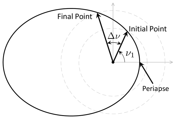
where $\nu=\theta-\omega$ is the true anomaly and $r$ is the radius. A general conic is defined by its parameters $(p,e,\omega)$. The scale parameter $p$ and the elliptic parameter, or eccentricity, $e$ are non-negative. A standard conic as we define it here has the argument of periapse $\omega=0$. Coordinate rotation by $\omega$ takes the conic with parameters $(p,e,0)$ to the conic with parameters $(p,e,\omega)$. Suppose a standard conic with parameters $(p,e,0)$ contains the points with polar coordinates $(1,\nu_{1})$ and $(\gamma,\nu_{1}+\Delta\nu)$ as shown in Figure 1. Here, the initial true anomaly $\nu_{1}$ is also referred to as the inside angle, and the change in the true anomaly $\Delta\nu$ is called the transfer angle.

Figure 1: Schematic showing the standard conic with $\nu_{1}$ and $\nu_{2}=\nu_{1}+\Delta\nu$.

Then the rotated and rescaled conic with parameters $(Rp,e,\alpha-\nu_{1})$ contains the points $(R,\alpha)$ and $(R\gamma,\alpha+\Delta\nu)$. We will rotate and rescale to produce transfer conics from standard conics.

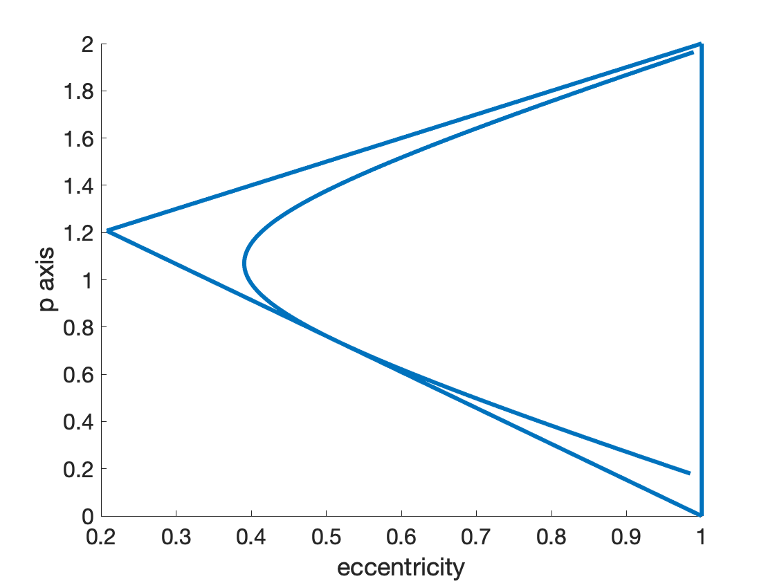
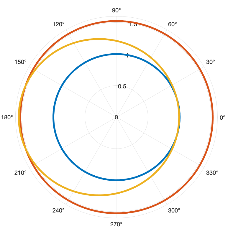
Given circles of radius $1$ and radius $\gamma>1$ centered at the origin of a plane, we first find all standard ellipses that intersect both circles. The minimum and maximum radii of an ellipse with parameters $(p,e,0)$ are equal to $p/(1+e)$ and $p/(1-e)$, respectively. Necessary and sufficient conditions for intersections with the circles are $p/(1+e)\leq 1\leq\gamma\leq p/(1+e)$. The set of points in the $(p,e)$ plane which satisfy these conditions forms a triangle $T(\gamma)$ as shown in Figure 2 for $\gamma=1.524$. The value 1.524 was used because this is the roughly the distance of the orbit of Mars from the Sun in astronomical units. The triangle is bounded by the lines $e=1,p=1+e$, and $p=\gamma(1-e)$. For conics with $e\geq 1$ the condition for intersection is $p/(1+e)\leq 1$.

Figure 2: Allowed elliptic parameters

A standard conic with parameters $(p,e,0)$ generates two equations for its intersections with the two circles:

$$\frac{p}{1+e\cos(\nu_{1})}=1$$ (2)

$$\frac{p}{1+e\cos(\nu_{2})}=\gamma$$ (3)

The cosines $(c_{1},c_{2})$ of the angles $(\nu_{1},\nu_{2})$ are found by solving the equations

$$p=1+ec_{1}$$ (4)

$$\frac{p}{\gamma}=1+ec_{2}$$ (5)

The solution defines a map

$$f:T(\gamma)\to[-1,1]\times[-1,1]$$ (6)

$$f(p,e)=(c_{1},c_{2})=((p-1)/e,(p-\gamma)/e\gamma)$$ (7)

The inverse of this map has the formula

$$f^{-1}(c_{1},c_{2})=(1+c_{1}(\gamma-1)/(c_{1}-\gamma c_{2}),(\gamma-1)/(c_{1}-\gamma c_{2}))$$ (8)

The set $T^{*}(\gamma)=f(T(\gamma))$ is also a triangle contained in the square $[-1,1]\times[-1,1]$. The top boundary of $T^{*}(\gamma)$ is the image of the boundary of $T(\gamma)$ with $e=1$. By using the formula for $f^{-1}$ one shows that this boundary is the line segment

$$c_{2}=\gamma^{-1}(c_{1}+1)-1,\,-1\leq c_{1}\leq 1.$$ (9)

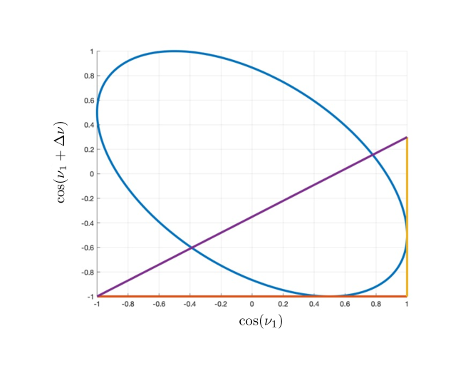
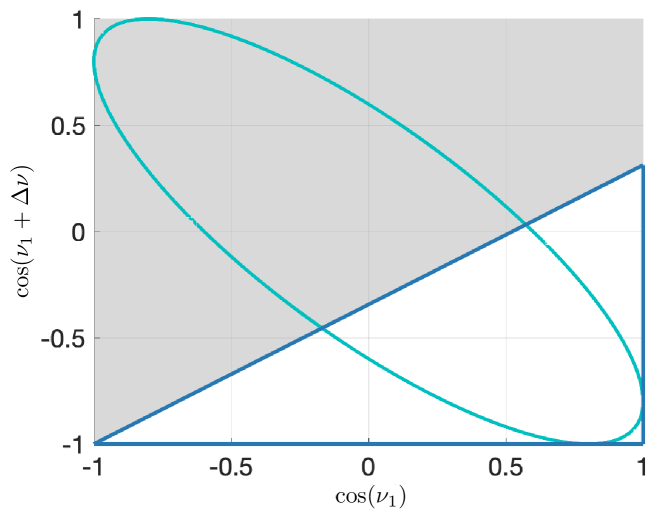
The triangle $T^{*}(1.524)$ is shown in Figure 3. The cosine oval $Oval(\Delta\nu)$ shown in the plot is the parameterized curve $Oval(x)=(\cos(x),\cos(x+\Delta\nu))$ for $0\leq x\leq 2\pi$. The intersection of the oval with the triangle will be used to solve for the parameters of all standard ellipses that intersect the circles at points with coordinates of the form $(1,\nu_{1})$, and $(\gamma,\nu_{1}+\Delta\nu)$.

Figure 3: The set $Oval(\Delta\nu)$ and $T^{*}(\gamma)$ for $\gamma=1.524$ and $\Delta\nu=\pi/3$

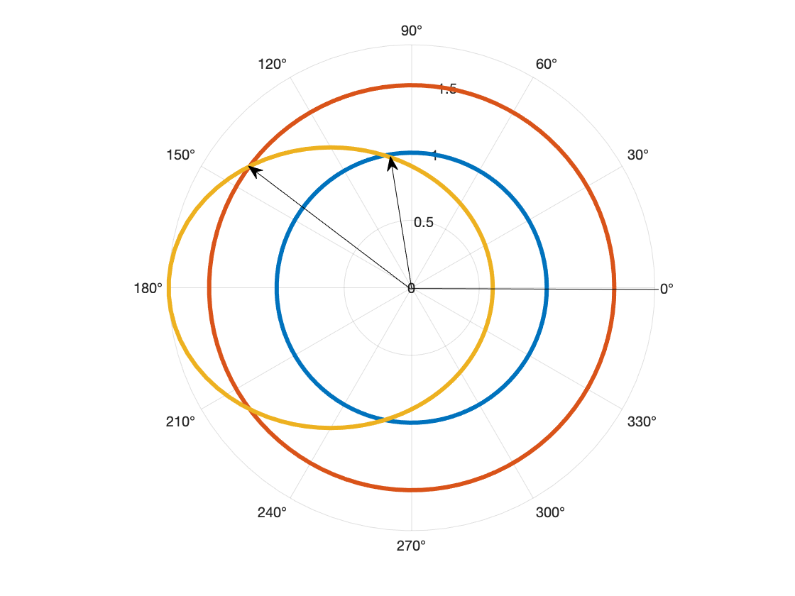
An example of a standard ellipse intersecting two circles is shown in Figure 4.

Figure 4: Circles of radius 1 and radius 1.5. Elliptic parameters $p=.9,e=.5,\omega=0$. Angles $\nu$ and $\Delta\nu$ are shown.

For a given transfer angle draw the oval and intersect this oval with the image $T^{*}(\gamma)$ of the map $f$. The intersection determines an interval of allowed inside angles $\nu_{1}(\Delta\nu,\gamma)\leq\nu\leq\nu_{2}(\Delta\nu,\gamma)$ . The intersection points of the cosine oval $Oval(\Delta\nu)$ with the upper boundary of the triangle $T^{*}(\gamma)$ are found by finding the solutions $\nu_{1}$ and $\nu_{2}$ of the equation

$$\cos(\nu_{2})=\gamma^{-1}(\cos(\nu_{1})+1)-1$$ (10)

where $\nu_{2}=\nu_{1}+\Delta\nu$. A typical intersection is shown in Figure 3 for $\Delta\nu=\pi/3$. The preimage of the intersection $Oval(\Delta\nu)\cap T^{*}(\gamma)$ of the cosine oval as viewed in the $p$-$e$ plane is shown in Figure 5. This shows the elliptic parameters of the transfer ellipses with transfer angle $\Delta\nu$.

Figure 5: The preimage of the set $T^{*}(\gamma)\cap Oval(\Delta\nu)$ viewed in the e-p plane.

To compute the set of allowed elliptic parameters $f^{-1}[T^{*}(\gamma)\cap Oval(\Delta\nu)]$ one uses the map

$$g:[\nu_{1}(\Delta\nu,\gamma),\nu_{2}(\Delta\nu,\gamma)]\to R^{2}$$ (11)

$$g(\nu_{1})=f^{-1}(\cos(\nu_{1}),\cos(\nu_{1}+\Delta\nu))$$ (12)

$$g(\nu_{1})=(p(\gamma,\Delta\nu,\nu_{1}),e(\gamma,\Delta\nu,\nu_{1}))$$ (13)

$$e(\gamma,\Delta\nu,\nu_{1})=[\gamma-1]/[\cos(\nu_{1})-\gamma\cos(\nu_{1}+\Delta\nu)]$$ (14)

$$p(\gamma,\Delta\nu,\nu_{1})=e(\gamma,\Delta\nu,\nu_{1})\cos(\nu_{1})+1$$ (15)

The function $g$ determines the set of allowed elliptic parameters of transfer ellipses as a function of the outer radius and the transfer and inner angles. The function$f^{-1}$ applied to the set $Oval(\Delta\nu)$ also determines the set of all conic transfer parameters. To create elliptic arcs joining the points $(R_{1},\alpha)$ and $(R_{2},\alpha+\Delta\nu)$, choose $\gamma=R_{2}/R_{1}$. Choose elliptic parameters$(p(\gamma,\Delta\nu,\nu_{1}),e(\gamma,\Delta\nu,\nu_{1}))$. These are the parameters of a standard ellipse that intersects the inner and outer circles with the transfer angle $\Delta\nu$ and inside angle $\nu_{1}$. Set $\omega=\alpha-\nu_{1}$. The angle is the argument of the periapse of a rotated standard ellipse. Then the transfer ellipse between the points $(R_{1},\alpha)$ and $(R_{2},\alpha+\Delta\nu)$ is the general conic

$$r(\theta)=R_{1}p(\gamma,\Delta\nu,\nu_{1})/[1+e(\gamma,\Delta\nu,\nu_{1})\cos(\theta-\omega)]$$ (16)

When the inside angle $\nu_{1}$ is unconstrained, the formula (16) produces parabolas and hyperbolas.

3 Travel Times

As a first step to determining the transfer orbit between two points for a specific time, the transfer orbits for all times may be computed. Consider travel times for a given gravitational parameter $\mu$, from an inner radius $R$ to an outer radius $\gamma R$ . The travel times depend on the values of $(\mu,R,\gamma,\Delta\nu,\nu_{1})$. Consider travel times for standard conics as a function of these variables. Use equations (14) and (15) to produce parameters $p(\gamma,\Delta\nu,\nu_{1})$, $e(\gamma,\Delta\nu,\nu_{1})$ for a standard conic with the chosen transfer and inner angles. Then compute travel times using the following algorithm.

Algorithm: travel times as a function of $(\mu,R,\gamma,\Delta\nu,\nu_{1})$.

1. Calculate $(e(\gamma,\Delta\nu,\nu_{1}),p(\gamma,\Delta\nu,\nu_{1}))=(e,p)$ using equations (14) and (15).

2. Set $P=Rp$ (rescale), $\sigma=\sqrt{\mu p}$ (angular momentum)

3. Integrate using the formula $r^{2}(\theta)d\theta=\sigma dt$

4. $T=\sigma^{-1}R^{2}p^{2}\int_{\nu_{1}}^{\nu_{1}+\Delta\nu}(1+ecos(\theta))^{-2}d\theta$ (travel time)

5. For fixed parameters $(\mu,R,\gamma,\Delta\nu)$ and for a given travel time $\tau$, solve the equation $T(\mu,R,\gamma,\Delta\nu,\nu_{1})=\tau$ for $\nu_{1}^{*}$ .

6. Calculate the parameters $(e(\gamma,\Delta\nu,\nu_{1}^{*}),p(\gamma,\Delta\nu,\nu_{1}^{*}))=(e^{*},p^{*})$ of the transfer ellipse.

The time to travel from $(R,\,\alpha)$ to $(\gamma R,\alpha+\Delta\nu)$ on the transfer ellipse

$$r(\theta)=Rp(\gamma,\Delta\nu,\nu_{1})/[1+e(\gamma,\Delta\nu,\nu_{1})cos(\theta-\omega)]$$ (17)

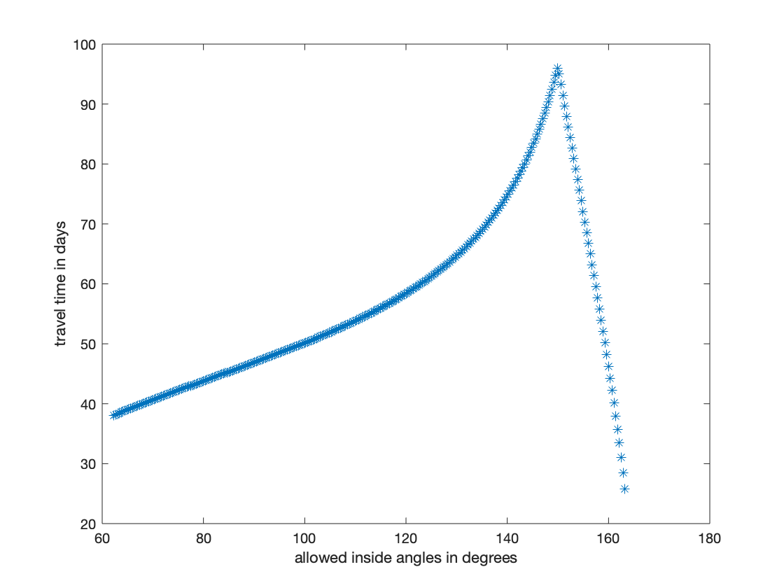
with $\omega=\alpha-\nu_{1}$ is the same as the time to travel on the corresponding standard ellipse with $\omega=0$ . Thus the travel time does not depend on $\omega$. Steps 5 and 6 solve Lambert’s problem. Travel times for $\mu=1.327*10^{11}\,km^{3}/s^{2},\,\gamma=1.524,\,\Delta\nu_{1}=\pi/6$ are displayed in Figure 6 as a function of the admissible inside angles.

Figure 6: Travel times for allowed inside angles $\nu_{1}$ for $\gamma=1.524$ and $\Delta\nu=\pi/6$

4 Specific Travel Time Solution

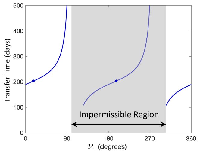
Once the possible transfer orbits have been computed as a function of the inside angle $\nu_{1}$, the possible transfer orbits with a specific transfer time may be computed. A standard method for finding the zero of a function may then be used, and some sample results were computed next using Matlab’s fzero function. As an example, we consider the Mars 2020 transfer trajectory which launched on July 30, 2020 and arrived on February 18, 2021. The angle between launch and landing points is about 143.2 degrees, and the travel time is about 203 days. The allowable range of inside angles $(\nu_{1},\nu_{2})$ may first be computed by finding the intersections of the oval with the triangle as shown in Figure 7. The permissible values of $\cos(\nu_{1})$ and $\cos(\nu_{2})$ are given by the non-shaded region.

Figure 7: The set $Oval(\Delta\nu)$ and $T^{*}(\gamma)$ for $\gamma=1.524$ and $\Delta\nu=143.2$ degrees.

By plotting the transfer time as a function of $\nu_{1}$, the different possible solutions between the two desired points may now be clearly seen as shown in Figure 8. By using different initial guesses for $\nu_{1}$, the algorithm can converge on possible different zeros along the curve.

Figure 8: Travel time as a function of $\nu_{1}$ for the Mars 2020 trajectory.

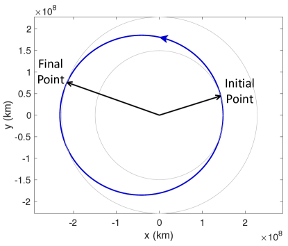
By limiting the search space to the allowable $\nu_{1}$ values and using the algorithm, the solution converged to $(\nu_{1},e,p)$ = (0.302347076950009, 0.21911558915832, 1.20917656075465). The geometry of this ellipse is shown in Figure 9. While these results were computed for the dimensionless orbits in the plane, the actual transfer orbits may be computed in three dimensions by simply scaling and rotating the resulting orbits in combination with using states from the ephemeris.

(a) Dimensionless ellipse

(b) Dimensional transfer

Figure 9: A transfer ellipse with elliptic parameters $(e,p)$ = (0.21911558915832, 1.20917656075465) is plotted along with circles of radius 1 and radius 1.524. The inside angle $\nu_{1}$ was approximately 0.302347076950009.

5 Conclusion

A new elementary approach to Lambert’s problem based on computing all conic transfer orbits between two points is derived as a function of the polar coordinate of the points and the initial true anomaly. This method was successfully used to compute these conic transfers across a range of possible transfer times for the direct case using elliptic orbits. By implementing a straightforward zero finding method, it is possible to compute specific orbits with desired transfer times using a standard conic. This approach solves Lambert’s problem once subsequent standard rotations are performed to orient the orbit correctly in three-dimensional space. The presented approach also allows the computation of various constraints on the possible astrodynamic parameters for each transfer, which reduces the search space and speeds up the computation of the desired solution.

6 Acknowledgements

Part of the research presented in this paper has been carried out at the Jet Propulsion Laboratory, California Institute of Technology, under a contract with the National Aeronautics and Space Administration. The authors would like to thank James Meiss and David Sterling for valuable comments and suggestions.

Appendix A Appendix: Velocity Changes at Patch Points

In this section the formulas for transfer conics and transfer times are applied to design patched conic orbits. To transfer from one arc to the next on a patched conic path, one must know the angle between the tangent lines to the arcs at the patch point. For a general conic with equation

$$r(\theta)=\frac{p}{1+e\cos(\theta-\omega)}$$ (18)

The angle $\Phi$ of a unit tangent vector to the conic at a point $(r(\theta),\theta)$ on the conic is required for this calculation. To find this angle one can calculate using complex variables. For this calculation the notation for eccentricity conflicts with exponential notation. Just for this calculation the symbol for eccentricity will be $\epsilon$.

$$q(\theta)=r(\theta)e^{i\theta},\dot{q}(\theta)=\dot{r}(\theta)e^{i\theta}+r(\theta)ie^{i\theta}=s(\theta)e^{i\Phi}$$ (19)

$$s(\theta)=\sqrt{\dot{r}(\theta)^{2}+(r(\theta)^{2}}$$ (20)

$$\dot{r}(\theta)+r(\theta)i=s(\theta)e^{i(\Phi-\theta)}$$ (21)

$$sin(\Delta\nu-\theta)=r(\theta)/s(\theta)$$ (22)

$$\Phi=\theta+asin(r(\theta)/s(\theta))$$ (23)

$$\dot{r}(\theta)=(\epsilon/p)r^{2}(\theta)sin(\theta-\omega)$$ (24)

$$\dot{r}(\theta)/r(\theta)=[1+\epsilon cos(\theta-\omega)]^{-1}\epsilon sin(\theta-\omega)$$ (25)

$$r(\theta)/s(\theta)=1/\sqrt{\epsilon^{2}sin^{2}(\theta-\omega)/{[1+\epsilon cos(\theta-\omega)]}^{2}+1}$$ (26)

Now replace $\epsilon$ by $e$ as the symbol for eccentricity. The result is

$$\Phi=\theta+asin(1/\sqrt{\epsilon^{2}sin^{2}(\theta-\omega)/r^{2}(\theta)+1}\,)$$ (27)

The energy of the orbit in terms of the elliptic parameters $(p,\,e,\,\omega)$ is $E=\mu(e^{2}-1)/2p$. For an elliptic orbit of the Kepler problem $\ddot{q}=-\mu r^{{}_{3}}\,\,with\,r=|q|$ The Cartesian velocity $v(r,\theta)=\dot{q}$ is the velocity at the point $(r,\theta)$ on the conic and the speed is

$$s(r,\theta)=|\dot{q}|=\sqrt{2(E+\mu r^{-1})}=\sqrt{2\mu}\sqrt{[(e^{2}-1)/p]+r^{-1}}$$ (28)

The velocity in polar coordinates is $(s(r,\mu,e,p),\Phi(r,\theta,e,p,\omega))$. To transfer from an incoming elliptic orbit to an outgoing elliptic orbit at a common patch point $(r,\theta)$ the velocity change needed is the difference between the outgoing and incoming velocities at this point. These velocities are determined for polar coordinates by the above formulas.

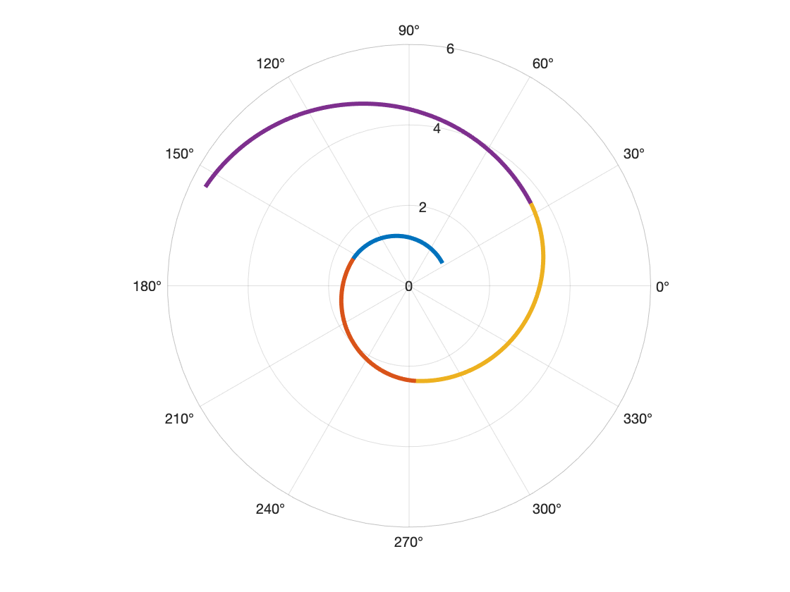
To patch elliptic arcs in an outward spiral one can go back to geometry and choose conic arcs between circles of radii $1,\,\gamma,\gamma^{2},...$ with a fixed transfer angle $\Delta\nu$ between patch points and choose allowed elliptic parameters $(1\,,e_{0},\omega_{0})$. Then choose an initial scale parameter and generate a sequence of elliptic parameters $p_{1}=\gamma p_{0},\,e_{1}=e_{0},\omega_{1}=\omega_{0}+\Delta\nu,\,...$ Elliptic arcs, travel times, and velocity changes can now be computed from this data. A plot for the choice $\gamma=1.524,\,\Delta\nu=2\pi/3,\,p_{0}=1.202,\,e_{0}=.2385$ is shown in Figure 10.

Figure 10: Four conic arcs with $\gamma=1.524,\,\Delta\nu=2\pi/3\,\,p_{0}=1.202,\,e_{0}=.2385$

References

- Bate et al. (1971) Bate RR, Mueller DD, White JE (1971) Fundamentals of Astrodynamics. Dover Publications, Inc., New York
- Battin (1999) Battin RH (1999) An Introduction to the Mathematics and Methods of Astrodynamics, Revised edn. AIAA Education Series
- Gooding (1990) Gooding RH (1990) A procedure for the solution of lambert’s orbital boundary-value problem. Celestial Mechanics and Dynamical Astronomy 48(2):145–165
- Pollard (1966) Pollard H (1966) Mathematical Introduction to Celestial Mechanics. Prentice-Hall Inc., Englewood Cliffs, New Jersey
- Prussing and Conway (2013) Prussing JE, Conway BA (2013) Orbital Mechanics, 2nd edn. Oxford University Press, New York
- Russell (2019) Russell RP (2019) On the solution to every Lambert problem. Celestial Mechanics and Dynamical Astronomy pp 131–150
- Vallado (2013) Vallado DA (2013) Fundamentals of Astrodynamics and Applications, 4th edn. Space Technology Library, Microcosm Press