Deep Descriptive Clustering

Abstract

Recent work on explainable clustering allows describing clusters when the features are interpretable. However, much modern machine learning focuses on complex data such as images, text, and graphs where deep learning is used but the raw features of data are not interpretable. This paper explores a novel setting for performing clustering on complex data while simultaneously generating explanations using interpretable tags. We propose deep descriptive clustering that performs sub-symbolic representation learning on complex data while generating explanations based on symbolic data. We form good clusters by maximizing the mutual information between empirical distribution on the inputs and the induced clustering labels for clustering objectives. We generate explanations by solving an integer linear programming that generates concise and orthogonal descriptions for each cluster. Finally, we allow the explanation to inform better clustering by proposing a novel pairwise loss with self-generated constraints to maximize the clustering and explanation module’s consistency. Experimental results on public data demonstrate that our model outperforms competitive baselines in clustering performance while offering high-quality cluster-level explanations.

1 Introduction

As machine learning is applied to more complex data and situations, the need to understand a model’s decisions becomes more paramount. The area of explainable AI (XAI) Adadi and Berrada (2018) is motivated to enhance the interpretability of complex machine learning models, especially deep learning. Arguably XAI is more needed and more challenging in unsupervised learning such as clustering as the explanations are usually at the model level rather than the instance level. For example, supervised learning explanations mainly focus on why an instance is classified to a specific class Ribeiro et al. (2016); however, with clustering we need to explain the semantics of each discovered cluster.

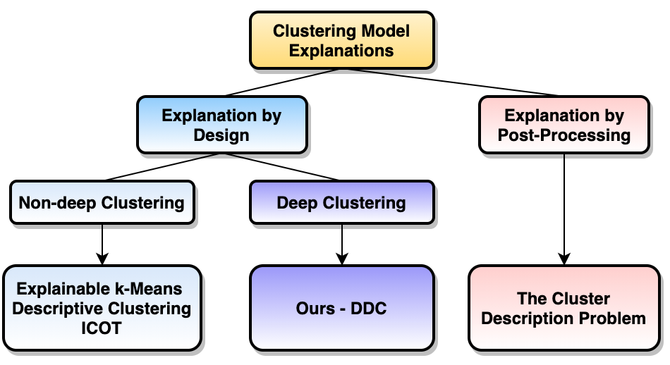
Figure 1: Taxonomy of works on clustering explanations.

Existing work on explainable clustering (see Figure 1) typically takes one of two directions: i) explanation by design algorithms Bertsimas et al. (2020); Moshkovitz et al. (2020) that use interpretable features to create both a clustering and an explanation (left branch of Figure 1). ii) explanation by post-processing Davidson et al. (2018); Sambaturu et al. (2020) which take an existing clustering and generate an explanation using another additional set of features (tags) not given to the clustering algorithm (right branch of Figure 1). Each direction has its limitations: the first type of work is not suitable for complex data such as images and graphs as the underlying features are uninterpretable to a human. Post-processing methods are algorithm-agnostic, but they did not fully use the information from additional features to guide the clustering process hence may generate poor explanations as the clustering may be difficult to explain. Instead, our proposed method will learn a good clustering that is also interpretable while post-processing approaches only find the best explanation possible for a given clustering.

Explaining deep clustering results using the underlying complex features is a challenging but alternative direction. Instead, we explore the situation that a partial set of instance-level semantic tags are known from which we generate a cluster-level description along with complex features to cluster on. This setting is not uncommon and was previously studied Dao et al. (2018); Davidson et al. (2018). Example settings include Twitter graphs where the user-user graph is clustered and explained using hashtags and personal images where the tags are descriptors of events in the image.

To address the challenges of simultaneously clustering and explaining efficiently with incomplete semantic features, we propose a novel deep descriptive clustering framework (DDC) that incorporates both deep clustering and cluster-level explanation. The whole framework is trained iteratively to maximize the consistency between the clustering and its explanation. To be specific, we formulate the cluster-level description problem as an Integer Linear Programming (ILP) which is solved for concise and orthogonal descriptions for each cluster. Inspired by the success of the discriminative clustering model Krause et al. (2010) which has fewer assumptions of the data, our main clustering objective maximizes the mutual information between empirical distribution on the inputs and the induced clustering labels. Finally, we propose a pairwise loss with self-generated constraints to penalize the inconsistency between the clustering feature space and discovered descriptive tag space to improve the clustering quality. The major contributions of this paper are listed as follows:

• We propose a novel framework to learn clustering and cluster-level explanations simultaneously. The proposed architecture supports learning from the sub-symbolic level (which clustering is performed on) and symbolic level (which explanations are created from).

• We formulate the class-level explanation problem as an ILP to solve concise and orthogonal explanations. A pairwise loss function is proposed with self-generated constraints to bridge the clustering and explanation.

• Empirical results on public data demonstrate that our model consistently achieves better clustering results and high-quality explanations compared to recent baselines.

• We explore the novel direction of graphical ontology explanations for clustering when the number of clusters is large and a lengthy explanation list is problematic.

The rest of this paper is organized as follows. In section 2, we overview related works. We then introduce our learning objectives and optimization algorithms in section 3. Experimental results and analysis are reported in section 4. Finally, section 5 concludes this paper with future research directions.

2 Related Work

Explainable clustering models.

Many previous works Liu et al. (2005); Fraiman et al. (2013); Ghattas et al. (2017); Bertsimas et al. (2020) have explored the explainable-by-design algorithms which consider the simultaneous construction of decision trees and cluster discovery for explainable clustering. Typical work such as Moshkovitz et al. (2020) considered traditional clustering algorithms like k-medians/means. However, one major limitation of these methods is that they require the features used for clustering to be interpretable which may not be the case for complex data such as graphs and images. Another line of research Davidson et al. (2018); Sambaturu et al. (2020) assumes one set of semantic tags for each instance are available to do post-processing explanation. Davidson et al. (2018) proposed a model-agnostic explanation method that explains any given clustering with tags but does not change the clustering. Perhaps the closest work to our own is Dao et al. (2018) but is limited to simple diameter-based clustering objectives and scales to just a few thousand instances whilst making strong assumptions such as having well-annotated tags for every instance. Our work differs from the above: we learn a deep clustering model and cluster explanation simultaneously with a partial set of semantic tags and scales for large data sets.

Multi-view clustering.

As our approach uses semantic tags for explanation this can be seen as another view of the data; hence we overview the recent works on multi-view clustering and discuss how our proposed work differentiates from it. The goal of multi-view clustering Bickel and Scheffer (2004); Xu et al. (2013); Shao et al. (2015); Tao et al. (2017); Wang et al. (2018); Hu and Chen (2018) is getting better clustering results via exploiting complementary and consensus information across multiple views rather than simply concatenating different views. Our descriptive clustering setting is different from multi-view clustering: Firstly, instead of just one goal which maximizes clustering performance, our work has another explanation objective to find meaningful descriptions of clusters. Secondly, most multi-view clustering is for similar views (i.e., all images) whereas our views are more diverse (e.g., continuous image features with categorical semantic tags) than general multi-view clustering settings.

Constrained clustering.

Unlike most multi-view clustering algorithms which leverages the knowledge from different views to maximize the clustering performance, constrained clustering assumes the users have access to partial pre-existing knowledge about the desired partition of the data. The constraints are usually expressed via pairwise constraints Wagstaff et al. (2001); Bilenko et al. (2004); Basu et al. (2008) such as together and apart which indicates whether two instances belong to the same cluster or different clusters. Recent works Fogel et al. (2019); Zhang et al. (2019) have also extended constrained clustering to deep learning models. Our work shares one common attribute with these works in using a constrained optimization objective for better clustering. However, in this work our constraints are dynamically self-generated in that they cannot be known a priori as generating those constraints require both the feature representation and the clustering explanations.

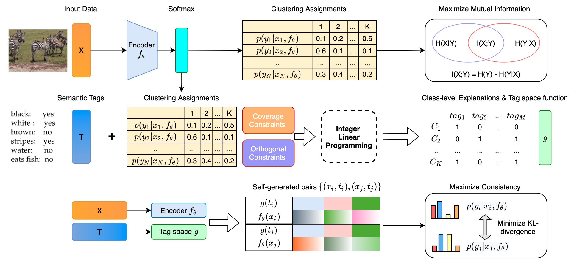
Figure 2: The framework of deep descriptive clustering (DDC). DDC consists of one clustering objective, one sub-symbolic explanation objective, and one self-generated objective to maximize the consistency between clustering and explanation modules.

3 Approach

3.1 Overall Framework

The framework of our proposed Deep Descriptive Clustering (DDC) is shown in Figure 2. It can be divided into three learning objectives: i) clustering objective which maximizes the mutual information between the empirical distribution on the inputs and the induced label distribution; ii) class-level explanation objective which finds the shortest and different explanations for each cluster and creates a tag space mask function $g$ to filter out uninformative tags; iii) an instance pairwise loss term with self-generated constraints to maximize the consistency between the clustering feature space and the descriptive tag space induced by mask function $g$.

3.2 Information Maximization for Clustering

Given unlabeled dataset of $N$ data points as $X=\{x_{1},...,x_{N}\}$ where $x_{i}=(x_{i1},...,x_{iD})\in{\mathbb{R}}^{D}$ are $D$ dimensional feature vectors, the goal of our proposed model is to predict the clustering assignments $y\in\{1,...,K\}$ given input $x$, encoding network $f_{\theta}$ and cluster size $K$. Inspired by RIM Krause et al. (2010) which learns a probabilistic clustering model $p(y|x,\mathcal{W})$ with parameters $\mathcal{W}$ to maximize the mutual information between $x$ and $y$, we represent the estimated mutual information Bridle et al. (1992) between $x$ and $y$ with network $f_{\theta}$ as the difference between marginal entropy $H(Y)$ and conditional entropy $H(Y{\mid}X)$. Our clustering objective maximizes the mutual information $I(X;Y)$ via minimizing loss $\mathcal{L}_{MI}$:

$$\begin{split}\mathcal{L}_{MI}&=-I(X;Y)=H(Y{\mid}X)-H(Y)\\ &=\frac{1}{N}\sum_{i=1}^{N}h(p(y_{i}|x_{i},f_{\theta}))-h(\frac{1}{N}\sum_{i=1}^{N}p(y_{i}|x_{i},f_{\theta}))\end{split}$$ (1)

where $h$ is the entropy function and $p(y_{i}|x_{i},f_{\theta})$ is calculated through $f_{\theta}$ and $K$-way softmax function. Intuitively minimizing conditional entropy $H(Y{\mid}X)$ will map similar $x$ to have similar clustering predictions $y$ and maximizing the entropy $H(Y)$ will incorporate the notion of class balance to avoid degenerate solution such as all the points map to one class.

3.3 The Cluster-level Explanation Objective

In addition to the unlabeled data $X$, to provide high-level explanations we assume a set of partial annotated tags $T=\{t_{1},...t_{N}\}$ where $t_{i}=(t_{i1},...,t_{iM})\in{\mathbb{R}}^{M}$ is a binary vector. In real world applications assuming each instance has a complete set of annotated tags is unlikely, thus we assume each instance’s tag can be missing with a specified probability $r$. With the predicted clustering assignments $Y$ we can partition both $X$ and $T$ into $K$ clusters.

We formulate the cluster-level description problem as an Integer Linear Programming (ILP) to learn short and orthogonal descriptors for each cluster. Specifically, we solve for the $K\times M$ binary allocation matrix $W$ where $W_{i,j}=1$ iff cluster $C_{i}$ is described by tag $j$. The main objective function is to find the most concise overall cluster description:

$$\operatorname*{arg\,min}_{W}\sum_{i,j}W_{ij}$$ (2)

Our first constraint set includes the explanation length requirement for each cluster explicitly and set coverage constraints implicitly. Given a fixed number of tags as explanations for discovered cluster $C_{i}$, a high coverage explanation indicates that most instances within cluster $C_{i}$ contain the selected tags. Now we define the fraction of cluster $i$ having tag $j$ as $Q_{ij}=\frac{1}{|C_{i}|}\sum_{t_{k}\in C_{i}}t_{kj}$. Note we use mean imputation for missing tags. Formally we expect at least $\alpha$ tags being selected to explain each cluster:

$$\sum_{j=1}^{M}W_{ij}Q_{ij}\geq\alpha\quad\forall i\in\{1,..K\}$$ (3)

Combining Eq (3) with our main objective in Eq (2), the constraint set in Eq (3) will naturally require the ILP solver to select tags that have higher coverage within each cluster.

Our next orthogonal constraint requires that the tags chosen to represent each cluster have minimum overlap which encourages informative explanations. Denote the hyper-parameter $\beta$ as the upper-bound of expected number of overlapping tags per cluster, the orthogonal constraint can be encoded as follow:

$$\sum_{i=1}^{K}W_{ij}Q_{ij}\leq\beta\quad\forall j\in\{1,..M\}$$ (4)

Lastly we have the regular constraints to make $W$ a valid binary matrix as $W_{ij}\in\{0,1\}$. There are $KM$ variables to solve and $K+M$ constraints for set coverage and orthogonal requirements. Our proposed ILP objective can be solved efficiently due to the cluster-level explanation design ($K\ll N$). Empirical results have shown that our ILP module’s running time only takes $1\%$ of the whole framework’s training time.

Now we define the tag space mapping function $g$ which is used in our next objective. Let the solution for our proposed cluster-level explanation problem be $W^{*}$. We define function $g$ for all the data as $g(t_{i})=t_{i}*G$ where $G\in{\mathbb{R}}^{M\times M}$ is a diagonal matrix such that $G_{jj}=1$ iff tag $j$ is used in explanation allocation matrix $W^{*}$. Note function $g$ can be treated as a mask function to filter out less informative semantic tags solved by our proposed cluster-level explanation objectives.

3.4 Self-generated Pairwise Loss Term

Our first proposed objective trains network $f_{\theta}$ for clustering; the second objective solves for explanations and a tag space function $g$. We propose a pairwise loss objective to reconcile inconsistencies between the two by finding instances that share similar informative descriptors but from different clusters, that is $g(t_{i})\approx g(t_{j})$ but $f_{\theta}(x_{i})\neq f_{\theta}(x_{j})$. To achieve this we introduce a pairwise loss objective to bridge the explanation and clustering module. This part is important because our goal is to use semantic tags to generate explanations and reshape the clustering features for better clustering. Previous works on constrained clustering Wagstaff et al. (2001); Basu et al. (2008) have shown that adding pairwise guidance such as together and apart constraints to clustering modules can largely improve clustering performance. However, these algorithms assume the pairwise guidance is given as ground-truth. In our setting we propose to add self-generated pairwise constraints with the assumption that instances which are close in tag space should be close in clustering feature space. Formally for each instance $x_{i}$ we search for top $l$ instances which minimize the objective $J$ for self-generated together constraints:

$$\begin{split}J_{i}=&\min_{j\in\{1,...,N\}}\gamma*|g(t_{i})-g(t_{j})|-|f_{\theta}(x_{i})-f_{\theta}(x_{j})|\end{split}$$ (5)

where $\gamma$ is the penalizing weight for tag space’s difference. Minimizing $J$ requires accessing the whole training set which is inefficient for mini-batch training. Instead we replace $N$ with batch size $N_{B}$ and solve an approximated version of Eq (5) in each mini-batch. We generate $l$ pairs of together constraints for each instance $x_{i}$ and then directly minimize the KL divergence between the clustering predictions $y_{i}$ and $y_{j}$:

$$\begin{split}\mathcal{L}_{P}=&\frac{1}{Nl}\sum_{i=1}^{N}\sum_{j=1}^{l}KL(p(y_{i}|x_{i},f_{\theta}),p(y_{j}|x_{j},f_{\theta}))\\ \end{split}$$ (6)

Eq (6) minimizes the inconsistency between the clustering feature space and the semantic tag space and reshapes the clustering feature space for better clustering and explanation.

Algorithm 1 Algorithm for Deep Descriptive Clustering

0:  Data $X=\{x_{1},...,x_{N}\}$, tags $T=\{t_{1},...,t_{N}\}$, number of clusters $K$, hyper-parameters $\alpha,\beta,\gamma,\lambda$.

0:  Clustering partitions $\{C_{1},...C_{K}\}$, well-trained $f_{\theta}$ and $g$, explanation allocation matrix $W^{*}$.

1:  Initialize network $f_{\theta}$ and tag space function $g$.

2:  Pre-train $f_{\theta}$ via back-propagating overall loss in Eq (7).

3:  repeat

4:     Construct cluster-level explanation problem as ILP defined in Eq (2,3,4). Initialize $\beta=0$, $W^{*}=\emptyset$.

5:     while ILP solution $W^{*}$ is not feasible do

6:        Increase hyper-parameter $\beta$ by the fixed step size $1$.

7:        Solve the ILP for $W^{*}$ and tag space function $g$.

8:     end while

9:     for each mini-batch do

10:        Generate pairwise constraints based on the objective $J$ in Eq (5) within each batch.

11:        Calculate the pairwise loss $\mathcal{L}_{P}$ via Eq (6) and the clustering loss $\mathcal{L}_{MI}$ via Eq (1).

12:        Update network parameters $f_{\theta}$ by minimizing overall loss $\mathcal{L}$ in Eq (7).

13:     end for

14:  until Network $f_{\theta}$ and explanation results converge

3.5 Overall Training Algorithm

Algorithm 1 presents our training algorithm for the deep descriptive clustering. Firstly we initialize the clustering network $f_{\theta}$ with random weights and initialize the weight matrix $G$ of function $g$ as identity matrix. Then we minimize the overall loss $\mathcal{L}$ by combining the clustering objective $\mathcal{L}_{MI}$ and pairwise loss term $\mathcal{L}_{P}$ with weight $\lambda$:

$$\begin{split}\mathcal{L}&=\frac{\lambda}{Nl}\sum_{i=1}^{N}\sum_{j=1}^{l}KL(p(y_{i}|x_{i},f_{\theta}),p(y_{j}|x_{j},f_{\theta}))+\\ &\frac{1}{N}\sum_{i=1}^{N}h(p(y_{i}|x_{i},f_{\theta}))-h(\frac{1}{N}\sum_{i=1}^{N}p(y_{i}|x_{i},f_{\theta}))\end{split}$$ (7)

Given the clustering predictions we construct the cluster-level explanation problem with binary variable $W$ and calculate $Q$ values for all the discovered clusters $\{C_{1},...C_{K}\}$. Note given the expected number of tags used for each cluster as $\alpha$, we run our ILP solver iteratively with linear search for the smallest feasible hyper-parameter $\beta$ to ensure tightest orthogonal constraints. Once the binary explanation allocation matrix $W^{*}$ is solved, we update the tag space function $g$ and regenerate the pairwise constraints via objective $J$ to maximize the consistency between clustering features and tag space. The whole model is trained repetitively until convergence.

C	Composition by animals	Description by tags	TC $\uparrow$	ITF $\uparrow$
C1	1 grizzly bear, 2 dalmatian, 1 horse, 2 blue whale	big, fast, strong, muscle, new world, smart	0.94	1.34
C2	5 antelope, 2 grizzly bear, 2 beaver, 5 dalmatian, 5 Persian cat, 5 horse, 6 German shepherd, 3 Siamese cat	furry, chew teeth, fast, quadrupedal, new world, ground	0.98	0.94
C3	69 beaver, 64 dalmatian, 42 Persian cat, 29 blue whale, 42 Siamese cat	tail, fast, new world, timid, smart, solitary	0.98	1.17
C4	100 killer whale, 69 blue whale, 1 Siamese cat	tail, fast, fish, smart	1.00	1.10
C5	95 antelope, 97 grizzly bear, 29 beaver, 29 dalmatian, 53 Persian cat, 94 horse, 94 German shepherd, 54 Siamese cat	furry, chew teeth, fast, quadrupedal, new world, ground	1.00	0.94

Table 1: Results generated by descriptive clustering Dao et al. (2018), we present the first Pareto point of their result such that the diameter of all the clusters are minimized. $\uparrow$ means the larger value the better.

C	Composition by animals	Description by tags	TC $\uparrow$	ITF $\uparrow$
C1	100 grizzly bear, 100 beaver	tough skin, bulbous, paws, quadrupedal, nocturnal, hibernate, smart, solitary	1.00	2.32
C2	100 Siamese cat, 100 Persian cat	white, gray, pads, chew teeth, claws, weak, inactive, old world	1.00	2.32
C3	100 antelope, 100 dalmatian	furry, big, long leg, active, new world, ground, timid, group	1.00	2.32
C4	100 killer whale, 100 blue whale	spots, hairless, flippers, strain teeth, fish, plankton, arctic, ocean	1.00	2.32
C5	100 horse, 100 German shepherd	black, brown, patches, smelly, walks, strong, agility, domestic	1.00	2.32

Table 2: Results generated by our proposed DDC. $\uparrow$ means the larger value the better.

4 Experiments

In this section, we conduct experiments to evaluate our approach empirically. Based on our experiments, we aim to answer the following questions:

• Can our proposed approach generate better explanations compared to existing methods? (see Sec 4.2) Can it generate more complex explanations such as ontologies (see Sec 4.3)?

• How does our proposed approach perform in terms of clustering quality? (see Sec 4.4)

• How does simultaneously clustering and explaining improve our model’s performance? (see Sec 4.5)

4.1 Experimental Setup

Data.

We evaluate the performance of our proposed model on two visual data sets with annotated semantic attributes. We first use Attribute Pascal and Yahoo (aPY) Farhadi et al. (2009), a small-scale coarse-grained dataset with $64$ semantic attributes and $5274$ instances. We have selected $15$ classes for our clustering task. Further, we have studied Animals with Attributes (AwA) Lampert et al. (2013), which is a medium-scale dataset in terms of the number of images. For AwA we use $85$ semantic attributes and $19832$ instances, we have set $40$ classes for clustering, the total number of animals.

Baselines and Evaluation Metrics.

In the experiments, deep descriptive clustering is compared with descriptive clustering Dao et al. (2018) in terms of the explanation quality. To evaluate the generated explanations quantitatively and qualitatively, we list all the composition and selected tags for each discovered cluster and report the Tag Coverage (TC) and Inverse Tag Frequency (ITF). For cluster $C_{i}$, let the descriptive tag set be $D_{i}$, the TC and ITF for $C_{i}$ are calculated as:

$$TC(C_{i})=\frac{1}{|D_{i}|}\sum_{d\in D_{i}}\frac{|\{(x,t)\in C_{i}:d\in t\}|}{|C_{i}|}$$ (8)

$$ITF(C_{i})=\frac{1}{|D_{i}|}\sum_{d\in D_{i}}\log\frac{K}{\sum_{j=1}^{K}|d\in D_{j}|}$$ (9)

The Tag Coverage for $C_{i}$ ranges from $[0,1]$ and the max value is achieved when each descriptive tag exists in all the instances within $C_{i}$. The Inverse Tag Frequency for $C_{i}$ ranges from $[0,\log K]$ and the max value is achieved when each descriptive tag is only used once. For both TC and ITF the larger the better. We have also generated a graphical ontology as high-level explanation on the clustering results when the number of clusters is large and a long explanation list is problematic. We evaluate its quality by comparing it to human knowledge.

Further, we evaluate the clustering performance with a range of tag annotated ratios $r$ as [$10\%,30\%,50\%$] and compare DCC’s results against vanilla k-means clustering and competitive incomplete multi-view clustering approaches such as MIC, IMG, and DAIMC Shao et al. (2015); Zhao et al. (2016); Hu and Chen (2018). For the clustering evaluation metric, we choose to use both Normalized Mutual Information (NMI) Strehl et al. (2000) and Clustering Accuracy (ACC) Xu et al. (2003) for comprehensive evaluation.

Implementations.

For a fair comparison with all the baseline approaches, we use pre-trained ResNet-101 He et al. (2016) features for all the clustering tasks and the encoder networks of deep descriptive clustering model are stacked by three fully connected layers with size of $[1200,1200,K]$ where $K$ is the desired number of clusters. We set the expected number of tags for each cluster as $8$ and hyper-parameters $l,\lambda,\gamma$ as $1,1,100$ respectively. The tag annotated ratio $r$ is set as $0.5$ by default to simulate a challenging setting. The activation function is ReLU, and the optimizer is Adam Kingma and Ba (2015) with default parameters.

4.2 Comparison with Descriptive Clustering

We duplicate the experimental setting in Dao et al. (2018) by down-sampling $10$ classes from AwA and cluster the data into $5$ clusters for a fair comparison. We list the explanation results in Table 1 and 2. Our model’s Tag Coverage values for all the clusters are $1$; this result shows that our model successfully maximizes the consistency between the discovered tag space and clustering feature space so that similar instances with similar tags are grouped. Moreover, the Inverse Tag Frequency values of our model are much higher than the competing method. This result indicates that our model selects informative tags for each cluster that differentiate from other discovered clusters. We also observe that our proposed model generates high-quality clusters where similar animals are correctly grouped together. Finally, we have found one attribute’s annotation error in the AwA data when examining our explanations for $C_{1}$; the beavers are annotated with attribute hibernate but the truth is the opposite. This finding suggests that the labeled attributes are noisy in the AwA data set.

		NMI			ACC
Datasets	Methods $r\%$	10	30	50	10	30	50
AwA	K-Means	$\text{71.67}\pm\text{0.63}$	$\text{73.72}\pm\text{0.66}$	$\text{74.23}\pm\text{0.69}$	$\text{66.21}\pm\text{0.57}$	$\text{67.98}\pm\text{0.60}$	$\text{68.24}\pm\text{0.54}$
	IMG	$\text{71.86}\pm\text{2.41}$	$\text{74.43}\pm\text{2.69}$	$\text{82.16}\pm\text{3.01}$	$\text{66.19}\pm\text{2.05}$	$\text{69.17}\pm\text{2.25}$	$\text{76.24}\pm\text{2.78}$
	MIC	$\text{72.40}\pm\text{1.68}$	$\text{76.85}\pm\text{1.71}$	$\text{83.43}\pm\text{1.89}$	$\text{67.26}\pm\text{1.45}$	$\text{70.52}\pm\text{1.58}$	$\text{77.68}\pm\text{1.84}$
	DAIMC	$\text{72.88}\pm\text{2.38}$	$\text{79.02}\pm\text{2.46}$	$\text{87.10}\pm\text{2.74}$	$\text{67.87}\pm\text{1.97}$	$\text{73.14}\pm\text{2.13}$	$\text{82.34}\pm\text{2.39}$
	Ours DCC	$\textbf{75.62}\pm\textbf{1.17}$	$\textbf{83.93}\pm\textbf{1.35}$	$\textbf{89.57}\pm\textbf{1.37}$	$\textbf{71.19}\pm\textbf{0.93}$	$\textbf{78.74}\pm\textbf{1.12}$	$\textbf{84.48}\pm\textbf{1.20}$
aPY	K-Means	63.08 $\pm$ 0.45	63.89 $\pm$ 0.42	64.38 $\pm$ 0.48	57.11 $\pm$ 0.39	58.13 $\pm$ 0.36	58.98 $\pm$ 0.37
	IMG	64.75 $\pm$ 2.05	70.19 $\pm$ 2.19	77.50 $\pm$ 2.37	60.18 $\pm$ 1.78	65.72 $\pm$ 1.90	71.21 $\pm$ 1.96
	MIC	65.36 $\pm$ 1.49	73.89 $\pm$ 1.61	80.38 $\pm$ 1.83	62.36 $\pm$ 1.28	66.98 $\pm$ 1.40	72.42 $\pm$ 1.53
	DAIMC	69.29 $\pm$ 1.82	80.70 $\pm$ 1.91	84.24 $\pm$ 1.97	68.21 $\pm$ 1.54	73.63 $\pm$ 1.63	76.11 $\pm$ 1.68
	Ours DCC	70.54 $\pm$ 0.98	82.41 $\pm$ 1.15	86.30 $\pm$ 1.22	69.30 $\pm$ 0.86	76.34 $\pm$ 0.95	79.87 $\pm$ 1.02

Table 3: Comparison of clustering performance averaged over $10$ trials (mean $\pm$ var) on AwA and aPY under different tag annotated ratio $r\%\in\{10,30,50\}$. Bold results are the best mean results among all the algorithms.

4.3 Novel Explanation as Ontology Extraction

Interpreting the descriptions for each cluster can be problematic when the number of clusters is large and the description list is long. We propose to generate a graphical ontology that not only describes each cluster but shows the relationships between them to better inform people. We have visualized the ontology graph for aPY in Figure 3. The nodes represent discovered clusters and the name of the nodes corresponds to the majority class within each cluster. When two clusters share at least $q$ tags ($q=3$ in our experiments) we add an edge between these two clusters. This shows a higher level of structure as we can see the ontology plot in Figure 3 reflects four distinct communities which are animals, transportation tools, furniture, and small objects. Those ontologies are generally in line with human knowledge and provide a high-level abstraction explanation of our deep descriptive clustering model.

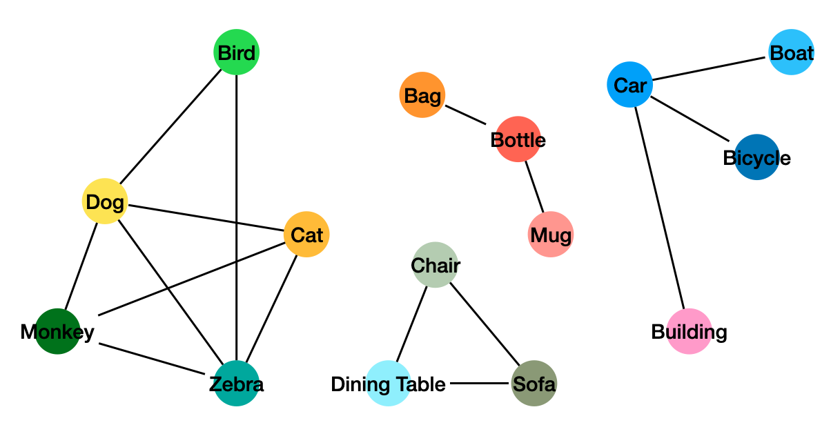
Figure 3: The graphical ontology generated for aPY data set.

4.4 Evaluating Clustering Performance

Here we report if the descriptive clustering problem can increase clustering quality. Since these methods are not deep learning based, to make a fair comparison we use the same pre-trained ResNet-101 features. We report the clustering results of our model under a range of annotated ratios in Table 3. We have several observations to highlight: firstly our model consistently outperforms the k-means and multi-view clustering baselines with different tag annotated ratios; secondly with more annotated tags, both multi-view clustering baselines and our model improves largely comparing to the k-means clustering which naively concatenates the images features with semantic attributes. We attribute the good clustering performance for both deep representation learning and our novel way of leveraging semantic tag information for better clustering.

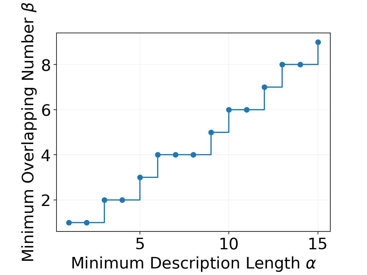
(a) Parameter analysis on $\alpha$

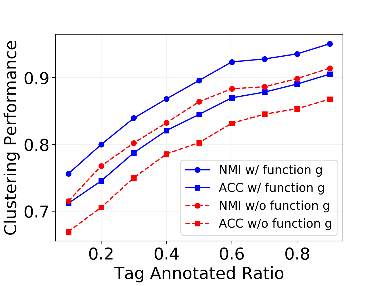
(b) Ablation study on function $g$

Figure 4: Plots for parameter analysis and ablation study

4.5 Parameter Analysis and Ablation Test

Given the hyper-parameter $\alpha$ which denotes the minimum expected number of tags for description, we plot the automatically searched parameter $\beta$ for AwA in Figure 4 (a). This result shows our automatic searching procedure’s success and suggests that a relatively small $\alpha$ leads to more concise and orthogonal explanations. Meanwhile, we conduct ablation experiments to analyze the impact of mask function $g$ solved via our explanation module. In Figure 4 (b), the blue lines indicate clustering results with function $g$. In red lines we replace function $g$ with an identity function to conduct the ablation study. Comparing red and blue lines we can see that mask function $g$ can remove the noisy information within semantic tag space and consistently improve the clustering performance.

5 Conclusion and Future Work

This paper proposes deep descriptive clustering, which can learn to cluster and generate cluster-level explanations simultaneously. We develop a novel deep learning framework that supports learning from the sub-symbolic level (which clustering is performed on) and symbolic level (which explanations are created from). Empirical results on real-world data demonstrate the high quality of our generated explanations and good clustering performance. Our future work will focus on building an explainable clustering model with noisy semantic features and exploring other novel forms of explanations beyond ontologies on different types of data.

References

- Adadi and Berrada [2018] Amina Adadi and Mohammed Berrada. Peeking inside the black-box: A survey on explainable artificial intelligence (xai). IEEE Access, 6:52138–52160, 2018.
- Basu et al. [2008] Sugato Basu, Ian Davidson, and Kiri Wagstaff. Constrained clustering: Advances in algorithms, theory, and applications. CRC Press, 2008.
- Bertsimas et al. [2020] Dimitris Bertsimas, Agni Orfanoudaki, and Holly Wiberg. Interpretable clustering: an optimization approach. Machine Learning, pages 1–50, 2020.
- Bickel and Scheffer [2004] S Bickel and T Scheffer. Multi-view clustering. In Fourth IEEE International Conference on Data Mining (ICDM’04), pages 19–26. IEEE, 2004.
- Bilenko et al. [2004] Mikhail Bilenko, Sugato Basu, and Raymond J Mooney. Integrating constraints and metric learning in semi-supervised clustering. In Proceedings of the twenty-first international conference on Machine learning, page 11, 2004.
- Bridle et al. [1992] John S Bridle, Anthony JR Heading, and David JC MacKay. Unsupervised classifiers, mutual information and’phantom targets. In Advances in neural information processing systems, pages 1096–1101, 1992.
- Dao et al. [2018] Thi-Bich-Hanh Dao, Chia-Tung Kuo, SS Ravi, Christel Vrain, and Ian Davidson. Descriptive clustering: Ilp and cp formulations with applications. In Proceedings of the 27th International Joint Conference on Artificial Intelligence, pages 1263–1269, 2018.
- Davidson et al. [2018] Ian Davidson, Antoine Gourru, and S Ravi. The cluster description problem-complexity results, formulations and approximations. Advances in Neural Information Processing Systems, 31:6190–6200, 2018.
- Farhadi et al. [2009] Ali Farhadi, Ian Endres, Derek Hoiem, and David Forsyth. Describing objects by their attributes. In 2009 IEEE Conference on Computer Vision and Pattern Recognition, pages 1778–1785. IEEE, 2009.
- Fogel et al. [2019] Sharon Fogel, Hadar Averbuch-Elor, Daniel Cohen-Or, and Jacob Goldberger. Clustering-driven deep embedding with pairwise constraints. IEEE computer graphics and applications, 39(4):16–27, 2019.
- Fraiman et al. [2013] Ricardo Fraiman, Badih Ghattas, and Marcela Svarc. Interpretable clustering using unsupervised binary trees. Advances in Data Analysis and Classification, 7(2):125–145, 2013.
- Ghattas et al. [2017] Badih Ghattas, Pierre Michel, and Laurent Boyer. Clustering nominal data using unsupervised binary decision trees: Comparisons with the state of the art methods. Pattern Recognition, 67:177–185, 2017.
- He et al. [2016] Kaiming He, Xiangyu Zhang, Shaoqing Ren, and Jian Sun. Deep residual learning for image recognition. In Proceedings of the IEEE conference on computer vision and pattern recognition, pages 770–778, 2016.
- Hu and Chen [2018] Menglei Hu and Songcan Chen. Doubly aligned incomplete multi-view clustering. In Proceedings of the 27th International Joint Conference on Artificial Intelligence, pages 2262–2268, 2018.
- Kingma and Ba [2015] Diederik P Kingma and Jimmy Ba. Adam: A method for stochastic optimization. In International Conference on Learning Representations, 2015.
- Krause et al. [2010] Andreas Krause, Pietro Perona, and Ryan Gomes. Discriminative clustering by regularized information maximization. Advances in neural information processing systems, 23:775–783, 2010.
- Lampert et al. [2013] Christoph H Lampert, Hannes Nickisch, and Stefan Harmeling. Attribute-based classification for zero-shot visual object categorization. IEEE transactions on pattern analysis and machine intelligence, 36(3):453–465, 2013.
- Liu et al. [2005] Bing Liu, Yiyuan Xia, and Philip S Yu. Clustering via decision tree construction. In Foundations and advances in data mining, pages 97–124. Springer, 2005.
- Moshkovitz et al. [2020] Michal Moshkovitz, Sanjoy Dasgupta, Cyrus Rashtchian, and Nave Frost. Explainable k-means and k-medians clustering. In International Conference on Machine Learning, pages 7055–7065. PMLR, 2020.
- Ribeiro et al. [2016] Marco Tulio Ribeiro, Sameer Singh, and Carlos Guestrin. ” why should i trust you?” explaining the predictions of any classifier. In Proceedings of the 22nd ACM SIGKDD international conference on knowledge discovery and data mining, pages 1135–1144, 2016.
- Sambaturu et al. [2020] Prathyush Sambaturu, Aparna Gupta, Ian Davidson, S. S. Ravi, Anil Vullikanti, and Andrew Warren. Efficient algorithms for generating provably near-optimal cluster descriptors for explainability. Proceedings of the AAAI Conference on Artificial Intelligence, 34:1636–1643, Apr. 2020.
- Shao et al. [2015] Weixiang Shao, Lifang He, and S Yu Philip. Multiple incomplete views clustering via weighted nonnegative matrix factorization with regularization. In Joint European Conference on Machine Learning and Knowledge Discovery in Databases, pages 318–334. Springer, 2015.
- Strehl et al. [2000] Alexander Strehl, Joydeep Ghosh, and Raymond Mooney. Impact of similarity measures on web-page clustering. In Workshop on artificial intelligence for web search (AAAI 2000), volume 58, page 64, 2000.
- Tao et al. [2017] Zhiqiang Tao, Hongfu Liu, Sheng Li, Zhengming Ding, and Yun Fu. From ensemble clustering to multi-view clustering. In Proceedings of the 26th International Joint Conference on Artificial Intelligence, pages 2843–2849, 2017.
- Wagstaff et al. [2001] Kiri Wagstaff, Claire Cardie, Seth Rogers, Stefan Schrödl, et al. Constrained k-means clustering with background knowledge. In International Conference on Machine Learning, volume 1, pages 577–584, 2001.
- Wang et al. [2018] Yang Wang, Lin Wu, Xuemin Lin, and Junbin Gao. Multiview spectral clustering via structured low-rank matrix factorization. IEEE transactions on neural networks and learning systems, 29(10):4833–4843, 2018.
- Xu et al. [2003] Wei Xu, Xin Liu, and Yihong Gong. Document clustering based on non-negative matrix factorization. In Proceedings of the 26th annual international ACM SIGIR conference on Research and development in informaion retrieval, pages 267–273, 2003.
- Xu et al. [2013] Chang Xu, Dacheng Tao, and Chao Xu. A survey on multi-view learning. arXiv preprint arXiv:1304.5634, 2013.
- Zhang et al. [2019] Hongjing Zhang, Sugato Basu, and Ian Davidson. A framework for deep constrained clustering-algorithms and advances. In Joint European Conference on Machine Learning and Knowledge Discovery in Databases, pages 57–72. Springer, 2019.
- Zhao et al. [2016] Handong Zhao, Hongfu Liu, and Yun Fu. Incomplete multi-modal visual data grouping. In Proceedings of the Twenty-Fifth International Joint Conference on Artificial Intelligence, pages 2392–2398, 2016.