Shearing approach to gauge invariant Trotterization

Abstract

Universal quantum simulations of gauge field theories are exposed to the risk of gauge symmetry violations when it is not known how to compile the desired operations exactly using the available gate set. In this letter, we show how time evolution can be compiled in an Abelian gauge theory—if only approximately—without compromising gauge invariance, by graphically motivating a block-diagonalization procedure. When gauge invariant interactions are associated with a “spatial network” in the space of discrete quantum numbers, it is seen that cyclically shearing the spatial network converts simultaneous updates to many quantum numbers into conditional updates of a single quantum number: ultimately, this eliminates any need to pass through (and acquire overlap onto) unphysical intermediate configurations. Shearing is explicitly applied to gauge-matter and magnetic interactions of lattice QED. The features that make shearing successful at preserving Abelian gauge symmetry may also be found in non-Abelian theories, bringing one closer to gauge invariant simulations of quantum chromodynamics.

The real-time dynamics of quantum field theories (QFTs) holds the details of rich nonperturbative physics, such as the fragmentation of jets at the Large Hadron Collider or early-universe bubble nucleation in extensions of the Standard Model. Analytic methods that can quantitatively predict nonperturbative phenomena from the underlying quantum field theories are scarce, and this deficit underlies the existence of what is today a sophisticated, numerical lattice QFT program. For decades, the lattice QFT program has pushed the envelope of high-performance computing and fundamental physics, but its scope has generally been restricted to properties for which a QFT’s Euclidean or imaginary-time path integral is not hampered by a sign problem. The calculation of real-time dynamics has largely been precluded by sign problems, except for special cases [luscherVolumeDependence86, luscherTwoparticleStates91]. The fact is that real-time dynamics explicitly involves events in Minkowskian, rather than Euclidean, spacetime. Any general computational solution—if one exists—will require the use of nontraditional lattice methods.

In recent years, a new computational avenue for dynamics has opened up [martinez.muschik.eaRealtimeDynamics16, klco.dumitrescu.eaQuantumclassicalComputation18, kokail.othersSelfverifyingVariational19, schweizer.grusdt.eaFloquetApproach19, klco.savage.eaSUNonAbelian20, yang.sun.eaObservationGauge20, kreshchuk.jia.eaLightFrontField20, klco.savageMinimallyEntangled20, gustafson.zhu.eaRealtimeQuantum21, bauer.freytsis.eaSimulatingCollider21, atas.zhang.eaSUHadrons21, rahman.lewis.eaSULattice21, ciavarella.klco.eaTrailheadQuantum21a] based on simulating field theoretic degrees of freedom [jordan.lee.eaQuantumAlgorithms12, jordan.lee.eaQuantumComputation14, bhattacharyya.shekar.eaCircuitComplexity18, klco.savageDigitizationScalar19, klco.savageSystematicallyLocalizable20, barata.mueller.eaSingleparticleDigitization21, cirac.maraner.eaColdAtom10, casanova.lamata.eaQuantumSimulation11, jordan.lee.eaQuantumAlgorithms14, hamedmoosavian.jordanFasterQuantum18, nuqscollaboration.lamm.eaPartonPhysics20, mueller.tarasov.eaDeeplyInelastic20a, harmalkar.lamm.eaQuantumSimulation20, kharzeev.kikuchiRealtimeChiral20, nachman.provasoli.eaQuantumAlgorithm21, davoudi.linke.eaSimulatingQuantum21, banuls.blatt.eaSimulatingLattice20, byrnes.yamamotoSimulatingLattice06, strykerOraclesGauss19, nuqscollaboration.lamm.eaGeneralMethods19, nuqscollaboration.alexandru.eaGluonField19, zohar.ciracRemovingStaggered19, shaw.lougovski.eaQuantumAlgorithms20a, chakraborty.honda.eaDigitalQuantum20, liu.xinQuantumSimulation20, paulson.dellantonio.eaSimulating2D20, nuqscollaboration.ji.eaGluonField20, davoudi.raychowdhury.eaSearchEfficient20, bender.zoharGaugeRedundancyfree20a, haase.dellantonio.eaResourceEfficient21, kan.funcke.eaInvestigating1D21, zohar.reznikConfinementLattice11, zohar.cirac.eaQuantumSimulations13, zohar.burrelloFormulationLattice15, zohar.farace.eaDigitalQuantum17, bender.zohar.eaDigitalQuantum18, davoudi.hafezi.eaAnalogQuantum20, mil.zache.eaScalableRealization20, banerjee.dalmonte.eaAtomicQuantum12, tagliacozzo.celi.eaOpticalAbelian13, mezzacapo.rico.eaNonAbelianSU15, zache.hebenstreit.eaQuantumSimulation18, zohar.cirac.eaColdAtomQuantum13, mathur.sreerajLatticeGauge16, raychowdhury.strykerLoopString20, raychowdhury.strykerSolvingGauss20, dasgupta.raychowdhuryColdAtom20, kreshchuk.kirby.eaQuantumSimulation20, buser.gharibyan.eaQuantumSimulation20] and their interactions with laboratory-controllable quantum systems, i.e., quantum simulators and computers [feynmanSimulatingPhysics82, lloydUniversalQuantum96]. Quantum computers are naturally suited for simulating Hamiltonian mechanics, as opposed to path integrals, and thereby appear to be sign problem-free. This letter is specifically concerned with simulation by universal digital quantum computers (as opposed to analog ones, as well as quantum annealers), which are the model for architectures like those being engineered by Google [arute.arya.eaQuantumSupremacy19], IBM [chow.gambetta.eaUniversalQuantum12], IonQ [debnath.linke.eaDemonstrationSmall16], Rigetti [reagor.osborn.eaDemonstrationUniversal18], and others.

Digital quantum simulation requires a quantum algorithm or set of instructions to be executed by the quantum computer. For QFTs, this may entail truncating and mapping the field degrees of freedom onto quantum bits (qubits) and mimicking Schrödinger-picture time evolution through an appropriate sequence of unitary gates. At the end of the evolution, measurements would be made to extract the observables of interest. How exactly QFTs and their dynamics would best be “digitized” is a subject of active research [wieseQuantumSimulating14, zohar.farace.eaDigitalLattice17, kaplan.strykerGaussLaw20, klco.savageDigitizationScalar19, nuqscollaboration.lamm.eaGeneralMethods19, nuqscollaboration.alexandru.eaGluonField19, raychowdhury.strykerLoopString20, klco.savage.eaSUNonAbelian20, davoudi.raychowdhury.eaSearchEfficient20, bender.zoharGaugeRedundancyfree20a, meurice.sakai.eaTensorField20, kreshchuk.kirby.eaQuantumSimulation20, barata.mueller.eaSingleparticleDigitization21, nachman.provasoli.eaQuantumAlgorithm21, bauer.freytsis.eaSimulatingCollider21, ciavarella.klco.eaTrailheadQuantum21a].

Among field theories that will be studied by quantum computers, gauge theories such as quantum chromodynamics are uniquely complex due to their hallmark local constraints — namely gauge invariance, which is identified with Gauss’s law and charge conservation. Unlike certain analog devices, in which there can be opportunities to map gauge symmetry to a physical symmetry of the simulator [zohar.cirac.eaColdAtomQuantum13], qubits and the operations done on them generally do not discriminate between gauge-violating interactions and gauge-conserving ones. Gauge symmetry, therefore, is a concern for both the wave functions and the effectively simulated interactions. We do note, however, that there is evidence of dynamical robustness against gauge-violating interactions in certain contexts [tran.su.eaFasterDigital21, halimeh.haukeStaircasePrethermalization20]. Unless these observations can be extended to and made rigorous for more general gauge theories (particularly in the continuum limit), manifestly gauge invariant protocols, where possible and practical, remain preferable.

Symmetry preservation aside, a crucial consideration in selecting any QFT digitization is the implementation of its time evolution. Gauge theory Hamiltonians are often given in the form $H=\sum_{j}H_{j}$, where each $H_{j}$ is a manifestly gauge invariant operator involving fields from a site, link, or unit square (plaquette) of a spatial lattice. The time evolution operator $e^{-itH}$ generally will not be a native operation and must be constructed from the available gate set. The simplest and most well-studied approaches take advantage of Lie-Trotter-Suzuki product formulas [trotterProductSemigroups59, suzukiGeneralizedTrotter76, childs.su.eaTheoryTrotter21]: at first order, $e^{-i\,tH}\simeq\left[\prod_{j}e^{-i\,tH_{j}/s}\right]^{s}$ for a sufficiently large number of Trotter steps, $s$. This Trotterization of the time evolution operator is inexact for finite $s$, but it is gauge invariant because each $H_{j}$ is.

In practice, the complexity of the $H_{j}$ may call for a second level of approximation: $e^{-i\,\delta tH_{j}}\rightarrow\prod_{k}V_{jk}(\delta t)$ in the limit of small $\delta t$, where each factor $V_{jk}(\delta t)$ is an implementable sequence of elementary gates. There is no reason to expect a priori that the individual $V_{jk}$ will be gauge invariant, nor is there any guarantee $\prod_{k}V_{jk}(\delta t)$ conserves gauge symmetry either. Protecting gauge invariance through this second layer of approximation (which is also referred to as Trotterization) is a nontrivial aspect of designing the quantum circuit.

In this letter, a solution is introduced for Trotterizing Abelian gauge theories while preserving gauge symmetry. This is achieved by finding collections $V_{jk}(\delta t)$ that are individually gauge invariant, implying gauge invariant time evolution. The key insight is that the transitions induced by gauge invariant operators can be thought of as a geometric graph or “spatial network” of parallel edges. Through appropriate changes of basis, the edges can be aligned parallel to the axis of a single quantum number, effectively turning the problem of tightly correlated transitions of multiple quantum numbers into transitions of a single quantum number conditioned by Boolean logic. This method, based on ‘cyclic shears,’ is illustrated by applying it to hopping terms (minimally-coupled fermion-photon interactions) and plaquette operators encountered in compact U(1) gauge theories, such as lattice QED.

U(1) hopping terms.—In Ref. [shaw.lougovski.eaQuantumAlgorithms20a], complete and scalable algorithms with bounded errors were given for time evolution of the lattice Schwinger model (QED in 1D space), truncated in the basis of electric fields and fermion occupation numbers. The $H_{j}$ were link-localized electric energies and hopping terms, and site-localized mass terms. The propagators $e^{-itH_{j}/s}$ associated to the electric and mass terms could be decomposed straightforwardly and exactly using typical universal gate sets because they are diagonal in the computational basis. The off-diagonal hopping terms do not enjoy the same benefit, making it less obvious how to exactly decompose their associated propagators as circuits.

Concretely, let $\hat{\psi}$ and $\hat{\chi}$ be the fermionic modes at two neighboring lattice sites, $\hat{U}$ the gauge link variable joining them, $x>0$ the interaction strength, and $\hat{T}_{\text{hop}}=x\,\hat{\psi}^{\dagger}\hat{\chi}\hat{U}$ the associated hopping term. Conjugate to a link operator is the integer electric field $\hat{E}$ along that link; we work in the eigenbasis of $\hat{E}$, with $\hat{U}=\sum_{E}\ket{E+1}\bra{E}$. We also assume a hard cutoff for which $E_{\text{min}}\leq E\leq E_{\text{max}}$ and $\hat{U}\ket{E_{\text{max}}}=\hat{U}^{\dagger}\ket{E_{\text{min}}}=0$.

A Jordan-Wigner transformation can be used to turn the fermionic operators into qubit (spin $\tfrac{1}{2}$) operators, e.g., ^T_hop = x   σ^-_ψσ^+_χ^U ; we are using a computational basis in which $\sigma^{+}=\ket{0}\bra{1}$ and 0 and 1 denote eigenvalues of $\hat{n}_{\psi}\equiv\hat{\psi}^{\dagger}\hat{\psi}$ or $\hat{n}_{\chi}\equiv\hat{\chi}^{\dagger}\hat{\chi}$. Electric eigenstates, truncated to $\eta$ qubits per link, are interchangeably labelled by nonnegative integers $\mathcal{E}=E-E_{\text{min}}$. Arithmetic involving $\hat{\mathcal{E}}$ is always modulo $2^{\eta}$.

In multiqubit quantum computation, it is common for Pauli operator to refer to any tensor product of Pauli matrices $I$, $X$, $Y$, or $Z$ acting on individual qubit spaces (e.g., $X\otimes X$ or $I\otimes Z\otimes Z$). Pauli operators form a Hermitian basis for all multiqubit operators. The expression of an operator with respect to this basis is its Pauli decomposition. The exponential of a Pauli operator is considered easy to simulate, but directly Trotterizing the Pauli decomposition can be prohibitively inefficient. Generally, one will divide up and manipulate different parts of the Hamiltonian before arriving at Pauli operators intended for hardware implementation.

Diagonalized operators such as $\hat{E}^{2}$ in the Schwinger model are trivial to program without approximation because Trotterizing their Pauli decomposition incurs no commutation errors: $[I,Z]=0$. The off-diagonal hopping terms, however, are not as trivial to implement exactly, in part due to $[X,Y]\neq 0$. Diagonalizing the involved field operators is not an option since they are nilpotent. The fields’ Hermitian and antihermitian parts are of course diagonalizable, but they are not by themselves gauge covariant and they fail to commute. Ref. [shaw.lougovski.eaQuantumAlgorithms20a] went forward with the Hermitian and antihermitian fields, postponing the construction of fully gauge invariant Trotter steps.

Insight into the computational nature of gauge invariant transitions can be gained by graphically examining the structure of hopping terms as a whole within the space of quantum numbers. The top panel of Fig. 1 depicts the transitions induced by $\hat{T}_{\text{hop}}$ and $\hat{T}_{\text{hop}}^{\dagger}$ as edges in the $(n_{\psi},n_{\chi},E)$ space of quantum numbers (shown for $\eta=2$).

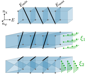
Figure 1: Graphical representation of the transitions induced by hopping terms. Top: The transitions before any change of basis. Middle: The transitions after $\hat{\xi}_{1}$. Bottom: The transitions after $\hat{\xi}_{2}\hat{\xi}_{1}$.

An edge connecting $(n_{\psi}^{i},n_{\chi}^{i},E^{i})$ and $(n_{\psi}^{f},n_{\chi}^{f},E^{f})$ corresponds to a nonzero matrix element $\langle n_{\psi}^{f},n_{\chi}^{f},E^{f}|(\hat{T}_{\text{hop}}+\hat{T}_{\text{hop}}^{\dagger})|n_{\psi}^{i},n_{\chi}^{i},E^{i}\rangle$. The transitions form what is known in graph theory as a geometric graph or spatial network. This particular spatial network consists of parallel edges whose slant represents simultaneous changes to all three relevant quantum numbers – as given, hopping terms are off-diagonal on all three field registers.

If the edges were instead oriented parallel to one of the axes, the interaction would be off-diagonal on a single register only. Such a block-diagonalization would make it easier to avoid most gauge-violating transitions by simply excluding all $X$ and $Y$ operations on the other registers’ qubits. It is clear from Fig. 1 that this scenario is entirely attainable by appropriately shearing the graph.

The middle section of Fig. 1 show the result of a ‘cyclic shear’ transformation, which is mathematically given by ^ξ_1 &= δ_ ^n_ψ, 0 + δ_ ^n_ψ, 1 ^λ^-  ,
^ξ_1 ^T_hop ^ξ_1^†= x   σ^-_ψσ^+_χ( 1 - δ_ ^E , E_max )  . Above, $\delta$s serve as shorthand for projection operators: $\delta_{\hat{n}_{\psi},0}=(\ket{0}\bra{0})_{\psi}$, $\delta_{\hat{E},E_{\text{max}}}=\ket{E_{\text{max}}}\bra{E_{\text{max}}}$, etc. We also introduce cyclic incrementers $\hat{\lambda}^{\pm}=\sum_{\mathcal{E}=0}^{2^{\eta}-1}\ket{\mathcal{E}\pm 1}\bra{\mathcal{E}}$. The ‘cyclicity’ of the shear transformation thus means that when a node gets sheared beyond the extent of its range, it wraps around to the opposite boundary and continues being sheared. In this way, the shears provide unitary mappings that can be applied to computational basis states.

Under $\hat{\xi}_{1}$, $\hat{T}_{\text{hop}}$ becomes off-diagonal on two registers only. This can then be combined with another shear, ^ξ_2 &= δ_ ^n_ψ, 0 + δ_ ^n_ψ, 1 X_χ ,
^ξ_2 ( ^ξ_1 ^T_hop ^ξ_1^†) ^ξ_2^†= x   δ_ ^n_χ, 1 σ^-_ψ( 1 - δ_ ^E , E_max )  . After the combined transformation $\hat{\xi}_{2}\hat{\xi}_{1}$, $\hat{T}_{\text{hop}}$ becomes off-diagonal on the space of a single qubit. The projector $(1-\delta_{\hat{E},E_{\text{max}}})$ that has arisen is necessary to prevent a reduced set of possible gauge-violating errors: those that correspond to wrap-around effects at the cutoffs. This is the work left to be done by hand, as far as charge conservation is concerned.

Fortuitously, in this case of gauge-fermion hopping terms, the work left to be done by hand is negligible. The Hermitian operator to be simulated, $\delta_{\hat{n}_{\chi},1}X_{\psi}(1-\delta_{\hat{E},E_{\text{max}}})$, can be implemented with two controlled $X$-rotations. Figure 2 shows these gates sandwiched between the shears. This circuit, which was only tailor-made to conserve charge, is actually an exact gate decomposition for the hopping propagator.

[row sep=0.5cm,between origins,column sep=.35cm] $\ket{n_{\psi}}$ & [label position=above] ^ξ_1 2 [label position=above] ^ξ_2 1 e^-i   x   δt X e^i   x   δt X [label position=above] ^ξ_2^† 1 [label position=above] ^ξ_1^† 2
$\ket{n_{\chi}}$ -1-1
$\ket{\mathcal{E}}$ ^λ^- [alternate] [alternate][alternate]-1[alternate] ^λ^+ [alternate] [alternate]

Figure 2: Circuit to simulate a gauge-fermion hopping term $x(\hat{\psi}^{\dagger}\hat{\chi}\hat{U}-\hat{\psi}\hat{\chi}^{\dagger}\hat{U}^{\dagger})$. The multiqubit electric register could be any number of qubits.

Compact U(1) plaquettes.—The shearing of plaquettes is explained below by first considering a toy model, two-link ‘plaquette’: two links joined end to end. The toy plaquette highlights every key feature of solving plaquette operators using shears, but is more easily visualized than the case of four links. The generalization to the four-link plaquette is summarized thereafter.

Consider two links labeled ‘1’ and ‘2’ with their truncated ‘plaquette’ operator given by ^U_1 ^U_2^†&= ^λ_1^+ [ 1 - δ_ ^E_1 , E_max ] ^λ_2^- [ 1 - δ_ ^E_2 , E_min ]
= ^λ_1^+ ^λ_2^- [ 1 - δ_ ^E_1 , -1 ] [ 1 - δ_ ^E_2 , 0 ]  . A consequence of $[\hat{U}_{1}\hat{U}_{2}^{\dagger},\hat{E}_{1}+\hat{E}_{2}]=0$ is that the electric configurations that can be mixed by $\hat{U}_{1}\hat{U}_{2}^{\dagger}$ lie on various one-dimensional lines in the space of electric quantum numbers. As illustrated in Fig. LABEL:fig:toyShear, these transitions can be aligned with one axis by a shear in the 12-plane: ^Ξ_12 &≡∑_j=0^2^η- 1 δ_^E_1, j ( ^λ_2^+ )^j  . Computationally, $\hat{\Xi}_{12}$ is nothing but addition modulo $2^{\eta}$: $\ket{\mathcal{E}_{1}}\ket{\mathcal{E}_{2}}\overset{\Xi_{12}}{\rightarrow}\ket{\mathcal{E}_{1}}\ket{\mathcal{E}_{2}+\mathcal{E}_{1}}$. Applying $\hat{\Xi}_{12}$ to the operators appearing in (2), we find that $\hat{\lambda}_{2}^{-}$ and $\hat{\mathcal{E}}_{1}$ are invariant, whereas $\hat{\lambda}_{1}^{+}\overset{\Xi_{12}}{\rightarrow}\hat{\lambda}_{1}^{+}\hat{\lambda}_{2}^{+}$ and $\hat{\mathcal{E}}_{2}\overset{\Xi_{12}}{\rightarrow}\hat{\mathcal{E}}_{2}-\hat{\mathcal{E}}_{1}$. Therefore ^Ξ