Heat Distribution of Relativistic Brownian Motion

Abstract

Understanding the statistical behavior of the heat in stochastic systems gives us insight about the thermodynamics of such systems. Using the recently proposed Relativistic Stochastic Thermodynamics, we investigate the statistics of the heat of a Relativistic Ornstein-Uhlenbeck particle, comparing with the classical cases. The results are exact through numerical integration of the Fokker-Planck of the joint distribution, and are validated by numerical simulations.

Keywords: heat fluctuations; stochastic thermodynamics; relativistic brownian motion.

I Introduction

Understanding the behavior of the heat exchanged by a system has always had an important role in physics. Since the beginnings of thermodynamics, understanding how a system loses or gains energy from the surroundings was important to develop early thermal machines carnot2012reflections . With today’s technological advances, we are able to thermodynamically interact on an increasingly smaller scale, ranging from micrometer to nanometer. Typically, these systems are far from equilibrium, where the thermodynamics’s functionals, such as heat, entropy, or work, are treated as fluctuating quantities. The field of the investigations of the thermodynamics of such fluctuating systems is well known in the literature as the Stochastic Thermodynamics oliveira2020classical ; ciliberto_experiments_2017 ; seifert2012stochastic ; sekimoto2010stochastic .

Heat is a fundamental quantity in Stochastic Thermodynamics, i.e., the energy naturally exchanged between the system and the surrounding, in a disordered way. As a random variable, characterization of the statistics of heat for diffusive systems was carried in many different models paraguassu_heat_2021_2 ; paraguassu_heat_2021 ; gupta_heat_2021 ; fogedby_heat_2020 ; goswami_heat_2019 ; crisanti_heat_2017 ; ghosal_distribution_2016 ; rosinberg_heat_2016 ; kim_heat_2014 ; kusmierz_heat_2014 ; saha_work_2014 ; chatterjee_single-molecule_2011 ; chatterjee_exact_2010 ; fogedby_heat_2009 ; imparato_probability_2008 ; imparato_work_2007 ; joubaud_fluctuation_2007 . These works bring physical insights into the thermodynamics of classical diffusive systems, however, as far as we known, they only deals with non-relativistic systems.

Relativistic diffusive systems are expected to be found in nature, and can appear in quite different phenomena such as cosmic jets pal_stochastic_2020 ; meyer2018cosmic , quark-muon plasma produced by heavy ion collisions koide_thermodynamic_2011 ; akamatsu_heavy_2009 , and graphene in a semiclassical regime  pototsky_relativistic_2012 ; pototsky_periodically_2013 . From a more mathematical point of view, these relativistic diffusive systems can be modeled by the Relativistic Brownian motion dunkel_theory_2005 ; dunkel_theory_2005-1 ; dunkel_relativistic_2009 which are a particular case of Brownian motion with nonlinear friction term lindner_diffusion_2007 . One well studied case is the Relativistic Orstein-Uhlenbeck debbasch_relativistic_1997 , where its relaxation properties were studied in debbasch_thermal_2012 ; felderhof_momentum_2012 .

Recently, Pal and Deffner proposed a Stochastic Thermodynamic framework for the Relativistic Brownian motion pal_stochastic_2020 . Their model is based on the Relativistic Ornstein-Uhlenbeck case, where they define heat, work, and entropy for the relativistic Brownian particle. This relativistic version of classical Stochastic thermodynamics quantities sekimoto2010stochastic was shown to satisfy the conservation of energy and the fluctuation theorem version of the second law of thermodynamics. Since heat is a fundamental quantity, we thus want to understand its behavior for this new relativistic case. It is meaningful to check if the relativistic stochastic thermodynamics leads to a consistent statistical behavior of the heat. Moreover, it is also interesting to compare with the classical case. How different is the behavior of the heat between the classical and relativistic system? In addition, it is important to notice, that the same definition of heat was also proposed by Koide and Kodama in koide_thermodynamic_2011 .

In the present paper, by means of the Stochastic Thermodynamics framework pal_stochastic_2020 , we investigate the heat distribution for the Relativistic Ornstein-Uhlenbeck model. We obtain the heat distribution in two distinct limits, the exact relativity limit, and the ultra-relativistic limit. The results are exact through numerical integration. We use the variational formula for the Fokker-Planck langtangen2016solving ; risken1996fokker , and we integrate it numerically. We also use the Path integral formalism onsager1953fluctuations ; moreno_conditional_2019 ; wio2013path ; chaichian2018path to deal with the ultra-relativistic case. The results are compared with numerical simulations of the stochastic process and are found in agreement.

The paper is organized as follows: In section II we define the model and its thermodynamics. In section III we studied the heat fluctuations of the relativistic case by path integrals. In section IV we obtain, through numerical integration of the Fokker-Planck equation of the joint distribution. We conclude in section V with a discussion of the results.

II Relativistic Orstein-Uhlenbeck

As a first model to study the heat fluctuations of a relativistic particle, we study the free case, often called Relativistic Ornstein-Uhlenbeck dunkel_relativistic_2009 . Despite being the most simple situation for the relativistic Brownian particle, we will see that the non-linear dependency on the momentum can lead us to non-trivial results.

A relativistic particle is a particle with an absolute velocity not exceeding the speed of light $|V(t)|<c$. Its stochastic behavior for the momentum is defined in the inertial frame of the environment and the corresponding stochastic equation is (unless explicitly stated, we assume $c=1$)

$$dp=-\Gamma(p)dt+\sqrt{2\gamma MT}dW_{t},$$ (1)

where

$$\Gamma(p)=\gamma M\frac{p}{\sqrt{p^{2}+M^{2}}}=\gamma MV(t),$$

is the nonlinear drift term of the relativistic Orstein-Uhlenbeck model debbasch_relativistic_1997 , and $V(t)=p/\sqrt{p^{2}+M^{2}}<1$ is the relativistic velocity of the particle. Writing in terms of the absolute velocity, the interpretation of the drift term is simple: it is just the drift $-\gamma V$, but now with the velocity constrained by $V<c$.

For $M\gg p$ we find the classical case, while for $p\gg M$ we have the ultra-relativistic limit, where the velocity of the particle is close to the speed of light. The constants above are: the drift $\gamma$, the temperature of the surrounding $T$, and the rest mass of the particle $M$. The integrated noise $dW_{t}$ is a delta-correlated Wiener process wio2013path , and models the fast degrees of freedom of the environment. According to koide_thermodynamic_2011 ; pal_stochastic_2020 the heat functional is given by

$$Q[p(t)] = \int_{0}^{t}\frac{p}{\sqrt{p^{2}+M^{2}}}\left(-\Gamma(p)+\sqrt{2\gamma MT}dW_{\tau}\right)d\tau$$ (2)

$$= \sqrt{p_{t}^{2}+M^{2}}-\sqrt{p_{0}^{2}+M^{2}},$$

where $Q<0$ means that the particle is losing energy to the environment, while $Q>0$ says that the particle is absorbing energy from the environment. The balance of energy is the same as for the classical case. The drift term is responsible for the negatives values, while the noise term yields positive values. What changes, comparing with the non-relativistic case, is the non-trivial dependence on $p$ in the drift term. Notice that the first law of thermodynamics in the absence of work, i.e., $Q[p]=\Delta E$, is valid since $E=\sqrt{p^{2}+M^{2}}$ is the relativistic energy.

We assume that the particle is initially in thermal equilibrium with the environment, with initial distribution given by the Juttner distribution cubero_thermal_2007

$$\rho(p_{0},0)=\rho_{0}\exp\left(-\beta\sqrt{p^{2}+M^{2}}\right),$$ (3)

which is the correct equilibrium thermal distribution of the Relativistic Orstein-Uhlenbeck model, as verified by a microscopic collision simulation in cubero_thermal_2007 .

II.1 Heat Functional

The heat, being a functional of the trajectory, has the conditional probability

$$P(Q|Q=Q[p])=\delta(Q-Q[p]).$$ (4)

It emphasizes that the random values of $Q$ are given by the trajectory-dependent formula $Q[p]$. In the studied case, the heat only depends on the initial and final points of the trajectory. Therefore, the probability distribution for the heat will be given by

$$P(Q,t) = \int dp_{t}dp_{0}\rho(p_{0})\int_{p(0)=p_{0}}^{p(t)=p_{t}}Dpe^{-\mathcal{A}[p]}\delta(Q-Q[p(t)])$$ (5)

$$= \int dp_{t}P(Q,p_{t},t),$$

where the path integral is over all the possible continuous non-differentiable trajectories chaichian2018path and $\mathcal{A}[p(t)]$ is the stochastic action (see Appendix).

III Ultra-relativistic Regime

The ultra-relativistic regime occurs when the Brownian particle has a speed close to $c$, or equivalently $p\gg M$. In this regime the energy is given by a linear dependency in the momentum. As a consequence, the equation for the particle’s momentum will be simplified. Interestingly, it has been shown that the ultra-relativistic Brownian motion, can describe the behavior of the charge carriers on a graphene plate pototsky_relativistic_2012 ; pototsky_periodically_2013 where, instead of the constant $c$, we have the Fermi velocity $v_{f}$. The analysis presented here can be cast as a simplified version of such a system as well.

In the ultra-relativistic regime, $E=c|p|$ and the Langevin equation becomes

$$dp=-\gamma c\;\frac{p}{|p|}dt+\sqrt{2\gamma T}dW_{t},$$ (6)

where the drift term is now similar to a dry friction force pototsky_periodically_2013 ; gennes_brownian_2005 . Notice that $c$ is no longer equals one here. (Because we don’t have mass, it is important to use another parameter in the equations.) Following the definitions given in section II, the heat exchanged between the particle and the environment will be

$$Q[p]=\Delta E=c(|p_{t}|-|p_{0}|),$$ (7)

which is the first law of Stochastic Thermodynamics koide_thermodynamic_2011 ; pal_stochastic_2020 . The heat distribution is then given by

$$P(Q)=\int dp_{t}\int dp_{0}\rho(p_{0})P[p_{t},t|p_{0}]\delta(Q-Q[p]),$$ (8)

where we remove the Dirac delta of the path integral in Eq. 5, making the path integral become the conditional probability. The conditional probability is written in as a path integral wio2013path ; moreno_conditional_2019

$$P[p_{t},t|p_{0}]=\int^{p(t)=p_{t}}_{p(0)=p_{0}}Dp\;e^{-\mathcal{A}[p(t)]},$$ (9)

which is a sum over all trajectories that are continuous and non-differentiable chaichian2018path . The result of this path integral is

$$P[p_{t},t|p_{0}]=\frac{e^{-\frac{c}{2T}\left(-|p_{0}|+|p_{t}|+\frac{c\gamma t}{2}\right)}}{\int P[p_{t},t|p_{0}]dp_{t}}\left(\frac{c}{8T}e^{\frac{c}{4T}\left(\frac{c\gamma t}{4}-(|p_{0}|+|p_{t}|)\right)}\left(\text{erf}\left(\frac{c\gamma t-2(|p_{0}|+|p_{t}|)}{4\sqrt{\gamma tT}}\right)+1\right)+\frac{e^{-\frac{(p_{t}-p_{0})^{2}}{4\gamma tT}}}{2\sqrt{\gamma T\pi t}}\right),$$ (10)

where erf is the error function. We derive the above result in Appendix A. This conditional probability can be checked by numerical simulations of the Langevin Eq. 6. We can rewrite the Dirac delta to find a more convenient formula for the heat distribution

$$P(Q)=\int\frac{d\lambda}{2\pi}e^{i\lambda Q}Z(\lambda),$$ (11)

where

$$Z(\lambda)=\int dp_{t}\int dp_{0}\rho(p_{0})e^{-i\lambda c(|p_{t}|-|p_{0}|)}P[p_{t},t|p_{0}],$$ (12)

is the characteristic function of the heat, where we use the Juttner initial equilibrium distribution $\rho(p_{0})=\rho_{0}\exp(-\beta c|p_{0}|)$. Due to the complicated dependence on $p_{0}$, $Z(\lambda)$ cannot be solved analytically. We find $Z(\lambda)$ by numerically integrating over $p_{t}$ and $p_{0}$. The result is plotted in Fig.1. Notice that $Z(0)=1$, meaning that the distribution is properly normalized. Given $Z(\lambda)$ we use Eq. 11 to numerically integrate over $\lambda$ and find the heat distribution. The distribution is plotted in Fig. 2 a).

The heat distribution in Fig. 2 a) is symmetrical, meaning that the particle has no tendency to absorb or lose energy from the bath. This behavior is encountered in its classical version, where $\Gamma(p)=-\gamma\frac{p}{M}$. It happens because we start in thermal equilibrium using the Juttner distribution. Moreover, compared with the classical case, the distribution is smoother around $Q=0$, meaning that, for a given trajectory, the chance for the particle absorbing or losing energy is larger than the classical case paraguassu_heat_2021_2 .

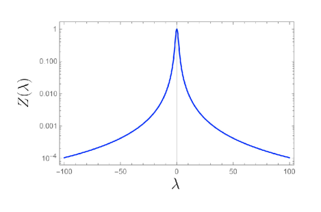
Figure 1: Characteristic function of the heat in $t=1$. Note that $Z(0)=1$. All constants are set to one.

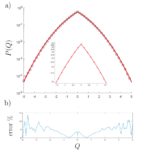
Figure 2: a) Heat distribution for the ultra-relativistic particle at time $t=1$. The inset figure is the heat distribution in the small interval $[-1.5,1.5]$ . The solid red line is the theoretical solution, while the open circles are the numerical simulation b) Relative error in $P(Q)$ between simulation and solution. All constants are set to 1.

IV Exact Solution

To solve the model exactly, a path integral technique can only give us an approximate result. Thus, we opt to use the Fokker-Planck formalism, which can be solved by numerical integration. We also compare the Fokker-Planck result with numerical simulations of the Langevin equation. The stochastic equation for the momentum is

$$dp=-\gamma M\frac{p}{\sqrt{p^{2}+M^{2}}}dt+\sqrt{2\gamma MT}dW_{t}.$$ (13)

The joint heat distribution $P(Q,p)$ can be solved exactly via the Fokker-Planck equation. One such approach was used in the derivation of the heat and work distributions of a Brownian particle in a double well potential imparato_work_2007 ; imparato_probability_2008 . One considers the stochastic equation for the heat

$$dQ=\frac{p}{\sqrt{p^{2}+M^{2}}}dp=$$

$$=-\gamma M\frac{p^{2}}{p^{2}+M^{2}}dt+\frac{p}{\sqrt{p^{2}+M^{2}}}\sqrt{2\gamma MT}dW_{t},$$ (14)

where we replaced $dp$ by the Langevin equation Eq. 13. With the above equation we can construct the Fokker-Planck for the joint distribution $P(Q,p)$. The Fokker-Planck for $P(Q,p)$ and its initial condition are

$$\frac{\partial}{\partial t}P(Q,p)=-\nabla\cdot\left(\vec{F}P(Q,p)-\bm{B}\cdot\nabla P(Q,p)\right),$$

$$P(Q,p,t=0)=\delta(Q)\rho(p_{0}),$$ (15)

where $\nabla=\left(\partial_{p},\partial_{Q}\right)$, and

$$\vec{F}=\begin{pmatrix}\frac{-\gamma Mp}{\sqrt{p^{2}+M^{2}}}\\ \frac{-\gamma Mp^{2}}{p^{2}+M^{2}}\end{pmatrix},\;\;\;\bm{B}=\begin{pmatrix}2\gamma MT&\frac{2\gamma MTp}{\sqrt{p^{2}+M^{2}}}\\ \frac{2\gamma MTp}{\sqrt{p^{2}+M^{2}}}&\frac{2\gamma MTp^{2}}{p^{2}+M^{2}}.\end{pmatrix}$$ (16)

Eq. 15 can be solved numerically giving $P(Q,p)$ which can be integrated numerically over $p$ to give the heat distribution $P(Q)$. We solve Eq. 15 numerically through the Finite Elements method logg2012automated , implemented by FEniCS langtangen2016solving , which uses the variational formula of the PDE, also know as the weak form logg2012automated . In our case, the variational formula is

$$\int\partial_{t}P(Q,p)\;vd\Sigma=$$

$$=\int\vec{F}\cdot\nabla vP(Q,p)d\Sigma-\int\bm{B}\nabla P(Q,p)\cdot\nabla vd\Sigma,$$ (17)

where $v$ is a test function, and we are integrating in the domain $d\Sigma=dpdQ$. In this variational formula, the boundary condition in the weak form is satisfied by

$$\oint(-\vec{F}P+\bm{B}\cdot\nabla P(Q,p))\cdot\hat{n}v\;d\partial\Sigma=0$$ (18)

which ensures the no flux boundary conditions over the integrated region. We implement the time evolution by an Euler scheme. The result $P(Q,p)$ is plotted in Fig. 3. With $P(Q,p)$ we integrate it numerically over $p$, obtaining the heat distribution $P(Q)$ plotted in Fig. 4 a). The relative error between the Fokker-Planck solution and the numerical simulation is in Fig. 4 c), showing the agreement between the two approaches.

The behavior of the heat distribution is clear. The particle in average will not absorb or gain energy from the environment and it is equally probable to lose or to gain energy since the distribution is symmetrical. This shows that the system is naturally close to equilibrium, which is expected since we assume an initially thermalized distribution. Moreover, comparing with the ultra-relativistic case, we see a peak around $Q=0$ meaning that the tendency of zero average heat is stronger than for the ultra-relativistic case.

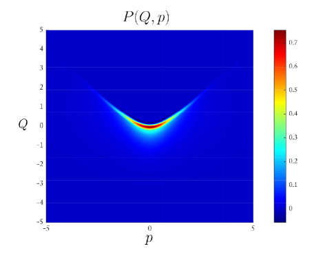
Figure 3: a) Joint distribution $P(Q,p)$. Note the shape of the curve obeys a behavior of $\sim\sqrt{(p^{2}+1)}$, which comes from the definition of heat. All constants are set to one.

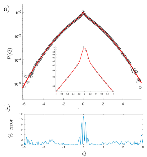
Figure 4: a) Heat distribution in time $t=1$. Note the peak behavior in $Q=0$ a feature common in many stochastic thermodynamics systems. The inset figure is the heat distribution in the small interval $[-1,1]$. The red solid line is the Fokker-Planck result, while the open circles are the simulation of the Langevin equation. b) Relative error between simulation and numerical solution. All constants are set to one.

V Conclusion

In the present paper, we have study the energy exchanged between a Relativistic diffusive particle and a thermal environment. We solve for the heat distribution in two different regimes, the ultra-relativistic and the exact relativistic limit. We first calculate the heat distribution for the ultra-relativistic limit through the use of path integrals. We find exact results through numerical integration of the characteristic function. For the exact limit, such an approach is not available, thus we use FEniCS langtangen2016solving to numerically solve the Fokker-Planck of the joint distribution $P(Q,p)$, and then integrate over $p$ to find $P(Q)$. Both results are in essence exact and agree with numerical simulations.

Physically, we find that in the Relativistic Stochastic Thermodynamics the heat shares similar statistical behavior compared with the classical (non-relativistic) case paraguassu_heat_2021_2 (see also rosinberg_stochastic_2017 ; munakata_entropy_2012 ). The relativistic heat distribution for the free particle has a sharp distribution around $Q=0$, meaning that the particle neither absorbs nor gains energy on average from the environment. This result is also consistent with the classical case. Moreover, another similarity is the symmetry of the distribution, which is $P(Q)=P(-Q)$ showing that there is no preferred direction for the heat. One can expect this result since no external force or internal potential is interacting with the particle. Therefore, the proposed Relativistic Stochastic Thermodynamics leads to well-behaved physical properties for the heat.

The methods presented here can be generalized to higher dimensions, which is a more realistic scenario. A promising case is in the graphene chip pototsky_relativistic_2012 , wherre the charge carriers could obey the 2D Ultra-relativistic Langevin equation. Thus, one can study the protocols in the ultra-relativistic case, performing work on the system, and even study thermal machines protocols. Hence, the present study can also serve as a starting point to the study of such machines. By calculating the heat, and work distribution, one can investigate the efficiency of such a case. This will be a theme of future work.

Moreover, a more realistic scenario can also take into account interactions and multiplicative noise plyukhin_quasirelativistic_2013 . Both complications can also be treated with the methods exposed herein.

Appendix A Path integral for Ultra-relativistic case

In equation 10 the conditional probability can be derived by means of path integral technique. Which states that

$$P[p_{t},t|p_{0}]=\int^{p(t)=p_{t}}_{p(0)=p_{0}}Dp\;e^{-\mathcal{A}[p(t)]}$$ (19)

where $\mathcal{A}[p(t)]$ is the stochastic action wio2013path ; chaichian2018path ; moreno_conditional_2019 , in the Stratonovich prescription is given by

$$\mathcal{A}[p(t)]=\frac{1}{4D}\int_{0}^{t}\left(\dot{p}+\gamma c\frac{p}{|p|}\right)^{2}d\tau-\frac{\gamma c}{2}\int_{0}^{t}\frac{\partial}{\partial p}\frac{p}{|p|}d\tau,$$ (20)

where $D=\gamma T$. By noticing that $p/|p|=\text{sign}(p)=2H(p)-1$ and $H^{\prime}(p)=\delta(p)$, we can rewrite the action as

$$\mathcal{A}[p(t)]=\frac{1}{4D}\int_{0}^{t}\left(\dot{p}^{2}-\alpha\delta(p)\right)d\tau+\frac{\gamma c}{2D}\left(\frac{\gamma c}{2}t+|p_{t}|-|p_{0}|\right)$$ (21)

where, $\alpha=4D\gamma c$. The conditional probability can be rewritten as

$$P[p_{t},t|p_{0}]=e^{-\frac{\gamma c}{2D}\left(\frac{\gamma c}{2}t+|p_{t}|-|p_{0}|\right)}K[p_{t},t|p_{0}],$$ (22)

where $K[p_{t},t|p_{0}]$ will be the path integral

$$K[p_{t},t|p_{0}]=\int^{p(t)=p_{t}}_{p(0)=p_{0}}Dp\exp\left(-\frac{1}{4D}\int_{0}^{t}\left(\dot{p}^{2}-\alpha\delta(p)\right)d\tau\right)$$ (23)

which has the same structure of a quantum mechanical propagator of a particle with a delta potential blinder_greens_1988 ; crandall_combinatorial_1993 ; goovaerts_new_1973 ; lawande_feynman_1988 . Thus, following lawande_feynman_1988 we review the derivation of this path integral.

To solve Eq. 23 we expand the potential, obtaining

$$K[p_{t},t|p_{0}]=K_{0}[p_{t},t|p_{0}]+K_{1}[p_{t},t|p_{0}]$$ (24)

where

$$K_{0}[p_{t},t|p_{0}]=\int^{p(t)=p_{t}}_{p(0)=p_{0}}Dpe^{-\frac{1}{4D}\int\dot{p}^{2}d\tau}=\frac{1}{\sqrt{4\pi Dt}}e^{-\frac{p_{t}^{2}}{4Dt}},$$ (25)

$$K_{1}[p_{t},t|p_{0}]=\sum_{n=1}^{\infty}\left(\frac{-1}{4D}\right)^{n}\frac{(-\alpha)^{n}}{n!}\int Dp\;e^{-\frac{1}{4D}\int\dot{p}^{2}d\tau}\left(\int_{0}^{t}\delta(p)d\tau\right)^{n}.$$ (26)

Therefore, we only have to solve $K_{1}$. To do this, note that

$$\left(\int_{0}^{t}\delta(p)d\tau\right)^{n}=\int_{0}^{t}dt_{n}\int_{0}^{t}dt_{n-1}\dots\int_{0}^{t}dt_{2}\int_{0}^{t}dt_{1}\prod_{k=1}^{n}\delta(p(t_{k}))$$ (27)

$$=n!\int_{0}^{t}dt_{n}\int_{0}^{t_{n}}dt_{n-1}\dots\int_{0}^{t_{2}}dt_{1}\prod_{k=1}^{n}\delta(p(t_{k}))$$ (28)

where in the second line, we just reordered the time. The path integral in $K$ is a Wiener path integral that describes a Markovian stochastic process, thus we have the property

$$K_{0}[p_{t},t|p_{0}]=K_{0}[p_{t},t|p_{n},t_{n}]K_{0}[p_{n},t_{n}|p_{n-1},t_{n-1}]\dots K_{0}[p_{1},t_{1}|p_{0},0],$$ (29)

therefore, in $K_{1}$ we have

$$\int dp_{n}\int dp_{n-1}\dots\int dp_{1}K_{0}[p_{t},t|p_{n},t_{n}]\delta(p_{n})\prod_{k=2}^{n}K_{0}[p_{k},t_{k}|p_{k-1}t_{k-1}]K_{0}[p_{1},t_{1}|p_{0},0]\delta(p_{k})\delta(p_{1})=$$ (30)

$$=K_{0}[p_{t},t|0,t_{n}]\prod_{k=2}^{n}K_{0}[0,t_{k}|0,t_{k-1}]K_{0}[0,t_{1}|p_{0},0].$$ (31)

Thus, we have

$$K_{1}=\sum_{n=1}^{\infty}\left(\frac{\alpha}{4D}\right)^{n}\int_{0}^{t}dt_{n}\int_{0}^{t_{n}}dt_{n-1}\dots\int_{0}^{t_{2}}dt_{1}K_{0}[p_{t},t|0,t_{n}]\prod_{k=2}^{n}K_{0}[0,t_{k}|0,t_{k-1}]K_{0}[0,t_{1}|p_{0},0].$$ (32)

Note that we have convolutions between the propagators. Then, by making the Laplace’s transform

$$\tilde{K}_{1}=\int_{0}^{\infty}e^{st}K_{1}[p_{t},t|p_{0}],$$ (33)

we can get rid of the time integrals, giving

$$\tilde{K}_{1}=\sum_{n=1}^{\infty}\left(\frac{\alpha}{4D}\right)^{n}\tilde{K}(p_{t},s)\tilde{K}(0,s)^{n-1}\tilde{K}(p_{0},s)$$ (34)

where

$$\tilde{K}(p,s)=\int_{0}^{\infty}e^{st}\frac{e^{-\frac{p^{2}}{4Dt}}}{\sqrt{4\pi Dt}}=\exp\left({-|p|\sqrt{\frac{s}{D}}}\right)\sqrt{\frac{1}{4\pi Ds}},$$ (35)

then

$$\tilde{K}_{1}=\sum_{n=1}^{\infty}\left(\frac{\gamma c}{\sqrt{4D}}\right)^{n}\exp\left({-(|p_{t}|+|p_{0}|)\sqrt{\frac{s}{D}}}\right)\left[\sqrt{\frac{1}{s}}\right]^{n+1}.$$ (36)

The above sum is solved exactly, and then, we can use the inverse Laplace transform to find the desired $K_{1}$.

$$K_{1}[p_{t},t|p_{0}]=\frac{c\gamma}{2\pi i}\int_{\gamma-i\infty}^{\gamma+i\infty}\frac{\exp\left({-(|p_{t}|+|p_{0}|)\sqrt{\frac{s}{D}}}+st\right)}{\sqrt{sD}(2\sqrt{sD}-\gamma c)}ds$$ (37)

we can make $s=w^{2}$, giving

$$K_{1}[p_{t},t|p_{0}]=\frac{c\gamma}{i\pi\sqrt{D}}\int_{C}\frac{\exp\left({-(|p_{t}|+|p_{0}|)\sqrt{\frac{1}{D}}w}+w^{2}t\right)}{(2\sqrt{D}w-\gamma c)}dw$$ (38)

rewriting the denominator as an integral

$$K_{1}[p_{t},t|p_{0}]=\frac{c\gamma}{i\pi\sqrt{D}}\int_{0}^{\infty}\int_{C}{\exp\left({-(|p_{t}|+|p_{0}|)\sqrt{\frac{1}{D}}w}+w^{2}t+z(2\sqrt{D}w-\gamma c)\right)}dwdz$$ (39)

This allow us to solve the integral in $w$ as a gaussian integral, giving

$$K_{1}[p_{t},t|p_{0}]=\frac{c\gamma}{\sqrt{\pi t}}\int_{0}^{\infty}e^{\frac{z\gamma c}{4D}}e^{-\frac{(z+\xi)^{2}}{4Dt}}dz,$$ (40)

where $\xi=|p_{t}|+|p_{0}|$. We finally have

$$K_{1}[p_{t},t|p_{0}]=\frac{\gamma c}{8D}e^{\frac{\gamma c}{4D}\left(\frac{c\gamma t}{4}-\xi\right)}\left(\text{erf}\left(\frac{c\gamma t-2\xi}{4\sqrt{Dt}}\right)+1\right).$$ (41)

Finally, with Eq. 41 and 25 we have the conditional probability

$$P[p_{t},t|p_{0}]=e^{-\frac{c}{2T}\left(-|p_{0}|+|p_{t}|+\frac{c\gamma t}{2}\right)}\left(\frac{\gamma c}{8D}e^{\frac{c}{4T}\left(\frac{c\gamma t}{4}-\xi\right)}\left(\text{erf}\left(\frac{c\gamma t-2\xi}{4\sqrt{Dt}}\right)+1\right)+\frac{e^{-\frac{(p_{t}-p_{0})^{2}}{4Dt}}}{2\sqrt{D\pi t}}\right),$$ (42)

which can be normalized, giving Eq. 4.

References

References

- (1) Carnot S 2012 Reflections on the motive power of fire: And other papers on the second law of thermodynamics (Courier Corporation)
- (2) Oliveira M J d 2020 Revista Brasileira de Ensino de Física 42
- (3) Ciliberto S 2017 Phys. Rev. X 7 021051 publisher: American Physical Society URL https://link.aps.org/doi/10.1103/PhysRevX.7.021051
- (4) Seifert U 2012 Reports on progress in physics 75 126001
- (5) Sekimoto K 2010 Stochastic energetics vol 799 (Springer)
- (6) Paraguassú P V, Aquino R and Morgado W A M 2021 arXiv:2102.09115 [cond-mat] ArXiv: 2102.09115 URL http://arxiv.org/abs/2102.09115
- (7) Paraguassú P V and Morgado W A M 2021 J. Stat. Mech. 2021 023205 ISSN 1742-5468 publisher: IOP Publishing URL https://doi.org/10.1088/1742-5468/abda25
- (8) Gupta D and Sivak D A 2021 arXiv:2103.09358 [cond-mat] ArXiv: 2103.09358 URL http://arxiv.org/abs/2103.09358
- (9) Fogedby H C 2020 J. Stat. Mech. 2020 083208 ISSN 1742-5468 publisher: IOP Publishing URL https://doi.org/10.1088/1742-5468/aba7b2
- (10) Goswami K 2019 Phys. Rev. E 99 012112 publisher: American Physical Society URL https://link.aps.org/doi/10.1103/PhysRevE.99.012112
- (11) Crisanti A, Sarracino A and Zannetti M 2017 Phys. Rev. E 95 052138 publisher: American Physical Society URL https://link.aps.org/doi/10.1103/PhysRevE.95.052138
- (12) Ghosal A and Cherayil B J 2016 J. Stat. Mech. 2016 043201 ISSN 1742-5468 publisher: IOP Publishing URL https://doi.org/10.1088/1742-5468/2016/04/043201
- (13) Rosinberg M L, Tarjus G and Munakata T 2016 EPL 113 10007 ISSN 0295-5075 publisher: IOP Publishing URL https://doi.org/10.1209/0295-5075/113/10007
- (14) Kim K, Kwon C and Park H 2014 Phys. Rev. E 90 032117 ISSN 1539-3755, 1550-2376 URL https://link.aps.org/doi/10.1103/PhysRevE.90.032117
- (15) Kuśmierz \, Rubi J M and Gudowska-Nowak E 2014 J. Stat. Mech. 2014 P09002 ISSN 1742-5468 publisher: IOP Publishing URL https://doi.org/10.1088/1742-5468/2014/09/p09002
- (16) Saha B and Mukherji S 2014 J. Stat. Mech. 2014 P08014 ISSN 1742-5468 URL https://iopscience.iop.org/article/10.1088/1742-5468/2014/08/P08014
- (17) Chatterjee D and Cherayil B J 2011 J. Stat. Mech. 2011 P03010 ISSN 1742-5468 URL https://iopscience.iop.org/article/10.1088/1742-5468/2011/03/P03010
- (18) Chatterjee D and Cherayil B J 2010 Phys. Rev. E 82 051104 ISSN 1539-3755, 1550-2376 URL https://link.aps.org/doi/10.1103/PhysRevE.82.051104
- (19) Fogedby H C and Imparato A 2009 J. Phys. A: Math. Theor. 42 475004 ISSN 1751-8121 publisher: IOP Publishing URL https://doi.org/10.1088/1751-8113/42/47/475004
- (20) Imparato A, Jop P, Petrosyan A and Ciliberto S 2008 J. Stat. Mech. 2008 P10017 ISSN 1742-5468 URL https://iopscience.iop.org/article/10.1088/1742-5468/2008/10/P10017
- (21) Imparato A, Peliti L, Pesce G, Rusciano G and Sasso A 2007 Phys. Rev. E 76 050101 publisher: American Physical Society URL https://link.aps.org/doi/10.1103/PhysRevE.76.050101
- (22) Joubaud S, Garnier N B and Ciliberto S 2007 J. Stat. Mech. 2007 P09018–P09018 ISSN 1742-5468 publisher: IOP Publishing URL https://doi.org/10.1088/1742-5468/2007/09/p09018
- (23) Pal P S and Deffner S 2020 New J. Phys. 22 073054 ISSN 1367-2630 URL https://iopscience.iop.org/article/10.1088/1367-2630/ab9ce6
- (24) Meyer E T 2018 Nature Astronomy 2 32–33
- (25) Koide T and Kodama T 2011 Phys. Rev. E 83 061111 ISSN 1539-3755, 1550-2376 URL https://link.aps.org/doi/10.1103/PhysRevE.83.061111
- (26) Akamatsu Y, Hatsuda T and Hirano T 2009 Phys. Rev. C 79 054907 ISSN 0556-2813, 1089-490X URL https://link.aps.org/doi/10.1103/PhysRevC.79.054907
- (27) Pototsky A, Marchesoni F, Kusmartsev F V, Hänggi P and Savel’ev S E 2012 Eur. Phys. J. B 85 356 ISSN 1434-6028, 1434-6036 URL http://link.springer.com/10.1140/epjb/e2012-30716-7
- (28) Pototsky A and Marchesoni F 2013 Phys. Rev. E 87 032132 ISSN 1539-3755, 1550-2376 URL https://link.aps.org/doi/10.1103/PhysRevE.87.032132
- (29) Dunkel J and Hänggi P 2005 Phys. Rev. E 71 016124 ISSN 1539-3755, 1550-2376 URL https://link.aps.org/doi/10.1103/PhysRevE.71.016124
- (30) Dunkel J and Hänggi P 2005 Phys. Rev. E 72 036106 ISSN 1539-3755, 1550-2376 URL https://link.aps.org/doi/10.1103/PhysRevE.72.036106
- (31) Dunkel J and Hänggi P 2009 Physics Reports 471 1–73 ISSN 03701573 URL https://linkinghub.elsevier.com/retrieve/pii/S0370157308004171
- (32) Lindner B 2007 New J. Phys. 9 136–136 ISSN 1367-2630 URL https://iopscience.iop.org/article/10.1088/1367-2630/9/5/136
- (33) Debbasch F, Mallick K and Rivet J P 1997 Journal of Statistical Physics 88 945–966 ISSN 1572-9613 URL https://doi.org/10.1023/B:JOSS.0000015180.16261.53
- (34) Debbasch F, Espaze D, Foulonneau V and Rivet J P 2012 Physica A: Statistical Mechanics and its Applications 391 3797–3804 ISSN 03784371 URL https://linkinghub.elsevier.com/retrieve/pii/S0378437112001732
- (35) Felderhof B U 2012 Phys. Rev. E 86 061103 ISSN 1539-3755, 1550-2376 URL https://link.aps.org/doi/10.1103/PhysRevE.86.061103
- (36) Langtangen H P and Logg A 2016 Solving PDEs in python: the FEniCS tutorial I (Springer Nature)
- (37) Risken H 1996 Fokker-planck equation The Fokker-Planck Equation (Springer) pp 63–95
- (38) Onsager L and Machlup S 1953 Physical Review 91 1505
- (39) Moreno M V, Barci D G and Arenas Z G 2019 Phys. Rev. E 99 032125 ISSN 2470-0045, 2470-0053 URL https://link.aps.org/doi/10.1103/PhysRevE.99.032125
- (40) Wio H S 2013 Path integrals for stochastic processes: An introduction (World Scientific)
- (41) Chaichian M and Demichev A 2018 Path integrals in physics: Volume I stochastic processes and quantum mechanics (CRC Press)
- (42) Cubero D, Casado-Pascual J, Dunkel J, Talkner P and Hänggi P 2007 Phys. Rev. Lett. 99 170601 ISSN 0031-9007, 1079-7114 URL https://link.aps.org/doi/10.1103/PhysRevLett.99.170601
- (43) Gennes P G d 2005 J Stat Phys 119 953–962 ISSN 0022-4715, 1572-9613 URL http://link.springer.com/10.1007/s10955-005-4650-4
- (44) Logg A, Mardal K A and Wells G 2012 Automated solution of differential equations by the finite element method: The FEniCS book vol 84 (Springer Science & Business Media)
- (45) Rosinberg M L, Tarjus G and Munakata T 2017 Phys. Rev. E 95 022123 ISSN 2470-0045, 2470-0053 URL https://link.aps.org/doi/10.1103/PhysRevE.95.022123
- (46) Munakata T and Rosinberg M L 2012 J. Stat. Mech. 2012 P05010 ISSN 1742-5468 publisher: IOP Publishing URL https://iopscience.iop.org/article/10.1088/1742-5468/2012/05/P05010/meta
- (47) Plyukhin A V 2013 Phys. Rev. E 88 052115 ISSN 1539-3755, 1550-2376 URL https://link.aps.org/doi/10.1103/PhysRevE.88.052115
- (48) Blinder S M 1988 Phys. Rev. A 37 973–976 publisher: American Physical Society URL https://link.aps.org/doi/10.1103/PhysRevA.37.973
- (49) Crandall R E 1993 J. Phys. A: Math. Gen. 26 3627–3648 ISSN 0305-4470 publisher: IOP Publishing URL https://doi.org/10.1088/0305-4470/26/14/024
- (50) Goovaerts M J, Babcenco A and Devreese J T 1973 Journal of Mathematical Physics 14 554–559 ISSN 0022-2488 publisher: American Institute of Physics URL https://aip.scitation.org/doi/10.1063/1.1666355
- (51) Lawande S V and Bhagwat K V 1988 Physics Letters A 131 8–10 ISSN 0375-9601 URL https://www.sciencedirect.com/science/article/pii/0375960188906226