A new computational framework for log-concave density estimation

Abstract

In Statistics, log-concave density estimation is a central problem within the field of nonparametric inference under shape constraints. Despite great progress in recent years on the statistical theory of the canonical estimator, namely the log-concave maximum likelihood estimator, adoption of this method has been hampered by the complexities of the non-smooth convex optimization problem that underpins its computation. We provide enhanced understanding of the structural properties of this optimization problem, which motivates the proposal of new algorithms, based on both randomized and Nesterov smoothing, combined with an appropriate integral discretization of increasing accuracy. We prove that these methods enjoy, both with high probability and in expectation, a convergence rate of order $1/T$ up to logarithmic factors on the objective function scale, where $T$ denotes the number of iterations. The benefits of our new computational framework are demonstrated on both synthetic and real data, and our implementation is available in a github repository LogConcComp (Log-Concave Computation).

1 Introduction

In Statistics, the field of nonparametric inference under shape constraints dates back at least to Grenander, (1956), who studied the nonparametric maximum likelihood estimator of a decreasing density on the non-negative half line. But it is really over the last decade or so that researchers have begun to realize its full potential for addressing key contemporary data challenges such as (multivariate) density estimation and regression. The initial allure is the flexibility of a nonparametric model, combined with estimation methods that can often avoid the need for tuning parameter selection, which can often be troublesome for other nonparametric techniques such as those based on smoothing. Intensive research efforts over recent years have revealed further great attractions: for instance, these procedures frequently attain optimal rates of convergence over relevant function classes. Moreover, it is now known that shape-constrained procedures can possess intriguing adaptation properties, in the sense that they can estimate particular subclasses of functions at faster rates, even (nearly) as well as the best one could do if one were told in advance that the function belonged to this subclass.

Typically, however, the implementation of shape-constrained estimation techniques requires the solution of an optimization problem, and, despite some progress, there are several cases where computation remains a bottleneck and hampers the adoption of these methods by practitioners. In this work, we focus on the problem of log-concave density estimation, which has become arguably the central challenge in the field because the class of log-concave densities enjoys stability properties under marginalization, conditioning, convolution and linear transformations that make it a very natural infinite-dimensional generalization of the class of Gaussian densities (Samworth,, 2018).

The univariate log-concave density estimation problem was first studied in Walther, (2002), and fast algorithms for the computation of the log-concave maximum likelihood estimator (MLE) in one dimension are now available through the R packages logcondens (Dümbgen and Rufibach,, 2011) and cnmlcd (Liu and Wang,, 2018). Cule et al., (2010) introduced and studied the multivariate log-concave maximum likelihood estimator, but their algorithm, which is described below and implemented in the R package LogConcDEAD (Cule et al.,, 2009), is slow; for instance, Cule et al., (2010) report a running time of 50 seconds for computing the bivariate log-concave MLE with 500 observations, and 224 minutes for computing the log-concave MLE in four dimensions with 2,000 observations. An alternative, interior point method for a suitable approximation was proposed by Koenker and Mizera, (2010). Recent progress on theoretical aspects of the computational problem in the computer science community includes Axelrod et al., (2019), who proved that there exists a polynomial time algorithm for computing the log-concave maximum likelihood estimator. We are unaware of any attempt to implement this algorithm. Rathke and Schnörr, (2019) compute an approximation to the log-concave MLE by considering $-\log p$ as a piecewise affine maximum function, using the log-sum-exp operator to approximate the non-smooth operator, a Riemann sum to compute the integral and its gradient, and obtain a solution via L-BFGS. This reformulation means that the problem is no longer convex.

To describe the problem more formally, let $\mathcal{C}_{d}$ denote the class of proper, convex lower-semicontinuous functions $\varphi:\mathbb{R}^{d}\rightarrow(-\infty,\infty]$ that are coercive in the sense that $\varphi(\bm{x})\rightarrow\infty$ as $\|\bm{x}\|\rightarrow\infty$. The class of upper semi-continuous log-concave densities on $\mathbb{R}^{d}$ is denoted as

$$\mathcal{P}_{d}:=\biggl{\{}p:\mathbb{R}^{d}\rightarrow[0,\infty):p=e^{-\varphi}\text{ for some }\varphi\in\mathcal{C}_{d},\int_{\mathbb{R}^{d}}p=1\biggr{\}}.$$

Given $\bm{x}_{1},\ldots,\bm{x}_{n}\in\mathbb{R}^{d}$, Cule et al., (2010, Theorem 1) proved that whenever the convex hull $C_{n}$ of $\bm{x}_{1},\ldots,\bm{x}_{n}$ is $d$-dimensional, there exists a unique

$$\hat{p}_{n}\in\operatorname*{argmax}_{p\in\mathcal{P}_{d}}\frac{1}{n}\sum_{i=1}^{n}\log p(\bm{x}_{i}).$$ (1)

If $\bm{x}_{1},\ldots,\bm{x}_{n}$ are regarded as realizations of independent and identically distributed random vectors on $\mathbb{R}^{d}$, then the objective function in (1) is a scaled version of the log-likelihood function, so $\hat{p}_{n}$ is called the log-concave MLE. The existence and uniqueness of this estimator is not obvious, because the infinite-dimensional class $\mathcal{P}_{d}$ is non-convex, and even the class of negative log-densities $\bigl{\{}\varphi\in\mathcal{C}_{d}:\int_{\mathbb{R}^{d}}e^{-\varphi}=1\bigr{\}}$ is non-convex. In fact, the estimator belongs to a finite-dimensional subclass; more precisely, for a vector $\bm{\phi}=(\phi_{1},\ldots,\phi_{n})\in\mathbb{R}^{n}$, define $\mathrm{cef}[\bm{\phi}]\in\mathcal{C}_{d}$ to be the (pointwise) largest function with

$$\mathrm{cef}[\bm{\phi}](\bm{x}_{i})\leq\phi_{i}$$

for $i=1,\ldots,n$. Cule et al., (2010) proved that $\hat{p}_{n}=e^{-\mathrm{cef}[\bm{\phi}^{*}]}$ for some $\bm{\phi}^{*}\in\mathbb{R}^{n}$, and refer to the function $-\mathrm{cef}[\bm{\phi}^{*}]$ as a ‘tent function’; see the illustration in Figure 1. Cule et al., (2010) further defined the non-smooth, convex objective function $f:\mathbb{R}^{n}\rightarrow\mathbb{R}$ by

$$f(\bm{\phi})\equiv f(\phi_{1},\ldots,\phi_{n}):=\frac{1}{n}\sum_{i=1}^{n}\phi_{i}+\int_{C_{n}}\exp\bigl{\{}-\mathrm{cef}[\bm{\phi}](x)\bigr{\}}\,dx,$$ (2)

and proved that $\bm{\phi}^{*}=\operatorname*{argmin}_{\bm{\phi}\in\mathbb{R}^{n}}f(\bm{\phi})$.

Figure 1: An illustration of a tent function, taken from Cule et al., (2010).

The two main challenges in optimizing the objective function $f$ in (2) are that the value and subgradient of the integral term are hard to evaluate, and that it is non-smooth, so vanilla subgradient methods lead to a slow rate of convergence. To address the first issue, Cule et al., (2010) computed the exact integral and its subgradient using the qhull algorithm (Barber et al.,, 1993) to obtain a triangulation of the convex hull of the data, evaluating the function value and subgradient over each simplex in the triangulation. However, in the worst case, the triangulation can have $O(n^{d/2})$ simplices (McMullen,, 1970). The non-smoothness is handled via Shor’s $r$-algorithm (Shor,, 1985, Chapter 3), as implemented by Kappel and Kuntsevich, (2000).

In Section 2, we characterize the subdifferential of the objective function in terms of the solution of a linear program (LP), and show that the solution lies in a known, compact subset of $\mathbb{R}^{n}$. This understanding allows us to introduce our new computational framework for log-concave density estimation in Section 3, based on an accelerated version of a dual averaging approach (Nesterov,, 2009). This relies on smoothing the objective function, and encompasses two popular strategies, namely Nesterov smoothing (Nesterov,, 2005) and randomized smoothing (Lakshmanan and De Farias,, 2008; Yousefian et al.,, 2012; Duchi et al.,, 2012), as special cases. A further feature of our algorithm is the construction of approximations to gradients of our smoothed objective, and this in turn requires an approximation to the integral in (2). While a direct application of the theory of Duchi et al., (2012) would yield a rate of convergence for the objective function of order $n^{1/4}/T+1/\sqrt{T}$ after $T$ iterations, we show in Section 4 that by introducing finer approximations of both the integral and its gradient as the iteration number increases, we can obtain an improved rate of order $1/T$, up to logarithmic factors. Moreover, we translate the optimization error in the objective into a bound on the error in the log-density, which is uncommon in the literature in the absence of strong convexity. A further advantage of our approach is that we are able to extend it in Section 5 to the more general problem of quasi-concave density estimation (Koenker and Mizera,, 2010; Seregin and Wellner,, 2010), thereby providing a computationally tractable alternative to the discrete Hessian approach of Koenker and Mizera, (2010). Section 6 illustrates the practical benefits of our methodology in terms of improved computational timings on simulated data. Additional experimental details and applications on real data sets are provided in Appendix A. Proofs of all main results can be found in Appendix B, and background on the field of nonparametric inference under shape constraints can be found in Appendix C.

Notation:

We write $[n]:=\{1,2,\ldots,n\}$, let $\bm{1}\in\mathbb{R}^{n}$ denote the all-ones vector, and denote the cardinality of a set $S$ by $|S|$. For a Borel measurable set $C\subseteq\mathbb{R}^{d}$, we use $\mathrm{vol}(C)$ to denote its volume (i.e. $d$-dimensional Lebesgue measure). We write $\|\cdot\|$ for the Euclidean norm of a vector. For $\mu>0$, a convex function $f:\mathbb{R}^{n}\rightarrow\mathbb{R}$ is said to be $\mu$-strongly convex if $\bm{\phi}\mapsto f(\bm{\phi})-\frac{\mu}{2}\|\bm{\phi}\|^{2}$ is convex. The notation $\partial f(\bm{\phi})$ denotes the subdifferential (set of subgradients) of $f$ at $\bm{\phi}$. Given a real-valued sequence $(a_{n})$ and a positive sequence $(b_{n})$, we write $a_{n}=\tilde{O}(b_{n})$ if there exist $C,\gamma>0$ such that $a_{n}\leq Cb_{n}\log^{\gamma}(1+n)$ for all $n\in\mathbb{N}$.

2 Understanding the structure of the optimization problem

Throughout this paper, we assume that $\bm{x}_{1},\ldots,\bm{x}_{n}\in\mathbb{R}^{d}$ are distinct and that their convex hull $C_{n}:=\mathrm{conv}(\bm{x}_{1},\ldots,\bm{x}_{n})$ has nonempty interior, so that $n\geq d+1$ and $\Delta:=\mathrm{vol}(C_{n})>0$. This latter assumption ensures the existence and uniqueness of a minimizer of the objective function in (2) (Dümbgen et al.,, 2011, Theorem 2.2). Recall that we define the lower convex envelope function (Rockafellar,, 1997) $\mathrm{cef}:\mathbb{R}^{n}\rightarrow\mathcal{C}_{d}$ by

$$\mathrm{cef}[\bm{\phi}](\bm{x})\equiv\mathrm{cef}[(\phi_{1},\ldots,\phi_{n})](\bm{x}):=\sup\bigl{\{}g(\bm{x}):g\in\mathcal{C}_{d},g(\bm{x}_{i})\leq\phi_{i}~{}\forall i\in[n]\bigr{\}}.$$ (3)

As mentioned in the introduction, in computing the MLE, we seek

$$\bm{\phi}^{*}:=\operatorname*{argmin}_{\bm{\phi}\in\mathbb{R}^{n}}f(\bm{\phi}),$$ (4)

where

$$f(\bm{\phi}):=\frac{1}{n}\bm{1}^{\top}\bm{\phi}+\int_{C_{n}}\exp\{-\mathrm{cef}[\bm{\phi}](\bm{x})\}\,d\bm{x}=:\frac{1}{n}\bm{1}^{\top}\bm{\phi}+I(\bm{\phi}).$$ (5)

Note that (4) can be viewed as a stochastic optimization problem by writing

$$f(\bm{\phi})=\mathbb{E}F(\bm{\phi},\bm{\xi}),$$ (6)

where $\bm{\xi}$ is uniformly distributed on $C_{n}$ and where, for $\bm{x}\in C_{n}$,

$$F(\bm{\phi},\bm{x}):=\frac{1}{n}\bm{1}^{\top}\bm{\phi}+\Delta e^{-\mathrm{cef}[\bm{\phi}](\bm{x})}.$$ (7)

Let $\bm{X}:=[\bm{x}_{1}\,\cdots\,\bm{x}_{n}]^{\top}\in\mathbb{R}^{n\times d}$, and for $\bm{x}\in\mathbb{R}^{d}$, let $E(\bm{x}):=\bigl{\{}\bm{\alpha}\in\mathbb{R}^{n}:\bm{X}^{\top}\bm{\alpha}=\bm{x},\bm{1}_{n}^{\top}\bm{\alpha}=1,\bm{\alpha}\geq 0\bigr{\}}$ denote the set of all weight vectors for which $\bm{x}$ can be written as a weighted convex combination of $\bm{x}_{1},\ldots,\bm{x}_{n}$. Thus $E(\bm{x})$ is a compact, convex subset of $\mathbb{R}^{n}$. The $\mathrm{cef}$ function is given by a linear program (LP) (Koenker and Mizera,, 2010; Axelrod et al.,, 2019):

$$\mathrm{cef}[\bm{\phi}](\bm{x})=\inf_{\bm{\alpha}\in E(\bm{x})}~{}\bm{\alpha}^{\top}\bm{\phi}. Q_{0}$$ ()

If $\bm{x}\notin C_{n}$, then $E(\bm{x})=\emptyset$, and, with the standard convention that $\inf\emptyset:=\infty$, we see that ($Q_{0}$) agrees with (3). From the LP formulation, it follows that $\bm{\phi}\mapsto\mathrm{cef}[\bm{\phi}](\bm{x})$ is concave, for every $\bm{x}\in\mathbb{R}^{d}$.

Given a pair $\bm{\phi}\in\mathbb{R}^{n}$ and $\bm{x}\in C_{n}$, an optimal solution to ($Q_{0}$) may not be unique, in which case the map $\bm{\phi}\mapsto\mathrm{cef}[\bm{\phi}](\bm{x})$ is not differentiable (Bertsekas,, 2016, Proposition B.25(b)). Noting that the infimum in ($Q_{0}$) is attained whenever $\bm{x}\in C_{n}$, let

$$A[\bm{\phi}](\bm{x}) :=\mathrm{conv}\bigl{(}\bigl{\{}\bm{\alpha}\in E(\bm{x}):\bm{\alpha}^{\top}\bm{\phi}=\mathrm{cef}[\bm{\phi}](\bm{x})\bigr{\}}\bigr{)}$$

$$\phantom{:}=\bigl{\{}\bm{\alpha}\in E(\bm{x}):\bm{\alpha}^{\top}\bm{\phi}=\mathrm{cef}[\bm{\phi}](\bm{x})\bigr{\}}.$$

Danskin’s theorem (Bertsekas,, 2016, Proposition B.25(b)) applied to $-\mathrm{cef}[\bm{\phi}](\bm{x})$ then yields that for each $\bm{x}\in C_{n}$, the subdifferential of $F(\bm{\phi},\bm{x})$ with respect to $\bm{\phi}$ is given by

$$\partial F(\bm{\phi},\bm{x}):=\biggl{\{}\frac{1}{n}\bm{1}-\Delta e^{-\mathrm{cef}[\bm{\phi}](\bm{x})}\bm{\alpha}:\bm{\alpha}\in A[\bm{\phi}](\bm{x})\biggr{\}}.$$ (8)

Since both $f$ and $F(\cdot,\bm{x})$ are finite convex functions on $\mathbb{R}^{n}$ (for each fixed $\bm{x}\in C_{n}$ in the latter case), by Clarke, (1990, Proposition 2.3.6(b) and Theorem 2.7.2), the subdifferential of $f$ at $\bm{\phi}\in\mathbb{R}^{n}$ is given by

$$\partial f(\bm{\phi}):=\bigl{\{}\mathbb{E}\bm{G}(\bm{\phi},\bm{\xi}):\bm{G}(\bm{\phi},\bm{x})\in\partial F(\bm{\phi},\bm{x})\text{ for each }\bm{x}\in C_{n}\bigr{\}}.$$ (9)

Observe that given any $\bm{\phi}\in\mathbb{R}^{n}$, the function $\bm{x}\mapsto-\mathrm{cef}\bigl{[}\bm{\phi}+\log I(\bm{\phi})\bm{1}\bigr{]}(\bm{x})$ (where $I(\bm{\phi})$ is the integral defined in (5)) is a log-density. It is also convenient to let $\bar{\bm{\phi}}\in\mathbb{R}^{n}$ be such that $\exp\{-\mathrm{cef}[\bar{\bm{\phi}}]\}$ is the uniform density on $C_{n}$, so that $f(\bar{\bm{\phi}})=\log\Delta+1$. Proposition 1 below (an extension of (Axelrod et al.,, 2019, Lemma 2)) provides uniform upper and lower bounds on this log-density, whenever the objective function $f$ evaluated at $\bm{\phi}$ is at least as good as that at $\bar{\bm{\phi}}$. In more statistical language, these bounds hold whenever the log-likelihood of the density $\exp\bigl{\{}-\mathrm{cef}\bigl{[}\bm{\phi}+\log I(\bm{\phi})\bm{1}\bigr{]}(\cdot)\bigr{\}}$ is at least as large as that of the uniform density on the convex hull of the data, so in particular, they must hold for the log-concave MLE (i.e. when $\bm{\phi}=\bm{\phi}^{*}$). Let $\phi^{0}:=(n-1)+d(n-1)\log\bigl{(}2n+2nd\log(2nd)\bigr{)}+\log\Delta$ and $\phi_{0}:=-1-d\log\bigl{(}2n+2nd\log(2nd)\bigr{)}+\log\Delta$.

Proposition 1.

For any $\bm{\phi}\in\mathbb{R}^{n}$ such that $f(\bm{\phi})\leq\log\Delta+1$, we have $\phi_{0}\leq\phi_{i}+\log I(\bm{\phi})\leq\phi^{0}$ for all $i\in[n]$.

The following corollary is an immediate consequence of Proposition 1.

Corollary 1.

Suppose that $\bm{\phi}\in\mathbb{R}^{n}$ satisfies $I(\bm{\phi})=1$ and $f(\bm{\phi})\leq f(\bar{\bm{\phi}})=\log\Delta+1$. Then $\bm{\phi}^{*}\in\mathbb{R}^{n}$ defined in (4) satisfies

$$\left\lVert\bm{\phi}-\bm{\phi}^{*}\right\rVert\leq\sqrt{n}(\phi^{0}-\phi_{0}).$$

Corollary 1 gives a sense in which any $\bm{\phi}\in\mathbb{R}^{n}$ for which the objective function is ‘good’ cannot be too far from the optimizer $\bm{\phi}^{*}$; here, ‘good’ means that the objective should be no larger than that of the uniform density on the convex hull of the data. Moreover, an upper bound on the integral $I(\bm{\phi})$ provides an upper bound on the norm of any subgradient $\bm{g}(\bm{\phi})$ of $f$ at $\bm{\phi}$.

Proposition 2.

Any subgradient $\bm{g}(\bm{\phi})\in\mathbb{R}^{n}$ of $f$ at $\bm{\phi}\in\mathbb{R}^{n}$ satisfies $\left\lVert\bm{g}(\bm{\phi})\right\rVert^{2}\leq\max\bigl{\{}1/n+1/4,I(\bm{\phi})^{2}\bigr{\}}.$

3 Computing the log-concave MLE

As mentioned in the introduction, subgradient methods (Shor,, 1985; Polyak,, 1987) tend to be slow for minimizing the objective function $f$ defined in (5) Cule et al., (2010). Our alternative approach involves the minimizing the representation of $f$ given in (6) via smoothing techniques, which offer superior computational guarantees and practical performance in our numerical experiments.

3.1 Smoothing techniques

We present two smoothing techniques to find the minimizer $\bm{\phi}^{*}\in\mathbb{R}^{n}$ of the nonsmooth convex optimization problem (4). By Proposition 1, we have that $\bm{\phi}^{*}\in{\bm{\Phi}}$, where

$$\bm{\Phi}:=\{\bm{\phi}=(\phi_{1},\ldots,\phi_{n})\in\mathbb{R}^{n}:\phi_{0}\leq\phi_{i}\leq\phi^{0}\text{ for }i\in[n]\},$$ (10)

with $\phi_{0},\phi^{0}\in\mathbb{R}$. In what follows we present two smoothing techniques: one based on Nesterov smoothing (Nesterov,, 2005) and the second on randomized smoothing (Duchi et al.,, 2012).

3.1.1 Nesterov smoothing

Recall that the non-differentiability in $f$ in (5) is due to the LP ($Q_{0}$) potentially having multiple optimal solutions. Therefore, following Nesterov, (2005), we consider replacing this LP with the following quadratic program (QP):

$$q_{u}[\bm{\phi}](\bm{x}):=\inf_{\bm{\alpha}\in E(\bm{x})}~{}\biggl{(}\bm{\alpha}^{\top}\bm{\phi}+\frac{u}{2}\left\lVert\bm{\alpha}-\bm{\alpha}_{0}\right\rVert^{2}-\frac{u}{2}\biggr{)}, Q_{u}$$ ()

where $\bm{\alpha}_{0}:=(1/n)\bm{1}\in\mathbb{R}^{n}$ is the center of $E(\bm{x})$, and where $u\geq 0$ is a regularization parameter that controls the extent of the quadratic regularization of the objective. With this definition, we have $q_{0}[\bm{\phi}](\bm{x})=\mathrm{cef}[\bm{\phi}](\bm{x})$. For $u>0$, due to the strong convexity of the function $\bm{\alpha}\mapsto\bm{\alpha}^{\top}\bm{\phi}+({u}/2)\|\bm{\alpha}-\bm{\alpha}_{0}\|^{2}$ on the convex polytope $E(\bm{x})$, ($Q_{u}$) admits a unique solution that we denote by $\bm{\alpha}^{*}_{u}[\bm{\phi}](\bm{x})$. It follows again from Danskin’s theorem that $\bm{\phi}\mapsto q_{u}[\bm{\phi}](\bm{x})$ is differentiable for such $u$, with gradient $\nabla_{\bm{\phi}}q_{u}[\bm{\phi}](\bm{x})=\bm{\alpha}^{*}_{u}[\bm{\phi}](\bm{x})$.

Using $q_{u}[\bm{\phi}](\bm{x})$ instead of $q_{0}[\bm{\phi}](\bm{x})$ in (5), we obtain a smooth objective $\bm{\phi}\mapsto\tilde{f}_{u}(\bm{\phi})$, given by

$$\tilde{f}_{u}(\bm{\phi}):=\frac{1}{n}\bm{1}^{\top}\bm{\phi}+\int_{C_{n}}\exp\{-q_{u}[\bm{\phi}](\bm{x})\}~{}d\bm{x}=\mathbb{E}\tilde{F}_{u}(\bm{\phi},\bm{\xi}),$$ (11)

where $\tilde{F}_{u}(\bm{\phi},\bm{x}):=({1}/{n})\bm{1}^{\top}\bm{\phi}+\Delta\exp\{-q_{u}[\bm{\phi}](\bm{x})\}$, and where $\bm{\xi}$ is again uniformly distributed on $C_{n}$. We may differentiate under the integral (e.g. Klenke,, 2014, Theorem 6.28) to see that the partial derivatives of $\tilde{f}_{u}$ with respect to each component of $\bm{\phi}$ exist, and moreover they are continuous (because $\bm{\phi}\mapsto\bm{\alpha}^{*}_{u}[\bm{\phi}](\bm{x})$ is continuous by Proposition 5), so $\nabla_{\bm{\phi}}\tilde{f}_{u}(\bm{\phi})=\mathbb{E}[\tilde{\bm{G}}_{u}(\bm{\phi},\bm{\xi})]$, where

$$\tilde{\bm{G}}_{u}(\bm{\phi},\bm{x}):=\nabla_{\bm{\phi}}\tilde{F}_{u}(\bm{\phi},\bm{x})=\frac{1}{n}\bm{1}-\Delta e^{-q_{u}[\bm{\phi}](\bm{x})}\alpha^{*}_{u}[\bm{\phi}](\bm{x}).$$ (12)

Proposition 3 below presents some properties of the smooth objective $\tilde{f}_{u}$.

Proposition 3.

For any $\bm{\phi}\in{\bm{\Phi}}$, we have

(a) $0\leq\tilde{f}_{u}(\bm{\phi})-\tilde{f}_{u^{\prime}}(\bm{\phi})\leq\frac{u-u^{\prime}}{2}e^{u^{\prime}/2}I(\bm{\phi})$ for $u^{\prime}\in[0,u]$;

(b) For every $u\geq 0$, the function $\bm{\phi}\mapsto\tilde{f}_{u}(\bm{\phi})$ is convex and $\Delta e^{-\phi_{0}+u/2}$-Lipschitz;

(c) For every $u\geq 0$, the function $\bm{\phi}\mapsto\tilde{f}_{u}(\bm{\phi})$ has $\Delta e^{-\phi_{0}+u/2}(1+u^{-1})$-Lipschitz gradient;

(d) $\mathbb{E}\bigl{(}\|{\tilde{\bm{G}}_{u}(\bm{\phi},\bm{\xi})-\nabla_{\bm{\phi}}\tilde{f}_{u}(\bm{\phi})}\|^{2}\bigr{)}\leq(\Delta e^{-\phi_{0}+u/2})^{2}$ for every $u\geq 0$.

3.1.2 Randomized smoothing

Our second smoothing technique is randomized smoothing (Lakshmanan and De Farias,, 2008; Yousefian et al.,, 2012; Duchi et al.,, 2012): we take the expectation of a random perturbation of the argument of $f$. Specifically, for $u\geq 0$, let

$$\bar{f}_{u}(\bm{\phi}):=\mathbb{E}f(\bm{\phi}+u\bm{z}),$$ (13)

where $\bm{z}$ is uniformly distributed on the unit $\ell_{2}$-ball in $\mathbb{R}^{n}$. Thus, similar to Nesterov smoothing, $\bar{f}_{0}=f$, and the amount of smoothing increases with $u$. From a stochastic optimization viewpoint, we can write

$$\bar{f}_{u}(\bm{\phi})=\mathbb{E}F(\bm{\phi}+u\bm{z},\bm{\xi})~{}~{}~{}~{}\text{and}~{}~{}~{}\nabla_{\bm{\phi}}\bar{f}_{u}(\bm{\phi})=\mathbb{E}\bm{G}(\bm{\phi}+u\bm{z},\bm{\xi})$$

where $\bm{G}(\bm{\phi}+u\bm{v},\bm{x})\in\partial F(\bm{\phi}+u\bm{v},\bm{x})$, and where the expectations are taken over independent random vectors $\bm{z}$, distributed uniformly on the unit Euclidean ball in $\mathbb{R}^{n}$, and $\bm{\xi}$, distributed uniformly on $C_{n}$. Here the gradient expression follows from, e.g., Lakshmanan and De Farias, (2008, Lemma 3.3(a)),  Yousefian et al., (2012, Lemma 7); since $F(\bm{\phi}+u\bm{v},\bm{x})$ is differentiable almost everywhere with respect to $\bm{\phi}$, the expression for $\bar{f}_{u}(\bm{\phi})$ does not depend on the choice of subgradient.

Proposition 4 below lists some properties of $\bar{f}_{u}$ and its gradient. It extends Yousefian et al., (2012, Lemmas 7 and 8) by exploiting special properties of the objective function to sharpen the dependence of the bounds on $n$.

Proposition 4.

For any $u\geq 0$ and $\bm{\phi}\in{\bm{\Phi}}$, we have

(a) $0\leq\bar{f}_{u}(\bm{\phi})-f(\bm{\phi})\leq I(\bm{\phi})ue^{u}\sqrt{\frac{2\log n}{n+1}}$;

(b) $\bar{f}_{u^{\prime}}(\bm{\phi})\leq\bar{f}_{u}(\bm{\phi})$ for any $u^{\prime}\in[0,u]$;

(c) $\bm{\phi}\mapsto\bar{f}_{u}(\bm{\phi})$ is convex and $\Delta e^{-\phi_{0}+u}$-Lipschitz;

(d) $\bm{\phi}\mapsto\bar{f}_{u}(\bm{\phi})$ has $\Delta e^{-\phi_{0}+u}n^{1/2}/u$-Lipschitz gradient;

(e) $\mathbb{E}\bigl{(}\bigl{\|}\bm{G}(\bm{\phi}+u\bm{z},\bm{\xi})-\nabla\bar{f}_{u}(\bm{\phi})\bigr{\|}^{2}\bigr{)}\leq(\Delta e^{-\phi_{0}+u})^{2}$ whenever $\bm{G}(\bm{\phi}+u\bm{v},\bm{x})\in\partial F(\bm{\phi}+u\bm{v},\bm{x})$ for every $\bm{v}\in\mathbb{R}^{n}$ with $\|\bm{v}\|\leq 1$ and $\bm{x}\in C_{n}$.

3.2 Stochastic first-order methods for smoothing sequences

Our proposed algorithm for computing the log-concave MLE is given in Algorithm 1. It relies on the choice of a smoothing sequence of $f$, which may be constructed using Nesterov or randomized smoothing, for instance. For a non-negative sequence $(u_{t})_{t\in\mathbb{N}_{0}}$, this smoothing sequence is denoted by $(\ell_{u_{t}})_{t\in\mathbb{N}_{0}}$, where $\ell_{u_{t}}:=\tilde{f}_{u_{t}}$ is given by (11) or $\ell_{u_{t}}:=\bar{f}_{u_{t}}$ is given by (13). In Algorithm 1, $P_{\bm{\Phi}}:\mathbb{R}^{n}\rightarrow\bm{\Phi}$ denotes the projection operator onto the closed convex set $\bm{\Phi}$, which is essentially a threshold clipping operator. In fact, Algorithm 1 is a modification of an algorithm due to Duchi et al., (2012), and can be regarded as an accelerated version of the dual averaging scheme (Nesterov,, 2009) applied to $(\ell_{u_{t}})$.

1:Smoothing sequence $(\ell_{u_{t}})$ whose gradients have Lipschitz constants $(L_{t})_{t\in\mathbb{N}_{0}}$; initialization $\bm{\phi}_{0}\in\mathbb{R}^{n}$; learning rate sequence $(\eta_{t})_{t\in\mathbb{N}}$ of positive real numbers; number of iterations $T\in\mathbb{N}$

2:$\bm{\phi}_{0}^{(x)}=\bm{\phi}_{0}^{(y)}=\bm{\phi}_{0}^{(z)}=\bm{\phi}_{0}$, $\bm{s}_{t}=\bm{0}\in\mathbb{R}^{n}$, $\theta_{0}=1$

3:for $t=0,\ldots,T-1$ do

4:     Compute an approximation $\bm{g}_{t}$ of $\nabla_{\bm{\phi}}\ell_{u_{t}}\bigl{(}\bm{\phi}_{t}^{(y)}\bigr{)}$; see Section 3.2.1

5:     $\bm{s}_{t+1}=\bm{s}_{t}+\bm{g}_{t}/\theta_{t}$

6:     $\theta_{t+1}=\frac{2}{1+\sqrt{1+4/\theta_{t}^{2}}}$

7:     $\bm{\phi}_{t+1}^{(z)}=P_{\bm{\Phi}}\bigl{(}\bm{\phi}_{0}-\frac{\bm{s}_{t}}{L_{t+1}+\eta_{t+1}/\theta_{t+1}}\bigr{)}$

8:     $\bm{\phi}_{t+1}^{(x)}=(1-\theta_{t})\bm{\phi}_{t}^{(x)}+\theta_{t}\bm{\phi}_{t+1}^{(z)}$

9:     $\bm{\phi}_{t+1}^{(y)}=(1-\theta_{t+1})\bm{\phi}_{t+1}^{(x)}+\theta_{t+1}\bm{\phi}_{t+1}^{(z)}$

10:end for

11:return $\bm{\phi}_{t+1}^{(x)}$

Algorithm 1 Accelerated stochastic dual averaging on a smoothing sequence with increasing grids

3.2.1 Approximating the gradient of the smoothing sequence

In Line 3 of Algorithm 1, we need to compute an approximation of the gradient $\nabla_{\bm{\phi}}\ell_{u}$, for a general $u\geq 0$. A key step in this process is to approximate the integral $I(\cdot)$, as well as a subgradient of $I$, at an arbitrary $\bm{\phi}\in\mathbb{R}^{n}$. Cule et al., (2010) provide explicit formulae for these quantities, based on a triangulation of $C_{n}$, using tools from computational geometry. For practical purposes, Cule and Dümbgen, (2008) apply a Taylor expansion to approximate the analytic expression. The R package LogConcDEAD (Cule et al.,, 2009) uses this method to evaluate the exact integral at each iteration, but since this is time-consuming, we will only use this method at the final stage of our proposed algorithm as a polishing step.

An alternative approach is to use numerical integration. Among deterministic schemes, Rathke and Schnörr, (2019) observed empirically that the simple Riemann sum with uniform weights appears to perform the best among several multi-dimensional integration techniques. Random (Monte Carlo) approaches to approximate the integral are also possible: given a collection of grid points $\mathcal{S}=\{\bm{\xi}_{1},\ldots,\bm{\xi}_{m}\}$, we approximate the integral as $I_{\mathcal{S}}(\bm{\phi}):=({\Delta}/{m})\sum_{\ell=1}^{m}\exp\{-\mathrm{cef}[\bm{\phi}](\bm{\xi}_{\ell})\}.$ This leads to an approximation of the objective $f$ given by

$$f(\bm{\phi})\approx\frac{1}{n}\bm{1}^{\top}\bm{\phi}+I_{\mathcal{S}}(\bm{\phi})=:f_{\mathcal{S}}(\bm{\phi}).$$ (14)

Since $f_{\mathcal{S}}$ is a finite, convex function on $\mathbb{R}^{n}$, it has a subgradient at each $\bm{\phi}\in\mathbb{R}^{n}$, given by

$$\bm{g}_{\mathcal{S}}(\bm{\phi}):=\frac{1}{m}\sum_{\ell=1}^{m}\bm{G}(\bm{\phi},\bm{\xi}_{\ell}).$$

As the effective domain of $\mathrm{cef}[\bm{\phi}](\cdot)$ is $C_{n}$, we consider grid points $\mathcal{S}\subseteq C_{n}$.

We now illustrate how these ideas allow us to approximate the gradient of the smoothing sequence, and initially consider Nesterov smoothing, with $\ell_{u}=\tilde{f}_{u}$. If $\mathcal{S}=\{\bm{\xi}_{1},\ldots,\bm{\xi}_{m}\}\subseteq C_{n}$ denotes a collection of grid points (either deterministic or Monte Carlo based), then $\nabla_{\bm{\phi}}\ell_{u}$ can be approximated by $\tilde{\bm{g}}_{u,\mathcal{S}}$, where

$$\tilde{\bm{g}}_{u,\mathcal{S}}(\bm{\phi}):=\frac{1}{n}\bm{1}-\frac{\Delta}{m}\sum_{j=1}^{m}e^{-q_{u}[\bm{\phi}](\bm{\xi}_{j})}\alpha^{*}_{u}[\bm{\phi}](\bm{\xi}_{j}).$$ (15)

In fact, we distinguish the cases of deterministic and random $\mathcal{S}$ by writing this approximation as $\tilde{\bm{g}}_{u,\mathcal{S}}^{\mathrm{D}}$ and $\tilde{\bm{g}}_{u,\mathcal{S}}^{\mathrm{R}}$ respectively.

For the randomized smoothing method with $\ell_{u}=\bar{f}_{u}$, the approximation is slightly more involved. Given $m$ grid points $\mathcal{S}=\{\bm{\xi}_{1},\ldots,\bm{\xi}_{m}\}\subseteq C_{n}$ (again either deterministic or random), and independent random vectors $\bm{z}_{1},\ldots,\bm{z}_{m}$, each uniformly distributed on the unit Euclidean ball in $\mathbb{R}^{n}$, we can approximate $\nabla_{\bm{\phi}}\ell_{u}(\bm{\phi})$ by

$$\bar{\bm{g}}_{u,\mathcal{S}}^{\circ}(\bm{\phi})=\frac{1}{n}\bm{1}-\frac{\Delta}{m}\sum_{j=1}^{m}e^{-\mathrm{cef}[\bm{\phi}+u\bm{z}_{j}](\bm{\xi}_{j})}\alpha^{*}[\bm{\phi}+u\bm{z}_{j}](\bm{\xi}_{j}),$$ (16)

with $\circ\in\{\mathrm{D},\mathrm{R}\}$ again distinguishing the cases of deterministic and random $\mathcal{S}$.

3.2.2 Related literature

As mentioned above, Algorithm 1 is an accelerated version of the dual averaging method of Nesterov, (2009), which to the best of our knowledge has not been studied in the context of log-concave density estimation previously. Nevertheless, related ideas have been considered for other optimization problems (e.g. Xiao,, 2010; Duchi et al.,, 2012). Relative to previous work, our approach is quite general, in that it applies to both of the smoothing techniques discussed in Section 3.1, and allows the use of both deterministic and random grids to approximate the gradients of the smoothing sequence. Another key difference with earlier work is that we allow the grid $\mathcal{S}$ to depend on $t$, so we write it as $\mathcal{S}_{t}$, with $m_{t}:=|\mathcal{S}_{t}|$; in particular, inspired by both our theoretical results and numerical experience, we take $(m_{t})$ to be a suitable increasing sequence.

4 Theoretical analysis of optimization error of Algorithm 1

We have seen in Propositions 3 and 4 that the two smooth functions $\tilde{f}_{u}$ and $\bar{f}_{u}$ enjoy similar properties — according to Proposition 3(a) to (c) and Proposition 4(a) to (d), both $\tilde{f}_{u}$ and $\bar{f}_{u}$ satisfy the following assumption:

Assumption 1 (Assumptions on smoothing sequence).

There exists $r\geq 0$ such that for any $\bm{\phi}\in{\bm{\Phi}}$,

(a) we can find $B_{0}>0$ with $f(\bm{\phi})\leq\ell_{u}(\bm{\phi})\leq f(\bm{\phi})+B_{0}I(\bm{\phi})u$ for all $u\in[0,r]$;

(b) $\ell_{u^{\prime}}(\bm{\phi})\leq\ell_{u}(\bm{\phi})$ for all $u^{\prime}\in[0,u]$;

(c) for each $u\in[0,r]$, the function $\bm{\phi}\mapsto\ell_{u}(\bm{\phi})$ is convex and has ${B_{1}}/{u}$-Lipschitz gradient, for some $B_{1}>0$.

Recall from Section 3 that we have four possible choices corresponding to a combination of the smoothing and integral approximation methods, as summarized in Table 1.

Table 1: Summary of options for smoothing and gradient approximation methods.

Options	Smoothing	Approximation	Options	Smoothing	Approximation
1	$\breve{f}_{u}$	$\tilde{\bm{g}}_{u,\mathcal{S}}^{\mathrm{D}}$	3	$\bar{f}_{u}$	$\bar{\bm{g}}_{u,\mathcal{S}}^{\mathrm{D}}$
2	$\breve{f}_{u}$	$\tilde{\bm{g}}_{u,\mathcal{S}}^{\mathrm{R}}$	4	$\bar{f}_{u}$	$\bar{\bm{g}}_{u,\mathcal{S}}^{\mathrm{R}}$

Once we select an option, in line 3 of Algorithm 1, we can take

$$\bm{g}_{t}=\check{\bm{g}}_{u_{t},\mathcal{S}_{t}}^{\circ}(\bm{\phi}_{t}^{(y)}),$$

where $\check{~{}}\in\{\breve{~{}},~{}\bar{~{}}\}$ and $\circ\in\{\mathrm{D},\mathrm{R}\}$. To encompass all four approximation choices in Line 3 of Algorithm 1, we make the following assumption on the gradient approximation error $\bm{e}_{t}:=\bm{g}_{t}-\nabla_{\bm{\phi}}\ell_{u_{t}}(\bm{\phi}_{t}^{(y)})$:

Assumption 2 (Gradient approximation error).

There exists $\sigma>0$ such that

$$\mathbb{E}\bigl{(}\left\lVert\bm{e}_{t}\right\rVert^{2}|\mathcal{F}_{t-1}\bigr{)}\leq{\sigma^{2}}/{m_{t}}~{}~{}~{}~{}\text{for all }t\in\mathbb{N}_{0},$$ (17)

where $\mathcal{F}_{t-1}$ denotes the $\sigma$-algebra generated by all random sources up to iteration $t-1$ (with $\mathcal{F}_{-1}$ denoting the trivial $\sigma$-algebra).

When $\mathcal{S}$ is a Monte Carlo random grid (options 2 and 4), the approximate gradient $\bm{g}_{t}$ is an average of $m_{t}$ independent and identically distributed random vectors, each being an unbiased estimator of $\nabla\ell_{u_{t}}(\bm{\phi}_{t}^{(y)})$. Hence, (17) holds true with $\sigma^{2}$ determined by the bounds in Proposition 3(d) (option 2) and Proposition 4(e) (option 4). For a deterministic Riemann grid $\mathcal{S}$ and Nesterov’s smoothing technique (option 1), $\bm{e}_{t}$ is deterministic, and arises from using $\tilde{\bm{g}}_{u,\mathcal{S}}(\bm{\phi})$ in (15) to approximate $\nabla_{\bm{\phi}}\tilde{f}_{u}(\bm{\phi})=\mathbb{E}[\tilde{\bm{G}}_{u}(\bm{\phi},\bm{\xi})]$. For the deterministic Riemann grid and randomized smoothing (option 3), the error $\bm{e}_{t}$ can be decomposed into a random estimation error term (induced by $\bm{z}_{1},\ldots,\bm{z}_{m_{t}}$) and a deterministic approximation error term (induced by $\bm{\xi}_{1},\ldots,\bm{\xi}_{m_{t}}$) as follows:

$$\bm{e}_{t} =\frac{1}{m_{t}}\sum_{j=1}^{m_{t}}\bigl{(}\bm{G}(\bm{\phi}_{t}^{(y)}+u_{t}\bm{z}_{j},\bm{\xi}_{j})-\mathbb{E}[\bm{G}(\bm{\phi}_{t}^{(y)}+u_{t}\bm{z},\bm{\xi}_{j})|\mathcal{F}_{t-1}]\bigr{)}$$

$$\hskip 28.45274pt+\biggl{(}\frac{1}{m_{t}}\sum_{j=1}^{m_{t}}\mathbb{E}[\bm{G}(\bm{\phi}_{t}^{(y)}+u_{t}\bm{z},\bm{\xi}_{j})|\mathcal{F}_{t-1}]-\mathbb{E}[\bm{G}(\bm{\phi}_{t}^{(y)}+u_{t}\bm{z},\bm{\xi})|\mathcal{F}_{t-1}]\biggr{)}.$$

It can be shown using this decomposition that $\mathbb{E}(\|\bm{e}_{t}\|^{2}|\mathcal{F}_{t-1})=O(1/m_{t})$ under regularity conditions.

Theorem 1 below establishes our desired computational guarantees for Algorithm 1. We write $D:=\sup_{\bm{\phi},\tilde{\bm{\phi}}\in{\bm{\Phi}}}\|\bm{\phi}-\tilde{\bm{\phi}}\|$ for the diameter of $\bm{\Phi}$.

Theorem 1.

Suppose that Assumptions 1 and 2 hold, and define the sequence $(\theta_{t})_{t\in\mathbb{N}_{0}}$ by $\theta_{0}:=1$ and $\theta_{t+1}:=2\bigl{(}1+\sqrt{1+4/\theta_{t}^{2}}\bigr{)}^{-1}$ for $t\in\mathbb{N}_{0}$. Let $u>0$, let $u_{t}:=\theta_{t}u$ and take $L_{t}=B_{1}/u_{t}$ and $\eta_{t}=\eta$ for all $t\in\mathbb{N}_{0}$ as input parameters to Algorithm 1. Writing $M_{T}^{(1)}:=\sqrt{\sum_{t=0}^{T-1}m_{t}^{-1}}$ and $M_{T}^{(1/2)}:=\sum_{t=0}^{T-1}m_{t}^{-1/2}$, we have for any $\bm{\phi}\in{\bm{\Phi}}$ that

$$\mathbb{E}[f(\bm{\phi}_{T}^{(x)})]-f(\bm{\phi})\leq\frac{B_{1}D^{2}}{Tu}+\frac{4B_{0}I(\bm{\phi})u}{T}+\frac{\eta D^{2}}{T}+\frac{\sigma^{2}(M_{T}^{(1)})^{2}}{T\eta}+\frac{2D\sigma M_{T}^{(1/2)}}{T}.$$ (18)

In particular, taking $\bm{\phi}=\bm{\phi}^{*}$, and choosing $u=({D}/{2})\sqrt{B_{1}/B_{0}}$ and $\eta=({\sigma M_{T}^{(1)}})/{D}$, we obtain

$$\varepsilon_{T}:=\mathbb{E}[f(\bm{\phi}_{T}^{(x)})]-f(\bm{\phi}^{*})\leq\frac{4\sqrt{B_{0}B_{1}}D}{T}+\frac{2\sigma DM_{T}^{(1)}}{T}+\frac{2D\sigma M_{T}^{(1/2)}}{T}.$$ (19)

Moreover, if we further assume that $\mathbb{E}(\bm{e}_{t}|\mathcal{F}_{t-1})=\bm{0}$ (e.g. by using options 2 and 4), then we can remove the last term of both inequalities above.

For related general results that control the expected optimization error for smoothed objective functions, see, e.g., Nesterov, (2005), Tseng, (2008), Xiao, (2010), Duchi et al., (2012). With deterministic grids (corresponding to options 1 and 3), if we take $|\mathcal{S}_{t}|=m$ for all $t$, then $M_{T}^{(1/2)}=T/\sqrt{m}$, and the upper bound in (19) does not converge to zero as $T\rightarrow\infty$. On the other hand, if we take $|\mathcal{S}_{t}|=t^{2}$, for example, then $\sup_{T\in\mathbb{N}}M_{T}^{(1)}<\infty$ and $M_{T}^{(1/2)}=\tilde{O}(1)$, and we find that $\varepsilon_{T}=\tilde{O}(1/T)$. For random grids (options 2 and 4), if we take $|\mathcal{S}_{t}|=m$ for all $t$, then $M_{T}^{(1)}=\sqrt{T/m}$ and we recover the $\varepsilon_{T}=O(1/\sqrt{T})$ rate for stochastic subgradient methods (Polyak,, 1987). This can be improved to $\varepsilon_{T}=\tilde{O}(1/T)$ with $m_{t}=t$, or even $\varepsilon_{T}=O(1/T)$ if we choose $(m_{t})_{t}$ such that $\sum_{t=0}^{\infty}m_{t}^{-1}<\infty$.

A direct application of the theory of Duchi et al., (2012) would yield an error rate of $\varepsilon_{T}=O(n^{1/4}/T+1/\sqrt{T})$. On the other hand, Theorem 1 shows that, owing to the increasing sequence of grid sizes used to approximate the gradients in Step 3 of Algorithm 1, we can improve this rate to $\tilde{O}(1/T)$. Note however, that this improvement is in terms of the number of iterations $T$, and not the total number of stochastic oracle queries (equivalently, the total number of LPs ($Q_{0}$)), which is given by $T_{\mathrm{query}}:=\sum_{t=0}^{T-1}m_{t}$. Agarwal et al., (2012) and Nemirovsky and Yudin, (1983) have shown that the optimal expected number of stochastic oracle queries is of order $1/\sqrt{T_{\mathrm{query}}}$, which is attained by the algorithm of Duchi et al., (2012). For our framework, by taking $m_{t}=t$, we have $T_{\mathrm{query}}=\sum_{t=0}^{T-1}m_{t}=\tilde{O}(T^{2})$, so after $T_{\mathrm{query}}$ stochastic oracle queries, our algorithm also attains the optimal error on the objective function scale, up to a logarithmic factor. Other advantages of our algorithm and the theoretical guarantees provided by Theorem 1 relative to the earlier contributions of Duchi et al., (2012) are that we do not require an upper bound on $I(\bm{\phi})$ and are able to provide a unified framework that includes Nesterov smoothing and an alternative gradient approximation approach by numerical integration in addition to randomized smoothing scheme with stochastic gradients. Moreover, we can exploit the specific structure of the log-concave density estimation problem to provide much better Lipschitz constants for the randomized smoothing sequence than would be obtained using the generic constants of Duchi et al., (2012). For example, our upper bound in Proposition 4(a) is of order $O(n^{-1/2}\log^{1/2}n)$, whereas a naive application of the general theory of Duchi et al., (2012) would only yield a bound of $O(1)$. A further improvement in our bound comes from the fact that it now involves $I(\bm{\phi})$ directly, as opposed to an upper bound on this quantity.

In Theorem 1, the computational guarantee depends upon $B_{0},B_{1},\sigma$ in Assumptions 1 and 2. In light of Propositions 3 and 4, Table 2 illustrates how these quantities, and hence the corresponding guarantees, differ according to whether we use Nesterov smoothing or randomized smoothing.

The randomized smoothing procedure requires solving LPs, whereas Nesterov’s smoothing technique requires solving QPs. While both of these problems are highly structured and can be solved efficiently by off-the-shelf solvers (e.g., Gurobi Optimization, LLC,, 2021), we found the LP solution times to be faster than those for the QP. Additional computational details are discussed in Section 6.

Table 2: Comparion of constants in Assumption 1 for different smoothing schemes with $u\in[0,r]$. Here, $\sigma$ corresponds to random grid points (options 2 and 4), the optimal $\eta$ is taken to be proportional to $\sigma$, the optimal $u$ is proportional to $\sqrt{B_{1}/B_{0}}$, we take $C_{1}=\sqrt{\Delta e^{-\phi_{0}}}$; $\sqrt{B_{0}B_{1}}$ determines the first term in the error rate.

	$B_{0}$	$B_{1}$	$\sigma~{}(\eta\propto\sigma)$	$u~{}(\propto\sqrt{B_{1}/B_{0}})$	$\sqrt{B_{0}B_{1}}$
Nesterov	$1/2$	$\Delta e^{-\phi_{0}+r/2}(r+1)$	$\Delta e^{-\phi_{0}+r/2}$	$C_{1}e^{r/4}\sqrt{(r+1)}O(1)$
Randomized	$\sqrt{2n^{-1}\log n}e^{r}$	$\Delta e^{-\phi_{0}+r}\sqrt{n}$	$\Delta e^{-\phi_{0}+r}$	$C_{1}\tilde{O}(\sqrt{n})$	$C_{1}e^{r}\tilde{O}(1)$

Note that Theorem 1 presents error bounds in expectation, though for option 1, since we use Nesterov’s smoothing technique and the Riemann sum approximation of the integral, the guarantee in Theorem 1 holds without the need to take an expectation. Theorem 2 below presents corresponding high-probability guarantees. For simplicity, we present results for options 2 and 4, which rely on the following assumption:

Assumption 3.

Assume that $\mathbb{E}(\bm{e}_{t}|\mathcal{F}_{t-1})=\bm{0}$ and that $\mathbb{E}\bigl{(}e^{\|\bm{e}_{t}\|^{2}/\sigma_{t}^{2}}\mid\mathcal{F}_{t-1}\bigr{)}\leq e$, where $\sigma_{t}=\sigma/\sqrt{m_{t}}$.

Theorem 2.

Suppose that Assumptions 1 and 3 hold, and define the sequence $(\theta_{t})_{t\in\mathbb{N}_{0}}$ by $\theta_{0}:=1$ and $\theta_{t+1}:=2\bigl{(}1+\sqrt{1+4/\theta_{t}^{2}}\bigr{)}^{-1}$ for $t\in\mathbb{N}_{0}$. Let $u>0$, let $u_{t}:=\theta_{t}u$ and take $L_{t}=B_{1}/u_{t}$ and $\eta_{t}=\eta$ for all $t\in\mathbb{N}_{0}$ as input parameters to Algorithm 1. Writing $M_{T}^{(2)}:=\sqrt{\sum_{t=0}^{T-1}m_{t}^{-2}}$ and $M_{T}^{(1)}:=\sqrt{\sum_{t=0}^{T-1}m_{t}^{-1}}$, and choosing $u=({D}/{2})\sqrt{B_{1}/B_{0}}$ and $\eta=({\sigma M_{T}^{(1)}})/{D}$ as in Theorem 1, for any $\delta\in(0,1)$, we have with probability at least $1-\delta$ that

$$f(\bm{\phi}_{T}^{(x)})-f(\bm{\phi}^{*}) \leq\frac{2\sqrt{B_{0}B_{1}}D}{T}+\frac{\sigma DM_{T}^{(1)}}{T}+\frac{4\sigma DM_{T}^{(1)}\sqrt{\log\frac{2}{\delta}}}{T}$$

$$\hskip 71.13188pt+\frac{4\sigma D\max\bigl{\{}M_{T}^{(2)}\sqrt{2e\log\frac{2}{\delta}},m_{0}^{-1}\log\frac{2}{\delta}\bigr{\}}}{M_{T}^{(1)}T}.$$

For option 3, we would need to consider the approximation error from the Riemann sum, and the final error rate would include additional $O(1/T)$ terms. We omit the details for brevity.

Finally in this section, we relate the error of the objective to the error in terms of $\bm{\phi}$, as measured through the squared $L_{2}$ distance between the corresponding lower convex envelope functions.

Theorem 3.

For any $\bm{\phi}\in{\bm{\Phi}}$, we have

$$\int_{C_{n}}\bigl{\{}\mathrm{cef}[\bm{\phi}](\bm{x})-\mathrm{cef}[\bm{\phi}^{\ast}](\bm{x})\bigr{\}}^{2}\,d\bm{x}\leq 2e^{\phi^{0}}\bigl{\{}f(\bm{\phi})-f(\bm{\phi}^{\ast})\bigr{\}}.$$ (20)

5 Beyond log-concave density estimation

In this section, we extend our computational framework beyond the log-concave density family, through the notion of $s$-concave densities. For $s\in\mathbb{R}$, define domains $\mathcal{D}_{s}$ and $\psi_{s}:\mathcal{D}_{s}\rightarrow\mathbb{R}$ by

$$\mathcal{D}_{s}:=\left\{\begin{array}[]{ll}[0,\infty)&\text{ if }s<0\\ (-\infty,\infty)&\text{ if }s=0\\ (-\infty,0]&\text{ if }s>0.\end{array}\right.~{}~{}~{}~{}\text{and}~{}~{}~{}\psi_{s}(y):=\left\{\begin{array}[]{ll}y^{1/s}&\text{ if }s<0\\ e^{-y}&\text{ if }s=0\\ (-y)^{1/s}&\text{ if }s>0.\end{array}\right.$$

Definition 1 ($s$-concave density, Seregin and Wellner, (2010)).

For $s\in\mathbb{R}$, the class $\mathcal{P}_{s}(\mathbb{R}^{d})$ of $s$-concave density functions on $\mathbb{R}^{d}$ is given by

$$\mathcal{P}_{s}(\mathbb{R}^{d})$$

$$\hskip 5.69046pt:=\biggl{\{}p(\cdot):p=\psi_{s}\circ\varphi\ \mbox{for some}\ \varphi\in\mathcal{C}_{d}\ \mbox{with}\ \mathrm{Im}(\varphi)\subseteq\mathcal{D}_{s}\cup\{\infty\},\int_{\mathbb{R}^{d}}p=1\biggr{\}}.$$

For $s=0$, the family of $s$-concave densities reduces to the family of log-concave densities. Moreover, for $s_{1}<s_{2}$, we have $\mathcal{P}_{s_{2}}(\mathbb{R}^{d})\subseteq\mathcal{P}_{s_{1}}(\mathbb{R}^{d})$ (Dharmadhikari and Joag-Dev,, 1988, p. 86). The $s$-concave density family introduces additional modelling flexibility, in particular allowing much heavier tails when $s<0$ than the log-concave family, but we note that there is no guidance available in the literature on how to choose $s$.

For the problem of $s$-concave density estimation, we discuss two estimation methods, both of which have been previously considered in the literature, but for which there has been limited algorithmic development. The first is based on the maximum likelihood principle (Section 5.1), while the other is based on minimizing a Rényi divergence (Section 5.2).

5.1 Computation of the $s$-concave maximum likelihood estimator

Seregin and Wellner, (2010) proved that a maximum likelihood estimator over $\mathcal{P}_{s}(\mathbb{R}^{d})$ exists with probability one for $s\in(-1/d,\infty)$ and $n>\max\bigl{(}\frac{dr}{r-d},d\bigr{)}$, where $r:=-1/s$, and does not exist if $s<-1/d$. Doss and Wellner, (2016) provide some statistical properties of this estimator when $d=1$. The maximum likelihood estimation problem is to compute

$$\hat{p}_{n}:=\operatorname*{argmax}_{p\in\mathcal{P}_{s}(\mathbb{R}^{d})}\sum_{i=1}^{n}\log p(\bm{x}_{i}),$$ (21)

or equivalently,

$$\operatorname*{argmax}_{\varphi\in\mathcal{C}_{d}:\mathrm{Im}(\varphi)\subseteq\mathcal{D}_{s}\cup\{\infty\}}~{}\frac{1}{n}\sum_{i=1}^{n}\log\psi_{s}\circ\varphi(\bm{x}_{i})\quad\text{subject to}\quad\int_{\mathbb{R}^{d}}\psi_{s}\circ\varphi(\bm{x})~{}d\bm{x}=1.$$ (22)

We establish the following theorem:

Theorem 4.

Let $s\in[0,1]$ and suppose that the convex hull $C_{n}$ of the data is $d$-dimensional (so that the $s$-concave MLE $\hat{p}_{n}$ exists and is unique). Then computing $\hat{p}_{n}$ in (21) is equivalent to the convex minimization problem of computing

$$\bm{\phi}^{*}:=\operatorname*{argmin}_{\bm{\phi}=(\phi_{1},\ldots,\phi_{n})\in\mathcal{D}_{s}^{n}}\biggl{\{}-\frac{1}{n}\sum_{i=1}^{n}\log\psi_{s}(\phi_{i})+\int_{C_{n}}\psi_{s}\bigl{(}\mathrm{cef}[\bm{\phi}](\bm{x})\bigr{)}\,d\bm{x}\biggr{\}},$$ (23)

in the sense that $\hat{p}_{n}=\psi_{s}\circ\mathrm{cef}[\bm{\phi}^{*}]$.

Remark 1.

The equivalence result in Theorem 4 holds for any $s$ (outside $[0,1]$) as long as the $s$-concave MLE exists. However, when $s\in[0,1]$, (23) is a convex optimization problem. The family of $s$-concave densities with $s<0$ appears to be more useful from a statistical viewpoint as it allows for heavier tails than log-concave densities, but the MLE cannot be then computed via convex optimization. Nevertheless, the entropy minimization methods discussed in Section 5.2 can be used to obtain $s$-concave density estimates for $s>-1$.

5.2 Quasi-concave density estimation

Another route to estimate an $s$-concave density (or even a more general class) is via the following problem:

$$\check{\varphi}:=\operatorname*{argmin}_{\varphi\in\mathcal{C}_{d}:\mathrm{dom}(\varphi)=C_{n}}\biggl{\{}\frac{1}{n}\sum_{i=1}^{n}\varphi(\bm{x}_{i})+\int_{C_{n}}\Psi\bigl{(}\varphi(\bm{x})\bigr{)}~{}d\bm{x}\biggr{\}},$$ (24)

where $\Psi:\mathbb{R}\rightarrow(-\infty,\infty]$ is a decreasing, proper convex function. When $\Psi(y)=e^{-y}$, (24) is equivalent to the MLE for log-concave density estimation (1), by Cule et al., (2010, Theorem 1). This problem, proposed by Koenker and Mizera, (2010), is called quasi-concave density estimation. Koenker and Mizera, (2010, Theorem 4.1) show that under some assumptions on $\Psi$, there exists a solution to (24), and if $\Psi$ is strictly convex, then the solution is unique. Furthermore, if $\Psi$ is differentiable on the interior of its domain, then the optimal solution to the dual of (24) is a probability density $p$ such that $p=-\Psi^{\prime}(\varphi)$, and the dual problem can be regarded as minimizing different distances or entropies (depending on $\Psi$) between the empirical distribution of the data and $p$. In particular, when $\beta\geq 1$ and $\Psi(y)=\mathbbm{1}_{\{y\leq 0\}}(-y)^{\beta}/\beta$, and when $\beta<0$ and $\Psi(y)=-y^{\beta}/\beta$ for $y\geq 0$ (with $\Psi(y)=\infty$ otherwise), the dual problem of (24) is essentially minimizing the Rényi divergence and we have the primal-dual relationship $p=|\varphi|^{\beta-1}$. In fact, this amounts to estimating an $s$-concave density via Rényi divergence minimization with $\beta=1+1/s$ and $s\in(-1,\infty)\setminus\{0\}$. We therefore consider the problem

$$\min_{\begin{subarray}{c}\varphi\in\mathcal{C}_{d}:\mathrm{dom}(\varphi)=C_{n}\\ \mathrm{Im}(\varphi)\subseteq\mathcal{D}_{s}\end{subarray}}\biggl{\{}\frac{1}{n}\sum_{i=1}^{n}\varphi(\bm{x}_{i})+\frac{1}{|1+1/s|}\int_{C_{n}}|\varphi(\bm{x})|^{1+1/s}~{}d\bm{x}\biggr{\}}.$$ (25)

The proof of Theorem 5 is similar to that of Theorem 4, and is omitted for brevity.

Theorem 5.

Given a decreasing proper convex function $\Psi$, the quasi-concave density estimation problem (24) is equivalent to the following convex problem:

$$\bm{\phi}^{*}:=\operatorname*{argmin}_{\bm{\phi}\in\mathcal{D}_{s}^{n}}\biggl{\{}\frac{1}{n}\bm{1}^{\top}\bm{\phi}+\int_{C_{n}}\Psi\bigl{(}\mathrm{cef}[\bm{\phi}](\bm{x})\bigr{)}~{}d\bm{x}\biggr{\}},$$ (26)

in the sense that $\check{\varphi}=\mathrm{cef}[\bm{\phi}^{*}]$, with corresponding density estimator $\tilde{p}_{n}=-\Psi^{\prime}\circ\mathrm{cef}[\bm{\phi}^{*}]$.

The objective in (26) is convex, so our computational framework can be applied to solve this problem.

6 Computational experiments on simulated data

In this section, we present numerical experiments to study the different variants of our algorithm and compare them with existing methods based on convex optimization for the log-concave MLE. Our results are based on large-scale synthetic datasets with $n\in\{5{,}000,10{,}000\}$ observations generated from standard $d$-dimensional normal and Laplace distributions with $d=4$. Code for our experiments is available from the github repository LogConcComp available at:

https://github.com/wenyuC94/LogConcComp.

All computations were carried out on the MIT Supercloud Cluster (Reuther et al.,, 2018) on an Intel Xeon Platinum 8260 machine, with 24 CPUs and 24GB of RAM. Our algorithms were written in Python; we used Gurobi (Gurobi Optimization, LLC,, 2021) to solve the LPs and QPs.

Our first comparison method is that of Cule et al., (2010), implemented in the R package LogConcDEAD (Cule et al.,, 2009), and denoted by CSS. The CSS algorithm terminates when $\|\bm{\phi}^{(t)}-\bm{\phi}^{(t-1)}\|_{\infty}\leq\tau$, and we consider $\tau\in\{10^{-2},10^{-3},10^{-4}\}$. Our other competing approach is the randomized smoothing method of Duchi et al., (2012), with random grids of a fixed grid size, which we denote here by RS-RF-$m$, with $m$ being the grid size. To the best of our knowledge, this method has not been used to compute the log-concave MLE previously.

We denote the different variants of our algorithm as Alg-$V$, where $\text{Alg}\in\{\text{RS,NS}\}$ represents Algorithm 1 with Randomized smoothing and Nesterov smoothing, and $V\in\{\text{DI},\text{RI}\}$ represents whether we use deterministic or random grids of increasing grid sizes to approximate the gradient. Further details of our input parameters are given in Appendix A.3.

Figure 2 presents the relative objective error, defined for an algorithm with iterates $\bm{\phi}_{1},\ldots,\bm{\phi}_{t}$ as

$$\texttt{relobj}(t):=\biggl{|}\frac{\min_{s\in[t]}f(\bm{\phi}_{s})-f(\bm{\phi}^{*})}{f(\bm{\phi}^{*})}\biggr{|},$$ (27)

against time (in minutes) and number of iterations. In the definition of the relative objective error in (27) above, $\bm{\phi}^{*}$ is taken as the CSS solution with tolerance $\tau=10^{-4}$. The figure shows that randomized smoothing appears to outperform Nesterov smoothing in terms of the time taken to reach a desired relative objective error, since the former solves an LP ($Q_{0}$), whereas the latter has to solve a QP ($Q_{u}$); the number of iterations taken by the different methods is, however, similar. There is no clear winner between randomized and deterministic grids, and both appear to perform well.

Table 3 compares our proposed methods against the CSS solutions with different tolerances, in terms of running time, final objective function, and distances of the algorithm outputs to the optimal solution $\bm{\phi}^{*}$ and the truth $\bm{\phi}^{\text{truth}}$. We find that all of our proposals yield marked improvements in running time compared with the CSS solution: with $n=10{,}000$, $d=4$ and $\tau=10^{-4}$, CSS takes more than 20 hours for all of the data sets we considered, whereas the RS-DI variant is around 50 times faster. The CSS solution may have a slightly improved objective function value on termination, but as shown in Table 3, all of our algorithms achieve an optimization error that is small by comparison with the statistical error, and from a statistical perspective, there is no point in seeking to reduce the optimization error further than this. Table 4 shows that the distances $\|\bm{\phi}^{*}-\bm{\phi}^{\mathrm{truth}}\|/n^{1/2}$ are well concentrated around their means (i.e. do not vary greatly over different random samples drawn from the underlying distribution), which provides further reassurance that our solutions are sufficiently accurate for practical purposes. On the other hand, the CSS solution with tolerance $10^{-3}$ is not always sufficiently reliable in terms of its statistical accuracy, e.g. for a Laplace distribution with $n=5{,}000$. Our further experiments on real data sets reported in Appendix A.4 provide qualitatively similar conclusions.

Finally, Figure 3 compares our proposed multistage increasing grid sizes (RS-DI/RS-RI) (see Tables 5 and 6) with the fixed grid size (RS-RF) proposed by Duchi et al., (2012), under the randomized smoothing setting. We see that the benefits of using the increasing grid sizes as described by our theory carry over to improved practical performance, both in terms of running time and number of iterations.

Table 3: Comparison of our proposed methods with the CSS solution (Cule et al.,, 2010) and RS-RF (Duchi et al.,, 2012). On a single dataset, we ran 5 repetitions of each algorithm with different random seeds and report the median statistics. Here, obj and relobj denote the objective and relative objective error, respectively, runtime denotes the running time (in minutes), dopt and dtruth denote the (Euclidean) distances between the algorithm outputs and the optimal solution and the truth, respectively, iter denotes the number of iterations, tO denotes the total number of oracles (grid points), aO denotes the average number of oracles (grid points) per iteration, and hO denotes the harmonic average of grid sizes (which equals $T/(M_{T}^{(1)})^{2}$). For CSS, param is the tolerance $\tau$; for RS-RF, param is the (fixed) grid size $m$. Here ‘-’ means the running time of the corresponding algorithm exceeded 20 hours.

Normal, $n=5{,}000,d=4$
algo param obj relobj runtime dopt dtruth iter tO aO hO CSS 1e-2 6.5209 1.1e-03 10.15 0.1955 0.2788 1e-3 6.5146 9.8e-05 110.04 0.0612 0.2465 1e-4 6.5140 0.0e-00 829.55 0.0000 0.2454 RS-DI None 6.5144 7.0e-05 16.04 0.0227 0.2499 128 6.18M 48.31K 20.23K RS-RI None 6.5150 1.6e-04 31.05 0.0289 0.2502 128 6.88M 53.75K 32.00K NS-DI None 6.5144 7.1e-05 89.94 0.0259 0.2497 128 6.18M 48.31K 20.23K NS-RI None 6.5149 1.5e-04 102.23 0.0312 0.2502 128 6.88M 53.75K 32.00K RS-RF 5000 6.5174 5.2e-04 30.22 0.0575 0.2552 1024 5.12M 5.00K 5.00K 10000 6.5168 4.4e-04 25.48 0.0429 0.2508 512 5.12M 10.00K 10.00K 20000 6.5164 3.7e-04 23.05 0.0552 0.2567 256 5.12M 20.00K 20.00K 40000 6.5158 2.9e-04 21.31 0.0344 0.2496 128 5.12M 40.00K 40.00K 80000 6.5150 1.6e-04 42.25 0.0288 0.2499 128 10.24M 80.00K 80.00K
Laplace, $n=5{,}000,d=4$
algo param obj relobj runtime dopt dtruth iter tO aO hO CSS 1e-2 7.9183 3.0e-02 30.77 2.5100 2.5449 1e-3 7.6994 1.1e-03 387.34 0.5985 0.6514 1e-4 7.6908 0.0e-00 1007.80 0.0000 0.2552 RS-DI None 7.6988 1.0e-03 17.64 0.0592 0.2304 128 7.24M 56.54K 34.84K RS-RI None 7.6939 4.0e-04 31.32 0.0424 0.2632 128 6.88M 53.75K 32.00K NS-DI None 7.6989 1.0e-03 109.68 0.0640 0.2259 128 7.24M 56.54K 34.84K NS-RI None 7.6943 4.5e-04 107.57 0.0362 0.2601 128 6.88M 53.75K 32.00K RS-RF 5000 7.7048 1.8e-03 31.43 0.0628 0.2732 1024 5.12M 5.00K 5.00K 10000 7.7059 2.0e-03 27.33 0.0621 0.2745 512 5.12M 10.00K 10.00K 20000 7.6986 1.0e-03 24.53 0.0527 0.2696 256 5.12M 20.00K 20.00K 40000 7.6979 9.2e-04 22.68 0.0852 0.2776 128 5.12M 40.00K 40.00K 80000 7.6949 5.4e-04 43.27 0.0349 0.2614 128 10.24M 80.00K 80.00K
Normal, $n=10{,}000,d=4$
algo param obj relobj runtime dopt dtruth iter tO aO hO CSS 1e-2 6.5634 4.1e-04 24.72 0.1018 0.1911 1e-3 6.5612 7.3e-05 181.01 0.0462 0.1854 1e-4 6.5607 0.0e-00 - 0.0000 0.1859 RS-DI None 6.5621 2.1e-04 35.40 0.0411 0.1939 128 6.67M 52.14K 21.85K RS-RI None 6.5626 3.0e-04 65.18 0.0443 0.1939 128 6.88M 53.75K 32.00K NS-DI None 6.5620 2.0e-04 207.32 0.0429 0.1953 128 6.67M 52.14K 21.85K NS-RI None 6.5625 2.8e-04 215.51 0.0452 0.1959 128 6.88M 53.75K 32.00K RS-RF 5000 6.5690 1.3e-03 64.80 0.1097 0.2205 1024 5.12M 5.00K 5.00K 10000 6.5704 1.5e-03 56.26 0.0470 0.1854 512 5.12M 10.00K 10.00K 20000 6.5656 7.5e-04 50.17 0.0412 0.1890 256 5.12M 20.00K 20.00K 40000 6.5638 4.7e-04 46.24 0.0478 0.1948 128 5.12M 40.00K 40.00K 80000 6.5627 3.0e-04 89.52 0.0446 0.1948 128 10.24M 80.00K 80.00K
Laplace, $n=10{,}000,d=4$
algo param obj relobj runtime dopt dtruth iter tO aO hO CSS 1e-2 8.1796 5.8e-02 57.46 3.9044 3.9328 1e-3 7.7327 4.6e-04 - 0.3470 0.4081 1e-4 7.7292 0.0e-00 - 0.0000 0.2025 RS-DI None 7.7401 1.4e-03 42.70 0.0886 0.1825 128 8.14M 63.60K 39.20K RS-RI None 7.7370 1.0e-03 65.67 0.0753 0.2295 128 6.88M 53.75K 32.00K NS-DI None 7.7399 1.4e-03 263.40 0.0801 0.1724 128 8.14M 63.60K 39.20K NS-RI None 7.7365 9.4e-04 225.80 0.0480 0.2159 128 6.88M 53.75K 32.00K RS-RF 5000 7.7541 3.2e-03 64.93 0.1051 0.2499 1024 5.12M 5.00K 5.00K 10000 7.7543 3.2e-03 57.87 0.0918 0.2435 512 5.12M 10.00K 10.00K 20000 7.7468 2.3e-03 51.25 0.1157 0.2529 256 5.12M 20.00K 20.00K 40000 7.7511 2.8e-03 46.31 0.0907 0.2423 128 5.12M 40.00K 40.00K 80000 7.7378 1.1e-03 89.13 0.0529 0.2230 128 10.24M 80.00K 80.00K

Table 4: Statistics of the distance between the optimal solution and truth. For each type of data set, we drew 40 random samples of the sizes given, and computed the log-concave MLE by CSS with tolerance $10^{-4}$.

	mean	std.error	min	25%	50%	75%	max
normal ($n=5{,}000$)	0.2565	0.0093	0.2415	0.2480	0.2574	0.2629	0.2745
Laplace ($n=5{,}000$)	0.2590	0.0114	0.2366	0.2508	0.2578	0.2676	0.2825

Objective Profiles for Normal, $n=5{,}000$, $d=4$
relobj
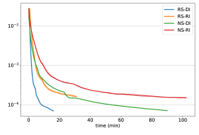
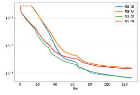
Objective Profiles for Laplace, $n=5{,}000$, $d=4$
relobj
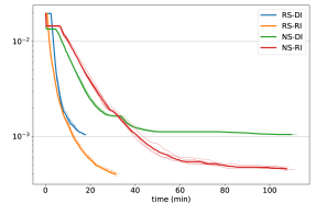
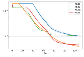
Objective Profiles for Normal, $n=10{,}000$, $d=4$
relobj
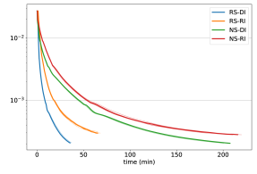
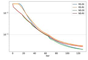
Objective Profiles for Laplace, $n=10{,}000$, $d=4$
relobj

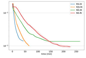
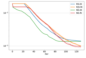
Figure 2: Plots on a log-scale of Relative Objective versus time (mins) [left panel] and number of iterations [right panel]. For each of our four synthetic data sets, we ran five repetitions of each algorithm, so each bold line corresponds to the median of the profiles of the corresponding algorithm, and each thin line corresponds to the profile of one repetition. For the right panel, we show the profiles up to 128 iterations.

Objective Profiles for Normal, $n=5{,}000$, $d=4$
relobj
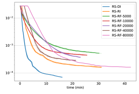
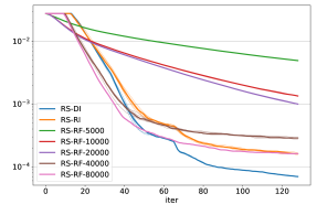
Objective Profiles for Laplace, $n=5{,}000$, $d=4$
relobj
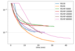
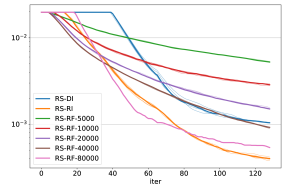
Objective Profiles for Normal, $n=10{,}000$, $d=4$
relobj
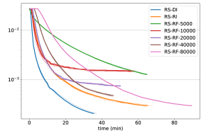
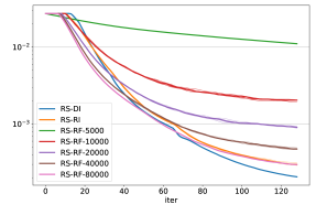
Objective Profiles for Laplace, $n=10{,}000$, $d=4$
relobj

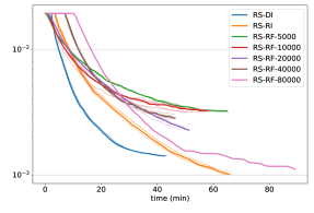
Figure 3: Plots on a log-scale of Relative Objective versus time (mins) [left panel] and number of iterations [right panel].

Appendix A Additional implementational and experimental details

A.1 Initialization: non-convex method

Cule et al., (2010) show that the negative log-density $-\log\hat{p}_{n}(\cdot)$ of the log-concave MLE is a piecewise-affine convex function over its domain $C_{n}$. This allows us to parametrize these functions as $\varphi(\bm{x}):=\max_{j\in[m]}\{\bm{a}_{j}^{\top}\bm{x}+b_{j}\}$ for $x\in C_{n}$, where $\bm{a}_{1},\ldots,\bm{a}_{m}\in\mathbb{R}^{d}$ and $b_{1},\ldots,b_{m}\in\mathbb{R}$. We can then reformulate the problem as $\min_{\bm{a}_{1},\ldots,\bm{a}_{m}\in\mathbb{R}^{d},b_{1},\ldots,b_{m}\in\mathbb{R}}f_{0}(\bm{a},\bm{b})$, with non-convex objective

$$f_{0}(\bm{a},\bm{b}):=\frac{1}{n}\sum_{i=1}^{n}\max_{j\in[m]}\{\bm{a}_{j}^{\top}\bm{x}_{i}+b_{j}\}+\int_{C_{n}}e^{-\max_{j\in[m]}\{\bm{a}_{j}^{\top}\bm{x}+b_{j}\}}~{}d\bm{x}.$$ (28)

To approximate the integral, we use the same simple Riemann grid points mentioned in Section 3.2.1. Subgradients of the objective (28) are straightforward to compute via the chain rule and the subgradient of the maximum function (see, e.g., Bertsekas, (2009)). After standardizing each coordinate of our data to have mean zero and unit variance, which does not affect the final outcome due to the affine equivariance of the log-concave MLE (Dümbgen et al.,, 2011, Remark 2.4), we generate $m=10$ initializing hyperplanes from a standard $(d+1)$-dimensional Gaussian distribution. We then obtain the initializer for our main algorithm by applying a vanilla subgradient method to the objective (28) (Shor,, 1985; Polyak,, 1987) with stepsize $t^{-1/2}$ at the $t$th iteration, terminating when the difference in the objective function at successive iterations drops below $10^{-4}$, or after 100 iterations, whichever is the sooner. This technique is related to the non-convex method for log-concave density estimation proposed by Rathke and Schnörr, (2019), who considered a smoothed version of (28). Our goal here is only to seek a good initializer rather than the global optimum, and we found that the approach described above was effective in this respect, as well as being faster to compute than the method of Rathke and Schnörr, (2019).

A.2 Final polishing step

As mentioned in Section 3.2.1, once our algorithm terminates at $\tilde{\bm{\phi}}_{T}$, say, we evaluate the integral $I(\tilde{\bm{\phi}}_{T})$ in the same way as Cule et al., (2010). Our final output, then is $\bm{\phi}_{T}:=\tilde{\bm{\phi}}_{T}+\log I(\tilde{\bm{\phi}}_{T})\bm{1}$; this final step not only improves the objective function, but also guarantees that $\exp[-\mathrm{cef}[\bm{\phi}_{T}](\cdot)]$ is a log-concave density. This can be shown by following the same arguments as in Steps 2-3 in the proof of Theorem 4.

A.3 Input parameter settings

According to Theorem 1, we should take $u=\frac{D}{2}\sqrt{\frac{B_{1}}{B_{0}}}$. By Table 2, for randomized smoothing, this is approximately $\frac{D}{2}C_{1}\sqrt{n}$, where $C_{1}=\sqrt{\Delta e^{-\phi_{0}}}$. In our experiments for randomized smoothing, we chose $u=Dn^{1/4}/2$, while for Nesterov smoothing, we chose $u=D/2$. According to Theorem 1, $\eta=\sigma M_{T}^{(1)}/D$, where we took $\sigma=10^{-4}$ for RS-RI and RS-DI, and $\sigma=10^{-3}$ for NS-RI and NS-DI. For the competing RS-RF-$m$ method, we present the better of the results from $\sigma\in\{10^{-3},10^{-4}\}$.

Table 5: Examples of increasing grid size ($|\mathcal{S}_{t}|=m_{t}$) schemes to achieve $\tilde{O}(1/T)$ rate (i.e. $M_{T}^{(1/2)}=\tilde{O}(1)$ for deterministic $\mathcal{S}_{t}$ and $M_{T}^{(1)}=\tilde{O}(1)$ for random $\mathcal{S}_{t}$). Here, $C$ and $C_{1}$ are positive constants. For the multi-stage scheme, $a\geq 1$ denotes the current stage number.

Schemes	Grid Sizes	$M_{T}^{(1/2)}=\tilde{O}(1)$	$M_{T}^{(1)}=\tilde{O}(1)$
Exponential	$m_{t}=C\rho^{t}$	$\rho>1$	$\rho>1$
Polynomial	$m_{t}=Ct^{\beta}$	$\beta\geq 2$	$\beta\geq 1$
Multi-stage	$m_{t}=C\rho^{a}$ for	$\rho_{1}^{2}\leq\rho$	$\rho_{1}\leq\rho$
	$t\in\bigl{[}\mathbbm{1}_{\{a\geq 1\}}+C_{1}\rho_{1}^{a-1}\mathbbm{1}_{\{a\geq 2\}},C_{1}\rho_{1}^{a}\bigr{]}$

To illustrate the increasing grid size strategy we take in the experiments, we first present in Table 5 some potential schemes to achieve the $\tilde{O}(1/T)$ error rate on the objective function scale. In our experiments, we used the multi-stage increasing grid size scheme with $C_{1}=8$ and $\rho_{1}=2$. For the random grid (RI), we take $C=5{,}000$ and $\rho=2$. For the deterministic grid (DI), we first choose an axis-aligned grid with $m_{0,t}$ points in each dimension that encloses the convex hull $C_{n}$ of the data. Then $m_{t}$ is the number of these grid points that fall within $C_{n}$. Table 6 provides an illustration of this multi-stage strategy used in the numerical experiments for a Laplace distribution with $n=5{,}000$ and $d=4$. Code for the other settings is available in the github repository LogConcComp.

Table 6: Summary of increasing grid size strategy (illustrated with $n=5{,}000$ observations from a Laplace distribution in four dimensions). We take a four stage grid strategy and 128 iterations in total, with stage lengths shown in second line. For deterministic grids (denoted by DI), we use $m_{0,t}$ to determine the grid size (third line in the table), and the fourth line of the table is the corresponding grid size. For random grids (denoted by RI), the fifth line is the grid size of random sample.

Stage number $a$		1	2	3	4
Stage length		16	16	32	64
DI	$m_{0,t}$	18	22	26	30
DI	$m_{t}$	10,656	23,582	45,969	81,558
RI	$m_{t}$	10,000	20,000	40,000	80,000

A.4 Experimental results on real data sets

We provide additional simulation results on three real data sets:

• Stock returns: The Stock returns real data consist of daily returns of four stocks over $n=10{,}000$ randomly sampled days between 1970 and 2010, normalized so that each dimension has unit variance. The real data are available at https://stooq.com/db/h/.

• Census: The Census real data consist of percentages of the population of different age groups (18-24, 25-44, 45-64 and 65+) for $n=10{,}000$ randomly sampled Census tracts based on the 2015-2019 5-year ACS (American Community Survery), and the data are normalized so that each dimension has unit variance. The data and description are available at https://www.census.gov/topics/research/guidance/planning-databases/2021.html.

• Gas turbine: The Gas turbine real data consist of 4 sensor measures aggregated over one hour from a gas turbine for $n=10{,}000$ hours between 2011 and 2015, normalized so that each dimension has unit variance. The data are available at https://archive.ics.uci.edu/ml/datasets/Gas+Turbine+CO+and+NOx+Emission+Data+Set.

Table 7, Figure 4 and Figure 5 provide simulation results that correspond to those in Table 3, Figure 2 and Figure 3 respectively, but for three three real data sets. The table and figures reveal a qualitatively very similar story to that presented for the simulated data in Section 6: the main conclusion is that our randomized smoothing approaches are significantly more computationally efficient than both the Nesterov smoothing and CSS methods.

Table 7: Comparison of our proposed methods with the CSS solution Cule et al., (2010) and RS-RF Duchi et al., (2012), but on 3 real datasets. Details are given in the caption of Table 3.

Stock returns, $n=10{,}000,d=4$
algo param obj relobj runtime dopt iter tO aO hO CSS 1e-2 6.3395 6.7e-02 315.19 5.4659 1e-3 5.9458 8.7e-04 - 0.5130 1e-4 5.9406 0.0e-00 - 0.0000 RS-DI None 5.9589 3.1e-03 38.47 0.1428 128 7.79M 60.86K 30.22K RS-RI None 5.9778 6.3e-03 59.65 0.2032 128 6.88M 53.75K 32.00K NS-DI None 5.9506 1.7e-03 254.91 0.0792 128 7.79M 60.86K 30.22K NS-RI None 5.9672 4.5e-03 228.82 0.1362 128 6.88M 53.75K 32.00K RS-RF 5000 6.0003 1.0e-02 61.98 0.2015 1024 5.12M 5.00K 5.00K 10000 5.9886 8.1e-03 54.20 0.2354 512 5.12M 10.00K 10.00K 20000 5.9852 7.5e-03 49.16 0.2141 256 5.12M 20.00K 20.00K 40000 5.9940 9.0e-03 46.25 0.3194 128 5.12M 40.00K 40.00K 80000 5.9665 4.4e-03 84.59 0.1055 128 10.24M 80.00K 80.00K
Census, $n=10{,}000,d=4$
algo param obj relobj runtime dopt iter tO aO hO CSS 1e-2 5.4458 9.4e-03 71.36 0.9222 1e-3 5.3953 1.2e-05 812.49 0.0098 1e-4 5.3952 0.0e-00 - 0.0000 RS-DI None 5.3995 8.0e-04 31.97 0.0478 128 6.19M 48.33K 25.79K RS-RI None 5.4003 9.4e-04 63.32 0.0506 128 6.88M 53.75K 32.00K NS-DI None 5.3992 7.3e-04 199.74 0.0453 128 6.19M 48.33K 25.79K NS-RI None 5.3992 7.4e-04 223.34 0.0475 128 6.88M 53.75K 32.00K RS-RF 5000 5.4100 2.7e-03 69.86 0.1047 1024 5.12M 5.00K 5.00K 10000 5.4093 2.6e-03 60.79 0.0796 512 5.12M 10.00K 10.00K 20000 5.4074 2.3e-03 55.89 0.1236 256 5.12M 20.00K 20.00K 40000 5.4059 2.0e-03 49.04 0.0587 128 5.12M 40.00K 40.00K 80000 5.3998 8.6e-04 94.51 0.0477 128 10.24M 80.00K 80.00K
Gas turbine, $n=10{,}000,d=4$
algo param obj relobj runtime dopt iter tO aO hO CSS 1e-2 5.5920 5.7e-03 95.59 0.5908 1e-3 5.5617 2.7e-04 - 0.0994 1e-4 5.5602 0.0e-00 - 0.0000 RS-DI None 5.5693 1.6e-03 34.14 0.0897 128 7.08M 55.28K 25.53K RS-RI None 5.5633 5.7e-04 61.90 0.0493 128 6.88M 53.75K 32.00K NS-DI None 5.5689 1.6e-03 230.47 0.0914 128 7.08M 55.28K 25.53K NS-RI None 5.5622 3.7e-04 224.88 0.0499 128 6.88M 53.75K 32.00K RS-RF 5000 5.5694 1.7e-03 67.28 0.1111 1024 5.12M 5.00K 5.00K 10000 5.5670 1.2e-03 61.22 0.0794 512 5.12M 10.00K 10.00K 20000 5.5673 1.3e-03 53.08 0.0455 256 5.12M 20.00K 20.00K 40000 5.5657 9.9e-04 47.80 0.0547 128 5.12M 40.00K 40.00K 80000 5.5632 5.5e-04 92.44 0.0501 128 10.24M 80.00K 80.00K

Objective Profiles for Stock returns, $n=10{,}000$, $d=4$
relobj
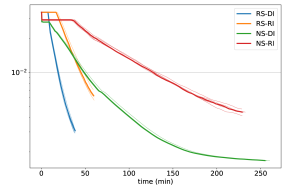
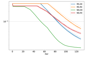
Objective Profiles for Census, $n=10{,}000$, $d=4$
relobj
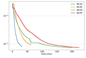
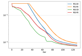
Objective Profiles for Gas turbine, $n=10{,}000$, $d=4$
relobj

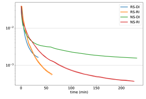
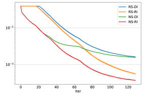
Figure 4: Additional plots on a log-scale of Relative Objective versus time (mins) [left panel] and number of iterations [right panel]. Details are given in the caption of Figure 2.

Objective Profiles for Stock returns, $n=10{,}000$, $d=4$
relobj
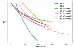
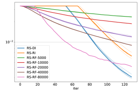
Objective Profiles for Census, $n=10{,}000$, $d=4$
relobj
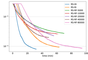
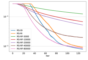
Objective Profiles for Gas turbine, $n=10{,}000$, $d=4$
relobj

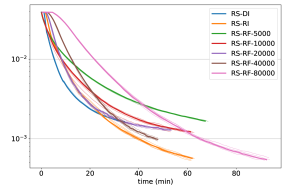
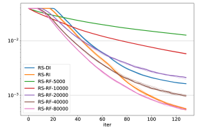
Figure 5: Plots on a log-scale of Relative Objective versus time (mins) [left panel] and number of iterations [right panel].

Appendix B Proofs

B.1 Proofs of Propositions 1 and 2

The proof of Proposition 1 is adapted from the proof of Axelrod et al., (2019, Lemma 2), which in turn is based on Carpenter et al., (2018, Lemma 8). [Proof of Proposition 1] The proof has three parts.

Part 1. We first prove that $\phi^{*}_{i}\in[\phi_{0},\phi^{0}]$ for all $i\in[n]$; or equivalently

$$\begin{aligned} \log\hat{p}_{n}(\bm{x}_{i})&\geq-(n-1)-d(n-1)\log\bigl{(}2n+2nd\log(2nd)\bigr{)}-\log\Delta\\ \log\hat{p}_{n}(\bm{x}_{i})&\leq 1+d\log\bigl{(}2n+2nd\log(2nd)\bigr{)}-\log\Delta\end{aligned}$$ (29)

for all $i\in[n]$. Define

$$M:=\sup_{\bm{x}\in\mathbb{R}^{d}}\hat{p}_{n}(\bm{x})=\max_{i\in[n]}\hat{p}_{n}(\bm{x}_{i})~{}~{}~{}\text{and}~{}~{}R:=\frac{\max_{i\in[n]}\hat{p}_{n}(\bm{x}_{i})}{\min_{i\in[n]}\hat{p}_{n}(\bm{x}_{i})}.$$

We proceed to obtain an upper bound on $R$. To this end, let $\bar{p}_{n}$ denote the uniform density over $C_{n}$. If $\hat{p}_{n}(\bm{x}_{i})=\bar{p}_{n}(\bm{x}_{i})=1/\Delta$ for all $i$, then (29) holds. So we may assume that $\hat{p}_{n}\neq\bar{p}_{n}$, so that $R>1$ and $M>1/\Delta$. For a density $p$ on $\mathbb{R}^{d}$ and for $t\in\mathbb{R}$, let $L_{p}(t):=\{\bm{x}\in\mathbb{R}^{d}:p(\bm{x})\geq t\}$ denote the super-level set of $p$ at height $t$. Since $\hat{p}_{n}$ is supported on $C_{n}$, and since $\hat{p}_{n}(\bm{x})\geq\min_{i\in[n]}\hat{p}_{n}(\bm{x}_{i})=M/R$ for $\bm{x}\in C_{n}$, it follows by Carpenter et al., (2018, Lemma 8) that when $R\geq e$,

$$\Delta=\mathrm{vol}(C_{n})\leq\mathrm{vol}\bigl{(}L_{\hat{p}_{n}}(M/R)\bigr{)}\leq\frac{e\log^{d}R}{M}.$$ (30)

On the other hand, since $\inf_{\bm{x}\in C_{n}}\hat{p}_{n}(\bm{x})=M/R$, we have $(M/R)\cdot\Delta\leq 1$, so for $R<e$, we have $M\leq R/\Delta<e/\Delta$. We deduce that

$$M\leq\frac{e\log_{+}^{d}R}{\Delta},$$ (31)

for all $R>1$, where $\log_{+}(x):=1\vee\log x$. Now, by the optimality of $\hat{p}_{n}$, we have

$$n\log(1/\Delta)\!=\!\sum_{i=1}^{n}\log\bar{p}_{n}(\bm{x}_{i})\!\leq\!\sum_{i=1}^{n}\log\hat{p}_{n}(\bm{x}_{i}) \leq\min_{i\in[n]}\log\hat{p}_{n}(\bm{x}_{i})+(n-1)\max_{i\in[n]}\log\hat{p}_{n}(\bm{x}_{i})$$

$$=\log(M/R)+(n-1)\log M,$$ (32)

so that $R\leq(M\Delta)^{n}$. It follows that when $R\geq e$, we have from (31) and the fact that $\log y\leq y$ for $y>0$ that

$$R=\frac{R^{2}}{R}\leq\frac{e^{2n}\log^{2nd}R}{R}\leq e^{2n}(2nd)^{2nd}.$$ (33)

Since (33) holds trivially when $R<e$, we may combine (33) with (31) to obtain

$$\log M\leq 1+d\log\bigl{(}2n+2nd\log(2nd)\bigr{)}-\log\Delta$$ (34)

Moreover, from (B.1) and (34), we also have

$$\log(M/R) \geq-n\log\Delta-(n-1)\log M$$

$$\geq-(n-1)-d(n-1)\log\bigl{(}2n+2nd\log(2nd)\bigr{)}-\log\Delta,$$

as required.

Part 2. Now we extend the above result to all $\bm{\phi}\in\mathbb{R}^{n}$ such that $I(\bm{\phi})=1$ and $f(\bm{\phi})\leq f(\bar{\bm{\phi}})$, where $\bar{\bm{\phi}}$ is defined just after Proposition 1. The key observation here is that the proof of Part 1 applies to any density with log-likelihood at least that of the uniform distribution over $C_{n}$. In particular, for any $\bm{\phi}$ satisfying these conditions, the density $p\in\mathcal{F}_{d}$ given by $p(\bm{x})=\exp\{-\mathrm{cef}[\bm{\phi}](\bm{x})\}$ has log-likelihood at least that of the uniform distribution over $C_{n}$, so

$$-\phi^{0}\leq\min_{i\in[n]}\log p(\bm{x}_{i})\leq\sup_{\bm{x}\in\mathbb{R}^{d}}\log p(\bm{x})\leq-\phi_{0},$$

as required.

Part 3. We now consider the case for a general $\bm{\phi}\in\mathbb{R}^{n}$ with $f(\bm{\phi})\leq f(\bar{\bm{\phi}})$. Let $\tilde{\bm{\phi}}:=\bm{\phi}+\log I(\bm{\phi})\bm{1}$, so that $I(\tilde{\bm{\phi}})=1$ and $\mathrm{cef}[\tilde{\bm{\phi}}](\cdot)=\mathrm{cef}[\bm{\phi}](\cdot)+\log(I(\bm{\phi}))$. Furthermore,

$$f(\tilde{\bm{\phi}})=\frac{1}{n}\bm{1}^{\top}\bm{\phi}+\log I(\bm{\phi})+1\leq\frac{1}{n}\bm{1}^{\top}\bm{\phi}+I(\bm{\phi})=f(\bm{\phi})\leq f(\bar{\bm{\phi}}).$$

The result therefore follows by Part 2.

[Proof of Proposition 2] Recall our notation from Section 2 that $\bm{\alpha}^{*}[\bm{\phi}](\bm{x})\in A[\bm{\phi}](\bm{x})$ denotes a solution to ($Q_{0}$) at $\bm{x}\in C_{n}$. Recall further from (9) that any subgradient $\bm{g}(\bm{\phi})$ of $f$ at $\bm{\phi}$ is of the form

$$\bm{g}(\bm{\phi})=\frac{1}{n}\bm{1}-\bm{\gamma},$$

where $\bm{\gamma}:=\Delta\mathbb{E}\bigl{[}\bm{\alpha}^{*}[\bm{\phi}](\bm{\xi})\exp\{-\mathrm{cef}[\bm{\phi}](\bm{\xi})\}\bigr{]}$ and $\bm{\xi}$ is uniformly distributed on $C_{n}$. Since $\bm{\alpha}^{*}$ lies in the simplex $\{\bm{\alpha}\in\mathbb{R}^{n}:\bm{\alpha}\geq 0,\bm{1}^{\top}\bm{\alpha}=1\},$ we have $\bm{\gamma}\geq 0$ and

$$\bm{1}^{\top}\bm{\gamma}=\Delta\mathbb{E}[\bm{1}^{\top}\alpha^{*}[\bm{\phi}](\bm{\xi})\exp\{-\mathrm{cef}[\bm{\phi}](\bm{\xi})\}]=\Delta\mathbb{E}[\exp\{-\mathrm{cef}[\bm{\phi}](\bm{\xi})\}]=I(\bm{\phi}).$$

In particular, $\left\lVert\bm{\gamma}\right\rVert_{1}=I(\bm{\phi})$, so

$$\|\bm{g}(\bm{\phi})\|^{2}=\frac{1}{n}-\frac{2}{n}\bm{1}^{\top}\bm{\gamma}+\|\bm{\gamma}\|^{2}\leq\frac{1}{n}-\frac{2}{n}I(\bm{\phi})+I(\bm{\phi})^{2}.$$

If $I(\bm{\phi})\leq 1/2$, then $\left\lVert\bm{g}(\bm{\phi})\right\rVert^{2}\leq 1/4+1/n$; if $I(\phi)>1/2$, then $\left\lVert\bm{g}(\bm{\phi})\right\rVert^{2}\leq I(\bm{\phi})^{2}$. Therefore, $\left\lVert\bm{g}(\bm{\phi})\right\rVert^{2}\leq\max\bigl{\{}1/4+1/n,I(\bm{\phi})^{2}\bigr{\}}$.

B.2 Proofs of Proposition 3 and Proposition 4

The proof of Proposition 3 is based on the following properties of the quadratic program $q_{u}[\bm{\phi}](\bm{x})$ defined in ($Q_{u}$), as well as its unique optimizer $\bm{\alpha}_{u}^{*}[\bm{\phi}](\bm{x})$:

Proposition 5.

For $\bm{\phi}\in\bm{\Phi}$ and $\bm{x}\in C_{n}$, we have

(a) $\|\bm{\alpha}_{u}^{*}[\bm{\phi}](\bm{x})\|\leq 1$ for any $\bm{x}\in C_{n}$ and $\bm{\phi}\in\bm{\Phi}$;

(b) $q_{u^{\prime}}[\bm{\phi}](\bm{x})+(u^{\prime}-u)/2\leq q_{u}[\bm{\phi}](\bm{x})\leq q_{u^{\prime}}[\bm{\phi}](\bm{x})$ for $u^{\prime}\in[0,u]$;

(c) $\phi_{0}-\frac{u}{2}\leq q_{u}[\bm{\phi}](\bm{x})\leq\phi^{0}$ for all $u\geq 0$, $\bm{\phi}\in\bm{\Phi}$ and $\bm{x}\in C_{n}$;

(d) $\|\bm{\alpha}_{u}^{*}[\tilde{\bm{\phi}}](\bm{x})-\bm{\alpha}_{u}^{*}[\bm{\phi}](\bm{x})\|\leq({1}/{u})\|\tilde{\bm{\phi}}-\bm{\phi}\|$ for any $u>0$, $\bm{\phi},\tilde{\bm{\phi}}\in\bm{\bm{\Phi}}$, and any $\bm{x}\in C_{n}$.

[Proof.]The proof exploits ideas from Nesterov, (2005). For (a), observe that $\bm{\alpha}_{u}^{*}[\bm{\phi}](\bm{x})\in E(\bm{x})\subseteq\{\bm{\alpha}\in\mathbb{R}^{n}:\bm{1}_{n}^{\top}\bm{\alpha}=1,\bm{\alpha}\geq 0\bigr{\}}$, and this simplex is the convex hull of $n+1$ points that all lie in the closed unit Euclidean ball in $\mathbb{R}^{n}$.

The lower bound in (b) follows immediately from the definition of the quadratic program in ($Q_{u}$). For the upper bound, for $u^{\prime}\in[0,u]$, we have

$$~{}q_{u}[\bm{\phi}](\bm{x})-q_{u^{\prime}}[\bm{\phi}](\bm{x})$$

$$=\bm{\alpha}^{*}_{u}[\bm{\phi}](\bm{x})^{\top}\bm{\phi}+\frac{u}{2}\bigl{\|}\bm{\alpha}_{u}^{*}[\bm{\phi}](\bm{x})-\bm{\alpha}_{0}\bigr{\|}^{2}-\bm{\alpha}^{*}_{u^{\prime}}[\bm{\phi}](\bm{x})^{\top}\bm{\phi}-\frac{u^{\prime}}{2}\bigl{\|}\bm{\alpha}_{u^{\prime}}^{*}[\bm{\phi}](\bm{x})-\bm{\alpha}_{0}\bigr{\|}^{2}+\frac{u^{\prime}-u}{2}$$

$$\leq\frac{u-u^{\prime}}{2}\biggl{(}\bigl{\|}\bm{\alpha}_{u^{\prime}}^{*}[\bm{\phi}](\bm{x})-\bm{\alpha}_{0}\bigr{\|}^{2}-1\biggr{)}\leq\frac{u-u^{\prime}}{2}\biggl{(}1-\frac{2}{n}+\frac{1}{n}-1\biggr{)}\leq 0.$$

(c) For all $u\geq 0$, $\bm{\phi}\in\bm{\Phi}$ and $\bm{x}\in C_{n}$, we have

$$q_{u}[\bm{\phi}](\bm{x})=\inf_{\bm{\alpha}\in E(\bm{x})}\biggl{(}\bm{\alpha}^{\top}\bm{\phi}+\frac{u}{2}\|\bm{\alpha}-\bm{\alpha}_{0}\|^{2}-\frac{u}{2}\biggr{)} \geq\inf_{\bm{\alpha}\in E(\bm{x})}\bm{\alpha}^{\top}\bm{\phi}-\frac{u}{2}$$

$$\geq\phi_{0}\inf_{\bm{\alpha}\in E(\bm{x})}\bm{\alpha}^{\top}\bm{1}_{n}-\frac{u}{2}=\phi_{0}-\frac{u}{2}.$$

Similarly,

$$q_{u}[\bm{\phi}](\bm{x})\leq\phi^{0}\sup_{\bm{\alpha}\in E(\bm{x})}\bm{\alpha}^{\top}\bm{1}_{n}+\frac{u}{2}\sup_{\bm{\alpha}\in E(\bm{x})}\|\bm{\alpha}-\bm{\alpha}_{0}\|^{2}-\frac{u}{2}\leq\phi^{0}.$$

(d) Observe that

$$\bm{\alpha}_{u}^{*}[\bm{\phi}](\bm{x})=\operatorname*{argmin}_{\bm{\alpha}\in E(\bm{x})}~{}\biggl{(}\bm{\alpha}^{\top}\bm{\phi}+\frac{u}{2}\|\bm{\alpha}-\bm{\alpha}_{0}\|^{2}\biggr{)}=\operatorname*{argmin}_{\bm{\alpha}\in E(\bm{x})}~{}\biggl{\|}\bm{\alpha}-\biggl{(}\bm{\alpha}_{0}-\frac{\bm{\phi}}{u}\biggr{)}\biggr{\|}^{2},$$

so $\bm{\alpha}_{u}^{*}[\bm{\phi}](\bm{x})$ is the Euclidean projection of $\bm{\alpha}_{0}-({\bm{\phi}}/{u})$ onto $E(\bm{x})$. Since this projection is an $\ell_{2}$-contraction, we deduce that

$$\bigl{\|}\bm{\alpha}_{u}^{*}[\tilde{\bm{\phi}}](\bm{x})-\bm{\alpha}_{u}^{*}[\bm{\phi}](\bm{x})\bigr{\|}\leq\biggl{\|}\bm{\alpha}_{0}-\frac{\tilde{\bm{\phi}}}{u}-\biggl{(}\bm{\alpha}_{0}-\frac{\bm{\phi}}{u}\biggr{)}\biggr{\|}=\frac{1}{u}\|\tilde{\bm{\phi}}-\bm{\phi}\|,$$

as required.

[Proof of Proposition 3] (a) For $u\geq 0$ and $\bm{\phi}\in\bm{\Phi}$, let

$$\tilde{I}_{u}(\bm{\phi}):=\int_{C_{n}}e^{-q_{u}[\bm{\phi}](\bm{x})}\,d\bm{x}=\Delta\mathbb{E}(e^{-q_{u}[\bm{\phi}](\bm{\xi})}),$$

where $\bm{\xi}$ is uniformly distributed on $C_{n}$, so that $\tilde{I}_{0}(\bm{\phi})=I(\bm{\phi})$. By definition of $\tilde{f}_{u}$, we have for $u^{\prime}\in[0,u]$ that

$$\tilde{f}_{u}(\bm{\phi})-\tilde{f}_{u^{\prime}}(\bm{\phi})=\tilde{I}_{u}(\bm{\phi})-\tilde{I}_{u^{\prime}}(\bm{\phi})=\Delta\mathbb{E}\bigl{(}e^{-q_{u}[\bm{\phi}](\bm{\xi})}-e^{-q_{u^{\prime}}[\bm{\phi}](\bm{\xi})}\bigr{)}\geq 0,$$ (35)

where the inequality follows from Proposition 5(b). Hence, for every $u\geq 0$ and $\bm{\phi}\in\bm{\Phi}$,

$$\tilde{I}_{u}(\bm{\phi})\leq e^{u/2}\tilde{I}_{0}(\bm{\phi})=e^{u/2}I(\bm{\phi}).$$ (36)

Now, from (35), Proposition 5(b) and (36), we deduce that

$$\tilde{f}_{u}(\bm{\phi})-\tilde{f}_{u^{\prime}}(\bm{\phi})\leq\bigl{(}e^{(u-u^{\prime})/2}-1\bigr{)}\tilde{I}_{u^{\prime}}(\bm{\phi})\leq\frac{u-u^{\prime}}{2}e^{u^{\prime}/2}I(\bm{\phi}),$$

as required.

(b) For each $\bm{x}\in C_{n}$, the function $\bm{\phi}\mapsto q_{u}[\bm{\phi}](\bm{x})$ is the infimum of a set of affine functions of $\bm{\phi}$, so it is concave. Moreover, $y\mapsto e^{-y}$ is a decreasing convex function, so $\bm{\phi}\mapsto e^{-q_{u}[\bm{\phi}](\bm{x})}$ is convex, and it follows that $\bm{\phi}\mapsto(1/n)\bm{1}^{\top}\bm{\phi}+\Delta\mathbb{E}(e^{-q_{u}[\bm{\phi}](\bm{\xi})})=\tilde{f}_{u}(\bm{\phi})$ is convex. Similarly to the proof of Proposition 2, any subgradient $\tilde{\bm{g}}_{u}(\phi)$ of $\tilde{f}_{u}$ at $\bm{\phi}$ satisfies

$$\left\lVert\tilde{\bm{g}}_{u}(\bm{\phi})\right\rVert^{2}\leq\max\biggl{\{}\frac{1}{4}+\frac{1}{n},\tilde{I}_{u}(\bm{\phi})^{2}\biggr{\}}\leq\max\biggl{\{}\frac{1}{4}+\frac{1}{n},\Delta^{2}e^{-2\phi_{0}+u}\biggr{\}}.$$ (37)

But $\bm{\phi}^{*}\in\bm{\Phi}$, so $\Delta^{2}e^{-2\phi_{0}+u}\geq(\Delta e^{-\phi_{0}})^{2}\geq I(\bm{\phi}^{*})^{2}=1\geq 1/4+1/n$. Hence, $\tilde{f}_{u}$ is $e^{-\phi_{0}+u/2}$-Lipschitz.

(c) To establish the Lipschitz property of $\nabla_{\bm{\phi}}\tilde{f}_{u}$, for any $\bm{x}\in C_{n}$, any $\bm{\phi},\tilde{\bm{\phi}}\in\bm{\Phi}$, and $t\in[0,1]$, we define

$$\eta(t):=e^{-q_{u}[\bm{\phi}+t(\tilde{\bm{\phi}}-\bm{\phi})](\bm{x})}.$$

Then

$$\eta^{\prime}(t)=-e^{-q_{u}[\bm{\phi}+t(\tilde{\bm{\phi}}-\bm{\phi})](\bm{x})}(\tilde{\bm{\phi}}-\bm{\phi})^{\top}\bm{\alpha}_{u}^{*}[\bm{\phi}+t(\tilde{\bm{\phi}}-\bm{\phi})](\bm{x}).$$

By the mean value theorem there exists $t_{0}\in[0,1]$ such that

$$\bigl{|}e^{-q_{u}[\tilde{\bm{\phi}}](\bm{x})}-e^{-q_{u}[\bm{\phi}](\bm{x})}\bigr{|}=|\eta(1)\!-\!\eta(0)|=|\eta^{\prime}(t_{0})|$$

$$\leq e^{-q_{u}[\bm{\phi}+t_{0}(\tilde{\bm{\phi}}-\bm{\phi})](\bm{x})}\|\tilde{\bm{\phi}}-\bm{\phi}\|\bigl{\|}\bm{\alpha}_{u}^{*}[\bm{\phi}+t_{0}(\tilde{\bm{\phi}}-\bm{\phi})](\bm{x})\bigr{\|}$$

$$\leq e^{-\phi_{0}+u/2}\|\tilde{\bm{\phi}}-\bm{\phi}\|,$$ (38)

where the final bound follows from Proposition 5(a) and (c). Now, for any $\bm{x}\in C_{n}$, we have by (B.2) as well as Proposition 5(a), (c) and (d) that

$$\bigl{\|}e^{-q_{u}[\tilde{\bm{\phi}}](\bm{x})}\bm{\alpha}_{u}^{*}[\tilde{\bm{\phi}}](\bm{x})-e^{-q_{u}[\bm{\phi}](\bm{x})}\bm{\alpha}_{u}^{*}[\bm{\phi}](\bm{x})\bigr{\|}$$

$$=\bigl{\|}\bigl{(}e^{-q_{u}[\tilde{\bm{\phi}}](\bm{x})}-e^{-q_{u}[\bm{\phi}](\bm{x})}\bigr{)}\bm{\alpha}_{u}^{*}[\tilde{\bm{\phi}}](\bm{x})+e^{-q_{u}[\bm{\phi}](\bm{x})}\bigl{(}\bm{\alpha}_{u}^{*}[\tilde{\bm{\phi}}](\bm{x})-\bm{\alpha}_{u}^{*}[\bm{\phi}](\bm{x})\bigr{)}\bigr{\|}$$

$$\leq e^{-\phi_{0}+u/2}\|\tilde{\bm{\phi}}-\bm{\phi}\|+e^{+}u/2{-\phi_{0}}\frac{1}{u}\|\tilde{\bm{\phi}}-\bm{\phi}\|=e^{-\phi_{0}+u/2}(1+u^{-1})\|\tilde{\bm{\phi}}-\bm{\phi}\|.$$

It follows that for any $\bm{\phi},\tilde{\bm{\phi}}\in\bm{\Phi}$, we have

$$\bigl{\|}\nabla_{\tilde{\bm{\phi}}}\tilde{f}_{u}(\tilde{\bm{\phi}})-\nabla_{\bm{\phi}}\tilde{f}_{u}(\bm{\phi})\bigr{\|}\leq\Delta\mathbb{E}\bigl{\|}e^{-q_{u}[\tilde{\bm{\phi}}](\bm{\xi})}\bm{\alpha}_{u}^{*}[\tilde{\bm{\phi}}](\bm{\xi}) -e^{-q_{u}[\bm{\phi}](\bm{\xi})}\bm{\alpha}_{u}^{*}[\bm{\phi}](\bm{\xi})\bigr{\|}$$

$$\leq\Delta e^{-\phi_{0}+u/2}(1+u^{-1})\|\tilde{\bm{\phi}}-\bm{\phi}\|,$$

as required.

(d) For $u\geq 0$ and $\bm{\phi}\in\bm{\Phi}$, it follows from Proposition 5(a) and (c) that

$$\mathbb{E}\bigl{(}\|{\tilde{\bm{G}}_{u}(\bm{\phi},\bm{\xi})-\nabla\tilde{f}_{u}(\bm{\phi})}\|^{2}\bigr{)} =\mathbb{E}\bigl{\|}\Delta e^{-q_{u}[\bm{\phi}](\bm{\xi})}\bm{\alpha}_{u}^{*}[\bm{\phi}](\bm{\xi})-\Delta\mathbb{E}\bigl{(}e^{-q_{u}[\bm{\phi}](\bm{\xi})}\bm{\alpha}_{u}^{*}[\bm{\phi}](\bm{\xi})\bigr{)}\bigr{\|}^{2}$$

$$\leq\Delta^{2}\mathbb{E}\bigl{\|}e^{-q_{u}[\bm{\phi}](\bm{\xi})}\bm{\alpha}_{u}^{*}[\bm{\phi}](\bm{\xi})\bigr{\|}^{2}\leq(\Delta e^{-\phi_{0}+u/2})^{2},$$

as required.

Proposition 6.

If $\bm{z}$ is uniformly distributed on the unit $\ell_{2}$-ball in $\mathbb{R}^{n}$, then $\mathbb{E}(\left\lVert\bm{z}\right\rVert_{\infty})\leq\sqrt{\tfrac{2\log n}{n+1}}$.

[Proof.]By Xu and Samworth, (2021, Proposition 3), we have that $\bm{z}\overset{d}{=}U^{1/n}\bm{z}^{\prime}$, where $U\sim\mathcal{U}[0,1]$, where $\bm{z}^{\prime}$ is uniformly distributed on the unit sphere in $\mathbb{R}^{n}$, and where $U$ and $\bm{z}^{\prime}$ are independent. Thus,

$$\mathbb{E}(\left\lVert\bm{z}\right\rVert_{\infty})=\mathbb{E}(U^{1/n})\mathbb{E}(\left\lVert\bm{z}^{\prime}\right\rVert_{\infty})=\frac{n}{n+1}\mathbb{E}(\left\lVert\bm{z}^{\prime}\right\rVert_{\infty}).$$ (39)

Moreover, if $\bm{\zeta}\sim\mathcal{N}(0,I_{n})$, then $\left\lVert\bm{\zeta}\right\rVert$ and $\bm{\zeta}/\left\lVert\bm{\zeta}\right\rVert$ are independent, and $\bm{z}^{\prime}\overset{d}{=}\bm{\zeta}/\left\lVert\bm{\zeta}\right\rVert$. It follows that

$$\mathbb{E}(\left\lVert\bm{z}^{\prime}\right\rVert_{\infty})\!=\!\mathbb{E}\biggl{(}\frac{\|\bm{\zeta}\|_{\infty}}{\|\bm{\zeta}\|}\biggr{)}\cdot\frac{\mathbb{E}(\|\bm{\zeta}\|)}{\mathbb{E}(\|\bm{\zeta}\|)}\!=\!\frac{\mathbb{E}(\|\bm{\zeta}\|_{\infty})}{\mathbb{E}(\|\bm{\zeta}\|)}=\frac{\sqrt{2\log n}\cdot\Gamma(n/2)}{2^{1/2}\Gamma\bigl{(}(n+1)/2\bigr{)}}\leq\frac{1}{n}\sqrt{2(n+1)\log n},$$ (40)

where the final bound follows from bounds on the gamma function, e.g. (Dümbgen et al.,, 2021, Lemma 12). The result follows from (39) and (40).

[Proof of Proposition 4] (a) By Jensen’s inequality,

$$\bar{f}_{u}(\bm{\phi})=\mathbb{E}f(\bm{\phi}+u\bm{z})\geq f(\bm{\phi}).$$ (41)

For the upper bound, let $\bm{v}\in\mathbb{R}^{n}$ have $\|\bm{v}\|\leq 1$ and, for some $\bm{\phi}\in\bm{\Phi}$, let $\bar{\bm{\phi}}:=\bm{\phi}+u\bm{v}$. For any $\bm{\alpha}\in E(\bm{x})$, we have

$$|\bm{\alpha}^{\top}\bar{\bm{\phi}}-\bm{\alpha}^{\top}\bm{\phi}|=u|\bm{\alpha}^{\top}\bm{v}|\leq u\left\lVert\bm{\alpha}\right\rVert_{1}\left\lVert\bm{v}\right\rVert_{\infty}\leq u.$$

Therefore, for any $\bm{x}\in C_{n}$, we have $\mathrm{cef}[\bar{\bm{\phi}}](\bm{x})\geq\mathrm{cef}[\bm{\phi}](\bm{x})-u.$ Hence

$$I(\bar{\bm{\phi}})=\Delta\mathbb{E}[\exp\{-\mathrm{cef}[\bar{\bm{\phi}}](\bm{\xi})\}]\leq e^{u}\Delta\mathbb{E}[\exp\{-\mathrm{cef}[\bm{\phi}](\bm{\xi})\}]=e^{u}I(\bm{\phi}).$$ (42)

Recall that all subgradients of $I$ at $\tilde{\bm{\phi}}\in\mathbb{R}^{n}$ are of the form $-\bm{\gamma}(\tilde{\bm{\phi}})$, where

$$\bm{\gamma}(\tilde{\bm{\phi}})=\Delta\mathbb{E}\bigl{(}\bm{\alpha}\exp\{-\mathrm{cef}[\tilde{\bm{\phi}}](\bm{\xi})\}\bigr{)}$$

for some $\bm{\alpha}\in A[\tilde{\bm{\phi}}](\bm{x})$. Moreover, as we saw in the proof of Proposition 2, $\|\bm{\gamma}(\tilde{\bm{\phi}})\|_{1}=I(\tilde{\bm{\phi}})$. We deduce from Rockafellar, (1997, Theorem 24.7) that

$$\bar{f}_{u}(\bm{\phi})-f(\bm{\phi})=\mathbb{E}\bigl{(}I(\bm{\phi}+u\bm{z})-I(\bm{\phi})\bigr{)} \leq u\sup_{\bm{\phi}\in\bm{\Phi},\|\bm{v}\|\leq 1}I(\bm{\phi}+u\bm{v})\mathbb{E}\bigl{(}\|\bm{z}\|_{\infty}\bigr{)}$$

$$\leq I(\bm{\phi})ue^{u}\mathbb{E}\bigl{(}\left\lVert\bm{z}\right\rVert_{\infty}\bigr{)}\leq I(\bm{\phi})ue^{u}\sqrt{\frac{2\log n}{n+1}},$$

where the final inequality uses Proposition 6.

(b) By the convexity of $f$, we have

$$\bar{f}_{u^{\prime}}(\bm{\phi})=\mathbb{E}\bigl{(}f(\bm{\phi}+u^{\prime}\bm{z})\bigr{)}\leq\frac{u^{\prime}}{u}\bar{f}_{u}(\bm{\phi})+\biggl{(}1-\frac{u^{\prime}}{u}\biggr{)}f(\bm{\phi})\leq\bar{f}_{u}(\bm{\phi}),$$

where the last inequality uses property (a).

(c) For each $\bm{v}\in\mathbb{R}^{n}$ with $\|\bm{v}\|=1$, the map $\bm{\phi}\mapsto f(\bm{\phi}+u\bm{v})$ is convex, so $\bm{\phi}\mapsto\mathbb{E}\bigl{(}f(\bm{\phi}+u\bm{z})\bigr{)}=\bar{f}_{u}(\bm{\phi})$ is convex. The proof of the Lipschitz property is very similar to that of Proposition 3(b) and is omitted for brevity.

(d) As in the proof of (a), for any $\bm{v}\in\mathbb{R}^{n}$ with $\|\bm{v}\|\leq 1$, $\bm{x}\in C_{n}$ and $\bm{\alpha}\in A[\bm{\phi}+u\bm{v}](\bm{x})$, we have

$$\bigl{\|}\bm{\alpha}e^{-\mathrm{cef}[\bm{\phi}+u\bm{v}](\bm{x})}\bigr{\|}\leq e^{-\phi_{0}+u}.$$

Since $\nabla_{\bm{\phi}}\bar{f}_{u}(\bm{\phi})=n^{-1}\bm{1}-\Delta\mathbb{E}\bigl{(}\bm{\alpha}^{*}[\bm{\phi}+u\bm{z}](\bm{\xi})e^{-\mathrm{cef}[\bm{\phi}+u\bm{z}](\bm{\xi})}\bigr{)}$, where $\bm{\alpha}^{*}[\bm{\phi}+u\bm{v}](\bm{x})\in A[\bm{\phi}+u\bm{v}](\bm{x})$, we have by Yousefian et al., (2012, Lemma 8) that $\nabla_{\bm{\phi}}\bar{f}_{u}$ is $\Delta e^{-\phi_{0}+u}n^{1/2}/u$-Lipschitz.

(e) The proof is very similar to the proof of Proposition 3(d) and is omitted for brevity.

B.3 Proofs of Theorem 1 and Theorem 2

We will make use of the following lemma:

Lemma 1 (Lemma 4.2 of Duchi et al., (2012)).

Let $\bigl{(}\ell_{u_{t}}(\bm{\phi})\bigr{)}_{t}$ be a smoothing sequence such that $\bm{\phi}\mapsto\ell_{u_{t}}(\bm{\phi})$ has $L_{t}$-Lipschitz gradient. Assume that $\ell_{u_{t}}(\bm{\phi})\leq\ell_{u_{t-1}}(\bm{\phi})$ for $\bm{\phi}\in\bm{\Phi}$. Let $(\bm{\phi}_{t}^{(x)})_{t=0}^{T},(\bm{\phi}^{(y)}_{t})_{t=0}^{T},(\bm{\phi}^{(z)}_{t})_{t=0}^{T}$ be the sequences generated by Algorithm 1. Let $\bm{g}_{t}$ denote an approximation of $\nabla\ell_{u_{t}}(\bm{\phi}_{t}^{(y)})$ with error $\bm{e}_{t}=\bm{g}_{t}-\nabla\ell_{u_{t}}(\bm{\phi}_{t}^{(y)})$. Then for any $\bm{\phi}\in\bm{\Phi}$ and $t\in\mathbb{N}$, we have

$$\frac{1}{\theta_{t}^{2}}\ell_{u_{t}}(\bm{\phi}^{(x)}_{t+1})\leq\sum_{\tau=0}^{t}\frac{1}{\theta_{\tau}}\ell_{u_{\tau}}(\bm{\phi}) +\frac{1}{2}\biggl{(}L_{t+1}+\frac{\eta_{t+1}}{\theta_{t+1}}\biggr{)}\left\lVert\bm{\phi}-\bm{\phi}_{0}\right\rVert^{2}$$

$$+\sum_{\tau=0}^{t}\frac{\left\lVert\bm{e}_{\tau}\right\rVert^{2}}{2\theta_{\tau}\eta_{\tau}}+\sum_{\tau=0}^{t}\frac{1}{\theta_{\tau}}\langle\bm{e}_{\tau},\bm{\phi}-\bm{\phi}^{(z)}_{\tau}\rangle.$$

Recall the definition of the diameter $D$ of $\bm{\Phi}$ given just before Theorem 1.

Corollary 2.

Fix $u,\eta>0$, and assume that Assumption 1 holds with $r\geq u$. Suppose in Algorithm 1 that $u_{t}=\theta_{t}u$, $L_{t}={B_{1}}/{u_{t}}$ and $\eta_{t}=\eta$. Let $(\bm{\phi}_{t}^{(x)})_{t=0}^{T},(\bm{\phi}^{(y)}_{t})_{t=0}^{T},(\bm{\phi}^{(z)}_{t})_{t=0}^{T}$ be the sequences generated by Algorithm 1 and let $\bm{e}_{t}=\bm{g}_{t}-\nabla\ell_{u_{t}}(\bm{\phi}_{t}^{(y)})$. Then for any $\bm{\phi}\in\bm{\Phi}$, we have

$$f(\bm{\phi}_{T}^{(x)})-f(\bm{\phi})\leq\frac{B_{1}D^{2}}{Tu}+\frac{\eta D^{2}}{T}+\frac{1}{T\eta}\sum_{t=0}^{T-1}\left\lVert\bm{e}_{t}\right\rVert^{2}+\theta_{T-1}^{2}\sum_{t=0}^{T-1}\frac{1}{\theta_{t}}\langle\bm{e}_{t},\bm{\phi}\!-\!\bm{\phi}_{t}^{(z)}\rangle+\frac{4B_{0}I(\bm{\phi})u}{T}.$$

[Proof.]By induction, we have that $\theta_{t}\leq{2}/{(t+2)}$ and $\sum_{\tau=0}^{t}{1}/{\theta_{\tau}}={1}/{\theta_{t}^{2}}$ for all $t=0,1,\ldots,T$ Tseng, (2008); Duchi et al., (2012). Using Assumption 1, we have

$$\frac{1}{\theta_{T-1}^{2}}\bigl{(}f(\bm{\phi}_{T}^{(x)})-f(\bm{\phi})\bigr{)} \leq\frac{1}{\theta_{T-1}^{2}}\ell_{u_{T-1}}(\bm{\phi}^{(x)}_{T})-\sum_{t=0}^{T-1}\frac{1}{\theta_{t}}\bigl{(}\ell_{u_{t}}(\bm{\phi})-B_{0}u_{t}\bigr{)}$$

$$=\frac{1}{\theta_{T-1}^{2}}\ell_{u_{T-1}}(\bm{\phi}_{T}^{(x)})-\sum_{t=0}^{T-1}\frac{1}{\theta_{t}}\ell_{u_{t}}(\bm{\phi})+TB_{0}I(\bm{\phi})u.$$

Hence, by Lemma 1,

$$f(\bm{\phi}_{T}^{(x)}) -f(\bm{\phi})$$

$$\leq ~{}\frac{\theta_{T-1}^{2}}{2}\left\lVert\bm{\phi}-\bm{\phi}_{0}\right\rVert^{2}\biggl{(}L_{T}+\frac{\eta_{T}}{\theta_{T}}\biggr{)}+\sum_{t=0}^{T-1}\frac{\theta_{T-1}^{2}}{2\theta_{t}\eta_{t}}\left\lVert\bm{e}_{t}\right\rVert^{2}$$

$$\hskip 128.0374pt+\theta_{T-1}^{2}\sum_{t=0}^{T-1}\frac{1}{\theta_{t}}\langle\bm{e}_{t},\bm{\phi}-\bm{\phi}^{(z)}_{t}\rangle+\theta_{T-1}^{2}TB_{0}I(\bm{\phi})u$$

$$\leq ~{}\frac{B_{1}D^{2}\theta_{T-1}^{2}}{2u\theta_{T}}+\frac{\eta_{T}\theta_{T-1}^{2}D^{2}}{2\theta_{T}}+\sum_{t=0}^{T-1}\frac{\theta_{T-1}^{2}}{2\theta_{t}\eta_{t}}\left\lVert\bm{e}_{t}\right\rVert^{2}$$

$$\hskip 128.0374pt+\theta_{T-1}^{2}\sum_{t=0}^{T-1}\frac{1}{\theta_{t}}\langle\bm{e}_{t},\bm{\phi}-\bm{\phi}^{(z)}_{t}\rangle+\theta_{T-1}^{2}TB_{0}I(\bm{\phi})u$$

$$\leq ~{}\frac{B_{1}D^{2}}{Tu}+\frac{\eta_{T}D^{2}}{T}+\frac{1}{T}\sum_{t=0}^{T-1}\frac{1}{\eta_{t}}\left\lVert\bm{e}_{t}\right\rVert^{2}+\theta_{T-1}^{2}\sum_{t=0}^{T-1}\frac{1}{\theta_{t}}\langle\bm{e}_{t},\bm{\phi}-\bm{\phi}^{(z)}_{t}\rangle+\frac{4B_{0}I(\bm{\phi})u}{T},$$

where we have used the facts that $\theta_{T-1}^{2}/\theta_{T}=\theta_{T}/(1-\theta_{T})\leq 2/T$ and $\theta_{T-1}^{2}/\theta_{t}\leq\theta_{T-1}\leq 2/T$ for $t\in\{0,1,\ldots,T-1\}$ and $\theta_{T-1}^{2}\leq 4/T^{2}$.

[Proof of Theorem 1] According to Corollary 2, it suffices to bound $\theta_{T-1}^{2}\sum_{t=0}^{T-1}\frac{1}{\theta_{t}}\mathbb{E}\bigl{(}\langle\bm{e}_{t},\bm{\phi}-\bm{\phi}^{(z)}_{t}\rangle\bigr{)}$ and $\sum_{t=0}^{T-1}\mathbb{E}\bigl{(}\left\lVert\bm{e}_{t}\right\rVert^{2}\bigr{)}$. To this end, we have by Assumption 2 that

$$\mathbb{E}\bigl{(}\langle\bm{e}_{t},\bm{\phi}-\bm{\phi}^{(z)}_{t}\rangle\bigr{)} =\mathbb{E}\bigl{(}\mathbb{E}(\langle\bm{e}_{t},\bm{\phi}-\bm{\phi}^{(z)}_{t}\rangle\bigm{|}\mathcal{F}_{t-1})\bigr{)}\leq\mathbb{E}\bigl{(}\mathbb{E}(\|\bm{e}_{t}\|\|\bm{\phi}-\bm{\phi}^{(z)}_{t}\|\mid\mathcal{F}_{t-1})\bigr{)}$$

$$\leq D\cdot\mathbb{E}\bigl{(}\mathbb{E}(\left\lVert\bm{e}_{t}\right\rVert\mid\mathcal{F}_{t-1})\bigr{)}\leq D\cdot\mathbb{E}\Bigl{(}\sqrt{\mathbb{E}\bigl{(}\|\bm{e}_{t}\|^{2}\bigm{|}\mathcal{F}_{t-1}\bigr{)}}\Bigr{)}\leq\frac{D\sigma}{\sqrt{m_{t}}}.$$ (43)

We deduce that

$$\theta_{T-1}^{2}\sum_{t=0}^{T-1}\frac{1}{\theta_{t}}\mathbb{E}\bigl{(}\langle\bm{e}_{t},\bm{\phi}-\bm{\phi}_{t}^{(z)}\rangle\bigr{)}\leq\frac{2D\sigma M_{T}^{(1/2)}}{T}.$$ (44)

Moreover, by Assumption 2 again,

$$\sum_{t=0}^{T-1}\mathbb{E}\bigl{(}\|\bm{e}_{t}\|^{2}\bigr{)}\leq\sigma^{2}\sum_{t=0}^{T-1}\frac{1}{m_{t}}=\sigma^{2}(M_{T}^{(1)})^{2}.$$ (45)

The bound (18) follows from Corollary 2, together with (44) and (45), and the bound (19) then follows directly from the parameter choice of $u$ and $\eta$ and the fact that $I(\bm{\phi}^{*})=1$.

Finally, if $\mathbb{E}(\bm{e}_{t}\mid\mathcal{F}_{t-1})=\bm{0}$, then

$$\mathbb{E}\bigl{(}\langle\bm{e}_{t},\bm{\phi}-\bm{\phi}_{t}^{(z)}\rangle\bigr{)}=\mathbb{E}\bigl{(}\mathbb{E}(\langle\bm{e}_{t},\bm{\phi}-\bm{\phi}_{t}^{(z)}\rangle\mid\mathcal{F}_{t-1})\bigr{)}=\mathbb{E}\bigl{(}\langle\mathbb{E}(\bm{e}_{t}|\mathcal{F}_{t-1}),\bm{\phi}-\bm{\phi}_{t}^{(z)}\rangle\bigr{)}=0$$

where the second equality uses the fact that $\bm{\phi}-\bm{\phi}_{t}^{(z)}$ is $\mathcal{F}_{t-1}$-measurable. This allows us to remove the last term of the two inequalities in the theorem.

[Proof of Theorem 2] According to Corollary 2, it suffices to obtain a high-probability bound for $\theta_{T-1}^{2}\sum_{t=0}^{T-1}\frac{1}{\theta_{t}}\langle\bm{e}_{t},\bm{\phi}-\bm{\phi}_{t}^{(z)}\rangle$ and $\sum_{t=0}^{T-1}\left\lVert\bm{e}_{t}\right\rVert^{2}$. Writing $\bm{\zeta}_{t}:=\bm{\phi}-\bm{\phi}_{t}^{(z)}$, we have from the proof of Theorem 1 that $(1/{\theta_{t}})\langle\bm{e}_{t},\bm{\zeta}_{t}\rangle$ is a martingale difference sequence under Assumption 3. Note that $\bm{\zeta}_{t}$ is $\mathcal{F}_{t-1}$-measurable, and we will now show that $\langle\bm{e}_{t},\bm{\zeta}_{t}\rangle$ is $\sqrt{2}\sigma_{t}D$ sub-Gaussian, conditional on $\mathcal{F}_{t-1}$.

For any $x\in\mathbb{R}$, we have $e^{x}\leq x+e^{x^{2}}$. Hence, for $\lambda\in\mathbb{R}$ such that $\lambda^{2}\sigma_{t}^{2}D^{2}\leq 1$, we have by the conditional version of Jensen’s inequality that

$$\mathbb{E}\bigl{(}e^{\lambda\langle\bm{e}_{t},\bm{\zeta}_{t}\rangle}\mid\mathcal{F}_{t-1}\bigr{)} \leq\mathbb{E}\bigl{(}\lambda\langle\bm{e}_{t},\bm{\zeta}_{t}\rangle\mid\mathcal{F}_{t-1}\bigr{)}+\mathbb{E}\bigl{(}e^{\lambda^{2}\langle\bm{e}_{t},\bm{\zeta}_{t}\rangle^{2}}\mid\mathcal{F}_{t-1}\bigr{)}$$

$$\leq\mathbb{E}\bigl{(}e^{\lambda^{2}\left\lVert\bm{e}_{t}\right\rVert^{2}D^{2}}|\mathcal{F}_{t-1}\bigr{)}\leq e^{\lambda^{2}\sigma_{t}^{2}D^{2}}.$$

On the other hand, if $\lambda^{2}\sigma_{t}^{2}D^{2}>1$, then since $2ab\leq a^{2}+b^{2}$ for all $a,b\in\mathbb{R}$, we have

$$\mathbb{E}\bigl{(}e^{\lambda\langle\bm{e}_{t},\bm{\zeta}_{t}\rangle}\mid\mathcal{F}_{t-1}\bigr{)} \leq e^{\lambda^{2}\sigma_{t}^{2}D^{2}/2}\mathbb{E}\bigl{(}e^{\langle\bm{e}_{t},\bm{\zeta}_{t}\rangle^{2}/(2\sigma_{t}^{2}D^{2})}\mid\mathcal{F}_{t-1}\bigr{)}$$

$$\leq e^{\lambda^{2}\sigma_{t}^{2}D^{2}/2}\mathbb{E}\bigl{(}e^{\left\lVert\bm{e}_{t}\right\rVert^{2}/(2\sigma_{t}^{2})}\mid\mathcal{F}_{t-1}\bigr{)}\leq e^{\lambda^{2}\sigma_{t}^{2}D^{2}/2}e^{1/2}\leq e^{\lambda^{2}\sigma_{t}^{2}D^{2}}.$$

We deduce that $\langle\bm{e}_{t},\bm{\zeta}_{t}\rangle/\theta_{t}$ is ${(\sqrt{2}\sigma_{t}D)}/{\theta_{t}}$ sub-Gaussian, conditional on $\mathcal{F}_{t-1}$. Applying the Azuma–Hoeffding inequality (e.g. Azuma,, 1967) therefore yields that for every $\epsilon>0$,

$$\mathbb{P}\biggl{(}\theta_{T-1}^{2}\sum_{t=0}^{T-1}\frac{1}{\theta_{t}}\langle\bm{e}_{t},\bm{\zeta}_{t}\rangle\geq\epsilon\biggr{)} \leq\exp\biggl{(}-\frac{\epsilon^{2}}{4D^{2}\theta_{T-1}^{2}\sum_{t=0}^{T-1}\sigma_{t}^{2}\theta_{T-1}^{2}/\theta_{t}^{2}}\biggr{)}$$

$$\leq\exp\biggl{(}-\frac{T^{2}\epsilon^{2}}{16D^{2}\sigma^{2}(M_{T}^{(1)})^{2}}\biggr{)},$$

where the last inequality uses the facts that $\theta_{T-1}\leq\theta_{t}$ and $\theta_{T-1}\leq{2}/{T}$. Therefore, for every $\delta\in(0,1)$, we have with probability at least $1-\delta/2$ that

$$\theta_{T-1}^{2}\sum_{t=0}^{T-1}\frac{1}{\theta_{t}}\langle\bm{e}_{t},\bm{\zeta}_{t}\rangle\leq\frac{4\sigma DM_{T}^{(1)}\sqrt{\log(2/\delta)}}{T}.$$ (46)

Next we will turn to finding a tail bound for $\sum_{t=0}^{T-1}\left\lVert\bm{e}_{t}\right\rVert^{2}$. By Assumption 3 and Jensen’s inequality, we have

$$\sum_{t=0}^{T-1}\mathbb{E}\bigl{(}\|\bm{e}_{t}\|^{2}\bigm{|}\mathcal{F}_{t-1}\bigr{)}\leq\sum_{t=0}^{T-1}\sigma^{2}_{t}\log\bigl{(}\mathbb{E}(e^{\|\bm{e}_{t}\|^{2}/\sigma_{t}^{2}}|\mathcal{F}_{t-1})\bigr{)}\leq\sigma^{2}(M_{T}^{(1)})^{2}.$$ (47)

Now define the random variables $\Xi_{t}:=\|\bm{e}_{t}\|^{2}-\mathbb{E}\bigl{(}\|\bm{e}_{t}\|^{2}\bigm{|}\mathcal{F}_{t-1}\bigr{)}$. Then by Markov’s inequality, for every $\epsilon>0$,

$$\mathbb{P}\bigl{(}\Xi_{t}>\epsilon\bigm{|}\mathcal{F}_{t-1}\bigr{)}\!\leq\!\mathbb{P}\bigl{(}\|\bm{e}_{t}\|^{2}/\sigma_{t}^{2}>\epsilon/\sigma_{t}^{2}\bigm{|}\mathcal{F}_{t-1}\bigr{)}\!\leq\!e^{-\epsilon/\sigma_{t}^{2}}\mathbb{E}\bigl{(}e^{\|\bm{e}_{t}\|^{2}/\sigma_{t}^{2}}\bigm{|}\mathcal{F}_{t-1}\bigr{)}\leq e^{1-\epsilon/\sigma_{t}^{2}}.$$

Moreover, by Markov’s inequality again, and then Jensen’s inequality, we have for every $\epsilon>0$ that

$$\mathbb{P}\bigl{(}\Xi_{t}<-\epsilon\bigm{|}\mathcal{F}_{t-1}\bigr{)} \leq e^{-\epsilon/\sigma_{t}^{2}}\mathbb{E}\bigl{(}e^{\mathbb{E}(\|\bm{e}_{t}\|^{2}/\sigma_{t}^{2}|\mathcal{F}_{t-1})-\|\bm{e}_{t}\|^{2}/\sigma_{t}^{2}}\bigm{|}\mathcal{F}_{t-1}\bigr{)}$$

$$\leq e^{-\epsilon/\sigma_{t}^{2}}e^{\mathbb{E}(\|\bm{e}_{t}\|^{2}/\sigma_{t}^{2}|\mathcal{F}_{t-1})}\leq e^{1-\epsilon/\sigma_{t}^{2}}.$$

It follows by, e.g., Duchi et al., (2012, Lemma F.7) that $\Xi_{t}$ is sub-exponential with parameters $\lambda_{t}:=1/(2\sigma_{t}^{2})={m_{t}}/{(2\sigma^{2})}$ and $\tau_{t}^{2}:=16e\sigma_{t}^{4}={16e\sigma^{4}}/{m_{t}^{2}}$, in the sense that

$$\mathbb{E}\bigl{(}e^{\lambda\Xi_{t}}\bigm{|}\mathcal{F}_{t-1}\bigr{)}\leq e^{8e\lambda^{2}\sigma_{t}^{4}},$$ (48)

for $|\lambda|\leq 1/(2\sigma_{t}^{2})$.

Now define $\Lambda_{T}:=\min_{t=0,\ldots,T-1}\lambda_{t}={m_{0}}/{(2\sigma^{2})}$ (as we assume $(m_{t})$ is increasing) and $C_{T}:=\bigl{(}\sum_{t=0}^{T-1}\tau_{t}^{2}\bigr{)}^{1/2}=4e^{1/2}\sigma^{2}M_{T}^{(2)}$. We claim that $\sum_{t=0}^{T-1}\Xi_{t}$ is sub-exponential with parameters $\Lambda_{T}$ and $C_{T}$, and prove this by induction on $T$. The base case $T=1$ holds by (48), so suppose it holds for a given $T\in\mathbb{N}$. Then for $\lambda\in\mathbb{R}$ with $|\lambda|\leq\min(\Lambda_{T},\lambda_{T})=\Lambda_{T+1}$, we have

$$\mathbb{E}\biggl{\{}\exp\biggl{(}\lambda\sum_{t=0}^{T}\Xi_{t}\biggr{)}\biggr{\}} =\mathbb{E}\biggl{[}\exp\biggl{(}\lambda\sum_{t=0}^{T-1}\Xi_{t}\biggr{)}\mathbb{E}\bigl{\{}\exp\bigl{(}\lambda\Xi_{T}|\mathcal{F}_{T-1}\bigr{)}\bigr{\}}\biggr{]}$$

$$\leq e^{(\lambda^{2}C_{T}^{2}+16e\lambda^{2}\sigma_{T}^{4})/2}=e^{\lambda^{2}C_{T+1}^{2}/2},$$

which proves the claim by induction. We deduce by, e.g. Buldygin and Kozachenko, (2000, Lemma 1.4.1), that for every $\epsilon>0$ and $T\in\mathbb{N}$,

$$\mathbb{P}\biggl{(}\sum_{t=0}^{T-1}\Xi_{t}\geq\epsilon\biggr{)}\leq\exp\biggl{(}-\min\biggl{\{}\frac{\epsilon^{2}}{2C_{T}^{2}},\frac{\Lambda_{T}\epsilon}{2}\biggr{\}}\biggr{)}.$$

In other words, with probability at least $1-\delta/2$,

$$\sum_{t=0}^{T-1}\Xi_{t}\leq 4\sigma^{2}\max\biggl{\{}M_{T}^{(2)}\sqrt{2e\log\frac{2}{\delta}},\frac{1}{m_{0}}\log\frac{2}{\delta}\biggr{\}}.$$ (49)

Applying (46), (47) and (49) in Corollary 2, together with a union bound, yields that with probability at least $1-\delta$,

$$f(\bm{\phi}_{T}^{(x)})-f(\bm{\phi}) \leq\frac{B_{1}D^{2}}{Tu}+\frac{4B_{0}I(\bm{\phi})u}{T}+\frac{\eta D^{2}}{T}+\frac{\sigma^{2}(M_{T}^{(1)})^{2}}{T\eta}+\frac{4\sigma DM_{T}^{(1)}\sqrt{\log(2/\delta)}}{T}$$

$$\hskip 96.73918pt+\frac{4\sigma^{2}\max\bigl{\{}M_{T}^{(2)}\sqrt{2e\log(2/\delta)},m_{0}^{-1}\log(2/\delta)\bigr{\}}}{T\eta}.$$

Taking the same choices of $\bm{\phi}$, $u$ and $\eta$ as in Theorem 1, we obtain the final result.

B.4 Proof of Theorem 3

To prove Theorem 3, we first introduce the following lemma. Recall that $\mathcal{C}_{d}$ denotes the class of proper, convex lower-semicontinuous functions $\varphi:\mathbb{R}^{d}\rightarrow(-\infty,\infty]$ that are coercive in the sense that $\varphi(\bm{x})\rightarrow\infty$ as $\|\bm{x}\|\rightarrow\infty$. Recall further from Dümbgen et al., (2011, Theorem 2.2) that if $P$ is a distribution on $\mathbb{R}^{d}$ with $\int_{\mathbb{R}^{d}}\|\bm{x}\|\,dP(\bm{x})<\infty$ and $P(H)<1$ for all hyperplanes $H$, then the strictly convex function $\Gamma:\mathcal{C}_{d}\rightarrow(-\infty,\infty]$ given by

$$\Gamma(\varphi):=\int_{\mathbb{R}^{d}}\varphi(\bm{x})\,dP(\bm{x})+\int_{\mathbb{R}^{d}}e^{-\varphi(\bm{x})}\,d\bm{x}$$ (50)

has a unique minimizer $\varphi^{*}\in\mathcal{C}_{d}$ satisfying $\Gamma(\varphi^{*})\in\mathbb{R}$.

Lemma 2.

Let $P$ be a distribution on $\mathbb{R}^{d}$ with $\int_{\mathbb{R}^{d}}\|x\|\,dP(x)<\infty$ and $P(H)<1$ for all hyperplanes $H$, and let $\varphi^{*}:=\operatorname*{argmin}_{\varphi\in\mathcal{C}_{d}}\Gamma(\varphi)$. Then
(1) For any $\lambda\in[0,1]$, and $\varphi,\tilde{\varphi}\in\mathcal{C}_{d}$, we have

$$\Gamma\bigl{(}\lambda\varphi+(1-\lambda)\tilde{\varphi}\bigr{)}\leq\lambda\Gamma(\varphi)+(1-\lambda)\Gamma(\tilde{\varphi})-\frac{\lambda(1-\lambda)}{2}\int_{\mathbb{R}^{d}}e^{-\max\{\varphi(\bm{x}),\tilde{\varphi}(\bm{x})\}}\bigl{\{}\varphi(\bm{x})-\tilde{\varphi}(\bm{x})\bigr{\}}^{2}\,d\bm{x}.$$ (51)

Here, when $\max\bigl{\{}\varphi(\bm{x}),\tilde{\varphi}(\bm{x})\bigr{\}}=\infty$, we define the integrand to be zero.
(2) Furthermore, if $\varphi\in\mathcal{C}_{d}$ is such that $\max\{\varphi(\bm{x}),\varphi^{*}(\bm{x})\}\leq\phi^{0}$ for all $\bm{x}\in\mathrm{dom}(\varphi)\cap\mathrm{dom}(\varphi^{*})$, then

$$\Gamma(\varphi)-\Gamma(\varphi^{*})\geq\frac{1}{2}e^{-\phi^{0}}\int_{\mathrm{dom}(\varphi)\cap\mathrm{dom}(\varphi^{*})}\bigl{\{}\varphi(\bm{x})-\varphi^{*}(\bm{x})\bigr{\}}^{2}\,d\bm{x}.$$ (52)

[Proof.]

(1) Fix $\varphi,\tilde{\varphi}\in\mathcal{C}_{d}$ with $\max\bigl{\{}\Gamma(\varphi),\Gamma(\tilde{\varphi})\bigr{\}}<\infty$ (because otherwise the result is clear). For any $M\in\mathbb{R}$, the function $y\mapsto e^{-y}$ is $e^{-M}$-strongly convex on $y\leq M$. Therefore, for any $\lambda\in[0,1]$, we have $\Gamma\bigl{(}\lambda\varphi+(1-\lambda)\tilde{\varphi}\bigr{)}\geq\Gamma(\varphi^{*})>-\infty$, so

$$\Gamma\bigl{(}\lambda\varphi+(1-\lambda)\tilde{\varphi}\bigr{)}-\lambda\Gamma(\varphi) -(1-\lambda)\Gamma(\tilde{\varphi})$$

$$=\int_{\mathbb{R}^{d}}\bigl{[}e^{-\{\lambda\varphi(\bm{x})+(1-\lambda)\tilde{\varphi}(\bm{x})\}}-\lambda e^{-\varphi(\bm{x})}-(1-\lambda)e^{-\tilde{\varphi}(\bm{x})}\bigr{]}\,d\bm{x}$$

$$\leq-\frac{\lambda(1-\lambda)}{2}\int_{\mathbb{R}^{d}}e^{-\max\{\varphi(\bm{x}),\tilde{\varphi}(\bm{x})\}}\bigl{\{}\varphi(\bm{x})-\varphi^{*}(\bm{x})\bigr{\}}^{2}\,d\bm{x},$$ (53)

as required.

(2) By (53), we have for any $\lambda\in(0,1)$ that

$$\frac{\lambda(1-\lambda)}{2}e^{-\phi^{0}}\int_{\mathrm{dom}(\varphi)\cap\mathrm{dom}(\varphi^{*})} \bigl{\{}\varphi(\bm{x})-\varphi^{*}(\bm{x})\bigr{\}}^{2}~{}d\bm{x}$$

$$\leq\lambda\Gamma(\varphi)+(1-\lambda)\Gamma(\varphi^{*})-\Gamma\bigl{(}\lambda\varphi+(1-\lambda)\varphi^{*}\bigr{)}$$

$$\leq\lambda\bigl{\{}\Gamma(\varphi)-\Gamma(\varphi^{*})\bigr{\}},$$

where the last inequality follows by definition of $\varphi^{*}$. We deduce that

$$\frac{1}{2}e^{-\phi^{0}}\int_{\mathrm{dom}(\varphi)\cap\mathrm{dom}(\varphi^{*})}\bigl{\{}\varphi(\bm{x})-\varphi^{*}(\bm{x})\bigr{\}}^{2}~{}d\bm{x}\leq\frac{\Gamma(\varphi)-\Gamma(\varphi^{*})}{1-\lambda}.$$

The result follows on taking $\lambda\searrow 0$.

[Proof of Theorem 3] In Lemma 2, let $P$ be the empirical distribution of $\{\bm{x}_{i}\}_{i=1}^{n}$. From the proof of Theorem 2 of Cule et al., (2010) (see also the proof of Theorem 4), Problem (50) is equivalent to (5) in the sense that $\Gamma(\mathrm{cef}[\bm{\phi}])=f(\bm{\phi})$ for all $\bm{\phi}\in\mathbb{R}^{n}$, and $\varphi^{*}=\mathrm{cef}[\bm{\phi}^{*}]$. Now fix $\bm{\phi}\in\bm{\Phi}$ and let $\varphi=\mathrm{cef}[\bm{\phi}]$, so that $\varphi(\bm{x})\leq\phi^{0}$ for all $\bm{x}\in C_{n}$. From (52), we obtain

$$\frac{1}{2}e^{-\phi^{0}}\int_{C_{n}}\bigl{\{}\mathrm{cef}[\bm{\phi}](\bm{x})-\mathrm{cef}[\bm{\phi}^{*}](\bm{x})\bigr{\}}^{2}\,d\bm{x}\leq\Gamma(\mathrm{cef}[\bm{\phi}])-\Gamma(\mathrm{cef}[\bm{\phi}^{*}])=f(\bm{\phi})-f(\bm{\phi}^{*}),$$

as required.

B.5 Proofs of Theorem 4 and Theorem 5

The proof of Theorem 4 is based on following proposition:

Proposition 7.

Given $s\in\mathbb{R}$, $\varphi\in\mathcal{C}_{d}$ and $c>0$, there exists $\tilde{\varphi}\in\mathcal{C}_{d}$, such that $\psi_{s}\circ\varphi(\cdot)=c\cdot\psi_{s}\circ\tilde{\varphi}(\cdot).$

[of Proposition 7] Given $s$, $\varphi$ and $c$, define

$$\tilde{\varphi}(\cdot):=\left\{\begin{array}[]{ll}\varphi(\cdot)+\log c&~{}\text{if}~{}s=0\\ c^{-s}\varphi(\cdot)&~{}\text{if}~{}s\neq 0.\end{array}\right.$$

Then $\tilde{\varphi}\in\mathcal{C}_{d}$, and for $\bm{x}\in\mathcal{D}_{s}$,

$$\psi_{s}\circ\tilde{\varphi}(\bm{x})=\left\{\begin{array}[]{ll}\bigl{(}c^{-s}\varphi(\bm{x})\bigr{)}^{1/s}&~{}\text{if}~{}s<0\\ \exp\bigl{(}-\varphi(\bm{x})-\log c\bigr{)}&~{}\text{if}~{}s=0\\ \bigl{(}-c^{-s}\varphi(\bm{x})\bigr{)}^{1/s}&~{}\text{if}~{}s>0\end{array}\right.=c^{-1}\cdot\psi_{s}\circ\varphi(\bm{x}),$$

as required.

[Proof of Theorem 4] The proof is split into four steps. The first three steps hold for any $s\in\mathbb{R}$, while in Step 4, we show the convexity of the objective when $s\in[0,1]$.

Step 1: We claim that any solution $\hat{p}_{n}$ to (21) is supported on $C_{n}$, so that $\varphi^{*}(\bm{x})=\infty$ when $\bm{x}\notin C_{n}$, where $\varphi^{*}$ is the solution to (22). Indeed, suppose for a contradiction that $p=\psi_{s}\circ\varphi\in\mathcal{P}_{s}(\mathbb{R}^{d})$ is such that $\sum_{i=1}^{n}\log p(\bm{x}_{i})>-\infty$, and that $\int_{C_{n}}p(\bm{x})~{}d\bm{x}=c<1=\int_{\mathbb{R}^{d}}p(\bm{x})~{}d\bm{x}$. We may assume that $c>0$, because otherwise $p(\bm{x})=0$ for almost all $\bm{x}\in C_{n}$, which would mean that $\sum_{i=1}^{n}\log p(\bm{x}_{i})=-\infty$ since $p\in\mathcal{P}_{s}(\mathbb{R}^{d})$. Define $\bar{\varphi}\in\mathcal{C}_{d}$ by

$$\bar{\varphi}(\bm{x}):=\left\{\begin{array}[]{ll}\varphi(\bm{x})&~{}\text{if}~{}\bm{x}\in C_{n}\\ \infty&~{}\text{otherwise,}\end{array}\right.$$

so that $\int_{\mathbb{R}^{d}}\psi_{s}\circ\bar{\varphi}(\bm{x})~{}d\bm{x}=\int_{\mathbb{R}^{d}}\psi_{s}\circ\varphi(\bm{x})~{}d\bm{x}=c<1$. Applying Proposition 7 to $\bar{\varphi}\in\mathcal{C}_{d}$ and $c>0$, we can find $\tilde{\varphi}\in\mathcal{C}_{d}$ with $\int_{\mathbb{R}^{d}}\psi_{s}\circ\tilde{\varphi}(\bm{x})~{}d\bm{x}=\int_{\mathbb{R}^{d}}c^{-1}\cdot\psi_{s}\circ\bar{\varphi}(\bm{x})~{}d\bm{x}=1$, and

$$\sum_{i=1}^{n}\log\psi_{s}\circ\tilde{\varphi}(\bm{x}_{i})=\sum_{i=1}^{n}\log\psi_{s}\circ\varphi(\bm{x}_{i})-n\log c>\sum_{i=1}^{n}\log\psi_{s}\circ\varphi(\bm{x}_{i}).$$

This establishes our desired contradiction.

Step 2: We claim that any solution $\varphi^{*}$ to (22) satisfies

$$\varphi^{*}=\operatorname*{argmin}_{\begin{subarray}{c}\varphi\in\mathcal{C}_{d}:\mathrm{Im}(\varphi)\subseteq\mathcal{D}_{s}\cup\{\infty\},\\ \mathrm{dom}(\varphi)=C_{n}\end{subarray}}\biggl{\{}-\frac{1}{n}\sum_{i=1}^{n}\log\psi_{s}\circ\varphi(\bm{x}_{i})+\int_{C_{n}}\psi_{s}\circ\varphi(\bm{x})~{}d\bm{x}\biggr{\}}.$$ (54)

Indeed, for any $\varphi\in\mathcal{C}_{d}$ such that $\mathrm{dom}(\varphi)=C_{n}$ and $\int_{C_{n}}\psi_{s}\circ\varphi(\bm{x})~{}d\bm{x}=c\neq 1$, we can again apply Proposition 7 to $\varphi$ and $c$ to obtain $\tilde{\varphi}$. Then

$$-\frac{1}{n} \sum_{i=1}^{n}\log\psi_{s}\circ\varphi(\bm{x}_{i})+\int_{C_{n}}\psi_{s}\circ\varphi(\bm{x})~{}d\bm{x}=-\frac{1}{n}\sum_{i=1}^{n}\log\psi_{s}\circ\varphi(\bm{x}_{i})+c$$

$$>-\frac{1}{n}\sum_{i=1}^{n}\log\psi_{s}\circ\varphi(\bm{x}_{i})+\log c+1=-\frac{1}{n}\sum_{i=1}^{n}\log\psi_{s}\circ\tilde{\varphi}(\bm{x}_{i})+\int_{C_{n}}\psi_{s}\circ\tilde{\varphi}(\bm{x})~{}d\bm{x},$$

so $\int_{C_{n}}\psi_{s}\circ\varphi^{*}(\bm{x})~{}d\bm{x}=1$, which establishes our claim.

Step 3: Letting $\bm{\phi}^{*}=(\phi_{1}^{*},\ldots,\phi_{n}^{*})$ denote an optimal solution to (23), we claim that $\mathrm{cef}[\bm{\phi}^{*}](\bm{x}_{i})=\phi^{*}_{i}$ holds for all $i\in[n]$. Indeed, for any $\bm{\phi}=(\phi_{1},\ldots,\phi_{n})\in\mathcal{D}_{s}^{n}$, if there exists $i^{*}\in[n]$ such that $\mathrm{cef}[\bm{\phi}](\bm{x}_{i^{*}})\neq\phi_{i^{*}}$, then we can define $\tilde{\bm{\phi}}=(\tilde{\phi}_{1},\ldots,\tilde{\phi}_{n})\in\mathcal{D}_{s}^{n}$ such that $\tilde{\phi}_{i}=\mathrm{cef}[\bm{\phi}](\bm{x}_{i})$ for all $i\in[n]$. We now claim that $\mathrm{cef}[\tilde{\bm{\phi}}]=\mathrm{cef}[\bm{\phi}]$. On the one hand, by (3), $\tilde{\phi}_{i}=\mathrm{cef}[\bm{\phi}](\bm{x}_{i})\leq\phi_{i}$ for any $i\in[n]$. From the LP expression ($Q_{0}$), $\mathrm{cef}[\tilde{\bm{\phi}}]\leq\mathrm{cef}[\bm{\phi}]$. On the other hand, since $\mathrm{cef}[\bm{\phi}](\cdot)$ is a convex function with $\mathrm{cef}[\bm{\phi}](\bm{x}_{i})=\tilde{\phi}_{i}\leq\tilde{\phi}_{i}$ for any $i$, we have $\mathrm{cef}[\tilde{\bm{\phi}}](\cdot)\geq\mathrm{cef}[\bm{\phi}](\cdot)$. It follows that $\mathrm{cef}[\tilde{\bm{\phi}}]=\mathrm{cef}[\bm{\phi}]$, and $\tilde{\bm{\phi}}$ with a smaller objective than $\bm{\phi}$. This establishes our claim, and shows that (23) is equivalent to (54) in the sense that $\hat{p}_{n}$ and $\bm{\phi}^{*}$ satisfy $\hat{p}_{n}=\psi_{s}(\mathrm{cef}[\bm{\phi}^{*}])$.

Step 4: When $s=0$, the function $\bm{\phi}\mapsto\frac{1}{n}\bm{1}^{\top}\bm{\phi}$ is convex on $\mathbb{R}^{n}$; when $s>0$, the function $\bm{\phi}\mapsto-\frac{1}{ns}\sum_{i=1}^{n}\log(-\phi_{i})$ is convex on $(-\infty,0]^{n}$. Moreover, when $s\leq 1$, the function $\psi_{s}$ is decreasing and convex, and since $\bm{\phi}\mapsto\mathrm{cef}[\bm{\phi}](\bm{x})$ is concave for every $\bm{x}\in\mathbb{R}^{n}$, the result follows.

Appendix C Background on shape-constrained inference

Entry points to the field of nonparametric inference under shape constraints include the book by Groeneboom and Jongbloed, (2014), as well as the 2018 special issue of the journal Statistical Science (Samworth and Sen,, 2018). Other canonical problems in shape constraints that involve non-trivial computational issues include isotonic regression (Brunk et al.,, 1972; Zhang,, 2002; Chatterjee et al.,, 2015; Durot and Lopuhaä,, 2018; Bellec,, 2018; Yang and Barber,, 2019; Han et al.,, 2019; Pananjady and Samworth,, 2020) and convex regression (Hildreth,, 1954; Seijo and Sen,, 2011; Cai and Low,, 2015; Guntuboyina and Sen,, 2015; Han and Wellner, 2016b, ; Fang and Guntuboyina,, 2019; Chen and Mazumder,, 2020), or combinations and variants of these (Chen and Samworth,, 2016).

Beyond papers already discussed, early theoretical work on log-concave density estimation includes Pal et al., (2007), Dümbgen and Rufibach, (2009), Walther, (2009), Cule and Samworth, (2010), Dümbgen et al., (2011), Schuhmacher et al., (2011), Samworth and Yuan, (2012) and Chen and Samworth, (2013). Sometimes, the class $\mathcal{P}_{d}$ is considered as a special case of the class of $s$-concave densities (Koenker and Mizera,, 2010; Seregin and Wellner,, 2010; Han and Wellner, 2016a, ; Doss and Wellner,, 2016; Han,, 2021); see also Section 5. Much recent work has focused on rates of convergence, which are best understood in the Hellinger distance $d_{\mathrm{H}}$, given by

$$d_{\mathrm{H}}^{2}(p,q):=\int_{\mathbb{R}^{d}}(p^{1/2}-q^{1/2})^{2}.$$

For the case of correct model specification, i.e. where $\hat{p}_{n}$ is computed from an independent and identically distributed sample of size $n$ from $p_{0}\in\mathcal{P}_{d}$, it is now known (Kim and Samworth,, 2016; Kur et al.,, 2019) that

$$\sup_{p_{0}\in\mathcal{P}_{d}}\mathbb{E}d_{\mathrm{H}}^{2}(\hat{p}_{n},p_{0})\leq K_{d}\cdot\left\{\begin{array}[]{ll}n^{-4/5}&\mbox{when $d=1$}\\ n^{-2/(d+1)}\log n&\mbox{when $d\geq 2$,}\end{array}\right.$$

where $K_{d}>0$ depends only on $d$, and that this risk bound is minimax optimal (up to the logarithmic factor when $d\geq 2$). See also Carpenter et al., (2018) for an earlier result in the case $d\geq 4$, and Xu and Samworth, (2021) for an alternative approach to high-dimensional log-concave density estimation that seeks to evade the curse of dimensionality in the additional presence of symmetry constraints. It is further known that when $d\leq 3$, the log-concave maximum likelihood estimator can adapt to certain subclasses of log-concave densities, including log-concave densities whose logarithms are piecewise affine (Kim et al.,, 2018; Feng et al.,, 2021). See also Barber and Samworth, (2021) for recent work on extensions to the misspecified setting (where the true distribution from which the data are drawn does not have a log-concave density).

Appendix D Acknowledgements

This research was supported in part by grants from the Office of Naval Research: ONR-N000141812298, N000142112841, the National Science Foundation: NSF-IIS-1718258 and IBM to Rahul Mazumder. The research of Richard J. Samworth was supported by EPSRC grants EP/N031938/1 and EP/P031447/1, as well as ERC Advanced Grant 101019498.

The authors acknowledge MIT SuperCloud and Lincoln Laboratory Supercomputing Center for providing HPC resources that have contributed to the research results reported within this paper. We also thank the anonymous reviewers for constructive comments on an earlier version that helped to improve this paper.

References

• Agarwal et al., (2012) Agarwal, A., Bartlett, P. L., Ravikumar, P., and Wainwright, M. J. (2012). Information-theoretic lower bounds on the oracle complexity of stochastic convex optimization. IEEE Transactions on Information Theory, 5(58):3235–3249.
• Axelrod et al., (2019) Axelrod, B., Diakonikolas, I., Stewart, A., Sidiropoulos, A., and Valiant, G. (2019). A polynomial time algorithm for log-concave maximum likelihood via locally exponential families. In Advances in Neural Information Processing Systems, pages 7723–7735.
• Azuma, (1967) Azuma, K. (1967). Weighted sums of certain dependent random variables. Tohoku Mathematical Journal, Second Series, 19(3):357–367.
• Barber et al., (1993) Barber, C. B., Dobkin, D. P., and Huhdanpaa, H. (1993). The quickhull algorithm for convex hull. Technical report, Technical Report GCG53, Geometry Center, Univ. of Minnesota.
• Barber and Samworth, (2021) Barber, R. F. and Samworth, R. J. (2021). Local continuity of log-concave projection, with applications to estimation under model misspecification. Bernoulli, to appear.
• Bellec, (2018) Bellec, P. C. (2018). Sharp oracle inequalities for least squares estimators in shape restricted regression. The Annals of Statistics, 46(2):745–780.
• Bertsekas, (2016) Bertsekas, D. (2016). Nonlinear Programming. Athena Scientific Optimization and Computation Series. Athena Scientific.
• Bertsekas, (2009) Bertsekas, D. P. (2009). Convex Optimization Theory. Athena Scientific Belmont.
• Brunk et al., (1972) Brunk, H., Barlow, R. E., Bartholomew, D. J., and Bremner, J. M. (1972). Statistical Inference under Order Restrictions: The Theory and Application of Isotonic Regression. John Wiley & Sons.
• Buldygin and Kozachenko, (2000) Buldygin, V. V. and Kozachenko, Y. V. (2000). Metric Characterization of Random Variables and Random Processes, volume 188. American Mathematical Society.
• Cai and Low, (2015) Cai, T. T. and Low, M. G. (2015). A framework for estimation of convex functions. Statistica Sinica, 25:423–456.
• Carpenter et al., (2018) Carpenter, T., Diakonikolas, I., Sidiropoulos, A., and Stewart, A. (2018). Near-optimal sample complexity bounds for maximum likelihood estimation of multivariate log-concave densities. In Conference On Learning Theory, pages 1234–1262.
• Chatterjee et al., (2015) Chatterjee, S., Guntuboyina, A., and Sen, B. (2015). On risk bounds in isotonic and other shape restricted regression problems. The Annals of Statistics, 43(4):1774–1800.
• Chen and Mazumder, (2020) Chen, W. and Mazumder, R. (2020). Multivariate convex regression at scale. arXiv preprint arXiv:2005.11588.
• Chen and Samworth, (2013) Chen, Y. and Samworth, R. J. (2013). Smoothed log-concave maximum likelihood estimation with applications. Statistica Sinica, 23:1373–1398.
• Chen and Samworth, (2016) Chen, Y. and Samworth, R. J. (2016). Generalized additive and index models with shape constraints. Journal of the Royal Statistical Society, Series B, 78:729–754.
• Clarke, (1990) Clarke, F. H. (1990). Optimization and Nonsmooth Analysis, volume 5. SIAM, Philadelphia.
• Cule et al., (2009) Cule, M., Gramacy, R. B., and Samworth, R. (2009). LogConcDEAD: An R package for maximum likelihood estimation of a multivariate log-concave density. Journal of Statistical Software, 29(2):1–20.
• Cule and Samworth, (2010) Cule, M. and Samworth, R. (2010). Theoretical properties of the log-concave maximum likelihood estimator of a multidimensional density. Electronic Journal of Statistics, 4:254–270.
• Cule et al., (2010) Cule, M., Samworth, R., and Stewart, M. (2010). Maximum likelihood estimation of a multi-dimensional log-concave density. Journal of the Royal Statistical Society: Series B (Statistical Methodology), 72(5):545–607.
• Cule and Dümbgen, (2008) Cule, M. L. and Dümbgen, L. (2008). On an auxiliary function for log-density estimation. arXiv preprint arXiv:0807.4719.
• Dalalyan, (2017) Dalalyan, A. S. (2017). Theoretical guarantees for approximate sampling from smooth and log-concave densities. Journal of the Royal Statistical Society: Series B (Statistical Methodology), 79(3):651–676.
• Dharmadhikari and Joag-Dev, (1988) Dharmadhikari, S. and Joag-Dev, K. (1988). Unimodality, Convexity, and Applications. Elsevier.
• Doss and Wellner, (2016) Doss, C. R. and Wellner, J. A. (2016). Global rates of convergence of the MLEs of log-concave and $s$-concave densities. The Annals of Statistics, 44(3):954.
• Duchi et al., (2012) Duchi, J. C., Bartlett, P. L., and Wainwright, M. J. (2012). Randomized smoothing for stochastic optimization. SIAM Journal on Optimization, 22(2):674–701.
• Dümbgen and Rufibach, (2009) Dümbgen, L. and Rufibach, K. (2009). Maximum likelihood estimation of a log-concave density and its distribution function: Basic properties and uniform consistency. Bernoulli, 15(1):40–68.
• Dümbgen and Rufibach, (2011) Dümbgen, L. and Rufibach, K. (2011). logcondens: Computations related to univariate log-concave density estimation. Journal of Statistical Software, 39:1–28.
• Dümbgen et al., (2011) Dümbgen, L., Samworth, R., and Schuhmacher, D. (2011). Approximation by log-concave distributions, with applications to regression. The Annals of Statistics, 39(2):702–730.
• Dümbgen et al., (2021) Dümbgen, L., Samworth, R. J., and Wellner, J. A. (2021). Bounding distributional errors via density ratios. Bernoulli, 27:818–852.
• Durot and Lopuhaä, (2018) Durot, C. and Lopuhaä, H. P. (2018). Limit theory in monotone function estimation. Statistical Science, 33(4):547–567.
• Fang and Guntuboyina, (2019) Fang, B. and Guntuboyina, A. (2019). On the risk of convex-constrained least squares estimators under misspecification. Bernoulli, 25(3):2206–2244.
• Feng et al., (2021) Feng, O. Y., Guntuboyina, A., Kim, A. K., and Samworth, R. J. (2021). Adaptation in multivariate log-concave density estimation. The Annals of Statistics, 49:129–153.
• Grenander, (1956) Grenander, U. (1956). On the theory of mortality measurement: part ii. Scandinavian Actuarial Journal, 1956(2):125–153.
• Groeneboom and Jongbloed, (2014) Groeneboom, P. and Jongbloed, G. (2014). Nonparametric Estimation under Shape Constraints, volume 38. Cambridge University Press, Cambridge.
• Guntuboyina and Sen, (2015) Guntuboyina, A. and Sen, B. (2015). Global risk bounds and adaptation in univariate convex regression. Probability Theory and Related Fields, 163(1-2):379–411.
• Gurobi Optimization, LLC, (2021) Gurobi Optimization, LLC (2021). Gurobi optimizer reference manual.
• Han, (2021) Han, Q. (2021). Global empirical risk minimizers with “shape constraints” are rate optimal in general dimensions. The Annals of Statistics, to appear.
• Han et al., (2019) Han, Q., Wang, T., Chatterjee, S., and Samworth, R. J. (2019). Isotonic regression in general dimensions. The Annals of Statistics, 47(5):2440–2471.
• (39) Han, Q. and Wellner, J. A. (2016a). Approximation and estimation of $s$-concave densities via rényi divergences. The Annals of Statistics, 44(3):1332.
• (40) Han, Q. and Wellner, J. A. (2016b). Multivariate convex regression: global risk bounds and adaptation. arXiv preprint arXiv:1601.06844.
• Hildreth, (1954) Hildreth, C. (1954). Point estimates of ordinates of concave functions. Journal of the American Statistical Association, 49(267):598–619.
• Kappel and Kuntsevich, (2000) Kappel, F. and Kuntsevich, A. V. (2000). An implementation of Shor’s $r$-algorithm. Computational Optimization and Applications, 15(2):193–205.
• Kim et al., (2018) Kim, A. K., Guntuboyina, A., and Samworth, R. J. (2018). Adaptation in log-concave density estimation. The Annals of Statistics, 46(5):2279–2306.
• Kim and Samworth, (2016) Kim, A. K. and Samworth, R. J. (2016). Global rates of convergence in log-concave density estimation. The Annals of Statistics, 44(6):2756–2779.
• Klenke, (2014) Klenke, A. (2014). Probability Theory: A Comprehensive Course. Springer Science & Business Media.
• Koenker and Mizera, (2010) Koenker, R. and Mizera, I. (2010). Quasi-concave density estimation. The Annals of Statistics, 38(5):2998–3027.
• Kur et al., (2019) Kur, G., Dagan, Y., and Rakhlin, A. (2019). The log-concave maximum likelihood estimator is optimal in high dimensions. arXiv preprint arXiv:1903.05315v3.
• Lakshmanan and De Farias, (2008) Lakshmanan, H. and De Farias, D. P. (2008). Decentralized resource allocation in dynamic networks of agents. SIAM Journal on Optimization, 19(2):911–940.
• Liu and Wang, (2018) Liu, Y. and Wang, Y. (2018). A fast algorithm for univariate log-concave density estimation. Australian & New Zealand Journal of Statistics, 60(2):258–275.
• McMullen, (1970) McMullen, P. (1970). The maximum numbers of faces of a convex polytope. Mathematika, 17(2):179–184.
• Nemirovsky and Yudin, (1983) Nemirovsky, A. S. and Yudin, D. B. (1983). Problem Complexity and Method Efficiency in Optimization. Wiley.
• Nesterov, (2005) Nesterov, Y. (2005). Smooth minimization of non-smooth functions. Mathematical programming, 103(1):127–152.
• Nesterov, (2009) Nesterov, Y. (2009). Primal-dual subgradient methods for convex problems. Mathematical programming, 120(1):221–259.
• Pal et al., (2007) Pal, J. K., Woodroofe, M., and Meyer, M. (2007). Estimating a Polya frequency function. Lecture Notes-Monograph Series, pages 239–249.
• Pananjady and Samworth, (2020) Pananjady, A. and Samworth, R. J. (2020). Isotonic regression with unknown permutations: Statistics, computation, and adaptation. arXiv preprint arXiv:2009.02609.
• Polyak, (1987) Polyak, B. T. (1987). Introduction to Optimization. Optimization Software Inc., Publications Division, New York.
• Rathke and Schnörr, (2019) Rathke, F. and Schnörr, C. (2019). Fast multivariate log-concave density estimation. Computational Statistics & Data Analysis, 140:41–58.
• Reuther et al., (2018) Reuther, A., Kepner, J., Byun, C., Samsi, S., Arcand, W., Bestor, D., Bergeron, B., Gadepally, V., Houle, M., Hubbell, M., et al. (2018). Interactive supercomputing on 40,000 cores for machine learning and data analysis. In 2018 IEEE High Performance extreme Computing Conference (HPEC), pages 1–6. IEEE.
• Rockafellar, (1997) Rockafellar, R. T. (1997). Convex Analysis. Princeton University Press.
• Samworth, (2018) Samworth, R. J. (2018). Recent progress in log-concave density estimation. Statistical Science, 33(4):493–509.
• Samworth and Sen, (2018) Samworth, R. J. and Sen, B. (2018). Editorial: Special Issue on “Nonparametric Inference under Shape Constraints”. Statistical Science, 33:469–472.
• Samworth and Yuan, (2012) Samworth, R. J. and Yuan, M. (2012). Independent component analysis via nonparametric maximum likelihood estimation. The Annals of Statistics, 40(6):2973–3002.
• Schuhmacher et al., (2011) Schuhmacher, D., Hüsler, A., and Dümbgen, L. (2011). Multivariate log-concave distributions as a nearly parametric model. Statistics & Risk Modeling with Applications in Finance and Insurance, 28(3):277–295.
• Seijo and Sen, (2011) Seijo, E. and Sen, B. (2011). Nonparametric least squares estimation of a multivariate convex regression function. The Annals of Statistics, 39(3):1633–1657.