Entropy-based adaptive design for
contour finding and estimating reliability

Abstract

In reliability analysis, methods used to estimate failure probability are often limited by the costs associated with model evaluations. Many of these methods, such as multifidelity importance sampling (MFIS), rely upon a computationally efficient, surrogate model like a Gaussian process (GP) to quickly generate predictions. The quality of the GP fit, particularly in the vicinity of the failure region(s), is instrumental in supplying accurately predicted failures for such strategies. We introduce an entropy-based GP adaptive design that, when paired with MFIS, provides more accurate failure probability estimates and with higher confidence. We show that our greedy data acquisition strategy better identifies multiple failure regions compared to existing contour-finding schemes. We then extend the method to batch selection, without sacrificing accuracy. Illustrative examples are provided on benchmark data as well as an application to an impact damage simulator for National Aeronautics and Space Administration (NASA) spacesuits.

Keywords: importance sampling; computer experiment; Gaussian process; batch selection; active learning

Declarations:

The authors declare they have no conflict of interest. DAC recognizes support from the Engineering Research & Analysis program at NASA.

1 Introduction

Computer modeling of physical systems must accommodate uncertainty in materials and loading conditions. This input uncertainty translates into a stochastic response from the model, based on nominal settings of a physical system, even when the simulator is deterministic. In engineering, assessing the reliability of said system can mean guarding against a physical collapse, puncture or failing of electronics. Reliability statistics like failure probability, the probability the response exceeds a threshold, can be calculated with Monte Carlo (MC) simulation. While MC produces an asymptotically unbiased estimator (Robert and Casella, 2013), it can take thousands or even millions of model evaluations, i.e., great computational expense, to achieve a desired error tolerance.

The search for alternatives to direct MC in computer-assisted reliability analysis has become a cottage industry of late. Some approaches seek to gradually reduce the design space for sampling through subset selection (Cannamela et al., 2008; Au and Beck, 2001). Importance sampling (IS) focuses MC efforts by biasing sampling toward areas of the design space where failure is probable (Srinivasan, 2013), and then re-weights any expectations to correct for that bias asymptotically. Effective IS strategies (Li et al., 2011; Peherstorfer et al., 2018a) aim to generate samples which reduce variance compared to direct MC.

A class of multifidelity methods leverages a cheaper, low-fidelity computer or surrogate model (Fernández-Godino et al., 2016; Peherstorfer et al., 2018b; Fernández-Godino et al., 2019). Some variations seek to combine or hybridize information with the expensive high-fidelity analog (Giles, 2008; Cliffe et al., 2011; Litvinenko et al., 2013). Others adaptively trade off between sampling high- and low-fidelty models (Li and Xiu, 2010; Li et al., 2011; Bect et al., 2012). Multifidelity importance sampling (MFIS; Peherstorfer et al., 2016) taps a surrogate to derive a bias distribution for IS, preserving an estimator that is asymptotically unbiased while sparing computational resources. However, a surrogate that is inaccurate around the failure contour can wipe out any potential for computational gains.

Gaussian process (GP) surrogates can help estimate failure probabilities through the experimental design technique known as active learning or adaptive design, described in Section 2.2. In the computer experiments community, many surrogate modelers are concerned with identifying contours, also known as level or excursion sets. Most strategies with GPs take a greedy design approach, with new data acquisitions optimizing a selection criteria. Early adoptions modified the traditional Bayesian optimization criterion of expected improvement (Jones et al., 1998) to sample around the contour (Bichon et al., 2008; Picheny et al., 2010; Ranjan et al., 2008). Other criteria such as stepwise uncertainty reduction (SUR) aim to reduce the contour’s uncertainty (Bect et al., 2012; Chevalier et al., 2014). Chevalier et al., (2013) and Azzimonti et al., (2016) use random set theory through the Vorob’ev expectation and deviation to minimize the posterior expected distance between the true and estimated contour. Unfortunately, the best of these methods require numerical integration over the input space. Consequently most existing applications involve low-dimensional problems and/or focus on estimating contours that enclose a substantial volume of the design space.

We are motivated by reliability applications in engineering that are often exemplified by expensive, high-fidelity simulators and potentially a large number of inputs (large input volume/space). These problems frequently include small failure probability, targeting a contour delineating a failure region occupying less than 0.1% of that space. In addition, we desire a level of conservatism in our analysis. Though many problems contain a single failure region, being conservative includes guarding against missing one or more failure regions. We found that a GP surrogate adaptively designed for contour finding, combined with MFIS, can provide more accurate reliability statistics, with less variability, for fixed sampling effort. Consequently, we introduce a new adaptive design acquisition function based on entropy that we call entropy-based contour locator (ECL). Although entropy has been leveraged for active learning with GP surrogates before (e.g. Marques et al., 2018; Oakley, 2004), our setup is distinct. We target more challenging response surfaces with more extreme contours, as motivated by our reliability context. Compared to alternatives, we find that our setup better explores the design space nearby the contours that outline all failure regions. Our criterion may be calculated in closed form because it does not rely upon numerical integration, allowing it to more easily scale to larger input dimensions. Acknowledging that many expensive simulation campaigns involve parallel evaluation on supercomputers, we extend our criterion to batch selection.

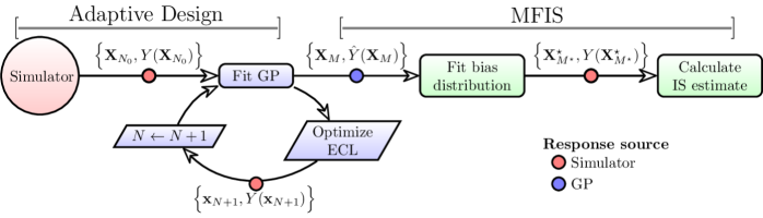
Figure 1: Full process combining ECL adaptive design with MFIS. Colored circles represent data with the response generated from the simulator (red) or GP (blue).

The remainder of the paper proceeds as follows. In Section 2, we provide the necessary background information regarding failure probability estimation, MFIS, and GP adaptive design. We introduce the ECL active learning strategy in Section 3. Section 4 showcases ECL empirically on a set of benchmark problems. Then we combine ECL designs with MFIS on a more involved and realistic, motivating application in Section 5, involving a reliability analysis for a NASA spacesuit design under impact loading. Section 6 provides a concluding discussion. Figure 1 provides a flowchart for our setup. Although some of the notation in that chart is not yet defined, we include it here because the flow mirrors the paper development as described above. We encourage the reader to refer back to this figure as related concepts are introduced in Section 2. Our main contribution (Section 3) comprises the cycle in blue; however it is motivated by the green sections, which are showcased on NASA’s spacesuit.

2 Reliability estimation tools

Here we provide the necessary context for estimating failure probability and contours.

2.1 Failure probability estimation

Consider an input–output system, modeled at high-fidelity with $\mathcal{T}:\mathcal{X}\equiv\mathbb{R}^{d}\rightarrow\mathbb{R}$ such that evaluations $\mathcal{T}(\mathbf{x})\rightarrow y$ are computationally/time intensive. Let $\mathbb{F}$ denote a distribution over $\mathbf{x}\in\mathcal{X}$, with density $f$, representing uncertainties in the inputs $\mathbf{x}$. Reliability is defined through a limit state function, $g:\mathbb{R}\rightarrow\mathbb{R}$, where failure is deemed to occur when $g(y)>0$ (Melchers and Beck, 2018). In engineering, a failure is often characterized as an output $y$ exceeding a certain threshold $T$, expressing the limit state function as $g(y)=y-T$. The failure region is characterized as

$$\mathcal{G}=\{\mathbf{x}\in\mathcal{X}:g(\mathcal{T}(\mathbf{x}))>0\},\quad\mbox{implying contour}\quad\mathcal{C}=\{\mathbf{x}\in\mathcal{X}:g(\mathcal{T}(\mathbf{x}))=0\}.$$ (1)

With indicator function $\mathds{1}$, the probability of failure ($\alpha$) is defined as

$$\alpha=\mathbb{E}_{X}[g(\mathcal{T}(\mathbf{x}))>0]=\int_{\mathbf{x}\in\mathcal{X}}\mathds{1}_{\{g(\mathcal{T}(\mathbf{x}))>0\}}\;d\mathbb{F}.$$ (2)

For technical/theoretical aspects of development in sequential design/active learning literature, the contour of interest $\mathcal{C}$ is sometimes assumed to be the zero contour, without loss of generality. However, our interest lies in identifying low/high quantiles of $\mathcal{T}(\mathbf{x})$, corresponding to a small $\alpha$. Our experience is that this setting is more challeging than zero or other more central contours in practice. We believe it is prudent to caution the reader against taking such liberties and arbitrarily describing $\mathcal{C}$.

Direct MC sampling is perhaps the most common numerical integration scheme for Eq. (2), yielding approximate estimator $\hat{\alpha}_{\text{MC}}$. With $M$ samples, $\mathbf{x}_{i}\stackrel{{\scriptstyle\mathrm{iid}}}{{\sim}}\mathbb{F}$, $i=1,\dots,M$, the MC estimate for $\alpha$ and its associated variance are

$$\hat{\alpha}_{\text{MC}} =\frac{1}{M}\sum_{i=1}^{M}\mathds{1}_{\{g(\mathcal{T}(\mathbf{x}_{i}))>0\}} \text{Var}\left(\hat{\alpha}_{\text{MC}}\right) =\frac{\hat{\alpha}_{\text{MC}}\left(1-\hat{\alpha}_{\text{MC}}\right)}{M}.$$ with (3)

While $\hat{\alpha}_{\text{MC}}$ in (3) is asymptotically unbiased (Robert and Casella, 2013), it can take $M$ in the millions to achieve a desirable accuracy, which might tax resources required for evaluation of $\mathcal{T}$. For example, if $\alpha=10^{-4}$ and we wish to have a root mean squared error (RMSE) of $10^{-6}$ (corresponding to $\text{Var}\left(\hat{\alpha}_{\text{MC}}\right)<10^{-12}$), $M>10^{8}$ samples are needed.

One solution to reducing this cost is through a focused simulation like importance sampling (IS). With IS, $\mathbf{x}^{\star}_{i}\stackrel{{\scriptstyle\mathrm{iid}}}{{\sim}}\mathbb{F}_{\star}$ are generated from an auxiliary distribution biased toward region(s) of inputs more likely to cause failure (i.e., land in $\mathcal{G}$). The resulting estimate

$$\hat{\alpha}_{\text{IS}}=P^{\text{IS}}(\mathbf{x}_{1}^{\star},\dots,\mathbf{x}^{\star}_{M^{\star}})=\frac{1}{M^{\star}}\sum_{i=1}^{M^{\star}}\mathds{1}_{\{g(\mathcal{T}(\mathbf{x}_{i}^{\star}))>0\}}w(\mathbf{x}_{i}^{\star})\quad\mbox{via weights}\quad w(\mathbf{x}^{\star})=\frac{f(\mathbf{x}_{i}^{\star})}{f_{\star}(\mathbf{x}_{i}^{\star})},$$ (4)

is asymptotically unbiased given $\text{supp}(f)\subseteq\text{supp}(f_{\star})$ (Robert and Casella, 2013, Section 14.2). Constructing bias distribution $\mathbb{F}_{\star}$ can be expensive in its own right, motivating the search for a cheaper low-fidelity model, like a surrogate $\mathcal{S}$.

Multifidelity importance sampling (MFIS) combines the low cost of generating samples from $\mathcal{S}$ when training the bias distribution in IS (Peherstorfer et al., 2016). Algorithm 1 shows pseudocode for MFIS: a bias distribution is generated by first evaluating $M$ samples with the cheap surrogate model $\mathcal{S}_{N}$, foreshadowing our notation for a GP surrogate (Section 2.2) which is trained on $N$ samples $\mathbf{X}_{N}\in\mathcal{X}$ paired with high-fidelity outputs $\mathbf{Y}_{N}$. Using the limit state function $g$, the samples that are classified to produce a failure response are used to train the bias distribution $\mathbb{F}_{\star}$ for IS. Peherstorfer et al., (2016) suggest using a Gaussian mixture model (GMM; Celeux and Govaert, 1995) for $\mathbb{F}_{\star}$. A set of $M^{\star}$ samples is drawn from $\mathbb{F}_{\star}$ and used to evaluate the high-fidelity model. The associated responses $\mathbf{Y}_{M^{\star}}$ are used along with IS weights $\mathbf{w}_{M^{\star}}$ to yield failure probability estimate $\hat{\alpha}^{\text{MFIS}}$.

Algorithm 1 Multifidelity Importance sampling

1:procedure MFIS($\mathcal{T}$, $\mathcal{S}_{N}$, $\mathbb{F}$, $\mathbb{F}_{\star}$, $M$, $M^{\star}$, $\kappa$)

2:     Draw $M$ samples $\mathbf{X}_{M}=\{\mathbf{x}_{1},\dots,\mathbf{x}_{M}\}$ from $\mathbb{F}$

3:     $\hat{\mathbf{Y}}_{M}\leftarrow\mathcal{S}_{N}(\mathbf{X}_{M})$          ## Predictions from surrogate

4:     Train a GMM of $\kappa$ clusters with set $\mathcal{F}=\{\mathbf{x}\in\mathcal{X}:g(\hat{y}(\mathbf{x}))>0\}$         ## Form $\mathbb{F}_{\star}$

5:     Draw $M^{\star}$ samples $\mathbf{X}^{\star}_{M^{\star}}=\{\mathbf{x}^{\star}_{1},\dots,\mathbf{x}^{\star}_{M^{\star}}\}$ from $\mathbb{F}_{\star}$

6:     $\mathbf{w}_{M^{\star}}=\Big{[}\frac{f(\mathbf{x}^{\star}_{1})}{f_{\star}(\mathbf{x}^{\star}_{1})},\dots,\frac{f(\mathbf{x}^{\star}_{M^{\star}})}{f_{\star}(\mathbf{x}^{\star}_{M^{\star}})}\Big{]}$          ## Compute importance weights

7:     $\mathbf{Y}_{M^{\star}}\leftarrow\mathcal{T}(\mathbf{X}^{\star}_{M^{\star}})$          ## Evaluate high-fidelity model

8:     $\hat{\alpha}_{\text{MFIS}}=\frac{1}{M^{\star}}\sum_{i=1}^{M^{\star}}\mathbb{I}_{g(y_{i})>0}w(\mathbf{x}^{\star}_{i})$         ## MFIS estimate through (4)

9:     return $\hat{\alpha}_{\text{MFIS}}$

10:end procedure

MFIS seeks to preserve the unbiasedness of the estimator (4) while minimizing the number of high-fidelity evaluations $M^{\star}$. Yet the question of how to train a $\mathcal{S}_{N}$ for MFIS is not widely discussed in the literature. As a simple experiment, we conduct MFIS with the GP $\mathcal{S}_{N}$ on the Ishigami function (Ishigami and Homma, 1990): $\mathcal{T}^{\text{Ish}}(\mathbf{x})=\sin(x_{1})+5\sin^{2}(x_{2})+0.1x_{3}^{4}\sin(x_{1})$ for $\mathbf{x}\in[-\pi,\pi]^{3}$. $\mathcal{T}^{\text{Ish}}$ is smooth, with six global minima creating six disjoint failure regions. We define the failure region $\mathcal{G}^{\text{Ish}}$ for values $y$ below the threshold $T=-9.2244$. To align this with our definition in (1), let $g^{\text{Ish}}(y)=-y+9.2244$, which corresponds to $\alpha^{\text{Ish}}\approx 0.001$. In our experiment, we studied estimates of $\alpha^{\text{Ish}}$ for increasing budgets of simulator evaluations in an MC exercise with fifty repeats.

The left panel of Figure 2 shows errors $|\hat{\alpha}-\alpha^{\text{Ish}}|$ for three comparators with the dark lines indicating means, and 95% confidence interval (CI) as shaded bands. A simple MC estimate $\hat{\alpha}_{\text{MC}}$ from (3) is along the green dotted line; observe that its absolute error decreases as the number of high-fidelity samples ($M$ on the $x$-axis) increases, showing a slow convergence to the truth (zero error). The blue dashed line represents MFIS-based estimates from (4) using a GP $\mathcal{S}_{N}$ trained on $N=200$ space-filling Latin Hypercube samples (LHS; Mckay et al., 1979) generating evaluations of the simulator $\mathcal{T}^{\text{Ish}}$, followed by $M^{\star}$ draws from $\mathbb{F}_{\star}$ (with $N+M^{\star}$ on the $x$-axis). Finally, the red solid line represents the GP trained via our proposed entropy-based adaptive design (30 LHS followed by 170 acquisitions; details in Section 3). Notice that the red solid line starts better than both (small $M^{\star}$) and, unlike the blue dashed line, offers noticeable further improvement (larger $M^{\star}$).

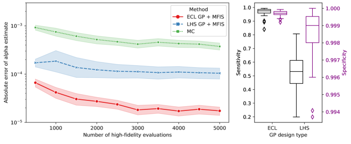
Figure 2: Left: Absolute errors of failure estimates (truth is $10^{-4}$) for the Ishigami function. Bold lines denote mean error over 50 samples with shading for the 95% confidence regions. Right: failure region classification statistics across 50 MC repeats for the two GPs.

The right panel of Figure 2 shows the proportion of the input space that is correctly classified as being inside (black/left $y$-axis) and outside (magenta/right) the failure region. This calculation is based on a $10^{6}$-sized LHS in the 3d input space. Observe that the LHS-based GP produces considerably inferior estimates. The adaptive method correctly identifies most of failure points (sensitivity) and nearly all of the non-failure points (specificity). GPs trained on space-filling LHSs often miss some of the failure regions, resulting in a much lower sensitivity. Lower specificity in the LHS option means that more locations that are not failures are being labeled as such. If used for MFIS, the result would be a flawed biasing, leading to inefficient reliability estimates.

2.2 Adaptively designed Gaussian processes surrogates

GPs make popular surrogates due to their tremendous flexibility in modeling complex surfaces (Sacks et al., 1989; Santner et al., 2018; Gramacy, 2020). They may be simply characterized by placing a multivariate normal (MVN) prior on the observations/outputs $\mathbf{Y}_{N}$. MVNs are uniquely defined by a mean vector $\mu$, often assumed to be zero in the GP regression context for simplicity, and an $N\times N$ covariance matrix $\mathbf{K}_{N}$. For $N$ observations included in $D_{N}=(\mathbf{X}_{N},\mathbf{Y}_{N})$, the joint model for the responses is $\mathbf{Y}_{N}\sim\mathcal{N}_{N}(\mathbf{0},\mathbf{K}_{N})$. Entries of $\mathbf{K}_{N}$ are calculated from a kernel $k_{\Psi}(\mathbf{x}_{i},\mathbf{x}_{j})$, which is usually based on inverse distances in the input space. Many expressions of $k_{\Psi}(\cdot,\cdot)$ exist, including the squared exponential and Matérn families (Stein, 2012). The kernel hyperparameters $\Psi$, such as $\tau^{2}$ (scale) and $\theta$ (lengthscale), are estimated by optimizing the MVN log-likelihood.

The true power of a GP lies in its ability to produce accurate predictions by conditioning on observed data. The predictive equations for a new testing location $\mathbf{x}^{\prime}$ are:

$$\begin{split}\mu_{N}(\mathbf{x}^{\prime}|D_{N})&=\mathbf{k}(\mathbf{x}^{\prime},\mathbf{X}_{N})\mathbf{k}(\mathbf{X}_{N},\mathbf{X}_{N})^{-1}\mathbf{Y}_{N}\\ \sigma_{N}^{2}(\mathbf{x}^{\prime}|D_{N})&=k_{\Psi}(\mathbf{x}^{\prime},\mathbf{x}^{\prime})-\mathbf{k}(\mathbf{x}^{\prime},\mathbf{X}_{N})\mathbf{k}(\mathbf{X}_{N},\mathbf{X}_{N})^{-1}\mathbf{k}(\mathbf{x}^{\prime},\mathbf{X}_{N})^{\top},\end{split}$$ (5)

where $\mathbf{k}(\mathbf{x}^{\prime},\mathbf{X}_{N})$ is the vector of cross evaluations of the kernel $k_{\Psi}(\cdot,\cdot)$ between $\mathbf{x}^{\prime}$ and $\mathbf{X}_{N}$. When we write $\mathcal{S}_{N}$ we are referring to these equations without a particular $\mathbf{x}^{\prime}$ in mind. A GP’s ability to produce fast, accurate predictions has fueled the rise of active learning (i.e. sequential design) techniques in the machine learning community (Settles, 2011). The idea is to leverage the current model’s information (fit to existing data) to greedily select the next sample/batch of inputs used to gather more data, updating that information. Making such selections relies on the optimization of an acquisition function. A litany of acquisition functions serve diverse modeling goals. These include minimizing predictive variance (MacKay, 1992; Seo et al., 2000; Cohn, 1994), finding function optima (Jones et al., 1998; Gramacy, 2011; Wu et al., 2017) via so-called Bayesian optimization (BO), and accurate hyperparameter optimization (Gramacy and Apley, 2015; Zhang et al., 2021).

Targeting level sets

Several acquisition functions target level sets, or contours, and are tailored to GP regression. For our purposes, the contour of interest is the boundary of the failure region(s) in (1). Some acquisition functions focus squarely on sampling where $\mathcal{C}$ is uncertain (Bect et al., 2012; Echard et al., 2010; Ranjan et al., 2008; Bichon et al., 2008; Lee and Jung, 2008). Others are inspired by BO solutions, striking a balance between extrema-seeking and global posterior uncertainty (Bryan and Schneider, 2008; Gotovos, 2013; Bogunovic et al., 2016). When applying contour finding for failure probability estimation, it is vital to identify all disjoint regions within $\mathcal{C}$ (when more than one exist). Therefore, it is highly desirable for an adaptive design method to promote exploration. Consequently many acquisition functions involve integrating over the domain $\mathcal{X}$ (Ranjan et al., 2008; Bichon et al., 2008; Picheny et al., 2010; Chevalier et al., 2013, 2014). We know of no examples where such integrals that can be evaluated analytically. Numerical schemes, based on reference grids and other quadrature, do not scale well to large dimension $d$. Some shortcuts are helpful, e.g., Lyu et al., (2021) leverage predictive variance in (5) to simplify some aspects. However, challenges remain to produce a method tractable for estimating a small-volume contour in a big $\mathcal{X}$.

A complimentary class of approaches involve identifying $\mathcal{C}$ by mapping to a classification setting (Gotovos, 2013; Azzimonti et al., 2016; Bolin and Lindgren, 2015). A common measure of uncertainty for discrete random variables is entropy. Originating from information theory (Cover, 2006), the entropy of a discrete random variable $W$ is measured as

$$H(W)=-\sum_{i=1}^{k}\mathbb{P}(w_{i})\log\mathbb{P}(w_{i}),$$ (6)

where $i={1,\dots,k}$ indexes events $w_{i}$, with probability mass $\mathbb{P}(w_{i})$. A mapping that would apply in our setting, as a criterion for valuing inputs $\mathbf{x}$, is with $k=2$ where

$$w_{1}(\mathbf{x})\equiv\{\mathbf{x}\in\mathcal{G}_{N}\}\quad\text{and}\quad w_{2}(\mathbf{x})\equiv\{\mathbf{x}\in\mathcal{G}_{N}^{\mathsf{c}}\}.$$ (7)

Here, $\mathcal{G}_{N}$ is an estimate of the failure region in (1), say via GP $\mathcal{S}_{N}$ predictive equations in (5). We shall be more precise momentarily. Abusing notation slightly, this $H(W)$ would highly value inputs $\mathbf{x}$, via larger entropy, which are close to $\mathcal{C}_{N}$, the (estimated) boundary of $\mathcal{G}_{N}$, i.e., such that $\mathbb{P}(w_{1})\approx\mathbb{P}(w_{2})\approx 1/2$, which is sensible.

Oakley, (2004) considered entropy for choosing among candidate LHSs in the second step of a two-stage design setup, whereas we consider a pure-sequental setup where the number of stages is proportional to the desired design size. They targeted output quantiles, like 95%, implicitly defining $\mathcal{C}$ and thus $\mathcal{G}$ and their GP-estimated analogues. We are interested in much larger quantiles, such that any LHS candidate would have low probability of being nearby $\mathcal{G}_{N}$, mirroring a calculation similar to that in Eq. $\eqref{eq:monte_carlo}$. Contour Location Via Entropy Reduction (CLoVER; Marques et al., 2018) greedily maximizes the reduction in contour entropy through a lookahead scheme. As in several other methods, CLoVER relies on a set of reference points or knots in $\mathcal{X}$ for numerical integration. But knots are problematic for reasons similar to the LHS candidates above: hard to get enough nearby/inside the failure region. More knots do not help much because the expense of quadrature is squared.

3 Entropy-based Adaptive Design

MFIS holds the potential to leverage a cheaper surrogate to obtain unbiased reliability estimates, but only if the surrogate is accurate around $\mathcal{C}$. Here we propose an entropy-based contour locator (ECL) acquisition function toward that goal.

3.1 Entropy acquisition function

After being fit to training data $D_{N}$, our GP surrogate $\mathcal{S}_{N}$ provides a distribution in (5) for $Y(\mathbf{x})$. In the case of a failure region $\mathcal{G}$ defined by affine limit state function $g$, the entropy (6) with discrete events (7) for input $\mathbf{x}$ relative to estimate $\mathcal{G}_{N}$ via $\mathcal{S}_{N}$ is

$$\mathrm{ECL} (\mathbf{x}\mid\mathcal{S}_{N},g)=$$ (8)

$$-\mathbb{P}\Big{(}g(Y(\mathbf{x}))>0\Big{)}\log\mathbb{P}\Big{(}g(Y(\mathbf{x}))>0\Big{)}-\mathbb{P}\Big{(}g(Y(\mathbf{x}))\leq 0\Big{)}\log\mathbb{P}\Big{(}g(Y(\mathbf{x}))\leq 0)\Big{)}$$

$$=-\left(1-\Phi\left(\frac{\mu_{N}(\mathbf{x})-T}{\sigma_{N}(\mathbf{x})}\right)\right)\log\left(1-\Phi\left(\frac{\mu_{N}(\mathbf{x})-T}{\sigma_{N}(\mathbf{x})}\right)\right)$$

$$\qquad\qquad-\Phi\left(\frac{\mu_{N}(\mathbf{x})-T}{\sigma_{N}(\mathbf{x})}\right)\log\left(\Phi\left(\frac{\mu_{N}(\mathbf{x})-T}{\sigma_{N}(\mathbf{x})}\right)\right),$$

where $\Phi$ is the standard univariate Gaussian CDF. Noting the symmetry in (8), this would work identically for any $g(y)=a(y-T)$ where $a\in\{-1,1\}$, meaning that the underlying criterion is unchanged when searching for extremely small, rather than large, thresholds. Also, ECL trends higher as the GP’s predicted mean $\mu_{N}(\mathbf{x})$ moves closer to the threshold or $\sigma_{N}(\mathbf{x})$ is higher, facilitating an exploration–exploitation trade off. ECL is maximized when $\mathbb{P}(g(Y(\mathbf{x}))>0)=\mathbb{P}(g(Y(\mathbf{x}))\leq 0)=1/2$, targeting $\mathbf{x}\in\mathcal{C}_{N}\equiv\{\mathbf{x}:g(\mu_{N}(\mathbf{x}))=0\}$.

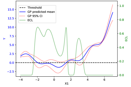
Figure 3: GP surrogate predictions and ECL values for the multimodal function along $x_{2}=5.8$.

To explore the ECL surface, consider a 2d multimodal function (Bichon et al., 2008):

$$\mathcal{T}^{\text{MM}}(\mathbf{x})=\frac{(x_{1}^{2}+4)(x_{2}-1)}{20}-\sin\left(\frac{5x_{1}}{2}\right)-2,$$ (9)

where $x_{1}\in[-4,7],x_{2}\in[-3,8]$. This function has been used for reliability/level-set finding with $T=0$ (Bichon et al., 2008; Marques et al., 2018). We trained a GP on an LHS of $N=20$ points. Figure 3 shows the predictive mean ($\mu_{N}(\mathbf{x})$ blue line), 95% mean confidence interval (roughly $\pm 2\sigma_{N}(\mathbf{x})$, red dotted lines) and ECL (green line) across the slice $x_{2}=5.8$. Since $g(\mu_{N}(\mathbf{x}))$ crosses zero twice, there are two global maxima of ECL in this slice alone, along with several other local maxima where the upper bound of the confidence bound is close to or above zero. In higher volume input spaces the dimension of the manifold tracing out the level set also increases, resulting in a continuum of ridges in the ECL surface. If you want to look ahead, Figure 4 provides a visual. Such a surface could present challenges to effective numerical optimization for the purpose of solving for adaptive design acquisitions.

3.2 Optimization-based acquisition

To address the (potentially) multimodal nature of ECL in (6), as illustrated in Figure 3, we developed a two-step strategy to solving for each greedy acquisition:

$$\mathbf{x}_{N+1}=\mathrm{argmax}_{\mathbf{x}\in\mathcal{X}}\mathrm{ECL}(\mathbf{x}\mid\mathcal{S}_{N}).$$

In the first stage we optimize over a discrete-space-filling candidate set $\bar{\mathbf{X}}_{N_{c}}$. We prefer LHS candidates with $N_{c}\approx 10d$, following the rule of thumb proposed in Loeppky et al., (2009). Then, in the second stage, we use this global, but coarse, solution to initialize a local solver, such as BFGS (Byrd et al., 1995). The first stage is designed to “select” a global domain of attraction, while the second stage ascends that peak of the ECL surface.

Algorithm 2 Entropy Optimization

1:procedure Entropy.Opt($N_{c},\mathcal{S}_{N},\mathcal{X}$)

2:     $\bar{\mathbf{X}}_{N_{c}}\leftarrow$ LHS of size $N_{c}$ in $\mathcal{X}$          ## Candidate set

3:     $\check{\mathbf{x}}\leftarrow\mathrm{argmax}_{\bar{\mathbf{x}}\in\bar{\mathbf{X}}_{N_{c}}}\;\mathrm{ECL}(\bar{\mathbf{x}}\mid\mathcal{S}_{N})$          ## Discrete search

4:     $\mathbf{x}_{N+1}\leftarrow\mathrm{argmax}_{\mathbf{x}\in\mathcal{B}(\check{x})}\;\mathrm{ECL}(\mathbf{x}\mid\mathcal{S}_{N})$          ## Continuous, local, from $\check{\mathbf{x}}$

5:     return $\mathbf{x}_{N+1}$

6:end procedure

The details are laid out in pseudocode in Algorithm 2. In line 4, representing stage 2 local search, the scope is based on $\check{\mathbf{x}}$. For a true local search, the region $\mathcal{B}(\check{\mathbf{x}})$ may comprise of a box containing $\check{\mathbf{x}}$ whose sides extend to nearby elements of the candidate set $\bar{\mathbf{X}}_{N_{c}}$ or to the edge of $\mathcal{X}$, whichever is closer. Such narrowed scope may help local optimizers that support box constraints, like BFGS does. In our implementation (more details in Section 4.1) simply take $\mathcal{B}(\check{\mathbf{x}})=\mathcal{X}$, the whole space, and use $\check{\mathbf{x}}$ to initialize the search.

We find that the stochastic and coarse global nature of the first stage (owing to the small LHS), paired with a precise and focused second stage, brings benefits beyond avoiding solutions trapped in vastly inferior local maxima. Sometimes the surrogate $\mathcal{S}_{N}$ becomes over-confident about its predictive equations, leading to small $\hat{\sigma}(\mathbf{x})$ nearby an estimated failure region contour $\mathcal{C}_{N}$ that is far from the true $\mathcal{C}$. In such situations, the first stage offers potential to ignore that area for local maxima in a less seductive, but almost-as-good region. Injecting a degree of stochasticity into optimization is a convenient way of avoiding pathologies, building-in robustness (Wolpert and Macready, 1997).

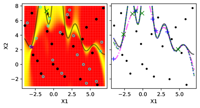
Figure 4: Left: ECL surface based on a GP fit to $N_{0}=20$ points (black circles). The true $\mathcal{C}^{\text{MM}}$ is denoted by the black curve. Candidates $\mathbf{X}_{N_{C}}$ are aqua open circles, with $\check{\mathbf{x}}$ at the terminus of an arrow pointing to $\mathbf{x}_{N_{0}+1}$, the optimized selection as green ‘$\times$’. The purple star shows the best of these from all candidates. Right: zero contours based on initial GP fit ($\mathcal{S}_{N_{0}}$ pink dot-dashed curve), at $\mathcal{S}_{N_{0}+5}$, after five ECL sequentially selected points (green $\times$’s/dashed), and similarly after a single $N_{b}=5$ batch $\mathcal{S}_{N_{0}+N_{b}}$ (blue pluses/dotted curve).

An illustration on the 2d multimodal function (9) is provided in the left panel of Figure 4. Here we show the ECL surface based on a GP $\mathcal{S}_{N}$ fit to the same $N_{0}=20$ points as used for Figure 3. The multimodal function’s true zero contour ($\mathcal{C}^{\text{MM}}$) is shown with the black curve. Observe that the highest ECL regions (yellow) are near that contour. Other local maxima are present where there is little data (bottom left corner) and $\mathcal{S}_{N}$’s uncertainty high. Aqua blue open circles indicate the candidate set $\bar{\mathbf{X}}_{20}$. The arrow pointing from one blue circle to the green ‘$\times$’ denotes the chosen candidate point $\check{\mathbf{x}}$ from the first stage and the resulting $\mathbf{x}_{N+1}$ after continuous optimization in the second. Notice that the green ‘$\times$’ is different from the purple star, the optimal location if local optimization is conducted on all 20 candidates. The green ‘$\times$’ finds an almost-as-good region that is close to $\mathcal{C}$.

Although technically (slightly) sub-optimal for the individual acquisition of $\mathbf{x}_{N+1}$, we think that the view in Figure 3 (left) suggests that the solution we found (green ‘$\times$’) is indeed sensible. The first stage is more likely to target a high uncertainty region, with a wider domain of attraction (more yellow), due to its coarse nature. Ideally, the attractiveness of “big yellow” regions would be captured formally by the acquisition criteria. This is why most authors integrate over the input space, but that requires numerical quadrature which we are trying to avoid. Our two-stage scheme is simpler to implement, and as results shown later in Section 4.2 support, fast in execution and robust in a loose sense.

3.3 Batch selection

Modern high-performance computing (HPC) resources allow simulations to be run in parallel. To accommodate, here we extend our ECL adaptive design strategy to batch acquisition. Suppose we wish select a batch of $N_{b}$ samples, e.g., to saturate the node of a computing cluster. One option is to extend our criteria in (8) from singular $\mathbf{x}$ to multiple $\mathbf{X}_{N_{b}}$, in the spirit of Zhang et al., (2020) for variance-based acquisition. This is doable by upgrading surrogate $\mathcal{S}_{N}$ pointwise predictive equations in (5) to joint ones. Similar MVN conditioning applies, e.g., see Eq. (5.3) in Gramacy, (2020). Next, calculate entropy in (6) on the resulting MVN. You will still get a closed form (not shown) up to multivariate CDF evaluations $\Phi_{N_{b}}$. Calculating $\Phi_{N_{b}}$ can pose a challenge. Although univariate $\Phi$ involve a degree of quadrature, evaluation is so fast and accurate (and built-in as native in most programming languages) that we generally regard it as analytic in practice. Multivariate $\Phi_{N_{b}}$, involving high dimensional quadrature in vast “tail volumes”, is much more challenging, see Genz and Bretz, (2009). Although software is available for R (Genz et al., 2019), we find that $N_{b}$ on the scale of the number of cores in supercomputers (e.g., $N_{b}=16$ or bigger), evaluation is slow and with accuracy that can be problematic for downstream library-based optimization via methods, e.g., via BFGS.

Instead we prefer to select batch elements sequentially, updating $\mathcal{S}_{N}\rightarrow\mathcal{S}_{N}^{(+1)}$ to account for each new selected input (but not its response) in the batch until we reach $\mathcal{S}_{N}^{(+N_{b})}$. Specifically, given $0\leq n_{b}\leq N_{b}$ selections so far, we may deduce the following equations for $\mathcal{S}_{N}^{(+n_{b})}$, where $\mathbf{X}_{N+n_{b}}=\mathbf{X}_{N}\cup\mathbf{X}_{n_{b}}$ and with $\mathbf{X}_{0}\equiv\emptyset$ reducing to the following using (5):

$$\mu_{N}^{(+n_{b})}(\mathbf{x}^{\prime}|\mathbf{X}_{N+n_{b}},\mathbf{Y}_{N}) =\mu_{N}(\mathbf{x}^{\prime}|\mathbf{X}_{N},\mathbf{Y}_{N})=\mathbf{k}(\mathbf{x}^{\prime},\mathbf{X}_{N})\mathbf{k}(\mathbf{X}_{N},\mathbf{X}_{N})^{-1}\mathbf{Y}_{N}$$ (10)

$$\sigma^{2(+n_{b})}_{N}(\mathbf{x}^{\prime}|\mathbf{X}_{N+n_{b}},\mathbf{Y}_{N}) =k_{\Psi}(\mathbf{x}^{\prime},\mathbf{x}^{\prime})-\mathbf{k}(\mathbf{x}^{\prime},\mathbf{X}_{N+n_{b}})\mathbf{k}(\mathbf{X}_{N+n_{b}},\mathbf{X}_{N+n_{b}})^{-1}\mathbf{k}(\mathbf{x}^{\prime},\mathbf{X}_{N+n_{b}})^{\top}.$$

Each of these updates $\mathcal{S}_{N}^{(+n_{b})}\rightarrow\mathcal{S}_{N}^{(+n_{b}+1)}(\mathbf{x}_{n_{b}+1})$, in particular for $\sigma^{2(+n_{b})}(\mathbf{x})$ as $n_{b}\rightarrow n_{b}+1$ with new acquisition $\mathbf{x}_{n_{b}+1}$ augmenting $\mathbf{X}_{n_{b}}$ to build $\mathbf{X}_{n_{b}+1}$, can be performed in time quadratic in $N+n_{b}$ via partition inverse equations (Barnett, 1979; Gramacy and Polson, 2011; Gramacy, 2020, Section 6.3). However, the otherwise cubic burden is often manageable in active learning where the whole enterprise is focused on making $N$ as small as possible.

Algorithm 3 Batch Entropy

1:procedure Entropy.Batch($\mathcal{S}_{N}$, $N_{b}$, $N_{c}$, $\mathcal{X}$)

2:     ${\mathcal{S}}_{N}^{(+0)}\leftarrow\mathcal{S}_{N}$          ## Initialize deduced surrogate

3:     for $n_{b}=1,\dots,N_{b}$ do

4:         $\mathbf{x}_{n_{b}}\leftarrow\text{\sc Entropy.Opt}(\mathcal{S}_{N}^{(+n_{b}-1)},N_{c},\mathcal{X})$          ## Select next point (Alg. 2)

5:         $\mathcal{S}_{N}^{(+n_{b})}\leftarrow\mathcal{S}_{N}^{(+n_{b}-1)}(\mathbf{x}_{n_{b}})$          ## Update variance Eq. (10) in GP

6:     end for

7:     return ${\mathbf{X}}_{N_{b}}\equiv[\mathbf{x}_{1}^{\top},\dots,\mathbf{x}_{N_{b}}^{\top}]^{\top}$          ## Return batch of $N_{b}$ design points

8:end procedure

With $\mathcal{S}_{N}^{(+N_{b})}$ defined in this way, batch selection becomes an exercise in repeated greedy selection. This is detailed in Algorithm 3, with Algorithm 2 deployed as a subroutine. It is worth remarking that a new candidate set $\bar{\mathbf{X}}_{N_{c}}$ is generated for each new call of line 4. If we were to rely upon the same candidate set for the entire batch, we would in effect be taking the $N_{b}$ best candidate points, some of which could be far from the local maxima regions of interest. It is possible (although in practice uncommon) that some of the acquisitions are very close to others in the same batch. Since we operate under the assumption that the high-fidelity model is deterministic, replicates are not helpful. In our implementation (more in Section 4.1), we account for this by reverting to the optimal candidate point $\check{\mathbf{x}}$ for $\mathbf{x}_{n_{b}}$ in such cases, undoing the stage 2 local search. At the end of the batch, new simulations must be performed at $\mathbf{X}_{N_{b}}$, forming $\mathbf{Y}_{N_{b}}$, combining with $D_{N}$ to obtain $D_{N+N_{b}}$. Inference follows for any hyperparameters $\Psi$ required to form $\mathcal{S}_{N+N_{b}}$ which is, of course, different than the intermediate $S_{N}^{(+n_{b})}$ which may be discarded after each iteration of the loop.

To illustrate, we return to the multimodal example of Section 3.2. The right panel of Figure 4 compares the acquisition of five runs one-at-a-time (i.e., multiple single acquisitions with updates) and five as a batch. The dash-dotted pink line shows the GP’s predicted mean contour via $\mathcal{S}_{N_{0}}$ before either adaptive design. The green $\times$’s were selected one at a time, leading to the green dashed $\mathcal{C}_{N+5}$ contour. In a similar fashion, the blue $+$’s and dotted curve represent the results from the batch size of 5. Both adaptive designs select the same first point (close to (-1.25, 7.2)); this is guaranteed by using the same candidate set. In the batch design, only the GP’s variance equation is updated, which results in runs being selected close to the original GP’s zero contour were ECL is maximized. In contrast, repeated one-at-a-time acquisition allows updating of the mean surface. Yet surprisingly, the resulting contours from both designs (green dashed and blue dotted lines) are fairly similar and capture $\mathcal{C}^{\text{MM}}$ well. This mirrors other work on batch active learning with GPs (Zhang et al., 2020); little is lost on the batch setting versus its purely greedy analog.

4 Implementation and benchmarking

Now we provide results for a series of experiments showcasing ECL, and contrasting against existing contour-finding acquisition functions. We first detail our implementation and the synthetic simulators used in the experiments. Then we present and discuss results of MC sequential design exercises in terms of sensitivity and relative error of the failure region’s volume based on GP predictions in (5) over acquisition iterations.

All analysis was performed on a six-core hyperthreaded Intel i7-9850H CPU at 2.59GHz. Python and R code (R Core Team, 2021) supporting our methodological contribution, and all examples reported here and throughout the paper, may be found on our Git repository.

https://bitbucket.org/gramacylab/nasa/src/master/entropy

4.1 Implementation and synthetic data

The following implementation details are noteworthy. Our methodological contribution is encapsulated in the Python package eclGP, incorporating GP functionality from the sklearn package (Pedregosa et al., 2011). For all of our synthetic examples, we privilege a separable Gaussian kernel formulation, although other forms such as Matérn (Stein, 2012) could easily be used. To ensure stability in the calculation of the inverse of the covariance matrix, we fix a jitter (Neal, 1998) of $10^{-6}$.

We compare the ECL-based estimates of a contour $\mathcal{C}$ to established contour finding acquisition functions with publicly available code. For CLoVER, we utilize the Python code accompanying Marques et al., (2018), with the only adjustment being setting the candidate and integration knots to LHSs of size 1000 for each experiment (see Appendix A for a discussion). Implementations for all other methods leverage the R package KrigInv (Chevalier et al., 2014), using the "genoud" option for optimization and the recommended defaults for constructing integration knots where relevant (SUR, tIMSE). In R, we rely on DiceKriging (Roustant et al., 2012) to fit GPs.

Function	$\mathcal{X}$	$N_{0}$	$N$	$g(y)$	vol($\mathcal{G}$)	Quantile
Branin-Hoo	$[-5,10]\times[0,15]$	10	30	$y-206$	2.1783	0.9903
Ishigami	$[-\pi,\pi]^{3}$	30	200	$-y+10.244$	0.0250	0.9999
Hartmann-6	$[0,1]^{6}$	60	500	$y-2.63$	0.0011	0.9989

Table 1: The design space, allocation of samples, limit state functions, volume of the failure region, and quantiles for the synthetic tests.

Experiments are conducted on the Branin-Hoo (Forrester et al., 2008), Ishigami (Ishigami and Homma, 1990), and Hartmann-6 (Surjanovic and Bingham, 2014) functions. Table 1 provides a summary of the experiments, including the number of sample points $N$ and limit state functions $g(\cdot)$ used to define failure regions $\mathcal{G}$. The limit state functions are defined so that $\mathcal{G}$ for each function contains at least two local extremes located in disjoint failure regions. The volume of $\mathcal{G}$ is less than 1% of the total volume of the design region in each instance. Volumes reported in the table are based on averaging 100 MC estimates from LHSs of size $10^{6}$. Dense testing LHSs were used to calculate sensitivity and predicted volume of the failure region out-of-sample. For Branin-Hoo an LHS of $5\times 10^{6}$ points is used for prediction/classification, whereas Ishigami and Hartmann-6 used $10^{7}$. To initialize the sequential design we follow the rule of thumb for setting $N_{0},N_{c}=10d$ (Loeppky et al., 2009), except for the 2d Branin-Hoo where $N_{0}=10$ was sufficient.

4.2 Synthetic tests for contour finding

Earlier in Figure 2, when motivating adaptive design strategies for contour location, we showcased results on the Ishigami function. Those showed that using an ECL design of 200 points provides a GP predictive mean that produces much higher sensitivity and specificity than a GP trained on an LHS of the same size. Here we expand that analysis against benchmarks. Figure 5 augments with other test functions and the following competitors: EGRA (Bichon et al., 2008), Ranjan (Ranjan et al., 2008), and tMSE (Picheny et al., 2010) as strategies that use closed-form calculations for continuous optimization acquisition; CLoVER (Marques et al., 2018), SUR (Chevalier et al., 2014) and tIMSE (Picheny et al., 2010) require integral approximation.

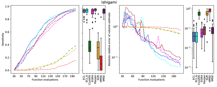
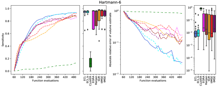
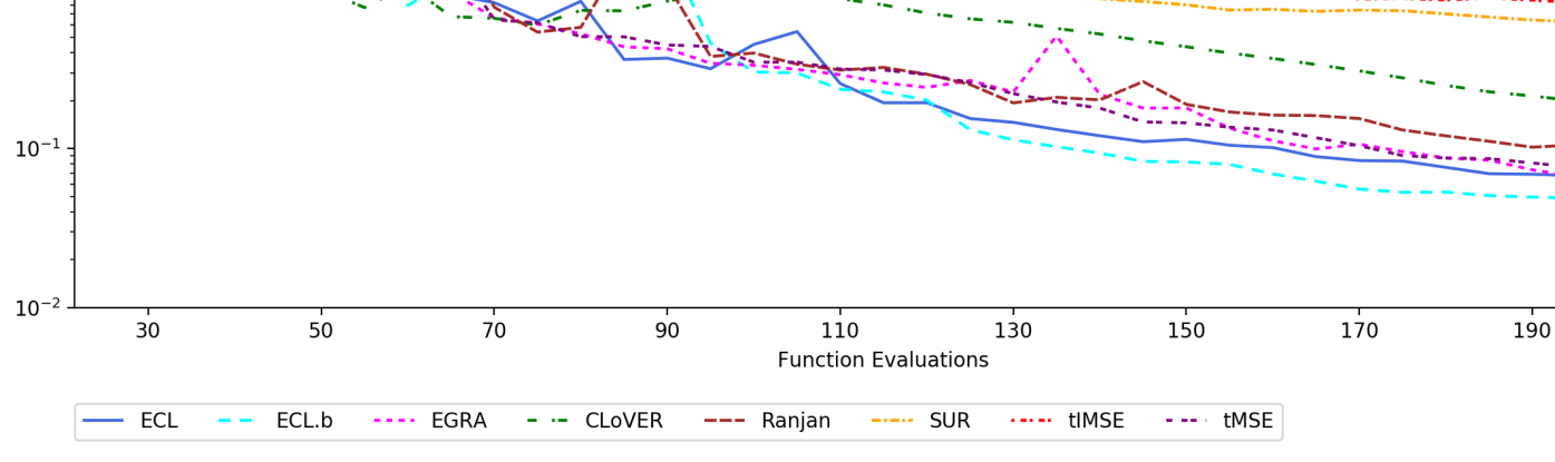
Figure 5: Comparing sequential designs in 30 MC repetitions. Left: mean sensitivity classifying failure region $\mathcal{G}$. Middle left: distributions of sensitivity after last acquisition. Middle right: mean relative error $\mathrm{vol}(\mathcal{G})$. Right: final distributions of relative volume error.

The figure tracks sensitivity as design size increases (left) and provides a boxplot of the final distribution of sensitivity (middle left). Similarly, relative error for $\mathrm{vol}(\hat{\mathcal{G}})$ is tracked (middle right), followed by its final distribution error (right). Thirty MC repetitions were conducted for each experiment, with the line plots displaying means. Across all three experiments (rows in the figure) our ECL method is among the best achievers in terms of sensitivity (higher is better) and volume error (lower is better).

For Branin-Hoo, ECL and CLoVER – the entropy-based methods – distinguish themselves early on in the adaptive design in both sensitivity and volume error compared to all other methods. By the end of the experiment, all methods have a similar sensitivity. ECL’s volume error is in line with the integration methods, beating its closed-form competitors. For Ishigami, observe that final mean sensitivity for ECL is bested by Ranjan. Yet when it comes to the relative error of the contour’s volume, ECL is far below that of Ranjan. Hartmann-6 imposes challenges in higher input dimension, which is why we extend the adaptive design to 500 total points. In this experiment, we find that the explorative nature of ECL is key to finding the failure contour. The bottom row of Figure 5 shows that ECL provides a much more robust design with high sensitivity and a volume error nearly an order of magnitude smaller than others. We also created a batch ECL design (ECL.b) with batch sizes of 5 for Branin-Hoo and 10 for Ishigami and Hartmann-6. In all three experiments, ECL.b performs similarly to ECL.

For the methods that rely upon a “grid” of integration knots (CLoVER, SUR, tIMSE), the size of that grid greatly affects their ability to explore and identify parts of the failure contour. With a set of 1000 knots for Branin-Hoo, CLoVER performs very well – reaching a high sensitivity plateau before the other methods. Yet when the same number of knots is used in the 3d or 6d problems with a higher quantile, it struggles. In a similar way, the combination of multiple failure regions (six) and a high quantile for the Ishigami experiment poses a great challenge for SUR and tIMSE. See Appendix A for further discussion.

Method	ECL	ECL.b	CLoVER	EGRA	Ranjan	SUR	tIMSE	tMSE
Branin-Hoo	0.008	0.002	0.42	0.2	0.2	0.4	0.3	0.2
Ishigami	0.10	0.08	17.8	3.9	4.5	3.5	3.4	3.9
Hartmann-6	4.40	0.78	428.4	66.0	59.2	109.1	111.7	59.5

Table 2: Average computation times (minutes) to select points across MC 30 repetitions.

Table 1 summarizes average computation time to build one full sequential design for each method. The timings include acquisition efforts and subsequent GP updating. Scripts for ECL, ECL.b and CLoVER are in Python and the rest are in R. Note the speed at which ECL and ECL.b adaptive designs are built, especially compared to methods using numerical quadrature (CLoVER, SUR, and tIMSE). ECL provides between one and two orders of magnitude speedup. Using a batch size of 10 cuts the average computation time of ECL by five for the Hartmann-6 experiment, while still providing designs with similar sensitivity and volume error.

5 Failure probability estimation

Here we transition from contour finding to failure probability estimation, combining our ECL adaptive design with MFIS as in Figure 1. We refer back to the synthetic functions of Section 4 before applying the methodology to our motivating spacesuit impact simulator.

5.1 Synthetic benchmarking

Figure 5 illustrates how sequential design can furnish accurate GP mean predictions (high sensitivity and low relative error) in the vicinity of a failure region. As introduced in Section 2.1 and foreshadowed in Figure 2, an unbiased estimate of this volume (i.e., the failure probability) may be improved through further sampling with MFIS. Here we build upon Section 4 experiments with the Ishigami and Hartmann-6 functions. With GPs $\mathcal{S}^{\text{Ish}}$ and $\mathcal{S}^{\text{Hart}}$ trained to the ECL adaptive designs as surrogates, or ordinary LHSs as a benchmark, we use our Python package MFISPy to generate our bias distributions and calculate $\hat{\alpha}$. The scipy.stats package was used for the input distributions.

Ishigami used input distribution $\mathbb{F}^{\text{Ish}}$ with independent marginals $x_{1}\sim\mathcal{N}(-1,1)$, $x_{2}\sim\mathcal{N}(1.5,1.5^{2})$ and $x_{3}\sim\text{Uniform}(-\pi,\pi)$, where the Gaussians are truncated to $\mathcal{X}\in[-\pi,\pi]^{3}$, which puts $\mathbb{F}^{\text{Ish}}$’s center of the mass near to four of the six failure regions. Combining the limit state function in Table 1 along with this input distribution results in $\alpha^{\text{Ish}}\approx 1.9\times 10^{-4}$. For Hartmann-6 we used $\mathbb{F}^{\text{Hart}}$ comprised of independent $x_{j}\sim\mathcal{N}(0.5,0.1^{2})$ for $j=1,\dots,6$ truncated to $\mathcal{X}=[0,1]^{6}$. Here the failure probability, using the threshold in Table 1, is $\alpha^{\text{Hart}}\approx 9.96\times 10^{-6}$.

Following Algorithm 1, we generated $M^{\text{Ish}}=5\times 10^{6}$ samples from $\mathbb{F}^{\text{Ish}}$, obtaining predictive evaluations under $\mathcal{S}^{\text{Ish}}$ at those locations. Due to $\alpha^{\text{Hart}}\ll\alpha^{\text{Ish}}$, we produced many more $M^{\text{Hart}}=5\times 10^{7}$ samples from $\mathcal{S}^{\text{Hart}}$ in order to obtain enough failures for the bias distribution training, $\mathbb{F}_{\star}^{\text{Hart}}$. We fit each bias distribution using a Gaussian mixture model of up to 10 clusters, determined with cross-validation, using diagonal covariances. Both experiments operated with a total budget of 1000 evaluations of the true model $\mathcal{T}$. Thus, based on the adaptive design budgets were $N=200$ for Ishigami and 500 for Hartmann-6, $M^{\star}$ = 800 and 500 respectively.

In many engineering applications, budget considerations limit data collection to a single experiment. Generating a single estimate $\hat{\alpha}$ motivates a desire to be conservative in the estimate (Auffray et al., 2014; Azzimonti et al., 2020). As discussed by Dubourg and Deheeger, (2011), we can leverage the GP’s posterior distribution when classifying failure inputs used to fit the bias distribution. Namely, we define $\hat{y}(\mathbf{x})$ in line 4 of Algorithm 1 as $\hat{y}(\mathbf{x})=\mu_{N}(\mathbf{x})+\delta\sigma_{N}(\mathbf{x})$, with $\mu_{N}(\mathbf{x}),\sigma_{N}(\mathbf{x})$ from (5) . For our problems we use $\delta=1.645$, making $\hat{y}(\mathbf{x})$ the 95% upper confidence bound (UCB).

Figure 6 shows the failure probability estimates $\hat{\alpha}$ for 30 repetitions in the Ishigami (left) and Hartmann-6 (right) experiments following this scheme. In these problems, the mean surfaces of the LHS-designed GPs rarely exceed the failure threshold, classifying a few (if any) samples as failures, leading to an MFIS estimate of zero. Using the UCB for failure classification often produced enough failures to fit a bias distribution. There is considerable variability in the MFIS estimates based on UCB, but for Ishigami $\hat{\alpha}^{\text{Ish}}$ is within an order of magnitude of the true $\alpha^{\text{Ish}}$ (red horizontal dashed line).

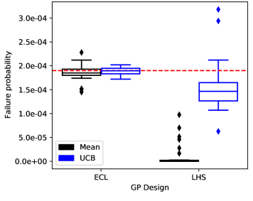
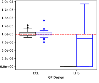
Figure 6: MFIS failure probability estimates $\hat{\alpha}$ for the Ishigami (left) and Hartmann-6 (right) based on GPs trained from ECL adaptive and LHS designs over 30 MC repetitions. The color of each box shows the definition of $\hat{y}(\mathbf{x})$ (black: GP mean; blue: GP 95% upper confidence bound) used to classify failure locations for the bias distribution $\mathbb{F}_{\star}$. The true failure probabilities $\alpha$ are shown with the red-dashed lines.

Just as in Figure 2, using an adaptive design for the GP surrogate $\mathcal{S}$ greatly improves the downstream accuracy of MFIS estimates. Those estimates are centered around the true values (red dashed lines), exemplifying unbiasedness. For the ECL results in Figure 6, using the UCB does not help much, in large part due to the much lower uncertainty around the contour thanks to the contour targeting in adaptive design. Yet in cases where significant uncertainty remains after the adaptive design (LHS results), using UCB may result in a conservative bias distribution over undiscovered sections of the failure region(s).

5.2 Spacesuit impact simulation

NASA’s Artemis program is centered around a renewed effort of manned space exploration. Within this program, NASA is working to develop the next-generation spacesuit, the exploration extravehicular mobility unit (xEMU), to provide astronauts with a suit that is robust, lightweight, and mobile. Under potential impact loads (due to projectiles, falls, etc.) the suit’s probability of no impact failure (PnIF) is of top concern for certification. With the computational model for the xEMU currently under development, we implemented our methodology on a computer model of the previous generation spacesuit, Z-2, to estimate PnIF under various impact loading conditions. The model simulates an impact to the hard upper torso region of the spacesuit (shown in Figure 7) using LS-Dyna finite element method software (Gladman et al., 2007) and the MAT162 material model (Gama et al., 2009; Haque, 2017) to capture the resulting progressive damage to the material.

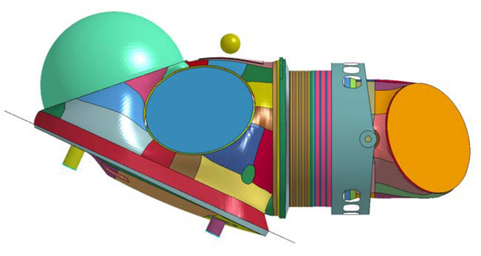
Figure 7: MAT162 assembly model for hard upper torso of Z-2 spacesuit and a rock projectile (yellow sphere).

Based on calibration and sensitivity analysis detailed in Warner et al., (2021), there are four variables in our experiment: three parameters controlling the softening behavior of the material due to damage, henceforth referred to as damage coefficients 1-3, and the impact velocity. The input distribution $\mathbb{F}$ is $\mathbf{x}\sim\mathcal{N}(\bm{\mu},\bm{\Sigma})$ where

$$\bm{\mu}=\begin{bmatrix}0.41597\\ 1.54189\\ 0.01031\\ 1\end{bmatrix}\;\text{and}\;\bm{\Sigma}=\begin{bmatrix}0.00275&-0.00494&-0.00373&0\\ -0.00494&0.01856&0.0032&0\\ -0.00373&0.0032&0.01834&0\\ 0&0&0&0.00016\end{bmatrix}.$$ (11)

The response of interest, $y$, is the maximum contact force, with a threshold of 2800 lbf. Thus to estimate $\alpha=1-\mathrm{PnIF}$, we define $g(y(\mathbf{x}))=y(\mathbf{x})-2800$. The computer model requires 18 hours on 10 cores to produce one sample, severely limiting our ability to entertain a large campaign. We budgeted $N=200$ runs for the adaptive design (including an initial LHS of 40), with adaptive samples generated in batches of ten so the required simulations could be performed in parallel. For the GP surrogate $\mathcal{S}$, we use the Matérn 3/2 (Stein, 2012) kernel with separable lengthscale and a jitter of $10^{-6}$. The data is prescaled to $[0,1]^{4}$ using bounds derived from five standard deviations away from the mean in each dimension.

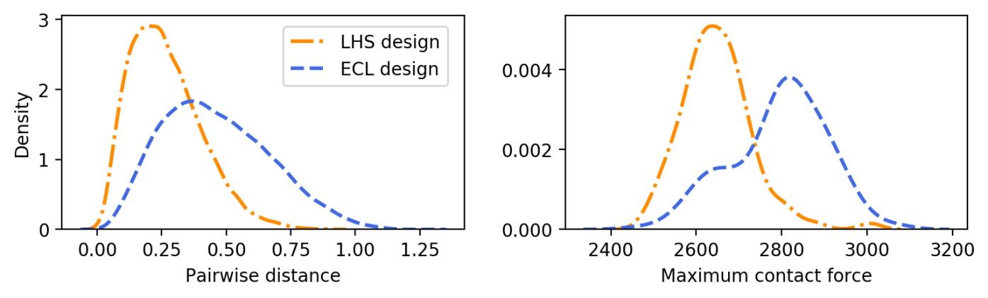
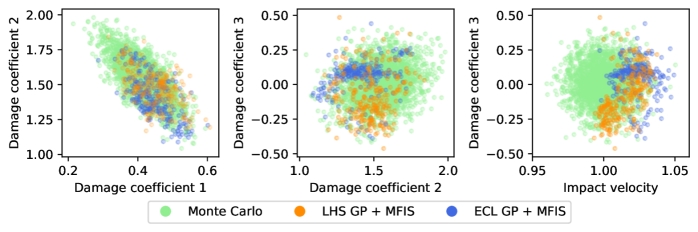
Figure 8: GP designs $(\mathbf{X}_{N},\mathbf{Y}_{N})$ and MFIS samples $\mathbf{X}_{M^{\star}}$ for the Z-2 spacesuit experiment. Top left: pairwise distances for the inputs. Top right: observed outputs from GP designs. Bottom: pairwise plots of samples from input ($\mathbb{F}$, green) and bias ($\mathbb{F}_{\star}$, orange and blue) distributions used for estimating failure probability.

As a benchmarking comparator another GP was fit to a 200-sized LHS that was warped to $\mathbb{F}$ in Eq. (11) via an inverse CDF (dropping the covariances). Figure 8 shows pairwise observed distances in both designs’ set of inputs. The ECL design contains more long distances between points – the inputs are more spread out in the input space. The density in the top right of Figure 8 shows the focus of ECL’s samples around $T=2800$. We take these distinctions as circumstantial evidence that our sequential design method is working.

We used $M=10^{5}$ samples and the $\mathcal{S}$’s UCB to train the bias distribution $\mathbb{F}_{\star}$. Due to the covariances (11) between inputs in $\mathbb{F}$, a Gaussian mixture model with a full covariance structure was used for $\mathbb{F}_{\star}$. We generated $M^{\star}=250$ samples from both bias distributions in order to calculate MFIS estimates. The plots in the bottom of Figure 8 show projections of these samples for select pairs of input variables. While the densities of points look similar for damage coefficient 2 compared to damage coefficient 1, the ECL MFIS samples are biased higher for damage coefficient 3 and impact velocity than compared to LHS MFIS samples. This confirms intuition that higher impact velocity produces more damage, and thus produces failures. As a reference, a set of $M=2500$ pure-MC samples is also shown (generated from $\mathbb{F}$). Both sets of samples from bias distributions show a clear tendency towards sections of the input space targeting predicted failure region(s).

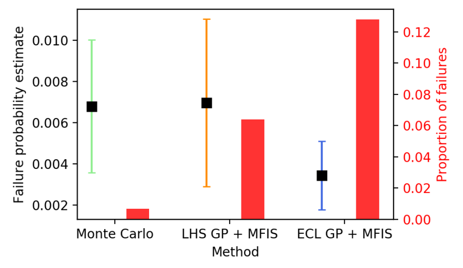
Figure 9: Failure probability estimates $\hat{\alpha}$ with 95% confidence intervals. Red bars show the proportion of samples with failure outputs that were used in those estimates.

MFIS estimates based on the samples in Figure 8 are shown in Figure 9. Notice that the 95% confidence intervals of all three estimates overlap, with the ECL GP $+$ MFIS giving the smallest point estimate. The ECL GP $+$ MFIS estimate also contains the narrowest confidence interval, due to a higher proportion of failures observed in the MFIS samples. The proportion of failures observed in both MFIS estimates may seem low and are no doubt affected by using the GP UCB for classification during $\mathbb{F}_{\star}$ fitting. A higher failure rate for ECL GP $+$ MFIS samples suggests that the bias distribution produced by the UCB of the ECL GP includes the unknown true failure region as a larger proportion of the bias distribution’s density.

6 Discussion

Estimating reliability in engineering applications often entails expensive simulation, limiting the ability to gather large quantities of evaluations. Multifidelity importance sampling is one strategy to reduce the amount of data needed for an unbiased reliability estimate, leveraging a surrogate model (like a GP) and bias distribution to reduce estimator variance. If the GP’s predictive surface is inaccurate in the vicinity of the true failure contour, misclassified samples may be used to fit a bias distribution, threatening the overall accuracy of the reliability estimate. By marrying a GP built on an adaptive design for contour location with MFIS, we can guard against such pitfalls.

We proposed a thrifty adaptive design with a novel criteria: the Entropy-based Contour Locator (ECL). Our ECL acquisition function applies the basic definition of entropy on events derived from predicted pass/fail from the surrogate. Everything for ECL has a closed form. We solve for a new acquisition, maximizing ECL, in such a way that multiple failure regions based on high quantiles may be identified. Results showed that our ECL adaptive designs exhibited a degree of stochasticity in optimization that promoted exploration of local maxima. When problems contain multiple failure regions, especially ones with small relative volumes, this exploration is key. Our examples include illustrative benchmarks with two (2d and 6d) and six (3d) failure regions. Against a litany of contemporary adaptive design benchmarks, ECL performs among the best at correctly identifying true failures as well as estimating the contour’s volume. All this is accomplished at a one to two orders of magnitude computational savings. We also implemented ECL design plus MFIS on spacesuit damage simulator, demonstrating how combining these two methods provides a point estimate with less uncertainty than plain MC or MFIS techniques.

We demonstrated how the adaptive design process with ECL may be extended to batch selection, providing computational savings when parallel-processing is available. By selecting multiple points before observing more responses, the batch option is more sensitive to the quality of surrogate, and in particular its contour estimate(s). Batch size also plays a role in the quality of the information gained from the sample points. In high-dimensional problems, batch selection is crucial for the method to be tractable. While we fixed the batch size for our experiments, the method could likely be improved by setting the batch size as a function of available computing time.

Our methodological contribution focused on targeting failure regions with ECL, not explicitly on its interface with MFIS. Rather, we treated MFIS as one, of possibly several, downstream reliability tasks after ECL acquisition. This compartmental nature is an asset, as it means our contribution is portable. However, it also means potential for improved efficiency in the reliability context was left on the table. We believe there is opportunity for further blending of adaptive design and MFIS: perhaps by generating acquisitions and refining MFIS bias distributions $\mathbb{F}_{\star}$ at the same time.

Appendix A Value of integration knot density

When applying any of the adaptive designs in Section 4.2, there are certain choices, or “knobs”, that play a crucial role in optimizing the acquisition function. Though both CLoVER and ECL use entropy in their acquisition functions, performing adaptive design with CLoVER includes two knobs, whereas ECL only has one. Here we explore the effect of different knob settings for experiments detailed in Section 4.

To begin, we focus on the strategy used to optimize the acquisition function. ECL uses Algorithm 2, which contains a small set of $N_{c}=10d$ candidate points and a continuous optimization initialized at the best candidate. For CLoVER, Marques et al., (2018) propose candidates only, forgoing a continuous optimizer. In their code, they use a single candidate set from which to select all new design locations. For our experiments, we fix that set to be an LHS of 1000 points. The results shown in Section 4.2 use these strategies. In Figure 10, we supplement that experiment with swapped optimization strategies for ECL and CLoVER. ECL’s original strategy is denoted with solid lines and triangles and CLoVER’s single candidate set strategy is shown with the dashed lines and squares. CLoVER and ECL follow a similar trajectory for sensitivity and relative error when a single candidate set is used. With Algorithm 2, CLoVER’s sensitivity lags behind ECL during the first half of the experiment.

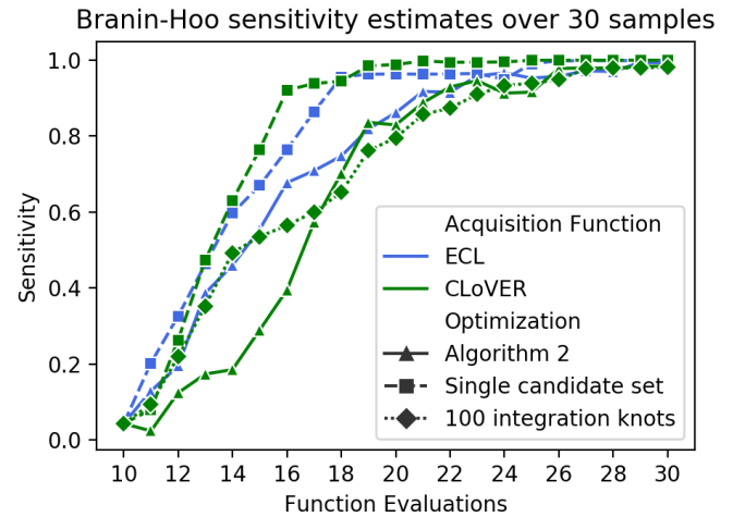
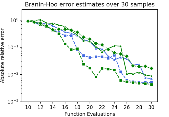
Figure 10: Mean sensitivity (left) and relative error of the volume estimate (right) for the Branin-Hoo experiment over 30 MC repetitions. The ECL (blue) and CLoVER (green) acquisition functions are used with different optimization strategies.

In the Ishigami experiment, we find a more complex story (Figure 11). Here we provide the sensitivity and absolute relative error distributions for the 30 repetitions at the experiment’s conclusion. Since the number of sequential samples (170) is a large proportion of the candidate set’s size, we introduce a third optimization strategy that generates unique 1000-sized LHSs at each adaptive step (blue boxes). For ECL, using Algorithm 2 for optimization (purple box) clearly beats both a single candidate set (yellow box) or unique candidate sets for each iteration.

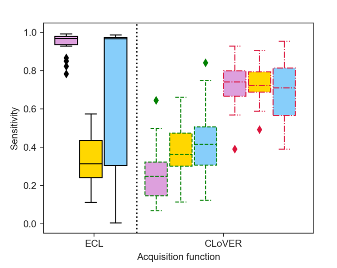
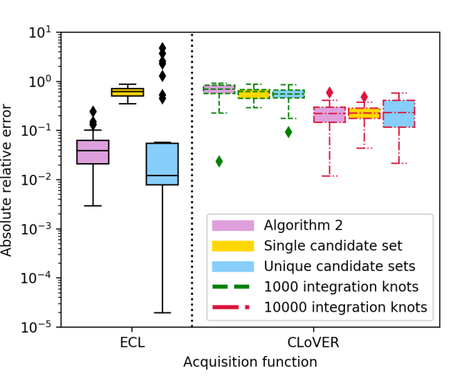
Figure 11: Final sensitivity (left) and relative error (right) for the Ishigami experiment. Different optimization strategies are used on the ECL and/or CLoVER acquisition functions, changing the number of candidate points and integration knots.

Unlike with ECL, the CLoVER results in Figure 11 do not show a drastic change in sensitivity or relative error across optimization strategies. With the Ishigami experiment being harder (larger quantile, more failure regions) than Branin-Hoo, the original set of 1000 integration knots may be too small. Increasing to 10000 knots shows a significant improvement for all optimization strategies. Looking back at the Branin-Hoo experiment in Figure 10, we added a CLoVER variation using a single candidate set and only 100 integration points (dotted line with triangles). We find the sensitivity is below CLoVER with 1000 knots for a majority of the experiment and the relative error is significantly higher.

Optimization Strategy	ECL	CLoVER
		$10^{3}$ knots	$10^{4}$ knots
Algorithm 2	0.008	15.2	17.1
Single candidate set	0.09	17.8	32.4
Unique candidate sets	0.14	18.2	28.7

Table 3: Average computation times (minutes) to select points across 30 MC repetitions of the Ishigami experiment.

Increasing the number of optimization candidate points or integration knots comes at a price – namely computation time. Table 3 summarizes the drastic difference in computing times between ECL and CLoVER for the Ishigami experiment. For challenging problems like Ishigami, an even greater number of integration knots seems necessary to produce competitively accurate results. When accounting for the additional computational burden, implementing CLoVER with a large number of knots in higher dimensional problems (i.e. Hartmann-6) could be impractical based on current software.

References

- Au and Beck, (2001) Au, S.-K. and Beck, J. L. (2001). “Estimation of small failure probabilities in high dimensions by subset simulation.” Probabilistic Engineering Mechanics, 16, 4, 263–277.
- Auffray et al., (2014) Auffray, Y., Barbillon, P., and Marin, J.-M. (2014). “Bounding rare event probabilities in computer experiments.” Computational Statistics & Data Analysis, 80, 153–166.
- Azzimonti et al., (2016) Azzimonti, D., Bect, J., Chevalier, C., and Ginsbourger, D. (2016). “Quantifying uncertainties on excursion sets under a Gaussian random field prior.” SIAM/ASA Journal on Uncertainty Quantification, 4, 1, 850–874.
- Azzimonti et al., (2020) Azzimonti, D., Ginsbourger, D., Chevalier, C., Bect, J., and Richet, Y. (2020). “Adaptive design of experiments for conservative estimation of excursion sets.” Technometrics, 1–14.
- Barnett, (1979) Barnett, S. (1979). Matrix Methods for Engineers and Scientists. McGraw-Hill.
- Bect et al., (2012) Bect, J., Ginsbourger, D., Li, L., Picheny, V., and Vazquez, E. (2012). “Sequential design of computer experiments for the estimation of a probability of failure.” Statistics and Computing, 22, 3, 773–793.
- Bichon et al., (2008) Bichon, B. J., Eldred, M. S., Swiler, L. P., Mahadevan, S., and McFarland, J. M. (2008). “Efficient global reliability analysis for nonlinear implicit performance functions.” AIAA Journal, 46, 10, 2459–2468.
- Bogunovic et al., (2016) Bogunovic, I., Scarlett, J., Krause, A., and Cevher, V. (2016). “Truncated variance reduction: a unified approach to Bayesian optimization and level-set estimation.” In Advances in Neural Information Processing Systems, eds. D. Lee, M. Sugiyama, U. Luxburg, I. Guyon, and R. Garnett, vol. 29, 1507–1515. Curran Associates, Inc.
- Bolin and Lindgren, (2015) Bolin, D. and Lindgren, F. (2015). “Excursion and contour uncertainty regions for latent Gaussian models.” Journal of the Royal Statistical Society: Series B: Statistical Methodology, 85–106.
- Bryan and Schneider, (2008) Bryan, B. and Schneider, J. (2008). “Actively learning level-sets of composite functions.” In Proceedings of the 25th International Conference on Machine Learning, 80–87.
- Byrd et al., (1995) Byrd, R., Qiu, P., Nocedal, J., , and Zhu, C. (1995). “A limited memory algorithm for bound constrained optimization.” Journal on Scientific Computing, 16, 5, 1190–1208.
- Cannamela et al., (2008) Cannamela, C., Garnier, J., Iooss, B., et al. (2008). “Controlled stratification for quantile estimation.” The Annals of Applied Statistics, 2, 4, 1554–1580.
- Celeux and Govaert, (1995) Celeux, G. and Govaert, G. (1995). “Gaussian parsimonious clustering models.” Pattern Recognition, 28, 5, 781–793.
- Chevalier et al., (2014) Chevalier, C., Bect, J., Ginsbourger, D., Vazquez, E., Picheny, V., and Richet, Y. (2014). “Fast parallel kriging-based stepwise uncertainty reduction with application to the identification of an excursion set.” Technometrics, 56, 4, 455–465.
- Chevalier et al., (2013) Chevalier, C., Ginsbourger, D., Bect, J., and Molchanov, I. (2013). “Estimating and quantifying uncertainties on level sets using the Vorob’ev expectation and deviation with Gaussian process models.” In MODA 10–Advances in Model-Oriented Design and Analysis, 35–43. Springer.
- Cliffe et al., (2011) Cliffe, K. A., Giles, M. B., Scheichl, R., and Teckentrup, A. L. (2011). “Multilevel Monte Carlo methods and applications to elliptic PDEs with random coefficients.” Computing and Visualization in Science, 14, 1, 3.
- Cohn, (1994) Cohn, D. A. (1994). “Neural network exploration using optimal experiment design.” In Advances in Neural Information Processing Systems 6, eds. J. D. Cowan, G. Tesauro, and J. Alspector, 679–686. Morgan-Kaufmann.
- Cover, (2006) Cover, T. M. (2006). Elements of information theory. John Wiley & Sons.
- Dubourg and Deheeger, (2011) Dubourg, V. and Deheeger, F. (2011). “Metamodel-based importance sampling for the simulation.” Applications of Statistics and Probability in Civil Engineering, 26, 192.
- Echard et al., (2010) Echard, B., Gayton, N., and Lemaire, M. (2010). “Kriging-based monte carlo simulation to compute the probability of failure efficiently: AK-MCS method.” 6èmes Journées Nationales de Fiabilité.
- Fernández-Godino et al., (2016) Fernández-Godino, M. G., Park, C., Kim, N.-H., and Haftka, R. T. (2016). “Review of multi-fidelity models.” arXiv preprint arXiv:1609.07196.
- Fernández-Godino et al., (2019) Fernández-Godino, M. G., Park, C., Kim, N. H., and Haftka, R. T. (2019). “Issues in deciding whether to use multifidelity surrogates.” AIAA Journal, 57, 5, 2039–2054.
- Forrester et al., (2008) Forrester, A., Sobester, A., and Keane, A. (2008). Engineering design via surrogate modelling: a practical guide. John Wiley & Sons.
- Gama et al., (2009) Gama, B. A., Bogetti, T. A., and Gillespie Jr, J. W. (2009). “Progressive damage modeling of plain-weave composites using LS-Dyna composite damage model MAT162.” In 7th European LS-DYNA Conference, 14–15.
- Genz and Bretz, (2009) Genz, A. and Bretz, F. (2009). Computation of multivariate normal and t probabilities, vol. 195. Springer Science & Business Media.
- Genz et al., (2019) Genz, A., Bretz, F., Miwa, T., Mi, X., Leisch, F., Scheipl, F., and Hothorn, T. (2019). mvtnorm: multivariate normal and distributions. R package version 1.0-10.
- Giles, (2008) Giles, M. B. (2008). “Multilevel monte carlo path simulation.” Operations Research, 56, 3, 607–617.
- Gladman et al., (2007) Gladman, B. et al. (2007). LS-DYNA keyword users’ manual (Version 971). Livermore Software Technology Corporation.
- Gotovos, (2013) Gotovos, A. (2013). “Active learning for level set estimation.” Master’s thesis, Eidgenössische Technische Hochschule Zürich, Department of Computer Science.
- Gramacy, (2011) Gramacy, R. (2011). ““Optimization under unknown constraints,” in Proceedings of the Ninth Valencia International Meetings on Bayesian Statistics.”
- Gramacy and Polson, (2011) Gramacy, R. and Polson, N. (2011). “Particle learning of Gaussian process models for sequential design and optimization.” Journal of Computational and Graphical Statistics, 20, 1, 102–118.
- Gramacy, (2020) Gramacy, R. B. (2020). Surrogates: Gaussian process modeling, design and optimization for the applied sciences. Boca Raton, Florida: Chapman Hall/CRC. http://bobby.gramacy.com/surrogates/.
- Gramacy and Apley, (2015) Gramacy, R. B. and Apley, D. W. (2015). “Local Gaussian process approximation for large computer experiments.” Journal of Computational and Graphical Statistics, 24, 2, 561–578.
- Haque, (2017) Haque, B. Z. G. (2017). “A progressive composite damage model for unidirectional and woven fabric composites.” Materials Science Corporation (MSC) and University of Delaware Center for Composite Materials (UD-CCM).
- Ishigami and Homma, (1990) Ishigami, T. and Homma, T. (1990). “An importance quantification technique in uncertainty analysis for computer models.” In [1990] Proceedings. First International Symposium on Uncertainty Modeling and Analysis, 398–403. IEEE.
- Jones et al., (1998) Jones, D. R., Schonlau, M., and Welch, W. J. (1998). “Efficient global optimization of expensive black-box functions.” Journal of Global Optimization, 13, 4, 455–492.
- Lee and Jung, (2008) Lee, T. and Jung, J. (2008). “A sampling technique enhancing accuracy and efficiency of metamodel-based RBDO: Constraint boundary sampling.” Computers & Structures, 86, 13, 1463 – 1476. Structural Optimization.
- Li et al., (2011) Li, J., Li, J., and Xiu, D. (2011). “An efficient surrogate-based method for computing rare failure probability.” Journal of Computational Physics, 230, 24, 8683–8697.
- Li and Xiu, (2010) Li, J. and Xiu, D. (2010). “Evaluation of failure probability via surrogate models.” Journal of Computational Physics, 229, 23, 8966–8980.
- Litvinenko et al., (2013) Litvinenko, A., Matthies, H. G., and El-Moselhy, T. A. (2013). “Sampling and low-rank tensor approximation of the response surface.” In Monte Carlo and Quasi-Monte Carlo Methods, 535–551. Springer.
- Loeppky et al., (2009) Loeppky, J. L., Sacks, J., and Welch, W. J. (2009). “Choosing the sample size of a computer experiment: a practical guide.” Technometrics, 51, 4.
- Lyu et al., (2021) Lyu, X., Binois, M., and Ludkovski, M. (2021). “Evaluating Gaussian process metamodels and sequential designs for noisy level set estimation.” Statistics and Computing, 31, 4, 1–21.
- MacKay, (1992) MacKay, D. J. (1992). “Information-based objective functions for active data selection.” Neural Computation, 4, 4, 590–604.
- Marques et al., (2018) Marques, A., Lam, R., and Willcox, K. (2018). “Contour location via entropy reduction leveraging multiple information sources.” In Advances in Neural Information Processing Systems, 5217–5227.
- Mckay et al., (1979) Mckay, M., Beckman, R., and Conover, W. (1979). “A comparison of three methods for selecting values of input variables in the analysis of output from a computer code.” Technometrics, 21, 239–245.
- Melchers and Beck, (2018) Melchers, R. E. and Beck, A. T. (2018). Structural Reliability Analysis and Prediction. John wiley & sons.
- Neal, (1998) Neal, R. M. (1998). “Regression and classification using Gaussian process priors.” Bayesian Statistics, 6, 475–501.
- Oakley, (2004) Oakley, J. (2004). “Estimating percentiles of uncertain computer code outputs.” Journal of the Royal Statistical Society: Series C (Applied Statistics), 53, 1, 83–93.
- Pedregosa et al., (2011) Pedregosa, F., Varoquaux, G., Gramfort, A., Michel, V., Thirion, B., Grisel, O., Blondel, M., Prettenhofer, P., Weiss, R., Dubourg, V., Vanderplas, J., Passos, A., Cournapeau, D., Brucher, M., Perrot, M., and Duchesnay, E. (2011). “Scikit-learn: machine learning in Python.” Journal of Machine Learning Research, 12, 2825–2830.
- Peherstorfer et al., (2016) Peherstorfer, B., Cui, T., Marzouk, Y., and Willcox, K. (2016). “Multifidelity importance sampling.” Computer Methods in Applied Mechanics and Engineering, 300, 490–509.
- Peherstorfer et al., (2018a) Peherstorfer, B., Kramer, B., and Willcox, K. (2018a). “Multifidelity preconditioning of the cross-entropy method for rare event simulation and failure probability estimation.” SIAM/ASA Journal on Uncertainty Quantification, 6, 2, 737–761.
- Peherstorfer et al., (2018b) Peherstorfer, B., Willcox, K., and Gunzburger, M. (2018b). “Survey of multifidelity methods in uncertainty propagation, inference, and optimization.” SIAM Review, 60, 3, 550–591.
- Picheny et al., (2010) Picheny, V., Ginsbourger, D., Roustant, O., Haftka, R. T., and Kim, N.-H. (2010). “Adaptive designs of experiments for accurate approximation of a target region.” Journal of Mechanical Design, 132, 7.
- R Core Team, (2021) R Core Team (2021). R: a language and environment for statistical computing. R Foundation for Statistical Computing, Vienna, Austria.
- Ranjan et al., (2008) Ranjan, P., Bingham, D., and Michailidis, G. (2008). “Sequential experiment design for contour estimation from complex computer codes.” Technometrics, 50, 4, 527–541.
- Robert and Casella, (2013) Robert, C. and Casella, G. (2013). Monte Carlo statistical methods. Springer Science & Business Media.
- Roustant et al., (2012) Roustant, O., Ginsbourger, D., and Deville, Y. (2012). “DiceKriging, DiceOptim: two R packages for the analysis of computer experiments by kriging-based metamodeling and optimization.” Journal of Statistical Software, 51, 1, 1–55.
- Sacks et al., (1989) Sacks, J., Welch, W., J. Mitchell, T., and Wynn, H. (1989). “Design and analysis of computer experiments. With comments and a rejoinder by the authors.” Statistical Science, 4.
- Santner et al., (2018) Santner, T., Williams, B., and Notz, W. (2018). The design and analysis computer experiments. Springer; 2nd edition.
- Seo et al., (2000) Seo, S., Wallat, M., Graepel, T., and Obermayer, K. (2000). “Gaussian process regression: Active data selection and test point rejection.” In Mustererkennung 2000, 27–34. Springer.
- Settles, (2011) Settles, B. (2011). “From theories to queries: active learning in practice.” In Active Learning and Experimental Design Workshop In Conjunction With AISTATS 2010, 1–18.
- Srinivasan, (2013) Srinivasan, R. (2013). Importance sampling: applications in communications and detection. Springer Science & Business Media.
- Stein, (2012) Stein, M. L. (2012). Interpolation of spatial data: some theory for kriging. Springer Series in Statistics. Springer New York.
- Surjanovic and Bingham, (2014) Surjanovic, S. and Bingham, D. (2014). “Virtual library of simulation experiments: test functions and datasets–optimization test problems (sum of different powers function). sfu. ca/~ ssurjano/index. html.” Or just google sum of different powers function.
- Warner et al., (2021) Warner, J., Leser, P., Leser, W., Cole, D. A., and Bomarito, G. (2021). “Assessing next-gen spacesuit reliatibilty: a probabilistic analysis case study.” Tech. rep.
- Wolpert and Macready, (1997) Wolpert, D. H. and Macready, W. G. (1997). “No free lunch theorems for optimization.” IEEE Transactions on Evolutionary Computation, 1, 1, 67–82.
- Wu et al., (2017) Wu, J., Poloczek, M., Wilson, A. G., and Frazier, P. (2017). “Bayesian optimization with gradients.” In Advances in Neural Information Processing Systems, 5267–5278.
- Zhang et al., (2021) Zhang, B., Cole, D. A., and Gramacy, R. B. (2021). “Distance-distributed design for Gaussian process surrogates.” Technometrics, 63, 1, 40–52.
- Zhang et al., (2020) Zhang, B., Gramacy, R. B., Johnson, L., Rose, K. A., and Smith, E. (2020). “Batch-sequential design and heteroskedastic surrogate modeling for delta smelt conservation.” arXiv preprint arXiv:2010.06515.