Brain tumour segmentation using a triplanar ensemble of U-Nets on MR images

Abstract

Gliomas appear with wide variation in their characteristics both in terms of their appearance and location on brain MR images, which makes robust tumour segmentation highly challenging, and leads to high inter-rater variability even in manual segmentations. In this work, we propose a triplanar ensemble network, with an independent tumour core prediction module, for accurate segmentation of these tumours and their sub-regions. On evaluating our method on the MICCAI Brain Tumor Segmentation (BraTS) challenge validation dataset, for tumour sub-regions, we achieved a Dice similarity coefficient of 0.77 for both enhancing tumour (ET) and tumour core (TC). In the case of the whole tumour (WT) region, we achieved a Dice value of 0.89, which is on par with the top-ranking methods from BraTS’17-19. Our method achieved an evaluation score that was the equal 5^th highest value (with our method ranking in 10^th place) in the BraTS’20 challenge, with mean Dice values of 0.81, 0.89 and 0.84 on ET, WT and TC regions respectively on the BraTS’20 unseen test dataset.

1 Introduction

Gliomas, the most common class of brain tumours, occur with different levels of aggressiveness with highly heterogeneous sub-regions including invaded edematous tissue or peritumoral edema (ED) and tumour core region including necrotic core (NCR), non-enhancing tumour (NET), and enhancing tumour (ET) [1], [2]. Accurate and reproducible automated detection of gliomas would aid in the timely diagnosis and staging of tumours in a clinical setting, and reliable analysis in large population studies. However, the intrinsic histological variations of gliomas are further complicated by the heterogeneity in characteristics (e.g. intensity) of tumours on MRI scans. Various sub-regions of gliomas occur with wide variations in their appearance and shape depending on their biological conditions, making their segmentation highly challenging and often leading to high inter-rater variability even in expert clinicians’ segmentations across different datasets [1].

The MICCAI Brain Tumor Segmentation (BraTS) challenges aim to provide accurate segmentation of brain tumours on multimodal MR images [1], [2], [3], [4], [5]. Several methods, including recent deep learning methods, have been proposed in BraTS challenges. The top ranking methods used convolutional neural network (CNN) architectures [6], [7], [8], [9] mostly using ensemble networks [10], [11], [12] and/or encoder-decoder frameworks [13], [14]. U-Nets [15], one of the most popular encoder-decoder networks, were used successfully with accurate results for tumour segmentation [16], [17], [18], [19]. Regarding the model dimensions, both 2D [6] and 3D networks [7] were used with additional post-processing steps (e.g. conditional random fields used in [7], [9]) and occasionally within multi-scale architectures [7], [8] and multi-step cascaded frameworks [12], [19]. Some methods aimed to leverage the advantages of both 2D and 3D architecture by using triplanar ensembles of CNNs [12], providing accurate segmentation with fewer parameters than 3D networks. Further, modifications to the loss functions have been proposed [9], [12] for overcoming class imbalance, reliable tumour core detection and accurate segmentation of tumour boundaries.

We propose a fully automated deep learning method for brain tumour segmentation using a triplanar ensemble architecture consisting of a 2D U-Net in each plane (axial, sagittal and coronal) of MR images. Our method uses a combination of loss functions in order to overcome the class imbalance and includes an independent tumour core prediction module to refine the segmentation of tumour core sub-regions. We study the effect of various components of our architecture on the segmentation results by performing an ablation study. We evaluate our method on BraTS’20 training and validation datasets, which exhibit wide heterogeneity in tumour characteristics and provides a benchmark to assess the robustness of our segmentation method. Finally, the results of our method on BraTS’20 test dataset shows that our method provides accurate segmentation of tumour regions, ranking among the top 10 best performing methods of the challenge.

2 Materials and methods

2.1 Data

We evaluated the performance of the proposed method on the publicly available BraTS’20 dataset, consisting of pre-operative multimodal MRI scans, with 369 training cases. For each subject, the given input modalities include FLAIR, T1-weighted (T1), post-contrast T1-weighted (T1-CE) and T2-weighted (T2) images. The manual segmentations for the training dataset consists of 3 labels [1], [2]: NCR/NET, ED and ET. The input modalities (FLAIR, T1, T1-CE, T2) were already co-registered to the same anatomical template of dimension 240 $\times$ 240 $\times$ 155, interpolated to the same resolution (1 mm³ isotropic) and skull-stripped. In addition to the training data, 125 validation cases were provided without manual segmentations (referred from now on as “unlabelled validation dataset”) to enable an initial validation of the method via the challenge’s online evaluation platform (using the ground truth at their end). Additionally, 166 test cases without manual segmentations (referred from now on as “unseen test dataset”) were released for a duration of 48 hours for the final testing via the online evaluation platform (again, using their local ground truth).

2.2 Preprocessing

We cropped the images to a standard size of 192 $\times$ 192 $\times$ 160 voxels so that field of view (FOV) is close to the brain, and applied Gaussian normalisation to the intensity values. We then extracted 2D slices from the volumes from axial, sagittal and coronal planes with dimensions of 192 $\times$ 192, 192 $\times$ 160 and 192 $\times$ 160 voxels respectively.

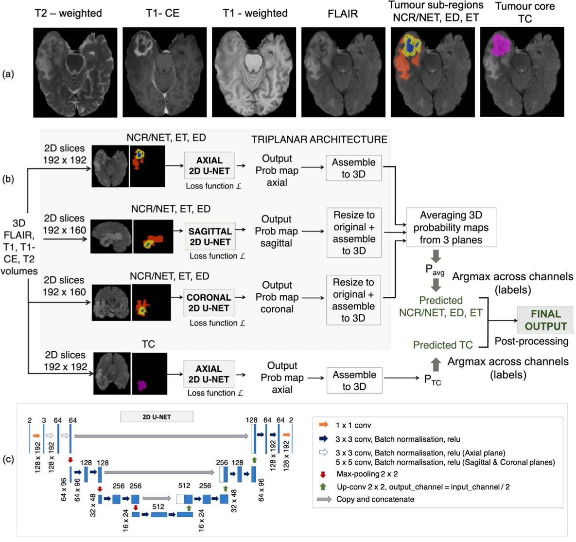
Figure 1: Proposed triplanar ensemble network architecture. (a) Input modalities in the axial plane along with manual segmentations for NCR/NET (blue), ET (yellow), ED (red) and TC (magenta), (b) the proposed network and (c) 3-layer deep U-Net blocks used in (b). Slices with 4 channels (input modalities) were provided to all U-nets.

2.3 CNN architecture

We used the triplanar architecture proposed in [20]. Briefly, as shown in fig. 1, the triplanar architecture consists of three 2D U-Nets, one for each plane, taking FLAIR, T1, T1-CE and T2 slices as input channels. On the training dataset, we observed that while the manual segmentation for the cumulative tumour core (TC, which is ET + NCR/NET) (fig. 1a) was quite consistent, there were wide variations in those of individual sub-regions (NCR/NET and ET), due to their underlying histological heterogeneity. Therefore, in order to reduce the inconsistencies in the boundaries of ET and NCR/NET labels, we modified the ground truth labels to include TC in addition to the provided labels, obtaining 4 labels: ET, ED, NCR/NET and TC. During training, we used the ET, NCR/NET and ED labels to train the U-Nets in the triplanar architecture, while we used the TC label to train an independent axial U-Net as shown in fig. 1b. We later used the TC regions in the post-processing step (refer section 2.4) to further refine the final output labels (ET, NCR/NET and ED).

We trimmed the depth of the classic U-Net [15] in each plane to a depth of 3-layers (fig. 1b), to reduce the computational load. While axial U-Nets use 3 $\times$ 3 convolutional kernels in the initial layer, the other two U-Nets use 5 $\times$ 5 kernels. This helped to learn more generic lesion patterns, thus avoiding any discontinuities in segmentation along the z-dimension. In the ensemble model, we trained the U-Nets in each plane independently using 2D slices extracted in each plane. We used a combination of cross-entropy (CE) and Dice loss (DL) functions in order to overcome the effect of class imbalance between tumour/edema and healthy tissue. The loss function was computed batch-wise as shown below in eqn 1.

$$L=CE+DL=-\sum\limits_{c=1}^{C}y_{c}(x)\text{log}(p_{c}(x))-\frac{1}{C}\sum\limits_{c=1}^{C}\frac{2\times\sum_{x=1}^{N}M_{c}(x)\cdot PL_{c}(x)}{\sum_{x=1}^{N}M_{c}(x)+\sum_{x=1}^{N}PL_{c}(x)}$$ (1)

where $p_{c}(x)$ denotes the output of the soft-max layer, $C$ is the number of classes in labels, $y_{c}(x)\in\{0,1\}$ indicates the binary value at voxel $x$ for each class, $M_{c}$ indicates the manual segmentation and $PL_{c}$ indicates the predicted label map obtained by determining the argmax of labels from the soft-max output.

During testing, the predictions were obtained as 2D probability maps for slices in each plane and were later assembled into 3D volumes and resized to the original dimensions. We then averaged the 3D probability volumes to get the final probability volume ($P_{avg}$) for the triplanar architecture. In addition, we obtained a 3D probability map ($P_{TC}$) from the independent axial U-Net for predicting TC label. Note that 3D probability maps $P_{avg}$ and $P_{TC}$ still have a 4${}^{\text{th}}$ dimension corresponding to the labels.

2.4 Post-processing

We obtained the predicted ET, NCR/NET and ED label maps by determining the argmax of labels (4${}^{\text{th}}$ dimension) in $P_{avg}$ and padded them with zeros to bring them back to their original dimensions. Similarly, we obtained the predicted the TC label map from $P_{TC}$ as argmax of TC against background. We then applied the following additional rules, based on prior knowledge and patterns observed in the manual segmentations: predicted ET regions with volume $<$ 200 mm³ were relabeled as part of the NCR/NET region; the difference between TC and ET was relabelled as NCR/NET. We also performed a morphological clean-up by removing small isolated noisy stray regions in ED output (volume $<$ 200 mm³ and located at a distance $>$ 75 mm from the centre of the largest ED region) and filled in the missed voxels in the TC - ED interfaces as part of the ED output.

2.5 Implementation details

The models were trained using the Adam Optimiser with $\epsilon$=$10^{-4}$. We empirically chose a batch size of 8, with an initial learning rate of $1\times 10^{-3}$, reducing it by a factor of $1\times 10^{-1}$ every 2 epochs (set empirically due to the rapid reduction of loss values at these early epochs), until it reached a fixed value of $1\times 10^{-5}$. Every individual U-Net took $\approx$ 50 epochs for convergence. The networks were trained on an NVIDIA Tesla V100, taking $\approx$ 12 mins (for 3 planes + TC network) per epoch training/validation split of 90%/10%.

2.6 Data augmentation

Data augmentation was applied in an online manner by randomly selecting from following transformations: translation (x/y-offset $\in$ [-10, 10]), rotation ($\theta$ $\in$ [-10, 10]) and random noise injection (Gaussian, $\mu$ = 0, $\sigma^{2}$ $\in$ [0.01, 0.09]), increasing the dataset by a factor of 2 (chosen empirically) for all planes. The hyperparameters for the transformations were randomly sampled from the above specified closed intervals using a uniform distribution.

2.7 Performance evaluation metrics

Metrics computed by the online evaluation platform in BraTS’20 are (i) Dice Similarity Coefficient measured as 2 $\times$ TP / (2 $\times$ TP + FP + FN), (ii) sensitivity measured as TP / (TP + FN), (iii) specificity measured as TN / (TN + FP) and (iv) the 95${}^{\text{th}}$ percentile of the Hausdorff Distance (H95), where TP, FP, FN and TN are number of true positive, false positive, false negative and true negative voxels respectively. Regarding the ground truth labels, while the manual segmentations consist of ET, ED and NCR/NET classes, evaluation performance metrics were determined by the evaluation platform for the following sub-regions of tumour: (1) ET, (2) TC (NCR/NET + ET) and (3) whole tumour (WT, which is TC + ED).

3 Experiments and results

Cross-validation on the labelled training data: We used 369 labelled subjects from BraTS’20 training data to perform 5-fold cross-validation with a training-validation-testing split ratio of 255-37-73 subjects (255-37-77 for the last fold). The results on the test splits (evaluated using the challenge online platform) are shown in table 1. Among the three sub-regions, we achieved the best segmentation performance for the whole tumour (WT) with a mean Dice value of 0.93. A few sample outputs of our method are shown along with manual segmentations in fig. 2.

Table 1: Results of 5-fold cross-validation on BraTS’20 Training data.

	Dice			Sensitivity			Specificity			H95 (mm)
	ET	WT	TC	ET	WT	TC	ET	WT	TC	ET	WT	TC
Mean	0.83	0.93	0.87	0.83	0.90	0.85	0.99	0.99	0.99	20.3	3.4	6.3
Std.	0.22	0.08	0.17	0.23	0.11	0.19	.0005	.0005	.0005	80.3	5.1	28.0
Median	0.90	0.95	0.93	0.91	0.93	0.93	0.99	0.99	0.99	1.0	1.7	2.2
25 quantile	0.83	0.91	0.86	0.83	0.87	0.83	0.99	0.99	0.99	1.0	1.0	1.4
75 quantile	0.95	0.97	0.96	0.96	0.97	0.97	0.99	0.99	0.99	2.2	3.2	4.2
ET - enhancing tumour, WT - whole tumour, TC - tumour core.

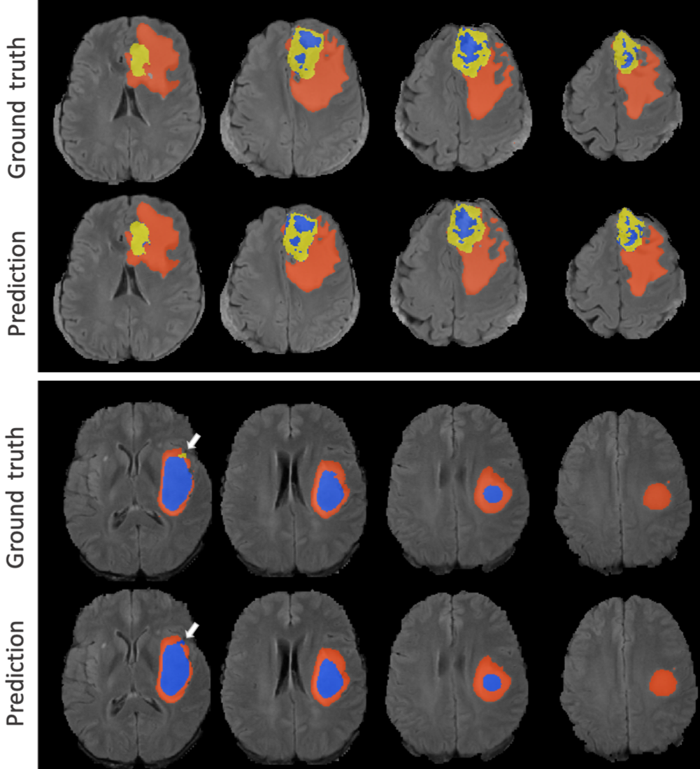
Figure 2: Results on BraTS’20 training data from two sample subjects (top and bottom panels). Manual segmentations and predicted outputs on axial slices from two sample subjects (NCR/NET - blue, ET - yellow and ED - red). Subject in the top panel: Dice (ET/WT/TC) - 0.96/0.98/0.97, sensitivity (ET/WT/TC) - 0.95/0.98/0.99, specificity (all) - 0.99, H95 (all) - 1 mm; subject in the bottom panel: Dice (ET/WT/TC) - 0/0.98/0.94, sensitivity (ET/WT/TC) - 0/0.97/0.89, specificity (ET/WT/TC) - 1/0.99/1, H95 (ET/WT/TC) - 373.1/1/1.4. In the bottom panel, the white arrows indicate the false prediction of the ET region, leading to the dice value of 0.00.

Ablation study on the labelled training data: In order to determine the effect of individual components of our architecture on the segmentation performance, we evaluated the segmentation results with the following components: (i) axial 2D U-Net only, (ii) axial + sagittal 2D U-Nets, (iii) triplanar network (axial + sagittal + coronal U-Nets) and (iv) triplanar network + axial U-Net for TC label detection. We used a cross-validation strategy (with the same training-validation-test split mentioned above) to evaluate the performance metrics. The values of performance metrics for the ablation study are shown in table 2 and the corresponding boxplots are shown in fig. 3. The segmentation of sub-regions improved with the addition of the TC network, with significant increase in Dice and sensitivity values (p $<$ 0.01), especially for the ET and TC sub-regions. We also observed significant improvement in the specificity of the WT segmentation (p $<$ 0.001) using the triplanar architecture when compared to individual U-Nets.

Table 2: Ablation study results for BraTS’20 Training data. Mean and standard deviation (in brackets) values for various components of the method reported for tumour sub-regions. In the lower part p-values of paired two-tailed t-test results between individual pairs of components are shown, with significant values underlined.

	Dice			Sensitivity			Specificity			H95 (mm)
	ET	WT	TC	ET	WT	TC	ET	WT	TC	ET	WT	TC
A	0.78 (0.25)	0.89 (0.10)	0.80 (0.24)	0.78 (0.26)	0.86 (0.13)	0.76 (0.26)	0.9997 (.0006)	0.9994 (.0007)	0.9997 (.0005)	26.6 (89.7)	5.7 (7.9)	7.3 (20.9)
A+S	0.79 (0.24)	0.90 (0.10)	0.82 (0.21)	0.79 (0.26)	0.87 (0.13)	0.83 (0.23)	0.9997 (.0006)	0.9995 (.0006)	0.9995 (.0008)	25.9 (89.7)	4.9 (8.4)	7.4 (21.4)
TP	0.79 (0.24)	0.90 (0.09)	0.83 (0.21)	0.79 (0.26)	0.86 (0.14)	0.82 (0.23)	0.9997 (.0006)	0.9996 (.0006)	0.9997 (.0006)	25.8 (89.6)	4.6 (6.1)	7.0 (28.0)
TP+TC	0.82 (0.22)	0.92 (0.07)	0.87 (0.17)	0.83 (0.23)	0.90 (0.11)	0.85 (0.20)	0.9998 (.0005)	0.9997 (.0005)	0.9997 (.0005)	20.3 (80.1)	3.4 (5.3)	6.3 (28.0)
p-values
A vs A+S	0.36	0.20	0.10	0.48	0.60	<0.001	0.43	0.006	<0.001	0.90	0.22	0.94
A vs TP	0.37	0.17	0.03	0.47	0.77	0.004	0.42	<0.001	0.19	0.90	0.03	0.92
A vs TP+TC	0.005	<0.001	<0.001	0.007	<0.001	<0.001	0.14	<0.001	0.77	0.31	<0.001	0.60
A+S vs TP	0.99	0.93	0.56	0.99	0.82	0.60	0.99	0.40	0.01	0.99	0.48	0.87
A+S vs TP+TC	0.06	<0.001	0.002	0.04	<0.001	0.08	0.50	0.001	<0.001	0.38	0.002	0.55
TP vs TP+TC	0.06	<0.001	0.01	0.04	<0.001	0.02	0.50	0.02	0.30	0.38	0.004	0.70
Tumour sub-regions: ET - enhancing tumour, WT - whole tumour, TC - tumour core. Methods: A - axial, A+S - axial + sagittal, TP - triplanar, TP+TC - triplanar + TC network.

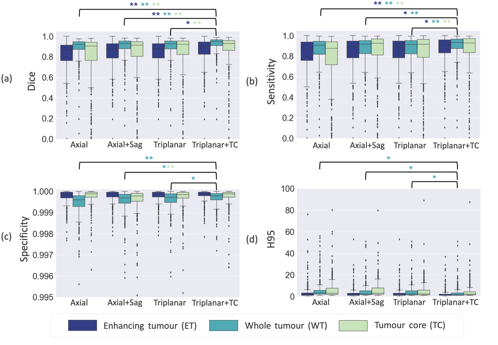
Figure 3: Boxplots of results from the ablation study, showing (a) Dice, (b) sensitivity, (c) specificity and (d) H95 for axial, axial+sagittal, triplanar and triplanar+TC cases. Significant differences in performance metrics are indicated by asterisks (* - p $<$ 0.01, ** - p $<$ 0.001) in the corresponding colours for tumour sub-regions. Note that only the significant differences in performance metrics between triplanar+TC and other cases are shown (for all combinations of individual pairs, refer to table 2).

Evaluation on the unlabelled validation data: The models trained from the 5-fold cross-validation of the training data were applied to the validation data and the final predictions were obtained using majority voting (from 5 models). The results obtained from the online evaluation platform are shown in table 3. A few sample validation data outputs of our method are shown along with input modalities in fig. 4. The results followed a trend similar to the training data obtaining the best results for WT segmentation with mean Dice and H95 values of 0.89 and 4.4 respectively.

Table 3: Results for BraTS’20 Validation data.

	Dice			Sensitivity			Specificity			H95 (mm)
	ET	WT	TC	ET	WT	TC	ET	WT	TC	ET	WT	TC
Mean	0.77	0.89	0.77	0.76	0.87	0.73	0.99	0.99	0.99	29.4	4.4	15.3
Std.	0.27	0.09	0.27	0.29	0.13	0.29	.0005	.0009	.0003	96.2	5.4	57.3
Median	0.87	0.93	0.90	0.88	0.91	0.86	0.99	0.99	0.99	2.0	3.0	3.0
25 quantile	0.77	0.89	0.73	0.74	0.85	0.61	0.99	0.99	0.99	1.0	2.0	1.7
75 quantile	0.91	0.95	0.94	0.94	0.95	0.93	0.99	0.99	0.99	3.6	4.6	8.5
ET - enhancing tumour, WT - whole tumour, TC - tumour core.

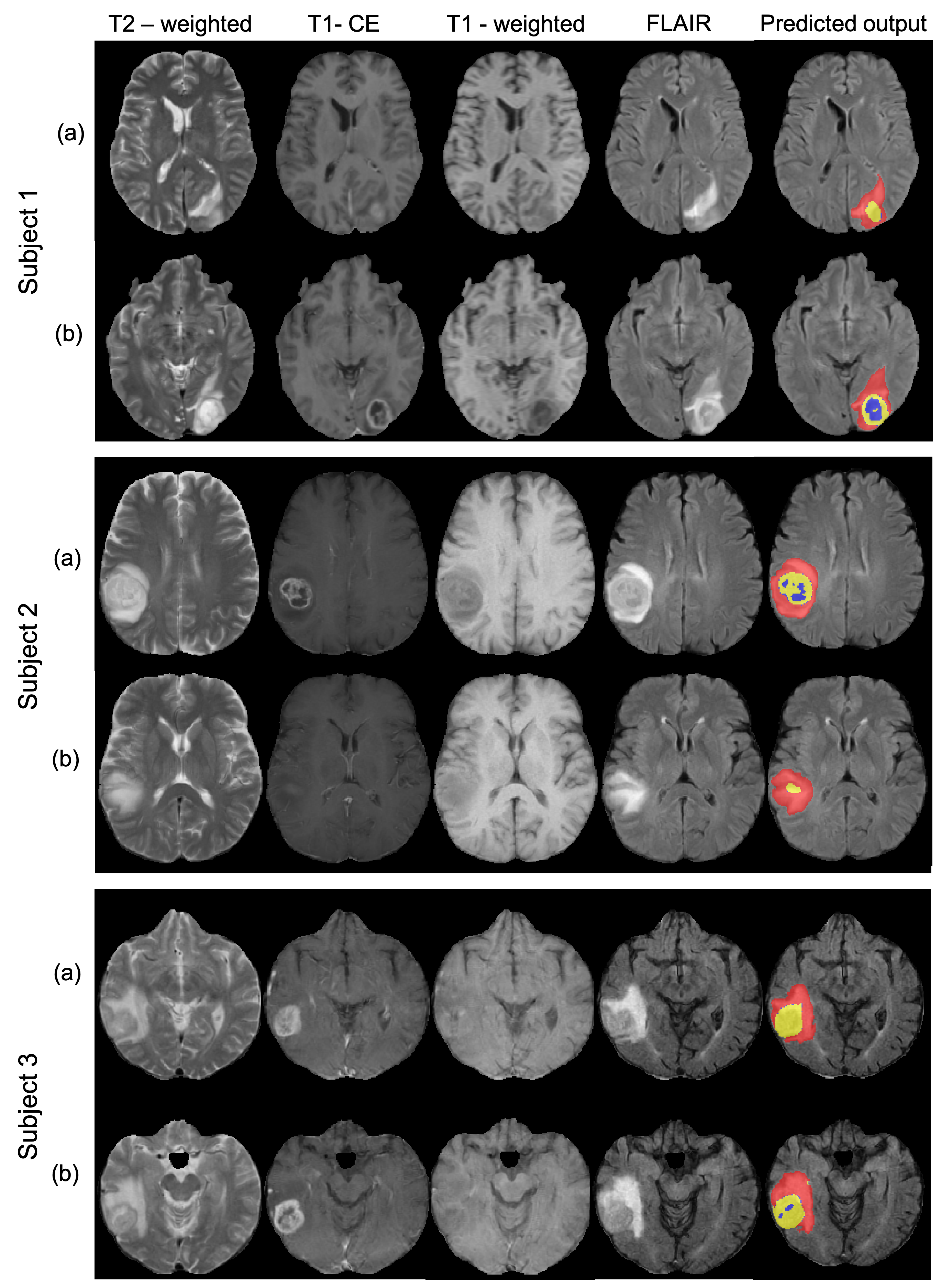
Figure 4: Results on BraTS’20 validation data from three sample subjects. Predicted outputs on two axial slices (a) and (b) from from three sample subjects (NCR/NET - blue, ET - yellow and ED - red), along with the provided input modalities: T2-weighted, T1-CE, T1 and FLAIR. Subject1: Dice (ET/WT/TC) - 0.86/0.97/0.96, sensitivity (ET/WT/TC) - 0.81/0.96/0.98, specificity (all) - 0.99, H95 (ET/WT/TC) - 1.4/1/1 mm; Subject2: Dice (ET/WT/TC) - 0.93/0.97/0.96, sensitivity (ET/WT/TC) - 0.93/0.99/0.97, specificity (all) - 0.99, H95 (all) - 1 mm; Subject3: Dice (ET/WT/TC) - 0.95/0.93/0.95, sensitivity (ET/WT/TC) - 0.97/0.99/0.98, specificity (all) - 0.99, H95 (ET/WT/TC) - 1/2/1 mm.

Results on the unseen test data: Finally, the results obtained from the online evaluation platform on the BraTS’20 test data are shown in table 4. Similar to the validation stage, majority voting on the results of 5 models (from 5-fold cross-validation) was used to predict the tumour region labels. As seen from the table, the Dice values for the WT region was higher than for the ET and TC regions as in the case of the validation stage. However, the Dice and sensitivity values for the ET and TC regions were considerably higher than those on the validation data, and were almost on par with those obtained with the fold-validation on the training dataset.

Table 4: Results for BraTS’20 Test data.

	Dice			Sensitivity			Specificity			H95 (mm)
	ET	WT	TC	ET	WT	TC	ET	WT	TC	ET	WT	TC
Mean	0.81	0.89	0.84	0.84	0.88	0.83	0.99	0.99	0.99	15.3	6.3	15.2
Std.	0.20	0.11	0.24	0.21	0.13	0.25	.0004	.0007	.0007	69.5	28.9	63.9
Median	0.85	0.92	0.92	0.92	0.92	0.94	0.99	0.99	0.99	1.4	2.8	2.2
25 quantile	0.78	0.87	0.87	0.83	0.86	0.82	0.99	0.99	0.99	1.0	1.7	1.4
75 quantile	0.93	0.95	0.96	0.96	0.96	0.97	0.99	0.99	0.99	2.2	4.8	3.8
ET - enhancing tumour, WT - whole tumour, TC - tumour core.

4 Discussion and conclusions

In this work, we proposed an end-to-end automated tumour segmentation method using a triplanar ensemble architecture of 2D U-Nets. Our method segmented ET, WT and TC sub-regions of the tumour with dice values of 0.83, 0.93 and 0.87 on the training dataset. On an independent unlabelled validation dataset, our method achieved Dice values of 0.77, 0.89 and 0.77 for ET, WT and TC sub-regions respectively. On the BraTS’20 unseen test dataset, our method achieved the Dice values of 0.81, 0.89 and 0.84 for the ET, WT and TC regions respectively.

Studying the effect of individual components on segmentation performance aided in better understanding the proposed method. For all the tissue classes, a single axial network performs the worst, probably due to the lack of contextual information from the contiguous slices. The triplanar architecture provides better performance than the individual 2D networks with higher Dice and sensitivity values. Moreover, we achieved significant improvement in the performance metrics with the addition of a specific TC network, especially for the TC class. The WT segmentation improves with the addition of each component and the significantly lower H95 values indicate a more precise tumour segmentation.

From the results on the training and validation data, performance for the WT is higher than for the other two classes, indicating that the method segments the cumulative tumour region (including the edematous/invaded region) with higher accuracy than the differentiation between core and edema. However, a few misclassified tumour core regions were due to cases where the ET class is very small (as indicated by white arrows in fig. 2). This results in ET either being incorrectly predicted (by the network) or falsely relabeled (in the post-processing step) as a part of the NCR/NET class. This substantially affects the Dice score for the ET class for the subject. In general, we observed that applying generalisable/consistent prior information or post-processing operations for TC and ET classes was not possible due to the wide range of tumour characteristics and variation in ground truth, which presented a major challenge for the segmentation task. Interestingly, for the TC region, our method performed better on the training and the unseen test datasets when compared to the validation dataset, as observed from the higher values of the metrics in tables 1 and 4 as compared to those in table 3. The higher values on the training dataset could be due to the fact that the cross-validation results are generally more prone to over-fitting, and hence are less reliable when compared to the results on the unseen validation data. However, our method also provided consistently good performance on the unseen test dataset (table 4). Since this was an unseen dataset, we cannot exclude the possibility that the tumour characteristics and image intensity profiles of the test dataset could be more similar to those of the training dataset.

On the BraTS’20 unseen test dataset, our method achieved higher Dice values compared to the validation Dice values, obtaining an evaluation score that was equal 5^th highest and 10^th place in the overall ranking in the challenge. As an indirect comparison with existing methods using different validation datasets, our method achieved a Dice value of 0.89 (on the BraTS’20 validation dataset) for the WT class, comparable to the top-ranking methods of BraTS’17-19 ($\sim$0.90) [7], [21], [14], [18], [19] and a Dice value of 0.77 for the ET class, on par with top-ranking methods of BraTS’17 ($\sim$0.78) [7], [21]. It is worth noting that even though the previous BraTS challenges used data from different subjects, this indirect comparison could be quite useful in determining the potential of our method, since the comparison involves the same task and type of data.

Summarising, our proposed triplanar ensemble method achieves accurate segmentation of whole tumours and their sub-regions on brain MR images from multimodal data of the BraTS’20 challenge. After the challenge, we will make our method publicly available as a Docker container that could be used as an independent tumour segmentation tool. Future directions include further improvement of tumour sub-region segmentation by leveraging the salient features (e.g. using attention networks).

References

- [1] B. H. Menze, A. Jakab, S. Bauer, J. Kalpathy-Cramer, K. Farahani, J. Kirby, et al. ”The Multimodal Brain Tumor Image Segmentation Benchmark (BRATS)”, IEEE Transactions on Medical Imaging 34(10), 1993-2024 (2015) DOI: 10.1109/TMI.2014.2377694
- [2] S. Bakas, M. Reyes, A. Jakab, S. Bauer, M. Rempfler, A. Crimi, et al., ”Identifying the Best Machine Learning Algorithms for Brain Tumor Segmentation, Progression Assessment, and Overall Survival Prediction in the BRATS Challenge”, arXiv preprint arXiv:1811.02629 (2018)
- [3] S. Bakas, H. Akbari, A. Sotiras, M. Bilello, M. Rozycki, J.S. Kirby, et al., ”Advancing The Cancer Genome Atlas glioma MRI collections with expert segmentation labels and radiomic features”, Nature Scientific Data, 4:170117 (2017) DOI: 10.1038/sdata.2017.117
- [4] S. Bakas, H. Akbari, A. Sotiras, M. Bilello, M. Rozycki, J. Kirby, et al., ”Segmentation Labels and Radiomic Features for the Pre-operative Scans of the TCGA-GBM collection”, The Cancer Imaging Archive, 2017. DOI: 10.7937/K9/TCIA.2017.KLXWJJ1Q
- [5] S. Bakas, H. Akbari, A. Sotiras, M. Bilello, M. Rozycki, J. Kirby, et al., ”Segmentation Labels and Radiomic Features for the Pre-operative Scans of the TCGA-LGG collection”, The Cancer Imaging Archive, 2017. DOI: 10.7937/K9/TCIA.2017.GJQ7R0EF
- [6] S. Pereira, A. Pinto, V. Alves, and C.A. Silva. ”Brain tumor segmentation using convolutional neural networks in MRI images.” IEEE transactions on medical imaging 35, no. 5 (2016): 1240-1251.
- [7] K. Kamnitsas, C. Ledig, V.F. Newcombe, J.P. Simpson, A.D. Kane, D.K. Menon, et al. ”Efficient multi-scale 3D CNN with fully connected CRF for accurate brain lesion segmentation.” Medical image analysis 36 (2017): 61-78.
- [8] M. Havaei, A. Davy, D. Warde-Farley, A. Biard, A. Courville, Y. Bengio, et al. ”Brain tumor segmentation with deep neural networks.” Medical image analysis 35 (2017): 18-31.
- [9] H. Shen, R. Wang, J. Zhang, and S.J. McKenna. ”Boundary-aware fully convolutional network for brain tumor segmentation.” In International Conference on Medical Image Computing and Computer-Assisted Intervention (MICCAI), pp. 433-441. Springer, Cham, 2017.
- [10] K. Kamnitsas, W. Bai, E. Ferrante, S. McDonagh, M. Sinclair, N. Pawlowski, et al. ”Ensembles of multiple models and architectures for robust brain tumour segmentation.” In International MICCAI Brainlesion Workshop, pp. 450-462. Springer, Cham, 2017.
- [11] R. McKinley, R. Meier, and R. Wiest. ”Ensembles of densely-connected CNNs with label-uncertainty for brain tumor segmentation.” In MICCAI Brainlesion Workshop, pp. 456-465. Springer, Cham, 2018.
- [12] R. McKinley, M. Rebsamen, R. Meier, and R. Wiest. ”Triplanar Ensemble of 3D-to-2D CNNs with Label-Uncertainty for Brain Tumor Segmentation.” In MICCAI Brainlesion Workshop, pp. 379-387. Springer, Cham, 2019.
- [13] T. Yang, Y. Ou, and T. Huang. ”Automatic segmentation of brain tumor from MR images using SegNet: selection of training data sets.” In Proc. 6th MICCAI BraTS Challenge, pp. 309-312. 2017.
- [14] A. Myronenko. ”3D MRI brain tumor segmentation using autoencoder regularization.” In MICCAI Brainlesion Workshop, pp. 311-320. Springer, Cham, 2018.
- [15] O. Ronneberger, P. Fischer, and T. Brox. ”U-net: Convolutional networks for biomedical image segmentation.” In MICCAI, pp. 234-241. Springer, Cham, 2015.
- [16] G. Kim. ”Brain tumor segmentation using deep fully convolutional neural networks.” In MICCAI Brainlesion Workshop, pp. 344-357. Springer, Cham, 2017.
- [17] F. Isensee, P. Kickingereder, W. Wick, M. Bendszus and K.H. Maier-Hein. ”Brain tumor segmentation and radiomics survival prediction: Contribution to the brats 2017 challenge.” In MICCAI Brainlesion Workshop, pp. 287-297. Springer, Cham, 2017.
- [18] F. Isensee, P. Kickingereder, W. Wick, M. Bendszus, and K.H. Maier-Hein. ”No new-net.” In International MICCAI Brainlesion Workshop, pp. 234-244. Springer, Cham, 2018.
- [19] Z. Jiang, C. Ding, M. Liu, and D. Tao. ”Two-Stage Cascaded U-Net: 1st Place Solution to BraTS Challenge 2019 Segmentation Task.” In MICCAI Brainlesion Workshop, pp. 231-241. Springer, Cham, 2019.
- [20] V. Sundaresan, G. Zamboni, P. M. Rothwell, M. Jenkinson, and L. Griffanti. ”Triplanar ensemble U-Net model for white matter hyperintensities segmentation on MR images.” BioRxiv (2020). https://doi.org/10.1101/2020.07.24.219485.
- [21] G. Wang, W. Li, S. Ourselin and T. Vercauteren. ”Automatic brain tumor segmentation using cascaded anisotropic convolutional neural networks.” In MICCAI brainlesion workshop, pp. 178-190. Springer, Cham, 2017.