Observable scattered light features from inclined and non-inclined planets embedded in protoplanetary discs

Abstract

Over the last few years instruments such as VLT/SPHERE and Subaru/HiCIAO have been able to take detailed scattered light images of protoplanetary discs. Many of the features observed in these discs are generally suspected to be caused by an embedded planet, and understanding the cause of these features requires detailed theoretical models. In this work we investigate disc-planet interactions using the PLUTO code to run 2D and 3D hydrodynamic simulations of protoplanetary discs with embedded 30 M_⊕ and 300 M_⊕ planets on both an inclined ($i=2.86^{\circ}$) and non-inclined orbit, using an $\alpha$-viscosity of $4\times 10^{-3}$. We produce synthetic scattered-light images of these discs at H-band wavelengths using the radiative transfer code RADMC3D. We find that while the surface density evolution in 2D and 3D simulations of inclined and non-inclined planets remain fairly similar, their observational appearance is remarkably different. Most of the features seen in the synthetic H-band images are connected to density variations of the disc at around 3.3 scale heights above and below the midplane, which emphasizes the need for 3D simulations. Planets on sustained orbital inclinations disrupt the disc’s upper-atmosphere and produce radically different observable features and intensity profiles, including shadowing effects and intensity variation in the order of 10-20 times the surrounding background. The vertical optical depth to the disc midplane for H-band wavelengths is $\tau\approx 20$ in the disc gap created by the high-mass planet. We conclude that direct imaging of planets embedded in the disc remains difficult to observe, even for massive planets in the gap.

1 Introduction

Planets are formed in the accretion discs of interstellar gas and dust around young stellar objects (YSOs). As these discs are believed to be regions of early planet formation and incubation, they are commonly referred to as protoplanetary discs. The planet formation process itself is not directly observable due to the distances to these YSOs, the relatively small sizes of protoplanets, and that the newly forming planets are obscured within their host disc. Therefore, one of the most observationally accessible ways of understanding planet formation is by studying protoplanetary discs via multi-wavelength observations. By comparing the observations with theoretical models, we can better understand these discs themselves as planet-forming regions, as well as how the presence of a newly forming planet affects their dynamics and evolution.

Accretion discs have been studied for decades, with theoretical models developed for their structure and evolution (e.g., Shakura & Sunyaev, 1973; Pringle, 1981). Later, properties of passive accretion discs specifically around YSOs, such as scale height, temperature profiles, and vertical structure were modeled from theory and observations (Kenyon & Hartmann, 1987; Chiang & Goldreich, 1997; D’Alessio et al., 1998). These model-disc profiles, combined with more readily available computational clusters, allowed theorists to explore how planets interact gravitationally with their host disc, and how the dynamics of the disc evolve with time via two-dimensional and three-dimensional hydrodynamic (HD) simulations (e.g., Bate et al., 2003; Varnière et al., 2004; Crida & Morbidelli, 2007; Edgar & Quillen, 2008). These simulations revealed that planets can greatly affect their host disc, creating features such as spiral arms and density gaps due to displaced material in the orbital vicinity of the planet. See reviews by Armitage (2011), Williams & Cieza (2011), and Kley (2017) for a more complete description of protoplanetary discs.

Recent technological advances have shown evidence that there may indeed be material gaps in protoplanetary discs seen in near-infrared (near-IR) wavelength observations in the form of dark rings, e.g. in TW Hya seen with Subaru (Akiyama et al., 2015) and in HD 169142 seen with VLT/SPHERE/ZIMPOL (Bertrang et al., 2018). Other features like large-scale spiral-arm structures have also been seen in near-IR observations of protoplanetary discs, such as SAO 206462 (Garufi et al., 2013) and MWC 758 (Benisty et al., 2015). Spirals have been accompanied by shadowing effects in HD 100453 (Benisty et al., 2017), and possible vortices and spirals caused by a planet in the HD135344B transition disc (van der Marel et al., 2016), as well as shadows cast on HD 135344B from multiwavelength VLT/SPHERE polarimetric differential imaging (Stolker et al., 2016).

As the observations merely capture a snap-shot in time, and the planets themselves are not visible, a common strategy for protoplanetary disc simulations is to vary conditions such that the observable features can be recreated, then offer these conditions as a possible description of the protoplanetary system. The dark and bright rings commonly seen in observations have successfully been recreated in simulations from planets displacing material within their orbit and creating material gaps in the disc (e.g., Juhász et al., 2015; Dong & Fung, 2017b). Keppler et al. (2018) and Müller et al. (2018) recently observed the first stellar companion within the gap of a still-intact transitional disc, giving the results from these models derived via disc-planet simulations new weight. However, recent HD simulations have been able to produce multiple gaps in a disc with only a single embedded planet (Zhu et al., 2014; Dong et al., 2017; Bae et al., 2017) suggesting it is possible that not every observed gap is due to an individual planet.

Synthetic images from hydrodynamic simulations have also been able to create observed spiral features in discs, usually as a result of the presence of a massive planet or other stellar companion (Dong et al., 2015a, b; Dong et al., 2016). These kinds of simulations have been able to successfully reproduce the spiral arms observed in systems such as SAO 206462 with a 10-15 M_J companion (Bae et al., 2016), and HD 100453 using a 0.2 M_⊙ companion, which is actually observed in the system (Wagner et al., 2018). Although theories that do not require the presence of a planet have been suggested to explain spiral arms (e.g., disc shadowing (Montesinos et al., 2016)), the success of disc-companion simulations in recreating observable features of specific systems demonstrate that planets can visibly affect their host disc.

These kinds of two- and three-dimensional simulations, combined with follow-up synthetic images, are essential in understanding protoplanetary systems because of the relatively small number of clearly observable discs. In most cases limitations in resolution or obscuration make directly observing the object responsible for producing the spiral-arm or gap features observed in some of these discs impossible or impractical. Simulating disc-planet interactions present the possibility of identifying the causes of these observed features, and models derived from simulations also have the potential to estimate planet properties based on its effects on the disc.

The simulations used to model the observed systems discussed above used a simplifying assumption that the orbit of the planet is aligned with the midplane of the disc, ignoring the possibility of planetary interactions causing orbital inclinations. Although it is unknown whether this kind of misalignment can be produced or sustained while the gas of the disc is still present, the idea of non-ideal planet-disc interactions (i.e. planets with non-zero orbital inclinations and eccentricities) has been of interest for years (Marzari & Nelson, 2009; Bitsch et al., 2013; Sotiriadis et al., 2017; Chametla et al., 2017), with more recent studies exploring changes in observable features of discs containing inclined planets, such as Arzamasskiy et al. (2018) and Zhu (2019).

Here we continue this exploration by comparing two- and three-dimensional simulations of protoplanetary discs with an embedded planet. In the case of the three-dimensional simulations, we simulate this disc-planet evolution for planets with orbits aligned and mis-aligned with the disc midplane. In all cases we produce synthetic images of how these simulated discs would be observed in near-infrared wavelengths using a Monte-Carlo radiative transfer method. We present our methods and initial conditions for our hydrodynamic simulations in §2. Specific parameters used for the discs and the results of the HD simulations are given in §3 and the synthetic images as results from our radiative transfer simulations in §4. In §5 we discuss these results, explore how orbital inclination damping would affect observable features in §5.4, and derive conclusions from these results in §6.

2 Numerical Methods

2.1 Hydrodynamics

We model the dynamics and evolution of protoplanetary discs as a fully 3-dimensional, viscous, locally isothermal (no energy equation), hydrodynamic system governed by the equations of conservation of mass and momentum

$$\frac{\partial\rho}{\partial t}+\nabla\cdot\rho\mathbf{v} = 0$$ (1)

$$\frac{\partial\mathbf{m}}{\partial t}+\nabla\cdot\left(\mathbf{mv}+\ P\mathbf{I}\right) = \ -\rho\nabla\Phi+\nabla\cdot\mathbf{\Pi}$$ (2)

where $\rho$ is the mass density, $\mathbf{m}=\rho\mathbf{v}$ is the momentum density, $\mathbf{v}$ is the velocity, $P$ is the thermal pressure, $\mathbf{I}$ is the unit tensor. $\Phi$ is the softened gravitational potential due to the central star and the planet, which is

$$\Phi=-\frac{GM_{*}}{r}-\frac{GM_{p}}{\sqrt{(\left|\mathbf{r}-\mathbf{r_{p}}\right|)^{2}+\epsilon^{2}}},$$ (3)

where $r=\left|\mathbf{r}\right|$ is the distance to the star and $\left|\mathbf{r}-\mathbf{r_{p}}\right|$ is the distance to the planet located at $\mathbf{r_{p}}$. We use a spherical coordinate system, with radial, polar, and azimuthal variables as $\mathbf{r}$ = ($r,\theta,\phi$), unless otherwise specified since it is especially suited to describe the gravitational potentials of a planet with mass $M_{p}$ rotating around a central star of mass $M_{*}$. The softening parameter is some fraction of the Hill radius, $\epsilon=kr_{\mbox{\scriptsize H}}$, where

$$r_{\mbox{\scriptsize H}}\equiv r_{p}\left(\frac{M_{p}}{3M_{*}}\right)^{1/3}$$ (4)

and we use a value of $k=0.3$ throughout the series of simulations. Viscous stresses are handled via the viscous stress tensor, $\mathbf{\Pi}$, with components given by

$$(\Pi)_{ij}=\mu_{1}\left(\frac{\partial v_{i}}{\partial x_{j}}+\ \frac{\partial v_{j}}{\partial x_{i}}\right)+\ \left(\mu_{2}-\frac{2}{3}\mu_{1}\right)\nabla\cdot\mathbf{v}\delta_{ij}$$ (5)

where $\mu_{1}$ and $\mu_{2}$ are the coefficients of shear and bulk viscosity. We use the typical $\alpha$-viscosity prescription of Shakura & Sunyaev (1973) defined as

$$\nu=\alpha c_{s}H$$ (6)

where $\nu$ is the kinematic turbulent viscosity, which is related to the coefficient of shear viscosity in Eqn. (5) as

$$\mu_{1}=\nu\rho$$ (7)

and assume a coefficient of bulk viscosity as $\mu_{2}=0$, typical for low-density density gases not experiencing hypersonic compression or expansion.

In order to solve the conservation equations (1) and (2), we use the numerical code PLUTO v4.2 (Mignone et al., 2007), a modular, finite volume, shock-capturing code. We choose a piecewise total variation diminishing linear reconstruction integrator, which is 2nd order accurate in space, and specified the use of a monotonized central difference limiter (MC_LIM). We applied a 2nd order Runge-Kutta time integrator, a Courant-Friedrichs-Lewy (CFL) number of 0.3, and in all cases we ran PLUTO with the FARGO module to save computational time.

All simulations use an isothermal equation of state standard in the PLUTO code, which defines the relation between gas density and pressure as

$$P=c_{s}^{2}\rho$$ (8)

where $c_{s}$ is the sound speed of the gas. Assuming an ideal gas, the relation between $c_{s}$ and gas temperature, $T_{g}$, is

$$c_{s}^{2}=\frac{k_{b}T_{g}}{\mu m_{p}}$$ (9)

where $k_{b}$ is the Boltzmann constant, $\mu$ is the mean molecular weight, and $m_{p}$ is the mass of a proton. For a protoplanetary disc, a typical used value for the mean molecular weight is $\mu=2.3$, to represent a gas composition consists primarily of molecular hydrogen, plus a smaller amount of heavier elements.

For a thin disc in hydrostatic and thermal equilibrium that is heated only by radiation from a central host star, the gas temperature profile can be approximated as being vertically isothermal for the disc interior, depending only on the distance from the host star (Kenyon & Hartmann, 1987). This approximation is consistently used in similar hydrodynamic and magnetohydrodynamic simulations of protoplanetary discs (Uribe et al., 2011; Nelson et al., 2013), and in this case the gas temperature is proportional to a power-law as $T_{g}\propto(r\sin\theta)^{q}$, which from Eqn. (9) implies $c_{s}^{2}\propto(r\sin\theta)^{q}$. We modified the PLUTO code so that this sound-speed profile could be included in the equation of state.

2.2 Initial and Boundary Conditions

To derive the initial conditions it is useful to use a cylindrical coordinate system, with radial, azimuthal, and vertical variables as $\mathbf{R}$ = ($R,\phi,z$), where spherical and cylindrical radial coordinate variables are related as $R=r\sin\theta$. These conditions are derived from Eqn. (2) for a non-viscous circumstellar disc ($\mathbf{\Pi}=0$) without a planet,

$$\frac{\partial\mathbf{v}}{\partial t}+\left(\mathbf{v}\cdot\nabla\right)\mathbf{v}\ =-\frac{1}{\rho}\nabla P-\nabla\Phi_{*},$$ (10)

where $\Phi_{*}=GM_{*}/(R^{2}+z^{2})^{1/2}$ is the gravitational potential due only to the central star. In both models the disc is in hydrostatic equilibrium in the radial and vertical directions, has a mid-plane density of

$$\rho_{\mbox{\scriptsize c}}(R)=\rho_{0}\left(\frac{R}{R_{0}}\right)^{p}$$ (11)

and a radially dependent gas sound-speed of

$$c_{s}^{2}(R)=c_{0}^{2}\left(\frac{R}{R_{0}}\right)^{q}$$ (12)

where $R_{0}$ is the initial orbital radius of the planet, $\rho_{0}$ is the mid-plane density at $R_{0}$, $c_{0}^{2}$ is the square of the sound speed at $R_{0}$, and $p$ and $q$ are power law indices. Separating Eqn. (10) into its vertical and radial components

$$0 = \frac{1}{\rho}\frac{\partial P}{\partial z}+\ \frac{GM_{*}}{(R^{2}+z^{2})^{3/2}}z$$ (13)

$$R\Omega^{2} = \frac{1}{\rho}\frac{\partial P}{\partial R}+\ \frac{GM_{*}}{(R^{2}+z^{2})^{3/2}}R.$$ (14)

Initial profiles for $\rho(R,z)$ and $\Omega(R,z)$ come from solving Eqs. (13) and (14) directly, with solutions from Nelson et al. (2013):

$$\rho(R,z) = \rho_{0}\left(\frac{R}{R_{0}}\right)^{p}\ \exp\left(\frac{GM}{c_{s}^{2}}\left[\frac{1}{\sqrt{R^{2}+z^{2}}}-\ \frac{1}{R}\right]\right)$$ (15)

$$\Omega(R,z) = \Omega_{k}\left[(p+q)\left(\frac{H}{R}\right)^{2}+(1+q)-\ \frac{qR}{\sqrt{R^{2}+z^{2}}}\right]^{1/2}$$ (16)

where $\Omega_{k}=\sqrt{GM/R^{3}}$ is the Keplerian angular velocity at radius $R$, and $H\equiv c_{s}/\Omega_{k}$ is the thermal scale height of the disc. The evolution of our planet’s orbit is determined by parameterized equations in Cartesian coordinates

$$x_{p}(t) = -R_{0}\cos(\Omega_{k}t)$$ (17)

$$y_{p}(t) = -R_{0}\sin(\Omega_{k}t)\cos(i)$$ (18)

$$z_{p}(t) = -R_{0}\sin(\Omega_{k}t)\sin(i)$$ (19)

where $t$ is time, and $i$ is the angle of inclination of the planet with respect to the midplane of the disc. Setting $R_{0}=1$, this corresponds to the initial location of the planet being at $\mathbf{r_{0}}=(r_{0},\theta_{0},\phi_{0})=(1,\pi/2,\pi)$ in our simulation units. The location of the star was held fixed at the origin.

We use a computational domain of $r\in[0.3,3.5]$, $\theta\in[1.3258,1.8158]$, and $\phi\in[0,2\pi]$, with a uniform grid of $(N_{r},N_{\theta},N_{\phi})=(400,98,786)$ cells, which allows us to resolve one vertical scale height with 10 cells at the orbital radius of the planet. The parameters used for the basic setup of all our hydrodynamic simulations are summarized in Table 1.

We allow the planet to grow to full mass over the course of 10 orbits so the disc in hydrostatic equilibrium is not suddenly disrupted by the appearance of a gravitational potential. Azimuthal boundary conditions are periodic, and we use a zero-gradient outflow condition at the polar boundaries which forces ghost-cell velocity values to zero if they are directed back into the disc. To prevent mass loss, ghost cells at the radial boundaries are fixed at initial conditions.

Figure 1: Time evolution of normalized disc surface density for simulations involving planets with orbits aligned with the disc midplane (Top) and misaligned with the disc (Bottom). Dotted ($\cdot\cdot$) lines show the state of the disc at $t=200$ orbits, Dash-dotted ($-\cdot-$) lines are at $t=300$ orbits, dashed ($--$) lines are at $t=400$ orbits, and the solid lines ($-$) are at $t=1000$ orbits. The depth of the dips in surface density have essentially reached a steady state.

Figure 2: Surface density maps of the 2D (Left), 3D non-inclined (Centre), and 3D inclined (Right) planetary-orbit simulations with 30 M_⊕ (Top) and 300 M_⊕ (Bottom) planets.

3 HD Simulation Setup & Results

3.1 Simulation Setup

We simulated a flared protoplanetary disc with a sound speed profile of $q=-1/2$ in Eqn. (12) to mimic a passive irradiated disc, which corresponds to a thermal scale-height profile of

$$H=H_{0}\left(\frac{R}{R_{0}}\right)^{5/4},$$ (20)

where $H_{0}$ is the thermal scale-height at $R_{0}$. With this profile, we used a central density index of $p=-7/4$ in Eqn. (11) in order to keep an initial surface density profile of

$$\Sigma_{i}=\Sigma_{0}\left(\frac{R}{R_{0}}\right)^{-1/2},$$ (21)

where $\Sigma_{0}$ is the surface density of the unperturbed disc at $R_{0}$. We set $H_{0}=0.05R_{0}$, which bounds the simulation to 5$H$ above and below the midplane at the location of the planet. In all simulations we use a constant $\alpha$-viscosity parameter of $\alpha=4.0\times 10^{-3}$.

We studied the evolution of a 3D disc with an embedded planet whose orbit was aligned with the disc’s midplane ($i=0^{\circ}$). We considered planets with a mass of 30 M_⊕ (model 3D30A) and one of 300 M_⊕ (3D300A). Other previous works have shown the presence of a planet will carve gaps in azimuthally averaged surface density plots of protoplanetary discs (e.g., Bate et al., 2003; Crida et al., 2006). Exploratory test runs of our HD simulations revealed similar gaps, and we used the depth of these gaps to determine the duration of the simulations. We ran the 30 M_⊕ and 300 M_⊕ planet simulations until the azimuthally averaged surface densities in the vicinity of the planet (i.e. the depth of the gap) had essentially reached a steady-state. This corresponded to the 30 M_⊕ planet simulations being run for $\sim$200 orbits and the 300 M_⊕ planet simulations for $\sim$400 orbits, but we extended the 30 M_⊕ planet simulations out to 400 orbits and the 300 M_⊕ planet simulation out to 1000 orbits. 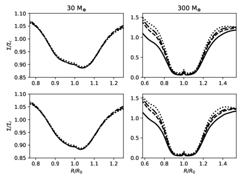This is demonstrated in Figure 1, which shows the time evolution of the azimuthally averaged surface density near the location of the planet at $t=200,300,$ and $400$ orbits of the 30 M_⊕ and 300 M_⊕ planets, as well as at $t=1000$ orbits of the 300 M_⊕ planet. This plot shows that the gap profile has converged.

For comparison, we ran simulations in which the disc evolved with a planet orbiting at a sustained slight incline with respect to the disc. We chose an inclination of $i=2.86^{\circ}$, which corresponds to approximately one thermal scale-height above the midplane at the apex of the orbit. We performed these inclined orbit simulations again using a 30 M_⊕ planet (3D30I), as well as a 300 M_⊕ planet (3D300I). We also created 2-dimensional equivalent simulations of discs with embedded 30 M_⊕ (2D30) and 300 M_⊕ (2D300) planets for 400 and 1000 orbits, respectively, using the same resolution and conditions described in §2.2, with an initial surface density profile of $\Sigma_{i}=\Sigma_{0}\left(R/R_{0}\right)^{-1/2}$. In these 2D simulations we used values of $p=-1/2$ and $z=0$ for our initial conditions in Eqns. (15) and (16), as well as an equation of state of $P=\Sigma c_{s}^{2}$. However, by their nature 2D simulations can not include information about the vertical dynamics or the dynamics of the material above over below the planet. Analysis and simulations of discs by Müller et al. (2012) and Kley et al. (2012) showed that in order for the results from 2D simulations to be in agreement to their 3D counterparts, the softening parameter for the gravitational potential (Eqn. 3) must be increased to $\epsilon=0.7H$ when self-gravity is not taken into consideration. We therefore include this correction to our 2D simulations.

Model parameters for each of our simulations are summarized in Table 2.

Table 1: Physical parameters used for the general setup of hydrodynamic simulations.

Parameter	Symbol	Value
Stellar mass	$M_{*}$	M☉
Orbital radius	$R_{0}$	1.
Thermal scale-height at $R_{0}$	$H_{0}$	0.05$R_{0}$
Alpha viscosity	$\alpha$	$4\times 10^{-3}$
Number of grid cells	$N_{r}\times N_{\theta}\times N_{\phi}$	$400\times 98\times 786$
Radial resolution	$\Delta r$	$4H_{0}/25$
Polar resolution at $r_{0}$	$r_{0}\Delta\theta$	$H_{0}/10$

3.2 300 M_⊕ Planet Results

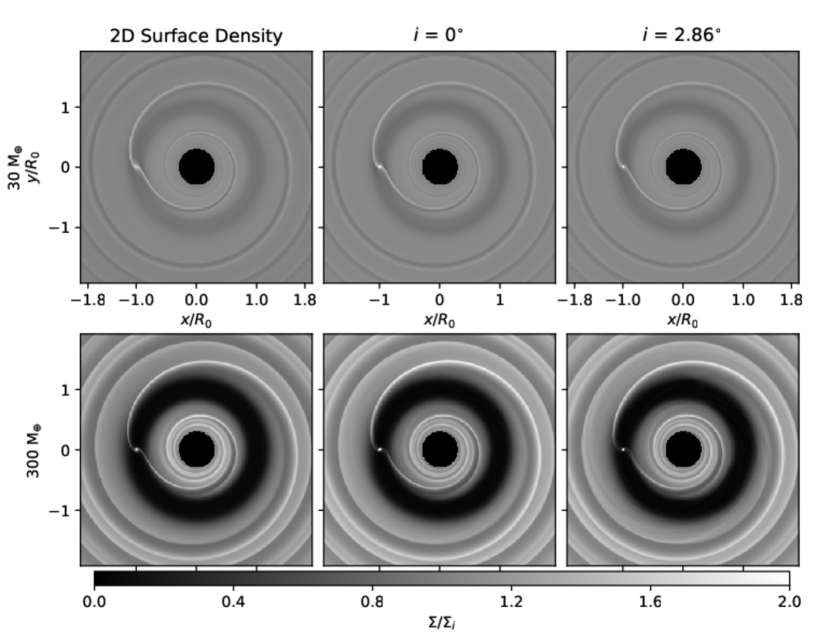
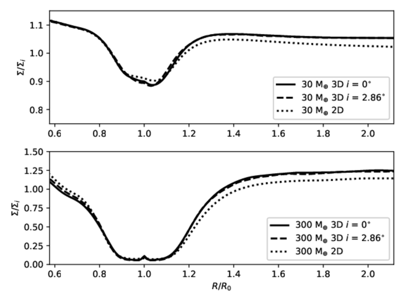
Final global surface density features for each simulation are presented as maps in Figure 2, as well as azimuthally averaged profiles in Figure 3. In the case of the 300 M_⊕ planet simulations, the features produced from the disc-planet interaction were independent of the dimensionality of the simulation or whether the orbit of the planet was aligned with the disc. In all three cases the planet creates an annular low-density region in the orbital vicinity of the planet, as well as primary spiral-density arms which emanate inwards and outwards from the planet. A secondary arm can also be seen in each simulation inwards of the planet’s orbit around $(x/R_{0},y/R_{0})=(0.75,0)$, along with the possibility of a tertiary near $(-0.5,0)$. These various arms are expected as even tertiary arms have been seen in similar hydrodynamic simulations of discs with embedded high-mass planets (e.g., Dong & Fung, 2017a).

The similarities in simulations involving the 300 M_⊕ planet are even more obvious when presented in Figure 3 (Bottom). As seen in similar HD simulations (e.g., Bate et al., 2003; de Val-Borro et al., 2006; Uribe et al., 2011), the high-mass planet created a substantial gap in its vicinity. The depth, width, and general shape of this gap is remarkably unaffected by the variations of each simulation. Kanagawa et al. (2015a); Kanagawa et al. (2015b) contributed to developing a relationship between the depth of such gaps as

$$\frac{\Sigma_{\mbox{\scriptsize min}}}{\Sigma_{i}}=\frac{1}{1+0.04K},$$ (22)

where $\Sigma_{\mbox{\scriptsize min}}$ is the surface density at the bottom of the gap,

$$K=\left(\frac{M_{p}}{M_{*}}\right)^{2}\left(\frac{H}{R}\right)^{-5}\alpha^{-1},$$ (23)

and, again, $\Sigma_{i}$ is the surface density of the unperturbed disc.

With this as a basis, Zhu (2019) derived a relation for the expected gap depth caused by an inclined planet, using a new value for $K$ as

$$K=\left(\frac{M_{p}}{M_{*}}\right)^{2}\left(\frac{H}{R}\right)^{-5}\alpha^{-1}\frac{4}{\pi^{2}(n+1)}\ \left[\mathcal{K}\left(\frac{n}{n+1}\right)\right]^{2},$$ (24)

where $n=(R_{0}{\sin}(i)/H)^{2}$, $\mathcal{K}(m)$ is the complete elliptic integral of the first kind, with $m$=$k^{2}$, and $k$ is the elliptic modulus.

Values derived from Eqn. (22) predict that slight orbital inclinations of high-mass planets do not significantly affect gap depth, a feature that is also demonstrated in the simulations explored in this work. Although Figure 3 suggests that in all three cases depths of the gaps in surface density produced by a 300 M_⊕ planet are essentially identical, the numerical values of $\Sigma_{\mbox{\scriptsize min}}/\Sigma_{i}$ show variations between each other and the predicted values (Table 2). In each of our simulations, the depth of the gap is not quite as great as the predicted values, especially in the case of the 2D simulation. When compared to results from other simulations (e.g., Varnière et al., 2004; Duffell & MacFadyen, 2013), and Fung et al. (2014), Eqn. (22) does fit rather well, even though there is a fairly large spread in this fit (See Figure 1 of (Kanagawa et al., 2015b)).

As the results from our simulations involving a high-mass planet are within this spread, we can consider them to be in reasonable agreement with the predicted values, as well as other work. However, It should be noted that many of the simulations from Varnière et al. (2004), Duffell & MacFadyen (2013), and Fung et al. (2014) were run for several thousand to 20,000 orbits to generate the values of their gap depths, and the limitations on the duration of these simulations due to their three-dimensional nature could be the cause of this discrepancy between simulation and prediction. While it is not likely that these small differences in gap depth would drastically effect the observable features, it would be worth a single extended simulation dedicated to test this assumption.

Table 2: Summary of hydrodynamic disc models and parameters used in simulations. Columns: 1) Model name, 2) Dimensions, 3) Planet mass, 4) Number of orbits at $R=R_{0}$, 5) Power-law index for initial $\rho$ (Eqn. 15), 6) Orbital inclination of planet (in degrees), 7) Gravitational potential softening parameter (Eqn. 3), 8) Maximum gap depth from simulation, 9) Maximum predicted gap depth (Eqn. 22). All simulations used a power-law index of $q=-1/2$ for $c_{s}^{2}$ (Eqn. 12).

Model	Dimensions	Planet Mass	Orbits	$p$	$i$	$\epsilon$	Gap Depth	Predicted Depth
							$\Sigma_{\mbox{\scriptsize min}}/\Sigma_{i}$	$\Sigma_{\mbox{\scriptsize min}}/\Sigma_{i}$
(1)	(2)	(3)	(4)	(5)	(6)	(7)	(8)	(9)
2D30	2D	30 M⊕	400	-1/2	-	0.7$H$	0.90	0.80
3D30A	3D	′′	300	-7/4	$0^{\circ}$	0.2$H_{0}$	0.89	′′
3D30A	3D	′′	400	-7/4	$0^{\circ}$	′′	0.89	′′
3D30I	3D	′′	300	-7/4	2.86∘	′′	0.88	0.85
3D30I	3D	′′	400	-7/4	2.86∘	′′	0.88	′′
2D300	2D	300 M⊕	1000	-1/2	-	0.7$H$	0.070	0.037
3D300A	3D	′′	300	-7/4	$0^{\circ}$	0.4$H_{0}$	0.083	′′
3D300A	3D	′′	700	-7/4	$0^{\circ}$	′′	0.061	′′
3D300A	3D	′′	1000	-7/4	$0^{\circ}$	′′	0.059	′′
3D300I	3D	′′	700	-7/4	2.86∘	′′	0.057	0.053
3D300I	3D	′′	1000	-7/4	2.86∘	′′	0.055	′′

Figure 3: Azimuthally averaged surface density profile, $\Sigma$, normalized by initial surface density, $\Sigma_{i}$, for the 30 M_⊕ (Top) and 300 M_⊕ (Bottom) simulations for planet orbits aligned with the disc (solid, $-$), misaligned with the disc (dashed, $--$), and 2D discs (dotted, $\cdot\cdot$). Results from the 30 M_⊕ planet simulations are after 400 orbits, and after 1000 orbits for the 300 M_⊕ planet simulations.

3.3 30 M_⊕ Planet Results

Figures 2 and 3 also show results of our hydrodynamic simulations involving the 30 M_⊕ planet after 400 orbits. As in the 300 M_⊕ planet situation, the surface density maps show no obvious differences regardless of the dimensionality of the simulation or the alignment of the planet. In each case spiral density waves are emitted radially inwards and outwards from the planet, causing a primary spiral arm coiling towards the inner boundary. A secondary arm can also be seen near $(x/R_{0},y/R_{0})=(0,-0.75)$ in Figure 2 in all three cases, but these maps lack the tertiary arm seen in the simulations involving a high-mass planet. While the average surface density values are slightly lower in the 2D simulations radially outwards from the planet, the general shape of the profile is essentially the game. One notable difference is the slightly deeper depths in averaged surface densities in the 3D cases compared to the 2D case (see Figure 3 and Table 2), however this difference is quite small.

Values presented in Table 2 do show a discrepancy between the gap depths from the simulations compared to those predicted from Eqn. (22), even though this ratio of $\Sigma_{\mbox{\scriptsize min}}/\Sigma_{i}$ remained constant from $t=200-400$ orbits (Figure 1). Predicted values of gap depths are almost 10% greater than what the 2D and 3D simulations show. This is not a slight discrepancy which could simply be attributed to scatter, as in the case of the high-mass planet simulation.

With our fixed boundary conditions, material moving radially outwards is not allowed to leave the system. To test if this hindered the low-mass planet’s ability to displace material, causing the discrepancy between simulation and predicted gap depth, we tested our 3D30A model using outflow conditions at the radial boundaries. With this set up, our gap depth was $\Sigma_{\mbox{\scriptsize min}}/\Sigma_{i}=0.89$ at $t=200$ orbits, but dropped to $\Sigma_{\mbox{\scriptsize min}}/\Sigma_{i}=0.88$ from $t=200-400$, slightly deeper than with the fixed boundary conditions. We then extended the run out ever further to find that the gap depth increased very slowly where it finally reached a value of $\Sigma_{\mbox{\scriptsize min}}/\Sigma_{i}=0.87$ at $t=800$.

While the outflow conditions do show the gap depth to continue to increase over time, we see diminishing returns similar to those seen in the 300 M_⊕ simulations; where several hundred orbits are required to increase the gap depth by a very small amount. However, in the case of the high-mass planet simulation, the gap was essentially made by $\sim$400 orbits, and begin to slowly approach its predicted value of the course of the next several hundred orbits. In the case of this low-mass planet, the gap is slowly increasing, but it is still no where near the predicted value of $\Sigma_{\mbox{\scriptsize min}}/\Sigma_{i}=0.80$ after 800 orbits.

Since the depth of this gap is slowing growing over time with the outflow bounds, it is possible it would match its predicted value after several thousand, or tens of thousands, of orbits, as mentioned in §3.2. However, is also possible that the gap depth is increasing because using outflow boundary conditions for a viscous disc result in an overall mass loss, with the total mass of the disc decreasing by 23% over the first 400 orbits, and by 32% after 800 orbits. This drastic loss of material in the inner and outer disc could affect observational features produced from these models, making much longer runs not viable. Likewise, fixing the radial boundaries at initial conditions does slightly increase the mass of the disc over time (4% after 400 orbits), also limiting the effective duration of these simulations.

Although gap depths for the 2D30, 3D30I, 3D30A, and 3D30A-Outflow do not match predicted values, they are consistent with each other, displacing $\sim$10-13% of initial material in the vicinity of the planet. We continue to use the results from these simulations throughout this paper, but consider the implications of if gap from the low-mass planet had reached its predicted depth in §4.1.

4 Synthetic Images

Figure 4: Synthetic scattered light H-band images of the 2D (Left), 3D non-inclined (Centre), and 3D inclined (Right) planetary-orbit simulations with 30 M_⊕ (Top) and 300 M_⊕ (Bottom) planets. The actual location of the planet is indicated by a star symbol.

We created synthetic images of how our model discs would be observed in the H-band (1.65 $\mu$m) using the Monte Carlo radiative transfer code RADMC3D v0.41 (Dullemond et al., 2012) (see Appendix A for details).

For the two-dimensional simulations we extrapolated a 3-dimensional density profile from the resultant surface density values, $\Sigma(R,\phi)$, by assuming surface density and density are related as

$$\rho(r,\theta,\phi)=\frac{\Sigma(R,\phi)}{\sqrt{2\pi}H}\ \exp\left(\frac{GM}{c_{s}^{2}}\left[\frac{1}{r}-\ \frac{1}{R}\right]\right),$$ (25)

using the same 3D domain and grid, along with the $H$ and $c_{s}^{2}$ profiles, described in §2.2. We also significantly decreased the density in the $10\times 10$ set of grid cells surrounding the location of the planet before making the 3-dimensional extrapolation to minimize the shadowing effect from having a physically unrealistic column of high-density material.

4.1 30 M_⊕ Planet Images

Figure 5: Azimuthally averaged H-band ($\log_{10}(I_{\lambda})$ $\lambda=1.65$ $\mu$m) scattered light from the 30 M_⊕ planet simulations. Top: Intensity dip at the location of the planet (5.2 au) for 3D30A model (Dashed, $--$), and the 2D30 model (Dash-Dotted, $-\cdot-$), compared to the intensity of an unperturbed disc (solid, $-$). Also included are results from simulation in which the surface density gap reached the predicted depth from Eqn.(22) (doted, $\cdot\cdot$). Bottom: Intensity plot for the 3D30I model, extended out to disc radius of 9 au to show global disturbances of the disc. Dashed ($--$) line shows the averaged intensity of the disc as viewed from the top, while the Dotted ($\cdot\cdot$) line is viewed from the bottom, compared to the intensity of an unperturbed disc (Solid, $-$). Intensity features of the inclined planet show no obvious indication of a planet located at 5.2 au.

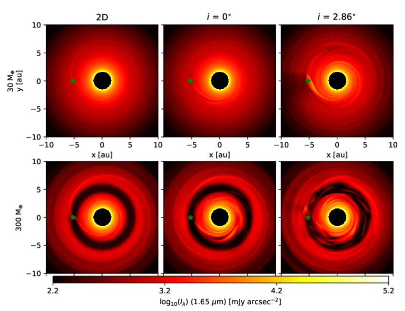
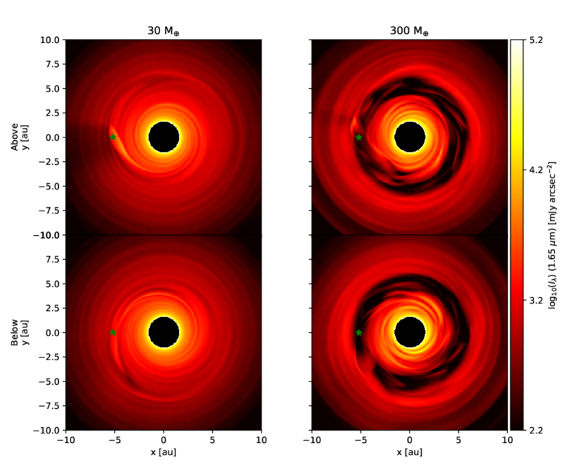
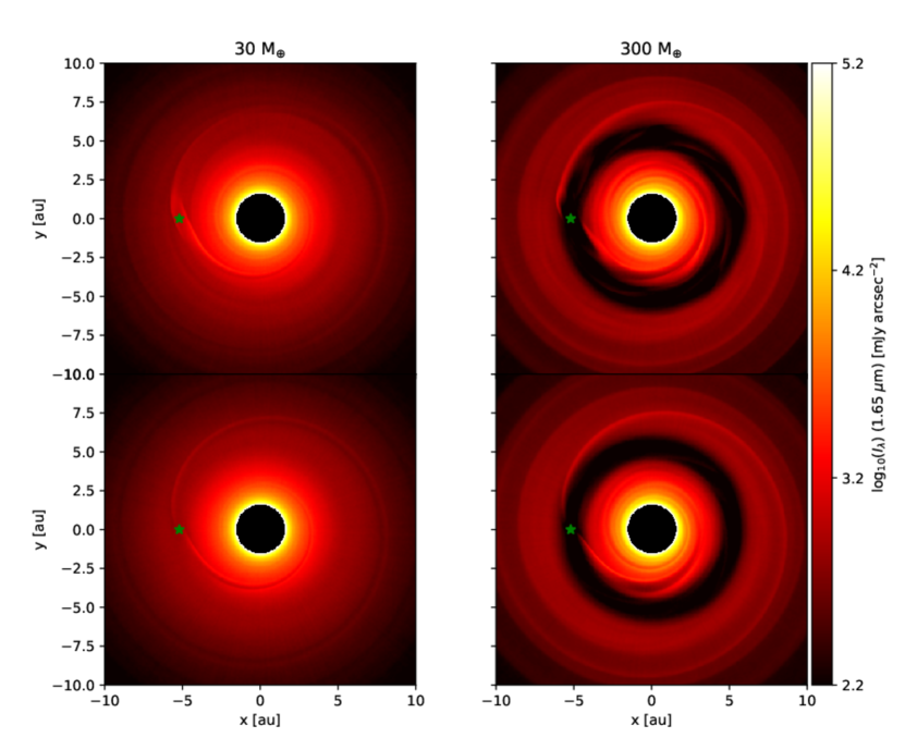
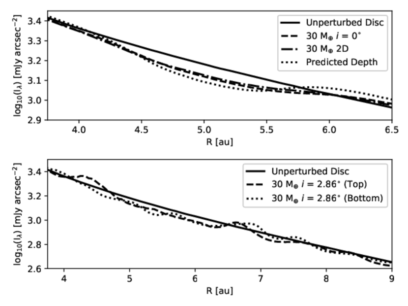
In Figure 4 (Top) we show the face-on H-band synthetic images produced from the results of the 30 M_⊕ planet HD simulations, and plot the azimuthally averaged intensity profiles in Figure 5. Images from the 2D30 and 3D30A models bear close resemblance to each other, and to their respective surface density maps (Figure 2), including signs of their primary spiral density waves and secondary arms. Unlike the surface density maps, there is no feature in the scattered light images which immediately indicate the displacement of material from the planet (i.e., a dark annular region), however the effect of the surface density gap can be seen in Figure 5 (Top), which shows a small decrease in average intensity near the vicinity of the planet. This intensity is 87-88% of the profile of the unperturbed disc, which corresponds with the depth of the surface density gap. This intensity dip seen in both the 2D30 and 3D30A models suggests that H-band observation have the potential to infer the presence of these lower-mass planets, as such small deviations are found in VLT/SPHERE observations (e.g., Bertrang et al., 2018). Aside from this, the synthetic image of the 3D30A model shows a distinct gap between the primary and secondary arms, making the existence of the secondary arm much more apparent.

While the synthetic image of the 2D30 model does not reveal any more information than its corresponding surface density map, and the 3D30A image very closely resembles its own surface density map, the image produced from the inclined 30 M_⊕ planet model (3D30I) is significantly different. In this image the primary arms are severely disrupted and the inclined orbit produces that appears around the location of the planet, which casts a shadow with an azimuthal arc of 30^∘.

In the case of 30 M_⊕ planet with an inclined orbit, there is also no obvious indication of the dark annular region observed in the images from the non-inclined models. This lack of intensity drop at the radial location of the planet is seen more clearly in Figure 5 (Bottom), which extends the average intensity profile out to 9 au. From this plot it is apparent that the intensity drops caused by planets with non-inclined orbits can be distinguished from the background, but disruptions from the inclined planet create several hills and valleys in this profile which are no where near the location of any planet.

As mentioned in §3.3, the maximum depth of the surface density gap caused by a 30 M_⊕ planet is not quite as deep as predictions would indicate. In running preliminary simulations used to test the models in this paper, we found that when running 2D simulations involving low-mass planets without the increased gravitational softening parameter discussed in §3.1, the depth of the gap did agree with predicted values ( $\Sigma_{\mbox{\scriptsize min}}/\Sigma_{i}=0.80$ ) after only 200 orbits. By extrapolating the results from this simulation into a 3D distribution, then applying the radiative transfer process described in Appendix A, we can compare average intensity features of the predicted results to those from our models. Results from this analysis are included in Figure 5 (Top), and reveal an intensity that is approximately 82% of the unperturbed profile. This also corresponds fairly well to the depth of the surface density gap, and does demonstrate that small changes in surface density could have an effect on scattered light observations for ideal situations such as a single-planet system perfectly aligned with the disc. Figure 5 (Bottom) shows non-ideal situations such as mis-aligned planetary orbits, do not produce a similar relation between surface density and scattered light features.

4.2 300 M_⊕ Planet Images

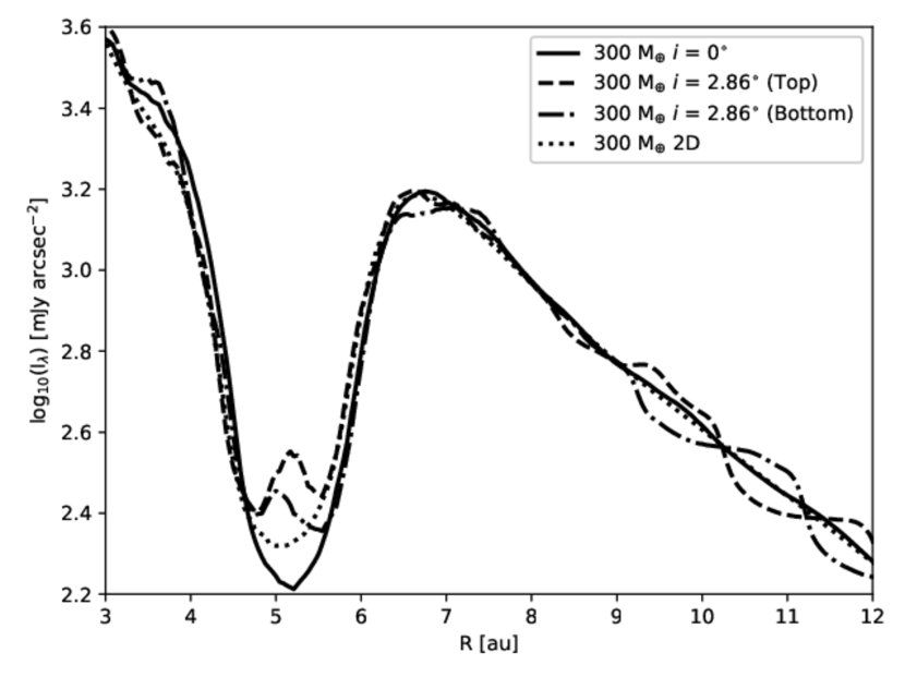
Figure 4 also shows the synthetic scattered light images from the 300 M_⊕ planet models, with their azimuthally averaged intensity plots in Figure 6. As with the 30 M_⊕ planet simulations, images produced from the 2D300 and 3D300A models have similar characteristics with each other, and their surface density maps (Figure 2). The dark annular region at the planet’s orbit is clearly apparent in both cases, along with the presence of primary, secondary, and tertiary arms. However, while the synthetic image from the 2D300 model does not reveal any additional features compared to its surface density map, the features seen in the 3D300A model image are slightly different; with signs of material remaining in the gap, as well as the emergence of a dark, spiral-arm-like feature near $(x,y)=(0,-4)$ au, between the primary and secondary arms that makes the existence of the secondary arm much more apparent.

Despite the similarities seen in their surface density features (Figures 2 & 3), when their intensities are azimuthally averaged over the entire disc, as shown in Figure 6, it seems that the slight differences between the surface density gap depth from models 2D300 and 3D300A (Table 2) produce obvious differences in intensity profiles. When compared to the inclined model 3D300I, the dark annular region of the synthetic image in Figure 4 shows a significant amount of turbulent material within this region that is less apparent than in the other two models. The spiral arms are also highly disrupted, which makes it more difficult to distinguish them from each other, or properly identify them. There is also a compact shadow-producing feature near $(x,y)=(-5.6,1.6)$ au. The location of this feature is especially noteworthy as its size and morphology could possibly be seen as evidence of a directly imaged, newly forming planet in an actual observation, however the planet in this simulation is actually located at $(x,y)=(-5.2,0)$ at the disc’s midplane. The depth of the dip in the averaged intensity profile at the radial location of the planet for model 3D300I is also not as deep as the other high-mass planet simulations, and the intensity shows hills and valleys at larger radii nowhere near the planet, similar to the inclined lower-mass planet simulation.

Figure 6: Azimuthally averaged H-band ($\log_{10}(I_{\lambda})$ $\lambda=1.65$ $\micron$) scattered light intensity for the 300 M_⊕ planet. Solid ($-$) line is intensity values from model 3D300A, while the Dashed ($--$) and Dash-Dotted ($-\cdot-$) lines are intensity values from model 3D300I as view from the top and bottom of the disc, respectively. Model 2D300 is represented by the Dotted ($\cdot\cdot$) line. In all cases there is a clear and obvious dip at the location of the planet (5.2 au), however the maximum depth of the dip varies. The inclined planet also produces waves at the outer radius, where intensity peaks from one point of view seemingly correspond to intensity dips from the other.

5 Discussion

5.1 2D vs. 3D Simulations

We used RADMC3D to calculate the height of the surface where, from the aspect of an observer, the optical depth is $\tau_{s}=2/3$ for a wavelength $\lambda=1.65$ $\mu$m ( i.e., the observed surface). Applying this to our unperturbed density profile, we found that this surface is 3.3 thermal scale-heights above the midplane at $R=R_{0}$.

As the two-dimensional simulations are simply surface density evolutions of disc-planet interactions, it is not surprising that producing synthetic scattered light images using density structures that have been vertically extrapolated from 2D structures are essentially replications of these surface density features. This should be expected regardless of the height of the surface. The gas dynamics of the 3D simulations, however, are not necessarily vertically invariant.

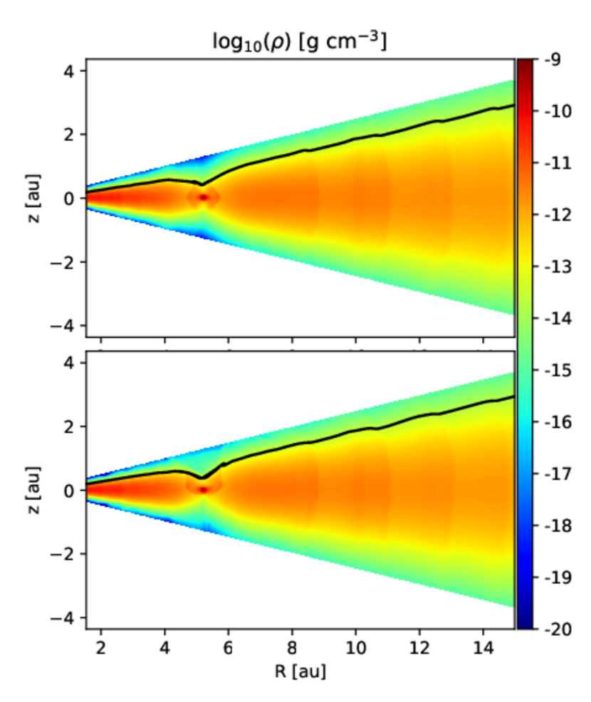
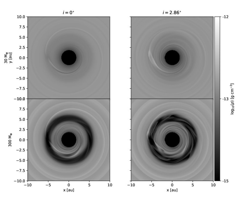
Figure 7 shows examples of vertical density maps of the two 3D simulation results involving the 300 M_⊕ planet, as well as the profile of the observed surface superimposed onto the map. It should be noted that throughout this section we present lengths in au, with intensity and density values in cgs units, using the conversions described in Appendix A. With this observed surface being so high above the disc midplane, it is also not surprising the surface density maps of the 3D simulations in Figure 2, essentially midplane features, are not exactly the same as their corresponding synthetic scattered light images. From this it would seem that H-band images, synthetic and actual, reflect the disc’s upper-atmospheric conditions. To help confirm this, Figure 9 shows density slices at $\theta=80.7^{\circ}$ (the height of the scatter surface of an unperturbed disc at $R=R_{0}$) from the results of our four 3D models. The features seen in these upper-atmosphere density maps much more closely resemble those in the scattered-light images of Figure 4 than the surface density maps in Figure 2. Although not visible in the 2D simulation, these features include wisps of material can be clearly seen in the annular ring created by the 300 M_⊕ planet in the 3D simulations. This demonstrates the possibility that despite a planet almost completely clearing out disc material at the midplane, gas remnants could still be present in the gap at the disc’s upper-layers; a feature models from 2D simulations would miss.

Figure 7: Density map of vertical slice at the location of the 300 M_⊕ planet for the $i=0^{\circ}$ simulation (Top) and the $i=2.86^{\circ}$ simulation (Bottom). The solid black line indicates the $\tau_{s}=2/3$ surface of the disc for light of wavelength $\lambda=1.65$ $\mu$m.

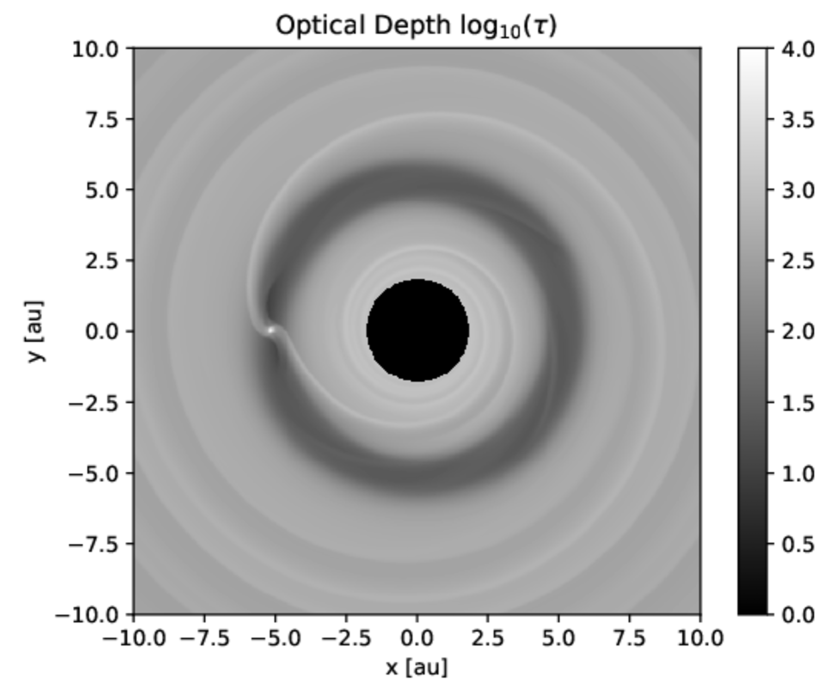
To demonstrate the difficulty of near-IR observations to see into the midplane, we approximate the optical depth from an observer to the midplane via,

$$\tau_{\lambda}=\int_{\theta_{0}}^{\pi/2}\rho_{d}\kappa_{\lambda}r~{}d\theta,$$ (26)

where $\theta_{0}$ is the upper polar boundary of the disc, $\rho_{d}$ is the dust density, and $\kappa_{\lambda}=1320$ cm² g^-1 is total dust opacity at a wavelength $\lambda=1.65\micron$ (from Figure 16). Figure 8 shows this applied to the 3D300A simulation. Certain areas near the planet in the $\pm$y-direction have an optical depth as small as $\tau=10$, but at the orbital radius of the planet the optical depth is $\tau\approx 20$, even when 94% of the initial material has been removed. Directly observing midplane features in these discs at near-IR wavelengths, or directly observing a planet within the disc, would not be feasible.

Figure 8: $\log_{10}$ map of optical depth for light of wavelength $\lambda=1.65\micron$ at the midplane of simulation 3D300A. In general, the optical depth at $R=R_{0}$ (the center of the gap) is $\tau\approx 20$.

That these scattered light images are looking at the upper layers of protoplanetary discs raises the question of whether synthetic images produced from 2D simulations can reliably model the observable near-IR features of these discs. Works such as Ruge et al. (2014) and Zhu et al. (2015) argue that in order to realistically model these discs, and their observable properties, fully 3D models are required for reasons such as that 2D simulations can “overestimate the detectability of planet-induced gaps” and spiral arms are much more prominent in synthetic images produced from 3-dimensional simulations. On the other hand, Fung & Chiang (2016) compare surface density profiles of 2D and 3D hydrodynamic simulations to show they are similar, and Dong & Fung (2017b) compare synthetic H-band images of an example Saturn-mass planet produced from 2D and 3D hydrodynamic simulations to justify the use of 2D simulations for modeling observable disc features. Our results seem to be in agreement with the idea that under ideal conditions, 3D density extrapolations from 2D simulations are sufficient to create models of scattered light images, as the uncertainty of planet mass estimates from disc observations is typically quite large (e.g., Fedele et al., 2017; Müller et al., 2018). For interactions in which the planet’s effects on the disc are not vertically invariant, however, models from fully three-dimensional simulations are required.

Figure 9: Density maps of the 3D simulations cut along the polar angle of $\theta=80.7^{\circ}$, corresponding to the angle of the $\tau_{s}=2/3$ surface of an unperturbed disc at $R=R_{0}$. Results shown are for planets with non-inclined orbits (Left), and inclined (Right) for simulations involving a 30 M_⊕ planet (Top) and a 300 M_⊕ (Bottom). These upper-atmosphere density maps resemble the synthetic images seen in Figure 4 much more than those of the surface density maps in Figure 2.

5.2 Inclined Orbits

Figures 2 and 3 show that in the cases of the 3D hydrodynamic simulations, slight planet inclinations seem to have no effect on the features seen in the surface density maps, or the average surface density profile, for both the high- and low-mass planets. However, Figures 4, 5, 6, and 9 all show that an inclined planet does have a significant impact on the gas dynamics of the discs at the height of the scatter surface, as well as a significant impact on the scattered light features and intensity of near-IR observations. The ability for an inclined planet to alter the gas dynamics of the upper-atmosphere is expected considering the added vertical component of the planet’s motion. As long as small ($\sim$$\micron$) dust grains are able to remain coupled to the turbulent gas at the surface, this significant effect on the near-IR observable features is also expected. We explore how reducing the amount of dust in the upper atmosphere would affect our observations in Appendix B.

Figures 5 and 6 also show that there are large radial variations in average intensity throughout the disc for the inclined-planet simulations. As the depth of some of these intensity variations in the 3D300I model are greater than the intensity gap produced in 3D30A, in actual observations these kinds of variations could be falsely perceived as signatures of multiple planets, or even as secondary gaps in the disc due to shock waves caused by a single massive planet (e.g., Bae et al., 2017). Models attempting to interpret such observations using the assumption that the planet is co-orbital with the disc would obtain incorrect results. Likewise, these large radial variations in intensity are not necessarily evidence for an inclined planet. As seen in Figure 4 (Bottom-Right), the variations in average intensity are likely caused by the disruption of the spiral density arms in the disc’s upper-atmosphere, which could be the result of any regular disruption.

The density maps of Figure 9 and the the synthetic scattered light images of Figure 4 show that not only do scattered light images show the upper-atmospheric features of the disc, but that some of these features cause shadows which could affect the temperature and overall dynamics of the disc. One of these features is particularly noteworthy; a small bright area which resembles an overdense region, and causes a shadow, in the inclined 300 M_⊕ planet simulation (Figure 4, Bottom-Right). A similar feature, a bright point-like object, has been observed in the $L^{\prime}$-band in the transitional disc HD169142 which was considered to be a potential 28-32 M${}_{\mbox{\scriptsize Jup}}$ companion object, however the absence of this bright point source in $H$-band or $K_{s}$-band makes it more likely that is is a disc feature and not a planet (Biller et al., 2014; Reggiani et al., 2014). Our simulations have produced a bright point-like feature which could be interpreted as a newly forming planet or brown dwarf companion object, however we know for a fact that there is no planet at the location of this feature.

The cause of this bright area in 3D300I is a high density region of gas near the upper-boundary of the simulation that appears to be connected to the outer spiral density wave. This could potentially be a result of the disc-planet exchange which produces spiral density waves is occurring at varying levels of the disc, creating a much more complicated dynamic. This amorphous high-density region is located between 4-5$H$ above (but not below) the disc midplane, but begins to disappear at around 3.5$H$ (Note this high-density area is not as prominent in Figure 9, which is a density slice at 3.3$H$). While the exact cause of this feature unknown, the feature appears quite early in the simulation ($\sim$30 orbits), which gave us the opportunity to run several short exploratory trials.

1. Increased the cell numbers in the radial and azimuthal dimensions to provide uniform grid resolution at $R=R_{0}$.

2. Radial boundary conditions were set to outflow.

3. Outflow conditions at the polar boundaries were slightly altered such that the density values in the ghost cells were linearly extrapolated from domain values, rather than simple zero-gradient.

In all cases this high-density region persisted. We also decreased the vertical size of the simulation to $\pm$4$H$ at $R=R_{0}$, as well as $\pm$3$H$ at $R=R_{0}$. The density layers at the upper-boundaries of these smaller simulations matched very closely to those of the 4$H$ and 3$H$ density slices from the full simulation. The high-density region appears at the upper boundary of the 4$H$ simulation, but not at the upper boundary of the 3$H$ simulation, indicating that it is not simply due to an interaction between the gas and the boundary.

Analysis of radial, polar, and azimuthal velocities show that the gas dynamics at these layers of a disc with an inclined planet are far more complex than with an aligned planet. It is apparent that the high density region arises from this complex motion of the gas. By investigating with different boundaries this feature still remained. However we note due to the limitation of the model (e.g., simulating these complex upper-atmospheric dynamics at these scale heights using the vertically isothermal approximation) the physical nature of this feature should be taken with care.

Figure 10: Synthetic H-band (1.65 $\mu$m) scattered light maps involving the inclined 30 M_⊕ planet (Left) and the inclined 300 M_⊕ planet (Right) viewed from above (Top) and below (Bottom), with a star symbol indicating the location of the planet. The images are mapped such that from their respective points of view, the planet is rotating counter-clockwise as viewed from above, while it is rotating clockwise as viewed from below.

The shadow-causing feature seen in the synthetic image of the 3D30I model is also caused by a high-density region in the disc’s upper-atmosphere (Figure 9 Top-Right). This feature also follows the spiral density waves, and its origin is likely related to them and the complications that arise with these arms being produced at different heights in the disc. This dense region is extended, and in turn causes an extended shadow over a large part of the disc. The implications of this extend beyond the observable features discussed in this work, as the cooling of such a large region could have a profound effect on the evolution of the disc. To fully explore the consequences of shadowing on this scale, radiation hydrodynamic, or even radiation magnetohydrodynamic, simulations are required (Flock et al., 2013).

Another implication for observations is the asymmetry of the scattered light surfaces due to the inclined orbit of the planet. While azimuthally averaged intensity profiles do depend slightly on the inclination of the disc with respect to the observer (Dong & Fung, 2017b) if the orbit of a planet is aligned with the midplane, scattered light observations are essentially the same as viewed from the top of the disc as those viewed from the bottom. This is not the case when the the disc is asymmetric across the midplane, as demonstrated in Figure 10, which shows how the discs with inclined planets would be observed in scattered light as viewed from above and below. Despite that both points of view would be considered face-on observations, they show striking differences between each other; most notably the lack of a shadow cast by the disrupted spiral arm as viewed from the bottom in the lower-mass planet simulations. These different points of view also produce differences in average intensity profiles, as shown in Figures 5 & 6. Viewed from below, there is no obvious indication that there is a planet located at 5.2 au for the 3D30I model, and the intensity profile produces variations in intensity similar to those seen as viewed from the top. In the case of the 3D300I model, there is a clear indication of a planet at 5.2 au, which produces a dip in intensity slightly greater than its top-view counterpart. The view from the bottom also produces an interesting feature in that the peaks and valleys in intensity radially outwards from the planet are directly opposite to those as viewed from the top. As this is not seen in the lower-mass planet situation, further study is required to understand under what circumstances this occurs, or if it is simply an isolated incident. Comparing these results to follow up simulations in which the sign of Eqn. 19 is changed would also be a worth-while endeavor.

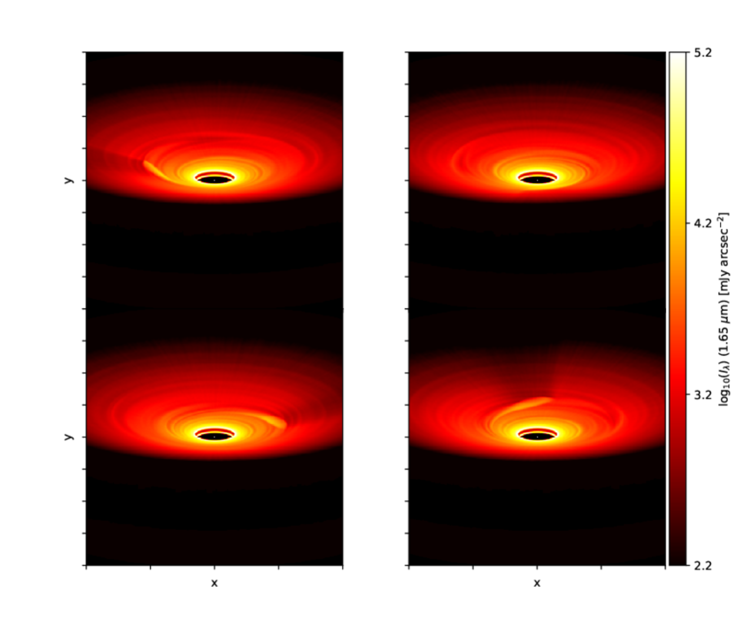
In spite of the shadow from features caused by inclined planets seen in Figure 4 can not be seen when the disc is viewed from below, Figure 11 shows that the massive massive shadow from the 3D30I model is visible even when the disc itself is inclined by $i_{d}=70^{\circ}$ from face-on. The shadow can also be seen at almost any rotational alignment of the disc, except when the disc is orientated such that the planet is between the star and the observer. It would seem that observations of discs with an embedded mis-aligned planet depend not only on disc inclination and orientation, but also whether the disc is being viewed from above or below.

Figure 11: Synthetic H-band (1.65 $\micron$) scattered light maps from the inclined 30 M_⊕ planet simulation (3D30I), observed with the disc inclined at $i_{d}=70^{\circ}$ (Top Left). Other images represent how the disc would be observed if it were rotated azimuthally anti-clockwise by $90^{\circ}$ (Top Right), $180^{\circ}$ (Bottom Left), and $270^{\circ}$ (Bottom Right).

5.3 Applications to Observations

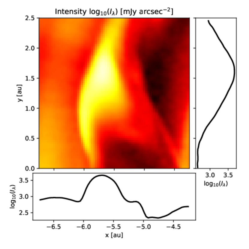
The bright features in our synthetic H-band images of discs with an embedded inclined planet are clearly visible in contrast to their surrounding intensity levels. This is demonstrated in Figure 12, which shows an intensity map of a $2.5\times 2.5$ au² area surrounding the small bright region seen near the planet in the 3D300I model. This map is accompanied by intensity slices at $x=-5.7$ au (Figure 12 Right), and $y=1.5$ au (Figure 12 Bottom). The intensity levels here can be up to twenty times higher than those in its immediate vicinity. This is also true in the feature seen in 3D30I, which is also larger and produces a shadow on the disc radially outwards from itself.

Figure 12: Intensity ($\lambda=1.65\micron$) map focused on bright region seen in the synthetic scattered light image of model 3D300I, along with a vertical intensity plot sliced at $x=-5.7$ au (Right) and a horizontal intensity plot sliced at $y=1.5$ au. The intensity of this bright region can be 20 times higher than the surrounding areas.

To explore the feasibility of actually observing these features, we placed them face-on at a distance of 100 parsecs and convolved them using a resolution of 0.03^′′ to approximate the capability of H-band observations from VLT/SPHERE. No features were resolvable at these scales, with the exception of the large shadow in the 3D30I model. This indicates that it is possible to detect extremely large-scale shadows without being able to identify the cause. It should be noted that van Boekel et al. (2017) has been able to resolve gaps at radii of less than 5.2 au using VLT/SPHERE for TW Hydrae at distance of 54 parsecs using polarized light. Synthetic scattered light images simulating polarized light at these scales will be considered for future work. While other instruments used to view protoplanetary discs, such as ALMA, have the resolution to observe a disc gap in TW Hydrae at 1 au (Andrews et al., 2016), these observations are at longer wavelengths which penetrate much deeper into the disc.

We also scaled the dust density from the 3D30I and 3D300I models and scaled them out to emulate our results for a planet orbiting at $R_{0}=30$ au, with a surface density of $\Sigma_{0}=30$ g cm^-2 and an aspect ratio of $H/R=0.07$ at $R=R_{0}$. With these new dust density profiles, we again used RADMC3D to create temperature and synthetic H-band images using the process described in Appendix A. 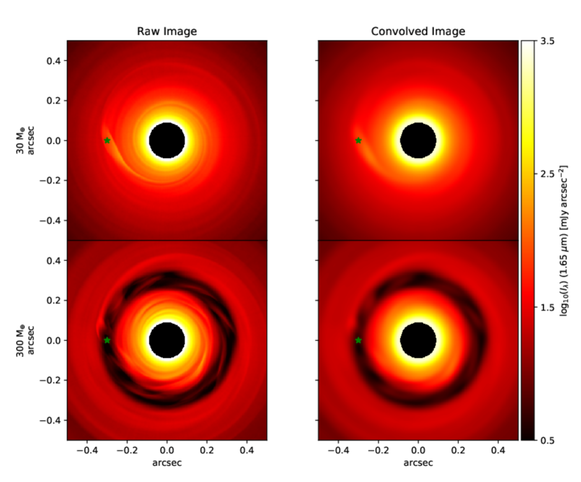We then convolved these images using the same distance and resolution described above (Figure 13). The feature caused by the 30 M_⊕ planet is still clearly visible, but no longer casts an obvious shadow. It is also distinguishable in the convolved image. 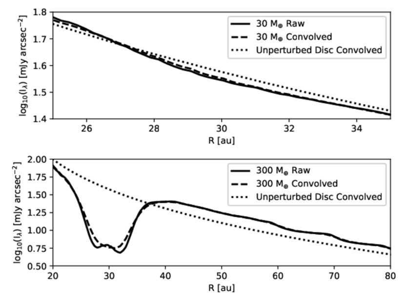There is also no obvious dark angular region at the orbital radius of the planet, although when the disc intensity is azimuthally averaged, as in Figure 14, the average intensity at the planet is 96% of an unperturbed disc.

The small bright feature from the 3D300I model is not as apparent as its 5.2 au counterpart, however, and is essentially non-existent in the convolved image. This is similar to the lower dust-to-gas models discussed in Appendix B. In this case the synthetic image also sees deeper into the disc, with a $\tau=2/3$ surface this is at only $0.7H$ at $R=R_{0}$, which effectively ignores aspects of the disc at the upper boundary. The average intensity is 15% of an unperturbed value, and the dark annular region at the location of the planet can be clearly seen in our convolved intensity map. Perturbations at the outer radius are also still apparent, similar to those seen in Figure 6. These dips can be as high as 10%, which are comparable to the depth caused by the 30 M_⊕ planet so could be mistaken for secondary planets.

Unfortunately there are severe limitations implementing radiative transfer techniques to this kind of scaling, namely in the difference of aspect ratios at 5.2 and 30 au. With our polar bounds, an aspect ratio of $H/R=0.07$ at $R_{0}=30$ au limits the vertical domain of the disc to $\pm 3.57H$ at the location of the planet. Evolving a full disc with more suitable initial density conditions could effect the dynamics in the upper-atmosphere, and including the dust distribution of the upper layers could raise the location of the observed surface. Future work involving observational features of protoplanetary discs caused by planets will focus on this region.

Figure 13: Synthetic H-band ($\lambda=1.54\micron$) images of the inclined 30 M_⊕ (Top) and 300 M_⊕ (Bottom) planet simulations scaled to $R_{0}=30$ au. Raw images are shown on the Left, while images convolved to resemble discs at 100 parsecs observed with a resolution of 0.03^′′ are shown on the Right.

Figure 14: Azimuthally averaged intensity values for images of discs involving the inclined 30 M_⊕ planet (Top) and inclined 300 M_⊕ planet (Bottom) at 30 au. The raw images (Solid, $-$) are compared to convolved images (Dashed, $--$), and to convolved images of unperturbed discs (Dotted, $\cdot\cdot$).

5.4 Damped Orbital Inclination

Although the difference in observable scattered light features between discs containing inclined and non-inclined planets is obviously apparent, other HD simulations have explored the evolution of inclined planets (e.g., Cresswell et al., 2007; Bitsch & Kley, 2011) and have found that for low-inclined planets (i.e. $i\la H/R$ ), orbital inclination of a planet decays exponentially, $di/dt\propto-i$. By varying a planet’s initial inclination and mass, and allowing the planet to move throughout the simulation, Bitsch & Kley (2011) determined that the damping time-scale was $\tau_{d}=53$ orbits for a planet at 5.2 au in an isothermal disc with a thermal scale-height of $(H/R)_{R_{0}}=0.05$, and $\tau_{d}=27$ orbits when radiative transfer effects where taken into account throughout the simulation. To explore how damping inclination would affect scattered light features, we re-run our 3D simulations of inclined planets with an artificial damping of

$$i=i_{0}e^{-(t-10)/\tau_{d}}\text{ for }t\gid 10\text{ orbits},$$ (27)

where $i_{0}=2.86^{\circ}$. The inclusion of $(t-10)$ in the exponential is to account for the fact that we still grew the planet mass over the course of 10 orbits and did not begin to damp the orbital inclination until the planet had reached full mass.

In this new case we run the simulations with $\tau_{d}=53$ orbits for the 30 M_⊕ and 300 M_⊕ planets for 200 orbits, and create synthetic images at snapshots of $t=100$ and $t=200$ orbits. For comparison, we also create synthetic images at $t=100$ and $t=200$ orbits for all previous 3D simulations. In addition, despite the fact the simulations presented in this paper are vertically isothermal, we also run the damped inclination simulations using the time scale determined from the Bitsch & Kley (2011) radiative transfer simulations of $\tau_{d}=27$ orbits. However, we only run these simulations for 100 orbits.

The synthetic scattered light results of these damped planetary orbits are presented in Figure 15, and compared to synthetic images of planets with sustained inclined orbits. In the case of the 30 M_⊕ planet, the disc seems remarkably robust to the initial upper-atmospheric disruption due to the inclined planet. There are little to no indications that these initial inclined orbits had any long-term effect on the structure of the disc for either damping time scales. Once the planet’s orbit had become aligned with the disc midplane, the disc was able to fully recover from the initial non-antisymmetric disruptions, even though the sustained inclined planet caused massive disruptions after only 100 orbits.

Figure 15: Synthetic H-band (1.65 $\mu$m) scattered light maps from 3D simulations involving 30 M_⊕ planets (Top) and 300 M_⊕ planets (Bottom) in which the planets’ orbital inclination angles have been damped compared to results from planets with a fixed orbit. From Left to Right: Damping time scale of $\tau_{d}=27$ orbits at $t=100$ orbits (planet inclination $i=0.1^{\circ}$), $\tau_{d}=53$ at $t=100$ orbits ($i=0.5^{\circ}$), $\tau_{d}=53$ at $t=200$ orbits ($i=0.08^{\circ}$), planet at a fixed orbit of $i=2.86^{\circ}$ at $t=100$ orbits, and planet at a fixed orbit at $t=200$ orbits.

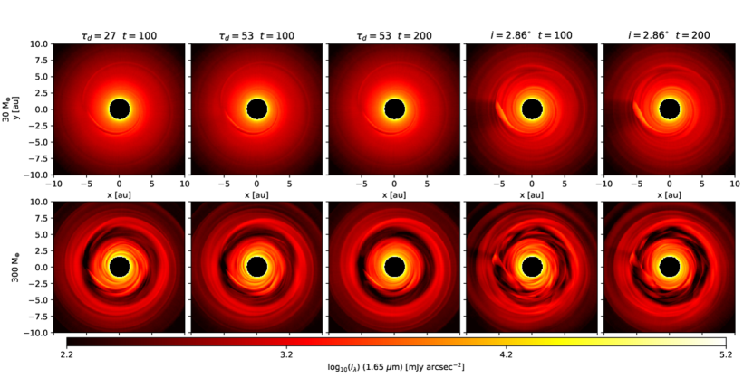
This is also true even in the case of the more massive planet. Whereas the disc feature resembling a possible protoplanet reveals itself in the sustained incline simulations as early as 100 orbits, there is no hint of this disc feature in any of the damped inclined simulations. In fact, the synthetic images of planets with damped orbits in Figure 15 much more closely resemble the $i=0^{\circ}$ 3D images in Figure 4 than the corresponding image of the sustained inclinations at $t=100$ and $t=200$ orbits.

It would seem that viscous protoplanetary discs are especially resilient to single-event or short term perturbations. If interactions with the host disc cause the orbits of slightly inclined isolated planets to damp to the midplane, the disruptive effects appear to be negligible on disc time-scales. If, however, a slightly inclined perturbation is sustained for any reason, it causes disruptions and features in near-IR observations which are not seen in surface density or midplane components of the disc. There are various known mechanisms that are capable of causing orbital inclination, such as the Kozai mechanism (Kozai, 1962), planet-planet scattering (e.g., Chatterjee et al., 2008), or mis-alignment of the disc itself (Bate, 2018). Even though simulations show that the orbital inclination of an isolated planet within a disc will damp towards the midplane, these simulations do not address what initially caused the inclination or whether that cause is capable of sustaining such an inclination.

While small inclinations could be quickly damped in a disc there are several mechanisms that could keep the inclination to a certain level. Masset & Velasco Romero (2017) found that small planets may have their inclinations excited from disc-planet interaction when considering how the planet’s luminosity heats its surrounding. Also the damping time is connected to the disc mass and viscosity, which are quite uncertain. Our $\alpha$-viscosity is well within the wide range of observed values (Rafikov, 2017), and was set at $\alpha=4\times 10^{-3}$ to help dampen out vertical shear instability (VSI). This value was obtained primarily using simulations with an aspect ratio of $H_{0}/R_{0}=0.05$ (Nelson et al., 2013). The time-scales for damping orbital inclination were also determined using this ratio for a planet at 5.2 au. Extending the orbital radius out to 30 au significantly lowers the effective gas density, changes the aspect ratio to $H_{0}/R_{0}\approx 0.07$. Any of these changes could impeded the disc’s ability to dampen the orbit of the planet.

As it is still unknown whether the inclination of planetary orbits, such as those seen in our own solar system, must be produced after the disc has dissipated, planet-disc orbital misalignment should not be dismissed as a potential cause of observed features in protoplanetary discs, and the effects of sustained inclination on the dynamics and observable features of these discs should continue to be investigated.

6 Summary & Conclusions

We ran two- and three-dimensional hydrodynamic simulations of viscous, vertically-isothermal, protoplanetary discs with an embedded 30 M_⊕ planet and a 300 M_⊕ planet at 5.2 au. For all simulations we use a constant $\alpha$-viscosity parameter of $\alpha=4.0\times 10^{-3}$. In the 3D cases we ran simulations in which the fixed orbit of the planets was aligned with the disc ($i=0^{\circ}$) and slightly misaligned with the disc ($i=2.86^{\circ}$), with and without damping the inclination over time. We post-processed each of these models using the Monte-Carlo radiation transfer code RADMC3D to created synthetic images which mimic how the features of these discs would be observed at effective H-band wavelengths (i.e., 1.65 µm).

Our results are summarized as follows:

1. In all models, the surface density evolution and the resultant features from the hydrodynamic simulations were effectively the same, regardless of whether the simulation was 2D or 3D, and regardless of whether the orbit was slightly inclined.

2. We found the $\tau_{s}=2/3$ surface for an unperturbed disc to be a full 3.3 thermal scale-heights above the midplane for our models, which means that observable features seen in H-band scattered-light images primarily come from the gas/dust dynamics that occur in the upper-atmosphere of the disc, and not from surface density or midplane effects. This emphasizes the need for 3D models, especially for disc models used to explain scattered light observations.

3. There are only slight differences in the features seen in scattered light images produced from the 2D300 and 3D300A models, and their average intensity profiles from these images are quite similar. We conclude that 2D simulations are adequate to model observable features of discs under the limitation of an embedded high-mass planet aligned with the disc midplane.

4. We find that inclined planets are able to “churn up” gas and dust material in the disc’s upper-atmosphere. The results are strong perturbations in the scattered light intensity that even include shadow-causing features. Disc features caused by inclined planets can be 10-20 times as bright as their surrounding areas. The model results also show dips in the average intensity profiles that could be falsely interpreted as the presence of a planet.

5. For a 300 M_⊕ planet which can clear out 94% of the material in its orbital path, the vertical optical depth to the disc midplane for H-band wavelengths is $\tau\approx 20$ at the orbital radius of the planet. We conclude that direct imaging of young planets embedded in the disc remains difficult to observe, even for massive planets in the gap.

6. A large-area shadowing of the disc (encompassing 30^∘ of the disc in our case), can possibly be detected by current instruments, even it remains difficult to trace back to its physical origin.

7. Certain features from embedded planets with a sustained orbital incline produce distinct non-axisymetric disc features in scattered light when observed from above or below, which again shows the importance of modeling both hemispheres of the disc.

Finally, we emphasize that for a sustained inclination, or any effect which would cause a significant continuous disruption in the evolution of the disc’s upper-atmosphere, fully 3D simulations are required to create scattered light models regardless of planet mass.

Appendix A RADMC3D Setup

To create synthetic scattered-light images from our hydrodynamic simulations as they would be observed in H-band wavelengths ($1.65\micron$), we apply, in post-processing, the well-tested Monte Carlo radiative transfer code RADMC3D v0.41 (Dullemond et al., 2012) to our results. We initially used the code to create a thermal structure of the dust embedded in the disc. Preliminary experiments indicated a surface around 3–4 thermal scale-heights above the midplane. We can therefor reasonably ignore larger grains which settle towards the midplane and assume a uniform dust-to-gas distribution of 0.01 for our purposes.

We model our radiative source as a star with a mass of $M_{*}=1M_{\sun}$, a radius of $R_{*}=2.6R_{\sun}$, an effective temperature of $T_{*}=4280$ K, and assume isotropic scattering. As the code requires values in centimeter-gram-second (cgs) units, we specified that the orbital radius of the planet was $R_{0}=5.2$ au, and the surface density at that radius was $\Sigma_{0}=75$ g cm^-2. This produces a disc with an initial mass of $M_{d}$ = 0.006 M_☉. This corresponds to a 0.08 M_☉ disc extended out to 100 au, consistent with observations (Andrews et al., 2009) and other simulations of protoplanetary discs (Flock et al., 2012; Dong & Fung, 2017a). We converted remaining values from the PLUTO simulations to cgs units using a unit length of $1\ell_{u}=5.2$ au, unit density $1\rho_{u}=M_{\sun}/\ell_{u}^{3}$, and a unit velocity of $1v_{u}=\sqrt{GM_{\sun}/\ell_{u}}/(2\pi)$, which corresponds to a unit time of one Keplerian orbit at $\mathbf{r}=(\ell_{u},\pi/2,\phi)$.

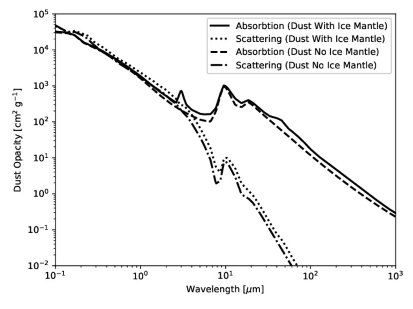
For the dust opacity we used the wavelength-dependent table by Preibisch et al. (1993), which is based on a grain size distribution of amorphous carbon and silicate grains, and is especially suited for the small grain sizes which are important for scattered-light image observations. For radiative transfer simulations on discs with an embedded planet at 5.2 au, we use opacity values for dust grains with no ice mantle, but for simulations scaled to approximate a simulation in which a planet is orbiting at 30 au, we use opacity values which include an ice mantle encasing the dust grains to reflect the lower temperatures at this distance (see Figure 16).

Figure 16: $\log_{10}-\log_{10}$ plot of the wavelength dependent opacities from Preibisch et al. (1993) used with RADMC3D to create temperature profiles and scattered light images from our hydrodynamic simulations of protoplanetary discs.

Once the thermal structure of the disc has been created we again use RADMC3D to create an image of our disc as it would be observed at 1.65 $\mu$m using second-order scattering, as well as calculating the height of the surface where the optical depth from an observer’s point a view is $\tau_{s}=2/3$. We refer to this as the observed surface throughout this paper.

Appendix B Lower Dust-to-Gas Ratio

We investigate the observable effect of diminished levels of small dust grains in the disc’s upper atmosphere by applying the RADMC3D code to the 3D simulations discussed in §3, but using a dust-to-gas ratio of $10^{-4}$ (we omitted making new synthetic images from the 2D simulations). The process of creating synthetic H-band images is otherwise identical to that described in Appendix A.

When we applied this process using the new dust-to-gas ratio, we found that the $\tau_{s}=2/3$ surface at $R=R_{0}$ for the unperturbed disc was only $1.5H$ above the midplane. Figure 17 shows the synthetic images produced from the 3D simulations involving 30 and 300 M_⊕ planets with inclined and aligned orbits. These images reveal disc features which are much closer to the midplane, and the observable disruptions from the inclined planets are not as apparent, and do not produce shadows (compare to Figure 4).

Figure 17: Synthetic H-band images from the 3D simulations involving 30 M_⊕ planets (Left), 300 M_⊕ planets (Right) with orbits with are aligned (Top) and mis-aligned (Bottom) with the disc, with the dust density reduced by a factor of 100 compared to those images seen in Figure 4. In this case the $\tau_{s}=2/3$ surface of an unperturbed disc is $1.5H$ above the midplane at $R=R_{0}$.

References

- Akiyama et al. (2015) Akiyama E., et al., 2015, ApJ, 802, L17
- Andrews et al. (2009) Andrews S. M., Wilner D. J., Hughes A. M., Qi C., Dullemond C. P., 2009, ApJ, 700, 1502
- Andrews et al. (2016) Andrews S. M., et al., 2016, ApJ, 820, L40
- Armitage (2011) Armitage P. J., 2011, ARA&A, 49, 195
- Arzamasskiy et al. (2018) Arzamasskiy L., Zhu Z., Stone J. M., 2018, MNRAS, 475, 3201
- Bae et al. (2016) Bae J., Zhu Z., Hartmann L., 2016, ApJ, 819, 134
- Bae et al. (2017) Bae J., Zhu Z., Hartmann L., 2017, ApJ, 850, 201
- Bate (2018) Bate M. R., 2018, MNRAS, 475, 5618
- Bate et al. (2003) Bate M. R., Lubow S. H., Ogilvie G. I., Miller K. A., 2003, MNRAS, 341, 213
- Benisty et al. (2015) Benisty M., et al., 2015, A&A, 578, L6
- Benisty et al. (2017) Benisty M., et al., 2017, A&A, 597, A42
- Bertrang et al. (2018) Bertrang G. H.-M., Avenhaus H., Casassus S., Montesinos M., Kirchschlager F., Perez S., Cieza L., Wolf S., 2018, MNRAS, 474, 5105
- Biller et al. (2014) Biller B. A., et al., 2014, ApJ, 792, L22
- Bitsch & Kley (2011) Bitsch B., Kley W., 2011, A&A, 530, A41
- Bitsch et al. (2013) Bitsch B., Crida A., Libert A.-S., Lega E., 2013, A&A, 555, A124
- Chametla et al. (2017) Chametla R. O., Sánchez-Salcedo F. J., Masset F. S., Hidalgo-Gámez A. M., 2017, MNRAS, 468, 4610
- Chatterjee et al. (2008) Chatterjee S., Ford E. B., Matsumura S., Rasio F. A., 2008, ApJ, 686, 580
- Chiang & Goldreich (1997) Chiang E. I., Goldreich P., 1997, ApJ, 490, 368
- Cresswell et al. (2007) Cresswell P., Dirksen G., Kley W., Nelson R. P., 2007, A&A, 473, 329
- Crida & Morbidelli (2007) Crida A., Morbidelli A., 2007, MNRAS, 377, 1324
- Crida et al. (2006) Crida A., Morbidelli A., Masset F., 2006, Icarus, 181, 587
- D’Alessio et al. (1998) D’Alessio P., Cantö J., Calvet N., Lizano S., 1998, ApJ, 500, 411
- Dong & Fung (2017a) Dong R., Fung J., 2017a, ApJ, 835, 38
- Dong & Fung (2017b) Dong R., Fung J., 2017b, ApJ, 835, 146
- Dong et al. (2015a) Dong R., Zhu Z., Rafikov R. R., Stone J. M., 2015a, ApJ, 809, L5
- Dong et al. (2015b) Dong R., Hall C., Rice K., Chiang E., 2015b, ApJ, 812, L32
- Dong et al. (2016) Dong R., Zhu Z., Fung J., Rafikov R., Chiang E., Wagner K., 2016, ApJ, 816, L12
- Dong et al. (2017) Dong R., Li S., Chiang E., Li H., 2017, ApJ, 843, 127
- Duffell & MacFadyen (2013) Duffell P. C., MacFadyen A. I., 2013, ApJ, 769, 41
- Dullemond et al. (2012) Dullemond C. P., Juhasz A., Pohl A., Sereshti F., Shetty R., Peters T., Commercon B., Flock M., 2012, RADMC-3D: A multi-purpose radiative transfer tool, Astrophysics Source Code Library (ascl:1202.015)
- Edgar & Quillen (2008) Edgar R. G., Quillen A. C., 2008, MNRAS, 387, 387
- Fedele et al. (2017) Fedele D., et al., 2017, A&A, 600, A72
- Flock et al. (2012) Flock M., Henning T., Klahr H., 2012, ApJ, 761, 95
- Flock et al. (2013) Flock M., Fromang S., González M., Commerçon B., 2013, A&A, 560, A43
- Fung & Chiang (2016) Fung J., Chiang E., 2016, ApJ, 832, 105
- Fung et al. (2014) Fung J., Shi J.-M., Chiang E., 2014, ApJ, 782, 88
- Garufi et al. (2013) Garufi A., et al., 2013, A&A, 560, A105
- Hunter (2007) Hunter J. D., 2007, Computing In Science & Engineering, 9, 90
- Juhász et al. (2015) Juhász A., Benisty M., Pohl A., Dullemond C. P., Dominik C., Paardekooper S.-J., 2015, MNRAS, 451, 1147
- Kanagawa et al. (2015a) Kanagawa K. D., Tanaka H., Muto T., Tanigawa T., Takeuchi T., 2015a, MNRAS, 448, 994
- Kanagawa et al. (2015b) Kanagawa K. D., Muto T., Tanaka H., Tanigawa T., Takeuchi T., Tsukagoshi T., Momose M., 2015b, ApJ, 806, L15
- Kenyon & Hartmann (1987) Kenyon S. J., Hartmann L., 1987, ApJ, 323, 714
- Keppler et al. (2018) Keppler M., et al., 2018, A&A, 617, A44
- Kley (2017) Kley W., 2017, preprint, (arXiv:1707.07148)
- Kley et al. (2012) Kley W., Müller T. W. A., Kolb S. M., Benítez-Llambay P., Masset F., 2012, A&A, 546, A99
- Kozai (1962) Kozai Y., 1962, AJ, 67, 591
- Marzari & Nelson (2009) Marzari F., Nelson A. F., 2009, ApJ, 705, 1575
- Masset & Velasco Romero (2017) Masset F. S., Velasco Romero D. A., 2017, MNRAS, 465, 3175
- Mignone et al. (2007) Mignone A., Bodo G., Massaglia S., Matsakos T., Tesileanu O., Zanni C., Ferrari A., 2007, ApJS, 170, 228
- Montesinos et al. (2016) Montesinos M., Perez S., Casassus S., Marino S., Cuadra J., Christiaens V., 2016, ApJ, 823, L8
- Müller et al. (2012) Müller T. W. A., Kley W., Meru F., 2012, A&A, 541, A123
- Müller et al. (2018) Müller A., et al., 2018, A&A, 617, L2
- Nelson et al. (2013) Nelson R. P., Gressel O., Umurhan O. M., 2013, MNRAS, 435, 2610
- Preibisch et al. (1993) Preibisch T., Ossenkopf V., Yorke H. W., Henning T., 1993, A&A, 279, 577
- Pringle (1981) Pringle J. E., 1981, ARA&A, 19, 137
- Rafikov (2017) Rafikov R. R., 2017, ApJ, 837, 163
- Reggiani et al. (2014) Reggiani M., et al., 2014, ApJ, 792, L23
- Ruge et al. (2014) Ruge J. P., Wolf S., Uribe A. L., Klahr H. H., 2014, A&A, 572, L2
- Shakura & Sunyaev (1973) Shakura N. I., Sunyaev R. A., 1973, A&A, 24, 337
- Sotiriadis et al. (2017) Sotiriadis S., Libert A.-S., Bitsch B., Crida A., 2017, A&A, 598, A70
- Stolker et al. (2016) Stolker T., et al., 2016, A&A, 595, A113
- Uribe et al. (2011) Uribe A. L., Klahr H., Flock M., Henning T., 2011, ApJ, 736, 85
- Varnière et al. (2004) Varnière P., Quillen A. C., Frank A., 2004, ApJ, 612, 1152
- Wagner et al. (2018) Wagner K., et al., 2018, ApJ, 854, 130
- Williams & Cieza (2011) Williams J. P., Cieza L. A., 2011, ARA&A, 49, 67
- Zhu (2019) Zhu Z., 2019, MNRAS, 483, 4221
- Zhu et al. (2014) Zhu Z., Stone J. M., Rafikov R. R., Bai X.-n., 2014, ApJ, 785, 122
- Zhu et al. (2015) Zhu Z., Dong R., Stone J. M., Rafikov R. R., 2015, ApJ, 813, 88
- de Val-Borro et al. (2006) de Val-Borro M., et al., 2006, MNRAS, 370, 529
- van Boekel et al. (2017) van Boekel R., et al., 2017, ApJ, 837, 132
- van der Marel et al. (2016) van der Marel N., Cazzoletti P., Pinilla P., Garufi A., 2016, ApJ, 832, 178