Adjoint-based methods for optimization and goal-oriented error control applied to fluid-structure interaction: implementation of a partition-of-unity dual-weighted residual estimator for stationary forward FSI problems in deal.II

Abstract

In this work, we implement goal-oriented error control and spatial mesh adaptivity for stationary fluid-structure interaction. The a posteriori error estimator is realized using the dual-weighted residual method in which the adjoint equation arises. The fluid-structure interaction problem is formulated within a variational-monolithic framework using arbitrary Lagrangian-Eulerian coordinates. The overall problem is nonlinear and solved with Newton’s method. We specifically consider the FSI-1 benchmark problem in which quantities of interest include the elastic beam displacements, drag, and lift. The implementation is provided open-source published on github https://github.com/tommeswick/goal-oriented-fsi. Possible extensions are discussed in the source code and in the conclusions of this paper.

1 Introduction

Fluid-structure interaction (FSI) is well-known [11, 25, 27, 10, 5, 8, 46, 26, 59] and a prime example of a multiphysics problem. It combines several challenges such as different types of partial-differential equations (PDE), interface-coupling, nonlinearities in the equations and due to coupling, Lagrangian and Eulerian coordinates. These result into typical numerical challenges such as robust spatial discretization (in particular for the moving interface), robust time-stepping schemes, efficient and robust linear and nonlinear solution algorithms. Computational work include different coupling concepts [37, 30, 53, 42, 16], space-time multiscale [51], reduced order modeling [24, 40, 52, 33], optimal control, parameter estimation, uncertainty quantification [41, 7, 48, 39, 21, 62], and efficient solver developments [34, 4, 28, 43, 13, 45, 15, 38, 55].

In this work, the main objective is the application and open-source implementation of goal-oriented a posteriori error control using the dual-weighted residual (DWR) method [6, 3]. For applications in fluid-structure interaction, we refer to [32, 23, 54, 57, 44, 46, 20, 22]. A recent overview of our own work using the adjoint FSI equation in goal-oriented error estimation and optimization was done in [60]. In [49] a variational localization using a partition-of-unity (PU) was proposed, facilitating the application to coupled problems such as fluid-structure interaction. In view of increasing initiatives of open-source developments, another purpose of this work is to provide a documented open-source code. To this end, a stationary fluid-structure interaction problem is considered in order to explain the main steps of a PU-DWR estimator. The problem is formulated within a monolithic framework using arbitrary Lagrangian-Eulerian (ALE) coordinates. For some well-posedness results of such stationary FSI problems, we refer to [31, 61]. Together with the goal functional under consideration, the FSI formulation serves as PDE constraint and the Lagrange formalism can be applied. Specifically, the monolithic formulation yields a consistent adjoint equation.

For the monolithic, stationary, FSI formulation we follow [47, 56] and for the PU-DWR error estimator, we follow [49]. The basis of our programming code is [58] (see also updates on github) and we take some ideas from deal.II [1, 2] step-14. Our resulting code can be found on github.

2 Variational-monolithic ALE fluid-structure interaction

2.1 Modeling

For the function spaces in the (fixed) reference domains $\widehat{\Omega},\widehat{\Omega}_{f},\widehat{\Omega}_{s}$, we define ${\widehat{V}}:=H^{1}(\widehat{\Omega})^{d}.$ In the fluid and solid domains, we define further:

$${\widehat{L}}_{f} :=L^{2}(\widehat{\Omega}_{f}),\quad{\widehat{L}}_{f}^{0}:=L^{2}(\widehat{\Omega}_{f})/\mathbb{R},\quad{\widehat{V}}_{f}^{0}:=\{{\widehat{v}}_{f}\in H^{1}(\widehat{\Omega}_{f})^{d}:\,{\widehat{v}}_{f}=0\text{ on }\widehat{\Gamma}_{\text{in}}\cup\widehat{\Gamma}_{D}\},$$

$${\widehat{V}}_{f,{\widehat{u}}}^{0} :=\{{\widehat{u}}_{f}\in H^{1}(\widehat{\Omega}_{f})^{d}:\,{\widehat{u}}_{f}={\widehat{u}}_{s}\text{ on }\widehat{\Gamma}_{i},\quad{\widehat{u}}_{f}=0\text{ on }\widehat{\Gamma}_{\text{in}}\cup\widehat{\Gamma}_{D}\cup\widehat{\Gamma}_{\text{out}}\},$$

$${\widehat{V}}_{f,{\widehat{u}},\widehat{\Gamma}_{i}}^{0} :=\{{\widehat{\psi}}_{f}\in H^{1}(\widehat{\Omega}_{f})^{d}:\,{\widehat{\psi}}_{f}=0\text{ on }\widehat{\Gamma}_{i}\cup\widehat{\Gamma}_{\text{in}}\cup\widehat{\Gamma}_{D}\cup\widehat{\Gamma}_{\text{out}}\},$$

$${\widehat{V}}_{s}^{0} :=\{{\widehat{u}}_{s}\in H^{1}(\widehat{\Omega}_{s})^{d}:\,{\widehat{u}}_{s}=0\text{ on }\widehat{\Gamma}_{D}\}.$$

As stationary FSI problem in variational-monolithic ALE form, we have [56][p. 29]:

Problem 2.1.

Find $\{{\widehat{v}}_{f},{\widehat{u}}_{f},{\widehat{u}}_{s},{\widehat{p}}_{f}\}\in\{{\widehat{v}}_{f}^{D}+{\widehat{V}}_{f,{\widehat{v}}}^{0}\}\times\{{\widehat{u}}_{f}^{D}+{\widehat{V}}_{f,{\widehat{u}}}^{0}\}\times\{{\widehat{u}}_{s}^{D}+{\widehat{V}}_{s}^{0}\}\times{\widehat{L}}_{f}^{0}$, such that

$$\begin{aligned} ({\widehat{\rho}}_{f}\widehat{J}({\widehat{F}}^{-1}{\widehat{v}}_{f}\cdot{\widehat{\nabla}}){\widehat{v}}_{f}),{\widehat{\psi}}^{v})_{\widehat{\Omega}_{f}}&\\ +(\widehat{J}{\widehat{\sigma}}_{f}{\widehat{F}}^{-T},{\widehat{\nabla}}{\widehat{\psi}}^{v})_{\widehat{\Omega}_{f}}-\langle{\widehat{g}}_{f},{\widehat{\psi}}^{v}\rangle_{\widehat{\Gamma}_{N}}-({\widehat{\rho}}_{f}\widehat{J}{\widehat{f}}_{f},{\widehat{\psi}}^{v})_{\widehat{\Omega}_{f}}&=0&&\forall{\widehat{\psi}}^{v}\in{\widehat{V}}_{f,{\widehat{v}}}^{0},\\ ({\widehat{F}}{\widehat{\Sigma}},{\widehat{\nabla}}{\widehat{\psi}}^{v})_{\widehat{\Omega}_{s}}-({\widehat{\rho}}_{s}{\widehat{f}}_{s},{\widehat{\psi}}^{v})_{\widehat{\Omega}_{s}}&=0&&\forall{\widehat{\psi}}^{v}\in{\widehat{V}}_{s}^{0},\\ ({\widehat{\sigma}}_{\text{mesh}},{\widehat{\nabla}}{\widehat{\psi}}^{u})_{\widehat{\Omega}_{f}}+({\widehat{v}}_{s},{\widehat{\psi}}^{u})_{\widehat{\Omega}_{s}}&=0&&\forall{\widehat{\psi}}^{u}\in{\widehat{V}}_{f,{\widehat{u}},\widehat{\Gamma}_{i}}^{0},\\ (\widehat{\operatorname{div}}\,(\widehat{J}{\widehat{F}}^{-1}{\widehat{v}}_{f}),{\widehat{\psi}}^{p})_{\widehat{\Omega}_{f}}&=0&&\forall{\widehat{\psi}}^{p}\in{\widehat{L}}_{f}^{0},\end{aligned}$$

with ${\widehat{F}}=\widehat{I}+{\widehat{\nabla}}{\widehat{u}},\widehat{J}=det({\widehat{F}}),{\widehat{\sigma}}_{f}=-{\widehat{p}}_{f}\widehat{I}+{\widehat{\rho}}_{f}\nu_{f}({\widehat{\nabla}}{\widehat{v}}_{f}{\widehat{F}}^{-1}+{\widehat{F}}^{-T}{\widehat{\nabla}}{\widehat{v}}_{f}),{\widehat{\Sigma}}=2\mu_{s}{\widehat{E}}+\lambda_{s}tr({\widehat{E}})\widehat{I},{\widehat{E}}=0.5({\widehat{F}}^{T}{\widehat{F}}-\widehat{I}),{\widehat{\sigma}}_{\text{mesh}}=\alpha_{u}{\widehat{\nabla}}{\widehat{u}}_{f}$, volume forces ${\widehat{f}}_{f}$ and ${\widehat{f}}_{s}$ (both zero in this work), flow correction term ${\widehat{g}}_{f}$ (do-nothing [35]), densities ${\widehat{\rho}}_{s},{\widehat{\rho}}_{f}$, kinematic viscosity $\nu_{f}$, and the Lamé parameters $\mu_{s},\lambda_{s}$. All explanations are provided in [56][Chapter 3].

2.2 Discretization and numerical solution

For spatial discretization, a conforming Galerkin finite element scheme on quadrilateral mesh elements is employed [12]. Specifically, we use $Q_{2}^{c}$ elements for ${\widehat{v}}$ and ${\widehat{u}}:={\widehat{u}}_{f}+{\widehat{u}}_{s}$, and $Q_{1}^{c}$ elements for ${\widehat{p}}$. For the flow problem $({\widehat{v}},{\widehat{p}})$, this is the well-known inf-sup stable Taylor-Hood element; see e.g., [29]. Due to variational-monolithic coupling and globally-defined finite elements, the fluid pressure must be extended to the solid domain, which is achieved via $\alpha_{u}[({\widehat{\nabla}}{\widehat{p}}_{s},{\widehat{\nabla}}{\widehat{\psi}}^{p})+({\widehat{p}}_{s},{\widehat{\psi}}^{p})]$, and $\alpha_{u}$ (as before) small, positive. This is only for convenience, an alternative is to work with the FE_NOTHING element in deal.II. The nonlinear problem is solved with Newton’s method. Therein, for simplicity in this work, we utilize a sparse direct solver [14]. For algorithmic descriptions of our implementation, we refer to [56].

3 PU-DWR goal-oriented error control

The Galerkin approximation reads: Find ${\widehat{U}}_{h}=\{{\widehat{v}}_{f,h},{\widehat{u}}_{f,h},{\widehat{u}}_{s,h},{\widehat{p}}_{f,h}\}\in{\widehat{X}}^{0}_{h,D}$, where ${\widehat{X}}_{h,D}^{0}:=\{{\widehat{v}}_{f,h}^{D}+{\widehat{V}}_{f,{\widehat{v}},h}^{0}\}\times\{{\widehat{u}}_{f,h}^{D}+{\widehat{V}}_{f,{\widehat{u}},h}^{0}\}\times\{{\widehat{u}}_{s,h}^{D}+{\widehat{V}}_{s,h}^{0}\}\times{\widehat{L}}_{f,h}^{0}$, such that

$$\hat{A}({\widehat{U}}_{h})({\widehat{\Psi}}_{h})=\hat{F}({\widehat{\Psi}}_{h})\quad\forall{\widehat{\Psi}}_{h}\in{\widehat{X}}_{h},$$ (1)

where ${\widehat{X}}_{h}$ is the test space with homogeneous Dirichlet conditions.

3.1 Goal functional

The solution ${\widehat{U}}_{h}$ is used to calculate an approximation $J({\widehat{U}}_{h})$ of the goal-functional $J({\widehat{U}}):{\widehat{X}}\rightarrow\mathbb{R}$. This functional is assumed to be sufficiently differentiable. The drag value as goal functional reads

$$J({\widehat{U}}):=\int_{\hat{S}}\widehat{J}{\widehat{\sigma}}_{f}{\widehat{F}}^{-T}{\widehat{n}}_{f}\,{\widehat{d}}\,\text{d}{\widehat{s}},$$

where ${\widehat{n}}_{f}$ is the outward point normal vector of the cylinder boundary $\hat{S}$ [36] and the FSI interface $\widehat{\Gamma}_{i}$. Moreover, ${\widehat{d}}$ is a unit vector perpendicular to the mean flow direction. For the drag, we use ${\widehat{d}}=(1,0)$.

3.2 Error representation

We use the (formal) Euler-Lagrange method, to derive a computable representation of the approximation error $J({\widehat{U}})-J({\widehat{U}}_{h})$. The task is: Find ${\widehat{U}}\in{\widehat{X}}^{0}_{D}$ such that

$$\min\{J({\widehat{U}})-J({\widehat{U}}_{h})\}\quad\text{s.t. }{\widehat{A}}({\widehat{U}})({\widehat{\Psi}})=\hat{F}({\widehat{\Psi}})\quad\forall{\widehat{\Psi}}\in{\widehat{X}},$$

from which we obtain the optimality system

$${\cal L}^{\prime}_{{\widehat{Z}}}({\widehat{U}},{\widehat{Z}})(\delta{\widehat{Z}}) ={\widehat{F}}(\delta{\widehat{Z}})-{\widehat{A}}({\widehat{U}})(\delta{\widehat{Z}})=0\quad\forall\delta{\widehat{Z}}\in{\widehat{X}},\quad\text{(Primal problem)},$$

$${\cal L}^{\prime}_{{\widehat{U}}}({\widehat{U}},{\widehat{Z}})(\delta{\widehat{U}}) =J^{\prime}({\widehat{U}})(\delta{\widehat{U}})-{\widehat{A}}^{\prime}_{{\widehat{U}}}({\widehat{U}})(\delta{\widehat{U}},{\widehat{Z}})=0\quad\forall\delta{\widehat{U}}\in{\widehat{X}},\quad\text{(Adjoint problem)}.$$

Using the main theorem from [6], we obtain:

Theorem 3.1.

We have the error identity:

$$J({\widehat{U}})-J({\widehat{U}}_{h})=\frac{1}{2}\rho({\widehat{U}}_{h})({\widehat{Z}}-{\widehat{\Phi}}_{h})+\frac{1}{2}\rho^{*}({\widehat{U}}_{h},{\widehat{Z}}_{h})({\widehat{U}}-{\widehat{\Psi}}_{h})+{\cal R}^{(3)}_{h},$$ (2)

for all $\{{\widehat{\Psi}}_{h},{\widehat{\Phi}}_{h}\}\in{\widehat{X}}_{h}\times{\widehat{X}}_{h}$ and with the primal and adjoint residuals:

$$\rho({\widehat{U}}_{h})({\widehat{Z}}-{\widehat{\Phi}}_{h}) :=-A({\widehat{U}}_{h})(\cdot)+\hat{F}(\cdot),$$

$$\rho^{*}({\widehat{U}}_{h},{\widehat{Z}}_{h})({\widehat{U}}-{\widehat{\Psi}}_{h}) :=J^{\prime}({\widehat{U}}_{h})(\cdot)-A^{\prime}({\widehat{U}}_{h})(\cdot,{\widehat{Z}}_{h})+\hat{F}(\cdot).$$

The remainder term is ${\cal R}^{(3)}_{h}$ is of cubic order. This error identity can be used to define the error estimator $\eta$, which can be further utilized to design adaptive schemes.

Corollary 3.2 (Primal error).

The primal error identity reads:

$$J({\widehat{U}})-J({\widehat{U}}_{h})=\rho({\widehat{U}}_{h})({\widehat{Z}}-{\widehat{\Phi}}_{h})+{\cal R}^{(2)}_{h}.$$ (3)

3.3 Adjoint equation, discretization, and numerical solution

The adjoint equation reads: Find ${\widehat{Z}}=({\widehat{z}}^{v},{\widehat{z}}^{u},{\widehat{z}}^{p})\in{\widehat{X}}$ such that

$$J^{\prime}({\widehat{U}})({\widehat{\Phi}})={\widehat{A}}^{\prime}_{{\widehat{U}}}({\widehat{U}})({\widehat{\Phi}},{\widehat{Z}})\quad\forall{\widehat{\Phi}}\in{\widehat{X}},$$

and the explicit form can be found in [56, 60].

For the discretization, we briefly mention that higher-order information for the adjoint solution must be employed due to Galerkin orthogonality; in this work ${\widehat{X}}_{h}\subset{\widehat{X}}_{h}^{(2)}\subset{\widehat{X}}$. For simplicity, this is realized with global-higher order finite elements and in order to ensure again inf-sup stability, we use $Q_{4}^{c}$ elements for ${\widehat{z}}^{v}$ and ${\widehat{z}}^{u}$, and $Q_{2}^{c}$ elements for ${\widehat{z}}^{p}$. It is clear that this is an expensive choice. For the numerical solution, the same solvers as for the primal problem are taken (see Section 2.2), namely a Newton-type method and sparse direct solver. Since the adjoint problem is linear, Newton’s method converges in one step. This is a trivial information, but for debugging reasons useful.

3.4 Localization

A PU localization [49] for stationary FSI reads:

Proposition 3.1.

We have for the primal error part $\rho({\widehat{U}}_{h})(\cdot)$ the a posteriori error estimate

$$|J({\widehat{U}})-J({\widehat{U}}_{h})|\leq\eta:=\bigl{|}\sum_{i=1}^{M}\eta_{i}\bigr{|}\leq\sum_{i=1}^{M}|\eta_{i}|$$ (4)

where $M$ is the dimension of the PU finite element space ${\widehat{V}}_{PU}$ (composed of $Q_{1}^{c}$ functions $\chi_{i}$) and with the PU-DoF indicators

$$\eta_{i} =-A({\widehat{U}}_{h})(({\widehat{Z}}_{h}^{(2)}-i_{h}{\widehat{Z}}_{h}^{(2)}){\widehat{\Psi}}_{i})+\hat{F}(({\widehat{Z}}_{h}^{(2)}-i_{h}{\widehat{Z}}_{h}^{(2)}){\widehat{\Psi}}_{i})$$

$$=-({\widehat{\rho}}_{f}\widehat{J}({\widehat{F}}^{-1}{\widehat{v}}_{f}\cdot{\widehat{\nabla}}){\widehat{v}}_{f}),{\widehat{\psi}}_{i}^{v})_{\widehat{\Omega}_{f}}-(\widehat{J}{\widehat{\sigma}}_{f}{\widehat{F}}^{-T},{\widehat{\nabla}}{\widehat{\psi}}_{i}^{v})_{\widehat{\Omega}_{f}}+\langle{\widehat{g}}_{f},{\widehat{\psi}}_{i}^{v}\rangle_{\widehat{\Gamma}_{N}}$$

$$\quad-({\widehat{F}}{\widehat{\Sigma}},{\widehat{\nabla}}{\widehat{\psi}}_{i}^{v})_{\widehat{\Omega}_{s}}-({\widehat{\sigma}}_{\text{mesh}},{\widehat{\nabla}}{\widehat{\psi}}_{i}^{u})_{\widehat{\Omega}_{f}}-(\widehat{\operatorname{div}}\,(\widehat{J}{\widehat{F}}^{-1}{\widehat{v}}_{f}),{\widehat{\psi}}_{i}^{p})_{\widehat{\Omega}_{f}}$$

$$\quad+({\widehat{\rho}}_{f}\widehat{J}{\widehat{f}}_{f},{\widehat{\psi}}_{i}^{v})_{\widehat{\Omega}_{f}}+({\widehat{\rho}}_{s}{\widehat{f}}_{s},{\widehat{\psi}}_{i}^{v})_{\widehat{\Omega}_{s}}$$

with the interpolation $i_{h}:{\widehat{X}}_{h}^{(2)}\to{\widehat{X}}_{h}$ and the weighting functions are defined as

$${\widehat{\psi}}_{i}^{v} :=(\phi_{2h,v}^{(2)}-\phi_{h,v})\chi_{i},\quad{\widehat{\psi}}_{i}^{u}:=(\phi_{2h,u}^{(2)}-\phi_{h,u})\chi_{i},\quad{\widehat{\psi}}_{i}^{p}:=(\phi_{2h,p}^{(2)}-\phi_{h,p})\chi_{i}.$$

3.5 Adaptive algorithm

1. Compute the primal solution ${\widehat{U}}_{h}$ and the (higher-order) adjoint solution ${\widehat{Z}}_{h}^{(2)}$ on the present mesh $\mathcal{T}_{h}$.

2. Evaluate $|\eta|:=|\sum_{i}\eta_{i}|$ in (4).

3. Check, if the stopping criterion is satisfied: $|J({\widehat{U}})-J({\widehat{U}}_{h})|\leq|\eta|\leq TOL$, then accept $U_{h}$ within the tolerance $TOL$. Otherwise, proceed to the following step.

4. Mark all elements $K_{i}$ for refinement that touch DoFs $i$ with indicator $\eta_{i}$ with $\eta_{i}\geq\frac{\alpha\eta}{M_{el}}$ (where $M_{el}$ denotes the total number of elements of the mesh $\mathcal{T}_{h}$ and $\alpha\approx 1$).
   Alternatively, pure DoF-based refinement in $i$ can be carried out.

4 Numerical tests

In this section, we consider the FSI-1 benchmark [36] (see also the books [11, 10] and our own former results [47, 58]) and the 2D-1 benchmark [50]. The drag value is taken as goal functional. As previously mentioned, this paper is accompanied with a respective open-source implementation on github based on the finite element library deal.II [1, 2] and our previous fluid-structure interaction code [58], which is also available on github.

4.1 FSI-1 benchmark

The configuration, all parameters, and reference values can be found in [36]. The reference value for computing the true error was computed on a five times refined mesh and is $1.5370185576528707e+01$ (see also in the provided github code). Our results from the file dwr_results.txt are:

Dofs    True err     Est err      Est ind      Eff          Ind
13310   2.58e-01     1.43e-01     4.37e-01     5.54e-01     1.69e+00
20921   9.00e-02     4.75e-02     1.60e-01     5.28e-01     1.77e+00
37874   3.20e-02     1.09e-02     5.96e-02     3.40e-01     1.86e+00
68754   1.84e-02     4.57e-03     2.77e-02     2.48e-01     1.51e+00

Furthermore, the terminal output yields

DisX  :     2.2656126465725842e-05
DisY  :     8.1965770448936843e-04
P-Diff:     1.4819455817646477e+02
P-front:    1.4819455817646477e+02
------------------
Face drag:      1.5351806985399641e+01
Face lift:      7.3933527637991259e-01

where Face drag represents the chosen goal functional. While the error reductions in the True err $J({\widehat{U}})-J({\widehat{U}}_{h})$ and the estimated error $\eta$ are reasonable, the effectivity index Eff has room for improvement. The indicator index Ind (for the definition see [49]) performs quite well. The main reason for the intermediate effectivity indices might be the accuracy of the reference value. Second, we notice that only the primal error part $\rho$ (Corollary 3.2) was used. As shown in our recent studies for quasi-linear problems, the adjoint error part $\rho^{*}$ might play a crucial role in order to obtain nearly perfect effectivity indices for highly nonlinear problems [18]. Graphical solutions of the primal solution, including the adaptively refined mesh, and the adjoint solution are displayed in Figure 1.

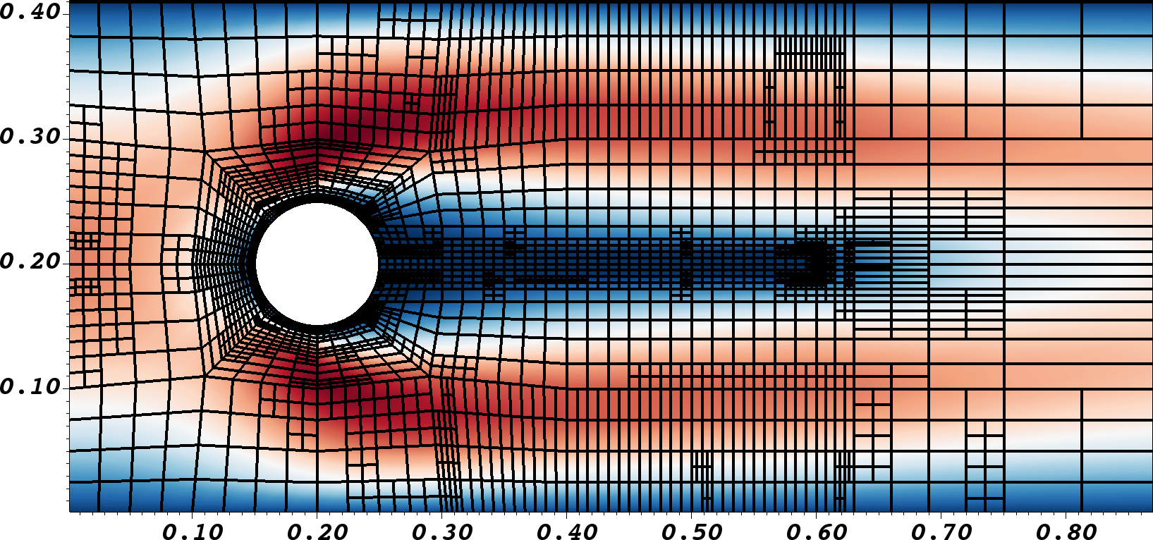
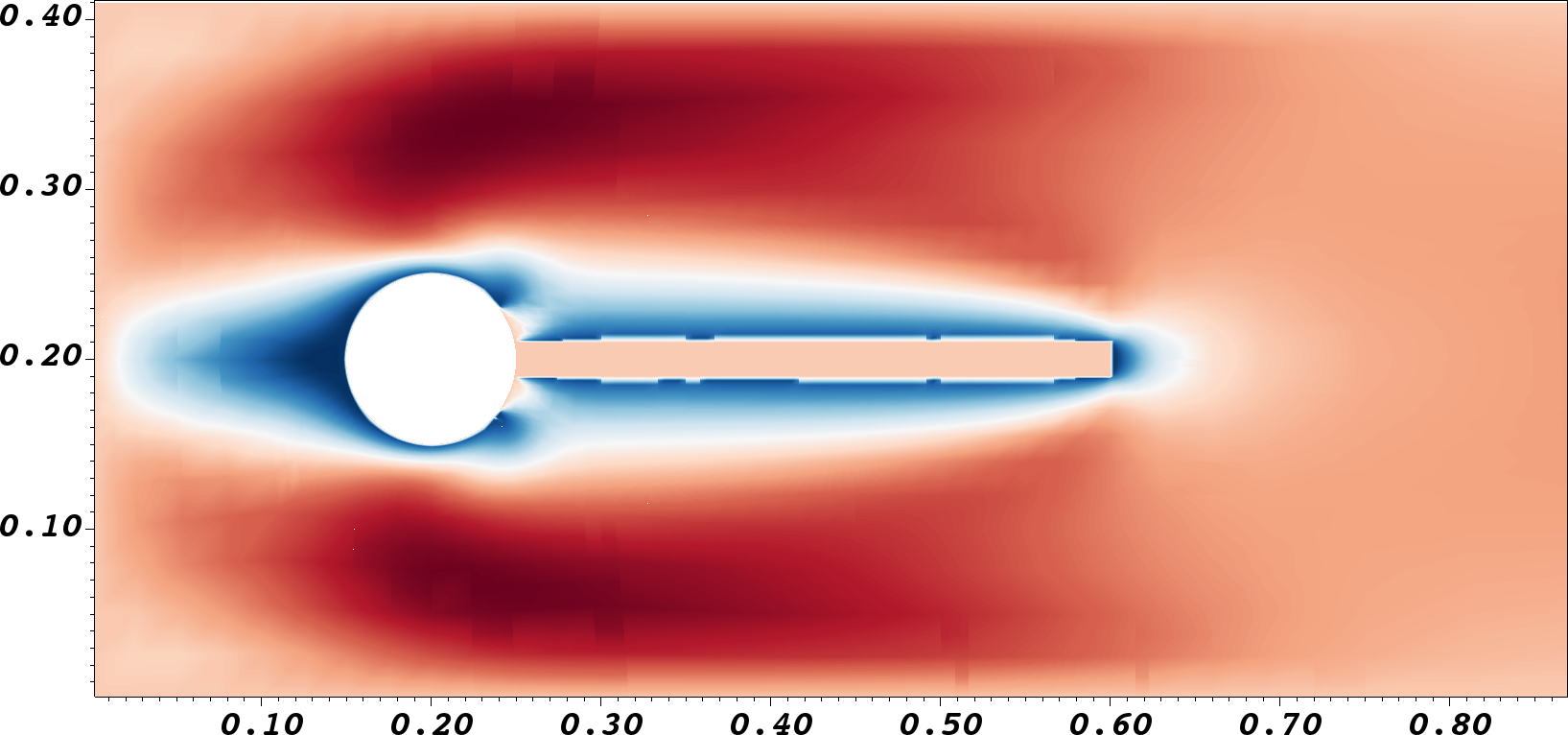
Figure 1: FSI-1 benchmark: Primal solution of ${\widehat{v}}_{x}$ and adjoint solution ${\widehat{z}}^{v_{x}}$. The adaptive mesh is displayed together with the primal solution (right).

4.2 Adaptation to flow benchmark 2D-1

The provided code can be adapted with minimal changes to the 1996 flow around cylinder benchmark 2D-1 [50]. In the *.inp file the material ids for solid must be set to $0$ (flow), and the inflow and material parameters are adapted correspondingly. Of course, in this code, the displacement variables are still computed despite that they are zero everywhere, which increases the computational cost in comparison to a pure fluid flow code. Due to the zero displacements ${\widehat{u}}=0$, the ALE mapping is the identity, yielding ${\widehat{F}}=\widehat{I}$ and $det({\widehat{F}})=1$. Consequently, there is no mesh deformation and the Navier-Stokes equations fully remain in Eulerian coordinates. Here, extracting information from dwr_results.txt, the findings for the drag value as goal functional are:

Dofs    True err    Est err      Est ind      Eff          Ind
1610    3.51e-01    2.97e-01     6.20e-01     8.44e-01     1.76e+00
2586    8.80e-02    7.27e-02     2.21e-01     8.26e-01     2.51e+00
4764    1.89e-02    1.54e-02     7.11e-02     8.14e-01     3.75e+00
10830   3.23e-03    2.95e-03     1.82e-02     9.13e-01     5.62e+00

The pressure, drag (goal functional), and lift values are taken from the terminal output:

P-Diff:     1.1743527755157424e-01
P-front:    1.3213237901562136e-01
P-back:     1.4697101464047121e-02
------------------
Face drag:      5.5754969431700365e+00
Face lift:      1.0717678080199560e-02

These values fit well with the reference values given in [50]. Moreover, we observe very stable effectivity indices, which indicate that the primal error estimator $\rho$ (Corollary 3.2) is for incompressible Navier-Stokes a sufficient choice. Indeed, using this part only, was already suggested in early work [6, 9]. Finally, we notice that extensions to multiple goal functionals for the 2D-1 benchmark were undertaken in [17, 19].

5 Conclusions

In this work, we developed and implemented PU-DWR goal-oriented error control and spatial mesh adaptivity for stationary fluid-structure interaction. An important part is the open-source programming code published on github. As numerical example, the FSI-1 benchmark is chosen. Therein, mesh adaptivity performs as expected and also the error reductions in the true error and estimated error are good. However, the effectivity index may be improved. Extensions of this work include inter alia the implementation of the adjoint error part $\rho^{*}$, local-higher order interpolations for the adjoint rather than using global-higher order finite elements, parallel iterative/multigrid linear solvers within Newton’s method, and a 3D implementation. The latter is implementation-wise not difficult with deal.II’s dimension-independent programming, but the linear solver becomes really important.

6 Acknowledgments

This work is supported by the Deutsche Forschungsgemeinschaft (DFG) under Germany’s Excellence Strategy within the cluster of Excellence PhoenixD (EXC 2122, Project ID 390833453).

References

- [1] D. Arndt, W. Bangerth, T. C. Clevenger, D. Davydov, M. Fehling, D. Garcia-Sanchez, G. Harper, T. Heister, L. Heltai, M. Kronbichler, R. M. Kynch, M. Maier, J.-P. Pelteret, B. Turcksin, and D. Wells. The deal.II library, version 9.1. Journal of Numerical Mathematics, 27:203–213, 2019.
- [2] D. Arndt, W. Bangerth, D. Davydov, T. Heister, L. Heltai, M. Kronbichler, M. Maier, J.-P. Pelteret, B. Turcksin, and D. Wells. The deal.ii finite element library: Design, features, and insights. Computers & Mathematics with Applications, 2020.
- [3] W. Bangerth and R. Rannacher. Adaptive Finite Element Methods for Differential Equations. Birkhäuser, Lectures in Mathematics, ETH Zürich, 2003.
- [4] A. T. Barker and X.-C. Cai. Scalable parallel methods for monolithic coupling in fluid-structure interaction with application to blood flow modeling. Journal of Computational Physics, 229(3):642 – 659, 2010.
- [5] Y. Bazilevs, K. Takizawa, and T. Tezduyar. Computational Fluid-Structure Interaction: Methods and Applications. Wiley, 2013.
- [6] R. Becker and R. Rannacher. An optimal control approach to a posteriori error estimation in finite element methods. Acta Numerica, Cambridge University Press, pages 1–102, 2001.
- [7] C. Bertoglio, P. Moireau, and J. Gerbeau. Sequential parameter estimation in fluid-structure problems. application to hemodynamics. Int. J. Numer. Meth. Biomed. Engrg., 28:434–455, 2012.
- [8] T. Bodnár, G. Galdi, and Š. Nečasová. Fluid-Structure Interaction and Biomedical Applications. Advances in Mathematical Fluid Mechanics. Springer Basel, 2014.
- [9] M. Braack and T. Richter. Solutions of 3d navier–stokes benchmark problems with adaptive finite elements. Computers & Fluids, 35(4):372 – 392, 2006.
- [10] H.-J. Bungartz, M. Mehl, and M. Schäfer. Fluid-Structure Interaction II: Modelling, Simulation, Optimization. Lecture Notes in Computational Science and Engineering. Springer, 2010.
- [11] H.-J. Bungartz and M. Schäfer. Fluid-Structure Interaction: Modelling, Simulation, Optimization, volume 53 of Lecture Notes in Computational Science and Engineering. Springer, 2006.
- [12] P. G. Ciarlet. The finite element method for elliptic problems. North-Holland, Amsterdam [u.a.], 2. pr. edition, 1987.
- [13] P. Crosetto, S. Deparis, G. Fourestey, and A. Quarteroni. Parallel algorithms for fluid-structure interaction problems in haemodynamics. SIAM J. Sci. Comp., 33(4):1598–1622, 2011.
- [14] T. A. Davis and I. S. Duff. An unsymmetric-pattern multifrontal method for sparse LU factorization. SIAM J. Matrix Anal. Appl., 18(1):140–158, 1997.
- [15] S. Deparis, D. Forti, G. Grandperrin, and A. Quarteroni. Facsi: A block parallel preconditioner for fluid-structure interaction in hemodynamics. Journal of Computational Physics, 327:700–718, 2016.
- [16] T. Dunne. An Eulerian approach to fluid-structure interaction and goal-oriented mesh adaption. Int. J. Numer. Methods in Fluids, 51:1017–1039, 2006.
- [17] B. Endtmayer, U. Langer, J. P. Thiele, and T. Wick. Hierarchical DWR Error Estimates for the Navier Stokes Equation: and Enrichment, 2019.
- [18] B. Endtmayer, U. Langer, and T. Wick. Multigoal-Oriented Error Estimates for Non-linear Problems. Journal of Numerical Mathematics, 27(4):215–236, 2019.
- [19] B. Endtmayer, U. Langer, and T. Wick. Two-Side a Posteriori Error Estimates for the Dual-Weighted Residual Method. SIAM J. Sci. Comput., 42(1):A371–A394, 2020.
- [20] L. Failer. Optimal Control of Time-Dependent Nonlinear Fluid-Structure Interaction. PhD thesis, Technical University Munich, 2017.
- [21] L. Failer and T. Richter. A newton multigrid framework for optimal control of fluid–structure interactions. Optimization and Engineering, 2020.
- [22] L. Failer and T. Wick. Adaptive time-step control for nonlinear fluid-structure interaction. Journal of Computational Physics, 366:448 – 477, 2018.
- [23] P. Fick, E. Brummelen, and K. Zee. On the adjoint-consistent formulation of interface conditions in goal-oriented error estimation and adaptivity for fluid-structure interaction. Computer Methods in Applied Mechanics and Engineering, 199:3369–3385, 2010.
- [24] L. Formaggia, J.-F. Gerbeau, F. Nobile, and A. Quarteroni. On the coupling of 3d and 1d Navier-Stokes equations for flow problems in compliant vessels. Comp. Methods Appl. Mech. Engig, 191:561–582, 2001.
- [25] L. Formaggia, A. Quarteroni, and A. Veneziani. Cardiovascular Mathematics: Modeling and simulation of the circulatory system. Springer-Verlag, Italia, Milano, 2009.
- [26] S. Frei, B. Holm, T. Richter, T. Wick, and H. Yang. Fluid-structure interactions: Fluid-Structure Interaction: Modeling, Adaptive Discretisations and Solvers. de Gruyter, 2017.
- [27] G. Galdi and R. Rannacher. Fundamental Trends in Fluid-Structure Interaction. World Scientific, 2010.
- [28] M. Gee, U. Küttler, and W. Wall. Truly monolithic algebraic multigrid for fluid–structure interaction. Int. J. Numer. Meth. Engrg., 85(8):987–1016, 2011.
- [29] V. Girault and P.-A. Raviart. Finite Element method for the Navier-Stokes equations. Number 5 in Computer Series in Computational Mathematics. Springer-Verlag, 1986.
- [30] R. Glowinski, T. Pan, T. Hesla, D. Joseph, and J. Périaux. A fictitious domain approach to the direct numerical simulation of incompressible viscous flow past moving rigid bodies: Application to particulate flow. Journal of Computational Physics, 169(2):363 – 426, 2001.
- [31] C. Grandmont. Existence for a three-dimensional steady state fluid-structure interaction problem. Journal of Mathematical Fluid Mechanics, 4:76–94, 2002.
- [32] T. Grätsch and K.-J. Bathe. Goal-oriented error estimation in the analysis of fluid flows with structural interactions. Comp. Methods Appl. Mech. Engrg., 195:5673–5684, 2006.
- [33] N. Hagmeyer, M. Mayr, I. Steinbrecher, and A. Popp. Fluid-beam interaction: Capturing the effect of embedded slender bodies on global fluid flow and vice versa, 2021.
- [34] M. Heil. An efficient solver for the fully coupled solution of large-displacement fluid-structure interaction problems. Comput. Methods Appl. Mech. Engrg., 193:1–23, 2004.
- [35] J. G. Heywood, R. Rannacher, and S. Turek. Artificial boundaries and flux and pressure conditions for the incompressible Navier-Stokes equations. International Journal of Numerical Methods in Fluids, 22:325–352, 1996.
- [36] J. Hron and S. Turek. Proposal for numerical benchmarking of fluid-structure interaction between an elastic object and laminar incompressible flow, volume 53, pages 146 – 170. Springer-Verlag, 2006.
- [37] T. Hughes, W. Liu, and T. Zimmermann. Lagrangian-Eulerian finite element formulation for incompressible viscous flows. Comput. Methods Appl. Mech. Engrg., 29:329–349, 1981.
- [38] D. Jodlbauer, U. Langer, and T. Wick. Parallel block-preconditioned monolithic solvers for fluid-structure interaction problems. Int. J. Num. Meth. Eng., 117(6):623–643, 2019.
- [39] J. Kratzke. Uncertainty Quantification for Fluid-Structure Interaction: Application to Aortic Biomechanics. PhD thesis, University of Heidelberg, 2018.
- [40] T. Lassila, A. Manzoni, A. Quarteroni, and G. Rozza. A reduced computational and geometrical framework for inverse problems in hemodynamics. Int. J. Numer. Meth. Biomed. Engrg., 29(7):741–776, 2013.
- [41] M. Perego, A. Veneziani, and C. Vergara. A variational approach for estimating the compliance of the cardiovascular tissue: An inverse fluid-structure interaction problem. SIAM Journal on Scientific Computing, 33(3):1181–1211, 2011.
- [42] C. Peskin. The immersed boundary method, pages 1–39. Acta Numerica 2002, Cambridge University Press, 2002.
- [43] M. Razzaq, H. Damanik, J. Hron, A. Ouazzi, and S. Turek. FEM multigrid techniques for fluid-structure interaction with application to hemodynamics. Appl. Numer. Math., 62(9):1156–1170, 2012.
- [44] T. Richter. Goal-oriented error estimation for fluid–structure interaction problems. Computer Methods in Applied Mechanics and Engineering, 223-224:28 – 42, 2012.
- [45] T. Richter. A monolithic geometric multigrid solver for fluid-structure interactions in ale formulation. International Journal for Numerical Methods in Engineering, pages 372–390, 2015.
- [46] T. Richter. Fluid-structure interactions: models, analysis, and finite elements. Springer, 2017.
- [47] T. Richter and T. Wick. Finite elements for fluid-structure interaction in ALE and fully Eulerian coordinates. Comp. Methods Appl. Mech. Engrg., 199:2633–2642, 2010.
- [48] T. Richter and T. Wick. Optimal control and parameter estimation for stationary fluid-structure interaction. SIAM J. Sci. Comput., 35(5):B1085–B1104, 2013.
- [49] T. Richter and T. Wick. Variational localizations of the dual weighted residual estimator. Journal of Computational and Applied Mathematics, 279(0):192 – 208, 2015.
- [50] M. Schäfer and S. Turek. Flow Simulation with High-Performance Computer II, volume 52 of Notes on Numerical Fluid Mechanics, chapter Benchmark Computations of laminar flow around a cylinder. Vieweg, Braunschweig Wiesbaden, 1996.
- [51] K. Takizawa and T. Tezduyar. Multiscale space–time fluid–structure interaction techniques. Computational Mechanics, 48:247–267, 2011.
- [52] A. Tello, R. Codina, and J. Baiges. Fluid structure interaction by means of variational multiscale reduced order models. International Journal for Numerical Methods in Engineering, 121(12):2601–2625, 2020.
- [53] T. Tezduyar, S. Sathe, R. Keedy, and K. Stein. Space-time finite element techniques for computation of fluid-structure interactions. Comp. Meth. Appl. Mech. Engrg., 195:2002–2027, 2006.
- [54] K. van der Zee, E. van Brummelen, I. Akkerman, and R. de Borst. Goal-oriented error estimation and adaptivity for fluid–structure interaction using exact linearized adjoints. Computer Methods in Applied Mechanics and Engineering, 200(37):2738–2757, 2011.
- [55] M. Wichrowski. Fluid-structure interaction problems: velocity-based formulation and monolithic computational methods. PhD thesis, Polish Academy of Sciences, 2021.
- [56] T. Wick. Adaptive Finite Element Simulation of Fluid-Structure Interaction with Application to Heart-Valve Dynamics. PhD thesis, University of Heidelberg, 2011.
- [57] T. Wick. Goal-oriented mesh adaptivity for fluid-structure interaction with application to heart-valve settings. Arch. Mech. Engrg., 59(6):73–99, 2012.
- [58] T. Wick. Solving monolithic fluid-structure interaction problems in arbitrary Lagrangian Eulerian coordinates with the deal.II library. Archive of Numerical Software, 1:1–19, 2013.
- [59] T. Wick. Multiphysics Phase-Field Fracture: Modeling, Adaptive Discretizations, and Solvers. De Gruyter, Berlin, Boston, 2020.
- [60] T. Wick. On the Adjoint Equation in Fluid-Structure Interaction. WCCM-ECCOMAS2020, 2021.
- [61] T. Wick and W. Wollner. On the differentiability of fluid–structure interaction problems with respect to the problem data. Journal of Mathematical Fluid Mechanics, 21(3):34, Jun 2019.
- [62] T. Wick and W. Wollner. Optimization with nonstationary, nonlinear monolithic fluid-structure interaction. International Journal for Numerical Methods in Engineering, pages 1–20, 2020.