Improved OOD Generalization via Adversarial Training and Pre-training

Abstract

Recently, learning a model that generalizes well on out-of-distribution (OOD) data has attracted great attention in the machine learning community. In this paper, after defining OOD generalization via Wasserstein distance, we theoretically show that a model robust to input perturbation generalizes well on OOD data. Inspired by previous findings that adversarial training helps improve input-robustness, we theoretically show that adversarially trained models have converged excess risk on OOD data, and empirically verify it on both image classification and natural language understanding tasks. Besides, in the paradigm of first pre-training and then fine-tuning, we theoretically show that a pre-trained model that is more robust to input perturbation provides a better initialization for generalization on downstream OOD data. Empirically, after fine-tuning, this better-initialized model from adversarial pre-training also has better OOD generalization.

1 Introduction

In the machine learning community, the training and test distributions are often not identically distributed. Due to this mismatching, it is desired to learn a model that generalizes well on out-of-distribution (OOD) data though only trained on data from one certain distribution. OOD generalization is empirically studied in (Hendrycks et al., 2019, 2020a, 2020b) by evaluating the performance of the model on the test set that is close to the original training samples. However, the theoretical understanding of these empirical OOD generalization behaviors remains unclear.

Intuitively, the OOD generalization measures the performance of the model on the data from a shifted distribution around the original training distribution (Hendrycks & Dietterich, 2018). This is equivalent to the distributional robustness (Namkoong, 2019; Shapiro, 2017) which measures the model’s robustness to perturbations the distribution of training data. Inspired by this, we study the OOD generalization by utilizing the Wasserstein distance to measure the shift between distributions (Definition 1). We theoretically find that if a model is robust to input perturbation on training samples (namely, input-robust model), it also generalizes well on OOD data.

The connection of input-robustness and OOD generalization inspires us to find an input-robust model since it generalizes well on OOD data. Thus we consider adversarial training (AT) (Madry et al., 2018) as Athalye et al. (2018) show that a model is input-robust if it defends adversarial perturbations (Szegedy et al., 2013). Mathematically, AT can be formulated as a minimax optimization problem and solved by the multi-step SGD algorithm (Nouiehed et al., 2019). Under mild assumptions, we prove that the convergence rate of this multi-step SGD for AT is $\tilde{\mathcal{O}}(1/T)$ both in expectation and in high probability, where $T$ is the number of training steps and $\tilde{\mathcal{O}}(\cdot)$ is defined in the paragraph of notations. Then, combining the convergence result with the relationship between input-robustness and OOD generalization, we theoretically show that for the model adversarially trained with $n$ training samples for $T$ steps, its excess risk on the OOD data is upper bounded by $\tilde{\mathcal{O}}(1/\sqrt{n}+1/T)$, which guarantees its performance on the OOD data.

Besides models trained from scratch, we also study the OOD generalization on downstream tasks of pre-trained models, as the paradigm of first pre-training on a large-scale dataset and then fine-tuning on downstream tasks has achieved remarkable performance in both computer vision (CV) (Hendrycks et al., 2019; Kornblith et al., 2019) and natural language processing (NLP) domains (Devlin et al., 2019) recently. Given the aforementioned relationship of input-robustness and OOD generalization, we theoretically show that a pre-trained model more robust to input perturbation also provides a better initialization for generalization on downstream OOD data. Thus, we suggest conducting adversarial pre-training like (Salman et al., 2020a; Hendrycks et al., 2019; Utrera et al., 2021), to improve the OOD generalization in downstream tasks.

We conduct various experiments on both image classification (IC) and natural language understanding (NLU) tasks to verify our theoretical findings.

For IC task, we conduct AT on CIFAR10 (Krizhevsky & Hinton, 2009) and ImageNet (Deng et al., 2009), and then evaluate the OOD generalization of these models on corrupted OOD data CIFAR10-C and ImageNet-C (Hendrycks & Dietterich, 2018). For NLU tasks, we similarly conduct AT as in (Zhu et al., 2019) on datasets SST-2, IMBD, MNLI and STS-B. Then we follow the strategy in (Hendrycks et al., 2020b) to evaluate the OOD generalization. Empirical results on both IC and NLU tasks verify that AT improves OOD generalization.

To see the effect of the initialization provided by an input-robust pre-trained model, we adversarially pre-train a model on ImageNet to improve the input-robustness, and then fine-tune the pre-trained model on CIFAR10. Empirical results show that this initialization enhances the OOD generalization on downstream tasks after fine-tuning. Another interesting observation is that for language models, standard pre-training by masked language modeling (Devlin et al., 2019; Liu et al., 2019) improves the input-robustness of the model. Besides, models pre-trained with more training samples and updating steps are more input-robust. This may also explain the better OOD generalization on downstream tasks (Hendrycks et al., 2020b) of these models.

Notations.

For vector $\boldsymbol{x}\in\mathbb{R}^{d_{0}}$, $\|\boldsymbol{x}\|_{p}$ is its $\ell_{p}$-norm, and its $\ell_{2}$-norm is simplified as $\|\boldsymbol{x}\|$. $\mathcal{P}(\mathcal{X})$ is the set of probability measures on metric space $(\mathcal{X},\|\cdot\|_{p})$ with $\mathcal{X}\subseteq\mathbb{R}^{d_{0}}$. $\mathcal{O}(\cdot)$ is the order of a number, and $\tilde{\mathcal{O}}(\cdot)$ hides a poly-logarithmic factor in problem parameters e.g., $\mathcal{O}(M_{1}\log{d_{0}})=\tilde{O}(M_{1})$. For $P,Q\in\mathcal{P}(\mathcal{X})$, let $(P,Q)$ be their couplings (measures on $\mathcal{X}\times\mathcal{X}$). The $p$-th ($p<\infty$) Wasserstein distance (Villani, 2008) between $P$ and $Q$ is

$$\small\mathsf{W}_{p}(P,Q)=\left(\inf_{\pi\in(P,Q)}\mathbb{E}_{(\boldsymbol{u},\boldsymbol{v})\sim\pi}\left[\|\boldsymbol{u}-\boldsymbol{v}\|^{p}_{p}\right]\right)^{\frac{1}{p}}.$$ (1)

When $p=\infty$, the $\infty$-Wasserstein distance is $\mathsf{W}_{\infty}(P,Q)=\lim_{p\to\infty}\mathsf{W}_{p}(P,Q)$. In the sequel, the $p$-Wasserstein distance is abbreviated as $\mathsf{W}_{p}$-distance. The total variation distance (Villani, 2008) is a kind of distributional distance and is defined as

$$\small\mathsf{TV}(P,Q)=\frac{1}{2}\int_{\mathcal{X}}\left|dP(\boldsymbol{x})-dQ(\boldsymbol{x})\right|.$$ (2)

2 Related Work

OOD Generalization.

OOD generalization measures a model’s ability to extrapolate beyond the training distribution (Hendrycks & Dietterich, 2018), and has been widely explored in both CV (Recht et al., 2019; Schneider et al., 2020; Salman et al., 2020b) and NLP domains (Tu et al., 2020; Lohn, 2020). Hendrycks & Dietterich (2018) observe that the naturally trained models are sensitive to artificially constructed OOD data. They also find that adversarial logit pairing (Kannan et al., 2018) can improve a model’s performance on noisy corrupted OOD data. Hendrycks et al. (2020b) also empirically find that pre-trained language models generalize on downstream OOD data. But the theoretical understanding behind these observations remains unclear.

Adversarial Training.

Adversarial training (Madry et al., 2018) is proposed to improve input-robustness by dynamically constructing the augmented adversarial samples (Szegedy et al., 2013; Goodfellow et al., 2015) using projected gradient descent across training. In this paper, we first show the close relationship between OOD generalization and distributional robustness (Ben-Tal et al., 2013; Shapiro, 2017), and then explore the OOD generalization by connecting input-robustness and distributional robustness.

The most related works to ours are (Sinha et al., 2018; Lee & Raginsky, 2018; Volpi et al., 2018). They also use AT to train distributionally robust models under the Wasserstein distance, but their results are restricted to a specialized AT objective with an additional regularizer. The regularizer can be impractical due to its large penalty parameter. Moreover, their bounds are built upon the entropy integral and increase with model capacity, which can be meaningless for high-dimensional models. On the other hand, our bound is (i) based on the input-robustness, regardless of how it is obtained; and (ii) irrelevant to model capacity.

Pre-Training.

Pre-trained models transfer the knowledge in the pre-training stage to downstream tasks, and are widely used in both CV (Kornblith et al., 2019) and NLP (Devlin et al., 2019) domains. For instance, Dosovitskiy et al. (2021); Brown et al. (2020); Radford et al. (2021) pre-train the transformer-based models on large-scale datasets, and obtain remarkable results on downstream tasks. Standard pre-training is empirically found to help reduce the uncertainty of the model for both image data (Hendrycks et al., 2019, 2020a) and textual data (Hendrycks et al., 2020b). Adversarial pre-training is explored in (Hendrycks et al., 2019) and (Salman et al., 2020a), and is shown to improve the robustness and generalization on downstream tasks , respectively. In this work, we theoretically analyze the OOD generalization on downstream tasks from the perspective of the input-robustness of the pre-trained model.

3 Adversarial Training Improves OOD Generalization

In this section, we first show that the input-robust model can generalize well on OOD data after specifying the definition of OOD generalization. Then, to learn a robust model, we suggest adversarial training (AT) (Madry et al., 2018). Under mild conditions, we prove a $\tilde{\mathcal{O}}(1/T)$ convergence rate for AT both in expectation and in high probability. With this, we show that the excess risk of an adversarially trained model on OOD data is upper bounded by $\tilde{\mathcal{O}}(1/\sqrt{n}+1/T)$ where $n$ is the number of training samples.

3.1 Input-Robust Model Generalizes on OOD Data

Suppose $\{(\boldsymbol{x}_{i},y_{i})\}$ is the training set with $n$ i.i.d. training samples $\{\boldsymbol{x}_{i}\}$ and their labels $\{y_{i}\}$. We assume the training sample distribution $P$ has compact support $\mathcal{X}\subseteq\mathbb{R}^{d_{0}}$, thus there exists $D>0$, such that $\forall\boldsymbol{u},\boldsymbol{v}\in\mathcal{X}$, $\|\boldsymbol{u}-\boldsymbol{v}\|_{1}\leq D$. For training sample $\boldsymbol{x}$ and its label $y$, the loss on $(\boldsymbol{x},y)$ with model parameter $w$ is $\mathcal{L}(\text{\boldmath{$w$}},(\boldsymbol{x},y))$, where $\mathcal{L}(\text{\boldmath{$w$}},(\boldsymbol{x},y))$ is continuous and differentiable for both $w$ and $(\boldsymbol{x},y)$. Besides, we assume $0\leq\mathcal{L}(\text{\boldmath{$w$}},(\boldsymbol{x},y))\leq M$ for constant $M$ without loss of generality. We represent the expected risk under training distribution $P$ and label distribution $P_{y\mid\boldsymbol{x}}$ as $R_{P}(\text{\boldmath{$w$}})=\mathbb{E}_{P}[\mathbb{E}_{P_{y\mid\boldsymbol{x}}}[\mathcal{L}(\text{\boldmath{$w$}},(\boldsymbol{x},y))]]$. For simplicity of notation, let $\mathbb{E}_{P_{y\mid\boldsymbol{x}}}[\mathcal{L}(\text{\boldmath{$w$}},(\boldsymbol{x},y))]=f(\text{\boldmath{$w$}},\boldsymbol{x})$ in the sequel, e.g., $f(\text{\boldmath{$w$}},\boldsymbol{x}_{i})=\mathcal{L}(\text{\boldmath{$w$}},(\boldsymbol{x}_{i},y_{i}))$.

Intuitively, the OOD generalization is decided by the performance of the model on a shifted distribution close to the training data-generating distribution $P_{0}$ (Hendrycks & Dietterich, 2018; Hendrycks et al., 2020b). Thus defining OOD generalization should involve the distributional distance which measures the distance between distributions. We use the Wasserstein distance as in (Sinha et al., 2018).

Let $P_{n}(\cdot)=\frac{1}{n}\sum_{i=1}^{n}\textbf{1}_{\{\cdot=\boldsymbol{x}_{i}\}}$ be the empirical distribution, and $B_{\mathsf{W}_{p}}(P_{0},r)=\{P:\mathsf{W}_{p}(P_{0},P)\leq r\}$. Then we define the OOD generalization error as

$$\small\mathcal{E}_{\text{gen}}^{\text{ood}}(p,r)=\left|\sup_{P\in B_{\mathsf{W}_{p}}(P_{0},r)}R_{P}(\text{\boldmath{$w$}})-R_{P_{n}}(\text{\boldmath{$w$}})\right|,$$ (3)

under the $\mathsf{W}_{p}$-distance with $p\in\{2,\infty\}$. Extension to the other OOD generalization with $p<\infty$ is straightforward by generalizing the analysis for $p=2$. Note that (3) reduces to the generalization error on in-distribution data when $r=0$.

Definition 1.

A model is $(r,\epsilon,P,p)$-input-robust, if

$$\small\mathbb{E}_{P}\left[\sup_{\|\boldsymbol{\delta}\|_{p}\leq r}|f(\text{\boldmath{$w$}},\boldsymbol{x}+\boldsymbol{\delta})-f(\text{\boldmath{$w$}},\boldsymbol{x})|\right]\leq\epsilon.$$ (4)

With the input-robustness in Definition 1, the following Theorems 1 and 2 give the generalization bounds on the OOD data drawn from $Q\in B_{\mathsf{W}_{p}}(P_{0},r_{0})$ with $p\in\{2,\infty\}$.

Theorem 1.

If a model is $(2r,\epsilon,P_{n},\infty)$-input-robust, then with probability at least $1-\theta$,

$$\mathcal{E}_{\text{\emph{gen}}}^{\text{\emph{ood}}}(\infty,r_{0})\leq\epsilon+M\sqrt{\frac{(2d_{0})^{\frac{2D}{r^{2}}+1}\log{2}+2\log{(\frac{1}{\theta}})}{n}},$$ (5)

for any $r_{0}\leq r$. Here $D$ is the $\ell_{1}$-diameter of data support $\mathcal{X}$ with dimension $d_{0}$, and $M$ is an upper bound of $f(\text{\boldmath{$w$}},\boldsymbol{x})$.

Theorem 2.

If a model is $(2r/\epsilon,\epsilon,P_{n},2)$-input-robust, then with probability at least $1-\theta$,

$$\!\!\!\!\!\mathcal{E}_{\text{\emph{gen}}}^{\text{\emph{ood}}}(2,r_{0})\!\leq\!(M\!+\!1)\epsilon\!+\!M\sqrt{\frac{(2d_{0})^{\frac{2\epsilon^{2}D}{r^{2}}\!+\!1}\log{2}\!+\!2\log{(\frac{1}{\theta})}}{n}},$$ (6)

for any $r_{0}\leq r$, where the notations follow Theorem 1.

Remark 1.

When $r_{0}=0$, the bounds in Theorems 1 and 2 become the generalization bounds on in-distribution data.

Remark 2.

The $\epsilon$ in Theorem 2 can not be infinitely small, as the model is required to be robust in $B(\boldsymbol{x}_{i},2r/\epsilon)$ for each $\boldsymbol{x}_{i}$. Specifically, when $\epsilon\to 0$, the robust region $B(\boldsymbol{x}_{i},2r/\epsilon)$ can cover the data support $\mathcal{X}$, then the model has almost constant output in $\mathcal{X}$.

Remark 3.

The bounds (5) and (6) become vacuous when $r$ is large. Thus, our results can not be applied to those OOD data from distributions far away from the original training distribution. For example, ImageNet-R (Hendrycks et al., 2020a) consists of data from different renditions e.g., photo vs. cartoon, where most pixels vary, leading to large $\|\boldsymbol{u}-\boldsymbol{v}\|_{p}^{p}$ in (1), and thus large distributional distance.

The proofs of Theorems 1 and 2 are in Appendix A.1. Lemmas 1 and 2 in Appendix A show that the OOD data concentrates around the in-distribution data with high probability. Thus, the robustness of model on training samples guarantees the generalization on OOD data. The observations from Theorems 1 and 2 are summarized as follows.

1. The right-hand sides of bounds (5) and (6) imply that a more input-robust model (i.e., a larger $r$ and a smaller $\epsilon$ in Definition 1) has smaller OOD generalization bound, and thus better performance on OOD data.

2. For both (5) and (6), a larger number of training samples $n$ results in smaller upper bounds. This indicates that in a high-dimensional data regime with a large feature dimension $d_{0}$ of data and diameter $D$ of data support, more training samples can compensate for generalization degradation caused by large $d_{0}$ and $D$.

3. The bounds (5) and (6) are independent of the model capacity. Compared with other uniform convergence generalization bounds which increase with the model capacity (e.g., Rademacher complexity (Yin et al., 2019) or entropy integral (Sinha et al., 2018)), our bounds are superior for models with high capacity.

3.2 Adversarial Training Improves Input-Robustness

Algorithm 1 Multi-Step SGD.

Input: Number of training steps $T$, learning rate for model parameters $\eta_{\text{\boldmath{$w$}}_{t}}$ and adversarial input $\eta_{\boldsymbol{x}}$, two initialization points $\text{\boldmath{$w$}}_{1},\boldsymbol{\delta}_{1}$, constant $p\in\{2,\infty\}$ and perturbation size $r$.
Return $\text{\boldmath{$w$}}_{T+1}$.

1:  for $t=1,\cdots,T$ do

2:     Uniformly sample $i_{t}$ from $\{1,\cdots,n\}$.

3:     for $k=1,\cdots,K$ do

4:        $\boldsymbol{\delta}_{k+1}=\text{Proj}_{B_{p}(\textbf{0},r)}\left(\boldsymbol{\delta}_{k}\!+\!\eta_{\boldsymbol{x}}\nabla_{\boldsymbol{x}}f(\text{\boldmath{$w$}}_{t},\boldsymbol{x}_{i_{t}}\!+\!\boldsymbol{\delta}_{k})\right)$.

5:     end for

6:     $\text{\boldmath{$w$}}_{t+1}=\text{\boldmath{$w$}}_{t}-\eta_{\text{\boldmath{$w$}}_{t}}\nabla_{\text{\boldmath{$w$}}}f(\text{\boldmath{$w$}}_{t},\boldsymbol{x}_{i_{t}}+\boldsymbol{\delta}_{K+1})$.

7:  end for

As is justified in Theorems 1 and 2, the input-robust model can generalize on OOD data. Thus we consider training an input-robust model with the following objective

$$\min_{\text{\boldmath{$w$}}}\tilde{R}_{P_{n}}(\text{\boldmath{$w$}},p)=\min_{\text{\boldmath{$w$}}}\frac{1}{n}\sum\limits_{i=1}^{n}\sup_{\|\boldsymbol{\delta}\|_{p}\leq r(p)}f(\text{\boldmath{$w$}},\boldsymbol{x}_{i}+\boldsymbol{\delta})$$ (7)

$$\!=\!\min_{\text{\boldmath{$w$}}}\frac{1}{n}\sum\limits_{i=1}^{n}[\underbrace{f(\text{\boldmath{$w$}},\boldsymbol{x}_{i})}_{\text{clean acc}}\!+\!\sup_{\|\boldsymbol{\delta}\|_{p}\leq r(p)}\underbrace{(f(\text{\boldmath{$w$}},\boldsymbol{x}_{i}\!+\!\boldsymbol{\delta})\!-\!f(\text{\boldmath{$w$}},\boldsymbol{x}_{i}))}_{\text{input-robustness}}],$$

which is from AT (Madry et al., 2018), and can be decomposed into the clean accuracy term and the input-robustness term. We consider $p\in\{2,\infty\}$ as in Section 3.1, with $r(2)\!=\!2r/\epsilon_{0},r(\infty)\!=\!2r$ for any given small constant $\epsilon_{0}$.

Besides the general assumptions in Section 3.1, we also use the following mild assumptions in this subsection.

Assumption 1.

The loss $f(\text{\boldmath{$w$}},\boldsymbol{x})$ satisfies the following Lipschitz smoothness conditions

$$\|\nabla_{\text{\boldmath{$w$}}}f(\text{\boldmath{$w$}}_{1},\boldsymbol{x})-\nabla_{\text{\boldmath{$w$}}}f(\text{\boldmath{$w$}}_{2},\boldsymbol{x})\| \leq L_{11}\|\text{\boldmath{$w$}}_{1}-\text{\boldmath{$w$}}_{2}\|,$$ (8)

$$\|\nabla_{\text{\boldmath{$w$}}}f(\text{\boldmath{$w$}},\boldsymbol{x}_{1})-\nabla_{\text{\boldmath{$w$}}}f(\text{\boldmath{$w$}},\boldsymbol{x}_{2})\| \leq L_{12}\|\boldsymbol{x}_{1}-\boldsymbol{x}_{2}\|,$$

$$\|\nabla_{\boldsymbol{x}}f(\text{\boldmath{$w$}}_{1},\boldsymbol{x})-\nabla_{\boldsymbol{x}}f(\text{\boldmath{$w$}}_{2},\boldsymbol{x})\| \leq L_{21}\|\text{\boldmath{$w$}}_{1}-\text{\boldmath{$w$}}_{2}\|,$$

$$\|\nabla_{\boldsymbol{x}}f(\text{\boldmath{$w$}},\boldsymbol{x}_{1})-\nabla_{\boldsymbol{x}}f(\text{\boldmath{$w$}},\boldsymbol{x}_{2})\| \leq L_{22}\|\boldsymbol{x}_{1}-\boldsymbol{x}_{2}\|.$$

Assumption 2.

$\|\nabla_{\text{\boldmath{$w$}}}f(\text{\boldmath{$w$}},\boldsymbol{x})\|$ is upper bounded by $G$.

Assumption 3.

For $p\in\{2,\infty\}$, $\tilde{R}_{P_{n}}(\text{\boldmath{$w$}},p)$ in (7) satisfies the PL-inequality:

$$\small\!\!\frac{1}{2}\|\nabla_{\text{\boldmath{$w$}}}\tilde{R}_{P_{n}}(\text{\boldmath{$w$}},p)\|^{2}\!\geq\!\mu_{\text{\boldmath{$w$}}}\left(\tilde{R}_{P_{n}}(\text{\boldmath{$w$}},p)\!-\!\inf_{\text{\boldmath{$w$}}}\tilde{R}_{P_{n}}(\text{\boldmath{$w$}},p)\right).$$ (9)

For any $w$ and training sample $\boldsymbol{x}_{i}$, $f(\text{\boldmath{$w$}},\boldsymbol{x}_{i}+\boldsymbol{\delta})$ is $\mu_{\boldsymbol{x}_{i}}$-strongly concave in $\boldsymbol{\delta}$ for $\|\boldsymbol{\delta}\|_{p}\leq r(p)$:

$$\small f(\text{\boldmath{$w$}},\boldsymbol{x}_{i}+\boldsymbol{\delta})-f(\text{\boldmath{$w$}},\boldsymbol{x}_{i})\leq\langle\nabla_{\boldsymbol{x}}f(\text{\boldmath{$w$}},\boldsymbol{x}_{i}),\boldsymbol{\delta}\rangle-\frac{\mu_{\boldsymbol{x}_{i}}}{2}\|\boldsymbol{\delta}\|^{2},$$ (10)

where $\mu_{\text{\boldmath{$w$}}}$ and $\mu_{\boldsymbol{x}_{i}}$ are constants.

Assumptions 1 and 2 are widely used in minimax optimization problems (Nouiehed et al., 2019; Sinha et al., 2018). PL-inequality in Assumption 3 means that although $f(\text{\boldmath{$w$}},\boldsymbol{x})$ may be non-convex on $w$, all the stationary points are global minima. This is observed or proved recently for over-parameterized neural networks (Xie et al., 2017; Du et al., 2019; Allen-Zhu et al., 2019; Liu et al., 2020). The local strongly-concavity in Assumption 3 is reasonable when the perturbation size $\|\boldsymbol{\delta}\|_{p}$ is small.

To solve the minimax optimization problem (7), we consider the multi-step stochastic gradient descent (SGD) in Algorithm 1 (Nouiehed et al., 2019). $\text{Proj}_{A}(\cdot)$ in Algorithm 1 is the $\ell_{2}$-projection operator onto $A$. Note that the update rule of $\boldsymbol{\delta}_{k}$ in Algorithm 1 is different from that in PGD adversarial training (Madry et al., 2018), where $\nabla_{\boldsymbol{x}}f(\text{\boldmath{$w$}}_{t},\boldsymbol{x}_{i_{t}}+\boldsymbol{\delta}_{k})$ in Line 4 is replaced with the sign of it.

The following theorem gives the convergence rate of Algorithm 1 both in expectation and in high probability.

Theorem 3.

Let $\text{\boldmath{$w$}}_{t}$ be updated by Algorithm 1, $p\!\in\!\{2,\infty\}$, $\eta_{\text{\boldmath{$w$}}_{t}}\!=\!\frac{1}{\mu_{\text{\boldmath{$w$}}}t}$, $\eta_{\boldsymbol{x}}\!=\!\frac{1}{L_{22}}$, $K\geq\frac{L_{22}}{\mu_{\boldsymbol{x}}}\log{\left(\frac{8T\mu_{\text{\boldmath{$w$}}}d_{0}r^{2}(p)}{GL}\right)}$, where $\mu_{\boldsymbol{x}}=\min_{1\leq i\leq n}\mu_{\boldsymbol{x}_{i}}$ and $L=L_{11}+\frac{L_{12}L_{21}}{\mu_{\boldsymbol{x}}}$. Under Assumptions 1, 2, and 3, we have

$$\small\mathbb{E}[\tilde{R}_{P_{n}}(\text{\boldmath{$w$}}_{T+1},p)]-\tilde{R}_{P_{n}}(\text{\boldmath{$w$}}^{*},p)\leq\frac{G^{2}L}{T\mu^{2}_{\text{\boldmath{$w$}}}},$$ (11)

and with probability at least $1-\theta$,

$$\tilde{R}_{P_{n}} (\text{\boldmath{$w$}}_{T+1},p)-\tilde{R}_{P_{n}}(\text{\boldmath{$w$}}^{*},p)$$ (12)

$$\leq\frac{G^{2}\log{(\log{(T/\theta)})}(64L+16\mu_{\text{\boldmath{$w$}}})+G^{2}L}{T\mu_{\text{\boldmath{$w$}}}^{2}},$$

for $0<\theta<1/e$, $T\geq 4$, with $\text{\boldmath{$w$}}^{*}\in\arg\min_{\text{\boldmath{$w$}}}\tilde{R}_{P_{n}}(\text{\boldmath{$w$}},p)$.

This theorem shows that Algorithm 1 is able to find the global minimum of the adversarial objective (7) both in expectation and in high probability. Specifically, the convergence rate of Algorithm 1 is $\mathcal{O}(1/\lceil T/K\rceil)=\mathcal{O}(K/T)=\tilde{\mathcal{O}}(1/T)$, since the number of inner loop steps $K$ is $\mathcal{O}(\log{(Td_{0}r(p)^{2})})$, which increases with the feature dimension of input data $d_{0}$ and the size of perturbation $r$. The proof of Theorem 3 is in Appendix A.2.

The following Proposition 1 (proof is in Appendix A.2.2) shows that the model trained by Algorithm 1 has a small error on clean training samples, and satisfies the condition of input-robustness in Theorems 1 and 2.

Proposition 1.

If $\tilde{R}_{P_{n}}(\text{\boldmath{$w$}})\leq\epsilon$ for $w$ and a constant $\epsilon$, then $R_{P_{n}}(\text{\boldmath{$w$}})\leq\epsilon$, and $f(\text{\boldmath{$w$}},\boldsymbol{x})$ is $(r(p),2\epsilon,P_{n},p)$-input-robust.

According to Theorem 3 and Proposition 1, after $T$ training steps in Algorithm 1, we can obtain a $(r(p),\tilde{\mathcal{O}}(1/T),P_{n},p)$-input-robust model when $\tilde{R}_{P_{n}}(\text{\boldmath{$w$}}^{*})$ is close to zero. Thus, combining Theorems 1 and 2, we get the following corollary which shows that the adversarially trained model generalizes on OOD data.

Corollary 1.

For $p\in\{2,\infty\}$, with the same notations as Theorem 1 and 3, if $\tilde{R}_{P_{n}}(\text{\boldmath{$w$}}^{*},p)\leq\epsilon_{0}$, then with probability at least $1-\theta$,

$$\sup_{P\in B_{\mathsf{W}_{2}}(P_{0},r/\epsilon_{0})}R_{P}(\text{\boldmath{$w$}}_{T+1},2)\leq(2M+3)\epsilon_{0}$$

$$+(2M\!+\!3)\!\left(\frac{G^{2}\log{(\log{(2T/\theta)})}(64L+16\mu_{\text{\boldmath{$w$}}})+G^{2}L}{T\mu_{\text{\boldmath{$w$}}}^{2}}\right)$$

$$+\!M\sqrt{\frac{(2d_{0})^{\frac{2\epsilon_{0}^{2}D}{r^{2}}\!+\!1}\log{2}\!+\!2\log{(2/\theta)}}{n}},$$

and

$$\sup_{P\in B_{\mathsf{W}_{\infty}}(P_{0},r)} R_{P}(\text{\boldmath{$w$}}_{T+1},\infty)\leq 3\epsilon_{0}$$

$$+\frac{G^{2}\log{(\log{(2T/\theta)})}(192L+48\mu_{\text{\boldmath{$w$}}})+3G^{2}L}{T\mu_{\text{\boldmath{$w$}}}^{2}}$$

$$+M\sqrt{\frac{2d_{0}^{\frac{2D}{r^{2}}+1}\log{2}+2\log{(2/\theta)}}{n}},$$

for any $0\leq\theta\leq 1/e$ and $T\geq 4$.

This corollary is directly obtained by combining Theorem 1, 2, 3, and Proposition 1. It shows that the excess risk (i.e., the terms in the left-hand side of the above two inequalities) of the adversarially trained model on OOD data is upper bounded by $\tilde{\mathcal{O}}(1/\sqrt{n}+1/T)$ after $T$ steps. The dependence of the bounds on hyperparameters like input data dimension $d_{0}$, $\ell_{1}$-diameter $D$ of data support $\mathcal{X}$ are from the OOD generalization bounds (5), (6), and convergence rate (12).

4 Robust Pre-Trained Model has Better Initialization on Downstream Tasks

The paradigm of “first pre-train and then fine-tune” has been widely explored recently (Radford et al., 2021; Hendrycks et al., 2020b). In this section, we theoretically show that the input-robust pre-trained model provides an initialization that generalizes on downstream OOD data.

Assume the $m$ i.i.d. samples $\{\boldsymbol{z}_{i}\}$ in the pre-training stage are from distribution $Q_{0}$. For a small constant $\epsilon_{\text{pre}}$ and given $r(2)=r/\epsilon_{\text{pre}},r(\infty)=r$, the following Theorems 4 and 5 show that the pre-trained model with a small excess risk on OOD data in the pre-training stage also generalizes on downstream OOD data. The proofs are in Appendix B.1.

Theorem 4.

If $\sup_{Q\in B_{\mathsf{W}_{\infty}}(Q_{0},r(\infty))}R_{Q}(\text{\boldmath{$w$}}_{\emph{\text{pre}}})\leq\epsilon_{\emph{\text{pre}}}$, then

$$\small\sup_{P\in B_{\mathsf{W}_{\infty}}(P_{0},r(\infty))}R_{P}(\text{\boldmath{$w$}}_{\emph{\text{pre}}})\leq\epsilon_{\emph{\text{pre}}}+2M\mathsf{TV}(P_{0},Q_{0}),$$ (13)

and with probability at least $1-\theta$,

$$\small\tilde{R}_{P_{n}}(\text{\boldmath{$w$}}_{\emph{\text{pre}}},\infty)\leq\epsilon_{\emph{\text{pre}}}\!+\!2M\mathsf{TV}(P_{0},Q_{0})+M\sqrt{\frac{\log{(1/\theta)}}{2n}}.$$ (14)

Theorem 5.

If $\sup_{Q\in B_{\mathsf{W}_{2}}(Q_{0},r_{0})}R_{Q}(\text{\boldmath{$w$}}_{\emph{\text{pre}}})\leq\epsilon_{\emph{\text{pre}}}$ with $r_{0}=\sqrt{2D^{2}\mathsf{TV}(P_{0},Q_{0})+r(2)^{2}}$, then

$$\small\sup_{P\in B_{\mathsf{W}_{2}}(P_{0},r(2))}R_{P}(\text{\boldmath{$w$}}_{\emph{\text{pre}}})\leq\epsilon_{\emph{\text{pre}}}+2M\mathsf{TV}(P_{0},Q_{0}).$$ (15)

Remark 4.

The self-supervised pre-training (e.g., masked language modeling in BERT (Devlin et al., 2019)) can also be included into the $f(\text{\boldmath{$w$}},\boldsymbol{x})$ in Section 3.1, if we take label $y\sim P_{y\mid\boldsymbol{x}}$ as the distribution of the artificially constructed labels (e.g., masked tokens in BERT).

When we implement fine-tuning on downstream tasks, the model is initialized by $\text{\boldmath{$w$}}_{\text{pre}}$. Combining the results in Theorems 1 and 2 (an input-robust model has small OOD generalization error) with Theorems 4 and 5, we conclude that the input-robust model has small excess risk on the OOD data in the pre-training stage, and thus generalizes on the OOD data of downstream tasks. Specifically, (13) and (15) show that the initial OOD excess risk in the fine-tuning stage $\sup_{P\in B_{\mathsf{W}_{p}}(P_{0},r(p))}R_{P}(\text{\boldmath{$w$}}_{\text{pre}})$ is decided by terminal OOD excess risk in pre-training stage $\sup_{Q\in B_{\mathsf{W}_{p}}(Q_{0},r(p))}R_{Q}(\text{\boldmath{$w$}}_{\text{pre}})$ and the total variation distance $\mathsf{TV}(P_{0},Q_{0})$. The intuition is that if $\text{\boldmath{$w$}}_{\text{pre}}$ generalizes well on distributions around $Q_{0}$, and $P_{0}$ is close to $Q_{0}$ under the total variation distance, then $\text{\boldmath{$w$}}_{\text{pre}}$ generalizes on downstream OOD data.

To satisfy the condition $\sup_{Q\in B_{\mathsf{W}_{p}}(Q_{0},r(p))}R_{Q}(\text{\boldmath{$w$}}_{\text{pre}})\leq\epsilon_{\text{pre}}$ in Theorems 4 and 5, we can use adversarial pre-training. Corollary 1 implies $\epsilon_{\text{pre}}=\mathcal{O}(1/\sqrt{m})$ by implementing sufficient adversarial pre-training. Thus, massive training samples $m$ in the adversarial pre-training stage improves the OOD generalization on downstream tasks as $\epsilon_{\text{pre}}=\mathcal{O}(1/\sqrt{m})$ appears in the bounds (13) and (15).

Radford et al. (2021); Hendrycks et al. (2020b) empirically verify that the standardly pre-trained model also generalizes well on downstream OOD data. It was shown that sufficient standard training by gradient-based algorithm can also find the most input-robust model under some mild conditions (Soudry et al., 2018; Lyu & Li, 2019). Thus, $\sup_{Q\in B_{\mathsf{W}_{\infty}}(Q_{0},r(p))}R_{Q}(\text{\boldmath{$w$}}_{\text{pre}})\leq\epsilon_{\text{pre}}$ can hold even for standardly pre-trained model. However, the convergence to the most input-robust model of standard training is much slower compared with AT, e.g., for linear model (Soudry et al., 2018; Li et al., 2020). Hence, to efficiently learn an input-robust model in the pre-training stage, we suggest adversarial pre-training.

5 Experiments

Table 1: Clean and corruption accuracy (%) of ResNet34 on CIFAR10-C and ImageNet-C using standard training and adversarial training under both $\ell_{2}$-norm and $\ell_{\infty}$-norm.

Dataset	Method	Clean	Noise			Blur				Weather				Digital				Avg.
			Gauss	Shot	Impulse	Defocus	Glass	Motion	Zoom	Snow	Frost	Fog	Bright	Contrast	Elastic	Pixel	JPEG
CIFAR10-C	Std	94.82	34.75	40.43	25.45	59.85	48.95	67.58	63.85	73.31	62.87	67.03	90.69	36.83	76.00	42.89	75.84	57.75
	Adv-$\ell_{2}$	94.93	70.39	74.24	45.17	72.77	71.34	73.51	80.26	83.28	81.36	51.08	89.37	19.49	83.39	79.78	89.52	71.00
	Adv-$\ell_{\infty}$	93.48	80.18	80.80	62.73	77.71	77.10	75.46	82.47	83.45	82.32	41.00	88.15	16.10	83.82	85.98	89.36	73.78
ImageNet-C	Std	74.01	18.97	18.39	12.98	6.32	9.76	11.49	9.37	8.78	12.98	6.21	33.74	4.31	18.29	23.91	29.08	14.97
	Adv-$\ell_{2}$	73.66	30.13	28.93	25.05	32.91	25.61	34.50	32.84	27.39	33.82	36.52	62.18	31.73	42.91	47.86	51.55	36.26
	Adv-$\ell_{\infty}$	68.36	25.94	25.61	21.17	24.56	32.81	32.20	34.57	26.70	33.47	11.22	56.07	12.34	47.67	57.32	59.10	33.38

5.1 Adversarial Training Improves OOD Generalization

In this section, we verify our conclusion in Section 3 that OOD generalization can be improved by AT (Corollary 1).

5.1.1 Experiments on Image Classification

Data.

We use the following benchmark datasets.

• CIFAR10 (Krizhevsky & Hinton, 2009) has 50000 colorful images as training samples from 10 object classes. CIFAR10-C simulates OOD colorful images with 15 types of common visual corruptions, which serves as a benchmark to verify the OOD generalization of model trained on CIFAR10. Each type of corruption has five levels of severity, and each severity has 10000 validation samples. The 15 types of corruptions are divided into 4 groups: Noise, Blur, Weather and Digital.

• ImageNet (Deng et al., 2009) contains colorful images with over 1 million training samples from 1,000 categories. Similar to CIFAR10-C, ImageNet-C serves as a benchmark of OOD data with 15 types of corruptions. Each type of corruption has five levels of severity with 50000 validation samples in it. A visualization of ImageNet-C is in Figure 2 in Appendix.

Setup.

The model used in this subsection is ResNet34 (He et al., 2016). To verify that adversarial training helps improve OOD performance, we conduct Algorithm 1 on CIFAR10, ImageNet and evaluate the model on CIFAR10-C and ImageNet-C, respectively. The number of inner loop steps $K$ is 8 for CIFAR10, and 3 for ImageNet. The models are trained by SGD with momentum. The number of training epochs is 200 for CIFAR10, and 100 for ImageNet. The learning rate starts from 0.1 and decays by a factor 0.2 at epochs 60, 120, 160 (resp. 30, 60, 90) for CIFAR10 (resp. ImageNet). Detailed hyperparameters are in Appendix C.

We compare adversarial training under $\ell_{2}$- and $\ell_{\infty}$-norm (respectively abbreviated as “Adv-$\ell_{2}$” and “Adv-$\ell_{\infty}$”) against standard training (abbreviated as “Std”). For Adv-$\ell_{\infty}$, we replace $\nabla_{\boldsymbol{x}}f(\text{\boldmath{$w$}}_{t},\boldsymbol{x}_{i_{t}}+\boldsymbol{\delta}_{k})$ in Line 4 of Algorithm 1 with the sign of it as in (Madry et al., 2018), in order to find stronger adversarial perturbation (Goodfellow et al., 2015).

Main Results.

In Table 1, for each type of corruption, we report the test accuracy on CIFAR10-C under the strongest corruption severity level 5. For ImageNet-C, we report the average test accuracy of five severity levels as in (Hendrycks & Dietterich, 2018). We also report the test accuracy on CIFAR10 and ImageNet in the column of “Clean” for comparison.

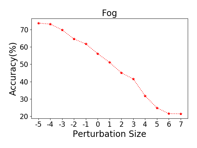
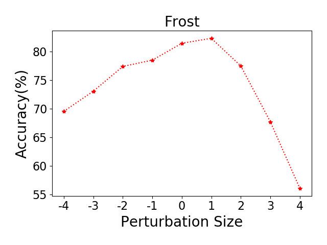
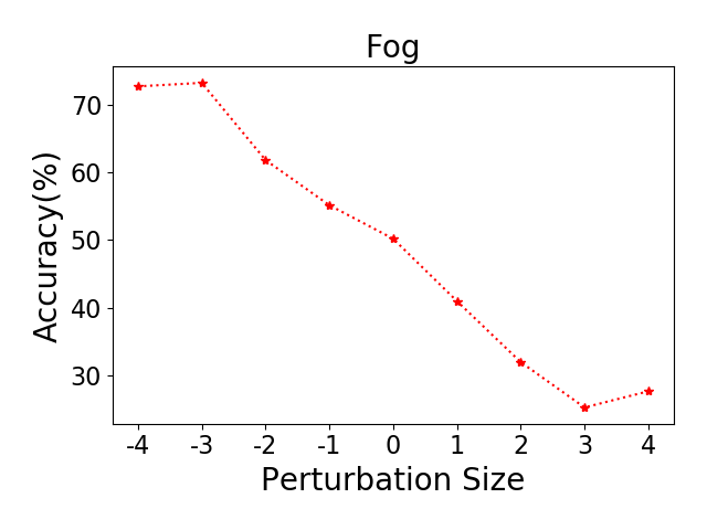
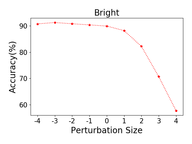
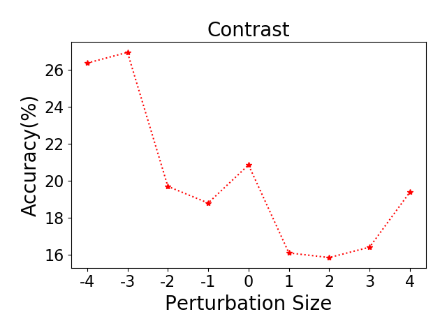
As can be seen, Adv-$\ell_{2}$ and Adv-$\ell_{\infty}$ improve the average accuracy on OOD data, especially under corruption types Noise and Blur. This supports our finding in Section 3 that AT makes the model generalize on OOD data. Though AT improves the OOD generalization on all corruption types for ImageNet-C, it degenerates the performance for data corrupted under types Fog, Bright and Contrast in CIFAR10-C. We speculate this is because these three corruptions intrinsically rescale the adversarial perturbation, and refer readers to Appendix D.1 for a detailed discussion.

Ablation Study.

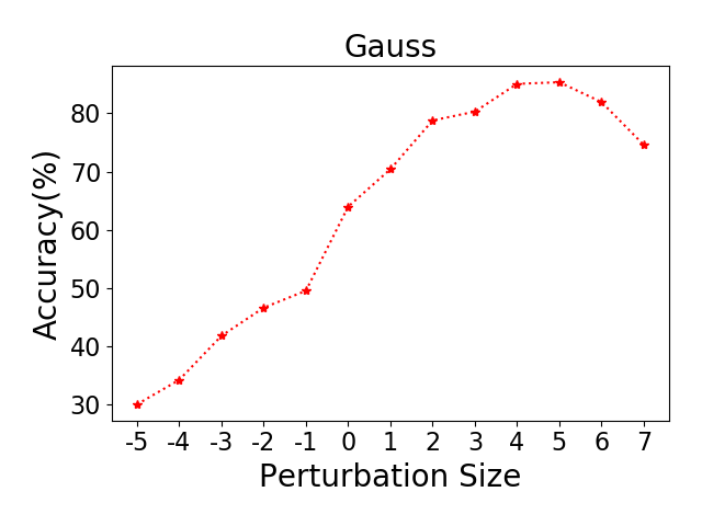
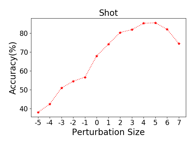
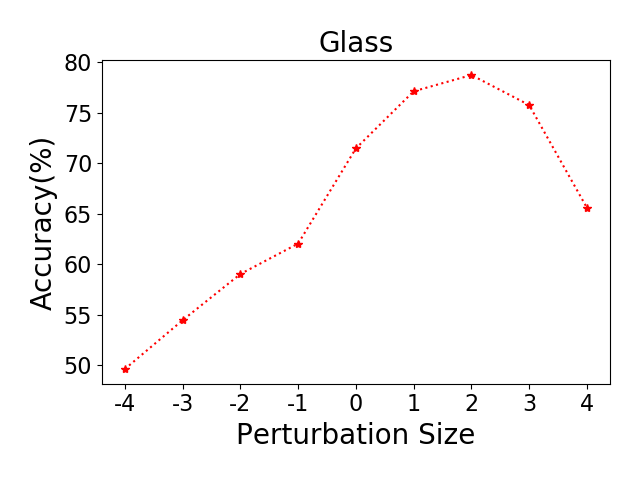
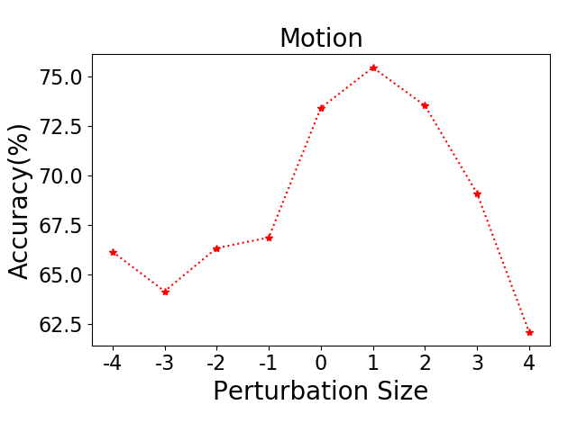
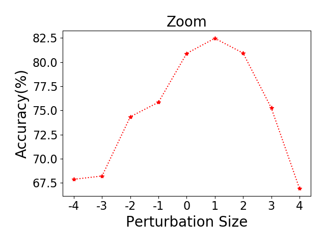
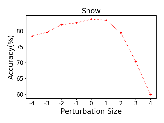
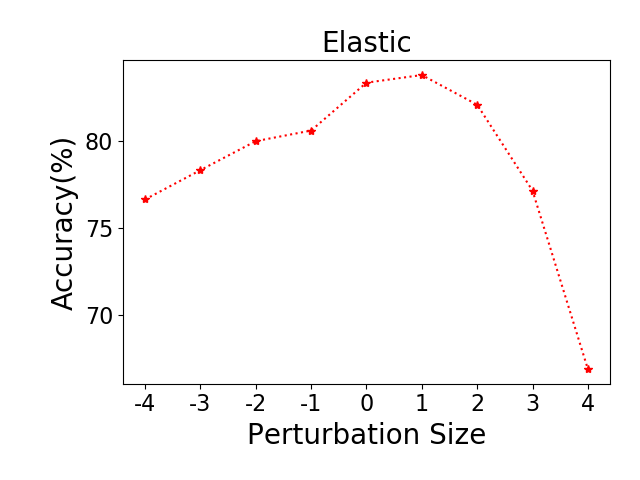
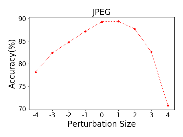
We study the effect of perturbation size $r$ and the number of training samples $n$ for adversarial training in bounds (5) and (6). Due to the space limit, we put the implementation details and results in Appendix D.

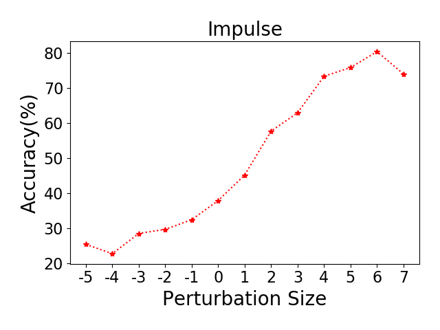
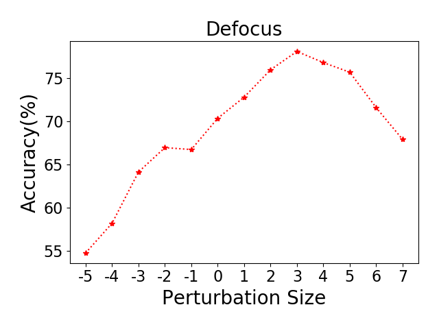
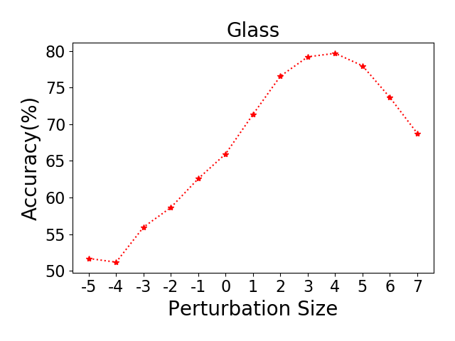
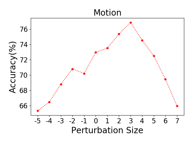
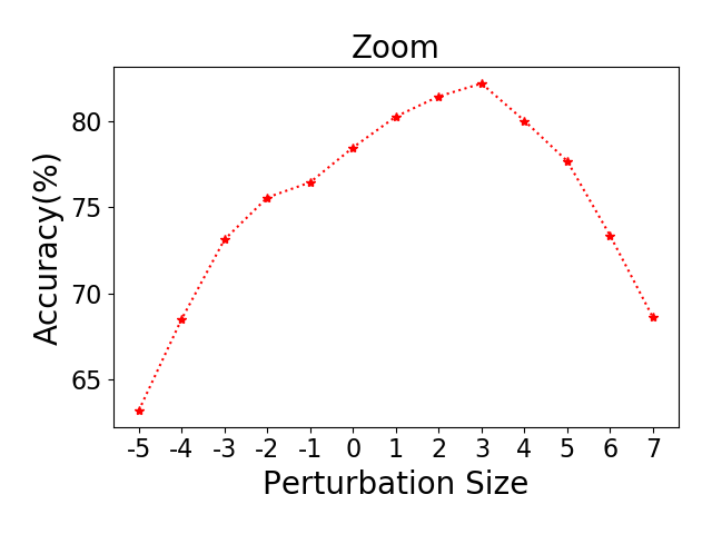
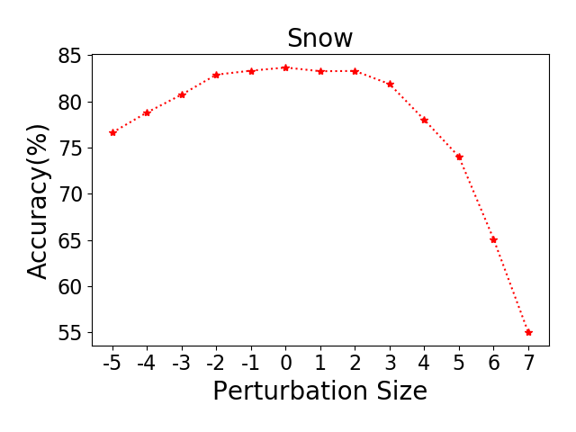
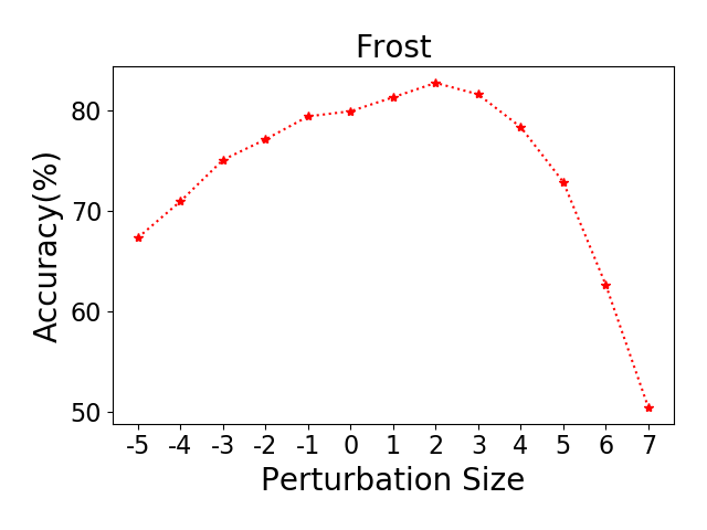
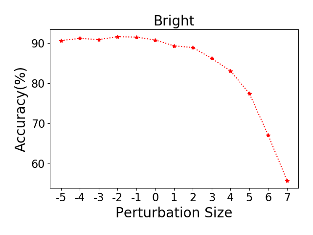
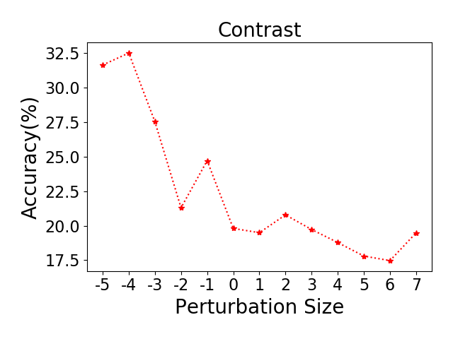
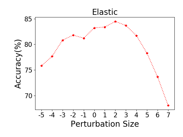
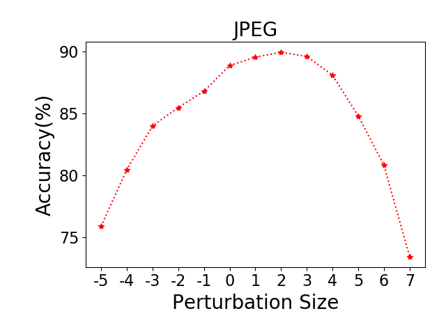
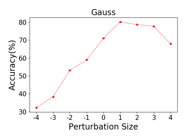
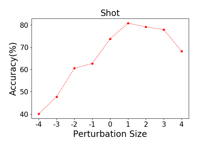
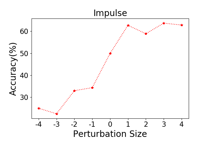
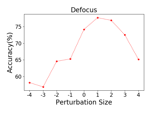
The results for the effect of perturbation size $r$ are in Figures 3-4 in Appendix D.1. As can be seen, the accuracy on OOD data CIFAR10-C first increases and then decreases with an increasing $r$. This is because the upper bounds of excess risk in (5) and (6) are decided by both the clean accuracy and input-robustness. However, an increasing perturbation size $r$ improves the input-robustness, but harms the clean accuracy (Raghunathan et al., 2019). Specifically, when the perturbation size $r$ is small, the clean accuracy is relatively stable and the robustness dominates. Thus the overall OOD performance increases as $r$ increases. However, when $r$ is relatively large, a larger $r$ leads to worse clean accuracy though better robustness, and can lead to worse overall OOD performance. Thus, to achieve the optimal performance on OOD data, we should properly choose the perturbation size $r$ rather than continually increasing it.

The results for the effect of the number of training samples $n$ are in Figures 5-6 in Appendix D.2. The accuracy on OOD data increases with the number of training samples, which is consistent with our findings in Theorems 1 and 2.

5.1.2 Experiments on Natural Language Understanding

Table 2: Performance of BERT base model on NLU tasks using standard training and adversarial training under both $\ell_{2}$-norm and $\ell_{\infty}$-norm.

Dataset	Train	Test	Std	Adv-$\ell_{2}$	Adv-$\ell_{\infty}$
STS-B	Images	Images	98.38	97.81	96.39
		MSRvid	89.52(-8.86)	90.61(-7.20)	90.09(-6.30)
	MSRvid	MSRvid	98.55	97.45	96.65
		Images	84.12(-14.43)	83.63(-13.82)	83.11(-13.54)
	Headlines	Headlines	97.59	96.73	95.75
		MSRpar	62.07(-35.52)	64.48(-32.25)	67.67(-28.08)
	MSRpar	MSRpar	97.55	97.33	97.55
		Headlines	75.58(-21.97)	75.27(-22.06)	76.12(-21.43)
SST-2; IMDb	SST-2	SST-2	93.57	93.57	93.92
		IMDb	90.06(-3.51)	91.50(-2.07)	91.32(-2.60)
	IMDb	IMDb	94.36	94.88	94.68
		SST-2	87.00(-7.36)	88.53(-6.35)	88.07(-6.61)
MNLI	Telephone	Telephone	83.01	83.16	82.90
		Letters	82.45(-0.56)	83.76(+0.60)	84.07(+1.17)
		Face-to-face	81.56(-1.45)	83.59(+0.43)	83.59(+0.69)

Data.

As in (Hendrycks et al., 2020b), we use three pairs of datasets as the original and OOD datasets for NLU tasks.

• SST-2 (Socher et al., 2013) and IMDb (Maas et al., 2011) are sentiment analysis datasets, with pithy expert and full-length lay movie reviews, respectively. As in (Hendrycks et al., 2020b), we train on one dataset and evaluate on the other. Then we report the accuracy of a review’s binary sentiment predicted by the model.

• STS-B consists of texts from different genres and sources. It requires the model to predict the textual similarity between pairs of sentences (Cer et al., 2017). As in (Hendrycks et al., 2020b), we use four sources from two genres: MSRpar(news), Headlines (news); MSRvid(captions), Images(captions). The evaluation metric is Pearson’s correlation coefficient.

• MNLI is a textual entailment dataset which contains sentence pairs from different genres of text (Williams et al., 2018). We select training samples from two genres of transcribed text (Telephone and Face-to-Face) and the other of written text (Letters) as in (Hendrycks et al., 2020b), and report the classification accuracy.

Setup.

For a pre-trained language model e.g., BERT, each input token is encoded as a one-hot vector and then mapped into a continuous embedding space. Instead of adding perturbations to the one-hot vectors, we construct adversarial samples in the word embedding space as in (Zhu et al., 2019).

The backbone model is the base version of BERT (Devlin et al., 2019) which has been widely used in the NLP community. We conduct AT in the fine-tuning stage to see its effectiveness on OOD generalization. The models are trained by AdamW (Loshchilov & Hutter, 2018) for 10 epochs. Detailed hyperparameters are in Appendix C. As in Section 5.1.1, we compare Adv-$\ell_{2}$ and Adv-$\ell_{\infty}$ with Std.

Main Results.

In Table 2, we report the results on in-distribution data and OOD data, and the gap between them (in the brackets) as in (Hendrycks et al., 2020b). The gaps in brackets are used to alleviate the interference by the general benefits from AT itself, since it was shown in (Zhu et al., 2019) that AT can improve the generalization ability of model on in-distribution textual data.

As can be seen, adversarially trained models perform similarly or even better than standardly trained models on in-distribution data, while significantly better on OOD data especially for MNLI. The smaller gaps between in-distribution and OOD data support our finding that AT can be used to improve OOD generalization.

5.2 Robust Pre-Trained Model Improves OOD Generalization

Previously in Section 4, we theoretically show that an input-robust pre-trained model gives a better initialization for fine-tuning on downstream task, in terms of OOD generalization. In this section, we empirically show that this better initialization also leads to better OOD generalization after finetuning on image classification tasks.

Table 3: Clean and corruption accuracy (%) of ResNet34 on CIFAR10-C with no pre-training, standard pre-training, and adversarial pre-training under $\ell_{2}$-norm and $\ell_{\infty}$-norm.

Fine-Tuning	Pre-Training	Clean	Noise			Blur				Weather				Digital				Avg.
			Gauss	Shot	Impulse	Defocus	Glass	Motion	Zoom	Snow	Frost	Fog	Bright	Contrast	Elastic	Pixel	JPEG
Std	No	95.21	40.55	40.64	19.91	83.21	67.77	77.86	90.31	80.71	77.91	67.27	90.88	48.14	80.80	81.99	80.84	68.59
	Std	94.65	41.25	42.91	22.58	85.19	71.03	78.49	90.82	82.78	80.04	67.66	89.97	45.70	83.89	82.03	80.99	69.69
	Adv-$\ell_{2}$	95.06	45.10	50.58	27.57	87.27	72.95	79.08	90.57	83.29	77.25	65.41	90.15	50.41	82.81	78.01	78.95	70.63
	Adv-$\ell_{\infty}$	94.30	40.94	46.42	29.39	87.60	70.79	81.44	90.69	82.77	79.28	68.84	89.19	45.29	83.59	83.13	80.86	70.68
Adv-$l_{2}$	No	94.43	56.82	60.58	29.34	85.44	71.67	81.80	90.08	83.68	80.37	61.68	89.96	34.76	83.76	85.16	83.24	71.89
	Std	94.09	57.64	60.96	26.35	86.78	73.52	82.16	90.46	82.12	80.64	62.58	88.98	34.68	84.29	83.42	83.42	71.87
	Adv-$\ell_{2}$	94.45	58.98	62.99	35.08	87.07	72.29	81.66	91.07	83.53	81.38	62.82	89.52	39.53	84.35	86.60	88.55	73.69
	Adv-$\ell_{\infty}$	95.25	58.64	62.18	29.86	88.15	73.00	82.95	91.98	84.76	83.86	64.76	91.00	37.35	84.65	86.57	88.59	73.89
Adv-$\ell_{\infty}$	No	92.46	80.91	81.69	52.00	79.58	80.94	77.42	80.21	80.57	79.35	35.41	83.15	18.06	83.51	87.79	87.44	72.54
	Std	92.05	80.21	81.06	63.02	77.94	77.80	75.60	80.04	83.77	81.22	41.57	89.94	19.04	82.39	85.49	88.76	73.86
	Adv-$\ell_{2}$	92.55	81.96	82.86	58.95	80.51	82.66	78.21	86.56	81.49	81.10	42.07	89.76	18.56	84.58	88.53	88.05	75.06
	Adv-$\ell_{\infty}$	92.28	81.74	82.37	56.96	80.34	81.90	77.94	85.76	81.48	81.70	42.99	89.00	18.45	84.50	88.07	87.50	74.71

Setup.

Following (Salman et al., 2020a), we pre-train the model on ImageNet and then fine-tune it on CIFAR10. To get an input-robust model in the pre-training stage, we consider adversarially pre-train the model. We compare adversarial pre-training (Adv-$\ell_{2}$ and Adv-$\ell_{\infty}$) against standard pre-training and no pre-training as in Section 5.1.1. In the fine-tuning stage, the data from CIFAR10 are resized to $224\times 224$ as in (Salman et al., 2020a). We also compare stadard fine-tuning and adversarial fine-tuning under both $\ell_{2}$- and $\ell_{\infty}$-norm. After fine-tuning, we verify the OOD generalization on CIFAR10-C. The other settings are the same as Section 5.1.1.

Main Results.

The results are shown in Table 3. As can be seen, for all fine-tuning methods, adversarially pre-trained models consistently achieve better performance on OOD data than standardly pre-trained models or models without pre-training. Thus, the initialization from the adversarially pre-trained input-robust model leads to better OOD generalization on downstream tasks after fine-tuning. In addition, standard pre-training slightly improves the OOD generalization compared with no pre-training when we conduct Adv-$\ell_{\infty}$ fine-tuning or standard fine-tuning. We also observe that for all four kinds of pre-training, adversarial fine-tuning under $\ell_{\infty}$-norm has better performance than $\ell_{2}$-norm. This agrees with the observations in Section 5.1.1. Note that the results of models without pre-training are different from those in Table 1 due to the resized input data.

5.3 Discussion

It is shown in (Hendrycks et al., 2020b) that the language model BERT (Devlin et al., 2019) pre-trained on large corpus generalizes well on downstream OOD data, and RoBERTa (Liu et al., 2019) pre-trained with more training data and updates generalizes even better than BERT. We speculate this is because (i) sufficient pre-training obtains an input-robust model as discussed in Section 4, and this better-initialization leads to better OOD generalization after finetuning as observed in Section 5.2; and (ii) the objective of masked language modeling predicts the masked (perturbed) input tokens and enables a certain amount of input-robustness.

In this section, we empirically show that the model initialized by BERT has higher input-robustness than a randomly initialized model. Besides, compared with BERT, RoBERTa is pre-trained with more training samples and updating steps and the model initialized by it is more robust to input perturbations.

Setup.

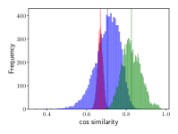
We compare the input-robustness of the base versions of pre-trained language model BERT (Devlin et al., 2019) and RoBERTa (Liu et al., 2019), against a randomly initialized model whose parameters are independently sampled from $\mathcal{N}(0,0.02^{2})$ (Wolf et al., 2020). The three models have exactly the same structure. Compared with BERT, RoBERTa is pre-trained on a larger corpus for more updating steps. Experiments are performed on MRPC and CoLA datasets from the GLUE benchmark (Wang et al., 2018), with 3.7k and 8.5k training samples, respectively. Similar as Section 5.1.2, we add adversarial perturbations in the embedding space. We use 3 steps of $\ell_{\infty}$-norm attack to construct perturbation. The perturbation size is 0.001 and the perturbation step size 0.0005. Since the the last classification layer of BERT or RoBERTa is randomly initialized during downstream task fine-tuning, we study the difference in the hidden states of the last Transformer layer before the classification layer. Denote $\textbf{h},\textbf{h}_{\text{per}}\in\mathbb{R}^{128\times 768}$ as the hidden states from the original input and the adversarially perturbed input, respectively. We use the $\ell_{2}$-norm $\|\textbf{h}_{\text{per}}-\textbf{h}\|$ and the cosine similarity $\langle\textbf{h},\textbf{h}_{\text{per}}\rangle/(\|\textbf{h}\|\|\textbf{h}_{\text{per}}\|)$ to measure the difference. The cosine similarity is used to alleviate the potential interference caused by the scale of h over different pre-trained models. The results are in Figure 1.

(a)

(a) MRPC.

(b) CoLA.

(c) MRPC.

(d) CoLA.

Figure 1: Difference of hidden states in the last Transformer layer between the original input and adversarially perturbed input, measured by $\ell_{2}$-norm and cosine similarity. The models compared are randomly initialized model, BERT, and RoBERTa. The datasets used are MRPC and CoLA from the GLUE benchamrk. The dashed lines in the upper and bottom figures are respectively the mean of $\|\textbf{h}_{\text{per}}-\textbf{h}\|$ and $\langle\textbf{h},\textbf{h}_{\text{per}}\rangle/(\|\textbf{h}\|\|\textbf{h}_{\text{per}}\|)$ from all samples in a dataset.

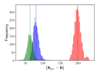
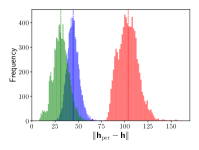
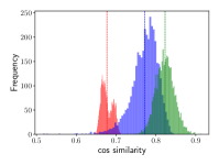
Main Results.

The histograms of $\|\textbf{h}_{\text{per}}-\textbf{h}\|$ and $\langle\textbf{h},\textbf{h}_{\text{per}}\rangle/(\|\textbf{h}\|\|\textbf{h}_{\text{per}}\|)$ from all training samples in MRPC and CoLA are shown in Figure 1a, 1b and Figure 1c, 1d, respectively. We can observe that (i) BERT is more robust than the randomly initialized model, indicating that the masked language modeling objective and sufficient pre-training improves input-robustness, and leads to better ood performance after fine-tuning; (ii) RoBERTa is more input-robust compared with BERT, which implies that that more training samples and updating steps in the pre-training stage improve the input-robustness. Combining with that a more input-robust pre-trained model also leads to better OOD generalization on downstream tasks empirically (Section 4), the above observations (i) and (ii) may also explain the finding in (Hendrycks et al., 2020b) that BERT generalizes worse on downstream OOD data than RoBERTa, but much better than the model without pretraining.

6 Conclusion

In this paper, we explore the relationship between the robustness and OOD generalization of a model. We theoretically show that the input-robust model can generalize well on OOD data under the definition of OOD generalization via Wasserstein distance. Thus, for a model trained from scratch, we suggest using adversarial training to improve the input-robustness of the model which results in better OOD generalization. Under mild conditions, we show that the excess risk on OOD data of an adversarially trained model is upper bounded by $\tilde{\mathcal{O}}(1/\sqrt{n}+1/T)$. For the framework of first pre-training and then fine-tuning, we show that a pre-trained input-robust model provides a theoretically good initialization which empirically improves OOD generalization after fine-tuning. Various experiments on CV and NLP verify our theoretical findings.

Appendix A Proofs for Section 3

A.1 Proofs for Section 3.1

A.1.1 Proof of Theorem 1

To start the proof of Theorem 1, we need the following lemma.

Lemma 1.

For any $w$ and $r$, we have

$$\small\sup_{P\in B_{\mathsf{W}_{\infty}}(P_{0},r)}R_{P}(\text{\boldmath{$w$}})=\mathbb{E}_{P_{0}}\left[\sup_{\|\boldsymbol{\delta}\|_{\infty}\leq r}f(\text{\boldmath{$w$}},\boldsymbol{x}+\boldsymbol{\delta})\right].$$ (16)

Proof.

Let $T_{r}^{\text{\boldmath{$w$}}}(\boldsymbol{x})=\boldsymbol{x}+\arg\max_{\{\boldsymbol{\delta}:\|\boldsymbol{\delta}\|_{\infty}\leq r\}}f(\text{\boldmath{$w$}},\boldsymbol{x}+\boldsymbol{\delta})$ with $\boldsymbol{x}$ is an input data. The existence of $T_{r}^{\text{\boldmath{$w$}}}(\boldsymbol{x})$ is guaranteed by the continuity of $f(\text{\boldmath{$w$}},\boldsymbol{x})$. $P_{r}$ is the distribution of $T_{r}^{\text{\boldmath{$w$}}}(\boldsymbol{x})$ with $\boldsymbol{x}\sim P_{0}$. Then

$$\small\mathbb{E}_{P_{0}}\left[\sup_{\|\boldsymbol{\delta}\|_{\infty}\leq r}f(\text{\boldmath{$w$}},\boldsymbol{x}+\boldsymbol{\delta})\right]=\mathbb{E}_{P_{r}}[f(\text{\boldmath{$w$}},\boldsymbol{x})].$$ (17)

Since

$$\small\mathsf{W}_{\infty}(P_{0},P_{r})\leq\mathbb{E}_{P_{0}}[\|\boldsymbol{x}-T_{r}^{\text{\boldmath{$w$}}}(\boldsymbol{x})\|_{\infty}]\leq r,$$ (18)

we have

$$\small\mathbb{E}_{P_{0}}\left[\sup_{\|\boldsymbol{\delta}\|_{\infty}\leq r}f(\text{\boldmath{$w$}},\boldsymbol{x}+\boldsymbol{\delta})\right]\leq\sup_{P\in B_{\mathsf{W}_{\infty}}(P_{0},r)}R_{P}(\text{\boldmath{$w$}}).$$ (19)

On the other hand, let $P^{*}_{r}\in\arg\max_{P\in B_{\mathsf{W}_{\infty}}(P_{0},r)}R_{P}(\text{\boldmath{$w$}})$. Due to Kolmogorov’s theorem, $P^{*}_{r}$ can be distribution of some random vector $\boldsymbol{z}$, due to the definition of $\mathsf{W}_{\infty}$-distance, we have $\|\boldsymbol{z}-\boldsymbol{x}\|_{\infty}\leq r$ holds almost surely. Then we conclude

$$\small\sup_{P\in B_{\mathsf{W}_{\infty}}(P_{0},r)}R_{P}(\text{\boldmath{$w$}})=R_{P^{*}_{r}}(\text{\boldmath{$w$}})=\mathbb{E}_{P^{*}_{r}}[f(\text{\boldmath{$w$}},\boldsymbol{z})]\leq\mathbb{E}_{P_{0}}\left[\sup_{\|\boldsymbol{\delta}\|_{\infty}\leq r}f(\text{\boldmath{$w$}},\boldsymbol{x}+\boldsymbol{\delta})\right].$$ (20)

Thus, we get the conclusion. ∎

This lemma shows that the distributional perturbation measured by $\mathsf{W}_{\infty}$-distance is equivalent to input perturbation. Hence we can study $\mathsf{W}_{\inf}$-distributional robustness through $\ell_{\inf}$-input-robustness. The basic tool for our proof is the covering number, which is defined as follows.

Definition 2.

(Wainwright, 2019) A $r$-cover of $(\mathcal{X},\|\cdot\|_{p})$ is any point set $\{\boldsymbol{u}_{i}\}\subseteq\mathcal{X}$ such that for any $\boldsymbol{u}\in\mathcal{X}$, there exists $\boldsymbol{u}_{i}$ satisfies $\|\boldsymbol{u}-\boldsymbol{u}_{i}\|_{p}\leq r$. The covering number $\mathcal{N}(r,\mathcal{X},\|\cdot\|_{p})$ is the cardinality of the smallest $r$-cover.

Now we are ready to give the proof of Theorem 1 which is motivated by (Xu & Mannor, 2012).

Proof of Theorem 1.

We can construct a $r$-cover to $(\mathcal{X},\|\cdot\|_{2})$ then $\mathcal{N}(r,\mathcal{X},\|\cdot\|_{2})\leq(2d_{0})^{(2D/r^{2}+1)}=N$, because the $\mathcal{X}$ can be covered by a polytope with $\ell_{2}$-diameter smaller than $2D$ and $2d_{0}$ vertices, see (Vershynin, 2018) Theorem 0.0.4 for details. Due to the geometrical structure, we have $\mathcal{N}(r,\mathcal{X},\|\cdot\|_{\infty})\leq(2d_{0})^{(2D/r^{2}+1)}$. Then, there exists $(C_{1},\cdots,C_{N})$ covers $(\mathcal{X},\|\cdot\|_{\infty})$ where $C_{i}$ is disjoint with each other, and $\|\boldsymbol{u}-\boldsymbol{v}\|_{\infty}\leq r$ for any $\boldsymbol{u},\boldsymbol{v}\in C_{i}$. This can be constructed by $C_{i}=\hat{C}_{i}\bigcap\left(\bigcup_{j=1}^{i-1}\hat{C}_{j}\right)^{c}$ with $(\hat{C}_{1},\cdots,\hat{C}_{N})$ covers $(\mathcal{X},\|\cdot\|_{\infty})$, and the diameter of each $\hat{C}_{i}$ is smaller than $r$ since $\mathcal{N}(r,\mathcal{X},\|\cdot\|_{\infty})\leq N$. Let $A_{j}=\{\boldsymbol{x}_{i}:\boldsymbol{x}_{i}\in C_{j}\}$, and $|A_{j}|$ is the cardinality of $A_{j}$. Due to Lemma 1, we have

$$\left|\sup_{P\in B_{\mathsf{W}_{\infty}}(P_{0},r_{0})}R_{P}(\text{\boldmath{$w$}})-R_{P_{n}}(\text{\boldmath{$w$}})\right| =\left|\mathbb{E}_{P_{0}}\left[\sup_{\|\boldsymbol{\delta}\|_{\infty}\leq r_{0}}f(\text{\boldmath{$w$}},\boldsymbol{x}+\boldsymbol{\delta})\right]-R_{P_{n}}(\text{\boldmath{$w$}})\right|$$ (21)

$$=\left|\sum\limits_{j=1}^{N}\mathbb{E}_{P_{0}}\left[\sup_{\|\boldsymbol{\delta}\|_{\infty}\leq r_{0}}f(\text{\boldmath{$w$}},\boldsymbol{x}+\boldsymbol{\delta})\mid\boldsymbol{x}\in C_{j}\right]P_{0}(C_{j})-R_{P_{n}}(\text{\boldmath{$w$}})\right|$$

$$\leq\left|\sum\limits_{j=1}^{N}\mathbb{E}_{P_{0}}\left[\sup_{\|\boldsymbol{\delta}\|_{\infty}\leq r_{0}}f(\text{\boldmath{$w$}},\boldsymbol{x}+\boldsymbol{\delta})\mid\boldsymbol{x}\in C_{j}\right]\frac{|A_{j}|}{n}-\frac{1}{n}\sum\limits_{i=1}^{n}f(\text{\boldmath{$w$}},\boldsymbol{x}_{i})\right|$$

$$+\left|\sum\limits_{j=1}^{N}\mathbb{E}_{P_{0}}\left[\sup_{\|\boldsymbol{\delta}\|_{\infty}\leq r_{0}}f(\text{\boldmath{$w$}},\boldsymbol{x}+\boldsymbol{\delta})\mid\boldsymbol{x}\in C_{j}\right]\left(\frac{|A_{j}|}{n}-P_{0}(C_{j})\right)\right|$$

$$\leq\left|\frac{1}{n}\sum\limits_{j=1}^{N}\sum\limits_{\boldsymbol{x}_{i}\in C_{j}}\sup_{\boldsymbol{x}\in C_{j}+B_{\infty}(\textbf{0},r_{0})}|f(\text{\boldmath{$w$}},\boldsymbol{x})-f(\text{\boldmath{$w$}},\boldsymbol{x}_{i})|\right|+M\sum\limits_{j=1}^{N}\left|\frac{|A_{j}|}{n}-P_{0}(C_{j})\right|$$

$$\overset{a}{\leq}\frac{1}{n}\sum\limits_{i=1}^{n}\sup_{\|\boldsymbol{\delta}\|_{\infty}\leq 2r}\left|f(\text{\boldmath{$w$}},\boldsymbol{x}_{i}+\boldsymbol{\delta})-f(\text{\boldmath{$w$}},\boldsymbol{x}_{i})\right|+M\sum\limits_{j=1}^{N}\left|\frac{|A_{j}|}{n}-P_{0}(C_{j})\right|$$

$$\leq\epsilon+M\sum\limits_{j=1}^{N}\left|\frac{|A_{j}|}{n}-P_{0}(C_{j})\right|.$$

Here $a$ is due to $C_{j}+B_{\infty}(\textbf{0},r)\subseteq B_{\infty}(\boldsymbol{x}_{i},2r)$ when $\boldsymbol{x}_{i}\in C_{j}$, since $\ell_{\infty}$-diameter of $C_{j}$ is smaller than $r$. The last inequality is due to $(2r,\epsilon,P_{n},\infty)$-robustness of $f(\text{\boldmath{$w$}},\boldsymbol{x})$. On the other hand, due to Proposition A6.6 in (van der Vaart & Wellner, 2000), we have

$$\small\mathbb{P}\left(\sum\limits_{j=1}^{N}\left|\frac{|A_{j}|}{n}-P_{0}(C_{j})\right|\geq\theta\right)\leq 2^{N}\exp\left(\frac{-n\theta^{2}}{2}\right).$$ (22)

Combine this with (21), due to the value of $N$, we get the conclusion. ∎

A.1.2 Proof of Theorem 2

There is a little difference of proving Theorem 2 compared with Theorem 1. Because the out-distribution $P$ constrained in $B_{\mathsf{W}_{\infty}}(P_{0},r)$ only correspond with OOD data that contained in a $\ell_{\infty}$-ball of in-distribution data almost surely, see Lemma 1 for a rigorous description. Hence, we can utilize $\ell_{\infty}$-robustness of model to derive the OOD generalization under $\mathsf{W}_{\infty}$-distance by Theorem 1. However, in the regime of $\mathsf{W}_{2}$-distance, roughly speaking, the transformed OOD data $T_{r}^{\text{\boldmath{$w$}}}(\boldsymbol{x})$ is contained in a $\ell_{2}$-ball of $\boldsymbol{x}$ in expectation. Thus, Lemma 1 is invalid under $\mathsf{W}_{2}$-distance.

To discuss the OOD generalization under $\mathsf{W}_{2}$-distance, we need to give a delicate characterization to the distribution $P\in B_{\mathsf{W}_{2}}(P_{0},r)$. First, we need the following lemma.

Lemma 2.

For any $r$ and $w$, let $P^{*}_{r}\in\arg\max_{P\in B_{\mathsf{W}_{2}}(P_{0},r)}R_{P}(\text{\boldmath{$w$}})$. Then, there exists a mapping $T_{r}^{\text{\boldmath{$w$}}}(\boldsymbol{x})$ such that $T_{r}^{\text{\boldmath{$w$}}}(\boldsymbol{x})\sim P^{*}_{r}$ with $\boldsymbol{x}\sim P_{0}$.

Proof.

The proof of Theorem 6 in (Sinha et al., 2018) shows that

$$\small R_{P^{*}_{r}}(\text{\boldmath{$w$}})=\sup_{P\in B_{\mathsf{W}_{2}}(P_{0},r)}R_{P}(\text{\boldmath{$w$}})=\inf_{\lambda\geq 0}\sup_{P,\pi\in(P,P_{0})}\left(\int_{\mathcal{X}\times\mathcal{X}}f(\text{\boldmath{$w$}},\boldsymbol{x})-\lambda\|\boldsymbol{x}-\boldsymbol{z}\|^{2}d\pi(\boldsymbol{x},\boldsymbol{z})+\lambda r\right).$$ (23)

We next show that the supremum over $\pi$ in the last equality is attained by the joint distribution $(T_{r}^{\text{\boldmath{$w$}}}(\boldsymbol{x}),\boldsymbol{x})$, which implies our conclusion. For any $\lambda>0$, we have

$$\small\sup_{P,\pi\in(P,P_{0})}\left(\int_{\mathcal{X}\times\mathcal{X}}f(\text{\boldmath{$w$}},\boldsymbol{x})-\lambda\|\boldsymbol{x}-\boldsymbol{z}\|^{2}d\pi(\boldsymbol{x},\boldsymbol{z})\right)\leq\int_{\mathcal{X}}\sup_{\boldsymbol{x}}\left(f(\text{\boldmath{$w$}},\boldsymbol{x})-\lambda\|\boldsymbol{x}-\boldsymbol{z}\|^{2}\right)dP_{0}(\boldsymbol{z}),$$ (24)

due to the supremum in the left hand side is taken over $P$ and $\pi$. On the other hand, let $P(\cdot\mid\boldsymbol{z})$ and $\boldsymbol{x}(\cdot)$ respectively be the regular conditional distribution on $\mathcal{X}$ with $\boldsymbol{z}$ given and the function on $\mathcal{X}$. Since $P(\cdot\mid\boldsymbol{z})$ is measurable,

$$\sup_{P,\pi\in(P,P_{0})}\left(\int_{\mathcal{X}\times\mathcal{X}}f(\text{\boldmath{$w$}},\boldsymbol{x})-\lambda\|\boldsymbol{x}-\boldsymbol{z}\|^{2}d\pi(\boldsymbol{x},\boldsymbol{z})\right) \geq\sup_{P(\cdot\mid\boldsymbol{z})}\left(\int_{\mathcal{X}\times\mathcal{X}}f(\text{\boldmath{$w$}},\boldsymbol{x})-\lambda\|\boldsymbol{x}-\boldsymbol{z}\|^{2}dP(\boldsymbol{x}\mid\boldsymbol{z})dP_{0}(\boldsymbol{z})\right)$$ (25)

$$\geq\sup_{\boldsymbol{x}(\cdot)}\left(\int_{\mathcal{X}}f(\text{\boldmath{$w$}},\boldsymbol{x}(\boldsymbol{z}))-\lambda\|\boldsymbol{x}(\boldsymbol{z})-\boldsymbol{z}\|^{2}dP_{0}(\boldsymbol{z})\right)$$

$$\geq\int_{\mathcal{X}}\sup_{\boldsymbol{x}}\left(f(\text{\boldmath{$w$}},\boldsymbol{x})-\lambda\|\boldsymbol{x}-\boldsymbol{z}\|^{2}\right)dP_{0}(\boldsymbol{z}).$$

Thus, we get the conclusion. ∎

Proof of Theorem 2.

Similar to the proof of Theorem 1, we can construct a disjoint cover $(C_{1},\cdots,C_{N})$ to $(\mathcal{X},\|\cdot\|_{2})$ such that $N\leq(2d_{0})^{(2\epsilon^{2}D/r^{2}+1)}$, and the $l_{2}$-diameter of each $C_{i}$ is smaller than $r/\epsilon$. Let $P^{*}_{r}\in\arg\max_{P\in B_{\mathsf{W}_{2}}(P_{0},r)}R_{P}(\text{\boldmath{$w$}})$, by Lemma 2, we have

$$\sup_{P\in B_{\mathsf{W}_{2}}(P_{0},r)}R_{P}(\text{\boldmath{$w$}}) =R_{P^{*}_{r}}(\text{\boldmath{$w$}})$$ (26)

$$=\mathbb{E}_{P_{0}}\left[f(\text{\boldmath{$w$}},T_{r}^{\text{\boldmath{$w$}}}(\boldsymbol{x}))\right]$$

$$=\mathbb{E}_{P_{0}}\left[f(\text{\boldmath{$w$}},T_{r}^{\text{\boldmath{$w$}}}(\boldsymbol{x}))\left(\textbf{1}_{T_{r}^{\text{\boldmath{$w$}}}(\boldsymbol{x})\in B_{2}(\boldsymbol{x},r/\epsilon)}+\textbf{1}_{T_{r}^{\text{\boldmath{$w$}}}(\boldsymbol{x})\notin B_{2}(\boldsymbol{x},r/\epsilon)}\right)\right]$$

$$\leq\mathbb{E}_{P_{0}}\left[\sup_{\|\boldsymbol{\delta}\|_{2}\leq r/\epsilon}f(\text{\boldmath{$w$}},\boldsymbol{x}+\boldsymbol{\delta})\right]+M\mathbb{P}(T_{r}^{\text{\boldmath{$w$}}}(\boldsymbol{x})\notin B_{2}(\boldsymbol{x},r/\epsilon)).$$

Due to the definition of $T_{r}^{\text{\boldmath{$w$}}}(\boldsymbol{x})$, by Markov’s inequality, we have

$$\small\left(\frac{r}{\epsilon}\right)\mathbb{P}(T_{r}^{\text{\boldmath{$w$}}}(\boldsymbol{x})\notin B_{2}(\boldsymbol{x},r/\epsilon))\leq\int_{\mathcal{X}}\|T_{r}^{\text{\boldmath{$w$}}}(\boldsymbol{x})-\boldsymbol{x}\|^{2}dP_{0}(\boldsymbol{x})=\mathsf{W}_{2}(P_{0},P^{*}_{r})\leq r.$$ (27)

Plugging this into (26), and due to the definition of Wasserstein distance, we have

$$\small\mathbb{E}_{P_{0}}\left[\sup_{\|\boldsymbol{\delta}\|_{2}\leq r/\epsilon}f(\text{\boldmath{$w$}},\boldsymbol{x}+\boldsymbol{\delta})\right]\leq\sup_{P\in B_{\mathsf{W}_{2}}(P_{0},r)}R_{P}(\text{\boldmath{$w$}})\leq\mathbb{E}_{P_{0}}\left[\sup_{\|\boldsymbol{\delta}\|_{2}\leq r/\epsilon}f(\text{\boldmath{$w$}},\boldsymbol{x}+\boldsymbol{\delta})\right]+M\epsilon.$$ (28)

Similar to the proof of Theorem 1, due to the model is $(2r/\epsilon,\epsilon,P_{n},2)$-robust, we have

$$\small\left|\mathbb{E}_{P_{0}}\left[\sup_{\|\boldsymbol{\delta}\|_{2}\leq r/\epsilon}f(\text{\boldmath{$w$}},\boldsymbol{x}+\boldsymbol{\delta})\right]-R_{P_{n}}(\text{\boldmath{$w$}})\right|\leq\epsilon+M\sqrt{\frac{(2d_{0})^{(2\epsilon^{2}D/r^{2}+1)}\log{2}+2\log{(1/\theta)}}{n}}$$ (29)

holds with probability at least $1-\theta$. Combining this with (28), we get the conclusion. ∎

A.2 Proofs for Section 3.2

The proof of Theorem 3 is same for $p\in\{2,\infty\}$, we take $p=\infty$ as an example. Before providing the proof, we first give a lemma to characterize the convergence rate of the first inner loop in Algorithm 1.

Lemma 3.

For any $\text{\boldmath{$w$}},\boldsymbol{x}\in\{\boldsymbol{x}_{i}\}$, and $r$, there exists $\boldsymbol{\delta}^{*}\in\arg\max_{\{\boldsymbol{\delta}:\|\boldsymbol{\delta}\|_{\infty}\leq r\}}f(\text{\boldmath{$w$}},\boldsymbol{x}+\boldsymbol{\delta})$ such that

$$\small\|\boldsymbol{\delta}_{K+1}-\boldsymbol{\delta}^{*}\|^{2}\leq\left(1-\frac{\mu_{\boldsymbol{x}}}{L_{22}}\right)^{K}\|\boldsymbol{\delta}_{1}-\boldsymbol{\delta}^{*}\|^{2}$$ (30)

when $\boldsymbol{\delta}_{k+1}=\emph{\text{Proj}}_{B_{\infty}(\emph{{0}},r)}\left(\boldsymbol{\delta}_{k}+\eta_{\boldsymbol{x}}\nabla_{\boldsymbol{x}}f(\text{\boldmath{$w$}},\boldsymbol{x}+\boldsymbol{\delta}_{k})\right)$ with $\eta_{\boldsymbol{x}}=1/L_{22}$.

Proof.

The existence of $\boldsymbol{\delta}^{*}$ is due to the continuity of $f(\text{\boldmath{$w$}},\cdot)$. Then

$$f(\text{\boldmath{$w$}},\boldsymbol{x}+\boldsymbol{\delta}^{*})-f(\text{\boldmath{$w$}},\boldsymbol{x}+\boldsymbol{\delta}_{k+1}) =f(\text{\boldmath{$w$}},\boldsymbol{x}+\boldsymbol{\delta}^{*})-f(\text{\boldmath{$w$}},\boldsymbol{x}+\boldsymbol{\delta}_{k})+f(\text{\boldmath{$w$}},\boldsymbol{x}+\boldsymbol{\delta}_{k})-f(\text{\boldmath{$w$}},\boldsymbol{x}+\boldsymbol{\delta}_{k+1})$$ (31)

$$\overset{a}{\leq}\langle\nabla_{\boldsymbol{x}}f(\text{\boldmath{$w$}},\boldsymbol{x}+\boldsymbol{\delta}_{k}),\boldsymbol{\delta}^{*}-\boldsymbol{\delta}_{k}\rangle-\frac{\mu_{\boldsymbol{x}}}{2}\|\boldsymbol{\delta}_{k}-\boldsymbol{\delta}^{*}\|^{2}$$

$$+\langle\nabla_{\boldsymbol{x}}f(\text{\boldmath{$w$}},\boldsymbol{x}+\boldsymbol{\delta}_{k}),\boldsymbol{\delta}_{k}-\boldsymbol{\delta}_{k+1}\rangle+\frac{L_{22}}{2}\|\boldsymbol{\delta}_{k+1}-\boldsymbol{\delta}_{k}\|^{2}$$

$$=\langle\nabla_{\boldsymbol{x}}f(\text{\boldmath{$w$}},\boldsymbol{x}+\boldsymbol{\delta}_{k}),\boldsymbol{\delta}^{*}-\boldsymbol{\delta}_{k+1}\rangle-\frac{\mu_{\boldsymbol{x}}}{2}\|\boldsymbol{\delta}_{k}-\boldsymbol{\delta}^{*}\|^{2}+\frac{L_{22}}{2}\|\boldsymbol{\delta}_{k+1}-\boldsymbol{\delta}_{k}\|^{2}$$

$$\overset{b}{\leq}L_{22}\langle\boldsymbol{\delta}_{k+1}-\boldsymbol{\delta}_{k},\boldsymbol{\delta}^{*}-\boldsymbol{\delta}_{k+1}\rangle-\frac{\mu_{\boldsymbol{x}}}{2}\|\boldsymbol{\delta}_{k}-\boldsymbol{\delta}^{*}\|^{2}+\frac{L_{22}}{2}\|\boldsymbol{\delta}_{k+1}-\boldsymbol{\delta}_{k}\|^{2}$$

$$=L_{22}\langle\boldsymbol{\delta}_{k+1}-\boldsymbol{\delta}_{k},\boldsymbol{\delta}^{*}-\boldsymbol{\delta}_{k}\rangle-\frac{\mu_{\boldsymbol{x}}}{2}\|\boldsymbol{\delta}_{k}-\boldsymbol{\delta}^{*}\|^{2}-\frac{L_{22}}{2}\|\boldsymbol{\delta}_{k+1}-\boldsymbol{\delta}_{k}\|^{2},$$

where $a$ is due to the $L_{22}$-Lipschitz continuity of $\nabla_{\boldsymbol{x}}f(\text{\boldmath{$w$}},\boldsymbol{x})$ and strongly convexity, $b$ is because the property of projection (see Lemma 3.1 in (Bubeck, 2014)). Then we get

$$\|\boldsymbol{\delta}_{k+1}-\boldsymbol{\delta}^{*}\|^{2} =\|\boldsymbol{\delta}_{k+1}-\boldsymbol{\delta}_{k}\|^{2}+\|\boldsymbol{\delta}_{k}-\boldsymbol{\delta}^{*}\|^{2}+2\langle\boldsymbol{\delta}_{k+1}-\boldsymbol{\delta}_{k},\boldsymbol{\delta}_{k}-\boldsymbol{\delta}^{*}\rangle$$ (32)

$$\leq\left(1-\frac{\mu_{\boldsymbol{x}}}{L_{22}}\right)\|\boldsymbol{\delta}_{k}-\boldsymbol{\delta}^{*}\|^{2}$$

by plugging (31) into the above equality and $f(\text{\boldmath{$w$}},\boldsymbol{x}+\boldsymbol{\delta}^{*})-f(\text{\boldmath{$w$}},\boldsymbol{x}+\boldsymbol{\delta}_{k+1})\geq 0$. Thus, we get the conclusion. ∎

This lemma shows that the inner loop in Algorithm 1 can efficiently approximate the worst-case perturbation for any $\text{\boldmath{$w$}}_{t}$ and $\boldsymbol{x}_{i}$. Now we are ready to give the proof of Theorem 3.

We need the following lemma, which is Theorem 6 in (Rakhlin et al., 2012).

Lemma 4.

Let $\{\xi_{1},\cdots,\xi_{t}\}$ be a martingale difference sequence with a uniform upper bound $b$. Let $V_{t}=\sum_{j=1}^{t}\mathsf{Var}(\xi_{j}\mid\mathcal{F}_{j-1})$ with $\mathcal{F}_{j}$ is the $\sigma$-field generated by $\{\xi_{1},\cdots,\xi_{j}\}$. Then for every $a$ and $v>0$,

$$\small\mathbb{P}\left(\bigcup_{s\leq t}\left(\left\{\sum\limits_{j=1}^{t}\xi_{j}\geq a\right\}\bigcap\left\{V_{t}\leq v\right\}\right)\right)\leq\exp\left(\frac{-a^{2}}{2(v+ba)}\right).$$ (33)

This is a type of Bennett’s inequality which is sharper compared with Azuma-Hoeffding’s inequality when the variance $v$ is much smaller than uniform bound $b$.

A.2.1 Proof of Theorem 3

Proof.

With a little abuse of notation, let $r(p)=r$ and define $g(\text{\boldmath{$w$}},\boldsymbol{x})=\sup_{\boldsymbol{\delta}:\|\boldsymbol{\delta}\|_{\infty}\leq r}f(\text{\boldmath{$w$}},\boldsymbol{x}+\boldsymbol{\delta})$. Lemma A.5 in (Nouiehed et al., 2019) implies $g(\text{\boldmath{$w$}},\boldsymbol{x})$ has $L_{11}+\frac{L_{12}L_{21}}{\mu_{\boldsymbol{x}}}$-Lipschitz continuous gradient with respect to $w$ for any specific $\boldsymbol{x}$. Then $\tilde{R}_{P_{n}}(\text{\boldmath{$w$}})$ has $L=L_{11}+\frac{L_{12}L_{21}}{\mu_{\boldsymbol{x}}}$-Lipschitz continuous gradient. Let $\boldsymbol{x}^{*}\in\boldsymbol{x}+\arg\max_{\{\boldsymbol{\delta}:\|\boldsymbol{\delta}\|_{\infty}\leq r\}}f(\text{\boldmath{$w$}},\boldsymbol{x}+\boldsymbol{\delta})$, due to the Lipschitz gradient of $\tilde{R}_{P_{n}}(\text{\boldmath{$w$}})$,

$$\tilde{R}_{P_{n}}(\text{\boldmath{$w$}}_{t+1})-\tilde{R}_{P_{n}}(\text{\boldmath{$w$}}_{t}) \leq\langle\nabla\tilde{R}_{P_{n}}(\text{\boldmath{$w$}}_{t}),\text{\boldmath{$w$}}_{t+1}-\text{\boldmath{$w$}}_{t}\rangle+\frac{L}{2}\|\text{\boldmath{$w$}}_{t+1}-\text{\boldmath{$w$}}_{t}\|^{2}$$ (34)

$$=-\eta_{\text{\boldmath{$w$}}_{t}}\langle\nabla\tilde{R}_{P_{n}}(\text{\boldmath{$w$}}_{t}),\nabla_{\text{\boldmath{$w$}}}f(\text{\boldmath{$w$}}_{t},\boldsymbol{x}_{i_{t}}+\boldsymbol{\delta}_{K})\rangle+\frac{\eta_{\text{\boldmath{$w$}}_{t}}^{2}L}{2}\|\nabla_{\text{\boldmath{$w$}}}f(\text{\boldmath{$w$}}_{t},\boldsymbol{x}_{i_{t}}+\boldsymbol{\delta}_{K})\|^{2}$$

$$=-\eta_{\text{\boldmath{$w$}}_{t}}\|\nabla\tilde{R}_{P_{n}}(\text{\boldmath{$w$}}_{t})\|^{2}+\eta_{\text{\boldmath{$w$}}_{t}}\langle\nabla\tilde{R}_{P_{n}}(\text{\boldmath{$w$}}_{t}),\nabla_{\text{\boldmath{$w$}}}f(\text{\boldmath{$w$}}_{t},\boldsymbol{x}_{i_{t}}^{*})-\nabla_{\text{\boldmath{$w$}}}f(\text{\boldmath{$w$}}_{t},\boldsymbol{x}_{i_{t}}+\boldsymbol{\delta}_{K})\rangle$$

$$+\eta_{\text{\boldmath{$w$}}_{t}}\langle\nabla\tilde{R}_{P_{n}}(\text{\boldmath{$w$}}_{t}),\nabla\tilde{R}_{P_{n}}(\text{\boldmath{$w$}}_{t})-\nabla_{\text{\boldmath{$w$}}}f(\text{\boldmath{$w$}}_{t},\boldsymbol{x}_{i_{t}}^{*})\rangle+\frac{\eta_{\text{\boldmath{$w$}}_{t}}^{2}L}{2}\|\nabla_{\text{\boldmath{$w$}}}f(\text{\boldmath{$w$}}_{t},\boldsymbol{x}_{i_{t}}+\boldsymbol{\delta}_{K})\|^{2}.$$

Here the last equality is due to $\nabla_{\text{\boldmath{$w$}}}g(\text{\boldmath{$w$}},\boldsymbol{x})=\nabla_{\text{\boldmath{$w$}}}f(\text{\boldmath{$w$}},\boldsymbol{x}^{*})$ (Similar to Danskin’s theorem, see Lemma A.5 in (Nouiehed et al., 2019)), and $\boldsymbol{x}^{*}_{i_{t}}$ is the local maxima approximated by $\boldsymbol{x}_{i_{t}}+\boldsymbol{\delta}_{K}$ in Lemma 3. By taking expectation to $\text{\boldmath{$w$}}_{t+1}$ with $\text{\boldmath{$w$}}_{t}$ given in the both side of the above equation, Jesen’s inequality, combining Lemma 3 and $\eta_{\text{\boldmath{$w$}}_{t}}=1/\mu_{\text{\boldmath{$w$}}}t$,

$$\mathbb{E}[\tilde{R}_{P_{n}}(\text{\boldmath{$w$}}_{t+1})]-\tilde{R}_{P_{n}}(\text{\boldmath{$w$}}^{*}) \leq\tilde{R}_{P_{n}}(\text{\boldmath{$w$}}_{t})-\tilde{R}_{P_{n}}(\text{\boldmath{$w$}}^{*})-\eta_{\text{\boldmath{$w$}}_{t}}\|\nabla\tilde{R}_{P_{n}}(\text{\boldmath{$w$}}_{t})\|^{2}$$ (35)

$$+\mathbb{E}\left[\eta_{\text{\boldmath{$w$}}_{t}}\|\nabla\tilde{R}_{P_{n}}(\text{\boldmath{$w$}}_{t})\|\|\nabla_{\text{\boldmath{$w$}}}f(\text{\boldmath{$w$}}_{t},\boldsymbol{x}_{i_{t}}^{*})-\nabla_{\text{\boldmath{$w$}}}f(\text{\boldmath{$w$}},\boldsymbol{x}_{i_{t}}+\boldsymbol{\delta}_{K})\|\right]+\frac{\eta_{\text{\boldmath{$w$}}_{t}}^{2}G^{2}L}{2}$$

$$\leq\tilde{R}_{P_{n}}(\text{\boldmath{$w$}}_{t})-\tilde{R}_{P_{n}}(\text{\boldmath{$w$}}^{*})-\eta_{\text{\boldmath{$w$}}_{t}}\|\nabla\tilde{R}_{P_{n}}(\text{\boldmath{$w$}}_{t})\|^{2}+\eta_{\text{\boldmath{$w$}}_{t}}\|\nabla\tilde{R}_{P_{n}}(\text{\boldmath{$w$}}_{t})\|\left(1-\frac{\mu_{\boldsymbol{x}}}{L_{22}}\right)^{K}\mathbb{E}\left[\|\boldsymbol{\delta}_{1}-\boldsymbol{\delta}_{i_{t}}^{*}\|^{2}\right]+\frac{\eta_{\text{\boldmath{$w$}}_{t}}^{2}G^{2}L}{2}$$

$$\leq\left(1-2\mu_{\text{\boldmath{$w$}}}\eta_{\text{\boldmath{$w$}}_{t}}\right)\left(\tilde{R}_{P_{n}}(\text{\boldmath{$w$}}_{t})-\tilde{R}_{P_{n}}(\text{\boldmath{$w$}}^{*})\right)+\eta_{\text{\boldmath{$w$}}_{t}}^{2}G^{2}L$$

$$=\left(1-\frac{2}{t}\right)\left(\tilde{R}_{P_{n}}(\text{\boldmath{$w$}}_{t})-\tilde{R}_{P_{n}}(\text{\boldmath{$w$}}^{*})\right)+\frac{G^{2}L}{\mu_{\text{\boldmath{$w$}}}^{2}t^{2}}.$$

Here the third inequality is because

$$\small\eta_{\text{\boldmath{$w$}}_{t}}\|\nabla\tilde{R}_{P_{n}}(\text{\boldmath{$w$}}_{t})\|\left(1-\frac{\mu_{\boldsymbol{x}}}{L_{22}}\right)^{K}\|\boldsymbol{\delta}_{1}-\boldsymbol{\delta}_{i_{t}}^{*}\|^{2}\leq\eta_{\text{\boldmath{$w$}}_{t}}G\left(1-\frac{\mu_{\boldsymbol{x}}}{L_{22}}\right)^{K}4d_{0}r^{2}\leq\frac{\eta_{\text{\boldmath{$w$}}_{t}}^{2}G^{2}L}{2},$$ (36)

for any $\boldsymbol{\delta}_{i_{t}}^{*}$, since

$$\small K\log{\left(1-\frac{\mu_{\boldsymbol{x}}}{L_{22}}\right)}\leq-K\frac{\mu_{\boldsymbol{x}}}{L_{22}}\leq\log{\left(\frac{GL}{8T\mu_{\text{\boldmath{$w$}}}d_{0}r^{2}}\right)}.$$ (37)

Then by induction,

$$\mathbb{E}[\tilde{R}_{P_{n}}(\text{\boldmath{$w$}}_{t+1})]-\tilde{R}_{P_{n}}(\text{\boldmath{$w$}}^{*}) \leq\frac{G^{2}L}{\mu^{2}_{\text{\boldmath{$w$}}}}\sum\limits_{j=2}^{t}\frac{1}{j^{2}}\prod_{k=j+1}^{t}\left(1-\frac{2}{k}\right)$$ (38)

$$=\frac{G^{2}L}{\mu^{2}_{\text{\boldmath{$w$}}}}\sum\limits_{j=2}^{t}\frac{1}{j^{2}}\frac{(j-1)j}{(t-1)t}$$

$$\leq\frac{G^{2}L}{t\mu^{2}_{\text{\boldmath{$w$}}}}.$$

Thus we get the first conclusion of convergence in expectation by taking $t=T$ for $t\geq 2$. For the second conclusion, let us define $\xi_{t}=\langle\nabla\tilde{R}_{P_{n}}(\text{\boldmath{$w$}}_{t}),\nabla\tilde{R}_{P_{n}}(\text{\boldmath{$w$}}_{t})-\nabla_{\text{\boldmath{$w$}}}f(\text{\boldmath{$w$}}_{t},\boldsymbol{x}_{i_{t}}^{*})\rangle$. Then Schwarz inequality implies that

$$\small|\xi_{t}|\leq\|\nabla\tilde{R}_{P_{n}}(\text{\boldmath{$w$}}_{t})\|\|\nabla\tilde{R}_{P_{n}}(\text{\boldmath{$w$}}_{t})-\nabla_{\text{\boldmath{$w$}}}f(\text{\boldmath{$w$}}_{t},\boldsymbol{x}_{i_{t}}^{*})\|\leq 2G^{2}.$$ (39)

Similar to (35), for $t\geq 2$,

$$\tilde{R}_{P_{n}}(\text{\boldmath{$w$}}_{t+1})-\tilde{R}_{P_{n}}(\text{\boldmath{$w$}}^{*}) \leq\left(1-2\mu_{\text{\boldmath{$w$}}}\eta_{\text{\boldmath{$w$}}_{t}}\right)\left(\tilde{R}_{P_{n}}(\text{\boldmath{$w$}}_{t})-\tilde{R}_{P_{n}}(\text{\boldmath{$w$}}^{*})\right)+\eta_{\text{\boldmath{$w$}}_{t}}^{2}G^{2}L+2\eta_{\text{\boldmath{$w$}}_{t}}\xi_{t}$$ (40)

$$\leq\frac{G^{2}L}{t\mu^{2}_{\text{\boldmath{$w$}}}}+\frac{2}{\mu_{\text{\boldmath{$w$}}}}\sum\limits_{j=2}^{t}\frac{\xi_{j}}{j}\prod_{k=j+1}^{t}\left(1-\frac{2}{k}\right)$$

$$=\frac{G^{2}L}{t\mu^{2}_{\text{\boldmath{$w$}}}}+\frac{2}{\mu_{\text{\boldmath{$w$}}}}\sum\limits_{j=2}^{t}\frac{1}{j}\frac{(j-1)j}{(t-1)t}\xi_{j}$$

$$=\frac{G^{2}L}{t\mu^{2}_{\text{\boldmath{$w$}}}}+\frac{2}{\mu_{\text{\boldmath{$w$}}}}\sum\limits_{j=2}^{t}\frac{(j-1)}{(t-1)t}\xi_{j}.$$

Since the second term in the last inequality is upper bonded by $\sum_{j=2}^{t}\xi_{j}$ which is a sum of martingale difference, and $|\xi_{j}|\leq 2G^{2}$, a simple Azuma-Hoeffding’s inequality based on bounded martingale difference (Corollary 2.20 in (Wainwright, 2019)) can give a $\mathcal{O}(1/\sqrt{t})$ convergence rate in the high probability. However, we can sharpen the convergence rate via a Bennett’s inequality (Proposition 3.19 in (Duchi, 2016)), because the conditional variance of $\xi_{j}$ will decrease across training. We consider the conditional variance of $\sum_{j=2}^{t}(j-1)\xi_{j}$, let $\mathcal{F}_{j}$ be the $\sigma$-field generated by $\{\text{\boldmath{$w$}}_{1},\cdots,\text{\boldmath{$w$}}_{j}\}$, since $\mathbb{E}[\xi_{j}]=0$ we have

$$\mathsf{Var}\left(\sum_{j=2}^{t}(j-1)\xi_{j}\mid\mathcal{F}_{j-1}\right) =\sum_{j=2}^{t}(j-1)^{2}\mathsf{Var}\left(\xi_{j}\mid\mathcal{F}_{j-1}\right)$$ (41)

$$=\sum_{j=2}^{t}(j-1)^{2}\mathbb{E}\left[\xi_{j}^{2}\mid\mathcal{F}_{j-1}\right]$$

$$\leq 4G^{2}\sum_{j=2}^{t}(j-1)^{2}\|\nabla\tilde{R}_{P_{n}}(\text{\boldmath{$w$}}_{j})\|^{2}$$

$$\leq 8G^{2}L\sum_{j=2}^{t}(j-1)^{2}\left(\tilde{R}_{P_{n}}(\text{\boldmath{$w$}}_{j})-\tilde{R}_{P_{n}}(\text{\boldmath{$w$}}^{*})\right),$$

where first inequality is from Schwarz’s inequality and the last inequality is because

$$\tilde{R}_{P_{n}}\left(\text{\boldmath{$w$}}^{*}\right)-\tilde{R}_{P_{n}}(\text{\boldmath{$w$}}) \leq\tilde{R}_{P_{n}}\left(\text{\boldmath{$w$}}-\frac{1}{L}\nabla\tilde{R}_{P_{n}}(\text{\boldmath{$w$}})\right)-\tilde{R}_{P_{n}}(\text{\boldmath{$w$}})$$ (42)

$$\leq-\left\langle\nabla\tilde{R}_{P_{n}}(\text{\boldmath{$w$}}),\frac{1}{L}\nabla\tilde{R}_{P_{n}}(\text{\boldmath{$w$}})\right\rangle+\frac{L}{2}\left\|\frac{1}{L}\nabla\tilde{R}_{P_{n}}(\text{\boldmath{$w$}})\right\|^{2}$$

$$=-\frac{1}{2L}\left\|\nabla\tilde{R}_{P_{n}}(\text{\boldmath{$w$}})\right\|^{2},$$

for any $w$. By applying Lemma 4, as long as $T\geq 4$ and $0<\theta<1/e$, then with probability at least $1-\theta$, for all $t\leq T$,

$$\tilde{R}_{P_{n}}(\text{\boldmath{$w$}}_{t+1})-\tilde{R}_{P_{n}}(\text{\boldmath{$w$}}^{*})$$ (43)

$$\leq\frac{8G}{\mu_{\text{\boldmath{$w$}}}(t-1)t}\max\left\{\sqrt{2L\sum_{j=2}^{t}(j-1)^{2}\left(\tilde{R}_{P_{n}}(\text{\boldmath{$w$}}_{j})-\tilde{R}_{P_{n}}(\text{\boldmath{$w$}}^{*})\right)},G(t-1)\sqrt{\log{\left(\frac{\log{T}}{\theta}\right)}}\right\}\sqrt{\log{\left(\frac{\log{T}}{\theta}\right)}}+\frac{G^{2}L}{t\mu^{2}_{\text{\boldmath{$w$}}}}$$

$$\leq\frac{8G\sqrt{\log{(\log{(T/\theta)})}}}{\mu_{\text{\boldmath{$w$}}}(t-1)t}\sqrt{2L\sum_{j=2}^{t}(j-1)^{2}\left(\tilde{R}_{P_{n}}(\text{\boldmath{$w$}}_{j})-\tilde{R}_{P_{n}}(\text{\boldmath{$w$}}^{*})\right)}+\frac{(8\mu_{\text{\boldmath{$w$}}}G^{2}\log{(\log{(T/\theta)})}+G^{2}L)}{t\mu_{\text{\boldmath{$w$}}}^{2}}.$$

Then, an upper bound to the first term in the last inequality can give our conclusion. Note that if $\tilde{R}_{P_{n}}(\text{\boldmath{$w$}}_{j})-\tilde{R}_{P_{n}}(\text{\boldmath{$w$}}^{*})$ is smaller than $\mathcal{O}(1/j-1)$, the conclusion is full-filled. To see this, we should find a large constant $a$ such that $\tilde{R}_{P_{n}}(\text{\boldmath{$w$}}_{t+1})-\tilde{R}_{P_{n}}(\text{\boldmath{$w$}}^{*})\leq a/t$. This is clearly hold when $a\geq G^{2}/2\mu_{\text{\boldmath{$w$}}}$ for $t=1$ due to the PL inequality and bounded gradient. For $t\geq 2$, we find this $a$ by induction. Let $b=8G\sqrt{2L\log{(\log{(T/\theta)})}}/\mu_{\text{\boldmath{$w$}}}$ and $c=(8\mu_{\text{\boldmath{$w$}}}G^{2}\log{(\log{(T/\theta)})}+G^{2}L)/\mu_{\text{\boldmath{$w$}}}^{2}$. A satisfactory $a$ yields

$$\frac{a}{t}\geq\frac{b}{(t-1)t}\sqrt{a\sum\limits_{j=2}^{t}(j-1)}+\frac{c}{t}=\frac{b}{(t-1)t}\sqrt{\frac{at(t-1)}{2}}+\frac{c}{t}\geq\frac{1}{t}\left(b\sqrt{\frac{a}{2}}+c\right).$$ (44)

By solving a quadratic inequality, we conclude that $a-b\sqrt{a/2}-c\geq 0$. Then

$$\small a\geq\left(\frac{b+\sqrt{b^{2}+8c}}{2\sqrt{2}}\right)^{2}.$$ (45)

By taking

$$\small a\geq 2\left(\frac{2b^{2}+8c}{8}\right)\geq\left(\frac{b+\sqrt{b+8c}}{2\sqrt{2}}\right)^{2},$$ (46)

we get

$$\small a\geq\frac{64G^{2}L\log{(\log{(T/\theta)})}}{\mu_{\text{\boldmath{$w$}}}^{2}}+\frac{(16\mu_{\text{\boldmath{$w$}}}G^{2}\log{(\log{(T/\theta)})}+G^{2}L)}{\mu_{\text{\boldmath{$w$}}}^{2}}=\frac{G^{2}\log{(\log{(T/\theta)})}(64L+16\mu_{\text{\boldmath{$w$}}})+G^{2}L}{\mu_{\text{\boldmath{$w$}}}^{2}},$$ (47)

due to the value of $b$ and $c$. Hence, we get the conclusion by taking $t=T$. ∎

A.2.2 Proof of Proposition 1

Proof.

From the definition of $\tilde{R}_{P_{n}}(\text{\boldmath{$w$}})$, for any $r\geq 0$, we have

$$\small\frac{1}{n}\sum\limits_{i=1}^{n}\sup_{\|\boldsymbol{\delta}\|_{p}\leq r}(f(\text{\boldmath{$w$}},\boldsymbol{x}_{i}+\boldsymbol{\delta})-f(\text{\boldmath{$w$}},\boldsymbol{x}_{i}))\leq\tilde{R}_{P_{n}}(\text{\boldmath{$w$}})\leq\epsilon.$$ (48)

On the other hand

$$\small\frac{1}{n}\sum\limits_{i=1}^{n}\sup_{\|\boldsymbol{\delta}\|_{p}\leq r}(f(\text{\boldmath{$w$}},\boldsymbol{x}_{i})-f(\text{\boldmath{$w$}},\boldsymbol{x}_{i}+\boldsymbol{\delta}))\leq R_{P_{n}}(\text{\boldmath{$w$}})\leq\tilde{R}_{P_{n}}(\text{\boldmath{$w$}})\leq\epsilon.$$ (49)

Take a sum to the two above inequalities, we get

$$\small\frac{1}{n}\sum\limits_{i=1}^{n}\sup_{\|\boldsymbol{\delta}\|_{p}\leq r}|f(\text{\boldmath{$w$}},\boldsymbol{x}_{i}+\boldsymbol{\delta})-f(\text{\boldmath{$w$}},\boldsymbol{x}_{i}))|\leq\frac{1}{n}\sum\limits_{i=1}^{n}\left(\sup_{\|\boldsymbol{\delta}\|_{p}\leq r}f(\text{\boldmath{$w$}},\boldsymbol{x}_{i}+\boldsymbol{\delta})-\inf_{\|\boldsymbol{\delta}\|_{p}\leq r}f(\text{\boldmath{$w$}},\boldsymbol{x}_{i}+\boldsymbol{\delta}))\right)\leq 2\epsilon.$$ (50)

Then the conclusion is verified. ∎

Appendix B Proofs for Section 4

B.1 Proof of Theorem 4

Proof.

We have $r(\infty)=r$ in this theorem. The key is to bound the $|\sup_{P\in B_{\mathsf{W}_{\infty}}(P_{0},r)}R_{P}(\text{\boldmath{$w$}}_{\text{pre}})-\sup_{Q\in B_{\mathsf{W}_{\infty}}(Q_{0},r)}R_{Q}(\text{\boldmath{$w$}}_{\text{pre}})|$, then triangle inequality and Hoeffding’s inequality imply the conclusion. Let $P^{*}_{r}\in\arg\max_{\{P\in B_{\mathsf{W}_{\infty}}(P_{0},r)\}}R_{P}(\text{\boldmath{$w$}}_{\text{pre}})$. For any given $\boldsymbol{x}$, due to the continuity of $f(\text{\boldmath{$w$}}_{\text{pre}},\cdot)$, similar to Lemma 1, we can find the $T^{\text{\boldmath{$w$}}_{\text{pre}}}_{r}(\boldsymbol{x})=\boldsymbol{x}+\arg\max_{\{\boldsymbol{\delta}:\|\boldsymbol{\delta}\|_{\infty}\leq r\}}f(\text{\boldmath{$w$}}_{\text{pre}},\boldsymbol{x}+\boldsymbol{\delta})$. Then due to Lemma 1,

$$\small R_{P^{*}_{r}}(\text{\boldmath{$w$}}_{\text{pre}})=\mathbb{E}_{P_{0}}\left[\sup_{\|\boldsymbol{\delta}\|_{\infty}\leq r}f(\text{\boldmath{$w$}}_{\text{pre}},\boldsymbol{x}+\boldsymbol{\delta})\right].$$ (51)

Thus, $T^{\text{\boldmath{$w$}}_{\text{pre}}}_{r}(\boldsymbol{x})\sim P^{*}_{r}$ when $\boldsymbol{x}\sim P_{0}$. We can find $\boldsymbol{z}\sim Q_{0}$ due to the Kolmogorov’s Theorem, and let $T^{\text{\boldmath{$w$}}_{\text{pre}}}_{r}(\boldsymbol{z})\sim Q^{*}_{r}$. By the definition of $\mathsf{W}_{\infty}$-distance, one can verify $\mathsf{W}_{\infty}(Q_{0},Q^{*}_{r})\leq r$ as well as $R_{Q^{*}_{r}}(\text{\boldmath{$w$}}_{\text{pre}})\leq\epsilon_{\text{pre}}$. Note that $0\leq f(\text{\boldmath{$w$}}_{\text{pre}},\cdot)\leq M$, then

$$\left|R_{P^{*}_{r}}(\text{\boldmath{$w$}}_{\text{pre}})-R_{Q^{*}_{r}}(\text{\boldmath{$w$}}_{\text{pre}})\right| =\left|\int_{\mathcal{X}}f(\text{\boldmath{$w$}}_{\text{pre}},\boldsymbol{x})dP^{*}_{r}(\boldsymbol{x})-\int_{\mathcal{X}}f(\text{\boldmath{$w$}}_{\text{pre}},\boldsymbol{x})dQ^{*}_{r}(\boldsymbol{x})\right|$$ (52)

$$=\left|\int_{\mathcal{X}}f(\text{\boldmath{$w$}}_{\text{pre}},T^{\text{\boldmath{$w$}}_{\text{pre}}}_{r}(\boldsymbol{x}))dP_{0}(\boldsymbol{x})-\int_{\mathcal{X}}f(\text{\boldmath{$w$}}_{\text{pre}},T^{\text{\boldmath{$w$}}_{\text{pre}}}_{r}(\boldsymbol{x}))dQ_{0}(\boldsymbol{x})\right|$$

$$\leq\int_{\mathcal{X}}\left|f(\text{\boldmath{$w$}}_{\text{pre}},T^{\text{\boldmath{$w$}}_{\text{pre}}}_{r}(\boldsymbol{x}))\right|\left|dP_{0}(\boldsymbol{x})-dQ_{0}(\boldsymbol{x})\right|$$

$$\leq M\int_{\mathcal{X}}\left|dP_{0}(\boldsymbol{x})-dQ_{0}(\boldsymbol{x})\right|$$

$$=2M\mathsf{TV}(P_{0},Q_{0}).$$

The last equality is from the definition of total variation distance (Villani, 2008). Thus a simple triangle inequality implies that

$$\small R_{P^{*}_{r}}(\text{\boldmath{$w$}}_{\text{pre}})\leq\left|R_{P^{*}_{r}}(\text{\boldmath{$w$}}_{\text{pre}})-R_{Q^{*}_{r}}(\text{\boldmath{$w$}}_{\text{pre}})\right|+R_{Q^{*}_{r}}(\text{\boldmath{$w$}}_{\text{pre}})\leq\epsilon_{\text{pre}}+2M\mathsf{TV}(P_{0},Q_{0}).$$ (53)

Next we give the concentration result of $\tilde{R}_{P_{n}}(\text{\boldmath{$w$}}_{\text{pre}})$. Due to the definition of $\tilde{R}_{P_{n}}(\text{\boldmath{$w$}}_{\text{pre}})$, it can be rewritten as $R_{P_{n}^{*}}(\text{\boldmath{$w$}}_{\text{pre}})$ where $P_{n}^{*}$ is the empirical distribution on $\{T^{\text{\boldmath{$w$}}_{\text{pre}}}_{r}(\boldsymbol{x}_{i})\}$. Since $0\leq f(\text{\boldmath{$w$}}_{\text{pre}},\cdot)\leq M$ and $\{T^{\text{\boldmath{$w$}}_{\text{pre}}}_{r}(\boldsymbol{x}_{i})\}$ are i.i.d draws from $P^{*}_{r}$. Azuma-Hoeffding’s inequality (Corollary 2.20 in (Wainwright, 2019)) shows that with probability at least $1-\theta$,

$$\tilde{R}_{P_{n}}(\text{\boldmath{$w$}}_{\text{pre}})-R_{P^{*}_{r}}(\text{\boldmath{$w$}}_{\text{pre}}) =\frac{1}{n}\sum\limits_{i=1}^{n}f(\text{\boldmath{$w$}}_{\text{pre}},T(\boldsymbol{x}_{i}))-R_{P^{*}_{r}}(\text{\boldmath{$w$}}_{\text{pre}})\leq M\sqrt{\frac{\log{(1/\theta)}}{2n}}.$$ (54)

Hence we get our conclusion. ∎

B.2 Proof of Theorem 5

With a little abuse of notation, let $r(2)=r/\epsilon_{\text{pre}}$ denoted by $r$ in the proof, and $P^{*}_{r}\in\arg\max_{P\in B_{\mathsf{W}_{2}}(P_{0},r)}R_{P}(\text{\boldmath{$w$}})$. By Lemma 2, there exists $T^{\text{\boldmath{$w$}}_{\text{pre}}}_{r}(\boldsymbol{x})\sim P^{*}_{r}$ with $\boldsymbol{x}\sim P_{0}$. Then we can find $\boldsymbol{z}\sim Q_{0}$ due to Kolmogorov’s Theorem. Let $T^{\text{\boldmath{$w$}}_{\text{pre}}}_{r}(\boldsymbol{z})\sim Q^{*}_{r}$, we see

$$\mathsf{W}_{2}(Q_{0},Q^{*}_{r})^{2} \leq\int_{\mathcal{X}}\|\boldsymbol{z}-T^{\text{\boldmath{$w$}}_{\text{pre}}}_{r}(\boldsymbol{z})\|^{2}dQ_{0}(\boldsymbol{z})$$ (55)

$$\leq\int_{\mathcal{X}}\|\boldsymbol{z}-T^{\text{\boldmath{$w$}}_{\text{pre}}}_{r}(\boldsymbol{z})\|^{2}\left|dQ_{0}(\boldsymbol{z})-dP_{0}(\boldsymbol{z})\right|+\int_{\mathcal{X}}\|\boldsymbol{z}-T^{\text{\boldmath{$w$}}_{\text{pre}}}_{r}(\boldsymbol{z})\|^{2}dP_{0}(\boldsymbol{z})$$

$$\leq D^{2}\int_{\mathcal{X}}\left|dQ_{0}(\boldsymbol{z})-dP_{0}(\boldsymbol{z})\right|+r^{2}$$

$$=2D^{2}\mathsf{TV}(P_{0},Q_{0})+r^{2}.$$

Thus $R_{Q^{*}_{r}}(\text{\boldmath{$w$}}_{\text{pre}})\leq\epsilon_{\text{pre}}$. Similar to (52) and (53) we get the conclusion.

Appendix C Hyperparameters

Table 4: Hyperparameters of adversarial training on CIFAR10.

Hyperparam	Std	Adv-$\ell_{2}$	Adv-$\ell_{\infty}$
Learning Rate	0.1	0.1	0.1
Momentum	0.9	0.9	0.9
Batch Size	128	128	128
Weight Decay	5e-4	5e-4	5e-4
Epochs	200	200	200
Inner Loop Steps	-	8	8
Perturbation Size	-	2/12	2/255
Perturbation Step Size	-	1/24	1/510

Table 5: Hyperparameters of adversarial training on ImageNet.

Hyperparam	Std	Adv-$\ell_{2}$	Adv-$\ell_{\infty}$
Learning Rate	0.1	0.1	0.1
Momentum	0.9	0.9	0.9
Batch Size	512	512	512
Weight Decay	5e-4	5e-4	5e-4
Epochs	100	100	100
Inner Loop Steps	-	3	3
Perturbation Size	-	0.25	2/255
Perturbation Step Size	-	0.05	1/510

Table 6: Hyperparameters of adversarial training on BERT base model.

Hyperparam	Std	Adv-$\ell_{2}$	Adv-$\ell_{\infty}$
Learning Rate	3e-5	3e-5	3e-5
Batch Size	32	32	32
Weight Decay	0	0	0
Hidden Layer Dropout Rate	0.1	0.1	0.1
Attention Probability Dropout Rate	0.1	0.1	0.1
Max Epochs	10	10	10
Learning Rate Decay	Linear	Linear	Linear
Warmup Ratio	0	0	0
Inner Loop Steps	-	3	3
Perturbation Size	-	1.0	0.001
Perturbation Step Size	-	0.1	0.0005

Appendix D Ablation Study

D.1 Effect of Perturbation Size

We study the effect of perturbation size $r$ in adversarial training in bounds (5) and (6). We vary the perturbation size $r$ in $\{2^{-5}/12,2^{-4}/12,2^{-3}/12,2^{-2}/12,2^{-1}/12,2^{0}/12,2^{1}/12,2^{2}/12,2^{3}/12,2^{4}/12,2^{5}/12,2^{6}/12,2^{7}/12\}$ for Adv-$\ell_{2}$ and in $\{2^{-4}/255,2^{-3}/255,2^{-2}/255,2^{-1}/255,2^{0}/255,2^{1}/255,2^{2}/255,2^{3}/255,2^{4}/255\}$ for Adv-$\ell_{\infty}$. The perturbation step size $\eta_{\boldsymbol{x}}$ in Algorithm 1 is set to be $r/4$ (Salman et al., 2020a). Experiments are conducted on CIFAR10 and the settings follow those in Section 5.1.1.

The results are shown in Figures 3 and 4. In the studied ranges, the accuracy on the OOD data from all categories exhibits similar trend, i.e., first increases and then decreases, as $r$ increases. This is consistent with our discussion in Section 5.1.1 that there is an optimal perturbation size $r$ for improving OOD generalization via adversarial training. For data corrupted under types Fog, Bright and Contrast, adversarial training degenerates the performance in Table 1. We speculate this is because the three corruption types rescale the input pixel values to smaller values and the same perturbation size $r$ leads to relatively large perturbation. Thus according to the discussion in Section 5.1.1 that there is an optimal $r$ for improving OOD generalization, we suggest conducting adversarial training with a smaller perturbation size to defend these three types of corruption. Figures 3 and 4 also show that smaller optimal perturbation sizes have better performances for these three types of corruption.

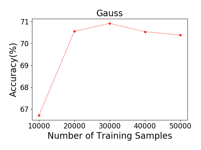
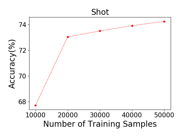
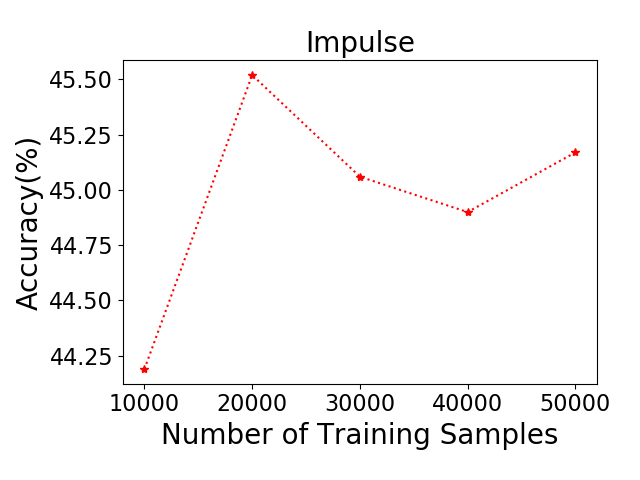
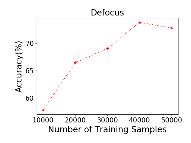
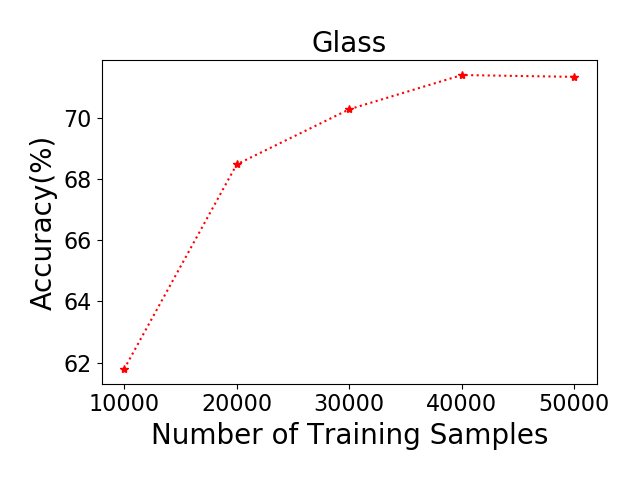
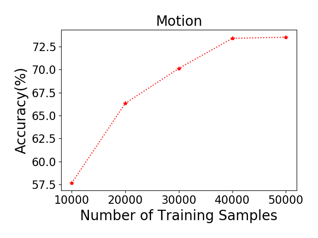
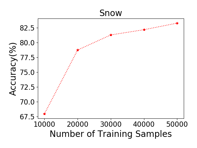
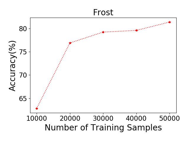
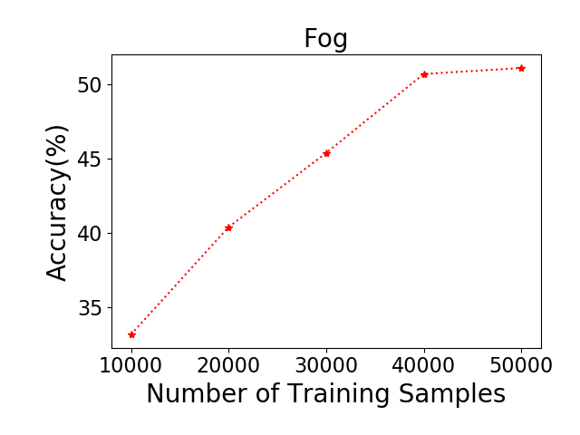
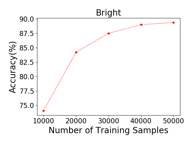
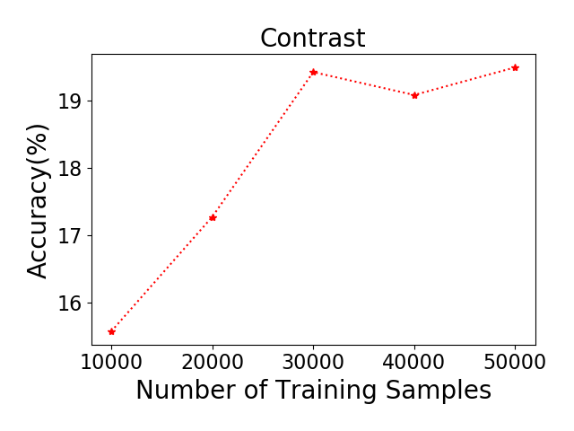
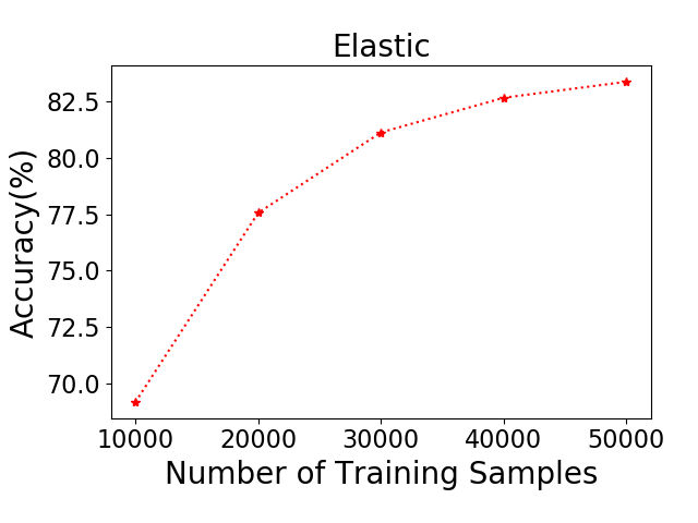
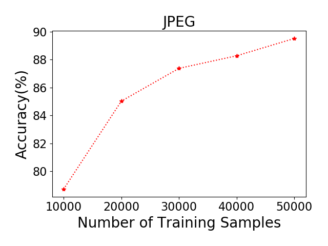
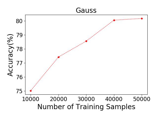
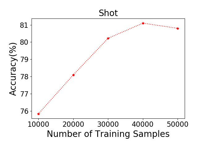
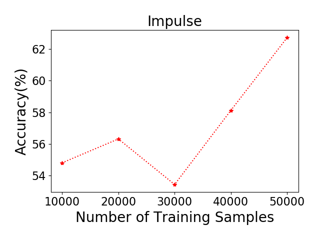
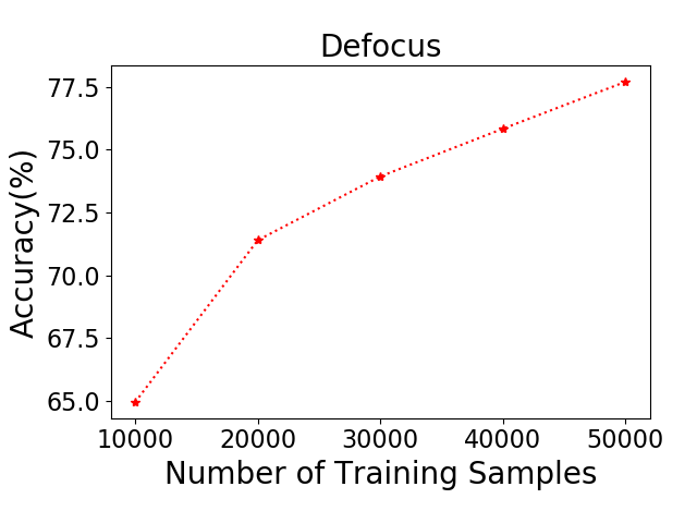
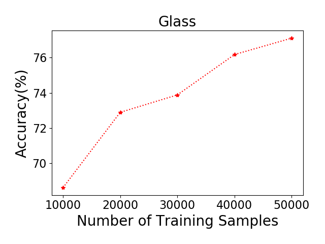
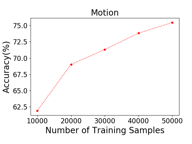
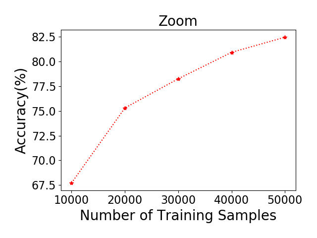
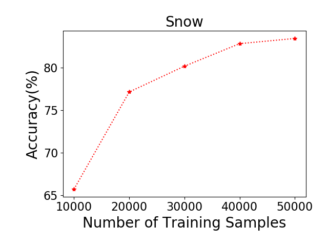
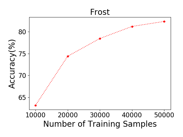
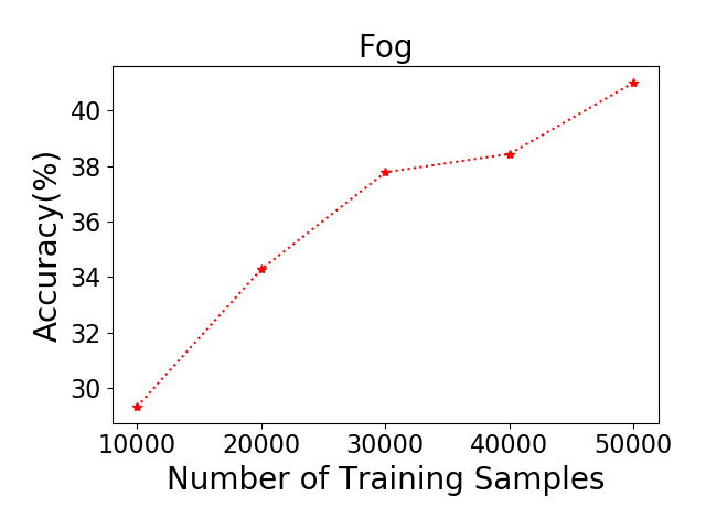
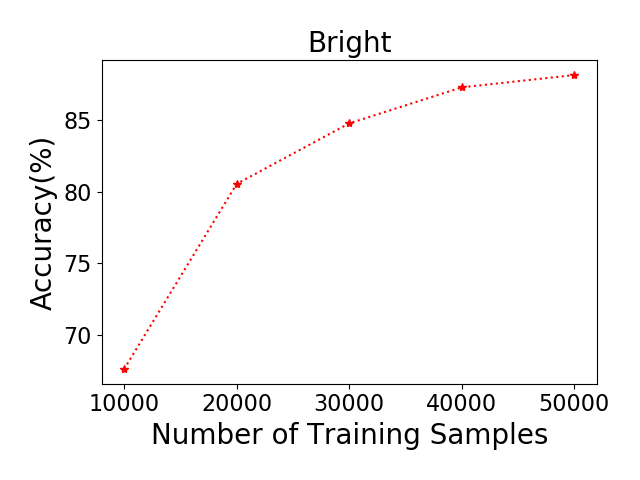
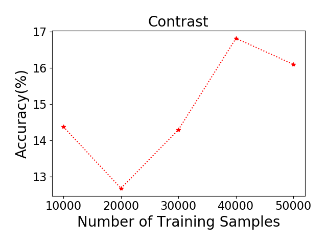
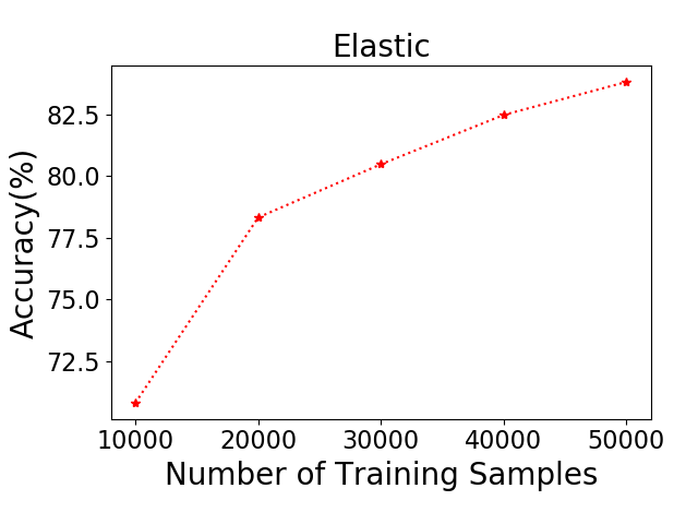
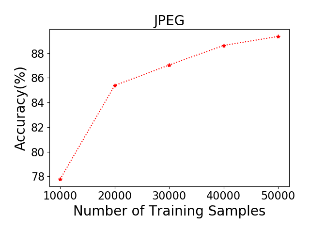
D.2 Effect of the the Number of Training Samples

We study the effect of the number of training samples, as bounds (5) and (6) suggest that more training samples lead to better OOD generalization. We split CIFAR10 into 5 subsets, each of which has 10000, 20000, 30000, 40000 and 50000 training samples. The other settings follow those in Section 5.1.1. The results are in shown Figures 5 and 6.

(a) Clean.

(b) Gauss.

(c) Shot.

(d) Impulse.

(e) Defocus.

(f) Glass.

(g) Motion.

(h) Zoom.

(i) Snow.

(j) Frost.

(k) Fog.

(l) Bright.

(m) Contrast.

(n) Elastic.

(o) pixel.

(p) JPEG.

Figure 2: 15 types of artificially constructed corruptions from four categories: Noise, Blur, Weather, and Digital from the ImageNet-C dataset (Hendrycks & Dietterich, 2018). Each corruption has five levels of severity with figures under severity 5 are shown here.

(a)

(b)

(c)

(d)

(e)

(f)

(g)

(h)

(i)

(j)

(k)

(l)

(m)

(n)

(o)

Figure 3: Accuracy of Adv-$\ell_{2}$ on CIFAR10-C over various perturbation sizes. The $x$-axis means the perturbation size is $2^{x}/12$.

(a)

(b)

(c)

(d)

(e)

(f)

(g)

(h)

(i)

(j)

(k)

(l)

(m)

(n)

(o)

Figure 4: Accuracy of Adv-$\ell_{\infty}$ on CIFAR10-C over various perturbation sizes. The $x$-axis means the perturbation size is $2^{x}/255$.

(a)

(b)

(c)

(d)

(e)

(f)

(g)

(h)

(i)

(j)

(k)

(l)

(m)

(n)

(o)

Figure 5: Accuracy of Adv-$\ell_{2}$ on CIFAR10-C over various numbers of training samples.

(a)

(b)

(c)

(d)

(e)

(f)

(g)

(h)

(i)

(j)

(k)

(l)

(m)

(n)

(o)

Figure 6: Accuracy of Adv-$\ell_{\infty}$ on CIFAR10-C over various numbers of training samples.

References

- Allen-Zhu et al. (2019) Allen-Zhu, Z., Li, Y., and Song, Z. A convergence theory for deep learning via over-parameterization. In International Conference on Machine Learning, 2019.
- Athalye et al. (2018) Athalye, A., Carlini, N., and Wagner, D. Obfuscated gradients give a false sense of security: Circumventing defenses to adversarial examples. In International Conference on Machine Learning, 2018.
- Ben-Tal et al. (2013) Ben-Tal, A., Den Hertog, D., De Waegenaere, A., Melenberg, B., and Rennen, G. Robust solutions of optimization problems affected by uncertain probabilities. Management Science, 59(2):341–357, 2013.
- Brown et al. (2020) Brown, T. B., Mann, B., Ryder, N., Subbiah, M., Kaplan, J., Dhariwal, P., Neelakantan, A., Shyam, P., Sastry, G., Askell, A., et al. Language models are few-shot learners. Preprint, 2020.
- Bubeck (2014) Bubeck, S. Convex optimization: Algorithms and complexity. Preprint arXiv:1405.4980, 2014.
- Cer et al. (2017) Cer, D., Diab, M., Agirre, E., Lopez-Gazpio, I., and Specia, L. Semeval-2017 task 1: semantic textual similarity multilingual and crosslingual focused evaluation. In International Workshop on Semantic Evaluation, 2017.
- Deng et al. (2009) Deng, J., Dong, W., Socher, R., Li, L.-J., Li, K., and Fei-Fei, L. Imagenet: A large-scale hierarchical image database. In IEEE Conference on Computer Vision and Pattern Recognition, 2009.
- Devlin et al. (2019) Devlin, J., Chang, M.-W., Lee, K., and Toutanova, K. Bert: Pre-training of deep bidirectional transformers for language understanding. In Conference of the North American Chapter of the Association for Computational Linguistics, 2019.
- Dosovitskiy et al. (2021) Dosovitskiy, A., Beyer, L., Kolesnikov, A., Weissenborn, D., Zhai, X., Unterthiner, T., Dehghani, M., Minderer, M., Heigold, G., Gelly, S., et al. An image is worth 16x16 words: Transformers for image recognition at scale. In International Conference on Learning Representations, 2021.
- Du et al. (2019) Du, S., Lee, J., Li, H., Wang, L., and Zhai, X. Gradient descent finds global minima of deep neural networks. In International Conference on Machine Learning, 2019.
- Duchi (2016) Duchi, J. Lecture notes for statistics 311/electrical engineering 377, 2016. http://web.stanford.edu/class/stats311/lecture-notes.pdf.
- Goodfellow et al. (2015) Goodfellow, I. J., Shlens, J., and Szegedy, C. Explaining and harnessing adversarial examples. In International Conference on Learning Representations, 2015.
- He et al. (2016) He, K., Zhang, X., Ren, S., and Sun, J. Deep residual learning for image recognition. In IEEE Conference on Computer Vision and Pattern Recognition, 2016.
- Hendrycks & Dietterich (2018) Hendrycks, D. and Dietterich, T. Benchmarking neural network robustness to common corruptions and perturbations. In International Conference on Learning Representations, 2018.
- Hendrycks et al. (2019) Hendrycks, D., Lee, K., and Mazeika, M. Using pre-training can improve model robustness and uncertainty. In International Conference on Machine Learning, 2019.
- Hendrycks et al. (2020a) Hendrycks, D., Basart, S., Mu, N., Kadavath, S., Wang, F., Dorundo, E., Desai, R., Zhu, T., Parajuli, S., Guo, M., et al. The many faces of robustness: A critical analysis of out-of-distribution generalization. Preprint arXiv:2006.16241, 2020a.
- Hendrycks et al. (2020b) Hendrycks, D., Liu, X., Wallace, E., Dziedzic, A., Krishnan, R., and Song, D. Pretrained transformers improve out-of-distribution robustness. In Annual Conference of the Association for Computational Linguistics, 2020b.
- Kannan et al. (2018) Kannan, H., Kurakin, A., and Goodfellow, I. Adversarial logit pairing. Preprint arXiv:1803.06373, 2018.
- Kornblith et al. (2019) Kornblith, S., Shlens, J., and Le, Q. V. Do better imagenet models transfer better? In IEEE Conference on Computer Vision and Pattern Recognition, 2019.
- Krizhevsky & Hinton (2009) Krizhevsky, A. and Hinton, G. Learning multiple layers of features from tiny images. 2009.
- Lee & Raginsky (2018) Lee, J. and Raginsky, M. Minimax statistical learning with wasserstein distances. In Advances in Neural Information Processing Systems, 2018.
- Li et al. (2020) Li, Y., Fang, E. X., Xu, H., and Zhao, T. Inductive bias of gradient descent based adversarial training on separable data. In International Conference on Learning Representations, 2020.
- Liu et al. (2020) Liu, C., Zhu, L., and Belkin, M. Toward a theory of optimization for over-parameterized systems of non-linear equations: the lessons of deep learning. Preprint arXiv:2003.00307, 2020.
- Liu et al. (2019) Liu, Y., Ott, M., Goyal, N., Du, J., Joshi, M., Chen, D., Levy, O., Lewis, M., Zettlemoyer, L., and Stoyanov, V. Roberta: A robustly optimized bert pretraining approach. Preprint arXiv:1907.11692, 2019.
- Lohn (2020) Lohn, A. J. Estimating the brittleness of ai: safety integrity levels and the need for testing out-of-distribution performance. Preprint arXiv:2009.00802, 2020.
- Loshchilov & Hutter (2018) Loshchilov, I. and Hutter, F. Decoupled weight decay regularization. In International Conference on Learning Representations, 2018.
- Lyu & Li (2019) Lyu, K. and Li, J. Gradient descent maximizes the margin of homogeneous neural networks. In International Conference on Learning Representations, 2019.
- Maas et al. (2011) Maas, A., Daly, R. E., Pham, P. T., Huang, D., Ng, A. Y., and Potts, C. Learning word vectors for sentiment analysis. In Annual Conference of the Association for Computational Linguistics, 2011.
- Madry et al. (2018) Madry, A., Makelov, A., Schmidt, L., Tsipras, D., and Vladu, A. Towards deep learning models resistant to adversarial attacks. In International Conference on Learning Representations, 2018.
- Namkoong (2019) Namkoong, H. Reliable machine learning via distributional robustness. PhD thesis, Stanford University, 2019.
- Nouiehed et al. (2019) Nouiehed, M., Sanjabi, M., Huang, T., Lee, J. D., and Razaviyayn, M. Solving a class of non-convex min-max games using iterative first order methods. In Advances in Neural Information Processing Systems, 2019.
- Radford et al. (2021) Radford, A., Kim, J. W., Hallacy, C., Ramesh, A., Goh, G., Agarwal, S., Sastry, G., Askell, A., Mishkin, P., Clark, J., et al. Learning transferable visual models from natural language supervision, 2021. https://openai.com/blog/clip/.
- Raghunathan et al. (2019) Raghunathan, A., Xie, S. M., Yang, F., Duchi, J. C., and Liang, P. Adversarial training can hurt generalization. Preprint arXiv:1906.06032, 2019.
- Rakhlin et al. (2012) Rakhlin, A., Shamir, O., and Sridharan, K. Making gradient descent optimal for strongly convex stochastic optimization. In International Coference on Machine Learning, 2012.
- Recht et al. (2019) Recht, B., Roelofs, R., Schmidt, L., and Shankar, V. Do imagenet classifiers generalize to imagenet? In International Conference on Machine Learning, 2019.
- Salman et al. (2020a) Salman, H., Ilyas, A., Engstrom, L., Kapoor, A., and Madry, A. Do adversarially robust imagenet models transfer better? Preprint arXiv:2007.08489, 2020a.
- Salman et al. (2020b) Salman, H., Ilyas, A., Engstrom, L., Vemprala, S., Madry, A., and Kapoor, A. Unadversarial examples: designing objects for robust vision. Preprint arXiv:2012.12235, 2020b.
- Schneider et al. (2020) Schneider, S., Rusak, E., Eck, L., Bringmann, O., Brendel, W., and Bethge, M. Improving robustness against common corruptions by covariate shift adaptation. In Advances in Neural Information Processing Systems, 2020.
- Shapiro (2017) Shapiro, A. Distributionally robust stochastic programming. SIAM Journal on Optimization, 27(4):2258–2275, 2017.
- Sinha et al. (2018) Sinha, A., Namkoong, H., and Duchi, J. Certifying some distributional robustness with principled adversarial training. In International Conference on Learning Representations, 2018.
- Socher et al. (2013) Socher, R., Perelygin, A., Wu, J., Chuang, J., Manning, C. D., Ng, A. Y., and Potts, C. Recursive deep models for semantic compositionality over a sentiment treebank. In Conference on Empirical Methods in Natural Language Processing, 2013.
- Soudry et al. (2018) Soudry, D., Hoffer, E., Nacson, M. S., Gunasekar, S., and Srebro, N. The implicit bias of gradient descent on separable data. The Journal of Machine Learning Research, 19(1):2822–2878, 2018.
- Szegedy et al. (2013) Szegedy, C., Zaremba, W., Sutskever, I., Bruna, J., Erhan, D., Goodfellow, I., and Fergus, R. Intriguing properties of neural networks. Preprint arXiv:1312.6199, 2013.
- Tu et al. (2020) Tu, L., Lalwani, G., Gella, S., and He, H. An empirical study on robustness to spurious correlations using pre-trained language models. Transactions of the Association for Computational Linguistics, 8:621–633, 2020.
- Utrera et al. (2021) Utrera, F., Kravitz, E., Erichson, N. B., Khanna, R., and Mahoney, M. W. Adversarially-trained deep nets transfer better. In International Conference on Learning Representations, 2021.
- van der Vaart & Wellner (2000) van der Vaart, A. W. and Wellner, J. A. Weak convergence and empirical processes. Springer series in statistics. Springer, 2000.
- Vershynin (2018) Vershynin, R. High-dimensional probability: an introduction with applications in data science. Cambridge Series in Statistical and Probabilistic Mathematics. Cambridge University Press, 2018.
- Villani (2008) Villani, C. Optimal transport: old and new, volume 338. Springer Science & Business Media, 2008.
- Volpi et al. (2018) Volpi, R., Namkoong, H., Sener, O., Duchi, J. C., Murino, V., and Savarese, S. Generalizing to unseen domains via adversarial data augmentation. In Advances in Neural Information Processing Systems, 2018.
- Wainwright (2019) Wainwright, M. J. High-dimensional statistics: a non-asymptotic viewpoint. Cambridge Series in Statistical and Probabilistic Mathematics. Cambridge University Press, 2019.
- Wang et al. (2018) Wang, A., Singh, A., Michael, J., Hill, F., Levy, O., and Bowman, S. R. Glue: A multi-task benchmark and analysis platform for natural language understanding. In International Conference on Learning Representations, 2018.
- Williams et al. (2018) Williams, A., Nangia, N., and Bowman, S. A broad-coverage challenge corpus for sentence understanding through inference. In Conference of the North American Chapter of the Association for Computational Linguistics, 2018.
- Wolf et al. (2020) Wolf, T., Chaumond, J., Debut, L., Sanh, V., Delangue, C., Moi, A., Cistac, P., Funtowicz, M., Davison, J., Shleifer, S., et al. Transformers: State-of-the-art natural language processing. In Conference on Empirical Methods in Natural Language Processing, 2020.
- Xie et al. (2017) Xie, B., Liang, Y., and Song, L. Diversity leads to generalization in neural networks. In International Conference on Artificial Intelligence and Statistics, 2017.
- Xie et al. (2020) Xie, C., Tan, M., Gong, B., Wang, J., Yuille, A. L., and Le, Q. V. Adversarial examples improve image recognition. In IEEE Conference on Computer Vision and Pattern Recognition, 2020.
- Xu & Mannor (2012) Xu, H. and Mannor, S. Robustness and generalization. Machine learning, 86(3):391–423, 2012.
- Yin et al. (2019) Yin, D., Kannan, R., and Bartlett, P. Rademacher complexity for adversarially robust generalization. In International Conference on Machine Learning, 2019.
- Zhu et al. (2019) Zhu, C., Cheng, Y., Gan, Z., Sun, S., Goldstein, T., and Liu, J. Freelb: Enhanced adversarial training for natural language understanding. In International Conference on Learning Representations, 2019.