Transport Synthetic Acceleration for the Solution of the One-Speed
Nonclassical Spectral S_N Equations in Slab Geometry

Abstract

The nonclassical transport equation models particle transport processes in which the particle flux does not decrease as an exponential function of the particle’s free-path. Recently, a spectral approach was developed to generate nonclassical spectral S_N equations, which can be numerically solved in a deterministic fashion using classical numerical techniques. This paper introduces a transport synthetic acceleration procedure to speed up the iteration scheme for the solution of the monoenergetic slab-geometry nonclassical spectral S_N equations. We present numerical results that confirm the benefit of the acceleration procedure for this class of problems.

1 Introduction

In the classical theory of linear particle transport, the incremental probability that a particle at position ${\bm{x}}=(x,y,z)$ will experience a collision while traveling an incremental distance $ds$ in the background material is given by

$$dp=\sigma_{t}({\bm{x}})ds\,,$$ (1.1)

where $\sigma_{t}$ represents the macroscopic total cross section [1]. The implicit assumption is that $\sigma_{t}$ is independent of the particle’s direction-of-flight ${\bf\Omega}$ and of the particle’s free-path $s$, defined as the distance traveled by the particle since its previous interaction (birth or scattering). This assumption leads to the particle flux being exponentially attenuated (Beer-Lambert law). We remark that extending the results discussed here to include energy- or frequency-dependence is straightforward.

The theory of nonclassical particle transport employs a generalized form of the linear Boltzmann equation to model processes in which the particle flux is not attenuated exponentially. This area has been significantly researched in recent years [2, 3, 4, 5, 6, 7, 8, 9, 10, 11, 12, 13, 14, 15]. Originally introduced to describe photon transport in the Earth’s cloudy atmosphere [16, 17, 18, 19, 20, 21], it has found its way to other applications, including nuclear engineering [22, 23, 24, 25, 26] and computer graphics [27, 28, 29]. Furthermore, an analogous theory yielding a similar kinetic equation has been independently derived for the periodic Lorentz gas by Marklof and Strömbergsson [30, 31, 32, 33] and by Golse (cf. [34]).

The nonclassical transport equation allows the nonclassical macroscopic total cross section $\Sigma_{t}$ to be a function of the particle’s free-path, and is defined in an extended phase space that includes $s$ as an independent variable. If we define

$$P({\bm{x}},{\bf\Omega},s)ds=\left(\begin{array}[]{l}\text{the probability that a particle released at position ${\bm{x}}$ in the}\\ \text{direction ${\bf\Omega}$ will experience its next collision while traveling}\\ \text{an incremental interval between $s$ and $s+ds$}\end{array}\right)\,,$$ (1.5)

then we can define the ensemble average

$$p(s)=\left<P({\bm{x}},{\bf\Omega},s)\right>_{({\bm{x}},{\bf\Omega},\mathcal{R})}$$ (1.6)

over all “release positions” ${\bm{x}}$ in a realization of the system, all directions ${\bf\Omega}$, and all possible realizations $\mathcal{R}$. In this case, $p(s)$ represents the free-path distribution function, and the nonclassical cross section $\Sigma_{t}(s)$ satisfies

$$p(s)=\Sigma_{t}(s)e^{-\int_{0}^{s}\Sigma_{t}(s^{\prime})ds^{\prime}}\,.$$ (1.7)

It is possible to extend this definition to include angular-dependent free-path distributions and cross sections [5], but in this paper we will restrict ourselves to the case given by Eq. 1.7.

The steady-state, one-speed nonclassical transport equation with isotropic scattering can be written as [3]

$$\frac{\partial}{\partial s}\Psi({\bm{x}},{\bf\Omega},s)+{\bf\Omega}\cdot{\bf\nabla}\Psi({\bm{x}},{\bf\Omega},s)+\Sigma_{t}(s)\Psi({\bm{x}},{\bf\Omega},s)=$$ (1.8a)

$$\qquad\qquad\delta(s)\left[\frac{c}{4\pi}\int_{4\pi}\int_{0}^{\infty}\Sigma_{t}(s^{\prime})\Psi({\bm{x}},{\bf\Omega}^{\prime},s^{\prime})ds^{\prime}d\Omega^{\prime}+\frac{Q({\bm{x}})}{4\pi}\right]\,,\hskip 5.0pt{\bm{x}}\in V,\,\,{\bf\Omega}\in 4\pi,\,\,0<s,$$

where $$\Psi c Q \delta(s) s=0$$ is the nonclassical angular flux, is the scattering ratio, and is an isotropic internal source. The Dirac delta function on the right-hand side of Eq. 1.8a represents the fact that a particle that has just undergone scattering or been born will have its free-path value (distance since previous interaction) set to . If we consider vacuum boundaries, Eq. 1.8a is subject to the boundary condition

$$\Psi({\bm{x}},{\bf\Omega},s)=0\,,\quad{\bm{x}}\in\partial V,\,\,{\bm{n}}\cdot{\bf\Omega}<0,\,\,0<s\,.$$ (1.8b)

We remark that, if $\Sigma_{t}(s)$ is assumed to be independent of $s$, then $\Sigma_{t}(s)=\sigma_{t}$ and the free-path distribution in Eq. 1.7 reduces to the exponential

$$p(s)=\sigma_{t}e^{-\sigma_{t}s}\,.$$ (1.9)

In this case, Eq. 1.8a can be shown to reduce to the corresponding classical linear Boltzmann equation

$${\bf\Omega}\cdot{\bf\nabla}\Psi_{c}({\bm{x}},{\bf\Omega})+\sigma_{t}\Psi_{c}({\bm{x}},{\bf\Omega})=\frac{c}{4\pi}\int_{4\pi}\sigma_{t}\Psi_{c}({\bm{x}},{\bf\Omega}^{\prime})d\Omega^{\prime}+\frac{Q({\bm{x}})}{4\pi}\,,\hskip 10.0pt{\bm{x}}\in V,\,\,{\bf\Omega}\in 4\pi\,,$$ (1.10a)

with vacuum boundary condition given by

$$\Psi_{c}({\bm{x}},{\bf\Omega})=0\,,\quad{\bm{x}}\in\partial V,\,\,{\bm{n}}\cdot{\bf\Omega}<0\,.$$ (1.10b)

Here, the classical angular flux $\Psi_{c}$ is given by

$$\Psi_{c}({\bm{x}},{\bf\Omega})=\int_{0}^{\infty}\Psi({\bm{x}},{\bf\Omega},s)ds\,.$$ (1.11)

Recently, a spectral approach was developed to represent the nonclassical flux as a series of Laguerre polynomials in the variable $s$ [35]. The resulting equation has the form of a classical transport equation that can be solved in a deterministic fashion using traditional methods. Specifically, the nonclassical solution was obtained using the conventional discrete ordinates (S_N) formulation [36] and a source iteration (SI) scheme [37]. However, for highly scattering systems the spectral radius of the transport problem can get arbitrarily close to unity [36], and numerical acceleration becomes important.

The goal of this paper is to introduce transport synthetic acceleration techniques–namely, S₂ synthetic acceleration (S₂SA)–to speed up the solution of the nonclassical spectral S_N equations. We also present numerical results that confirm the benefit of using this approach; to our knowledge, this is the first time such acceleration methods are applied to this class of nonclassical spectral problems.

The remainder of the paper is organized as follows. In Section 2, we present the nonclassical spectral S_N equations for slab geometry. We discuss transport synthetic acceleration in Section 3 and present an iterative method to efficiently solve the nonclassical problem. Numerical results are given in Section 4 for problems with both exponential (Section 4.1) and nonexponential (Section 4.2) choices of $p(s)$. We conclude with a brief discussion in Section 5.

2 Nonclassical Spectral S_N Equations in Slab Geometry

In this section we briefly sketch out the derivation of the one-speed nonclassical spectral S_N equations in slab geometry. For a detailed derivation, we direct the reader to the work presented in [35].

In slab geometry, Eq. 1.8 can be written as

$$\frac{\partial}{\partial s}\Psi(x,\mu,s)+\mu\frac{\partial}{\partial x}\Psi(x,\mu,s)+\Sigma_{t}(s)\Psi(x,\mu,s)=$$ (2.1a)

$$\qquad\delta(s)\left[\frac{c}{2}\int_{-1}^{1}\int_{0}^{\infty}\Sigma_{t}(s^{\prime})\Psi(x,\mu^{\prime},s^{\prime})ds^{\prime}d\mu^{\prime}+\frac{Q(x)}{2}\right]\,,\hskip 5.0pt0<x<X,\,\,-1<\mu<1,\,\,0<s,$$

$$\Psi(0,\mu,s)=0\,,\quad 0<\mu\leq 1\,,0<s\,,$$ (2.1b)

$$\Psi(X,\mu,s)=0\,,\quad-1\leq\mu<0\,,0<s\,,$$ (2.1c)

where $\mu$ is the cosine of the scattering angle. Equation 2.1a can be written in an equivalent “initial value” form:

$$\frac{\partial}{\partial s}\Psi(x,\mu,s)+\mu\frac{\partial}{\partial x}\Psi(x,\mu,s)+\Sigma_{t}(s)\Psi(x,\mu,s)=0\,,$$ (2.2a)

$$\Psi(x,\mu,0)=\frac{c}{2}\int_{-1}^{1}\int_{0}^{\infty}\Sigma_{t}(s^{\prime})\Psi(x,\mu^{\prime},s^{\prime})ds^{\prime}d\mu^{\prime}+\frac{Q(x)}{2}\,.$$ (2.2b)

Note that, due to scattering and internal source being isotropic, the right-hand side of Eq. 2.2b does not depend on $\mu$.

Defining $\psi$ such that

$$\Psi(x,\mu,s)\equiv\psi(x,\mu,s)e^{-\int_{0}^{s}\Sigma_{t}(s^{\prime})ds^{\prime}}\,,$$ (2.3)

we can rewrite the nonclassical problem as

$$\frac{\partial}{\partial s}\psi(x,\mu,s)+\mu\frac{\partial}{\partial x}\psi(x,\mu,s)=0,$$ (2.4a)

$$\psi(x,\mu,0)=\frac{c}{2}\int_{-1}^{1}\int_{0}^{\infty}p(s^{\prime})\psi(x,\mu^{\prime},s^{\prime})ds^{\prime}d\mu^{\prime}+\frac{Q(x)}{2}\,,$$ (2.4b)

where $$p(s)$$ is given by Eq. 1.7. This problem has the vacuum boundary conditions

$$\psi(0,\mu,s)=0\,,\quad 0<\mu\leq 1\,,0<s\,,$$ (2.4c)

$$\psi(X,\mu,s)=0\,,\quad-1\leq\mu<0\,,0<s\,.$$ (2.4d)

Next, we write $\psi$ as a truncated series of Laguerre polynomials in $s$:

$$\psi(x,\mu,s)=\sum_{m=0}^{M}\psi_{m}(x,\mu)L_{m}(s),$$ (2.5)

where $L_{m}(s)$ is the Laguerre polynomial of order $m$ and $M$ is the expansion (truncation) order. The Laguerre polynomials $\{L_{m}(s)\}$ are orthogonal with respect to the weight function $e^{-s}$ and satisfy $\frac{d}{ds}L_{m}(s)=\left(\frac{d}{ds}-1\right)L_{m-1}(s)$ for $m>0$ [38]. We introduce this expansion in the nonclassical problem and perform the following steps [35]: (i) multiply Eq. 2.4a by $e^{-s}L_{m}(s)$; (ii) integrate from $0$ to $\infty$ with respect to $s$; and (iii) use the properties of the Laguerre polynomials to simplify the result. This procedure returns the following nonclassical spectral problem:

$$\mu\frac{\partial}{\partial x}\psi_{m}(x,\mu)+\psi_{m}(x,\mu)=S(x)+\frac{Q(x)}{2}-\sum_{j=0}^{m-1}\psi_{j}(x,\mu),\quad m=0,1,...,M\,,$$ (2.6a)

$$\psi_{m}(0,\mu)=0\,,\quad 0<\mu\leq 1\,,m=0,1,...,M\,,$$ (2.6b)

$$\psi_{m}(X,\mu)=0\,,\quad-1\leq\mu<0\,,m=0,1,...,M\,,$$ (2.6c)

where the in-scattering term $$S(x)$$ (the scattering source) is given by

$$S(x)=\frac{c}{2}\int_{-1}^{1}\sum_{k=0}^{M}\psi_{k}(x,\mu^{\prime})\left[\int_{0}^{\infty}p(s)L_{k}(s)ds\right]d\mu^{\prime}\,.$$ (2.6d)

The nonclassical angular flux $\Psi$ is recovered from Eqs. 2.3 and 2.5. The classical angular flux $\Psi_{c}$ is obtained using Eq. 1.11, such that

$$\Psi_{c}(x,\mu)=\int_{0}^{\infty}\Psi(x,\mu,s)ds=\sum_{m=0}^{M}\psi_{m}(x,\mu)\int_{0}^{\infty}L_{m}(s)e^{-\int_{0}^{s}\Sigma_{t}(s^{\prime})ds^{\prime}}ds\,.$$ (2.7)

Finally, using the discrete ordinates formulation [36], we can write the nonclassical spectral S_N equations

$$\mu_{n}\frac{d}{dx}\psi_{m,n}(x)+\psi_{m,n}(x)=S(x)+\frac{Q(x)}{2}-\sum_{j=0}^{m-1}\psi_{j,n}(x),$$ (2.8a)

$$\hskip 250.0ptm=0,1,...,M,\,n=1,2,...,N\,,$$

$$\psi_{m,n}(0)=0\,,\quad m=0,1,...,M,\,n=1,2,...,\frac{N}{2}\,,$$ (2.8b)

$$\psi_{m,n}(X)=0\,,\quad m=0,1,...,M,\,n=\frac{N}{2}+1,...,N\,,$$ (2.8c)

$$S(x)=\frac{c}{2}\sum_{n=1}^{N}\omega_{n}\sum_{k=0}^{M}\psi_{k,n}(x)\left[\int_{0}^{\infty}p(s)L_{k}(s)ds\right]\,,$$ (2.8d)

$$\Psi_{c_{n}}(x)=\sum_{m=0}^{M}\psi_{m,n}(x)\int_{0}^{\infty}L_{m}(s)e^{-\int_{0}^{s}\Sigma_{t}(s^{\prime})ds^{\prime}}ds\,,\quad n=1,2,...,N\,.$$ (2.8e)

Here, the cosine of the scattering angle $\mu$ has been discretized in $N$ discrete values $\mu_{n}$. Thus, $\psi_{m,n}(x)=\psi_{m}(x,\mu_{n})$, $\Psi_{c_{n}}(x)=\Psi_{c}(x,\mu_{n})$, and the angular integral has been approximated by the angular quadrature formula with weights $\omega_{n}$.

3 Source Iteration and Synthetic Acceleration

To solve the nonclassical spectral S_N equations using standard source iteration [37], we lag the scattering source on the right-hand side of Eq. 2.8a:

$$\mu_{n}\frac{d}{dx}\psi_{m,n}^{i+1}(x)+\psi_{m,n}^{i+1}(x)=S^{i}(x)+\frac{Q(x)}{2}-\sum_{j=0}^{m-1}\psi_{j,n}^{i+1}(x),$$ (3.1a)

where $$i$$ is the iteration index and

$$S^{i}(x)=\frac{c}{2}\sum_{n=1}^{N}\omega_{n}\sum_{k=0}^{M}\psi_{k,n}^{i}(x)\left[\int_{0}^{\infty}p(s)L_{k}(s)ds\right]\,.$$ (3.1b)

In order to accelerate the convergence of this approach, the iterative scheme is broken into multiple stages.

Standard synthetic acceleration methods consist of two stages. The first stage is a single transport sweep. The second stage is error-correction, which uses an approximation of the error equation to estimate the error at each iteration. Our synthetic acceleration scheme has the following steps:

• Determine the new “half iterate” $\psi^{i+\frac{1}{2}}$ (solution estimate) using one transport sweep.

  This is done by solving

  $$\mu_{n}\frac{d}{dx}\psi_{m,n}^{i+\frac{1}{2}}(x)+\psi_{m,n}^{i+\frac{1}{2}}(x)=S^{i}(x)+\frac{Q(x)}{2}-\sum_{j=0}^{m-1}\psi_{j,n}^{i+\frac{1}{2}}(x).$$ (3.2)

• Approximate the error $\epsilon^{i+1}$ in this half iterate using an approximation to the error equation (error estimate).

  To do that, we first subtract Eq. 3.2 from the exact equation Eq. 2.8a, then add and subtract $\psi_{k,n}^{i+\frac{1}{2}}(x)$ to the in-scattering term on the right-hand side. This yields

  $$\mu_{n}\frac{d}{dx}\left(\psi_{m,n}(x)-\psi_{m,n}^{i+\frac{1}{2}}(x)\right) +\left(\psi_{m,n}(x)-\psi_{m,n}^{i+\frac{1}{2}}(x)\right)=$$ (3.3a)

  $$\qquad\qquad\left(S(x)-S^{i}(x)\right)-\sum_{j=0}^{m-1}\left(\psi_{j,n}(x)-\psi_{j,n}^{i+\frac{1}{2}}(x)\right)\,,$$

  where

  $$S(x)-S^{i}(x)=\frac{c}{2}\sum_{n=1}^{N}\omega_{n}\sum_{k=0}^{M} \left(\psi_{k,n}(x)-\psi_{k,n}^{i+\frac{1}{2}}(x)+\right.$$ (3.3b)

  $$\qquad\qquad\left.\psi_{k,n}^{i+\frac{1}{2}}(x)-\psi_{k,n}^{i}(x)\right)\left[\int_{0}^{\infty}p(s)L_{k}(s)ds\right]\,.$$

  Defining the error $\epsilon^{i+1}_{m,n}$ as

  $$\epsilon^{i+1}_{m,n}(x)\equiv\psi_{m,n}(x)-\psi_{m,n}^{i+\frac{1}{2}}(x)\,,$$ (3.4)

  we rewrite Eq. 3.3 as

  $$\mu_{n}\frac{d}{dx}\epsilon^{i+1}_{m,n}(x)+\epsilon^{i+1}_{m,n}(x)-S^{{i+1},\epsilon}(x)=\left(S^{i+\frac{1}{2}}(x)-S^{i}(x)\right)-\sum_{j=0}^{m-1}\epsilon^{i+1}_{j,n}(x)\,,$$ (3.5a)

  with

  $$S^{{i+1},\epsilon}(x)=\frac{c}{2}\sum_{n=1}^{N}\omega_{n}\sum_{k=0}^{M}\epsilon^{i+1}_{k,n}(x)\left[\int_{0}^{\infty}p(s)L_{k}(s)ds\right]\,.$$ (3.5b)

  We solve Eq. 3.5 and obtain the error estimate $\epsilon^{i+1}$.

• Correct the solution estimate using the error estimate.

  The corrected solution estimate $\psi^{i+1}$ is given by

  $$\psi^{i+1}_{m,n}(x)=\psi^{i+\frac{1}{2}}_{m,n}(x)+\epsilon^{i+1}_{m,n}(x)\,.$$ (3.6)

• Check for convergence and loop back if necessary.

We remark that this transport synthetic acceleration procedure accelerates each one of the $M$ Laguerre moments of the angular flux. In this paper, we have chosen to approximate the error estimate in Eq. 3.5 by setting $N=2$, thus applying S₂ synthetic acceleration (S₂SA).

4 Numerical Results

In this section we provide numerical results that confirm the benefit of using transport synthetic acceleration for the iterative numerical solution of the nonclassical spectral S_N equations (2.8). For validation purposes, we first apply this nonclassical approach to solve a transport problem with an exponential $p(s)$, which leads to classical transport. Then, we proceed to solve a nonclassical transport problem that mimics diffusion, with a nonexponential $p(s)$.

For all numerical experiments in this section we use the Gauss-Legendre angular quadrature [39] with $N=16$ for Eq. 2.8 and $N=2$ for Eq. 3.5, thus solving the nonclassical spectral S₁₆ equations using S₂ synthetic acceleration. We discretize the spatial variable into 200 elements and use the linear discontinuous Galerkin finite element method [40]. Furthermore, the improper integrals $\int_{0}^{\infty}(\cdot)ds$ in these equations are calculated numerically in the same fashion as in [35]: the upper limit is truncated to $1.5$ times the length of the slab, and a Gauss-Legendre quadrature is used to solve them. Here, we set the order of this quadrature to $M$, the same order as the Laguerre expansion.

The stopping criterion adopted is that the relative deviations between two consecutive estimates of the classical scalar flux

$$\Phi(x)=\sum_{n=1}^{N}\omega_{n}\Psi_{c_{n}}(x)$$ (4.1)

in each point of the spatial discretization grid need to be smaller than or equal to a prescribed positive constant $\xi$. For all our calculations we fix $\xi=10^{-6}$, such that the stopping criterion is given by

$$\frac{||\Phi^{i+1}(x)-\Phi^{i}(x)||}{||\Phi^{i}(x)||}\leq\xi\,.$$ (4.2)

4.1 Exponential $p(s)$

To validate the approach, we use the nonclassical method to solve a transport problem in which $p(s)$ is given by the exponential function provided in Eq. 1.9. This yields [3]

$$\Sigma_{t}(s)=\frac{p(s)}{\int_{s}^{\infty}p(s^{\prime})ds^{\prime}}=\frac{\sigma_{t}e^{-\sigma_{t}s}}{\int_{s}^{\infty}\sigma_{t}e^{-\sigma_{t}s^{\prime}}ds^{\prime}}=\sigma_{t}\text{ (independent of $s$).}$$ (4.3)

In this case, the flux $\Psi_{c_{n}}$ given by Eq. 2.8e should match the one obtained by solving the corresponding classical S_N transport problem

$$\mu_{n}\frac{d}{dx}\Psi_{c_{n}}(x)+\sigma_{t}\Psi_{c_{n}}(x)=\frac{c}{2}\sigma_{t}\sum_{n=1}^{N}\omega_{n}\Psi_{c_{n}}(x)+\frac{Q(x)}{2}\,,\quad 0<x<X\,,n=1,2,...,N\,,$$ (4.4a)

$$\Psi_{c_{n}}(0)=0\,,\quad n=1,2,...,\frac{N}{2}\,,$$ (4.4b)

$$\Psi_{c_{n}}(X)=0\,,\quad n=\frac{N}{2}+1,...,N\,.$$ (4.4c)

Let us consider a slab of length $X=20$, total cross section $\sigma_{t}=1.0$, scattering ratio $c=0.999$, and internal source $Q(x)=1.0$, and let us assume the truncation order of the Laguerre expansion to be $M=10$. Figure 1 depicts the scalar flux obtained when solving the nonclassical (2.8) and classical (4.4) problems. As expected, the solutions match each other.

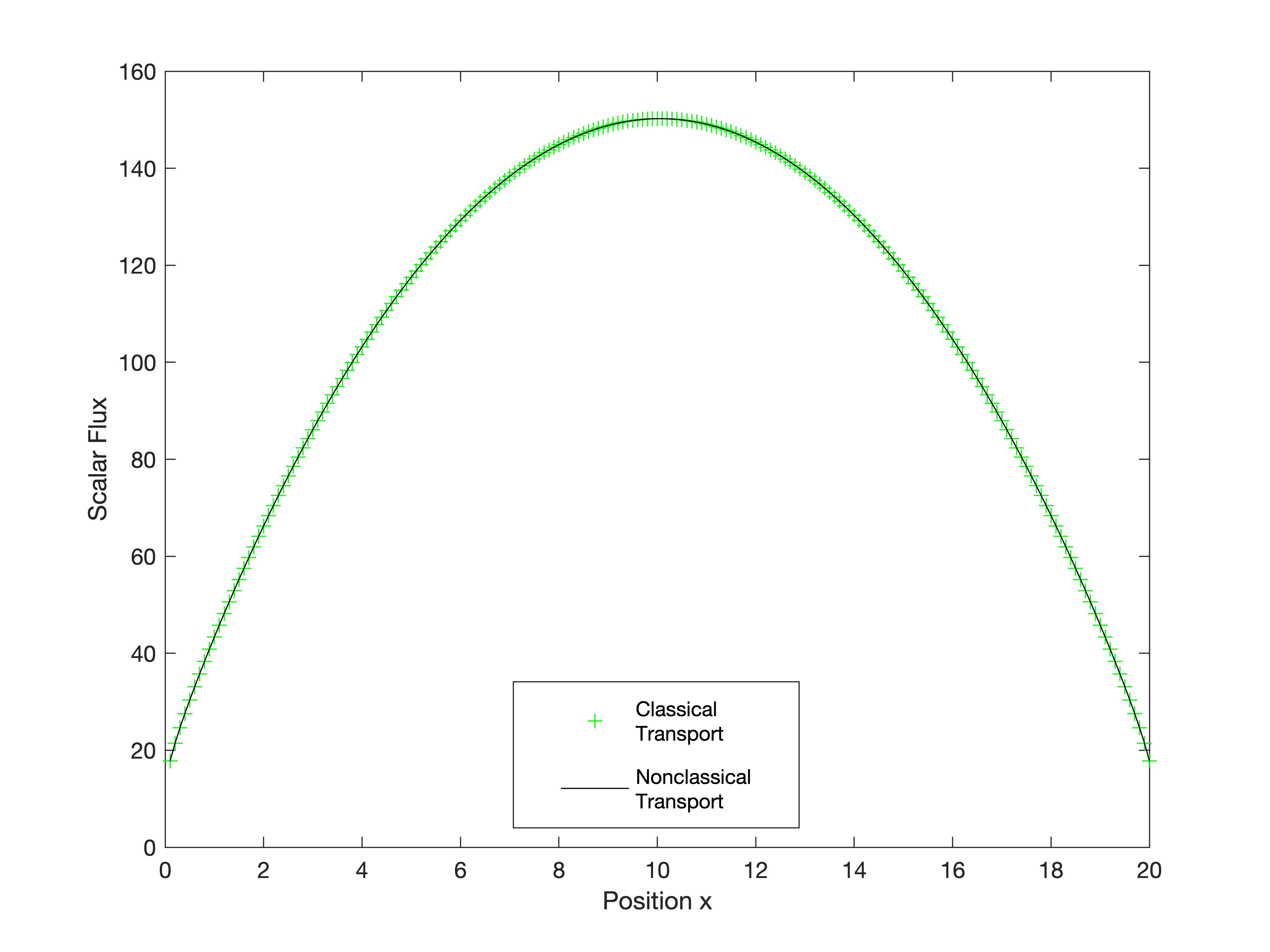
Figure 1: Scalar flux generated by the solution of classical and nonclassical transport equations

Table 1: Convergence Data for Nonclassical Transport with Exponential $p(s)$

	Number of		Spectral
	Iterations		Radius
$\mathbf{c}$	SI	S2SA	SI	S2SA
0.8	56	6	0.7997	0.1328
0.9	110	6	0.8997	0.1565
0.99	906	6	0.9899	0.1748
0.999	6439	6	0.9989	0.1685

Next, we compare the iteration count and spectral radius for stand-alone source iteration (SI) and transport synthetic acceleration (S₂SA) for the nonclassical method. Once again, we set $Q(x)=1.0$, and $p(s)$ and $\Sigma_{t}(s)$ are given respectively by Eqs. (1.9) and (4.3), with $\sigma_{t}=1.0$. However, this time we increase the domain size to $X=200$. We assume the truncation order of the Laguerre expansion to be $M=50$, and vary the scattering ratio $c$ from 0.8 to 0.999. Table 1 presents the number of iterations and the spectral radius for each case. As expected, we observe a significant reduction in the spectral radius and iteration count, with the number of iterations decreasing 3 orders of magnitude for the highest scattering ratio of $c=0.999$.

4.2 Nonexponential $p(s)$

Let us consider the diffusion equation in a homogeneous slab

$$-\frac{1}{3\sigma_{t}}\frac{d^{2}}{dx^{2}}\phi(x)+(1-c)\sigma_{t}\phi(x)=Q(x)\,,$$ (4.5a)

with Marshak boundary conditions [41]

$$\phi(0)-\frac{2}{3\sigma_{t}}\frac{d}{dx}\phi(0)=0\,,$$ (4.5b)

$$\phi(X)+\frac{2}{3\sigma_{t}}\frac{d}{dx}\phi(X)=0\,.$$ (4.5c)

Here, $\phi$ is the (diffusion) scalar flux.

If the free-path distribution $p(s)$ is given by the nonexponential function

$$p(s)=3\sigma_{t}^{2}s\,e^{-\sqrt{3}\sigma_{t}s},$$ (4.6)

it has been shown that the collision-rate density $\sigma_{t}\phi(x)$ of the diffusion problem, given by Eq. 4.5, will match the nonclassical collision-rate density [7, 8]

$$f(x)=\int_{0}^{\infty}\Sigma_{t}(s)\int_{-1}^{1}\Psi(x,\mu,s)d\mu ds,$$ (4.7)

where $\Psi(x,\mu,s)$ is the solution of the nonclassical problem given by Eq. 2.1, and

$$\Sigma_{t}(s)=\frac{p(s)}{\int_{s}^{\infty}p(s^{\prime})ds^{\prime}}=\frac{3\sigma_{t}^{2}se^{-\sqrt{3}\sigma_{t}s}}{\int_{s}^{\infty}3\sigma_{t}^{2}s^{\prime}e^{-\sqrt{3}\sigma_{t}s^{\prime}}ds^{\prime}}=\frac{3\sigma_{t}^{2}s}{1+\sqrt{3}\sigma_{t}s}\,.$$ (4.8)

Once again, let us consider a slab of length $X=20$, $\sigma_{t}=1.0$, $c=0.999$, and $Q(x)=1.0$. Figure 2 shows a comparison between the collision-rate densities of the diffusion problem (Eq. 4.5) and the nonclassical spectral S_N method (Eq. 2.8), with the latter being given by

$$f(x)=\sum_{n=1}^{N}\omega_{n}\sum_{m=0}^{M}\psi_{m,n}(x)\int_{0}^{\infty}p(s)L_{m}(s)ds,$$ (4.9)

where $M=10$. As in the previous case, the solutions match as expected.

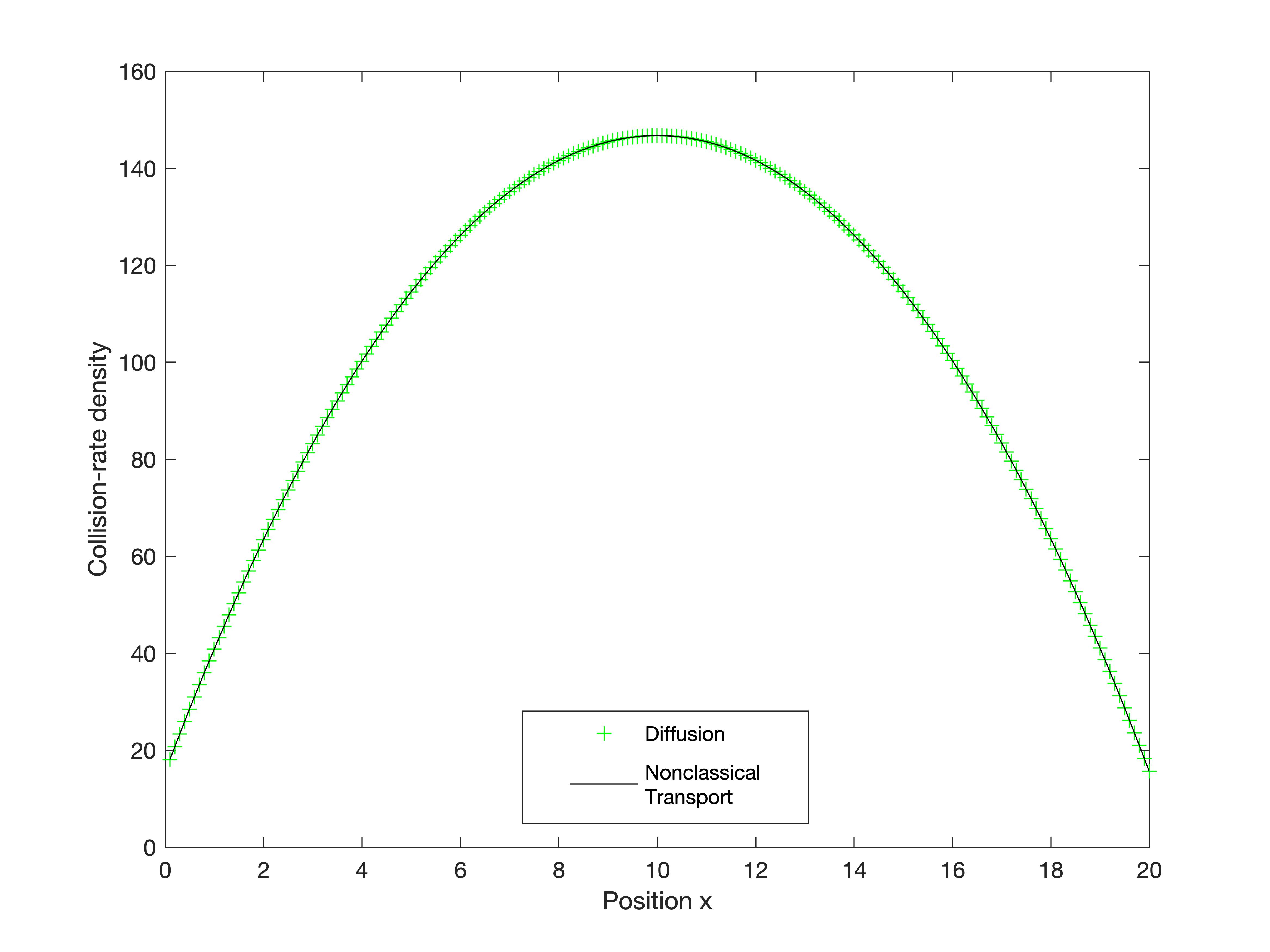
Figure 2: Collision-rate density generated with diffusion and nonclassical approaches

Table 2: Convergence Data for Nonclassical Transport with Nonexponential $p(s)$

	Number of		Spectral
	Iterations		Radius
$\mathbf{c}$	SI	S2SA	SI	S2SA
0.8	56	6	0.7997	0.1538
0.9	110	7	0.8997	0.1811
0.99	906	6	0.9989	0.1885
0.999	6443	6	0.9989	0.1802

At this point, we compare the iteration count and spectral radius for stand-alone source iteration (SI) and transport synthetic acceleration (S₂SA). We set $Q(x)=1.0$, and $p(s)$ and $\Sigma_{t}(s)$ are given respectively by Eqs. 4.6 and 4.8, with $\sigma_{t}=1.0$. Once more, we increase the domain size to $X=200$, and assume the truncation order of the Laguerre expansion to be $M=50$. Table 2 presents the number of iterations and the spectral radius for different choices of the scattering ratio $c$. Similar to the previous case, there is a reduction in both the spectral radius and iteration count, with a decrease of 3 orders of magnitude in the iterations for the highest scattering ratio.

5 Discussion

We have introduced a transport synthetic acceleration procedure that speeds up the source iteration scheme for the solution of the one-speed nonclassical spectral S_N equations in slab geometry. Specifically, we used S₂ synthetic acceleration to solve nonclassical spectral S₁₆ equations for problems involving exponential and nonexponential free-path distributions. The numerical results successfully confirm the advantage of the method; to our knowledge, this is the first time a numerical acceleration approach is used in this class of nonclassical spectral problems. Moreover, although we assumed for simplicity monoenergetic transport and isotropic scattering, extending the method to include energy-dependence and anisotropic scattering shall not lead to significant additional theoretical difficulties.

When compared to stand-alone SI, S₂SA yields a significant reduction in number of iterations (up to three orders of magnitude) and spectral radii. The values of the spectral radius for stand-alone SI remain virtually unchanged for the exponential and nonexponential cases for a fixed value of the scattering ratio $c$. However, all spectral radii for S₂SA are larger in the nonexponential case than in the exponential case for the same value of $c$, increasing from $6.5\%$ (when $c=0.999$) to $13.6\%$ (when $c=0.8$).

In fact, we do not see spectral radius values that are exactly consistent with those found when applying corresponding techniques to the classical S_N transport equation [37]. This can be attributed to the fact that the nonclassical equation contains an altogether different scattering term, which depends on the free-path $s$. Although a full convergence analysis is beyond the scope of this paper, we shall perform it in a future work in order to investigate this feature.

References

- [1] K. M. Case, P. F. Zweifel, Linear Transport Theory, Addison-Wesley, Reading, Massachusetts, 1967.
- [2] E. W. Larsen, A generalized Boltzmann equation for non-classical particle transport, in: Proceedings of the International Conference on Mathematics and Computation and Supercomputing in Nuclear Applications - M&C + SNA 2007, Monterey, CA, Apr. 15-19, 2007.
- [3] E. W. Larsen, R. Vasques, A generalized linear Boltzmann equation for non-classical particle transport, Journal of Quantitative Spectroscopy and Radiative Transfer 112 (4) (2011) 619 – 631.
- [4] M. Frank, T. Goudon, On a generalized Boltzmann equation for non-classical particle transport, Kinetic and Related Models 3 (3) (2010) 395 – 407.
- [5] R. Vasques, E. W. Larsen, Non-classical particle transport with angular-dependent path-length distributions. I: Theory, Annals of Nuclear Energy 70 (2014) 292 – 300.
- [6] E. d’Eon, Rigorous asymptotic and moment-preserving diffusion approximations for generalized linear Boltzmann transport in arbitrary dimension, Transport Theory and Statistical Physics 42 (6-7) (2014) 237 – 297.
- [7] M. Frank, K. Krycki, E. W. Larsen, R. Vasques, The nonclassical Boltzmann equation and diffusion-based approximations to the Boltzmann equation, SIAM Journal on Applied Mathematics 75 (3) (2015) 1329 – 1345.
- [8] R. Vasques, The nonclassical diffusion approximation to the nonclassical linear Boltzmann equation, Applied Mathematics Letters 53 (2016) 63 – 68.
- [9] M. Frank, W. Sun, Fractional diffusion limits of non-classical transport equations, Kinetic & Related Models 11 (2018) 1503 – 1526.
- [10] R. Vasques, R. N. Slaybaugh, Simplified PN equations for nonclassical transport with isotropic scattering, in: Proceedings of the International Conference on Mathematics and Computational Methods Applied to Nuclear Science and Engineering, Jeju, Korea, Apr. 16-20, 2017.
- [11] T. Camminady, M. Frank, E. W. Larsen, Nonclassical particle transport in heterogeneous materials, in: Proceedings of the International Conference on Mathematics and Computational Methods Applied to Nuclear Science and Engineering, Jeju, Korea, Apr. 16-20, 2017.
- [12] E. W. Larsen, M. Frank, T. Camminady, The equivalence of “forward” and “backward” nonclassical particle transport theories, in: Proceedings of the International Conference on Mathematics and Computational Methods Applied to Nuclear Science and Engineering, Jeju, Korea, Apr. 16-20, 2017.
- [13] I. Makine, R. Vasques, R. N. Slaybaugh, Exact transport representations of the classical and nonclassical simplified PN equations, Journal of Computational and Theoretical Transport 47 (4-6) (2018) 326 – 349.
- [14] E. d’Eon, A reciprocal formulation of nonexponential radiative transfer. 1: Sketch and motivation, Journal of Computational and Theoretical Transport 47 (2018) 84 – 115.
- [15] E. d’Eon, A reciprocal formulation of nonexponential radiative transfer. 2: Monte Carlo estimation and diffusion approximation, Journal of Computational and Theoretical Transport 48 (2019) 201 – 262.
- [16] A. B. Davis, A. Marshak, Solar radiation transport in the cloudy atmosphere: A 3D perspective on observations and climate impacts, Reports on Progress in Physics 73 (2) (2010) 026801.
- [17] K. Krycki, C. Berthon, M. Frank, R. Turpault, Asymptotic preserving numerical schemes for a non-classical radiation transport model for atmospheric clouds, Mathematical Methods in the Applied Sciences 36 (16) (2013) 2101 – 2116.
- [18] A. B. Davis, F. Xu, A generalized linear transport model for spatially correlated stochastic media, Journal of Computational and Theoretical Transport 43 (2014) 474 – 514.
- [19] F. Xu, A. B. Davis, D. J. Diner, Markov chain formalism for generalized radiative transfer in a plane-parallel medium, accounting for polarization, Journal of Quantitative Spectroscopy and Radiative Transfer 184 (2016) 14 – 26.
- [20] A. B. Davis, F. Xu, D. J. Diner, Generalized radiative transfer theory for scattering by particles in an absorbing gas: Addressing both spatial and spectral integration in multi-angle remote sensing of optically thin aerosol layers, Journal of Quantitative Spectroscopy and Radiative Transfer 205 (2018) 148 – 162.
- [21] A. B. Davis, F. Xu, D. J. Diner, Addendum to “Generalized radiative transfer theory for scattering by particles in an absorbing gas: Addressing both spatial and spectral integration in multi-angle remote sensing of optically thin aerosol layers”, Journal of Quantitative Spectroscopy and Radiative Transfer 206 (2018) 251 – 253.
- [22] R. Vasques, E. W. Larsen, Anisotropic diffusion in model 2-D pebble-bed reactor cores, in: Proceedings of the International Conference on Advances in Mathematics, Computational Methods, and Reactor Physics, Saratoga Springs, NY, May 3-7, 2009.
- [23] R. Vasques, Estimating anisotropic diffusion of neutrons near the boundary of a pebble bed random system, in: Proceedings of the International Conference on Mathematics and Computational Methods Applied to Nuclear Science & Engineering, Sun Valley, ID, May 5-9, 2013.
- [24] R. Vasques, E. W. Larsen, Non-classical particle transport with angular-dependent path-length distributions. II: Application to pebble bed reactor cores, Annals of Nuclear Energy 70 (2014) 301 – 311.
- [25] R. Vasques, R. N. Slaybaugh, K. Krycki, Nonclassical particle transport in the 1-D diffusive limit, Transactions of the American Nuclear Society 114 (2016) 361 – 364.
- [26] R. Vasques, K. Krycki, R. N. Slaybaugh, Nonclassical particle transport in one-dimensional random periodic media, Nuclear Science and Engineering 185 (1) (2017) 78 – 106.
- [27] M. Wrenninge, R. Villemin, C. Hery, Path traced subsurface scattering using anisotropic phase functions and non-exponential free flights, Tech. Rep. Technical Memo 17-07, Pixar Inc. (2017).
- [28] A. Jarabo, C. Aliaga, D. Gutierrez, A radiative transfer framework for spatially-correlated materials, ACM Transactions on Graphics 37 (4) (2018) 83:1–83:13.
- [29] B. Bitterli, S. Ravichandran, T. Müller, M. Wrenninge, J. Novák, S. Marschner, W. Jarosz, A radiative transfer framework for non-exponential media, in: SIGGRAPH Asia 2018 Technical Papers, New York, NY, Dec. 4-7, 2018.
- [30] J. Marklof, A. Strömbergsson, The distribution of free path lengths in the periodic Lorentz gas and related lattice point problems, Annals of Mathematics 172 (3) (2010) 1949 – 2033.
- [31] J. Marklof, A. Strömbergsson, The Boltzmann-Grad limit of the periodic Lorentz gas, Annals of Mathematics 174 (1) (2011) 225 – 298.
- [32] J. Marklof, A. Strömbergsson, Power-law distributions for the free path length in Lorentz gases, Journal of Statistical Physics 155 (6) (2014) 1072 – 1086.
- [33] J. Marklof, A. Strömbergsson, Generalized linear Boltzmann equations for particle transport in polycrystals, Applied Mathematics Research Express 2015 (2) (2015) 274 – 295.
- [34] F. Golse, Recent results on the periodic Lorentz gas, in: X. Cabré, J. Soler (Eds.), Nonlinear Partial Differential Equations, Springer Basel, 2012, pp. 39 – 99.
- [35] R. Vasques, L. R. Moraes, R. C. Barros, R. N. Slaybaugh, A spectral approach for solving the nonclassical transport equation, Journal of Computational Physics 402 (2020) 109078.
- [36] E. E. Lewis, W. F. Miller, Computational methods of neutron transport, American Nuclear Society, 1993.
- [37] M. L. Adams, E. W. Larsen, Fast iterative methods for discrete-ordinates particle transport calculations, Progress in Nuclear Energy 40 (1) (2002) 3 – 159.
- [38] U. W. Hochstrasser, Orthogonal polynomials, in: M. Abramowitz, I. A. Stegun (Eds.), Handbook of Mathematical Functions with Formulas, Graphs, and Mathematical Tables, Dover Publications, 2012, pp. 771 – 802.
- [39] R. Burden, J. Faires, Numerical Analysis, Dover, 1993.
- [40] M. L. Adams, Discontinuous finite element transport solutions in thick diffusive problems, Nuclear Science and Engineering 137 (3) (2001) 298–333.
- [41] G. I. Bell, S. Glasstone, Nuclear Reactor Theory, Van Nostrand Reinhold, New York, 1970.