Assessing the Early Bird Heuristic (for Predicting Project Quality)

Abstract.

Before researchers rush to reason across all available data or try complex methods, perhaps it is prudent to first check for simpler alternatives. Specifically, if the historical data has the most information in some small region, perhaps a model learned from that region would suffice for the rest of the project.

To support this claim, we offer a case study with 240 projects, where we find that the information in those projects “clumpe” towards the earliest parts of the project. A quality prediction model learned from just the first 150 commits works as well, or better than state-of-the-art alternatives. Using just this ”early bird” data, we can build models very quickly and very early in the project life cycle. Moreover, using this early bird method, we have shown that a simple model (with just a few features) generalizes to hundreds of projects.

Based on this experience, we doubt that prior work on generalizing quality models may have needlessly complicated an inherently simple process. Further, prior work that focused on later-life cycle data needs to be revisited since their conclusions were drawn from relatively uninformative regions.

Replication note: all our data and scripts are available here: https://github.com/snaraya7/early-bird

1. Introduction

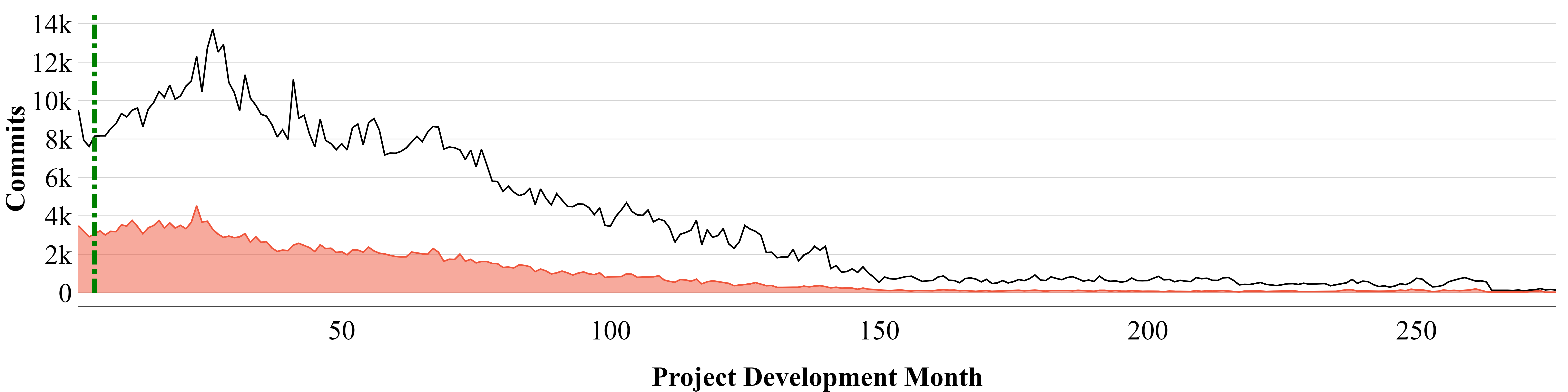
Figure 1.A: 155 popular GitHub projects (#stars$>1000$). Data from 1.2 million commits.

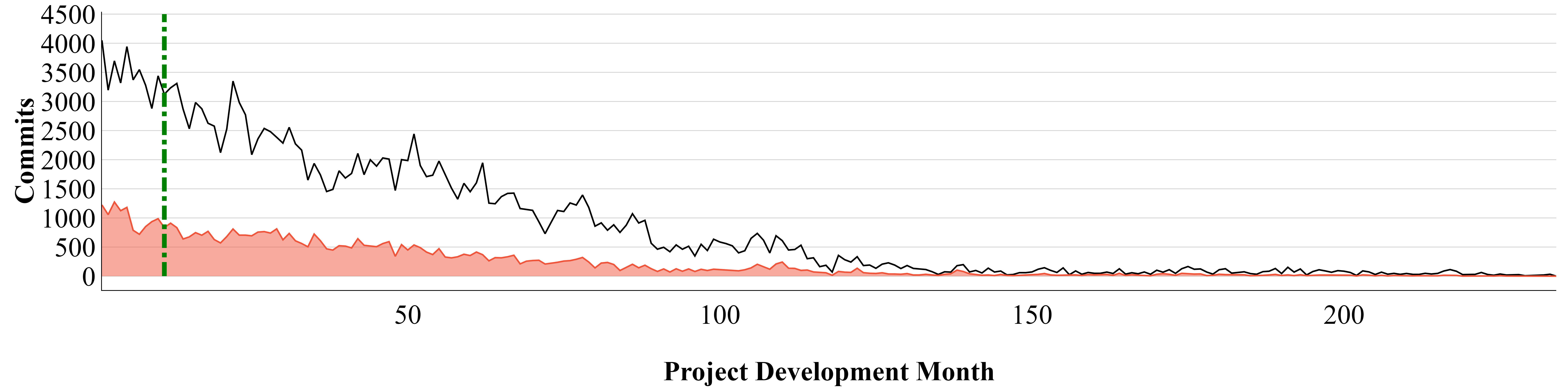
Figure 1.B: 85 unpopular GitHub projects (#stars$<1000$). Data from 253,289 commits.

Figure 1. Most defective commits occur early in the life cycle. Black:Red = Clean:Defective commits. In this paper, we compare (a) models learned up to the vertical green (dotted) line to (b) models learned using more data.

In software defect prediction, researchers often fail to try simpler methods before trying complex analytics (Shrikanth et al., 2021; Zhou et al., 2018). For example:

• “For many new projects we may not have enough historical data to train prediction models” (Rahman et al., 2012)

• “At least for defect prediction, it is no longer enough to just run a data miner and present the result without conducting a tuning optimization study.” (Fu et al., 2016)

• “Many research studies have shown that ensemble learning can achieve much better classification performance than a single classifier” (Yang et al., 2017)

While we do not doubt those results in that context, we show in this work that we can simplify software defect prediction if we focus more on the quality of the training data than on applying various software analytic techniques. Furthermore, this paper shows that many of the prevalent methods used to build defect predictors are needless and can be ‘simplified’ to a large extent with knowledge-rich early project data.

By simplified we mean:

• Stable conclusions (no need to update defect predictors for every new project release).

• Less run-time (With fewer project data we can find and build relevant predictors faster).

• Better explanations (With fewer features we can communicate the oracles (predictors) decisions to stakeholders effectively).

In our lab exercise, we have sometimes seen unsatisfactory results from such a complex approach. For example, once we tried learning defect attributes from 700,000+ commits. The web slurping required for that process took nearly 500 CPU days, using five machines with 16 cores, over seven days (since the data from those projects had to be cleaned, massaged, and transformed into some standard format). Within that data space, we found significant differences in the models learned from different parts of the data. So even after all that work and over a year of CPU, we were unable to report a stable conclusion to our business users.

This kind of experience motivate us to ask the question “when is enough data just enough to build effective defect predictors?” Our answer to this question comes from a previously unreported effect is shown in Figure 1. As shown in this figure, when we look at the percent of buggy commits in GitHub projects, a remarkable pattern emerges. Specifically, most of the buggy commits occur earlier in the life cycle.

This observation prompted an investigation of the “early bird” heuristic (or the “early-data-lite” sampling method) that just uses early life cycle data to predict defects. The literature review of §4 shows that, surprisingly, this approach to software defect prediction has been overlooked by prior work (Shrikanth et al., 2021). This is a significant oversight since, in 240 GitHub projects, we can show that defect predictors learned from the first 150 commits work as well, or better, than state-of-the-art alternatives.

Our prior work showed early-data-lite ($E$) within project supervised defect prediction models performed statistically better or on par with those that were built using either recent ($RR$) or abundant commits ($ALL$) (Shrikanth et al., 2021). In this work, we exploit the early-data-lite ($E$) method to answer four research questions (RQs), they are:

• RQ1: Can we build early software defect prediction models from unpopular projects?

• RQ2: Can we build early software defect prediction models with fewer features?

• RQ3: Can we build early software defect prediction models by transferring early life cycle data from other projects?

• RQ4: Do complex methods supersede early software defect prediction models?

Results of four RQs in §6 confirm that the software defect prediction model built from another project (cross) from the same organization using the early bird heuristic can identify defects in local projects having fewer commits. Notably, the early bird (discussed later in §2.2) heuristic offers the following benefits: a) only the first 150 commits are considered for training; therefore the cross-project can be young (only a few months old), b) we find using only two size-based features to build defect prediction models was sufficient, c) the cross-project need not be well maintained (unpopular) and d) the results also indicate that much of the augmenting machine learning practices such as hyper-parameter optimization and ensemble learning were needless.

Overall, the contributions of this paper are to show:

• The information (like software defects) within projects may not be evenly distributed across the life cycle. For such data, it can be very useful to adopt a “early-data-lite” approach.

• For example, early life cycle data finds simple models (with only two features) that generalize across hundreds of projects. Such models can be built much faster than traditional methods (weeks versus months of CPU time).

• So before researchers use all available data, they need to first check that their buggy commit data occur at equal frequency across the life cycle. We say this since much prior work on methods for learning from multiple projects (Menzies et al., 2011; Li et al., 2012; Ma et al., 2012; He et al., 2012; Menzies et al., 2012; Bettenburg et al., 2012; Rahman et al., 2012; Turhan et al., 2013; Nam et al., 2013a; Peters et al., 2013a; Canfora et al., 2013; Peters et al., 2013b; Herbold, 2013; He et al., 2013; Rahman and Devanbu, 2013; Fukushima et al., 2014; Panichella et al., 2014; Zhang et al., 2014; Ryu et al., 2015; Chen et al., 2015; Zhang et al., 2015; Peters et al., 2015; Canfora et al., 2015; Jing et al., 2015; He et al., 2015; Zhang et al., 2016c; Kamei et al., 2016; Yang et al., 2016; Ryu et al., 2016; Xia et al., 2016a; Jing et al., 2016; Ryu and Baik, 2016; Zhang et al., 2016b; Krishna et al., 2016; Wang et al., 2016a; Ryu et al., 2017; Nam et al., 2017; Ni et al., 2017; Zhou et al., 2018; Chen et al., 2018b; Hosseini et al., 2018; Krishna and Menzies, 2018; Li et al., 2018; Wang et al., 2018; Wu et al., 2018; Dam et al., 2018; Huang et al., 2019; Chen et al., 2019a, b; Liu et al., 2019) needlessly complicated an inherently simple process.

Table 1. Table of Important Acronyms

Acronym	Abbreviation
AUC	Area under the receiver operating characteristic curve
CFS	Correlation-based Feature Selection
DODGE	Optimizer proposed by Agrawal et al. in (Agrawal et al., 2019)
DT	Decision Tree
HPO	Hyperparameter optimization
HYPEROPT	Optimizer proposed by Bergstra et al. (Bergstra et al., 2011)
IFA	Initial Number of False Alarms
KNN	k-nearest neighbors algorithm
LA and LT	Refer to features list in Table 4
LR	Logistic Regression
MCC	Matthews correlation coefficient
NB	Naive Bayes classifier
PF	False Alarm Rate
RF	Random forest
SMOTE	Synthetic Minority Over-sampling Technique (Chawla et al., 2002)
SVM	Support vector machines
SZZ	Sliwerski Zimmerman Zellar Algorithm (Śliwerski et al., 2005)
TCA	Transfer Component Analysis (Nam et al., 2013a)
TLEL	Two-layer Ensemble Learning Algorithm (Yang et al., 2017)
TPE	Tree-structured Parzen Estimator (Bergstra et al., 2011)

The rest of this paper explains our method; and offers experimental evidence that this early-bird method works better than sophisticated methods like classifier tuning, ensemble and notably made transfer learning algorithms work simpler, faster, and more stable. This paper uses the abbreviations of Table 1.

Before all that, we digress to address the obvious objections to our conclusion. The results presented here are only for software defect prediction. In future work, we need to test if our results hold for other domains.

2. Connection to Prior Work

2.1. Initial Report

Previously, we have reported the Figure 1. A results at ICSE’21 (Shrikanth et al., 2021). We calculate that only Figure 1.A and 5 pages of this text (e.g. §8.1) come from that prior work.

As to the semantic difference between this paper to prior work, that prior study was more limited since it did not have the additional data of Figure 1.B. Also, that prior study only ran some within-project sampling methods on the Figure 1.A data. This paper takes the additional step of comparing our methods to transfer learning, classifier tuning, and ensemble methods. Further, previously, we did not report the model learned via this method. We show here that a simple model (that uses just a few variables) can be learned from a few early life cycle samples. Lastly, as shown by the new results of this paper in Table 7, Table 8, Table 9, and Table 10 we can out-perform that results from that prior work. Hence, it is important to ingest the results of our prior work first, especially to understand why we omit certain treatments in our experiments in this work.

2.2. Early Bird Heuristic

In our prior work, we find that much of the software engineering (SE) project activity occurs during the early periods of the software project life-cycle (Shrikanth et al., 2021). We used that observation as a heuristic to answer if defect prediction models can stop learning early. Interestingly, we found that defect prediction models that learned from just 150 commits (which occurred in less than four months of the project) yield statistically the same predictive performance as models trained with recent or all available project data (commits) . In this work, we label this effect as the ‘early-bird’ heuristic (or $E$).

Software defect predictors built in the literature or practice using all available data are data-hungry or those that use recent project data may be labeled as late data. The defect prediction models built using the ‘early-bird’ heuristic are early-data-lite as they use only a tiny portion (4%) of the early project data (Shrikanth et al., 2021). Data-hungry models are frequently re-trained and this gives rise to the conclusion-instability issue (Krishna and Menzies, 2018). In other words, retraining would cause the models to behave differently for every project release (e.g, A commit classified as defective in release ‘X’ may be classified as clean in release ‘X+1’). Early-data-lite models are ‘never retrained’ as they always use the fixed 150 early project commits to building defect predictors.

3. Motivation

3.1. Defect Prediction

The case studies of this paper are based on software defect prediction. Hence, before doing anything else, we need to introduce that research area.

Fixing software defects is not cheap (Hailpern and Santhanam, 2002). Accordingly, for decades, SE researchers have been devising numerous ways to predict software quality before deployment. One of the oldest studies was made in 1971 by Akiyama using size-based defect predictions for a system developed at Fujitsu, Japan (Akiyama, 1971). This approach remains popular today. A 2018 survey of 395 practitioners from 33 countries and five continents [20] found that over 90% of the respondents were willing to adopt software defect prediction techniques (Wan et al., 2018).

Software defect prediction uses data miners to input static code attributes and output models that predict where the code probably contains most bugs (Ostrand et al., 2005; Menzies et al., 2006). The models learned in this way are very effective and relatively cheap to build:

• Effective: Misirili et al.  (Misirli et al., 2011), and Kim et al. (Kim et al., 2011) report considerable cost savings when such predictors are used in guiding industrial quality assurance processes.

• Relatively simpler to implement Also, Rahman et al. (Rahman et al., 2014) show that such predictors are competitive with more elaborate approaches. For example, they note that static code analysis tools can have expensive licenses that need to be updated after any major language upgrade. Defect predictors, on the other hand, can be quickly implemented via some lightweight parsing of commit-level metrics that are programming language agnostic.

Our prior work (Shrikanth et al., 2021) proposed numerous extensions that improve the validity and scope of the “early-data-lite” method. Therefore, in this work we continue to assess the efficacy and applicability of the “early-data-lite” method broadly on two active areas in software defect prediction, specifically:

• Data: Transfer Learning (Cross-project defect prediction)

• Technique: Tuning and Ensemble methods

3.2. Data: Transfer Learning

Defect predictors are learned from project data. What happens if there is not enough data to learn those models? This is an especially acute problem for newer projects (and in the absence of historical data in some legacy projects (Briand et al., 2002)).

In such scenarios, practitioners and researchers might identify matured projects that share some similarities to their local projects. Once found, then lessons learned could be transferred from the older to the new project. There are kinds of transfer:

• Cross: cross-project defect prediction. Lessons learned from other projects and applied to this project.

• Within: within-project defect prediction. Using data from this project, lessons learned from prior experience are used to make predictions about later life cycle development.

To say the least, transfer learning is a very active research area in SE. We can find more than 1,000 articles in the last five years alone (found using the query ”cross-project defect prediction,” ). By our count, within that corpus, there have been at least two dozen transfer learning methods  (Amasaki, 2020). Interesting methods evolved in that research include:

• Heterogeneous transfer that lets data expressed indifferent formats transferred from project to projects (Nam et al., 2017);

• Temporal transfer learning, which is a within-project defect prediction (Within) tool where earlier life cycle data is used to make predictions later in the life cycle (Kocaguneli et al., 2015).

Our reading of the literature is that, apart from our own research, the prior state-of-the-art in the SE literature is Nam et al.’s $TCA+$ (Transfer Component Analysis) method (Nam et al., 2013a). For a list of important abbreviations used in this paper see Table 1. Given data from a source and a target project, TCA strives to “align” the source and target data via dimensionality rotation, expansion, and contraction. TCA+ is an extension to basic TCA that used automatic methods to find normalization options for TCA.

3.3. Technique : Tuning and Ensemble

Classification algorithms can be trained to classify a project commit as defective. Studies have shown their predictive performance can depend upon the set of hyper-parameter they are initially configured (Fu et al., 2016; Agrawal et al., 2019).

For example, the k-nearest neighbors ($KNN$) that we explore in this study are available in the widely used scikit-learn (Pedregosa et al., 2011b) machine learning library. And $KNN$ is set to the following default parameters based on standard machine learning literature as follows:

$n\_{\mathit{n}eighbors}=5,*,{\mathit{w}eights}={\mathit{u}niform},{\mathit{a}lgorithm}={\mathit{a}uto},{\mathit{l}eaf}\_{\mathit{s}ize}=30$,

$p=2,{\mathit{m}etric}={\mathit{m}inkowski},{\mathit{m}etric}\_{\mathit{p}arams}={\mathit{N}one},n\_{\mathit{j}obs}={\mathit{N}one}$

However, as seen from the numerous parameters available for $KNN$, there is a huge parameter space of options the $KNN$ can be tried and tested (tuned). Therefore most machine learning algorithms’ hyper-parameters can be tuned using training data before being tested on project releases in our case.

There are numerous ways to find the right set of parameters for a classifier given the training data. But the decision predominantly comes with the run-time cost. For example, searching through all available options ‘Manual Search’ may not terminate. One may try ‘Random Search’ with a terminating condition but the probability of finding the near-best parameter may be low. Fu et al. (Fu et al., 2016) explored ‘grid-search’ a baseline hyper-parameter approach in the field of machine learning (Fu et al., 2016) but found it to be very slow for software defect prediction. Recently (2019) Agrawal et al. proposed a novel optimizer that terminates quickly after finding near-optimal hyper-parameters for defect predictors (Agrawal et al., 2019). More details on DODGE will be presented in §5.3.1. Therefore this paper will explore DODGE with early methods.

Another avenue of complex approach is the use of the ensemble method, where the philosophy is why use just ‘one’ when ‘more’ is better. Numerous studies have shown defect predictors can be improved significantly when an ensemble of classifiers were used rather than just one (Yang et al., 2017; Wang and Yao, 2013; He and Garcia, 2009). In 2017, Yang et al. proposed a two-layer ensemble approach for software defect prediction called TLEL (Two-layer Ensemble Learner) that showed promising improvements when compared to predictors with a single classifier. §5.3.3 elucidates its operation and this paper will explore TLEL as part of the complex methods to test the efficacy of early methods.

3.4. Issues with current approaches

Nevertheless, just because a technique is popular does not mean that it should be recommended. Our reading of the literature is most recent SE analytics papers have taken a complex approach (e.g. see the quotes in our prior work (Shrikanth et al., 2021)) and use state-of-the-art analytics without testing with simpler alternatives (Zhou et al., 2018). We argue there that it can be useful to try early-data-lite before adopting complex techniques that demand more data, delay analytics, do not offer explanations, and overutilize system resources. Because, for one thing, all that data might not be available. The availability of more data in an industrial setting is not assured. Further, it may not be useful to learn from more data. Proprietary data may not be readily available for practitioners to build predictors for their local projects. Zimmermann et al. showed that transferring predictors from the same domain does not guarantee quality predictions (Zimmermann et al., 2009). Finally, due to privacy concerns, teams even within the same organization may not readily make their matured project available for others to use (Peters et al., 2013b).

Another thing, several researchers have reported that a complex approach can be problematic:

• In our introduction, we reported on our own issues seen when learning from 700,000+ GitHub commits.

• At her ESEM’11 keynote address, Elaine Weyuker questioned whether she will ever have the option to make the AT&T information public (Weyuker et al., 2008).

• In over 30 years of COCOMO effort, Boehm could share cost estimation data from only 200 projects (Boehm et al., 2005).

Next, applying techniques discussed in §5.8 comes with a CPU run-time cost. When time to time researchers have strived and endorsed to look for simpler alternatives it is important that we explore them.

4. Related Work

In our prior work , we showed that historical data within the project were used in large quantities to build defect predictors that were needless (Shrikanth et al., 2021). And as promised in our prior work in this work we check the validity of our prior conclusion beyond within-project software defect prediction and test the efficacy of early methods in various contexts such as:

• Unpopular SE projects

• Transfer learning scenarios

• Hyper-parameter optimization and Ensemble approach

One reason to explore early life cycle data reasoning is that it has not been done before (except our prior work that focuses on within-project data to build predictors). Fenton et al. (2008) examined the use of human judgment rather than domain data to handcraft a causal model to predict residual defects (defects discovered during operational usage or independent testing), however, this required extensive work (2 years) and we do not explore this path (Fenton et al., 2008). Zhang and Wu demonstrated in 2010 that fewer programs sampled from an entire space of programs (covering the entire project life-cycle) can be used to estimate project quality (Zhang and Wu, 2010). The difference here is that we sample them ‘early’ in the project life-cycle and not the entire project history. Rahman et al. endorse employing a substantial sample size in defect prediction models to reduce bias (Rahman et al., 2013). While we do not deny bias in defect prediction data sets, we find that the performance of our proposed early data-lite approach is comparable to that of prior approaches. Arokiam and Jeremy looked into bug severity prediction (Arokiam and Bradbury, 2020). They demonstrate that data transferred from other projects can be used to predict bug severity early in project development. Similar to Arokiam and Jeremy’s work, Sousuke examined Cross-Version defect prediction (CVDP) using Cross-Project Defect Prediction (CPDP) data in 2020 in  (Amasaki, 2020). Their study with 41 releases suggests that the most recent project release was still superior to the majority of CPDP approaches. However, in contrast to Sousuke, we provide contrary evidence in this work. Notably, we evaluate our strategy using more than a thousand releases and seven performance metrics.

We expanded the scope of early life cycle data reasoning in the subsequent §4.1 through a literature survey on other prominent defect prediction approaches specifically transfer learning, hyper-parameter optimization, and ensemble approach. Notably, these methods demand more data and computing resources making it difficult to predict defects early in the project life cycle.

We find that much of the SE transfer learning methods (Turhan et al., 2013; Nam et al., 2013a; Peters et al., 2013a; Canfora et al., 2013; Peters et al., 2013b; Fukushima et al., 2014; Panichella et al., 2014; Ryu et al., 2015; Chen et al., 2015; Zhang et al., 2015; Peters et al., 2015; Canfora et al., 2015; Jing et al., 2015; Kamei et al., 2016; Yang et al., 2016; Ryu et al., 2016; Xia et al., 2016a; Jing et al., 2016; Ryu and Baik, 2016; Zhang et al., 2016b; Krishna et al., 2016; Ryu et al., 2017; Nam et al., 2017; Ni et al., 2017; Zhou et al., 2018; Chen et al., 2018b; Hosseini et al., 2018; Krishna and Menzies, 2018; Li et al., 2018; Wang et al., 2018; Huang et al., 2019) and Tuning or ensemble methods  (Bowes et al., 2018; Tan et al., 2015; Xia et al., 2016a; Laradji et al., 2015; Tantithamthavorn et al., 2016; Wang et al., 2018; Ryu et al., 2016; Zhou et al., 2019; Tantithamthavorn et al., 2018; Rhmann et al., 2020; Kamei et al., 2016; Yang et al., 2017; Chekam et al., 2020; Song et al., 2018; Bird et al., 2011; Ghotra et al., 2015; Wang and Yao, 2013; Ryu et al., 2015; Panichella et al., 2014; Jing et al., 2016; Ryu et al., 2017; Peters et al., 2013a; Wang et al., 2016b; Sun et al., 2012; Siers and Islam, 2015; Pandey et al., 2020; Huda et al., 2018; Xu et al., 2019; Tong et al., 2018; Pascarella et al., 2019; Rathore and Kumar, 2017; Kamei et al., 2016; Lam et al., 2017; Ye et al., 2014; Scandariato et al., 2014; Agrawal and Menzies, 2018; Agrawal et al., 2018; Zhang et al., 2016b; Agrawal et al., 2019; Jiang et al., 2013; Fu et al., 2016; Li et al., 2017; Wang et al., 2016a; Liu et al., 2019) could be characterized as “late-data” (or data-hungry) since they transferred all available data from one or more projects to build their predictors supporting our claim that this space has not been explored before.

As to other comparison studies, we explore transfer learning and hyper-parameter optimization in this paper. Prior to this paper, we focused extensively on transfer learning and hyper-parameter optimization at prominent venues (Krishna and Menzies, 2018; Krishna et al., 2016; Agrawal et al., 2019; Agrawal et al., 2021) because we believed those were “state-of-the-art” (and had convinced many journal reviewers of that proposition). After this paper, our views have changed and like many other researchers, we believe we have needless elaborated an inherently very simple process.

4.1. Literature Survey

Table 2. 50 ‘highly cited’ (more than 10 citations per year) papers that ran one or more Cross experiment(s) since 2011.

Year	#Data	#Features	Projects	Cites/Year	Paper
2011		20	2	16.44	(Menzies et al., 2011)
		198	6	19.25	(Li et al., 2012)
		17	10	39.13	(Ma et al., 2012)
		20	10	30.13	(He et al., 2012)
		20	7	23.38	(Menzies et al., 2012)
		20	2	13.88	(Bettenburg et al., 2012)
2012		8	9	25.38	(Rahman et al., 2012)
		16	41	14	(Turhan et al., 2013)
		17	8	48.43	(Nam et al., 2013a)
		20	41	22.43	(Peters et al., 2013a)
		20	10	19.57	(Canfora et al., 2013)
		20	10	13.29	(Peters et al., 2013b)
		20	14	13.29	(Herbold, 2013)
		20	10	11.43	(He et al., 2013)
2013		54	12	32	(Rahman and Devanbu, 2013)
		14	11	16.5	(Fukushima et al., 2014)
		20	10	20.5	(Panichella et al., 2014)
2014		26	1398	18.5	(Zhang et al., 2014)
		18	7	13.4	(Ryu et al., 2015)
		20	11	19.8	(Chen et al., 2015)
		20	10	14.4	(Zhang et al., 2015)
		20	17	12.4	(Peters et al., 2015)
		20	10	11.2	(Canfora et al., 2015)
		28	11	24.4	(Jing et al., 2015)
2015		20	10	33	(He et al., 2015)
	None	X	26	35.5	(Zhang et al., 2016c)
		14	11	26.5	(Kamei et al., 2016)
		14	6	19.75	(Yang et al., 2016)
		17	10	23.5	(Ryu et al., 2016)
		20	10	35.5	(Xia et al., 2016a)
		20	21	20.75	(Jing et al., 2016)
		20	30	11.75	(Ryu and Baik, 2016)
		26	1390	16.25	(Zhang et al., 2016b)
		61	23	10.5	(Krishna et al., 2016)
2016		X	10	70.25	(Wang et al., 2016a)
		20	15	21.33	(Ryu et al., 2017)
		61	34	80	(Nam et al., 2017)
2017		61	8	10.67	(Ni et al., 2017)
		6	58	21.5	(Zhou et al., 2018)
		14	6	20.5	(Chen et al., 2018b)
		20	11	23	(Hosseini et al., 2018)
		61	18	18.5	(Krishna and Menzies, 2018)
		61	28	14.5	(Li et al., 2018)
		20	10	14	(Wang et al., 2018)
		61	16	19.5	(Wu et al., 2018)
2018		X	10	20	(Dam et al., 2018)
		14	6	17	(Huang et al., 2019)
		61	8	14	(Chen et al., 2019a)
		20	7	20	(Chen et al., 2019b)
2019		20	14	19	(Liu et al., 2019)

KEY:   Part, All, None - No training data,
X - Features automated

Table 3. 44 ‘highly cited’ (more than 10 citations per year) papers that built software defect prediction models applying methods based on ensemble/tuning/both in the past decade (2011 to 2020).

Year	Cites/Year	Type	#Data	Projects	Paper	Year	Cites/Year	Type	#Data	Projects	Paper
2011	37.9		All	2	(Bird et al., 2011)	2013	25		All	6	(Jiang et al., 2013)
2012	17.33		All	14	(Sun et al., 2012)	2014	33		All	6	(Ye et al., 2014)
2013	54.13		All	10	(Wang and Yao, 2013)	2014	36.86		All	20	(Scandariato et al., 2014)
2013	24		All	41	(Peters et al., 2013a)	2016	15.8		All	1,390	(Zhang et al., 2016b)
2014	22		All	10	(Panichella et al., 2014)	2016	33.4		Part	17	(Fu et al., 2016)
2015	53.33		All	29	(Ghotra et al., 2015)	2016	79.8		Part	10	(Wang et al., 2016a)
2015	13.33		All	7	(Ryu et al., 2015)	2017	29.25		All	6	(Lam et al., 2017)
2015	18.17		All	6	(Siers and Islam, 2015)	2017	47.25		Part	7	(Li et al., 2017)
2016	29.2		All	11	(Kamei et al., 2016)	2018	37		All	9	(Agrawal and Menzies, 2018)
2016	22.4		All	21	(Jing et al., 2016)	2018	44		All	8	(Agrawal et al., 2018)
2016	15.8		All	12	(Wang et al., 2016b)	2019	14		All	10	(Agrawal et al., 2019)
2017	31		All	6	(Yang et al., 2017)	2019	18.5		Part	14	(Liu et al., 2019)
2017	22.5		All	15	(Ryu et al., 2017)	2020	28	TUNING	All	32	(Kamei et al., 2016)
2017	16.25		Part	11	(Rathore and Kumar, 2017)	2015	32.67		All	7	(Tan et al., 2015)
2018	32.67		All	27	(Song et al., 2018)	2015	44		All	6	(Laradji et al., 2015)
2018	21.33		All	15	(Huda et al., 2018)	2016	37.2		All	10	(Xia et al., 2016a)
2018	27.67		All	12	(Tong et al., 2018)	2016	50.8		All	18	(Tantithamthavorn et al., 2016)
2019	26		All	44	(Xu et al., 2019)	2016	24.4		All	10	(Ryu et al., 2016)
2019	21.5		Part	10	(Pascarella et al., 2019)	2018	31		All	18	(Bowes et al., 2018)
2020	28		All	2	(Rhmann et al., 2020)	2018	19.67		All	6	(Wang et al., 2018)
2020	31		All	3	(Chekam et al., 2020)	2018	47.67		Part	18	(Tantithamthavorn et al., 2018)
2020	20	ENSEMBLE	All	12	(Pandey et al., 2020)	2019	13.5	BOTH	All	25	(Zhou et al., 2019)

KEY:   Part, All

To understand more about late-data (data-hungry) reasoning in SE, we queried Google Scholar  to find software defect prediction articles (similar to our prior work (Shrikanth et al., 2021)) in three areas:

• We found 982 articles in Google Scholar using the query (“cross-project defect prediction”) in the last ten years.

• We found more than 1,740 articles in the last five years alone (searching the query “defect prediction” AND “(tuning OR hyper-parameter optimization) and 3,050 articles using the query “defect prediction” AND “ensemble”.

Following the advice of Agrawal et al. (Agrawal and Menzies, 2018), and Mathews et al. (Mathew et al., 2018) we focused only on “highly cited” papers, i.e., those with more than ten citations per year. Reading those papers, and after discarding papers pure of survey nature, we filtered the papers that performed some transfer learning experiments or a complex method ( ensemble or tuning). We summarized the results of this literature survey in Table 2 (Transfer learning) and Table 3 (Tuning and Ensemble methods).

Within those three sets, we found three approaches to row selection:

• ‘All’ if the methods of that paper used all rows (training data instances) from one or more projects to build defect predictors.

• ‘Part’ if the methods of that paper explore a large search space of one or more projects to find a small set of rows that are worthy of transfer data.

• In one case, in 2016, we also found a ‘None’ approach that used no training but just clustered the test data to find outliers, which were then labeled as bugs (Zhang et al., 2016c). Having recorded that method, this paper will not explore this minority approach.

Note that regardless of being “All” or “Part”, the analysis looks at the data across the entire life cycle before returning some or all of it.

As to other kinds of data selection, for all these papers, we counted:

• The number of projects used in those studies;

• The number of features used by their predictors.

• The applied any ensemble or tuning or both techniques.

When we tried to place this paper into Table 2 and Table 3, we found that our approach was, quite literally, off the charts. The methods advocated by this paper are neither “whole” nor “part” since we learn from early data, then stop collecting (so unlike all the research in Table 2 and Table 3, we never look at all the data). Further, our “number of projects”=1 (which does not even appear in Table 2) and we only use a handful of features (far fewer than the features used by other work in Table 2).

Hence we assert, with some confidence, that the methods of this paper have not been previously explored.

4.1.1. Representative Techniques

In order to design an appropriate experiment, we used the following guidelines.

Firstly, we are comparing the early sample to sampling over a larger space of project data. Hence, in the following, we will show early versus all experiments.

Secondly, there are two ways to find data: within-project and cross-project. Therefore, we will divide the early early-data and all late-data experiments into:

• early-data: early-within and early-cross

• late-data: all-within and all-cross

• Complex Methods: Optimizers (DODGE and HyperOpt) and ensemble method (TLEL).

Lastly, looking into the literature, we can see some clear state-of-the-art algorithms that should be represented in our study (specifically, the $TCA+$ and $Bellwether$ cross-project learning methods (Krishna et al., 2016; Nam et al., 2013a)). Accordingly, when exploring cross-project learning, we will employ those methods.

Explaining the exact methods used in this study requires some further details on those algorithms. Please see §5.2 for the algorithm details and for a discussion of what algorithms we selected. But, in summary, to the best of our knowledge, the early-data variants of these techniques have not been explored before in SE.

Table 4. 14 Commit level features that Commit Guru tool (Kamei et al., 2012; Rosen et al., 2015) mines from GitHub repositories

Dimension	Feature	Definition
	NS	Number of modified subsystems (subsystem identified using root directory (package) name)
	ND	Number of modified directories
	NF	Number of modified files
Diffusion	ENTROPY	Distribution of modified code across each file
	LA	Lines of code added
	LD	Lines of code deleted
Size	LT	Lines of code in a file before the change
Purpose	FIX	Whether or not this change is a defect fixing change.
	NDEV	#developers changing modified files
	AGE	Mean time from last to the current change
History	NUC	#changes to modified files before
	EXP	Developer experience
	REXP	Recent developer experience
Experience	SEXP	Developer experience on a subsystem

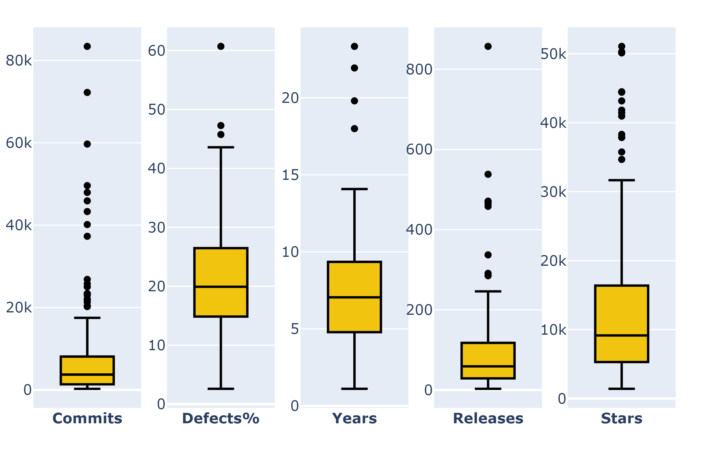
((a)) Popular projects (stars $\mathit{>1000}$).
Distributions seen in all 1.2 millions of commits of all
155 popular projects: median values of commits
(3,728), percent of defective commits (20%), life
span in years (7), releases (59) and stars (9,149).

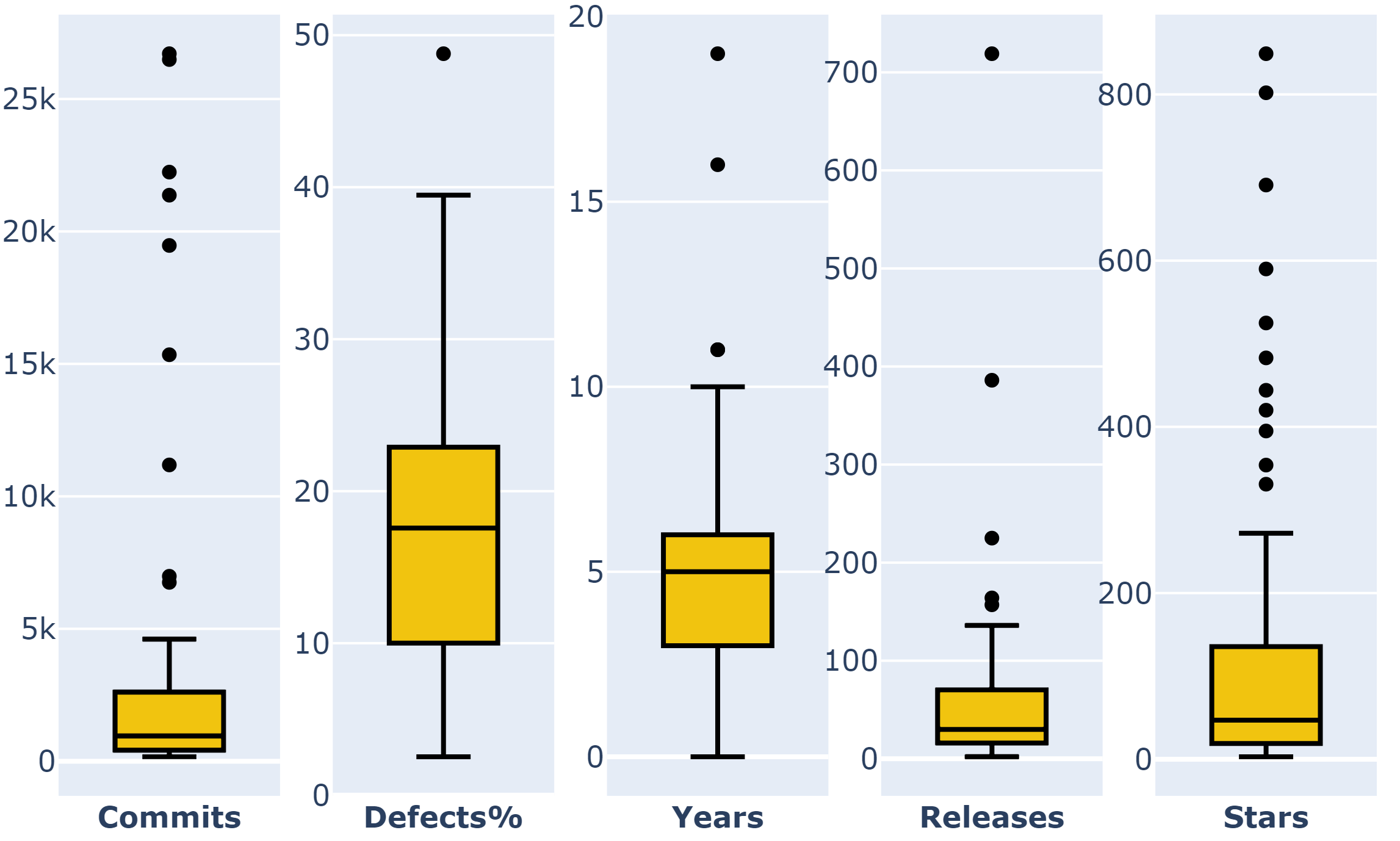
((b)) Unpopular projects (stars $\mathit{<1000}$).
Distributions seen in all 258,000+ commits of all 89 unpopular projects: median values of commits (957), percent of defective commits (18%), life span in years (5), releases (30) and stars (47).

Figure 2. 240 GitHub project data distributions.

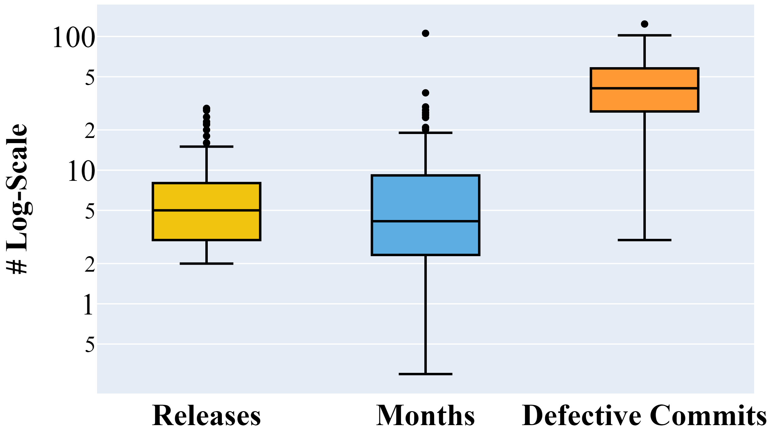
((a)) Popular projects. Median= 5 releases, 4 months, and 41 defective commits.

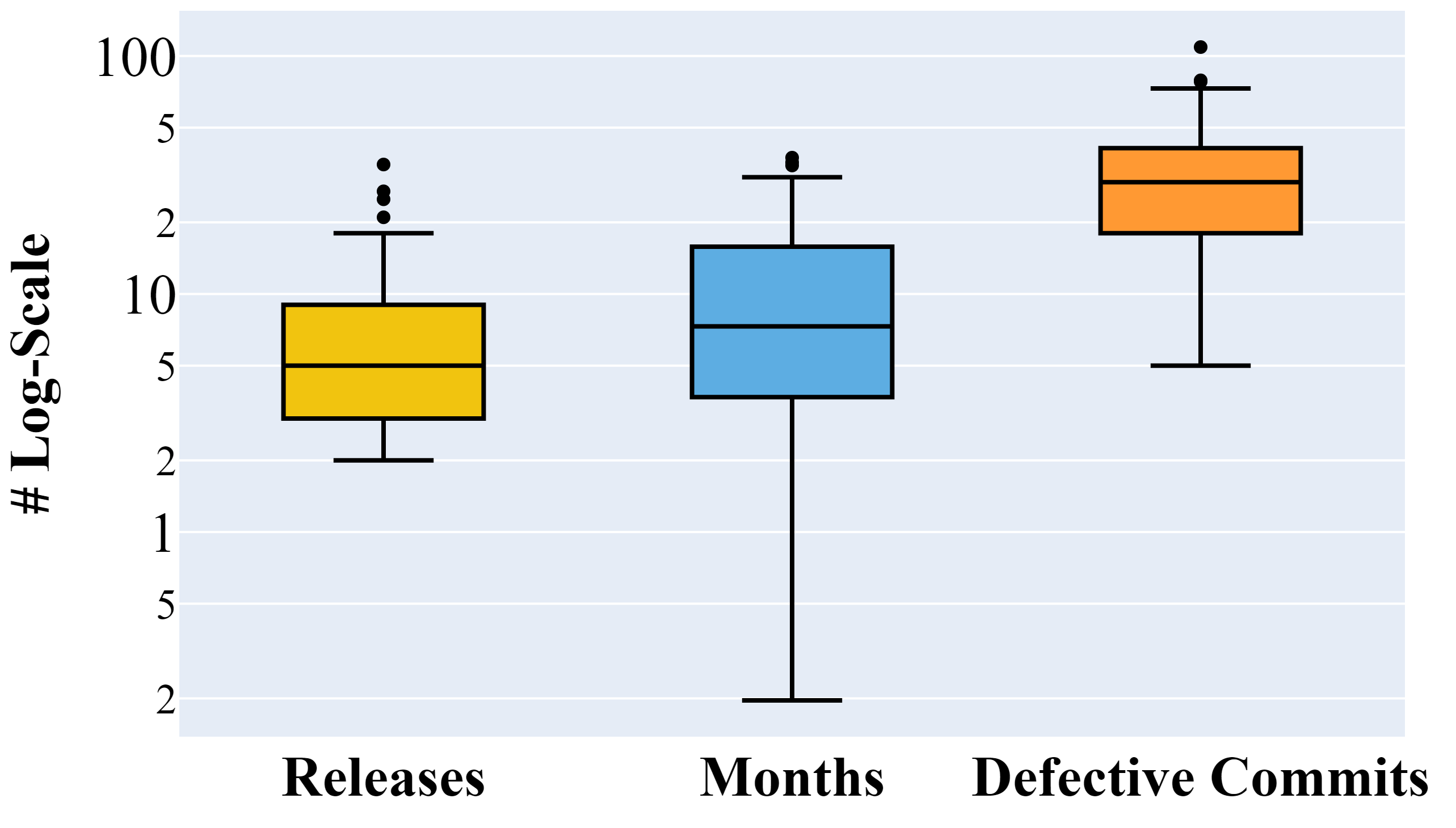
((b)) Unpopular projects. Median= 5 releases, 7 months, and 29 defective commits.

Figure 3. Distributions seen in the first 150 commits.

We understand the above areas do not cover all of the software defect prediction literature but to the best of our knowledge, we assert that we covered a range of active research areas within defect prediction to test the scope of our conclusion about early methods.

5. Experimental Methods

The rest of this paper assesses supervised defect prediction models built using the early-bird heuristic versus other learning policies and optimization techniques for the data of Figure 1.

At a high level, we build a defect prediction model in three steps.

First, we sample training commits using one of the sampling methods listed in §5.8. The test data is the commits from a project release. In the case of within-project defect prediction, past commits are never used as test commits. In all the experiments of this paper, there is no overlap of commit data between test and training data. Second, training and test commits are pre-processed using the techniques listed in §5.7. Third, we build the model using one of the classifiers listed in §5.2.

We use the measures listed in §5.9 to assess the performance of the defect prediction model’s ability to classify test commits (as defective or clean). This process of training, testing, and evaluation is repeated for every applicable project release in all 240 projects. Apart from RQ1, all other RQs consider all 240 GitHub projects for analysis.

Lastly, to compare the overall performance of various treatments we apply the Scott-Knott test discussed in §5.10. Here treatment is a defect prediction model built using a specific ‘sampling method’, ‘classifier’ and evaluated on a particular ‘measure.’ For example, one treatment can be a logistic regression-based defect prediction model that uses an early-bird (early-data) sampling method. Another could be a decision-tree-based model that used a data-hungry (late-data) sampling method. The population in this example is the distribution of ‘Recall’ scores evaluated in all the applicable project releases. The two treatments are then ranked (clustered) using the Scott-Knott test on the basis of an evaluation measure (say ‘Recall’).

5.1. Data

All data used in this study comes from open-source projects hosted on GitHub that other SE researchers can replicate. For details on that data, see Table 4, Figure 2 and Figure 3.

We reuse the 155 popular projects from our prior study which was randomly sampled from the project list curated by Munaiah et al. (Munaiah et al., 2017). Additionally, we collected 85 unpopular projects to answer RQ1 using the same process as our prior work, except that we are looking for projects with less than $1000$ stars. In both popular and unpopular projects collected, we started with sampling 100s of projects from the Munaiah et al. list but only 155 popular projects and 85 unpopular projects satisfied the non-trivial and sanity checks.

To repeat from the prior work, we rely on the criteria listed by Munaiah et al. to differentiate an engineering project from a trivial one. Then we used Commit-Guru’s public portal to mine these project data (commits) along with their fourteen process metrics (Rosen et al., 2015). Similar to the back-trace approach by SZZ algorithm (Śliwerski et al., 2005) each commit was labeled “defective” (based on certain defect-related keywords) or “clean” (otherwise) internally by Commit Guru. Commit-guru walks back into the code to find the changes associated with that commit. Projects were rejected according to the standard sanity checks listed in prior work (Shrikanth et al., 2021; Yan et al., 2020):

• Less than 1% defective commits;

• Less than two releases;

• Less than one year of activity;

• No license information;

• Less than five defective and five clean commits.

Further, looking at Figure 2, we see that above and below 1000 stars, the distributions are different (for example, the median number of commits is 3,728 and 957).

The projects collected in this way were developed in widely-used programming languages (including Java, Python, C, C++, C#, Kotlin, JavaScript, Ruby, PHP, Fortran, Go, Shell, etc.) for various domains.

All 14 features used in this study are listed in Table 4. Those features are extracted from these projects using Commit Guru (Rosen et al., 2015). The use of these particular features has been prevalent and endorsed by prior studies  (Kamei et al., 2012; Rahman and Devanbu, 2013). Commit Guru publicly available tool used in numerous works (Xia et al., 2016b; Kondo et al., 2020) based on a 2015 ESEC/FSE paper. Those 14 features became the independent attributes used in this empirical study.

In light of results by Nagappan and Ball, we created relative churn and standardized LA (lines of code added) and LD (lines of code deleted) features by separating by LT (lines of code in a file before the change) and LT and NUC (the number of unique changes to the modified files before) dividing by NF (number of modified files) (Nagappan and Ball, 2005; Kondo et al., 2019). Likewise, we dropped ND (number of modified directories) and REXP (recent developer experience) since Kamei et al. revealed that NF and ND are correlated with REXP and EXP (developer experience). Lastly, we applied the logarithmic transformation to the remaining features (except for the boolean variable ’FIX’) to handle skewness (Shihab et al., 2010).

This empirical study uses three sets of algorithms:

• The nine classification algorithms described in §5.2;

• Pre-processing algorithms (for some sampling policies) described in §5.7;

• The seven sampling methods are described in §5.8.

But, CommitGuru does not provide project release information. Therefore we cloned each GitHub project to our local machine and extracted GitHub releases/tags information by executing the following command shown below:

git log --tags --simplify-by-decoration --pretty="format:%ai %d"

5.2. Classifiers

We use all the six classifiers and optimizers used in our prior work (Shrikanth et al., 2021). Those six classifiers are prevalent in the SE literature chosen from the four groups tabulated by Ghotra et al.  (Ghotra et al., 2015). The classifiers we include in this empirical study are:

• Logistic Regression (LR);

• Nearest neighbor (KNN) (minimum 5 neighbors);

• Decision Tree (DT);

• Random Forrest (RF)

• Naïve Bayes (NB);

• Support Vector Machines (SVM)

5.3. Complex Methods

This section describes the optimizers and an ensemble learning technique that is prevalent for software defect prediction. They are used in augmenting classifiers to yield better predictive performance.

5.3.1. DODGE:

Agrawal et al.’s DODGE is a state-of-the-art hyper-parameter optimization method extensively assessed for software defect prediction (Agrawal et al., 2019). One critical problem in hyper-parameter optimization (such as grid search or brute force) is the run-time overhead. DODGE overcomes this by terminating much faster by skipping redundant options.

DODGE is an ensemble tree of classifiers and pre-processors as shown in Table 5. DODGE is broadly a two-step process as shown in Figure 4. First, DODGE iteratively shrinks (prunes the tree) the tuning search space by ignoring redundant options sampled from the tree. Then in the next set of iterations, it finds near-optimal options by looking between the best and worst options seen so far.

DODGE is shown to perform much better than building models with classifiers or pre-processors directly with off-the-shelf default options (Agrawal et al., 2019). Notably, Agrawal et al. have highlighted that DODGE fails on complex data sets. Here the complexity of a dataset is determined using Levina et al. intrinsic dimensionality ($\mu_{D}$) computation (Levina and Bickel, 2005). They say that many data sets that are stored in high-dimensional formats can actually be compressed without losing much information (Aggarwal et al., 2001) and that Principal Component Analysis based methods frequently overestimate intrinsic dimensions.

Calculating the number of items found at distances within radius r (where r is the distance between two configurations) while varying r yields the intrinsic dimension of a dataset with N items. The intrinsic dimensionality is measured by this because:

• If the items are distributed only in one $r=1$ dimension, we will only discover a linear increase in the number of items as $r$ rises.

• If the items are dispersed across, say, $r>1$ dimensions, we will discover polynomially more items as $r$ grows.

As shown in Equation 1, Levina et al. normalize the number of items based on the number of $N$ items that are being compared. They advise reporting the number of intrinsic dimensions ($\mu_{D}$) as the maximum value of the slope between $\mathit{ln(r)}$ vs $\mathit{ln}(C(r))$. The $\mathit{ln}(C(r))$ value computed as follows:

(1) $$C(r)=\frac{2}{N(N-1)}\sum_{i=1}^{N}\sum_{j=i+1}^{N}I(||x_{i},x_{j}||<r)$$

Note that equation 1 above uses the L1-norm rather than the Euclidean L2-norm to calculate because Courtney et al. (Aggarwal et al., 2001) suggest that for data with many columns, L1 performs better than L2. Accordingly, DODGE yields the best performance for data sets with low dimensionality ($\mu_{D}\approx 3$) and below par performance for higher-dimensional data ($\mu_{D}>8$). Notably, the intrinsic dimensionality of 240 projects explored in this study is $\mu_{D}<2$ (compatible with DODGE to perform).

Table 5. Hyperparameter tuning options explored in this paper (taken from (Agrawal et al., 2019)). Note that we make no claim that this is a complete list of options. Rather, we merely claim that a reader of the recent SE literature on hyperparameter optimization might be tempted to try some subset of the following.

DATA PRE-PROCESSING Software defect prediction: • Transformations – StandardScaler – MinMaxScaler – MaxAbsScaler – RobustScaler(quantile_range=(a, b)) * a,b= randint(0,50), randint(51,100) – KernelCenterer – QuantileTransformer(n_quantiles=a, output_distribution=c, subsample=b) * a, b = randint(100, 1000), randint(1000, 1e5) * c=randchoice([‘normal’,‘uniform’]) – Normalizer(norm=a) * a = randchoice([‘l1’, ‘l2’,‘max’]) – Binarizer(threshold=a) * a= randuniform(0,100)

LEARNERS Software defect prediction and text mining: • DecisionTreeClassifier(criterion=b, splitter=c, min_samples_split=a) – a= randuniform(0.0,1.0) – b, c= randchoice([‘gini’,‘entropy’]), randchoice([‘best’,‘random’]) • RandomForestClassifier(n_estimators=a,criterion=b, min_samples_split=c) – a,b = randint(50, 150), randchoice([’gini’, ’entropy’]) – c = randuniform(0.0, 1.0) • LogisticRegression(penalty=a, tol=b, C=float(c)) – a=randchoice([‘l1’,‘l2’]) – b,c = randuniform(0.0,0.1), randint(1,500) • MultinomialNB(alpha=a) – a= randuniform(0.0,0.1) • KNeighborsClassifier(n_neighbors=a, weights=b, p=d, metric=c) – a, b = randint(2, 25), randchoice([‘uniform’, ‘distance’]) – c = randchoice([‘minkowski’,‘chebyshev’]) – if c==’minkowski’: d= randint(1,15) else: d=2

INPUT: • A dataset • $\mathcal{E}\in\{0.05,0.1,0.2\}$ • A goal predicate $p$; e.g., ${P_{\mathit{opt}}}$ or $\mathit{d2h}$; • Objective, either to maximize or minimize $p$. OUTPUT: • Optimal choices of preprocessor and learner with corresponding parameter settings. PROCEDURE: • Separate the data into train and test • Choose a set of preprocessors and data miners with different parameter settings from Table 5. • Build a tree of options for preprocessing and learning. Initialize all nodes with a weight of 0. • Sample at random from the tree to create random combinations of preprocessors and learners. • Evaluate $N_{1}$ (in our case $N_{1}=12$) random samples on the training set and reweigh the choices as follows: – Deprecate ($w=w-1$) those options that result in the similar region of the performance score $\alpha$ ($\alpha\pm\mathcal{E}$) – Otherwise endorse those choices ($w=w+1$) • Now, for $N_{2}$ ($N_{2}\in\{30,100,1000\}$) evaluations – Pick the learner and preprocessor choices with the highest weight and mutate its parameter settings. The mutation is done, using some basic rules, for numeric ranges of an attribute (look for a random value between $(best,(best+worst)/2)$ seen so far in $N_{1}+N_{2}$). For categorical values, we look for the highest weight. • For $N_{1}+N_{2}$ evaluations, track optimal settings (those that lead to best results on training data). • Return the optimal setting and apply these to test data.

Figure 4. Pseudo-code of DODGE replicated from (Agrawal et al., 2019)

5.3.2. Hyperopt:

A prevalent hyper-parameter optimizer proposed by Bergstra et al. in  (Bergstra et al., 2011). Agrawal et al., in a recent software defect prediction work (Agrawal et al., 2021) showed DODGE to outperform hyperopt for software defect prediction. However, we include Hyperopt because it is a state-of-the-art optimizer in the machine learning community that may augment early methods and work differently compared to DODGE. Formally, hyperopt is a framework that can work with different optimization algorithms. For our experiments, we used Sequential model-based optimization and Tree-structured Parzen Estimator (TPE) wrapped in the Hyperopt toolkit available online (Bergstra et al., 2013).

Hyperopt stochastically inputs hyper-parameter settings to TPE. The TPE groups the evaluations of various hyper-parameter settings to best and rest. Essentially, TPE reflects on the history of evaluations seen up to date to jump to the next best setting to explore. The TPE explores the best hyper-parameter setting from the history of evaluations seen to date by order. It then selects the best hyper-parameter options and is then modeled as a Gaussian with its own mean and standard deviation.

5.3.3. Two-layer ensemble learning (TLEL):

Yang et al. in 2017 proposed an ensemble approach that leverages decision trees with bagging similar to a Random Forest model (Yang et al., 2017) depicted in Figure 5. A difference here is that Random Forest uses many decision trees, but in TLEL, the training data is under-sampled randomly to train many yet different Random Forest models. A commit is classified by TLEL as defective when most of the stacked and trained random Forest models agree (second layer ensemble).

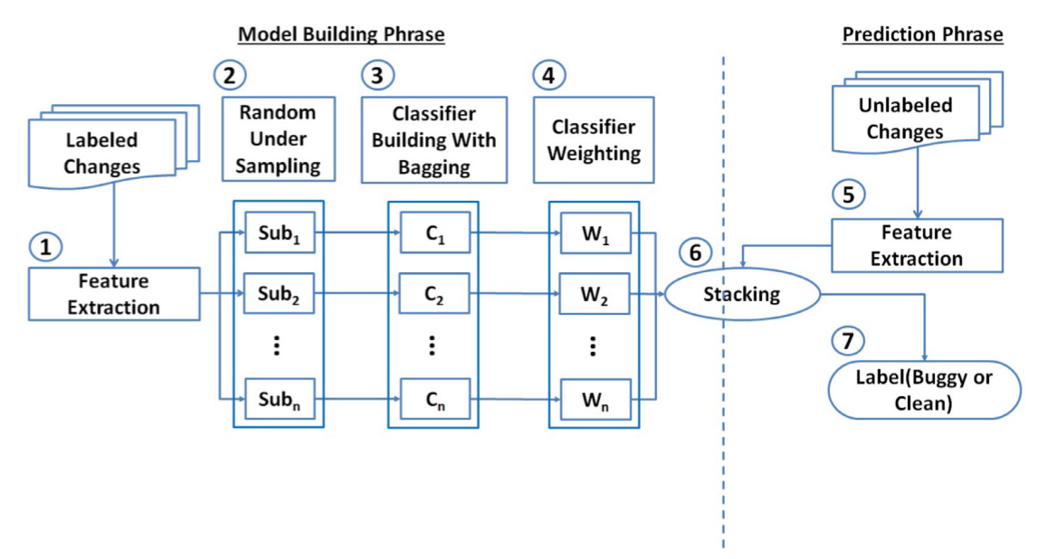
Figure 5. Two-Layer Ensemble Learning framework replicated from the work by Yang et al. (Yang et al., 2017)

5.4. No Data Methods:

In the past, Menzies et al. showed trivial approaches that use no training information like Manual Up/Down outperformed in identifying defects compared to complex methods (Menzies et al., 2010). Recently (2018) Zhou et al. reported that simple size-based models show a promising predictive performance, therefore advising researchers to include Manual Up/Down methods as a baseline while proposing any new technique (Zhou et al., 2018).

Koru et al. related a module’s defect proneness to its size. In one case with two commercial projects, they found smaller modules were defective (Koru et al., 2008a) whereas in another they found larger classes were more defect prone (Koru et al., 2008b). Therefore we include both their methods ManualDown and ManualUp to label our test commits.

5.5. ManualDown

We label all test commits as defective if the size (‘la’ in Table 4) is greater than the median size among the test commits (Zhou et al., 2018). The philosophy here is more enormous changes should be inspected first and therefore penalized.

5.6. ManualUp

We label all test commits as defective if the size (‘la’ in Table 4) is less than or equal to the median size among the test commits (Koru et al., 2008b). The philosophy here is more minor changes should be inspected first and therefore penalized.

Nature	Type	Method	Pre-processing	# Features (columns)	# of commits (rows)
		Bellwether (Krishna et al., 2016)	CFS, SMOTE and steps illustrated in §5.1	Selected by CFS.	All commits from the identified cross-project.
late-data	Cross	TCA+(Nam et al., 2013a)	SMOTE	5 components with a linear kernel (data supplied with all features)	Pick the first 150 and last 150 commits from the bellwether project.
		$*\mathit{E_{size}(Bellwether)}$	Steps illustrated in §5.1 in (Nagappan and Ball, 2005; Kamei et al., 2012; Kondo et al., 2020)	LA, LT = lines added, lines of code in the file before change	Sample an equal number of defective and clean commits as available in the first 150 commits (not exceeding 25 each).
early-data	Cross	$*\mathit{E_{size}(TCA+)}$	Steps illustrated in §5.1	2 components with the linear kernel (data supplied only with LA and LT)
		$\mathit{E}$ (Shrikanth et al., 2021)	CFS and steps illustrated in §5.1	Selected by CFS
early-data	Within	$*\mathit{E_{size}}$	Steps illustrated in §5.1	LA and LT	(same as above)
late-data	Within	$ALL$	CFS, SMOTE and steps illustrated in §5.1	Selected by CFS.	All the commits before the release, which is under test.

KEY: All early-data sampling methods are shaded () and policies proposed in this study are indicated by *.

Table 6. This table lists three baseline approaches (where two of them are Cross and the remaining one is a Within) along with three early-data variants to support this study. Note, many of these methods used the steps advised in (Nagappan and Ball, 2005; Kamei et al., 2012; Kondo et al., 2020). Those steps are discussed in §5.1. Further, for a discussion on CFS, see §5.7.

5.7. Pre-processers

Pre-processing the training and in some cases, test data has been shown very effective and necessary in building defect predictors. The following methods are representative of much of of the prior research in this field:

• The steps advised by (Nagappan and Ball, 2005; Shihab et al., 2010; Kondo et al., 2019) (see §5.1);

• Correlation-based Feature Selection (CFS);

• Synthetic Minority Over-Sampling (SMOTE).

Note: Not all combinations of pre-processing steps are valid. Table 6 show the types of pre-processing applied for each sampling policy used in this paper. Further, we avoid a common threat to validity, we state there that we applied SMOTE only to the training data but not to the test data (Agrawal and Menzies, 2018)).

5.7.1. Correlation-based Feature Selection (CFS):

CFS is a prevalent feature selection technique proposed by Hall  (Hall and Holmes, 2003). That is often used in building supervised software defect prediction models, especially while building defect predictors (Kondo et al., 2019). A heuristic-based technique to incrementally assess a subset of features. Internally, a best-first search is applied to identify influential sets of features that are not correlated with each other. Nevertheless, it should be correlated with the target (classification). Each feature subset is computed as follows: $\mathit{merit}s=\color[rgb]{0,0,0}k*r{\mathit{cf}}/\sqrt{k+k(k-1)r_{\mathit{ff}}}$ where:

• $\mathit{merit}s$ is the value of subset $s$ having $k$ features;

• $r{\mathit{cf}}$ is the score that explains the connection of that feature set to the class;

• $r{\mathit{ff}}$ is the feature to feature mean and connection between the items in $s$.

5.7.2. Synthetic Minority Over-Sampling (SMOTE):

A sampling technique proposed by Chawla et al. (Chawla et al., 2002) to handle the class imbalance problem. Because when there are an unequal number of clean and defective commits (or modules, records, etc.) in the training set, classifiers can scuffle to discover the target class. SMOTE is recommended by many researchers in the space of software defect prediction (Agrawal and Menzies, 2018; Tantithamthavorn et al., 2018).

5.8. Training Data Selection Methods

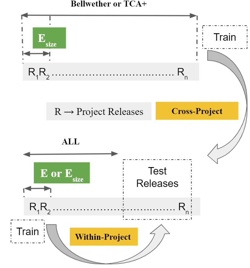
Figure 6. A visual map to gauge the sampling policies (training commits selection) listed in Table 6.

The essence of this work is how we sample data to train defect predictors and figure 6 attempts to portray the same. The figure 6 shows a set of options from which we can generate a large number of sampling options. For example, training data come from within or be drawn cross from another project. It is helpful to view figure 6 along with the selection methods listed in Table 6.

Shrikanth et al. identified many sampling strategies (based on recent releases, recent months of data, and all past data) to build predictors in the Within project context (Shrikanth et al., 2021). To find representative training data selection methods for the Cross context we checked the papers listed in Table 2. We found numerous Cross techniques reported in the past decades; for example, Sousuke’s work recently (2020) explored 24 Cross approaches (Amasaki, 2020). Overall, in the context of Cross, we found only two (‘whole’ or ‘part’). Nevertheless, both ‘whole’ and ‘part’ is late-data. As the focus of this study is to check the efficacy of using early-data approaches in prevalent Cross approaches and not rank numerous Cross techniques.

5.8.1. Cross:

We chose two representative Cross techniques, specifically $\mathit{TCA+}$ and $\mathit{Bellwether}$, because:

• $\mathit{TCA+}$ is an active Cross technique in this space based on the seminal work by Nam et al. (Nam et al., 2013a).

• $\mathit{Bellwether}$, a recent (2018) baseline approach by Krishna et al. that performed better than $\mathit{TCA+}$ (Krishna and Menzies, 2018)

Bellwether Project ($\mathit{Bellwether}$):

The bellwether transfer learning method assumes “When a community works on software, then there exists one exemplary project, called the bellwether, which can define predictors for the others. (Krishna and Menzies, 2018)”.

Transfer Component Analysis (TCA+):

Pan et al. proposed a domain adaptation technique that enables the transition of information between source and target domains (Pan et al., 2010). Extending that, Nam et al. stacked many normalization rules on top of TCA to form TCA+ (Nam et al., 2013b). A specific normalization rule is applied based on the similarity of the data set characteristics between the source and the target project. Rahul and Menzies (Krishna and Menzies, 2018) report TCA+ to perform better than other transfer methods, namely, Transfer Naive Bayes (Ma et al., 2012) and Value Cognitive Boosting Learner (Ryu et al., 2016). TCA+ can be somewhat computationally expensive. To ally that, we built defect predictions with varying sizes in our prior work (Shrikanth et al., 2021) and found that predictors needed a minimum of 150 training commits. As mentioned above unlike other methods $TCA+$ is CPU intensive, therefore we could only increase training commits up to 300 (2x 150). This is not a sampling threat because later in §6 we find the early-data-lite $TCA+$ variant performs better than $TCA+$ trained with 300 commits supporting our early conjecture. For TCA+ related policies listed in Table 6 we reused the implementation from their replication package  by Kondo et al., which is an EMSE’19 article about feature reduction techniques on software defect prediction models (Kondo et al., 2019). The above two techniques use all available cross-project data. We include two Early Cross variants specifically Early Bellwether ($\mathit{E_{size}(Bellwether)}$), Early TCA+ ($\mathit{E_{size}(TCA+)}$) that only uses early cross-project data and only two features.

5.8.2. Within:

$ALL$ uses all available past data within the project under test to predict future defects. We create two early variants ($\mathit{E}$) that use early within project data will all features (as selected by CFS) and ($\mathit{E_{size}}$) is same as $E$ except it uses only two features

For specific sampling numbers and rules please refer to Table 6.

5.9. Evaluation Criteria

We use all eight criteria used in the baseline study to gauge the predictors built using various sampling policies. That study consults from widely-used measures (Menzies et al., 2008; Wang and Yao, 2013; Tantithamthavorn et al., 2018; Bennin et al., 2019; Zhang et al., 2014; McIntosh and Kamei, 2017; Tantithamthavorn et al., 2018; Kondo et al., 2020; Yatish et al., 2019; Yan et al., 2019; Zhang et al., 2016a; D’Ambros et al., 2012; Kamei et al., 2012) in the software defect prediction literature.

5.9.1. Brier

The brier score is the mean squared error (MSE) of the actual outcome $y\in\{0,1\}$(clean or defective) and the predicted probability estimate $p=\operatorname{Pr}(y=1)$ for test commits (samples) computed as below:

(2) $$\footnotesize Brier=\frac{1}{n_{\text{samples}}}\sum_{i=0}^{n_{\text{samples}}-1}(y_{i}-p_{i})^{2}$$

Numerous software defect prediction papers (McIntosh and Kamei, 2017; Tantithamthavorn et al., 2018, 2018; Kondo et al., 2020) endorse this measure (Pedregosa et al., 2011a).

5.9.2. Initial number of False Alarms (IFA)

Based on the observation by Parnin and Orso  (Parnin and Orso, 2011) that developers lose their trust in such analytics if they encounter many initial false alarms. Thus by simply counting the number of false alarms encountered after sorting the commits in the order of probability of being defect-prone. IFA is simply the number of false alarms before finding the first actual alarm.

5.9.3. Recall

Recall is the number of inspected defective commits divided by all the defective commits.

(3) $$\footnotesize\mathit{Recall}=\frac{\mathit{True\ Positives}}{\mathit{True\ Positives+False\ Negatives}}$$

5.9.4. False Positive Rate (PF)

PF is the ratio between the number of clean commits predicted as defective to all the defective commits (irrespective of classification).

(4) $$\footnotesize\mathit{PF}=\frac{\mathit{False\ Positives}}{\mathit{False\ Positives+True\ Negatives}}$$

5.9.5. Area Under the Receiver Operating Characteristic curve (AUC)

It is simply the area under the curve between the false-positive rate and true-positive rate.

5.9.6. Distance to Heaven (D2H)

D2H or “distance to heaven” is computed as an aggregation on two metrics Recall and False Positive Rate (PF). Where “heaven” is a place with $\mathit{Recall=1}$ & $\mathit{PF=0}$ (Chen et al., 2018a).

(5) $$\footnotesize\mathit{D2H}=\frac{\sqrt{(1-\mathit{Recall})^{2}+(0-\mathit{PF})^{2}}}{\sqrt{2}}$$

5.9.7. G-measure (GM)

GM is computed as a harmonic mean between the complement of PF and Recall. It is measured as shown below:

(6) $$\footnotesize\mathit{G-Measure}=\frac{2*\mathit{Recall}*(1-\mathit{PF})}{\mathit{Recall}+(1-\mathit{PF})}$$

GM and D2H essentially combine the same two measures, $\mathit{Recall}$ and $\mathit{PF}$. Nevertheless, we still employ those as they have been used and endorsed separately in the literature. Notably, as seen from results in (Shrikanth et al., 2021) and in this work shown later in §6, it is not necessary that achieving good results on GM would also associate with good D2H (or vice-versa).

Due to the nature of the classification process, some criteria will always offer contradictory results:

• A classifier may simply achieve 100% $\mathit{Recall}$ just by labeling all the test commits as defective. But as a side-effect, that method will incur a high $\mathit{PF}$.

• Secondly, a classifier may classify all test commits as clean to show 0% $\mathit{PF}$, but that method will incur a very low $\mathit{Recall}$.

• Lastly, Brier and Recall are also antithetical since reducing the loss function implies missing some conclusions lowering $\mathit{Recall}$.

5.9.8. Mathew’s Correlation Coefficient (MCC)

MCC utilizes all the four computations namely True Positives (TP), True Negatives (TN), False Positives (FP), and False Negatives (FN) of the confusion matrix, such that:

(7) $$\footnotesize{\text{MCC}}=\frac{{\mathit{TP}}\times{\mathit{TN}}-{\mathit{FP}}\times{\mathit{FN}}}{\sqrt{({\mathit{TP}}+{\mathit{FP}})({\mathit{TP}}+{\mathit{FN}})({\mathit{TN}}+{\mathit{FP}})({\mathit{TN}}+{\mathit{FN}})}}$$

Thus, many researchers endorse the use of MCC, especially in the space of software defect prediction (Yao and Shepperd, 2020; Kondo et al., 2020). It returns a score between $-1$ and $+1$, where $+1$ indicates higher predictive performance, $-1$ contrary predictions, and $0$ indicates most of the predictions’ poor predictive performance (random).

Note for the above eight predictive performance measures:

• Initial number of False Alarms range from 0 to # (maximum number of commits inspected);

• MCC range from -1 to 1;

• D2H, IFA, Brier, PF of these criteria need to be minimized, i.e., for these criteria less is better.

• For four of these AUC, Recall, G-Measure, and MCC criteria need to be maximized, i.e., for these criteria more is better.

Prior work has shown that precision has significant issues for unbalanced data. We do not include that in our evaluation  (Menzies et al., 2008). Prior reviewers of this paper have noted that this might mean we miss certain effects relating to that section of the evaluation space. To address that point, we have added an evaluation metric that draws from multiple “corners” of the evaluation space (see the MCC measure of §5.9.8)

5.10. Statistical Tests

Predictors built using each of the sampling policies listed in Table 6 are tested on all appropriate (future) project releases. Then we compute each of the evaluation criteria discussed above in §5.9. Then each of the scores is grouped and exported by a sampling policy and classifier pair.

To reiterate, each population is a collection of a specific evaluation score. Moreover, populations can have the same median but have an entirely different distribution. Thus to rank each of those populations of evaluation scores, we use the Scott-Knott test recommended by Mittas et al. in TSE’13 paper (Mittas and Angelis, 2013). This procedure is a top-down bi-clustering method used to rank different predictors created using different sampling policies and classifiers under a specific evaluation measure. This method sorts a list of $l$ those evaluation scores $\mathit{ls}$ by their median score. Next, it then splits $l$ into sub-lists m, n. This is done to maximize the expected value of differences in the observed performances before and after divisions.

For lists $l,m,n$ of size $\mathit{ls},\mathit{ms},\mathit{ns}$ where $l=m\cup n$, the “best” division maximizes $E(\Delta)$; i.e. the difference in the expected mean value before and after the spit:

$$E(\Delta)=\frac{ms}{ls}abs(m.\mu-l.\mu)^{2}+\frac{ns}{ls}abs(n.\mu-l.\mu)^{2}$$

Additionally, a conjunction of bootstrapping and A12 effect size test by Vargha and Delaney (Vargha and Delaney, 2000) is applied to avoid “small effects” with statistically significant results.

Important note: we apply the Scott-Knott test independently to all the eight evaluation criteria; i.e., when we compute ranks, we do so for (say) $\mathit{Recall}$ separately to $\mathit{PF}$. In the rest of this paper, when we say ‘similar’, we mean the distributions in comparison belong to the same Scott-Knott rank (ie., clustered in the same group), and when we say ‘better’ we mean the distribution is statistically different (ie., cannot be clustered into the same group) and favorable (eg., higher $Recall$ or lower $PF$).

5.11. Other Details

We wish to report not just performance scores but also offer some details about the model that generates those scores. To that end, we will exploit the bellwether effect. Specifically, we will (a) find the most important features, then (b)  use them in bellwethers that represent most of our data.

6. Results

An overview of our experiments is shown in Figure 6. We build defect predictors using the sampling strategies listed in Table 6 and classifiers elucidated in §5.2. Then, similar to our prior work (Shrikanth et al., 2021) we test the built defect predictors in all the project releases .

In this paper, the results of RQ1 are used in RQ2 and so on to eliminate redundant assessment and comparison of treatments. Therefore, we eliminate treatments (defect predictors) that are either already been assessed or when they do not affect the conclusion of the RQ under investigation. We do this to eliminate redundancy in analysis and improve brevity in our results. For instance, we do not build defect predictors using training commits based on recent data (since it was assessed in prior work against early-bird heuristic (Shrikanth et al., 2021)).

6.1. RQ1: Can we build early software defect prediction models from unpopular projects?

6.1.1. Motivation

Our prior results that endorsed early methods were scoped to only popular GitHub projects (Shrikanth et al., 2021). Choosing only popular projects is a sampling decision often made by many SE researchers in empirical studies to mitigate generalizability threat (Munaiah et al., 2017). As mentioned earlier in §5.1, unpopular projects could be non-trivial projects (like homework assignments), and that could affect the conclusion.

On the contrary, a strong argument could be that perhaps popular projects may not realistically represent SE in the real world. In other words, not all projects are fully staffed with a sufficient budget. Therefore it is necessary and worthy to check the value of early methods on the unpopular sample of projects. To reiterate, in §5.1 we elucidate the selection criterion of unpopular and non-trivial SE projects from GitHub. Later in §7 we discuss how we mitigated GitHub projects sampling threats.

6.1.2. Approach

To check whether the proposed early method work on unpopular projects we compare defect predictors built by sampling training commits using $E$ with those that sampled all past data ie., $ALL$. We do not consider other stratification like the release, or 3 months since $ALL$ subsumes more data. Notably, $ALL$ is a prevalent (50%) sampling methods in software defect prediction (Shrikanth et al., 2021). Therefore to assess defect predictors on each project release we construct the experiment as follows:

• First we sample training data within the project. The sampling will depend upon either $E$ or $ALL$.

• The sampled training data is pre-processed and appropriate features are selected as listed in Table 4.

• Classifiers listed in §5.2 are instantiated with copies of pre-processed training data.

• All the instantiated predictors are tested on all 85 unpopular project releases and their predictive performance is gauged using 7 measures elucidated in §5.9.

• Lastly, their scores (eg., the population of recall scores) per classifier+policy (pair) is ranked using the Scott-Knott test elucidated in §5.10.

To avoid a methodological error, we avoid overlap of train and test commits. For instance, we do not test on project releases before the first 150 commits. Notably, the population of evaluation measures (e.g, $Recall$) is tested on an equal number of unpopular project releases.

6.1.3. Results

To reiterate, we wanted to check if our early-bird effect identified in our prior work also holds among unpopular GitHub projects (Shrikanth et al., 2021). The results shown in Table 7 support our early-bird heuristic even among unpopular GitHub projects because the policy $E$ uses fewer early data (row #1) and performs just as same as predictors that were built sampled with $ALL$ (all past commits) in row #3.

Table 7. ‘12’ within-project software defect prediction models tested ‘only’ in 85 unpopular project’s releases. In the first row, “+” and “-” denote the criteria that need to be maximized or minimized, respectively. All the other rows show combinations of sampling policies and classifiers. Green cells denote “early-data” sampling was employed. Cells marked in gray all have the same top rank as the best results (and those ranks were determined by the Scott-Knott algorithm described in §5.10). The ‘wins’ column (see column #3) counts how often a particular sampling policy/classifier achieves a top score. Inter-quartile ranges are indicated within ‘( )’.

Policy	Classifier	Wins	Recall+	PF-	AUC+	D2H-	Brier-	G-Score+	IFA-	MCC+
E	LR	6	75 (50)	40 (34)	64 (17)	41 (22)	38 (22)	65 (27)	1 (4)	24 (28)
E	SVM		69 (50)	38 (30)	64 (18)	41 (21)	37 (21)	63 (30)	1 (4)	23 (31)
ALL	SVM		50 (54)	15 (18)	65 (25)	40 (32)	23 (14)	54 (51)	1 (5)	28 (45)
ALL	RF		50 (52)	16 (22)	64 (22)	42 (28)	25 (16)	53 (46)	1 (4)	28 (41)
ALL	KNN		50 (43)	20 (17)	64 (21)	40 (25)	26 (14)	54 (41)	1 (4)	26 (38)
E	KNN	5	67 (40)	42 (26)	62 (19)	42 (19)	40 (17)	61 (28)	2 (5)	19 (30)
E	RF	4	56 (52)	28 (28)	63 (20)	42 (23)	33 (18)	56 (39)	2 (5)	23 (33)
ALL	NB	2	14 (60)	9 (27)	50 (13)	64 (24)	25 (22)	14 (51)	4 (12)	1 (30)
E	NB	1	56 (66)	35 (38)	56 (19)	48 (25)	38 (24)	52 (47)	2 (6)	14 (32)
ALL	LR		50 (80)	25 (28)	60 (19)	47 (37)	30 (20)	51 (69)	2 (7)	17 (36)
E	DT		50 (53)	32 (31)	57 (19)	47 (27)	37 (23)	52 (46)	2 (6)	14 (33)
ALL	DT		50 (38)	30 (23)	57 (18)	45 (23)	34 (18)	51 (35)	2 (5)	15 (34)

6.2. RQ2: Can we build early software defect prediction models with fewer features?

6.2.1. Motivation

The prior work showed that it is possible to build operable defect predictors using fewer early project data. One reason for the preceding work was that much of the knowledge required (defects) to build defect predictors were reported within a few months of the project. In this work, we explore that region again to understand which of those 14 features listed in Table 4 are essential to the early predictor $E$. And if the answer to that is a few, can we restrict the predictors to only learning from a fixed set of features while producing operable performance? It would be easier to explain with fewer features why a specific commit was classified as defective by the predictor.

6.2.2. Approach

To answer this RQ we perform three experiments as follows:

• In the first experiment we report the frequency of features chosen by CFS while building defect predictors which were sampled using $E$.

• In the second experiment we create a new sampling policy (say $E_{?}$) that only uses the most frequently chosen feature identified in the above step.

• We create two predictors that sampled training commits (pre-processed as listed in Table 6) using $E$ and $E_{?}$ and test on all project releases.

• In the third experiment, we also test all project releases using the ManualUp and ManualDown approach (elucidated in §5.2) that uses no training information. This is because researchers have advised including such trivial approaches that do not use any training information (Zhou et al., 2018).

• Lastly, we compare the predictive performance of defect predictors that were built using $E$, $E_{?}$ and $ManualDown$ and $ManualUp$ on all eight evaluation measures listed in §5.9 and rank them using the Scott-Knott test elucidated in §5.10.

6.2.3. Results

We make the following observations from Figure 7 and Table 8:

Finding Important Features:

Shrikanth et al.’s early sampling rule ‘E’ is shown to be adequate for Within (Shrikanth et al., 2021). Given that we are building models from such a sample, it is tempting to ask, “does that small sample produce a succinct model?”. Note that if this was indeed the case, then we could offer a clear report on what factors most influence defects.

Figure 7 shows the frequency of features selected by the CFS algorithm (see §5.7) across all our 240 projects (using just the first 150 commits). To select the “best” features from that space, we build models using the top $1\leq x\leq 12$ ranked features, stopping with $x+1$ features performed no better than $x$ features (and here, we are testing all the releases that occurred after that first 150 commits). That procedure reported that models learned from two size-ranked features performed as well as anything else:

• LA: Lines of code added

• LT: Lines of code in a file before the change

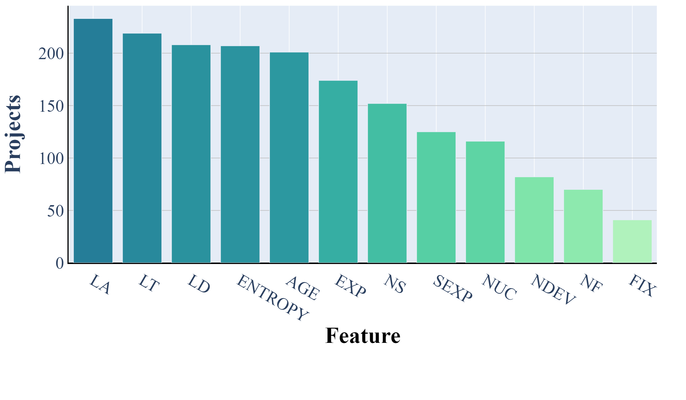
Figure 7. Frequency of features chosen by the CFS feature selector (using just the first 150 commits) sampled using $\mathit{E}$ in all the 240 projects

Using the results from Figure 7 we built an early defect predictor only using the top two features ‘LA’ and ‘LT’. Therefore $E_{?}$ becomes $E_{size}$. The results from Table 8 clearly show that $E_{size}$ have more wins than predictors that sampled training commit using $E$. And by extension to prior result $ALL$ or other stratification like recent release or based on months. While $ManualDown$ is seen at the top of the table due to higher recall, it also produced many false alarms (see row #3 where $PF$ is 48%).

Table 8. ‘14’ within-project software defect prediction models tested in all 240 project releases. In the first row, “+” and “-” denote the criteria that need to be maximized or minimized, respectively. All the other rows show combinations of sampling policies and classifiers. Green cells denote “early-data” sampling was employed. Cells marked in gray all have the same top rank as the best results (and those ranks were determined by the Scott-Knott algorithm described in §5.10). The score highlighted in bold red text indicates undesirable PF, despite many wins on other evaluation measures. The ‘wins’ column (see column #3) counts how often a particular sampling policy/classifier achieves a top score. Inter-quartile ranges are indicated within ‘( )’.

Policy	Classifier	Wins	Recall+	PF-	AUC+	D2H-	Brier-	G-Score+	IFA-	MCC+
$E_{size}$	LR		75 (40)	28 (25)	70 (15)	34 (17)	30 (17)	70 (25)	1 (3)	34 (26)
$E_{size}$	SVM		73 (44)	30 (27)	69 (15)	35 (19)	30 (18)	69 (26)	1 (3)	33 (27)
-	$ManualDown$	6	86 (25)	48 (15)	70 (12)	36 (11)	41 (17)	75 (14)	1 (4)	30 (22)
$E_{size}$	KNN	4	70 (41)	33 (26)	67 (17)	37 (19)	33 (18)	66 (26)	1 (3)	28 (28)
$E_{size}$	NB		75 (53)	38 (41)	63 (17)	44 (23)	36 (25)	61 (35)	1 (4)	24 (31)
E	LR		70 (42)	37 (33)	63 (16)	41 (22)	36 (20)	62 (30)	1 (4)	24 (28)
E	SVM		67 (42)	33 (31)	64 (17)	40 (20)	34 (19)	63 (30)	1 (4)	25 (28)
E	KNN		66 (43)	38 (30)	62 (18)	42 (20)	37 (20)	59 (28)	1 (4)	21 (31)
$E_{size}$	RF		64 (40)	31 (30)	64 (17)	40 (20)	33 (18)	61 (28)	1 (4)	25 (30)
$E_{size}$	DT		62 (39)	38 (30)	61 (18)	43 (19)	38 (20)	57 (28)	1 (4)	19 (32)
E	RF		60 (46)	32 (33)	61 (18)	43 (21)	35 (21)	56 (33)	1 (4)	20 (32)
E	DT		56 (46)	41 (37)	56 (17)	49 (22)	41 (24)	52 (33)	2 (5)	11 (30)
E	NB	2	50 (75)	27 (48)	54 (14)	55 (30)	36 (26)	38 (62)	2 (7)	8 (26)
-	$ManualUp$	0	14 (25)	52 (15)	30 (12)	73 (11)	59 (17)	16 (27)	7 (13)	-30 (22)

6.3. RQ3: Can we build early software defect prediction models from transferring early life cycle data from other projects?

6.3.1. Motivation

§5.8 lists both the situations and challenges of when one might need to transfer project data to build defect predictors. Although we cannot solve all Cross-project challenges in one article, we could pacify some of them by checking the efficacy of early methods in this context. If early methods work, then we can transfer relevant data from vast search space (many projects) in less time. Further, we can also reduce the need for data availability as we will only need a small portion of early data.

6.3.2. Approach

To check the efficacy of Cross-project methods against early methods we will build predictors using the following sampling strategies below:

• Cross-project methods $Bellwether$ and $TCA+$

• We created early variants of Cross-project methods $Bellwether$ and $TCA+$ namely $E_{size}(Bellwether)$ and $E_{size}(TCA+)$. The details of these sampling strategies are elucidated in Table 6 and portrayed visually in Figure 6.

• We also include the within-project $E_{size}$ to compare Cross and Within.

• Note: We do not include $ALL$ or $E$ because $E_{size}$ outperformed those sampling strategies in Table 8 and in our prior result (Shrikanth et al., 2021).

The Cross-projects methods require a representative project among the 240 projects to transfer data from.

Finding Representative Cross-Project:

Using just LA and LT for each of our projects, we found a model and measured its performance on the other projects. If that median performance was more the 70% ‘Recall’ and less than 30% ‘PF’, then the model was deemed “satisfactory”. In a result that endorses the use of early life cycle data, Figure 8 shows that more of the models found via the $E_{size}$ method was “satisfactory” than those found using all the data. That effect is particularly marked in the popular projects .

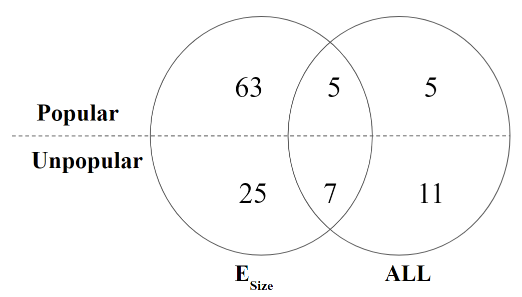
Figure 8. Number of “satisfactory” bellwethers identified independently by two different sampling policies in all 240 projects.

Lastly like in previous RQs we compare the predictive performance of the various defect predictors that were built using different sampling policies on all eight evaluation measures listed in §5.9 and rank them using the Scott-Knott test elucidated in §5.10.

Note: We avoid the methodological error of testing the representative Cross-project in this experiment.

6.3.3. Results

Figure 9. Time taken (log-scale) to identify qualifying bellwether projects in all 240 projects using $\mathit{Bellwether}$ and $\mathit{E_{size}(Bellwether)}$ policies. Note that in our experiments, we ran on a multi-core cloud-based CPU farm. To collect the data here (which assumes we are running on a single-core machine), we summed the CPU time across all the cores in our experimental rig. We assert that this sum is valid since, in our experiments, there is nearly no communication between the cores (except that very end to accumulate the results).

Figure 10. Time taken by different sampling policies to train a model based on the number of commits.

We make the following observations using Table 9, Figure 9 and Figure 10.

• Rows #1 and #2 top of the Table 9 confirm that it is better to build Cross based predictors using early-data-lite method $E_{size}$ than using sampling strategies that use more data (like $TCA+$ or $Bellwether$).

• Figure 9 and Figure 10 shows that it is much faster to identify and build bellwethers from a large pool of projects using $E_{size}$ than $Bellwether$. This is because $E_{size}$ based predictors need not update (re-train) by accumulating newer project commits for every new project release.

• Row #6 of Table 9 is the position of our prior result (Shrikanth et al., 2021) that builds predictors using Within $E$ project commits. That proves to show that we can do better than local data if we find good bellwethers.

Table 9. ‘30’ cross-project and ‘1’ within-project (denoted as $\implies$) software defect prediction models tested in all 240 project’s releases. In the first row, “+” and “-” denote the criteria that need to be maximized or minimized, respectively. All the other rows show combinations of sampling policies and classifiers. Green cells denote “early-data” sampling was employed. Cells marked in gray all have the same top rank as the best results (and those ranks were determined by the Scott-Knott algorithm described in §5.10). The ‘wins’ column (see column #3) counts how often a particular sampling policy/classifier achieves a top score. Inter-quartile ranges are indicated within ‘( )’.

Policy	Classifier	Wins	Recall+	PF-	AUC+	D2H-	Brier-	G-Score+	IFA-	MCC+
$E_{size}$ (Bellwether)	SVM		91 (26)	40 (34)	70 (16)	35 (21)	35 (23)	74 (23)	1 (4)	32 (26)
$E_{size}$ (TCA+)	SVM		88 (33)	38 (28)	70 (16)	35 (19)	34 (21)	74 (24)	1 (4)	32 (26)
$E_{size}$ (Bellwether)	LR	6	85 (30)	34 (27)	73 (15)	31 (17)	31 (18)	76 (20)	1 (4)	35 (25)
$E_{size}$ (TCA+)	LR		82 (36)	32 (25)	72 (16)	33 (19)	31 (19)	74 (22)	1 (4)	34 (26)
$E_{size}$ (TCA+)	KNN		79 (50)	32 (25)	70 (18)	35 (20)	32 (18)	72 (28)	1 (5)	30 (28)
$\implies$ $E_{size}$ (Within)	LR		78 (43)	25 (25)	73 (16)	31 (18)	27 (18)	73 (28)	1 (3)	37 (27)
$E_{size}$ (Bellwether)	KNN		78 (43)	30 (26)	70 (17)	34 (19)	30 (19)	72 (27)	1 (3)	32 (27)
$E_{size}$ (TCA+)	RF	5	75 (46)	31 (24)	69 (17)	35 (19)	32 (18)	71 (28)	1 (4)	30 (28)
$E$ (TCA+)	LR	4	80 (40)	41 (19)	69 (16)	36 (15)	38 (17)	72 (24)	2 (5)	28 (27)
$E_{size}$ (Bellwether)	RF		71 (41)	28 (26)	68 (18)	36 (21)	30 (19)	67 (28)	1 (4)	28 (28)
Bellwether	SVM		21 (44)	4 (10)	57 (17)	56 (30)	19 (15)	25 (49)	1 (7)	23 (40)
Bellwether	RF	3	19 (36)	3 (8)	56 (15)	56 (25)	19 (15)	23 (41)	1 (7)	22 (39)
$E_{size}$ (Bellwether)	NB		88 (33)	49 (34)	64 (19)	42 (22)	42 (23)	67 (28)	2 (5)	23 (27)
$E_{size}$ (TCA+)	NB		82 (38)	43 (30)	67 (18)	39 (21)	38 (22)	70 (26)	2 (5)	25 (28)
Bellwether	LR		76 (51)	33 (43)	67 (16)	39 (20)	32 (24)	66 (34)	1 (4)	31 (28)
$E_{size}$ (TCA+)	DT		71 (39)	32 (25)	67 (19)	37 (19)	33 (18)	67 (27)	2 (4)	27 (28)
Bellwether	KNN	2	25 (41)	6 (10)	59 (17)	53 (27)	20 (16)	28 (44)	1 (5)	24 (39)
$E$ (TCA+)	KNN		71 (53)	37 (28)	64 (20)	40 (21)	36 (20)	65 (33)	2 (5)	23 (28)
$E$ (TCA+)	SVM		70 (55)	34 (31)	64 (20)	41 (24)	35 (21)	64 (40)	2 (5)	23 (32)
TCA+	LR		70 (39)	50 (22)	61 (22)	42 (21)	45 (22)	64 (28)	2 (6)	17 (35)
$E$ (TCA+)	NB		67 (56)	39 (38)	60 (20)	46 (24)	38 (24)	60 (44)	2 (6)	17 (32)
$E_{size}$ (Bellwether)	DT		67 (44)	30 (26)	65 (20)	39 (23)	33 (19)	63 (32)	1 (4)	25 (32)
$E$ (TCA+)	DT		67 (42)	37 (25)	63 (19)	41 (20)	38 (18)	62 (30)	2 (5)	20 (30)
$E$ (TCA+)	RF		67 (40)	34 (23)	65 (20)	38 (19)	35 (18)	65 (28)	2 (5)	24 (28)
Bellwether	NB		50 (60)	15 (21)	64 (22)	41 (32)	25 (16)	53 (55)	1 (5)	26 (38)
TCA+	SVM		50 (50)	23 (27)	61 (21)	45 (25)	31 (21)	52 (41)	2 (5)	20 (34)
TCA+	RF		50 (50)	31 (32)	57 (17)	48 (23)	36 (23)	49 (36)	2 (6)	13 (28)
TCA+	DT		50 (40)	34 (28)	56 (17)	49 (21)	39 (21)	48 (31)	2 (6)	11 (28)
TCA+	KNN		40 (42)	19 (22)	57 (18)	49 (24)	28 (21)	42 (36)	2 (5)	16 (32)
Bellwether	DT	1	33 (33)	13 (12)	59 (16)	48 (21)	24 (16)	38 (34)	1 (5)	19 (32)
TCA+	NB	0	23 (47)	19 (35)	50 (14)	61 (22)	34 (28)	23 (48)	3 (9)	0 (28)

6.4. RQ4: Do complex methods supersede early software defect prediction models ?

6.4.1. Motivation

Our prior work and RQs 1, 2, and 3 have used classifiers with default parameter settings (off the shelf). However, numerous studies, especially in the space of software defect prediction, have shown considerable improvement in predictive performance when the classifiers are tuned (Fu et al., 2016; Agrawal et al., 2019) or using an ensemble approach (Yang et al., 2017). But note the downside of tuning is the run-time overhead.

Therefore, it is essential to check if complex methods like tuning or ensemble favor sampling policies that use recent (or more) data than those confined to the early regions. It is also motivating to check if early methods can benefit from these complex methods. Perhaps the run-time overheads can be alleviated by working with fewer early data.

6.4.2. Approach

We build predictors using the state-of-the-art methods, specifically $DODGE$, $Hyperopt$, and $TLEL$ elucidated in §5.2. RQ’s 1 to 3 in either Within or Cross context $E_{size}$ has performed similar or better than prevalent sampling strategies, indicating the importance of early regions of the software project. Therefore like RQ#3 we create variants of $DODGE$ , $Hyperopt$ and $TLEL$ using $E_{size}$. In other words, we will input fewer early data $E_{size}$ and use those complex methods to check if they perform better or worse.

The optimizers $DODGE$ and $Hyperopt$ find the best set of hyper-parameters using the commits sampled according to the policy rule (specified in Table 6) to minimize $D2H$ score (elucidated in §5.9). We do not sample tuning commits separately; the optimizers sample the tuning commits within the training commit boundary defined by the sampling policy. We note here that we tried to use 50% of the training commits for training and the rest for tuning and used 100% of the commits for both training and tuning; neither stratification impacted the optimizer results.

Since the optimizers have a huge run-time overhead, and our sample includes projects with over 10,000 commits (for e.g., homebrew-cask has 98,362 commits). Therefore, it is not feasible to test many large models repeatedly on over 10,000+ releases across multiple classifiers. On the other hand, data should not be scarce for optimizers to learn tuning parameters effectively. Hence, we limit optimizers to use up to 957 commits (in the case of $ALL$). This is because, in, RQ1 we confirmed that the project’s popularity has no impact on the results. Hence, we use the median commits (957) of the unpopular projects (see Figure 2(b)), which we think is a reasonable representation of the whole population.

Lastly, we measure the predictive performance of the above approaches listed in §5.9 and rank the predictive performance of defect predictors that were built using the Scott-Knott test elucidated in §5.10.

6.4.3. Results

We make the following observations from Table 10:

• $E_{size}$ (row #1) performs better than all complex methods that use either more data $ALL$ or fewer early date $E_{size}$.

• Closest to $E_{size}$ is the two-layer ensemble method that achieves almost similar results but with more data and more processing. But note $TLEL$ (row #2) was trained on every new project release accumulating more data, whereas $E_{size}$ or any $E$ based method is always trained just ‘once’.

Table 10. 7 within-project software defect prediction models tested in all 240 project releases. In the first row, “+” and “-” denote the criteria that need to be maximized or minimized, respectively. All the other rows show combinations of sampling policies and classifiers. Green cells denote “early-data” methods (and all other rows employ an optimizer or ensemble approach). Cells marked in gray all have the same top rank as the best results (and those ranks were determined by the Scott-Knott algorithm described in §5.10). The ‘wins’ column (see column #3) counts how often a particular sampling policy/classifier achieves a top score. Inter-quartile ranges are indicated withing ‘( )’.

Policy	Classifier	Wins	Recall+	PF-	AUC+	D2H-	Brier-	G-Score+	IFA-	MCC+
$E_{size}$	LR	7	73 (43)	28 (26)	70 (15)	34 (18)	30 (17)	69 (26)	1 (3)	35 (27)
ALL	TLEL		74 (50)	36 (56)	61 (20)	46 (31)	36 (31)	54 (46)	1 (4)	21 (38)
$E_{size}$	TLEL		67 (38)	33 (30)	64 (17)	39 (19)	34 (19)	62 (27)	1 (4)	26 (30)
$E_{size}$	HyperOpt	2	27 (60)	11 (31)	54 (14)	56 (28)	28 (22)	28 (55)	2 (11)	10 (28)
$E_{size}$	DODGE		100 (80)	68 (91)	50 (7)	71 (17)	49 (46)	0 (42)	3 (9)	0 (18)
ALL	DODGE	1	100 (80)	98 (69)	50 (0)	71 (3)	66 (36)	0 (17)	4 (9)	0 (0)
ALL	HyperOpt	0	50 (89)	40 (66)	50 (9)	63 (21)	44 (30)	27 (53)	3 (9)	0 (21)

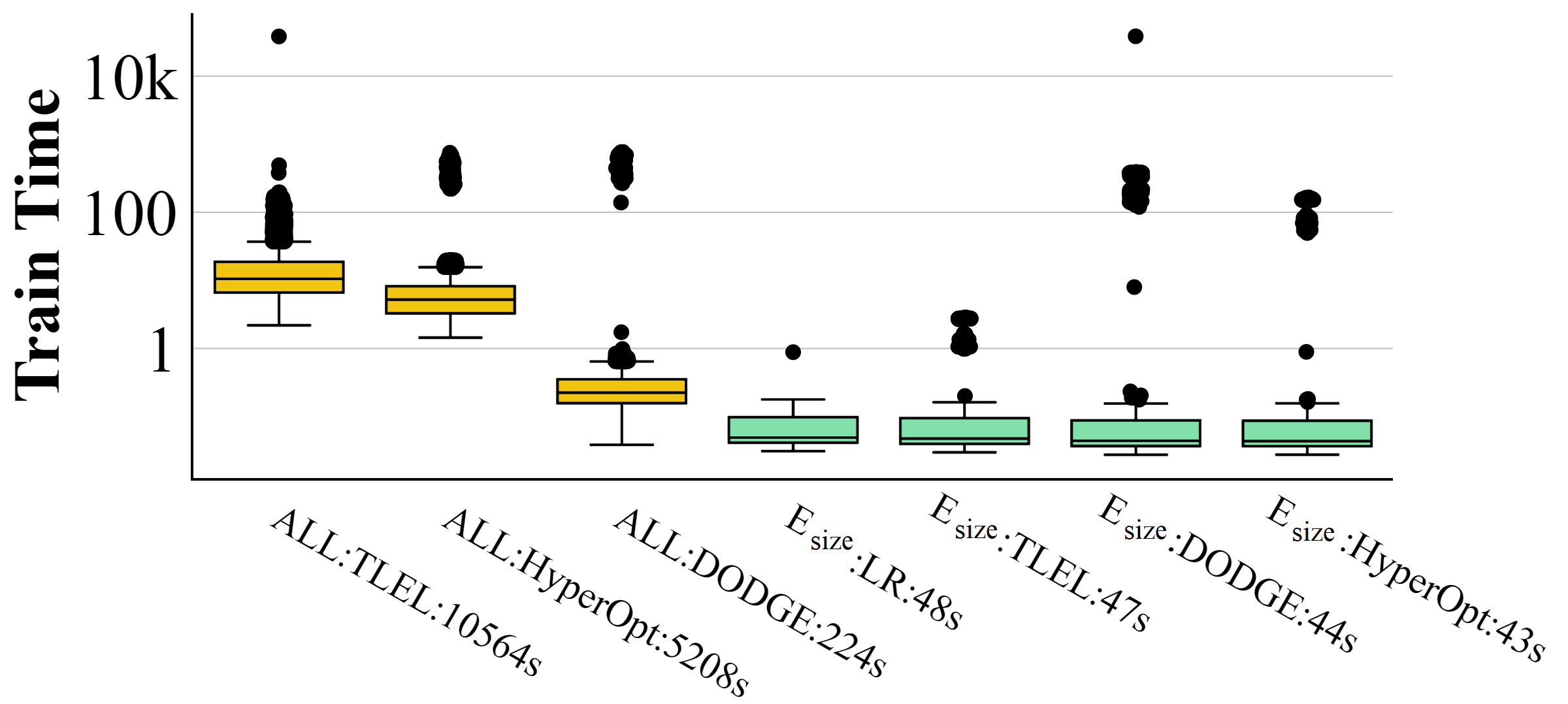
Figure 11. Time taken by different sampling policies to train a model based on the number of commits.

Notably, Figure 11 confirms it is far more faster to build predictors sampled using $E_{size}$ that neither needs SMOTE or CFS and only trained once throughout the project life cycle.

7. Threats to Validity

7.1. Sampling Bias

Generalizability of the conclusions will rely on the examples considered; i.e., what is essential here may not be genuine all over. Although the prevalent practice of such empirical studies is to use popular OS GitHub projects, we broaden the scope by including unpopular projects. Nevertheless, all these projects are non-trivial engineering projects developed in numerous programming languages for various domains. Notably, lessons did not vary in either of these two populations of projects.

7.2. Construct Validity

We mined the project samples using Commit-Guru. Commit-Guru determines risky Commits using a method similar to SZZ (Śliwerski et al., 2005). Such an approach despite its prevalence is widely debated for its false positives. To minimize that threat Commit-guru only considers files that are source-code files and not documents like readme or pdf files. Commit-Guru classifies commit into different categories one of them is merge-commit. Studies have shown merge commits have little to no influence over making real changes to the software, therefore in this study, we filter all merge commits.

Lastly, to further bold the validity of our early effect we cross-checked our results with the two projects ‘QT’ and ‘OPENSTACK’ used in the 2017 TSE article by McIntosh and Kamei (McIntosh and Kamei, 2017) and found our early trend and effect to hold. Please see the early trend of those two projects in Figure 12 and the results in Table 11. Table 11 shows results of defect predictors that sampled training commits using the recent six months (M6) endorsed in  (McIntosh and Kamei, 2017) versus $E_{size}$ endorsed in this study. Note our results are compared with ten classifiers and eight evaluation measures.

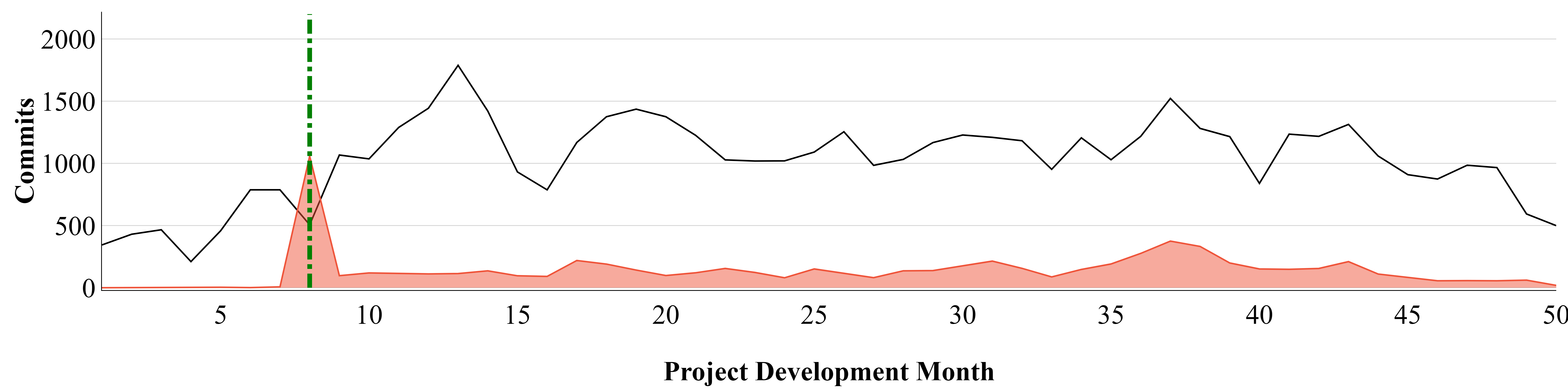
Figure 12. A repeated pattern where most defects (shaded in red) occur early in the life cycle (before the green dotted line) is also observed among the two projects (QT and OPENSTACK systems) with 37,524 commits assessed recently by McIntosh and Kamei in  (McIntosh and Kamei, 2017).

Table 11. ‘12’ within-project software defect prediction models tested ‘only’ in two projects ‘QT’ and ‘OPENSTACK’. In the first row, “+” and “-” denote the criteria that need to be maximized or minimized, respectively. All the other rows show combinations of sampling policies and classifiers. Green cells denote “early-data” sampling was employed. Cells marked in gray all have the same top rank as the best results (and those ranks were determined by the Scott-Knott algorithm described in §5.10). The ‘wins’ column (see column #3) counts how often a particular sampling policy/classifier achieves a top score. Inter-quartile ranges are indicated within ‘( )’.

Policy	Classifier	Wins	Recall+	PF-	AUC+	D2H-	Brier-	G-Score+	IFA-	MCC+
$E_{size}$	RF	6	71 (13)	35 (8)	67 (7)	33 (6)	35 (8)	69 (10)	5 (7)	19 (9)
$E_{size}$	NB	5	75 (14)	43 (7)	67 (9)	35 (7)	42 (8)	71 (9)	6 (8)	17 (10)
$E_{size}$	SVM		67 (18)	33 (9)	67 (7)	34 (8)	33 (8)	66 (14)	4 (7)	18 (11)
$E_{size}$	LR	4	64 (16)	27 (7)	67 (8)	33 (8)	28 (6)	65 (12)	4 (8)	21 (11)
$M6$	SVM		14 (25)	6 (5)	54 (10)	61 (17)	13 (7)	17 (28)	3 (8)	9 (16)
$M6$	RF	3	13 (19)	4 (5)	55 (8)	61 (13)	9 (10)	16 (22)	3 (8)	11 (17)
$M6$	KNN	2	20 (13)	8 (6)	56 (7)	56 (9)	13 (8)	24 (14)	3 (7)	11 (13)
$E_{size}$	DT		67 (18)	48 (6)	59 (7)	42 (6)	47 (5)	63 (11)	7 (9)	8 (10)
$E_{size}$	KNN		65 (17)	35 (18)	65 (7)	36 (7)	35 (16)	65 (13)	5 (9)	16 (10)
$M6$	DT		25 (21)	12 (12)	55 (7)	54 (12)	15 (14)	28 (22)	4 (11)	8 (11)
$M6$	NB	1	14 (22)	9 (12)	52 (8)	62 (12)	17 (11)	17 (21)	6 (13)	5 (13)
$M6$	LR	0	10 (28)	10 (13)	51 (6)	64 (17)	17 (12)	12 (28)	9 (52)	1 (10)

7.3. Learner bias

For identifying bellwethers by all-pairs experiment (each project is tested on all 12,000+ releases), we used only one classifier, ‘Logistic Regression.’ Perhaps other classifiers may qualify other projects are bellwethers. Using just one classifier may not be a threat for the following two reasons. Firstly a Logistic-Regression is recommended in the baseline study (Shrikanth et al., 2021) and widely endorsed in classifiers in software defect prediction literature. Secondly, in all our results in §6 Logistic-Regression based predictors were in-par and better than five other classifiers explored in this study.

Further, an empirical study can only focus on a handful of representative classifiers. Thus we chose ten classifiers (Logistic Regression, Nearest neighbor, Decision Tree, Random Forrest, and Naïve Bayes). These ten classifiers cover a broad range of classification algorithms (Ghotra et al., 2015).

7.4. Evaluation bias

This paper uses both ‘Recall’ and ‘PF’ to identify bellwethers and eight evaluation measures (Recall, PF, IFA, Brier, GM, D2H, MCC, and AUC) to compare the policies extensively. Other widely used measures in software defect prediction are precision and f-measure. However, as mentioned earlier, those threshold-dependant metrics have issues with unbalanced data (Menzies et al., 2008).

7.5. Input Bias

All our proposed sampling policies randomly sample 50 commits from the first 150 commits of the project. Along these lines, it could be true that different executions could yield different results. However, this is not a threat, as our conclusions hold on a large sample size of 12,000+ releases.

8. Discussion

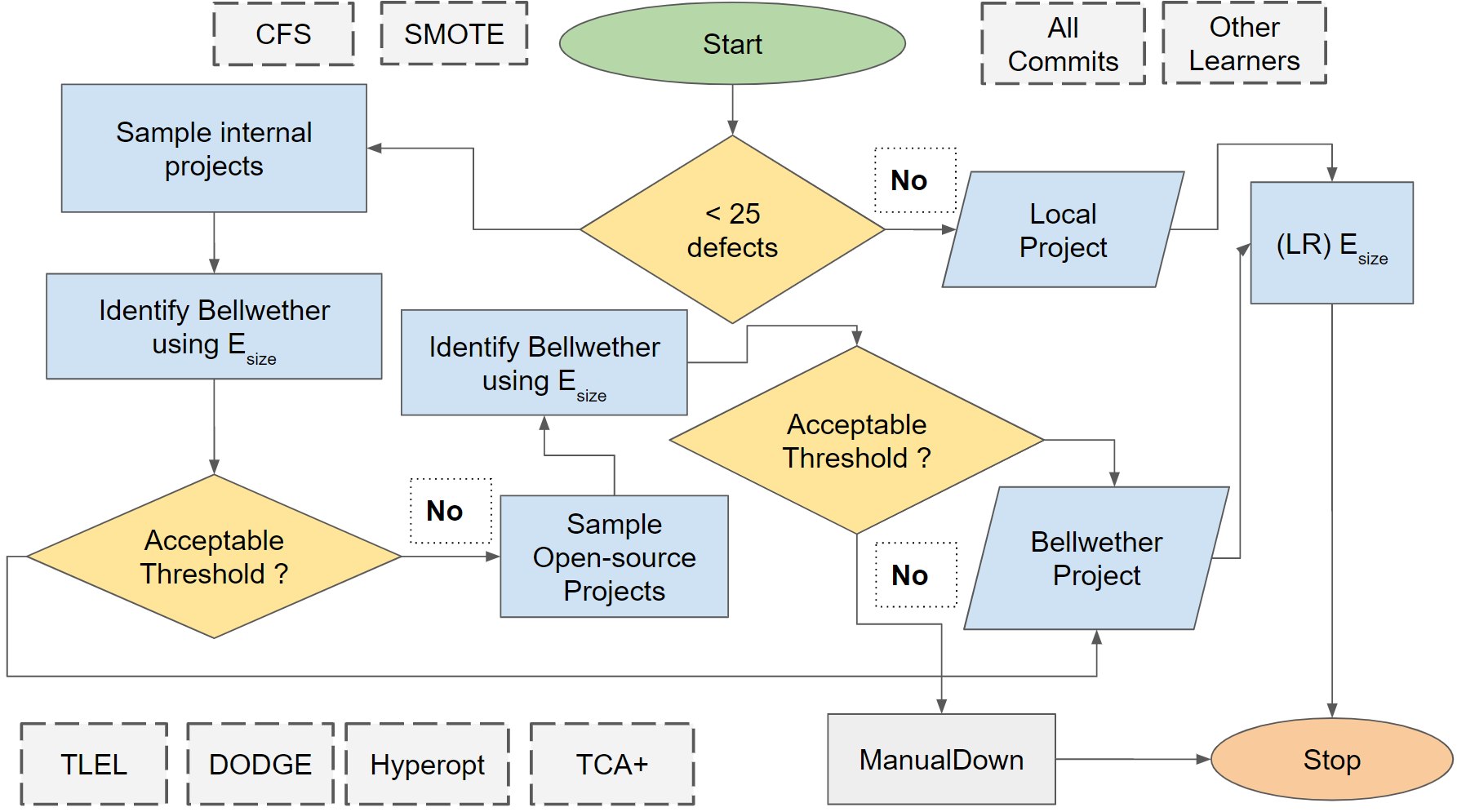
Figure 14. A decision tree to build defect predictors drawn using the results from §6 that find many complex methods (shown as disconnected blocks with dashed borders) to be needless.

We summarized the results from RQ1 to RQ4 as a simple decision tree drawn in Figure 14. The first rule in the tree eliminated the data-hungry approaches listed in Table 2 by showing that the project under test only requires 25 clean and 25 defective commits to predict post-release defects. The results of this work endorse that practitioners can quickly build an un-tuned $E_{size}$ and $LR$ defect predictor based on two size-based features. More importantly, researchers should use the early-bird treatment as a baseline before trying sophisticated methods.

In the absence of defective commits, the decision tree suggests seeking other projects from the same organization to find a suitable $Bellwether$ project. While $Bellwether$ is not a novel technique, the brute-force process of finding bellwethers can be very expensive as shown in Figure 9. This work pacifies the O($n^{2}$) process by only looking at the first 150 commits (constant) in each of the bellwether project populations of size ‘n’. If other projects from the same organization are unavailable due to issues such as data sensitivity, the tree endorses the use of open-source projects to find a suitable bellwether(s).

In situations when there is no access to data or the inability to find good bellwether projects, we suggest practitioners use $ManualDown$ until their local or other projects from the same organization report more defects ( $>24$ ). Based on the results of the RQs we find the complex tuning/ensemble methods and data-hungry sampling methods were needless and thus they are disconnected from the main flow.

8.1. Management Implications

Much prior research has struggled to find stable conclusions that hold across multiple projects. Menzies et al. warn that many global lessons (generalizations) are not supported locally (Menzies et al., 2011). That is to say, the more data we see, the more exceptions and special cases might appear in the models learned from that data. Such conclusion instability in SE has been often recorded in (Zimmermann et al., 2009; Menzies et al., 2011; Shrikanth and Menzies, 2020).

Is that the best we can do? Ideally, SE research can offer stable general software defect prediction principles (such as those seen above) to guide project management, software standards, education, tool development, and legislation about software. Such conclusion stability would have benefits for trust, insight, training, and tool development.

Trust: Conclusion instability is unsettling for project managers. Hassan (Hassan, 2017) warns that managers lose trust in software analytics if its results keep changing. But if we can find stable conclusions (e.g., using early life cycle bellwethers), that would give project managers clear guidelines on many issues, including (a) when a certain module should be inspected; (b) when modules should be refactored; and (c) deciding where to focus on expensive testing procedures.

Insight: Sawyer et al. assert that insights are essential to catalyzing business initiative (Sawyer, 2013). From Kim et al. (Kim et al., 2016) perspective, software analytics is a way to obtain fruitful insights that guide practitioners to accomplish software development goals, whereas for Tan et al. (Tan and Chan, 2016) such insights are a central goal. From a practitioner’s perspective, Bird et al. (Bird et al., 2015) report, insights occur when users respond to software analytics models. Frequent model regeneration can exhaust users’ ability to confident conclusions from new data. In this regard, we note that the early-bird models found would be a stable source of insight for much of the project life cycle.

Tool development and Training: Previously (Shrikanth and Menzies, 2020) we warned that unstable models make it hard to onboard novice software engineers. Without knowing what factors most influence the local project, it is hard to design and build appropriate tools for quality assurance activities. Hence, here again, the stability of our early life cycle detectors is very useful.

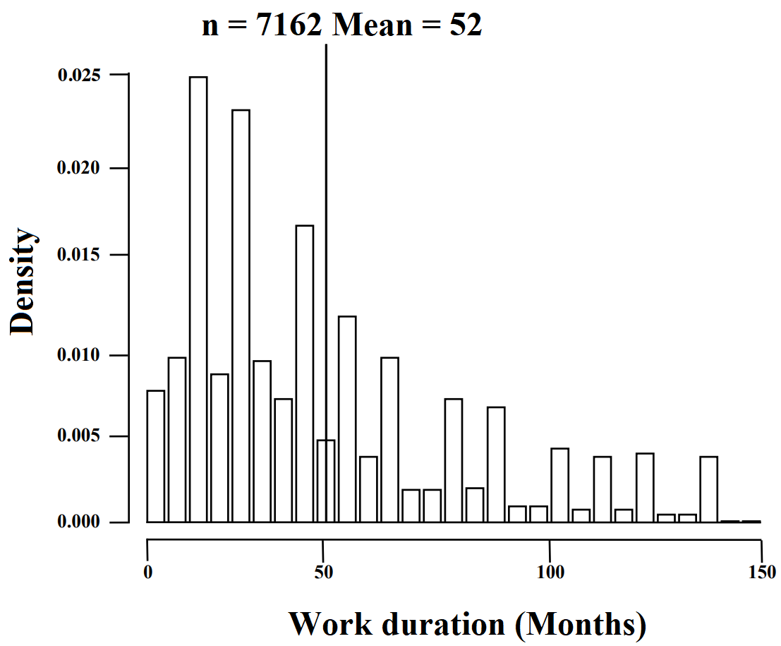
Figure 13. Work duration histograms on particular projects; from (Sela and Ben-Gal, 2018). Data from: Facebook, eBay, Apple, 3M, Intel, and Motorola.

All these problems with trust, insight, training, and tool development can be solved if, early on in the project, a software defect prediction model can be learned that is effective for the rest of the life cycle (which is the main result of this paper). Within that data, we have found that models learned after just 150 commits, perform just as well as anything else. In terms of resolving conclusion instability, this is a very significant result since it means that for much of the life cycle, we can offer stable defect predictors.

One way to consider the impact of such early life cycle predictors is to use the data of Figure 13. That plot shows that software employees usually change projects every 52 months (either moving between companies or changing projects within an organization). According to Figure 13, in seven years (84 months), the majority of workers and managers would first appear on a job after the initial four months are required to learn a defect predictor. Hence, for most workers and managers, the detectors learned via the methods of this paper would be the “established wisdom” and “the way we do things here” for their projects. This means that a detector learned in the first four months would be a suitable oracle to guide training and hiring; the development of code review practices; the automation of local “bad smell detectors”; as well as tool selection and development.

8.2. Systems Implications

Figure 9 shows the run-time required to find bellwether projects in all 240 projects using $\mathit{Bellwether}$ or $\mathit{E_{size}(Bellwether)}$ policies. Note that the early-bird methods use 2.5 months less CPU than the alternative.

Since we only need the first 150 commits to identify a suitable project, many projects in their early stages may be included in the pool of transferable projects. Importantly Figure 8 show when sampled using $\mathit{E_{size}}$ 30% “more projects” were qualified in much “less time”. The choice of bellwether does not matter; perhaps, in practice, practitioners need not continue to look for bellwethers and terminate early as soon as they find the first bellwether. This could also mean lesser privacy concerns and enable practitioners to share fewer data freely. The early-data nature of our methods can also help to gauge sophisticated techniques like TCA+ faster.

Note: We do not claim $E_{size}(Bellwether)$ is data-lite because it would still process all the projects in the search space. But we do endorse $E_{size}$ over current methods $Bellwether$ or $TCA+$. Because $E_{size}$ uses fixed data (150 commits) and does not re-train for every new project release it is faster and more accurate (see §6.3).

Practitioners may feel that retraining defect prediction models for every project release may not be a tedious activity. However, our prior work (Shrikanth et al., 2021) points out two concerns. First, models that are frequently retrained may yield different conclusions. As seen from Figure 1 information is rich in the earlier periods of the project. When including training data from uninformative regions (training with recent releases or all available data) the model would yield different conclusions. In other words, a commit that was classified as defective could be classified as clean in another project release causing confusion within teams. Second, it is a methodological error to learn (sample training data) from the shallow end of the project region.

8.3. Research Implications

We have shown that when defect data contains information, that information may be densest in a small part of the historical record of a project. While we have not shown that other kinds of SE data have the same density effect, we would argue that now it is at least an open question that “have we been learning from the wrong parts of the data?”.

Finally, we should now view it as a potential methodological error to reason across all data in a project. In the specific case of software defect prediction we must now revisit any conclusion based just on later life cycle data There are many examples of such conclusions. For example:

• Hoang et al. says “We assume that older commits changes may have characteristics that no longer effects to the latest commits” (Hoang et al., 2019).

• Also, it is common practice in software defect prediction to perform “recent validation” where predictors are tested on the latest release after training from the prior one or two releases (Tan et al., 2015; McIntosh and Kamei, 2017; Kondo et al., 2020; Fu et al., 2016).

More generally, before researchers focus on later life cycle data, they must first check that their buggy commit data occur at equal frequency across the life cycle. If the buggy commits data is isolated to a specific region, then predictors should be built from that region. This work finds that most buggy commits are found early in the project life cycle.

9. Conclusion

Issues with conclusion instability, run-time complexity, and explanations of models improve if we can learn a predictive model early in the life cycle that is effective for the rest of the project. The prior work on software defect prediction identified the “early bird” heuristic. However, the results were scoped only in the context of within-project defect prediction on popular GitHub projects (Shrikanth et al., 2021).

We expanded the scope of the early method to simplify software defect prediction. Specifically, the results of this work find that a small early life cycle sample with two features can replace some methods and usefully augment others. For within-project defect prediction, when trying to improve predictive performance, the extra CPU required for (a) ensemble and (b) hyper-parameter optimization is not needed since sampling from early life cycle data performs better than both (a) and (b). As to transfer learning in cross-company learning, this work recommends that a small early life cycle sample on cross-project learning is significantly better than using the entire cross-project life cycle data.

As for future work, perhaps we can simplify many SE tasks using the “early bird” heuristic.

References

- (1)
- Aggarwal et al. (2001) Charu C. Aggarwal, Alexander Hinneburg, and Daniel A. Keim. 2001. On the Surprising Behavior of Distance Metrics in High Dimensional Spaces. In Proceedings of the 8th International Conference on Database Theory (ICDT ’01). Springer-Verlag, Berlin, Heidelberg, 420–434.
- Agrawal et al. (2019) Amritanshu Agrawal, Wei Fu, Di Chen, Xipeng Shen, and Tim Menzies. 2019. How to”” DODGE”” Complex Software Analytics. IEEE Transactions on Software Engineering (2019).
- Agrawal et al. (2018) Amritanshu Agrawal, Wei Fu, and Tim Menzies. 2018. What is wrong with topic modeling? And how to fix it using search-based software engineering. Information and Software Technology 98 (2018), 74–88.
- Agrawal and Menzies (2018) Amritanshu Agrawal and Tim Menzies. 2018. Is”” Better Data”” Better Than”” Better Data Miners””?. In 2018 IEEE/ACM 40th International Conference on Software Engineering (ICSE). IEEE, 1050–1061.
- Agrawal et al. (2021) Amritanshu Agrawal, Xueqi Yang, Rishabh Agrawal, Rahul Yedida, Xipeng Shen, and Tim Menzies. 2021. Simpler Hyperparameter Optimization for Software Analytics: Why, How, When. IEEE Transactions on Software Engineering (2021).
- Akiyama (1971) Fumio Akiyama. 1971. An Example of Software System Debugging.. In IFIP Congress (1), Vol. 71. 353–359.
- Amasaki (2020) Sousuke Amasaki. 2020. Cross-version defect prediction: use historical data, cross-project data, or both? Empirical Software Engineering (2020), 1–23.
- Arokiam and Bradbury (2020) J. Arokiam and J. Bradbury. 2020. Automatically Predicting Bug Severity Early in the Development Process. In 2020 42nd International Conference on Software Engineering (ICSE).
- Bennin et al. (2019) Kwabena Ebo Bennin, Jacky W Keung, and Akito Monden. 2019. On the relative value of data resampling approaches for software defect prediction. Empirical Software Engineering 24, 2 (2019), 602–636.
- Bergstra et al. (2011) James Bergstra, Rémi Bardenet, Yoshua Bengio, and Balázs Kégl. 2011. Algorithms for Hyper-parameter Optimization. In Proceedings of the 24th International Conference on Neural Information Processing Systems (Granada, Spain) (NIPS’11). Curran Associates Inc., USA, 2546–2554. http://dl.acm.org/citation.cfm?id=2986459.2986743
- Bergstra et al. (2013) James Bergstra, Daniel Yamins, and David Cox. 2013. Making a science of model search: Hyperparameter optimization in hundreds of dimensions for vision architectures. In International conference on machine learning. PMLR, 115–123.
- Bettenburg et al. (2012) Nicolas Bettenburg, Meiyappan Nagappan, and Ahmed E Hassan. 2012. Think locally, act globally: Improving defect and effort prediction models. In 2012 9th IEEE Working Conference on Mining Software Repositories (MSR). IEEE, 60–69.
- Bird et al. (2015) Christian Bird, Tim Menzies, and Thomas Zimmermann. 2015. The Art and Science of Analyzing Software Data (1st ed.). Morgan Kaufmann Publishers Inc., San Francisco, CA, USA.
- Bird et al. (2011) Christian Bird, Nachiappan Nagappan, Brendan Murphy, Harald Gall, and Premkumar Devanbu. 2011. Don’t touch my code! Examining the effects of ownership on software quality. In Proceedings of the 19th ACM SIGSOFT symposium and the 13th European conference on Foundations of software engineering. 4–14.
- Boehm et al. (2005) Barry Boehm, Ricardo Valerdi, J Lane, and AW Brown. 2005. COCOMO suite methodology and evolution. CrossTalk 18, 4 (2005), 20–25.
- Bowes et al. (2018) David Bowes, Tracy Hall, and Jean Petrić. 2018. Software defect prediction: do different classifiers find the same defects? Software Quality Journal 26, 2 (2018), 525–552.
- Briand et al. (2002) Lionel C Briand, Walcelio L. Melo, and Jurgen Wust. 2002. Assessing the applicability of fault-proneness models across object-oriented software projects. IEEE transactions on Software Engineering 28, 7 (2002), 706–720.
- Canfora et al. (2013) Gerardo Canfora, Andrea De Lucia, Massimiliano Di Penta, Rocco Oliveto, Annibale Panichella, and Sebastiano Panichella. 2013. Multi-objective cross-project defect prediction. In 2013 IEEE Sixth International Conference on Software Testing, Verification and Validation. IEEE, 252–261.
- Canfora et al. (2015) Gerardo Canfora, Andrea De Lucia, Massimiliano Di Penta, Rocco Oliveto, Annibale Panichella, and Sebastiano Panichella. 2015. Defect prediction as a multiobjective optimization problem. Software Testing, Verification and Reliability 25, 4 (2015), 426–459.
- Chawla et al. (2002) Nitesh V Chawla, Kevin W Bowyer, Lawrence O Hall, and W Philip Kegelmeyer. 2002. SMOTE: synthetic minority over-sampling technique. Journal of artificial intelligence research 16 (2002), 321–357.
- Chekam et al. (2020) Thierry Titcheu Chekam, Mike Papadakis, Tegawendé F Bissyandé, Yves Le Traon, and Koushik Sen. 2020. Selecting fault revealing mutants. Empirical Software Engineering 25, 1 (2020), 434–487.
- Chen et al. (2018a) Di Chen, Wei Fu, Rahul Krishna, and Tim Menzies. 2018a. Applications of psychological science for actionable analytics. FSE’19 (2018).
- Chen et al. (2019a) Jinyin Chen, Yitao Yang, Keke Hu, Qi Xuan, Yi Liu, and Chao Yang. 2019a. Multiview transfer learning for software defect prediction. IEEE Access 7 (2019), 8901–8916.
- Chen et al. (2015) Lin Chen, Bin Fang, Zhaowei Shang, and Yuanyan Tang. 2015. Negative samples reduction in cross-company software defects prediction. Information and Software Technology 62 (2015), 67–77.
- Chen et al. (2019b) Xiang Chen, Dun Zhang, Yingquan Zhao, Zhanqi Cui, and Chao Ni. 2019b. Software defect number prediction: Unsupervised vs supervised methods. Information and Software Technology 106 (2019), 161–181.
- Chen et al. (2018b) Xiang Chen, Yingquan Zhao, Qiuping Wang, and Zhidan Yuan. 2018b. MULTI: Multi-objective effort-aware just-in-time software defect prediction. Information and Software Technology 93 (2018), 1–13.
- Dam et al. (2018) Hoa Khanh Dam, Trang Pham, Shien Wee Ng, Truyen Tran, John Grundy, Aditya Ghose, Taeksu Kim, and Chul-Joo Kim. 2018. A deep tree-based model for software defect prediction. arXiv preprint arXiv:1802.00921 (2018).
- D’Ambros et al. (2012) Marco D’Ambros, Michele Lanza, and Romain Robbes. 2012. Evaluating defect prediction approaches: a benchmark and an extensive comparison. Empirical Software Engineering 17, 4-5 (2012), 531–577.
- Fenton et al. (2008) Norman Fenton, Martin Neil, William Marsh, Peter Hearty, Łukasz Radliński, and Paul Krause. 2008. On the effectiveness of early life cycle defect prediction with Bayesian Nets. Empirical Software Engineering 13, 5 (2008), 499.
- Fu et al. (2016) Wei Fu, Tim Menzies, and Xipeng Shen. 2016. Tuning for software analytics: Is it really necessary? Information and Software Technology 76 (2016), 135–146.
- Fukushima et al. (2014) Takafumi Fukushima, Yasutaka Kamei, Shane McIntosh, Kazuhiro Yamashita, and Naoyasu Ubayashi. 2014. An empirical study of just-in-time defect prediction using cross-project models. In Proceedings of the 11th Working Conference on Mining Software Repositories. 172–181.
- Ghotra et al. (2015) Baljinder Ghotra, Shane McIntosh, and Ahmed E Hassan. 2015. Revisiting the impact of classification techniques on the performance of defect prediction models. In 2015 IEEE/ACM 37th IEEE International Conference on Software Engineering, Vol. 1. IEEE, 789–800.
- Hailpern and Santhanam (2002) Brent Hailpern and Padmanabhan Santhanam. 2002. Software debugging, testing, and verification. IBM Systems Journal 41, 1 (2002), 4–12.
- Hall and Holmes (2003) Mark A Hall and Geoffrey Holmes. 2003. Benchmarking attribute selection techniques for discrete class data mining. IEEE Transactions on Knowledge and Data engineering 15, 6 (2003), 1437–1447.
- Hassan (2017) A. Hassan. 2017. Remarks made during a presentation to the UCL Crest Open Workshop.
- He and Garcia (2009) Haibo He and Edwardo A Garcia. 2009. Learning from imbalanced data. IEEE Transactions on knowledge and data engineering 21, 9 (2009), 1263–1284.
- He et al. (2015) Peng He, Bing Li, Xiao Liu, Jun Chen, and Yutao Ma. 2015. An empirical study on software defect prediction with a simplified metric set. Information and Software Technology 59 (2015), 170–190.
- He et al. (2013) Zhimin He, Fayola Peters, Tim Menzies, and Ye Yang. 2013. Learning from open-source projects: An empirical study on defect prediction. In 2013 ACM/IEEE international symposium on empirical software engineering and measurement. IEEE, 45–54.
- He et al. (2012) Zhimin He, Fengdi Shu, Ye Yang, Mingshu Li, and Qing Wang. 2012. An investigation on the feasibility of cross-project defect prediction. Automated Software Engineering 19, 2 (2012), 167–199.
- Herbold (2013) Steffen Herbold. 2013. Training data selection for cross-project defect prediction. In Proceedings of the 9th international conference on predictive models in software engineering. 1–10.
- Hoang et al. (2019) T. Hoang, H. Khanh Dam, Y. Kamei, D. Lo, and N. Ubayashi. 2019. DeepJIT: An End-to-End Deep Learning Framework for Just-in-Time Defect Prediction. In 2019 IEEE/ACM 16th International Conference on Mining Software Repositories (MSR). 34–45.
- Hosseini et al. (2018) Seyedrebvar Hosseini, Burak Turhan, and Mika M”̈antyl”̈a. 2018. A benchmark study on the effectiveness of search-based data selection and feature selection for cross project defect prediction. Information and Software Technology 95 (2018), 296–312.
- Huang et al. (2019) Qiao Huang, Xin Xia, and David Lo. 2019. Revisiting supervised and unsupervised models for effort-aware just-in-time defect prediction. Empirical Software Engineering 24, 5 (2019), 2823–2862.
- Huda et al. (2018) Shamsul Huda, Kevin Liu, Mohamed Abdelrazek, Amani Ibrahim, Sultan Alyahya, Hmood Al-Dossari, and Shafiq Ahmad. 2018. An ensemble oversampling model for class imbalance problem in software defect prediction. IEEE access 6 (2018), 24184–24195.
- Jiang et al. (2013) Tian Jiang, Lin Tan, and Sunghun Kim. 2013. Personalized defect prediction. In 2013 28th IEEE/ACM International Conference on Automated Software Engineering (ASE). Ieee, 279–289.
- Jing et al. (2015) Xiaoyuan Jing, Fei Wu, Xiwei Dong, Fumin Qi, and Baowen Xu. 2015. Heterogeneous cross-company defect prediction by unified metric representation and CCA-based transfer learning. In Proceedings of the 2015 10th Joint Meeting on Foundations of Software Engineering. 496–507.
- Jing et al. (2016) Xiao-Yuan Jing, Fei Wu, Xiwei Dong, and Baowen Xu. 2016. An improved SDA based defect prediction framework for both within-project and cross-project class-imbalance problems. IEEE Transactions on Software Engineering 43, 4 (2016), 321–339.
- Kamei et al. (2016) Yasutaka Kamei, Takafumi Fukushima, Shane McIntosh, Kazuhiro Yamashita, Naoyasu Ubayashi, and Ahmed E Hassan. 2016. Studying just-in-time defect prediction using cross-project models. Empirical Software Engineering 21, 5 (2016), 2072–2106.
- Kamei et al. (2012) Yasutaka Kamei, Emad Shihab, Bram Adams, Ahmed E Hassan, Audris Mockus, Anand Sinha, and Naoyasu Ubayashi. 2012. A large-scale empirical study of just-in-time quality assurance. IEEE Transactions on Software Engineering 39, 6 (2012), 757–773.
- Kim et al. (2011) Miryung Kim, Dongxiang Cai, and Sunghun Kim. 2011. An empirical investigation into the role of API-level refactorings during software evolution. In Proceedings of the 33rd International Conference on Software Engineering. ACM, 151–160.
- Kim et al. (2016) Miryung Kim, Thomas Zimmermann, Robert DeLine, and Andrew Begel. 2016. The Emerging Role of Data Scientists on Software Development Teams. In Proceedings of the 38th International Conference on Software Engineering (Austin, Texas) (ICSE ’16). ACM, New York, NY, USA, 96–107. https://doi.org/10.1145/2884781.2884783
- Kocaguneli et al. (2015) Ekrem Kocaguneli, Tim Menzies, and Emilia Mendes. 2015. Transfer learning in effort estimation. Empirical Software Engineering 20, 3 (June 2015), 813–843. https://doi.org/10.1007/s10664-014-9300-5
- Kondo et al. (2019) Masanari Kondo, Cor-Paul Bezemer, Yasutaka Kamei, Ahmed E Hassan, and Osamu Mizuno. 2019. The impact of feature reduction techniques on defect prediction models. Empirical Software Engineering 24, 4 (2019), 1925–1963.
- Kondo et al. (2020) Masanari Kondo, Daniel M German, Osamu Mizuno, and Eun-Hye Choi. 2020. The impact of context metrics on just-in-time defect prediction. Empirical Software Engineering 25, 1 (2020), 890–939.
- Koru et al. (2008a) A Güneş Koru, Khaled El Emam, Dongsong Zhang, Hongfang Liu, and Divya Mathew. 2008a. Theory of relative defect proneness. Empirical Software Engineering 13, 5 (2008), 473–498.
- Koru et al. (2008b) A Güneş Koru, Dongsong Zhang, Khaled El Emam, and Hongfang Liu. 2008b. An investigation into the functional form of the size-defect relationship for software modules. IEEE Transactions on Software Engineering 35, 2 (2008), 293–304.
- Krishna and Menzies (2018) Rahul Krishna and Tim Menzies. 2018. Bellwethers: A baseline method for transfer learning. IEEE Transactions on Software Engineering 45, 11 (2018), 1081–1105.
- Krishna et al. (2016) Rahul Krishna, Tim Menzies, and Wei Fu. 2016. Too much automation? The bellwether effect and its implications for transfer learning. In Proceedings of the 31st IEEE/ACM International Conference on Automated Software Engineering. 122–131.
- Lam et al. (2017) An Ngoc Lam, Anh Tuan Nguyen, Hoan Anh Nguyen, and Tien N Nguyen. 2017. Bug localization with combination of deep learning and information retrieval. In 2017 IEEE/ACM 25th International Conference on Program Comprehension (ICPC). IEEE, 218–229.
- Laradji et al. (2015) Issam H Laradji, Mohammad Alshayeb, and Lahouari Ghouti. 2015. Software defect prediction using ensemble learning on selected features. Information and Software Technology 58 (2015), 388–402.
- Levina and Bickel (2005) Elizaveta Levina and Peter J Bickel. 2005. Maximum likelihood estimation of intrinsic dimension. In Advances in neural information processing systems. 777–784.
- Li et al. (2017) Jian Li, Pinjia He, Jieming Zhu, and Michael R Lyu. 2017. Software defect prediction via convolutional neural network. In 2017 IEEE International Conference on Software Quality, Reliability and Security (QRS). IEEE, 318–328.
- Li et al. (2012) Ming Li, Hongyu Zhang, Rongxin Wu, and Zhi-Hua Zhou. 2012. Sample-based software defect prediction with active and semi-supervised learning. Automated Software Engineering 19, 2 (2012), 201–230.
- Li et al. (2018) Zhiqiang Li, Xiao-Yuan Jing, Fei Wu, Xiaoke Zhu, Baowen Xu, and Shi Ying. 2018. Cost-sensitive transfer kernel canonical correlation analysis for heterogeneous defect prediction. Automated Software Engineering 25, 2 (2018), 201–245.
- Liu et al. (2019) Chao Liu, Dan Yang, Xin Xia, Meng Yan, and Xiaohong Zhang. 2019. A two-phase transfer learning model for cross-project defect prediction. Information and Software Technology 107 (2019), 125–136.
- Ma et al. (2012) Ying Ma, Guangchun Luo, Xue Zeng, and Aiguo Chen. 2012. Transfer learning for cross-company software defect prediction. Information and Software Technology 54, 3 (2012), 248–256.
- Mathew et al. (2018) George Mathew, Amritanshu Agrawal, and Tim Menzies. 2018. Finding trends in software research. IEEE Transactions on Software Engineering (2018).
- McIntosh and Kamei (2017) Shane McIntosh and Yasutaka Kamei. 2017. Are fix-inducing changes a moving target? a longitudinal case study of just-in-time defect prediction. IEEE Transactions on Software Engineering 44, 5 (2017), 412–428.
- Menzies et al. (2012) Tim Menzies, Andrew Butcher, David Cok, Andrian Marcus, Lucas Layman, Forrest Shull, Burak Turhan, and Thomas Zimmermann. 2012. Local versus global lessons for defect prediction and effort estimation. IEEE Transactions on software engineering 39, 6 (2012), 822–834.
- Menzies et al. (2011) Tim Menzies, Andrew Butcher, Andrian Marcus, Thomas Zimmermann, and David Cok. 2011. Local vs. global models for effort estimation and defect prediction. In 2011 26th IEEE/ACM International Conference on Automated Software Engineering (ASE 2011). IEEE, 343–351.
- Menzies et al. (2006) Tim Menzies, Jeremy Greenwald, and Art Frank. 2006. Data mining static code attributes to learn defect predictors. IEEE transactions on software engineering 33, 1 (2006), 2–13.
- Menzies et al. (2010) Tim Menzies, Zach Milton, Burak Turhan, Bojan Cukic, Yue Jiang, and Ayşe Bener. 2010. Defect prediction from static code features: current results, limitations, new approaches. Automated Software Engineering 17, 4 (2010), 375–407.
- Menzies et al. (2008) Tim Menzies, Burak Turhan, Ayse Bener, Gregory Gay, Bojan Cukic, and Yue Jiang. 2008. Implications of ceiling effects in defect predictors. In Proceedings of the 4th international workshop on Predictor models in software engineering. 47–54.
- Misirli et al. (2011) Ayse Tosun Misirli, Ayse Bener, and Resat Kale. 2011. Ai-based software defect predictors: Applications and benefits in a case study. AI Magazine 32, 2 (2011), 57–68.
- Mittas and Angelis (2013) N. Mittas and L. Angelis. 2013. Ranking and Clustering Software Cost Estimation Models through a Multiple Comparisons Algorithm. IEEE Trans SE 39, 4 (April 2013), 537–551. https://doi.org/10.1109/TSE.2012.45
- Munaiah et al. (2017) Nuthan Munaiah, Steven Kroh, Craig Cabrey, and Meiyappan Nagappan. 2017. Curating GitHub for engineered software projects. Empirical Software Engineering 22, 6 (2017), 3219–3253.
- Nagappan and Ball (2005) Nachiappan Nagappan and Thomas Ball. 2005. Use of relative code churn measures to predict system defect density. In Proceedings of the 27th international conference on Software engineering. ACM, 284–292.
- Nam et al. (2017) Jaechang Nam, Wei Fu, Sunghun Kim, Tim Menzies, and Lin Tan. 2017. Heterogeneous defect prediction. IEEE Transactions on Software Engineering 44, 9 (2017), 874–896.
- Nam et al. (2013a) Jaechang Nam, Sinno Jialin Pan, and Sunghun Kim. 2013a. Transfer defect learning. In 2013 35th international conference on software engineering (ICSE). IEEE, 382–391.
- Nam et al. (2013b) Jaechang Nam, Sinno Jialin Pan, and Sunghun Kim. 2013b. Transfer defect learning. In Proceedings - International Conference on Software Engineering. 382–391. https://doi.org/10.1109/ICSE.2013.6606584
- Ni et al. (2017) Chao Ni, Wang-Shu Liu, Xiang Chen, Qing Gu, Dao-Xu Chen, and Qi-Guo Huang. 2017. A cluster based feature selection method for cross-project software defect prediction. Journal of Computer Science and Technology 32, 6 (2017), 1090–1107.
- Ostrand et al. (2005) Thomas J Ostrand, Elaine J Weyuker, and Robert M Bell. 2005. Predicting the location and number of faults in large software systems. IEEE Transactions on Software Engineering 31, 4 (2005), 340–355.
- Pan et al. (2010) Sinno Jialin Pan, Ivor W Tsang, James T Kwok, and Qiang Yang. 2010. Domain adaptation via transfer component analysis. IEEE Transactions on Neural Networks 22, 2 (2010), 199–210.
- Pandey et al. (2020) Sushant Kumar Pandey, Ravi Bhushan Mishra, and Anil Kumar Tripathi. 2020. BPDET: An effective software bug prediction model using deep representation and ensemble learning techniques. Expert Systems with Applications 144 (2020), 113085.
- Panichella et al. (2014) Annibale Panichella, Rocco Oliveto, and Andrea De Lucia. 2014. Cross-project defect prediction models: L’union fait la force. In 2014 Software Evolution Week-IEEE Conference on Software Maintenance, Reengineering, and Reverse Engineering (CSMR-WCRE). IEEE, 164–173.
- Parnin and Orso (2011) Chris Parnin and Alessandro Orso. 2011. Are automated debugging techniques actually helping programmers?. In Proceedings of the 2011 international symposium on software testing and analysis. ACM, 199–209.
- Pascarella et al. (2019) Luca Pascarella, Fabio Palomba, and Alberto Bacchelli. 2019. Fine-grained just-in-time defect prediction. Journal of Systems and Software 150 (2019), 22–36.
- Pedregosa et al. (2011a) Fabian Pedregosa, Gaël Varoquaux, Alexandre Gramfort, Vincent Michel, Bertrand Thirion, Olivier Grisel, Mathieu Blondel, Peter Prettenhofer, Ron Weiss, Vincent Dubourg, et al. 2011a. Scikit-learn: Machine learning in Python. the Journal of machine Learning research 12 (2011), 2825–2830.
- Pedregosa et al. (2011b) F. Pedregosa, G. Varoquaux, A. Gramfort, V. Michel, B. Thirion, O. Grisel, M. Blondel, P. Prettenhofer, R. Weiss, V. Dubourg, J. Vanderplas, A. Passos, D. Cournapeau, M. Brucher, M. Perrot, and E. Duchesnay. 2011b. Scikit-learn: Machine Learning in Python. Journal of Machine Learning Research 12 (2011), 2825–2830.
- Peters et al. (2013b) Fayola Peters, Tim Menzies, Liang Gong, and Hongyu Zhang. 2013b. Balancing privacy and utility in cross-company defect prediction. IEEE Transactions on Software Engineering 39, 8 (2013), 1054–1068.
- Peters et al. (2015) Fayola Peters, Tim Menzies, and Lucas Layman. 2015. LACE2: Better privacy-preserving data sharing for cross project defect prediction. In 2015 IEEE/ACM 37th IEEE International Conference on Software Engineering, Vol. 1. IEEE, 801–811.
- Peters et al. (2013a) Fayola Peters, Tim Menzies, and Andrian Marcus. 2013a. Better cross company defect prediction. In 2013 10th Working Conference on Mining Software Repositories (MSR). IEEE, 409–418.
- Rahman and Devanbu (2013) Foyzur Rahman and Premkumar Devanbu. 2013. How, and why, process metrics are better. In 2013 35th International Conference on Software Engineering (ICSE). IEEE, 432–441.
- Rahman et al. (2014) Foyzur Rahman, Sameer Khatri, Earl T. Barr, and Premkumar Devanbu. 2014. Comparing Static Bug Finders and Statistical Prediction. In Proceedings of the 36th International Conference on Software Engineering (Hyderabad, India) (ICSE 2014). Association for Computing Machinery, New York, NY, USA, 424–434. https://doi.org/10.1145/2568225.2568269
- Rahman et al. (2012) Foyzur Rahman, Daryl Posnett, and Premkumar Devanbu. 2012. Recalling the”” imprecision”” of cross-project defect prediction. In Proceedings of the ACM SIGSOFT 20th International Symposium on the Foundations of Software Engineering. 1–11.
- Rahman et al. (2013) Foyzur Rahman, Daryl Posnett, Israel Herraiz, and Premkumar Devanbu. 2013. Sample size vs. bias in defect prediction. In Proceedings of the 2013 9th joint meeting on foundations of software engineering. ACM, 147–157.
- Rathore and Kumar (2017) Santosh Singh Rathore and Sandeep Kumar. 2017. Towards an ensemble based system for predicting the number of software faults. Expert Systems with Applications 82 (2017), 357–382.
- Rhmann et al. (2020) Wasiur Rhmann, Babita Pandey, Gufran Ansari, and Devendra Kumar Pandey. 2020. Software fault prediction based on change metrics using hybrid algorithms: An empirical study. Journal of King Saud University-Computer and Information Sciences 32, 4 (2020), 419–424.
- Rosen et al. (2015) Christoffer Rosen, Ben Grawi, and Emad Shihab. 2015. Commit guru: analytics and risk prediction of software commits. In Proceedings of the 2015 10th Joint Meeting on Foundations of Software Engineering. ACM, 966–969.
- Ryu and Baik (2016) Duksan Ryu and Jongmoon Baik. 2016. Effective multi-objective na”̈ıve Bayes learning for cross-project defect prediction. Applied Soft Computing 49 (2016), 1062–1077.
- Ryu et al. (2016) Duksan Ryu, Okjoo Choi, and Jongmoon Baik. 2016. Value-cognitive boosting with a support vector machine for cross-project defect prediction. Empirical Software Engineering 21, 1 (2016), 43–71.
- Ryu et al. (2015) Duksan Ryu, Jong-In Jang, and Jongmoon Baik. 2015. A hybrid instance selection using nearest-neighbor for cross-project defect prediction. Journal of Computer Science and Technology 30, 5 (2015), 969–980.
- Ryu et al. (2017) Duksan Ryu, Jong-In Jang, and Jongmoon Baik. 2017. A transfer cost-sensitive boosting approach for cross-project defect prediction. Software Quality Journal 25, 1 (2017), 235–272.
- Sawyer (2013) Robert Sawyer. 2013. BI’s Impact on Analyses and Decision Making Depends on the Development of Less Complex Applications. In Principles and Applications of Business Intelligence Research. IGI Global, 83–95.
- Scandariato et al. (2014) Riccardo Scandariato, James Walden, Aram Hovsepyan, and Wouter Joosen. 2014. Predicting vulnerable software components via text mining. IEEE Transactions on Software Engineering 40, 10 (2014), 993–1006.
- Sela and Ben-Gal (2018) Alon Sela and Hila Chalutz Ben-Gal. 2018. Big data analysis of employee turnover in global media companies, google, facebook and others. In 2018 IEEE International Conference on the Science of Electrical Engineering in Israel (ICSEE). IEEE, 1–5.
- Shihab et al. (2010) Emad Shihab, Zhen Ming Jiang, Walid M Ibrahim, Bram Adams, and Ahmed E Hassan. 2010. Understanding the impact of code and process metrics on post-release defects: a case study on the eclipse project. In Proceedings of the 2010 ACM-IEEE International Symposium on Empirical Software Engineering and Measurement. 1–10.
- Shrikanth et al. (2021) N. Shrikanth, S. Majumder, and T. Menzies. 2021. Early Life Cycle Software Defect Prediction. Why? How?. In 2021 IEEE/ACM 43rd International Conference on Software Engineering (ICSE). IEEE Computer Society, Los Alamitos, CA, USA, 448–459. https://doi.org/10.1109/ICSE43902.2021.00050
- Shrikanth and Menzies (2020) NC Shrikanth and Tim Menzies. 2020. Assessing practitioner beliefs about software defect prediction. In 2020 IEEE/ACM 42nd International Conference on Software Engineering: Software Engineering in Practice (ICSE-SEIP). IEEE, 182–190.
- Siers and Islam (2015) Michael J Siers and Md Zahidul Islam. 2015. Software defect prediction using a cost sensitive decision forest and voting, and a potential solution to the class imbalance problem. Information Systems 51 (2015), 62–71.
- Śliwerski et al. (2005) Jacek Śliwerski, Thomas Zimmermann, and Andreas Zeller. 2005. When Do Changes Induce Fixes?. In Proceedings of the 2005 International Workshop on Mining Software Repositories (St. Louis, Missouri) (MSR ’05). ACM, New York, NY, USA, 1–5. https://doi.org/10.1145/1082983.1083147
- Song et al. (2018) Qinbao Song, Yuchen Guo, and Martin Shepperd. 2018. A comprehensive investigation of the role of imbalanced learning for software defect prediction. IEEE Transactions on Software Engineering 45, 12 (2018), 1253–1269.
- Sun et al. (2012) Zhongbin Sun, Qinbao Song, and Xiaoyan Zhu. 2012. Using coding-based ensemble learning to improve software defect prediction. IEEE Transactions on Systems, Man, and Cybernetics, Part C (Applications and Reviews) 42, 6 (2012), 1806–1817.
- Tan et al. (2015) Ming Tan, Lin Tan, Sashank Dara, and Caleb Mayeux. 2015. Online defect prediction for imbalanced data. In 2015 IEEE/ACM 37th IEEE International Conference on Software Engineering, Vol. 2. IEEE, 99–108.
- Tan and Chan (2016) Shiang-Yen Tan and Taizan Chan. 2016. Defining and conceptualizing actionable insight: a conceptual framework for decision-centric analytics. arXiv preprint arXiv:1606.03510 (2016).
- Tantithamthavorn et al. (2018) C. Tantithamthavorn, A. E. Hassan, and K. Matsumoto. 2018. The Impact of Class Rebalancing Techniques on the Performance and Interpretation of Defect Prediction Models. IEEE Transactions on Software Engineering (2018), 1–1.
- Tantithamthavorn et al. (2016) Chakkrit Tantithamthavorn, Shane McIntosh, Ahmed E Hassan, and Kenichi Matsumoto. 2016. Automated parameter optimization of classification techniques for defect prediction models. In Proceedings of the 38th International Conference on Software Engineering. 321–332.
- Tantithamthavorn et al. (2018) Chakkrit Tantithamthavorn, Shane McIntosh, Ahmed E Hassan, and Kenichi Matsumoto. 2018. The impact of automated parameter optimization on defect prediction models. IEEE Transactions on Software Engineering 45, 7 (2018), 683–711.
- Tong et al. (2018) Haonan Tong, Bin Liu, and Shihai Wang. 2018. Software defect prediction using stacked denoising autoencoders and two-stage ensemble learning. Information and Software Technology 96 (2018), 94–111.
- Turhan et al. (2013) Burak Turhan, Ayşe Tosun Mısırlı, and Ayşe Bener. 2013. Empirical evaluation of the effects of mixed project data on learning defect predictors. Information and Software Technology 55, 6 (2013), 1101–1118.
- Vargha and Delaney (2000) András Vargha and Harold D Delaney. 2000. A critique and improvement of the CL common language effect size statistics of McGraw and Wong. Journal of Educational and Behavioral Statistics 25, 2 (2000), 101–132.
- Wan et al. (2018) Zhiyuan Wan, Xin Xia, Ahmed E Hassan, David Lo, Jianwei Yin, and Xiaohu Yang. 2018. Perceptions, expectations, and challenges in defect prediction. IEEE Transactions on Software Engineering (2018).
- Wang et al. (2018) Song Wang, Taiyue Liu, Jaechang Nam, and Lin Tan. 2018. Deep semantic feature learning for software defect prediction. IEEE Transactions on Software Engineering (2018).
- Wang et al. (2016a) Song Wang, Taiyue Liu, and Lin Tan. 2016a. Automatically learning semantic features for defect prediction. In 2016 IEEE/ACM 38th International Conference on Software Engineering (ICSE). IEEE, 297–308.
- Wang and Yao (2013) Shuo Wang and Xin Yao. 2013. Using class imbalance learning for software defect prediction. IEEE Transactions on Reliability 62, 2 (2013), 434–443.
- Wang et al. (2016b) Tiejian Wang, Zhiwu Zhang, Xiaoyuan Jing, and Liqiang Zhang. 2016b. Multiple kernel ensemble learning for software defect prediction. Automated Software Engineering 23, 4 (2016), 569–590.
- Weyuker et al. (2008) Elaine J Weyuker, Thomas J Ostrand, and Robert M Bell. 2008. Do too many cooks spoil the broth? using the number of developers to enhance defect prediction models. Empirical Software Engineering 13, 5 (2008), 539–559.
- Wu et al. (2018) Fei Wu, Xiao-Yuan Jing, Ying Sun, Jing Sun, Lin Huang, Fangyi Cui, and Yanfei Sun. 2018. Cross-project and within-project semisupervised software defect prediction: A unified approach. IEEE Transactions on Reliability 67, 2 (2018), 581–597.
- Xia et al. (2016a) Xin Xia, David Lo, Sinno Jialin Pan, Nachiappan Nagappan, and Xinyu Wang. 2016a. Hydra: Massively compositional model for cross-project defect prediction. IEEE Transactions on software Engineering 42, 10 (2016), 977–998.
- Xia et al. (2016b) Xin Xia, Emad Shihab, Yasutaka Kamei, David Lo, and Xinyu Wang. 2016b. Predicting crashing releases of mobile applications. In Proceedings of the 10th ACM/IEEE International Symposium on Empirical Software Engineering and Measurement. 1–10.
- Xu et al. (2019) Zhou Xu, Jin Liu, Xiapu Luo, Zijiang Yang, Yifeng Zhang, Peipei Yuan, Yutian Tang, and Tao Zhang. 2019. Software defect prediction based on kernel PCA and weighted extreme learning machine. Information and Software Technology 106 (2019), 182–200.
- Yan et al. (2020) Meng Yan, Xin Xia, Yuanrui Fan, Ahmed E Hassan, David Lo, and Shanping Li. 2020. Just-In-Time Defect Identification and Localization: A Two-Phase Framework. IEEE Transactions on Software Engineering (2020).
- Yan et al. (2019) Meng Yan, Xin Xia, David Lo, Ahmed E Hassan, and Shanping Li. 2019. Characterizing and identifying reverted commits. Empirical Software Engineering 24, 4 (2019), 2171–2208.
- Yang et al. (2017) Xinli Yang, David Lo, Xin Xia, and Jianling Sun. 2017. TLEL: A two-layer ensemble learning approach for just-in-time defect prediction. Information and Software Technology 87 (2017), 206–220.
- Yang et al. (2016) Yibiao Yang, Yuming Zhou, Jinping Liu, Yangyang Zhao, Hongmin Lu, Lei Xu, Baowen Xu, and Hareton Leung. 2016. Effort-aware just-in-time defect prediction: simple unsupervised models could be better than supervised models. In Proceedings of the 2016 24th ACM SIGSOFT international symposium on foundations of software engineering. 157–168.
- Yao and Shepperd (2020) Jingxiu Yao and Martin Shepperd. 2020. Assessing Software Defection Prediction Performance: Why Using the Matthews Correlation Coefficient Matters. In Proceedings of the Evaluation and Assessment in Software Engineering (Trondheim, Norway) (EASE ’20). Association for Computing Machinery, New York, NY, USA, 120–129. https://doi.org/10.1145/3383219.3383232
- Yatish et al. (2019) Suraj Yatish, Jirayus Jiarpakdee, Patanamon Thongtanunam, and Chakkrit Tantithamthavorn. 2019. Mining software defects: should we consider affected releases?. In 2019 IEEE/ACM 41st International Conference on Software Engineering (ICSE). IEEE, 654–665.
- Ye et al. (2014) Xin Ye, Razvan Bunescu, and Chang Liu. 2014. Learning to rank relevant files for bug reports using domain knowledge. In Proceedings of the 22nd ACM SIGSOFT International Symposium on Foundations of Software Engineering. 689–699.
- Zhang et al. (2016a) Feng Zhang, Ahmed E Hassan, Shane McIntosh, and Ying Zou. 2016a. The use of summation to aggregate software metrics hinders the performance of defect prediction models. IEEE Transactions on Software Engineering 43, 5 (2016), 476–491.
- Zhang et al. (2014) Feng Zhang, Audris Mockus, Iman Keivanloo, and Ying Zou. 2014. Towards building a universal defect prediction model. In Proceedings of the 11th Working Conference on Mining Software Repositories. 182–191.
- Zhang et al. (2016b) Feng Zhang, Audris Mockus, Iman Keivanloo, and Ying Zou. 2016b. Towards building a universal defect prediction model with rank transformed predictors. Empirical Software Engineering 21, 5 (2016), 2107–2145.
- Zhang et al. (2016c) Feng Zhang, Quan Zheng, Ying Zou, and Ahmed E Hassan. 2016c. Cross-project defect prediction using a connectivity-based unsupervised classifier. In 2016 IEEE/ACM 38th International Conference on Software Engineering (ICSE). IEEE, 309–320.
- Zhang and Wu (2010) Hongyu Zhang and Rongxin Wu. 2010. Sampling program quality. In 2010 IEEE International Conference on Software Maintenance. IEEE, 1–10.
- Zhang et al. (2015) Yun Zhang, David Lo, Xin Xia, and Jianling Sun. 2015. An empirical study of classifier combination for cross-project defect prediction. In 2015 IEEE 39th Annual Computer Software and Applications Conference, Vol. 2. IEEE, 264–269.
- Zhou et al. (2019) Tianchi Zhou, Xiaobing Sun, Xin Xia, Bin Li, and Xiang Chen. 2019. Improving defect prediction with deep forest. Information and Software Technology 114 (2019), 204–216.
- Zhou et al. (2018) Yuming Zhou, Yibiao Yang, Hongmin Lu, Lin Chen, Yanhui Li, Yangyang Zhao, Junyan Qian, and Baowen Xu. 2018. How far we have progressed in the journey? an examination of cross-project defect prediction. ACM Transactions on Software Engineering and Methodology (TOSEM) 27, 1 (2018), 1–51.
- Zimmermann et al. (2009) Thomas Zimmermann, Nachiappan Nagappan, Harald Gall, Emanuel Giger, and Brendan Murphy. 2009. Cross-project defect prediction: a large scale experiment on data vs. domain vs. process. In Proceedings of the 7th joint meeting of the European software engineering conference and the ACM SIGSOFT symposium on The foundations of software engineering. 91–100.