Effect of the parameterization of the distribution functions on the longitudinal structure function at small $x$

Abstract

I use a direct method to extract the longitudinal structure function in the next-to-leading order approximation with respect to the number of active flavor from the parametrization of parton distributions. The contribution of charm and bottom quarks corresponding to the gluon distributions (i.e., $G_{n_{f}=3}(x,Q^{2})$ and $G_{n_{f}=5}(x,Q^{2})$) is considered. I compare the obtained longitudinal structure function at $n_{f}=4$ with the H1 data [Eur.Phys.J.C74, 2814(2014) and Eur.Phys.J.C71, 1579 (2011)] and the result L.P.Kaptari et al.[ Phys.Rev.D99, 096019(2019)] which is based on the Mellin transforms. These calculations compared with the results from CT18 [Phys.Rev.D103, 014013(2021)] parametrization model. The nonlinear effects on the gluon distribution improve the behavior of the longitudinal structure function in comparison with the H1 data and CT18 at low values of $Q^{2}$.

In the past 20 years, the HERA experiments (i.e., H1 and ZEUS) [1-3] have extended the knowledge of the longitudinal proton structure function. First measurements of the longitudinal proton structure at small $x$ were performed at HERA, as the data collected for the longitudinal structure function were taken with lepton beam energy of $27.6~{}\mathrm{GeV}$ and proton beam energies $E_{p}$ of 920, 575 and $460~{}\mathrm{GeV}$. The HERA measurements are covered the regions of $3{\times}10^{-5}<x<0.03$ and $1.5{\leq}Q^{2}{\leq}800~{}\mathrm{GeV}^{2}$ with maximum inelasticity $y=0.85$. In the future the ep colliders (i.e., the LHeC and the FCC-eh) will be generated and extended to much lower values of $x$ and high $Q^{2}$ [4].
It was shown that power-like corrections to $F_{L}$ is essential more important then power-like corrections to $F_{2}$ [5]. The $F_{L}$ measurement is directly sensitive to the gluon distribution in the proton [6,7]. The contribution of $F_{L}$ to the reduced cross section is significant only at high $y$ as this behavior has been predicted by Altarelli and Martinelli [8] when including higher order QCD terms. Indeed this represents a crucial test on the validity of the perturbative QCD (pQCD) framework at small $x$, when compared the experimental data with theoretical predictions. To predict the rates of the various processes a set of gluon distribution functions corresponding to the active flavor number $n_{f}$ is required. When $Q^{2}$ increases above $m_{c}^{2}$ and then above $m_{b}^{2}$, the number of active flavors increases from $n_{f}=3$ to $n_{f}=4$ and then to $n_{f}=5$, which corresponds to the variable-flavor-number scheme (VFNS) [9]. The charm and bottom quarks are considered as infinitely massive below $Q^{2}=m^{2}_{c,b}$ and massless above this threshold. For realistic kinematics it has to be extended to the case of a general- mass VFNS (GM-VFNS) which is defined similarly to the zero-mass VFNS (ZM-VFNS) in the $Q^{2}/m^{2}_{c,b}{\rightarrow}\infty$ limit. For scales $Q^{2}<m^{2}_{c}$ the fixed- flavor- number scheme (FFNS) is valid and for $Q^{2}>m^{2}_{c}$ the approach outlined above to define a VFNS is valid [10].
In the present paper the behavior of the longitudinal structure function $F_{L}(x,Q^{2})$ at small $x$ by employing the parametrization of $F_{2}(x,Q^{2})$ and $G_{n_{f}}(x,Q^{2})$ presented in Refs. [11,12] investigated. I demonstrate that, the small $x$ behavior of the longitudinal structure function can be directly related to the gluon behavior due to the number of active flavors $n_{f}$ [12]. In the first step of this analysis, the method applies to extract $F_{L}(x,Q^{2})$ in the leading-order (LO) approximation. Then, in the region of ultra-low values of $x$, the next-to-leading order (NLO) corrections become significant and are to be implemented in to the extraction procedure. Similar investigations of the longitudinal structure function have been performed at LO and NLO approximation in Refs. [13-29]. I provide further development of the method extending by considering and resumming the NLO corrections for light and heavy quarks production.
In pQCD, the Altarelli-Martinelli (AM) equation for longitudinal structure function in terms of the number of active flavor at small $x$ can be written as

$$x^{-1}F_{L}=<e^{2}>(C_{L,q}\otimes q_{s}+C_{L,g}\otimes g),$$ (1)

where $<e^{2}>$ stand for the average of the charge $e^{2}$ for the active quark flavours ($<e^{2}>=n^{-1}_{f}\sum_{i=1}^{n_{f}}e_{i}^{2}$). Here $q_{s}(x,Q^{2})$ and $g_{n_{f}}(x,Q^{2})$ are the flavour singlet and gluon density ($G=xg$). The $\otimes$ symbol denotes the convolution integral which turns into a simple multiplication in Mellin $N$-space and the notation is given by $a(x)\otimes b(x)=\int_{x}^{1}\frac{dz}{z}a(z)b(\frac{x}{z})$. The coefficient functions can be expressed as $C_{L,q\&g}(\alpha_{s},x)=\sum_{n=1}(\frac{\alpha_{s}}{4\pi})^{n}c^{(n)}_{L,q\&g}(x)$ [30,31,32] where $n$ denotes the order of analysis at leading order (i.e., $n=1$) up to high order analysis (i.e., $n>1$). All further theoretical details relevant for analyzing $F_{L}$ at NLO and NNLO in the $\overline{\mathrm{MS}}$ factorization scheme have been presented in [30,31,32]. In GM-VFNS the transition from $n_{f}$ active flavors to $n_{f}+1$ considered in the construction of charm-quark parton distribution function. Rather at some large scales the transition with two massive quarks (i.e., $n_{f}{\rightarrow}n_{f}+2$) has been discussed in Refs.[33-38]. For $Q^{2}$ below the $c$-quark threshold ($Q^{2}<m^{2}_{c}$), $n_{f}$ in (1) should be replaced by $n_{f}-1$ and for $Q^{2}$ above the $b$-quark threshold $n_{f}$ should be replaced by $n_{f}+1$. For $n_{f}=4$ where $<e^{2}>=\frac{5}{18}$, Eq.(1) reads as

$$F_{L}(x,Q^{2})=C_{L,q}\otimes F_{2}(x,Q^{2})+\frac{5}{18}C_{L,g}\otimes G_{n_{f}=4}(x,Q^{2}).$$ (2)

On the threshold of heavy quark production, the number of active flavours $n_{f}$ is 3 and the heavy flavour cross section is generated by photon-gluon fusion (PGF). Now I turn to the perturbative predictions for longitudinal structure function in accordance with the heavy quark production threshold which can be written as [39]

$$F_{L}(x,Q^{2}) = C_{L,q}\otimes F_{2}(x,Q^{2})+\frac{2}{9}C_{L,g}\otimes G_{n_{f}=3}(x,Q^{2})$$ (3)

$$+F_{L}^{c}(x,Q^{2}),~{}\mathrm{for}~{}Q^{2}{\geq}m_{c}^{2}$$

and

$$F_{L}(x,Q^{2}) = C_{L,q}\otimes F_{2}(x,Q^{2})+\frac{2}{9}C_{L,g}\otimes G_{n_{f}=3}(x,Q^{2})$$ (4)

$$+F_{L}^{c}(x,Q^{2})+F_{L}^{b}(x,Q^{2}),~{}\mathrm{for}~{}Q^{2}{\geq}m_{b}^{2}.$$

In FFNS heavy quarks are not considered as active. In this case, for $Q^{2}{\sim}m^{2}_{\mathcal{Q}}$ ($\mathcal{Q}=c,b$) the heavy flavors are generated only by PGF. In the FFNS at low $Q^{2}$, the longitudinal heavy-quark structure function at low values of $x$ is given by

$$F_{L}^{\mathcal{Q}\overline{\mathcal{Q}}}(x,Q^{2})=C_{L,g}^{\mathcal{Q}\overline{\mathcal{Q}}}(x,\xi){\otimes}G_{n_{f}}(x,\mu^{2}),$$ (5)

where $n_{f}=3$ is the number of light quark flavors when all heavy flavors are considered as massive, and $G_{n_{f}}$ is the gluon distribution function due to the number of active quark flavors. In the GM-VFNS at high $Q^{2}$, the heavy-flavor structure functions are dependence to the active flavor number as I take $n_{f}=4$ for $m_{c}^{2}<\mu^{2}<m_{b}^{2}$ and $n_{f}=5$ for $m_{b}^{2}<\mu^{2}<m_{t}^{2}$. Within this scheme, heavy quark densities arise via the $g{\rightarrow}\mathcal{Q}\overline{\mathcal{Q}}$ evolution. In the small-$x$ range the heavy quark contributions are given by these forms:

$$F_{L}^{c}(x,Q^{2})=C_{L,g}^{c\overline{c}}(x,\xi){\otimes}G_{n_{f}=4}(x,\mu^{2}),$$

$$F_{L}^{b}(x,Q^{2})=C_{L,g}^{b\overline{b}}(x,\xi){\otimes}G_{n_{f}=5}(x,\mu^{2}).$$ (6)

where $\xi=\frac{m^{2}_{c,b}}{Q^{2}}$. The heavy flavor contribution to $F_{L}$ is taken as given by fixed-order NLO perturbative theory. The coefficient functions up to NLO approximation were demonstrated in Refs.[40-44] as

$$C_{L,g}(z,\xi)=C^{0}_{L,g}(z,\xi)+\frac{\alpha_{s}(\mu^{2})}{4\pi}C^{1}_{L,g}(z,\xi).$$ (7)

The default renormalisation scale $\mu_{r}$ and factorization scale $\mu_{f}$ are set to $\mu\equiv\mu_{r}=\mu_{f}=\sqrt{Q^{2}+4m^{2}_{c,b}}$. In this scheme on should take quark mass into account, as the rescaling variable $\chi$ is defined into the Bjorken variable $x$ by the following form [45]

$$\chi=x(1+\frac{4m_{\mathcal{Q}}^{2}}{Q^{2}}),$$ (8)

where the rescaling variable, at high $Q^{2}$ values ($m^{2}_{c,b}/Q^{2}\ll 1$), reduces to $x$ as $\chi{\rightarrow}x$. Recently several methods for the determination of the heavy quark longitudinal structure function in the nucleon have been proposed [46-59]. Recently, the ratio of structure functions in the heavy quark production processes, obtained using the the transverse momentum dependent gluon distribution function, can be found in [60].
The parameterization of $F_{2}(x,Q^{2})$ and $G_{n_{f}}(x,Q^{2})$ have been suggested by authors in Refs.[11] and [12] respectively. These parameterizations obtained from a combined fit of HERA data [61] for $x<0.1$ and over a wide range of $Q^{2}$ values. The proton structure function parameterized with a global fit function [12] to the ZEUS data for $F_{2}(x,Q^{2})$ for $0.11<Q^{2}<1200~{}GeV^{2}$ and $x<0.1$ takes the form

$$F_{2}(x,Q^{2}) = (1-x)[\frac{F_{P}}{1-x_{P}}+A(Q^{2})\ln(\frac{x_{P}}{x}\frac{1-x}{1-x_{P}})$$ (9)

$$+B(Q^{2})\ln^{2}(\frac{x_{P}}{x}\frac{1-x}{1-x_{P}})],$$

where

$$A(Q^{2})=a_{0}+a_{1}{\ln}Q^{2}+a_{2}{\ln}^{2}Q^{2},$$

and

$$B(Q^{2})=b_{0}+b_{1}{\ln}Q^{2}+b_{2}{\ln}^{2}Q^{2}.$$

The fitted parameters are tabulated in Table I. In the case of four massless quarks the gluon distribution function is obtained with an expression quadratic in both $\ln{Q^{2}}$ and $\ln{(1/x)}$ for $0<x~{}{\leq}~{}0.06$ as

$$G_{nf=4}(x,Q^{2}) = \frac{3}{5}G_{nf=3}(x,Q^{2}),$$ (10)

where

$$G_{nf=3}(x,Q^{2}) = -2.94-0.359~{}{\ln}Q^{2}-0.101~{}{\ln}^{2}Q^{2}$$ (11)

$$+(0.594-0.0792~{}{\ln}Q^{2}-0.000578~{}{\ln}^{2}Q^{2})$$

$${\times}\ln(1/x)+(0.168+0.138~{}{\ln}Q^{2}$$

$$+0.0169~{}{\ln}^{2}Q^{2})\ln^{2}(1/x),$$

and

$$G_{nf=5}(x,Q^{2}) = \frac{6}{11}G_{nf=3}(x,Q^{2}).$$ (12)

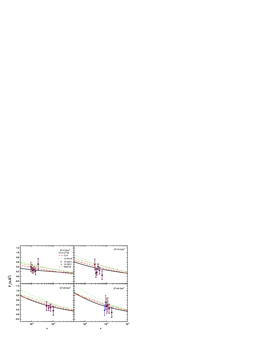
Figure 1: The longitudinal structure function $F_{L}(x,Q^{2})$ extracted from the parameterization of parton distributions at fixed $Q^{2}$ as a function of $x$ variable. The solid and dashed-dot-dot lines represent the CT18 [63] and the Mellin transforms method [15] at the NLO approximation respectively. The dashed and dot lines represent our predictions at $n_{f}=4$ and $n_{f}=3+c+b$ at the NLO approximation respectively. Experimental data (up-triangle H1 2014, down-triangle H1 2011 ) are from the H1-Collaboration [1,2] as accompanied with total errors.

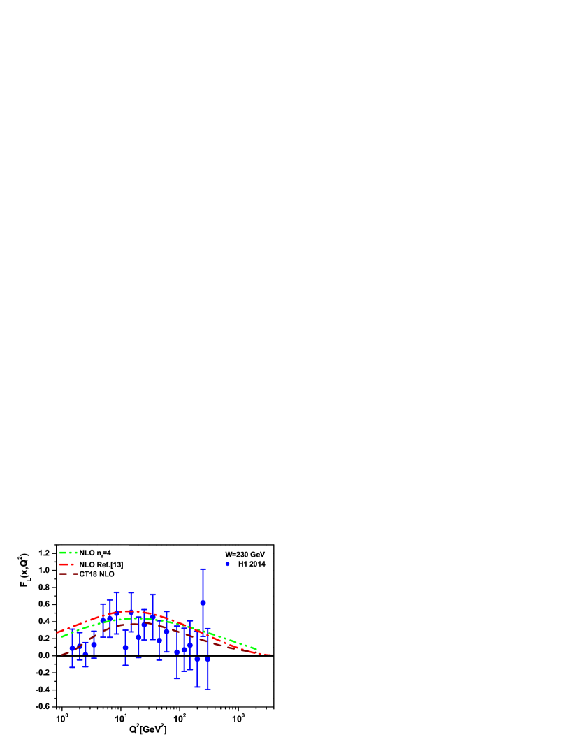
Figure 2: The obtained longitudinal structure function $F_{L}(x,Q^{2})$ from the parameterization of parton distributions as a function of variable $Q^{2}$ at fixed value of the invariant mass $W=230~{}\mathrm{GeV}$. The dashed and dashed-dot lines represent the CT18 [63] and the Mellin transforms method [15] at the NLO approximation. The dashed-dot-dot line represents our predictions at $n_{f}=4$ within the NLO approximation. Experimental data are from the H1-Collaboration [1] as accompanied with total errors.

Coefficients and more discussions about them can be seen in Refs.[11] and [12]. The massless distributions for $n_{f}=4$ and $n_{f}=5$ massless quarks are just $3/5$ and $6/11$ of $G_{nf=3}(x,Q^{2})$ [12]. In Ref.[15] the QCD parameter $\Lambda$ has been extracted due to $\alpha_{s}(M_{z}^{2})=0.1166$, which corresponds to the number of active flavor at NLO approximation as $\Lambda(n_{f}=5)=195.7~{}\mathrm{MeV},\Lambda(n_{f}=4)=284.0~{}\mathrm{MeV}$ and $\Lambda(n_{f}=3)=347.2~{}\mathrm{MeV}$.
With the explicit form of the distribution functions, I can proceed to extract the longitudinal structure function $F_{L}(x,Q^{2})$ from data mediated by the parametrization of $F_{2}(x,Q^{2})$ and $G_{n_{f}}(x,Q^{2})$. I have calculated the $x$-dependence of the longitudinal structure function at several fixed values of $Q^{2}$ corresponding to H1-Collaboration data [1,2]. Results are presented and compared with H1 data [1,2] and the parameterization of $F_{L}(x,Q^{2})$ [15] at NLO approximation in Fig.1. It is seen that, for all values of the presented $Q^{2}$, the extracted longitudinal structure function within the NLO approximation at $n_{f}=4$ is in a much better agreement with data and is comparable with the Mellin transforms method [13,14,15]. Also the impact of the gluon distribution due to the number of active flavor in the heavy-quark longitudinal structure function is considered. The running charm and bottom-quak masses are considered as $m_{c}=1.29~{}\mathrm{GeV}$ and $m_{b}=4.049~{}\mathrm{GeV}$ [62]. In order to present more detailed discussions on our findings, the results for the longitudinal structure function compared with CT18 [63] in this figure. As can be seen from the related figures, the longitudinal structure function results are consistent with the CT18 NLO at moderate and large values of $Q^{2}$.
In Fig.2, I have calculated the $Q^{2}$-dependence of the longitudinal structure function at low $x$ in the NLO approximation. Results of calculations and comparison with data of the H1-Collaboration [1,2] are presented in this figure (i.e., Fig.2), where the dashed-dot (Ref.[15]) and dashed-dot-dot (this work) lines correspond to the extracted $F_{L}(x,Q^{2})$ at $n_{f}=4$ in the NLO approximation, respectively. These results have been performed at fixed value of the invariant mass $W$ as $W=230~{}\mathrm{GeV}$. These results are compared with the CT18 NLO. Figure 2 shows that the parameterization of parton distributions provides correct behaviors of the extracted $F_{L}(x,Q^{2})$ within the NLO approximation. Over a wide range of variable $Q^{2}$, the extracted longitudinal structure functions are in a good agreement with experimental data in comparison with the parameterization of $F_{L}(x,Q^{2})$. At low values of $Q^{2}$, the extracted results are still above the experimental data. Although this result is consistent with the Mellin transforms method in this region.
In order to make sure these results are in the deep inelastic region, I use the nonlinear longitudinal structure function where effects of the nonlinear corrections to the gluon distribution are taken into account. The most important correction to the gluon distribution is the gluon recombination effect. For small momentum transfer the produced gluon overlap themselves in the transverse area and fusion processes, $gg{\rightarrow}g$, become important [64-70]. This gluon recombination effect is one of the important correction to the DGLAP equations [71,72,73] which theoretical predictions of this effect is initialled by Gribov, Levin and Ryskin [74] and followed by Mueller and Qiu (MQ) [75].
The GLR-MQ equation can be written in standard form [76,77,78]

$$\frac{\partial{G(x,Q^{2})}}{\partial{\ln}Q^{2}} = \frac{\partial{G(x,Q^{2})}}{\partial{\ln}Q^{2}}|_{DGLAP}$$ (13)

$$-\frac{81}{16}\frac{\alpha^{2}_{s}(Q^{2})}{\mathcal{R}^{2}Q^{2}}\int_{\chi}^{1}\frac{dz}{z}G^{2}(\frac{x}{z},Q^{2}),$$

where $\chi=\frac{x}{x_{0}}$ and $x_{0}$ is the boundary condition that the gluon distribution joints smoothly onto the linear region. The correlation length $\mathcal{R}$ determines the size of the nonlinear terms. This value depends on how the gluon ladders are coupled to the nucleon or on how the gluons are distributed within the nucleon. By solving GLR-MQ (i.e., Eq.13), the nonlinear correction to the gluon distribution function (i.e., $G_{n_{f}}^{\mathrm{NL}}(x,Q^{2})$ ) is obtained by the following form as

$$G_{n_{f}}^{\mathrm{NL}}(x,Q^{2}) = G_{n_{f}}^{\mathrm{NL}}(x,Q_{0}^{2})+G_{n_{f}}(x,Q^{2})-G_{n_{f}}(x,Q_{0}^{2})$$

$$-\int_{Q_{0}^{2}}^{Q^{2}}\frac{81}{16}\frac{\alpha^{2}_{s}(Q^{2})}{\mathcal{R}^{2}Q^{2}}\int_{\chi}^{1}\frac{dz}{z}G_{n_{f}}^{2}(\frac{x}{z},Q^{2})d{\ln}Q^{2}$$

At $Q_{0}^{2}$ the low $x$ behavior of the nonlinear gluon distribution is assumed to be [79,80,81]

$$G_{n_{f}}^{\mathrm{NL}}(x,Q_{0}^{2}) = G_{n_{f}}(x,Q_{0}^{2})\{1+\frac{27\pi{\alpha_{s}(Q_{0}^{2})}}{16\mathcal{R}^{2}Q_{0}^{2}}\theta(x_{0}-x)$$ (15)

$${\times}[G_{n_{f}}(x,Q_{0}^{2})-G_{n_{f}}(x_{0},Q_{0}^{2})]\}^{-1}.$$

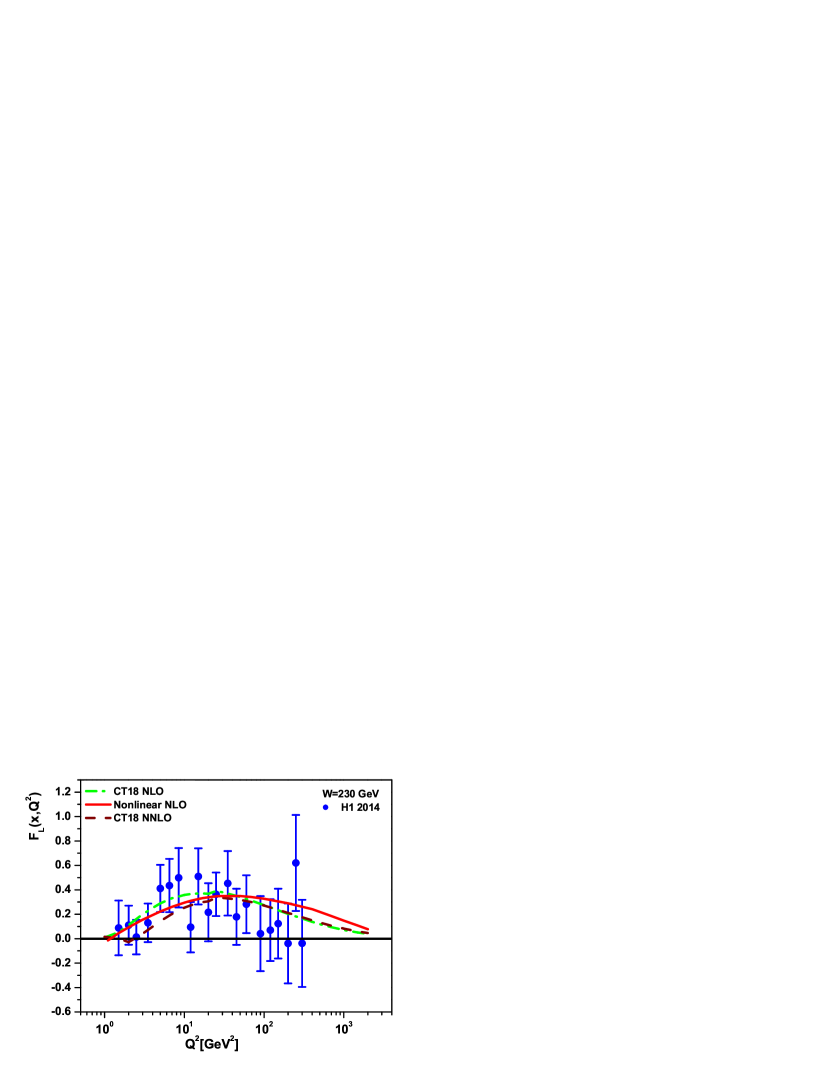
Figure 3: The obtained longitudinal structure function $F_{L}(x,Q^{2})$ from the nonlinear gluon distribution as a function of variable $Q^{2}$ at fixed value of the invariant mass $W=230~{}\mathrm{GeV}$ at hotspot point. The dashed and dashed-dot lines represent the CT18 [63] at the NNLO and NLO approximation respectively. The solid line represents nonlinear behavior of the longitudinal structure function at $n_{f}=4$ within the NLO approximation. Experimental data are from the H1-Collaboration [1] as accompanied with total errors.

In Fig.3, AM equation with GLR-MQ correction is used to evaluate the longitudinal structure function at low $x$ and $Q^{2}$. As can be seen in Fig.3, the nonlinear correction is very important to slow down the longitudinal structure function behavior at low $Q^{2}$ values. The evolutions of the nonlinear correction to $F_{L}$ with $Q^{2}$ at fixed value of the invariant mass $W$ and the comparisons with the experimental data [1] and CT18 [63] are shown in Fig.3. A comparison between Figs.2 and 3 shows that the nonlinear effects of the longitudinal structure function are observable for $x<x_{0}=0.01$ at hotspot point where gluons are populated across the proton as it is equal to $\mathcal{R}\simeq 2~{}\mathrm{GeV}^{-1}$. As can be seen, the nonlinear results at hot spot point at low and moderate $Q^{2}$ values seem to be compatible with the H1 data and CT18 at NLO and NNLO approximations. Indeed he nonlinear corrections here are negative and result in a better agreement with data and parameterization method.
To summarize, I used the parton parameterization method suggested in Refs.[11,12] to obtain the longitudinal structure function. The method depends on the number of active flavor as the results are considered in two cases $n_{f}=4$ and $n_{f}=3+c+b$. The heavy flavor contributions to the longitudinal structure function are taken as $Q^{2}$ increases above about $m^{2}_{c}$ and then above about $m^{2}_{b}$. Dependent gluon distributions are usually are given in a parameterization method in which the number of active quark flavors increases from $n_{f}=3$ to $n_{f}=4$ and then to $n_{f}=5$ corresponds to the threshold heavy quark production, which are directly related to the gluon density in the photo-gluon fusion reactions. I have applied the nonlinear correction to extract the longitudinal structure function at low values of $x$. It has been found that at low and moderated $Q^{2}$, NLO results are corresponding to the experimental data and other parameterization methods.

.1 ACKNOWLEDGMENTS

The author is thankful to Razi University for financial support of this project. The author is especially grateful to A.V.Kotikov for carefully reading the manuscript and for critical notes. Thanks also go to H.Khanpour for help with preparation of the QCD parametrization model.

Table 1: Parameters of Eq.(8) [12], resulting from a global fit to the ZEUS data.

parameters                    value
$a_{0}$	$-7.828\times 10^{-2}\pm 5.19\times 10^{-3}$
$a_{1}$	$2.248\times 10^{-2}\quad\pm 1.47\times 10^{-3}$
$a_{2}$	$2.301\times 10^{-4}\pm 4.88\times 10^{-4}$
$b_{0}$	$1.313\times 10^{-2}\pm 6.99\times 10^{-4}$
$b_{1}$	$4.736\times 10^{-3}\pm 2.98\times 10^{-4}$
$b_{2}$	$1.064\times 10^{-3}\pm 3.88\times 10^{-5}$
$F_{p}$	$0.503\pm 0.0012$
$x_{p}$	$0.0494\pm 0.0039$
$\chi^{2}(\mathrm{goodness~{}of~{}fit})$	$1.11$

.2 References

1. H1 Collab. (V.Andreev , A.Baghdasaryan, S.Baghdasaryan et al.), Eur.Phys.J.C74, 2814(2014).
2. H1 Collab. (F.D.Aaron , C.Alexa, V.Andreev et al.),Eur.Phys.J.C71, 1579 (2011).
3. ZEUS Collab. (H.Abramowicz , I.Abt, L.Adamczyk et al.), Phys.Rev.D90, 072002 (2014).
4. P.Agostini , H.Aksakal, H.Alan et al. [LHeC Collaboration and FCC-he Study Group ], CERN-ACC-Note-2020-0002, arXiv:2007.14491 [hep-ex] (2020).
5. J.Bartels, K.Golec-Biernat and L.Motyka, Phys.Rev. D81, 054017 (2010).
6. V.Tvaskis , A.Tvaskis, I.Niculescu et al., Phys.Rev.C97, 045204(2018).
7. V.Chekelian, arXiv [hep-ex]:0810.5112 (2008).
8. G.Altarelli and G. Martinelli, Phys.Lett.B76, 89(1978).
9. R.S.Thorne, arXiv:hep-ph/9805298(1998).
10. A.D.Martin W.J.Stirling and R.S.Thorne, Phys.Lett.B636, 259(2006).
11. M.M.Block, L.Durand and D.W.McKay, Phys.Rev.D77, 094003(2008).
12. M.M.Block and L.Durand, arXiv: 0902.0372 [hep-ph](2009).
13. L.P.Kaptari , A.V.Kotikov, N.Yu.Chernikova and P.Zhang, JETP Lett.109, 281(2019).
14. A.V.Kotikov, JETP Lett.111, 67 (2020).
15. L.P.Kaptari , A.V.Kotikov, N.Yu.Chernikova and P.Zhang, Phys.Rev.D99, 096019(2019).
16. B. Rezaei and G.R. Boroun, Eur.Phys.J.A56, 262 (2020).
17. G.R. Boroun, Phys.Rev.C97, 015206 (2018).
18. G.R. Boroun, Eur.Phys.J.Plus129, 19 (2014).
19. G.R. Boroun and B. Rezaei, Eur.Phys.J.C72, 2221 (2012).
20. N. Baruah, M.K. Das and J.K. Sarma, Eur.Phys.J.Plus129, 229 (2014).
21. G.R.Boroun and B.Rezaei, EPL,133, 61002 (2021).
22. G.R.Boroun, Chin.Phys.C45, 063105 (2021).
23. G.R.Boroun and B.Rezaei, Phys.Lett.B816, 136274 (2021).
24. G.R.Boroun, Eur.Phys.J.Plus135, 68(2020).
25. G.R.Boroun and B.Rezaei, Nucl.Phys.A1006, 122062(2021).
26. B.Rezaei and G.R.Boroun, Commun.Theor.Phys.59, 462 (2013).
27. G.R.Boroun and B.Rezaei, Eur.Phys.J.C72, 2221 (2012).
28. B.Rezaei and G.R.Boroun, Nucl.Phys.A857, 42(2011).
29. G.R.Boroun, Int.J.Mod.Phys.E18, 131(2009).
30. S.Moch, J.A.M.Vermaseren and A.Vogt, Phys.Lett.B606, 123(2005).
31. S.Alekhin, J.Bl$\ddot{\mathrm{u}}$mlein and S.-O.Moch, arXiv[hep-ph]:1808.08404 (2018).
32. A.M.Cooper-Sarkar, R.C.E.Devenish and A.De Roeck, Int.J.Mod.Phys.A13, 3385 (1998).
33. R.Thorne, Phys.Rev.D73, 054019 (2006).
34. R.Thorne, Phys.Rev.D86, 074017 (2012).
35. S.Alekhin, J. Bl$\ddot{\mathrm{u}}$mlein, S. Klein and S. Moch , arXiv [hep-ph]:0908.3128(2009).
36. G.Beuf, C.Royon and D.Salek, arXiv[hep-ph]:0810.5082(2008).
37. J.Bl$\ddot{\mathrm{u}}$mlein, A.De Freitas, C.Schneider and K.Sch$\ddot{\mathrm{o}}$nwald, Phys. Lett.B782, 362(2018).
38. S.Alekhin, J. Bl$\ddot{\mathrm{u}}$mlein and S. Moch, arXiv [hep-ph]:2006.07032(2020).
39. M.Gl$\mathrm{\ddot{u}}$ck, C.Pisano and E.Reya, Phys.Rev.D77, 074002(2008).
40. S.Riemersma, J.Smith and W.L.van Neerven, Phys.Lett.B347, 143(1995).
41. A.V.Kisselev, Phys.Rev.D60, 074001(1999).
42. E.Laenen, S.Riemersma, J.Smith and W.L. van Neerven, Nucl.Phys.B392, 162(1993).
43. A.Y.Illarionov, B.A.Kniehl and A.V.Kotikov, Phys.Lett.B663, 66 (2008).
44. S.Catani and F.Hautmann, Nucl. Phys.B427, 475(1994).
45. Wu-Ki Tung, S. Kretzer, and C. Schmidt, J. Phys. G 28, 983 (2002).
46. G.R. Boroun, B. Rezaei and J.K. Sarma, Int.J.Mod.Phys.A29 (2014) 32, 1450189.
47. G.R. Boroun and B. Rezaei, Nucl.Phys.A929, 119(2014).
48. G.R. Boroun, Nucl.Phys.B884, 684(2014).
49. G.R.Boroun, PoSHQL2012(2012)069.
50. G.R. Boroun and B. Rezaei, EPL100, 41001(2012).
51. G.R. Boroun and B. Rezaei, Nucl.Phys.B857, 143(2012).
52. G.R. Boroun and B. Rezaei, J.Exp.Theor.Phys.115, 427(2012).
53. Ali N. Khorramian, S. Atashbar Tehrani and A. Mirjalili, Nucl.Phys.B Proc.Suppl.186, 379 (2009).
54. S.Khatibi and H.Khanpour, Nucl.Phys.B967, 115432 (2021).
55. J.Blumlein, A.De Freitas, W.L. van Neerven and S.Klein, Nucl.Phys.B755, 272 (2006).
56. H.Khanpour, Nucl.Phys.B958, 115141 (2020).
57. H.Khanpour,Phys.Rev.D99, 054007 (2019).
58. G.R.Boroun, Phys.Lett.B744, 142 (2015).
59. G.R.Boroun, Phys.Lett.B741, 197 (2015).
60. A.V.Kotikov, A.V.Lipatov and P.Zhang, arXiv [hep-ph]:2104.13462 (2021).
61. H1 and ZEUS Collab. (F.D.Aaron, H.Abramowicz, I.Abt et al.), JHEP 1001, 109 (2010).
62. H1 and ZEUS Collab. (H.Abramowicz, I.Abt, L.Adamczyk et al.), Eur.Phys.J.C78, 473(2018).
63. Tie-Jiun Hou et al., Phys.Rev.D103, 014013(2021).
64. A.V.Giannini and F.O.Dur$\widetilde{a}$es, Phys.Rev.D88, 114004(2013).
65. G.R.Boroun and B.Rezaei, arXiv [hep-ph]:2105.01121 (2021).
66. R.Wang and X.Chen, Chinese Phys.C41, 053103(2017).
67. G.R.Boroun and S.Zarrin, Eur.Phys.J.Plus128, 119(2013).
68. B.Rezaei and G.R.Boroun, Phys.Lett.B692, 247(2010).
69. G.R.Boroun, Eur.Phys.J.A43, 335(2010).
70. G.R.Boroun, Eur.Phys.J.A42, 251(2009).
71. Y. L. Dokshitzer, Sov. Phys. JETP46, 641 (1977).
72. V. N. Gribov and L. N. Lipatov, Sov. J. Nucl. Phys.15, 438 (1972).
73. G. Altarelli and G. Parisi, Nucl. Phys. B 126, 298 (1977).
74. L. V. Gribov, E. M. Levin and M. G. Ryskin, Phys. Rep. 100, 1 (1983).
75. A. H. Mueller and Jianwei Qiu, Nucl. Phys. B 268, 427 (1986).
76. K.Prytz, Eur.Phys.J.C22, 317(2001).
77. K.J.Eskola,H.Honkanen, V.J.Kolhinen, J.Qiu and C.A.Salgado, Nucl.Phys.B660, 211(2003).
78. M.A Kimber, J.Kwiecinski and A.D.Martin, Phys.Lett.B508, 58(2001).
79. A.D.Martin, W.J Stirling and R.G Roberts, Phys.Rev.D47, 867(1993).
80. J.Kwiecinski, A.D.Martin and P.J.Sutton, Phys.Rev.D44, 2640(1991).
81. A.J.Askew, J.Kwiecinski, A.D.Martin and P.J.Sutton, Phys.Rev.D47, 3775(1993).