Topological Toda lattice and nonlinear bulk-edge correspondence

Abstract

The Toda lattice is a model of nonlinear wave equations allowing exact soliton solutions. It is realized by an electric circuit made of a transmission line with variable capacitance diodes and inductors. It has been generalized to the dimerized Toda lattice by introducing alternating bondings specified by a certain parameter $\lambda$, where it is reduced to the Toda lattice at $\lambda=0$. In this work, we investigate the topological dynamics of the voltage along the transmission line. It is demonstrated numerically that the system is topological for $\lambda<0$, while it is trivial for $\lambda>0$ with the phase transition point given by the original Toda lattice ($\lambda=0$). These topological behaviors are well explained by the chiral index familiar in the Su-Schrieffer-Heeger model. The topological phase transition is observable by a significant difference between the dynamics of voltages in the two phases, which is explained by the emergence of the topological edge states. This is a bulk-edge correspondence in nonlinear systems. The dimerized Toda lattice is adiabatically connected to a linear system, which would be the reason why the topological arguments are valid. Furthermore, we show that the topological edge state is robust against randomness.

Introduction: Topological insulators is one of the most intensively studied topics in condensed matter physicsHasan ; Qi . The emergence of topological edge states is characteristic to a topological phase, as is the bulk-edge correspondence. They are conveniently realized in electric circuitsTECNature ; ComPhys ; Hel ; Lu ; YLi ; EzawaTEC ; Research ; Zhao ; EzawaLCR ; EzawaSkin ; Garcia ; Hofmann ; EzawaMajo ; Tjunc ; Lee . It is based on the fact that we can construct such a circuit Laplacian that is equivalent to the Hamiltonian. Thus, a circuit Laplacian may have topological phases. Here, topological edge states are observed by impedance peaks. There is also an application to dynamical systems. A quantum walk may be described by the time evolution of the voltage in an electric circuit, because the Kirchhoff law is rewritten in the form of the Scrödinger equationQWalk ; EzawaUniv ; EzawaDirac . Here, the emergence of a topological edge state is observable by a peculiar behavior of a quantum walker, i.e., by a peculiar time evolution of the voltage. The topological physics has so far been mainly studied in linear systems. One of the merit of electric circuits is that we can naturally introduce nonlinear elements into circuits. It is an interesting problem to study topological properties in nonlinear systemsKot ; Sone .

The Toda lattice is one of the most famous exactly solvable nonlinear modelsToda ; Toda2 ; Toda3 . The Toda lattice with alternating bonding is called the dimerized Toda latticeKofane ; Pelap , where soliton solutions seem to be absentLus . This is not surprising because the Toda soliton is nontopological and fragile against perturbations. It is known that the Toda lattice is realized by a transmission line consisting of variable capacitance diodes and inductorsHirota ; Singer ; Yemele ; Yemele2 ; Pelap05 ; Houwe . When the inductance is alternating, it is generalized to the dimerized Toda latticeKofane ; Pelap . So far there is no study on topological properties of the Toda lattice.

In this paper, we explore the topological aspect of the dynamics governed by the nonlinear wave equation associated with the dimerized Toda lattice. Interestingly we find that the nonlinear wave equation contains a term proportional to the Su-Schrieffer-Heeger (SSH) Hamiltonian. We wonder if the dynamics is characterized by the topological number inherent to the SSH model. The main issue of this work is to study this problem. We solve the time evolution of the voltage along the transmission line numerically in nonlinear models, by applying a voltage only at its edge as an initial condition. We demonstrate that the dynamical behaviors are quite distinct in the topological and trivial phases assigned by a topological number defined in the SSH Hamiltonian. The voltage shows a standing wave at the edge in the topological phase but it rapidly decreases in the trivial phase. These distinct behaviors are interpreted by the emergence of the topological edge states, namely, by the bulk-edge correspondence in nonlinear systems. This would be due to the fact that the nonlinear system is adiabatically connected to the linear-wave system described by the SSH model. The topological phase transition point corresponds to the original Toda lattice, which is unchanged by the strength of nonlinearity. Finally, we check numerically that the topological edge states are robust against randomness in inductance.

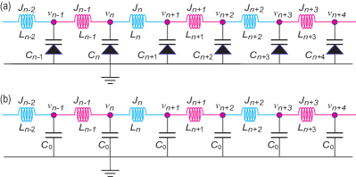
Figure 1: Illustration of a transmission line made of (a) nonlinear elements realizing the site-dependent Toda lattice and (b) linear elements realizing the telegrapher equation. The inductance is alternating, as indicated by magenta and cyan colors. Each node is grounded via a variable capacitance diode and a capacitor in (a) and (b), respectively.

Dimerized Toda Lattice: The Toda equationToda ; Toda2 is well realized by a transmission line with variable capacitance diodes and inductorsHirota as shown in Fig.1(a). The Kirchhoff law is described by

$$L_{n}\frac{dJ_{n}}{dt}=v_{n}-v_{n+1},\quad\quad\frac{dQ_{n}}{dt}=J_{n-1}-J_{n},$$ (1)

where $v_{n}$ is the voltage, $J_{n}$ is the current and $Q_{n}$ is the charge at the node $n$, while $L_{n}$ is the inductance for the inductor between the nodes $n$ and $n+1$, as illustrated in Fig.1(a). The Kirchhoff law is summarized in the form of the second-order differential equation,

$$\frac{d^{2}Q_{n}}{dt^{2}}=\frac{1}{L_{n-1}}\left(V_{n-1}-V_{n}\right)-\frac{1}{L_{n}}\left(V_{n}-V_{n+1}\right),$$ (2)

where we have introduced a new variable $V_{n}$ by $v_{n}=V_{0}+V_{n}$. The capacitance is a function of the voltage $V_{n}$ in the variable capacitance diode, and it is well given by $C\left(V_{n}\right)=Q\left(V_{0}\right)/\left(F_{0}+V_{n}-V_{0}\right)$, where $F_{0}$ is a constant characteristic to the variable capacitance diodeNakajima .

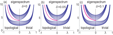
Figure 2: (a)$\sim$(c) Eigenspectrum of $M_{nm}$ as a function of $\lambda$. The edge states emerge for $\lambda<0$, as shown by magenta curves. (a) Pure system ($\delta=0$). (b) and (c) System with randomness $(\delta\not=0)$.

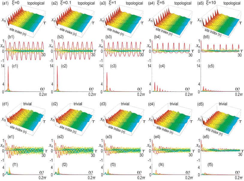
Figure 3: Time evolution of the dimensionless voltage $x_{n}$ in the nonlinear telegrapher equation. The horizontal axis is the dimensionless time $\tau$ ranging $0\leq\tau\leq 30$. (a1)$\sim$(c5) Topological phase ($\lambda=-0.5$). (d1)$\sim$(f5) Trivial phase ($\lambda=0.5$). (a1)$\sim$(a5) and (d1)$\sim$(d5) Bird’s eye’s view of the time evolution. (b1)$\sim$(b5) and (e1)$\sim$(e5) Color plot of the time evolution. (c1)$\sim$(c5) and (f1)$\sim$(f5) Fourier components in the frequency $\omega$. The red (cyan) curve represents the voltage at the left (right) edge. We have set $\xi=0$ for (a1)$\sim$(f1), $\xi=0$ for (a2)$\sim$(f2), $\xi=1$ for (a3)$\sim$(f3) , $\xi=5$ for (a4)$\sim$(f4) and $\xi=10$ for (a5)$\sim$(f5).

The charge is given by

$$Q_{n}=\int_{0}^{V_{n}}C\left(V\right)dV=Q\left(V_{0}\right)\log\left[1+V_{n}F_{0}^{-1}\right]+\text{const.}$$ (3)

A closed form of the differential equation for $V_{n}$ follows from Eqs.(2) and (3),

$$Q\left(V_{0}\right)\frac{d^{2}}{dt^{2}} \log\left[1+V_{n}F_{0}^{-1}\right]$$

$$=\frac{V_{n+1}}{L_{n}}-\left(\frac{1}{L_{n-1}}+\frac{1}{L_{n}}\right)V_{n}+\frac{V_{n-1}}{L_{n-1}}.$$ (4)

When we set $L_{n}=L$ for all $n$, it is reduced to

$$Q\left(V_{0}\right)\frac{d^{2}}{dt^{2}}\log\left[1+V_{n}F_{0}^{-1}\right]=\frac{1}{L}\left(V_{n+1}-2V_{n}+V_{n-1}\right).$$ (5)

This is the Toda equation.

We focus on the dimerized Toda lattice defined by setting $L_{2n-1}=L-\ell$, $L_{2n}=L+\ell$, as corresponds to the inductance alternating, where $\left|\ell\right|<L$. We rewrite Eq.(4) as

$$\frac{1}{\xi}\frac{d^{2}}{d\tau^{2}} \log\left[1+\xi x_{2n-1}\right]$$

$$=t_{A}x_{2n}-\left(t_{A}+t_{B}\right)x_{2n-1}+t_{B}x_{2n-2},$$ (6)

$$\frac{1}{\xi}\frac{d^{2}}{d\tau^{2}} \log\left[1+\xi x_{2n}\right]$$

$$=t_{B}x_{2n+1}-\left(t_{A}+t_{B}\right)x_{2n}+t_{A}x_{2n-1},$$ (7)

where we have introduced dimensionless quantities,

$$\tau = t/\sqrt{LQ\left(V_{0}\right)V_{1}^{2}/F_{0}},\quad x_{n}=V_{n}/V_{1},$$

$$\xi = V_{1}/F_{0},\quad\lambda=\ell/L.$$ (8)

They are dimensionless time, voltage, nonlinearity parameter and dimerization parameter, respectively. We have defined $t_{A}=1/(1-\lambda)$ and $t_{B}=1/\left(1+\lambda\right)$, where $A$ and $B$ denote the sublattice indices. Eqs.(6) and (7) are summarize as

$$\frac{1}{\xi}\frac{d^{2}}{dt^{2}}\left(\log\left[1+\xi x_{n}\right]\right)=M_{nm}x_{m},$$ (9)

with a tridiagonal matrix $M_{nm}$, where the nonlinearity is controlled by $\xi$.

We make a Fourier transformation from the node index $n$ to the momentum $k$ by setting $x_{A}\left(k\right)=N^{-1/2}\sum_{n=1}x_{2n-1}e^{ink}$ and $x_{B}\left(k\right)=N^{-1/2}\sum_{n=1}x_{2n}e^{ink}$, to find that

$$\frac{1}{\xi}\frac{d^{2}}{d\tau^{2}} \left(\begin{array}[]{c}\log\left[1+\xi\sum_{k}x_{A}\left(k\right)e^{-ink}\right]\\ \log\left[1+\xi\sum_{k}x_{B}\left(k\right)e^{-ink}\right]\end{array}\right)$$ (12)

$$\qquad\qquad=\sum_{k}M\left(k\right)\left(\begin{array}[]{c}x_{A}\left(k\right)\\ x_{B}\left(k\right)\end{array}\right)e^{-ink},$$ (15)

with

$$M\left(k\right)=-\left(t_{A}+t_{B}\right)I_{2}+\left(\begin{array}[]{cc}0&t_{A}+t_{B}e^{-ik}\\ t_{A}+t_{B}e^{-ik}&0\end{array}\right).$$ (16)

Here, $M\left(k\right)$ is identical to the SSH Hamiltonian up to a constant term.

The dimerized Toda equation (9) is reduced to a dimerized linear wave equation for $\xi\rightarrow 0$,

$$\frac{d^{2}}{d\tau^{2}}\left(\begin{array}[]{c}x_{A}\left(k\right)\\ x_{B}\left(k\right)\end{array}\right)=M\left(k\right)\left(\begin{array}[]{c}x_{A}\left(k\right)\\ x_{B}\left(k\right)\end{array}\right).$$ (17)

Correspondingly, a nonlinear transmission line [Fig.1(a)] is reduced to a linear transmission line [Fig.1(b)]. The topological properties of this linear wave equation have been studied in a transmission lineQWalk and also in acoustic systemsProdan ; Lubensky ; Nash ; Sus ; Kariyado ; Takahashi ; Mee ; Abba ; Mat .

Topological number: The topological number for the SSH model is defined by the chiral index,

$$\Gamma=\int_{0}^{2\pi}\text{Tr}\left[\sigma_{z}M^{-1}\left(k\right)\partial_{k}M\left(k\right)\right]dk.$$ (18)

Indeed, it is quantized, i.e., $\Gamma=1$ for $\left|t_{a}\right|<\left|t_{b}\right|$ and $\Gamma=0$ for $\left|t_{a}\right|>\left|t_{b}\right|$. Namely, the system is topological for $\lambda<0$ and trivial for $\lambda>0$. We show the eigenvalue of $M(k)$ for a finite chain in Fig.2(a), where the emergence of topological edge states is manifest for $\lambda<0$, as marked in red. Characteristic topological properties are induced by topological edge states.

Dynamics: The main issue of the present work is to inquire whether the nonlinear system (9) is also characterized by the topological number (18). First of all, let us make the following speculation. The left-hand side of Eq.(9) is a monotonic smooth function for $\xi$. It indicates that there is no phase transition in the parameter $\xi$. Hence, we expect that the topological properties will be inherited to the nonlinear system ($\xi\neq 0$) from the linear system ($\xi=0$).

In order to justify this speculation, we solve the nonlinear wave equation (9) as well as the linear one ($\xi=0$) numerically under the initial condition that we apply a nonzero voltage only at the left edge. We present numerical results for the nonlinearity $\xi=0$, $0.1$, $1$, $5$ and $10$ in two typical phases at $\lambda=\mp 0.5$ in Fig.3. In a topological phase ($\lambda=-0.5$), we observe a clear standing wave displayed in red, which is due to the topological edge state. Although the amplitude decreases as the nonlinearity $\xi$ increases, the overall structure remains unchanged. On the other hand, there is no standing wave in a trivial phase ($\lambda=0.5$), irrespective of the nonlinearity.

These properties are made clearer by making the Fourier analysis in frequency $\omega$. We focus on the topological phase: See Fig.3(c1)$\sim$(c5). In the linear regime ($\xi=0$), there is a single strong peak, which remains as it is in weak nonlinear regime ($\xi=0.1$). In strong nonlinear regime ($\xi\geq 5$), many satelite peaks emerge at the harmonic overtone frequencies. The intensity of the primal peak decreases in strong nonlinear regime due to the emergence of the satellite peaks. Such an effect of the nonlinearity manifests itself in the Fourier decomposition. On the other hand, all peaks are quite tiny irrespective of the linear or nonlinear regime and furthermore we do not see overtone satellite peaks in the trivial phase, as in Fig.3(f1)$\sim$(f5).

These behaviors are actually independent of $\lambda$, although the amplitude may change. To show it, we show the amplitude at the left edge as a function of $\lambda$ in Fig.4, where the topological phase transition is clearly observed at $\lambda=0$ independent of nonlinearity $\xi$.

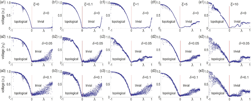
Figure 4: Amplitude of the dimensionless voltage $x_{1}$ at the left edge after long enough time. The horizontal axis is $\lambda$: The system is topological (trivial) for $\lambda<0$ ($\lambda>0$). (a1)$\sim$(a3) $\xi=0$, (b1)$\sim$(b3) $\xi=0.1$, (c1)$\sim$(c3) $\xi=1$, (d1)$\sim$(d3) $\xi=5$, and (e1)$\sim$(e3) $\xi=10$. (a1)$\sim$(a3) Pure system ($\delta=0$); (a2)$\sim$(e2) 5% randomness ($\delta=0.05$); (a3)$\sim$ (e3) 10% randomness in inductance ($\delta=0.1$).

Bulk-edge correspondence: These results are interpreted as follows.Once we start with a voltage localized initially at one edge, there remains a finite voltage at the edge in the topological phase. This is because the topological edge mode is almost isolated from all other modes, although a certain amount of voltage propagates into the chain. The amount of voltage lost from the edge becomes larger as the nonlinearity $\xi$ increases. On the other hand, since there is no localized edge mode in the trivial phase, almost all amounts of voltage applied at the edge propagate into the chain. These results are manifestation of the nonlinear bulk-edge correspondence in physical observable quantities.

Randomness effect: We study how the topological dynamics is robust against randomness in inductors. We have introduced randomness into inductors uniformly distributing from $-\delta$ to $\delta$ by the procedure $L\pm\ell\longmapsto\left(L\pm\ell\right)\left(1+\eta\delta\right)$, where $\eta$ is a random variable ranging from $-1$ to $1$. Numerical results are shown in Figs.2, 3 and 4 for some values of $\delta$. Clearly the dynamics is almost identical between the pure system and disordered systems, which indicates that the topological edge states are robust against randomness. On the other hand, there is a new phenomenon due to randomness in the trivial phase, where the amplitude becomes nonvanishing. This is because the voltage propagation is localized due to the randomness, which is a reminiscence of the Anderson localizationAnder .

Comments are in order. (i) The amplitude becomes large around $\lambda\simeq 1$ in Fig.4, although the system is trivial. In this parameter region, the system is almost dimerized, where the voltage cannot propagate into the bulk. (ii) The amplitude takes the minimum at $\lambda=0$ irrespective of the nonlinearity $\xi$ and the disorder $\delta$ in Fig.4. This phenomenon would be due to the existence of a Toda soliton at $\lambda=0$ for all $\xi$. The soliton moves with a constant velocity, which means that the voltage at the edge rapidly decreases as a function of time. Furthermore, the soliton dynamics is robust for disorders. Hence, the topological phase transition is rigid for all $\xi$ and $\delta$.

Discussion: The topological analysis is familiar in condensed matter physics and also in linear systems such as electric circuits and acoustic systems. However, it is highly nontrivial in nonlinear systems, where a general argument would be formidable. It would be necessary to make individual study in various typical models.

In this work we have made a first step toward the problem by taking the dimerized Toda lattice model, where we have identified a parameter controlling nonlinearity. An important feature is that the model has an adiabatic connectivity to a linear system governed by the SSH model. We have carried out a numerical analysis to show that the bulk-edge correspondence is inherited from the linear system to the nonlinear system. Indeed, we have numerically checked in Figs.3 and 4 that the topological dynamics in nonlinear systems is the same as the one in the linear system. We may conclude that the topological number well captures the topological dynamics in the dimerized Toda lattice. Our scheme will be applicable to make topological analysis in other nonlinear systems.

The author is very much grateful to M. Kawamura, S. Katsumoto, Pierre Delplace and N. Nagaosa for helpful discussions on the subject. This work is supported by the Grants-in-Aid for Scientific Research from MEXT KAKENHI (Grants No. JP17K05490 and No. JP18H03676). This work is also supported by CREST, JST (JPMJCR16F1 and JPMJCR20T2).

References

- (1) M. Z. Hasan and C. L. Kane, Rev. Mod. Phys. 82, 3045 (2010).
- (2) X.-L. Qi and S.-C. Zhang, Rev. Mod. Phys. 83, 1057 (2011).
- (3) S. Imhof, C. Berger, F. Bayer, J. Brehm, L. Molenkamp, T. Kiessling, F. Schindler, C. H. Lee, M. Greiter, T. Neupert, R. Thomale, Nat. Phys. 14, 925 (2018).
- (4) C. H. Lee , S. Imhof, C. Berger, F. Bayer, J. Brehm, L. W. Molenkamp, T. Kiessling and R. Thomale, Communications Physics, 1, 39 (2018).
- (5) T. Helbig, T. Hofmann, C. H. Lee, R. Thomale, S. Imhof, L. W. Molenkamp and T. Kiessling, Phys. Rev. B 99, 161114 (2019).
- (6) Y. Lu, N. Jia, L. Su, C. Owens, G. Juzeliunas, D. I. Schuster and J. Simon, Phys. Rev. B 99, 020302 (2019).
- (7) K. Luo, R. Yu and H. Weng, Research (2018), ID 6793752.
- (8) E. Zhao, Ann. Phys. 399, 289 (2018).
- (9) Y. Li, Y. Sun, W. Zhu, Z. Guo, J. Jiang, T. Kariyado, H. Chen and X. Hu, Nat. Com. 9, 4598 (2018)
- (10) M. Ezawa, Phys. Rev. B 98, 201402(R) (2018).
- (11) M. Serra-Garcia, R. Susstrunk and S. D. Huber, Phys. Rev. B 99, 020304 (2019).
- (12) T. Hofmann, T. Helbig, C. H. Lee, M. Greiter, R. Thomale, Phys. Rev. Lett. 122, 247702 (2019).
- (13) M. Ezawa, Phys. Rev. B 100, 045407 (2019).
- (14) M. Ezawa, Phys. Rev. B 99, 201411(R) (2019).
- (15) M. Ezawa, Phys. Rev. B 99, 121411(R) (2019).
- (16) M. Ezawa, Phys. Rev. B 102, 075424 (2020).
- (17) C. H. Lee, T. Hofmann, T. Helbig, Y. Liu, X. Zhang, M. Greiter and R. Thomale, Nature Communications 11, 4385 (2020).
- (18) M. Ezawa, Phys. Rev. B 100, 165419 (2019).
- (19) M. Ezawa, Phys. Rev. Research 2, 023278 (2020).
- (20) M. Ezawa, J. Phys. Soc. Jpn. 89, 124712 (2020).
- (21) T. Kotwal, H. Ronellenfitsch, F. Moseley, A. Stegmaier, R. Thomale, J. Dunkel, arXiv:1903.10130
- (22) K. Sone, Y. Ashida, T. Sagawa, arXiv:2012.09479
- (23) M. Toda, J. Phys. Soc. Jpn. 22, 431 (1967).
- (24) M. Toda, Springer Ser. Solid State Sci. 20, Springer, Berlin, (1981).
- (25) M. Toda, Proc. Jpn. Acad. Ser. B 80, 445 (2004).
- (26) T. Kofane, B. Michaux and M. Remoissenet, J. Phys. C: Solid State Phys. 21, 1395 (1988).
- (27) F. B. Pelap, T. C. Konafe, N. Flytzania and M. Remoissenet, J. Phys. Soc. Jpn. 70, 2568 (2001).
- (28) C. J. Lustri and M. A. Porter, SIAM J. Appl. Dynamical Systems c 17 1182 (2016)
- (29) R. Hirota and K. Suzuki, J. Phys. Soc. Jpn. 28, 1366 (1970).
- (30) H. Nagashima and Y. Amagishi, J. Phys. Soc. Jpn. 45, 680 (1978).
- (31) A. C. Singer and A. V. Oppenheim, Int. J. Bifurcation and Chaos 09, 571 (1999)
- (32) D. Yemele, P. Marquie and J. Marie Bilbault, Phys. Rev. E 68, 016605 (2003)
- (33) D. Yemele, P. K. Talla and T. C. Kofané, J. Phys. D: Appl. Phys. 36, 1429 (2003)
- (34) F. B. Pelap and M. M. Faye, J. Math. Phys. 46, 033502 (2005)
- (35) A. Houwe, S. Abbagari, M. Inc, G. Betchewe, S. Y. Doka, K. T. Crepin, K.S. Nisar, Results in Physics 18, 203188 (2020)
- (36) E. Prodan and C. Prodan, Phys. Rev. Lett. 103, 248101 (2009).
- (37) C. L. Kane and T. C. Lubensky, Nature Phys. 10, 39 (2014).
- (38) L. M. Nash, D. Kleckner, A. Read, V. Vitelli, A. M. Turner and W. T. M. Irvine, PNAS 112, 14495 (2015).
- (39) R. Susstrunk, S. D. Huber, Science 349, 47 (2015).
- (40) T. Kariyado and Y. Hatsugai, Sci. Rep. 5, 18107 (2016).
- (41) Y. Takahashi, T. Kariyado and Y. Hatsugai, New J. Phys. 19, 035003 (2017).
- (42) A. S. Meeussen, J. Paulose and V. Vitelli, Phys. Rev. X 6, 041029 (2016).
- (43) H. Abbaszadeh, A. Souslov, J. Paulose, H. Schomerus and V. Vitelli, Phys. Rev. Lett. 119, 195502 (2017).
- (44) K. H. Matlack, M. Serra-Garcia, A. Palermo, S. D. Huber and C. Daraio, Nature Mat. 17, 323 (2018).
- (45) M. Ezawa, arXiv:2106.07147