Spectral Pruning for Recurrent Neural Networks

Abstract

Recurrent neural networks (RNNs) are a class of neural networks used in sequential tasks. However, in general, RNNs have a large number of parameters and involve enormous computational costs by repeating the recurrent structures in many time steps. As a method to overcome this difficulty, RNN pruning has attracted increasing attention in recent years, and it brings us benefits in terms of the reduction of computational cost as the time step progresses. However, most existing methods of RNN pruning are heuristic. The purpose of this paper is to study the theoretical scheme for RNN pruning method. We propose an appropriate pruning algorithm for RNNs inspired by “spectral pruning”, and provide the generalization error bounds for compressed RNNs. We also provide numerical experiments to demonstrate our theoretical results and show the effectiveness of our pruning method compared with existing methods.

1 Introduction

Recurrent neural networks (RNNs) are a class of neural networks used in sequential tasks. However, in general, RNNs have a large number of parameters and involve enormous computational costs by repeating the recurrent structures in many time steps. These make their application difficult in edge-computing devices. To overcome this difficulty, RNN compression has attracted increasing attention in recent years. It brings us more benefits in terms of the reduction of computational costs as the time step progresses, compared to deep neural networks (DNNs) without any recurrent structure. There are many RNN compression methods such as pruning [(Narang; tang2015pruning; Zhang; Lobacheva; wang2019acceleration; Wen2020StructuredPO; lobacheva2020structured), low rank factorization [(Kliegl; Tjandra), quantization [(Alom; Liu), distillation [(Shi; Tang), and sparse training [(liu2021selfish; liu2021efficient; dodge2019rnn; wen2017learning). This paper is devoted to the pruning for RNNs, and its purpose is to provide an RNN pruning method with the theoretical background.

Recently, Suzuki et al. [(Suzuki) proposed a novel pruning method with the theoretical background, called spectral pruning, for DNNs such as the fully connected and convolutional neural network architectures. The idea of the proposed method is to select important nodes for each layer by minimizing the information losses (see (2) in [(Suzuki)), which can be represented by the layerwise covariance matrix. The minimization only requires linear algebraic operations. Suzuki et al. [(Suzuki) also evaluated generalization error bounds for networks compressed using spectral pruning (see Theorems 1 and 2 in [(Suzuki)). It was shown that generalization error bounds are controlled by the degrees of freedom, which are defined based on the eigenvalues of the covariance matrix. Hence, the characteristics of the eigenvalue distribution have an influence on the error bounds. We can also observe that in the generalization error bounds, there is a bias-variance tradeoff corresponding to compressibility. Numerical experiments have also demonstrated the effectiveness of spectral pruning.

In this paper, we extend the theoretical scheme of spectral pruning to RNNs. Our pruning algorithm involves the selection of hidden nodes by minimizing the information losses, which can be represented by the time mean of covariance matrices instead of the layerwise covariance matrix which appears in spectral pruning of DNNs. We emphasize that our information losses are derived from the generalization error bound. More precisely, we show that choosing compressed weight matrices which minimize the information losses reduces the generalization error bound we evaluated in Section 4.1 (see sentences after Theorem 4.5). We also remark that Suzuki et al. [(Suzuki) has not clearly mentioned anything about how the information losses are derived from. As in DNNs [(Suzuki), we can provide the generalization error bounds for RNNs compressed with our pruning and interpret the degrees of freedom and the bias-variance tradeoff.

We also provide numerical experiments to compare our method with existing methods. We observed that our method outperforms existing methods, and gets benefits from over-parameterization [(chang2020provable; zhang2021understanding) (see Sections 5.2 and 5.3). In particular, our method can compress models with small degradation (see Remark 3.2) when we employ IRNN, which is an RNN that uses the ReLU as the activation function and initializes weights as the identity matrix and biases to zero (see [(Le)).

The summary of our contributions is the following:

• A pruning algorithm for RNNs (Section 3) is proposed by the analysis of generalization error (Remark 4.3 and Theorem 4.8).

• The generalization error bounds for RNNs compressed with our pruning algorithm are provided (Theorem 4.8).

2 Related Works

One of the popular compression methods for RNNs is pruning that removes redundant weights based on certain criteria. For example, magnitude-based weight pruning [(Narang; narang2017block; tang2015pruning) involves pruning trained weights that are less than the threshold value decided by the user. This method has to gradually repeat pruning and retraining weights to ensure that a certain accuracy is maintained. However, based on recent developments, the costly repetitions might not always be necessary. In one-shot pruning [(Zhang; lee2018snip), weights are pruned once prior to training from the spectrum of the recurrent Jacobian. Bayesian sparsification [(Lobacheva; molchanov2017variational) induce sparse weight matrix by choosing the prior as log-uniform distribution, and weights are also once pruned if the variance of the posterior over weight is large.

While the above methods are referred to as weight pruning, our spectral pruning is a structured pruning where redundant nodes are removed. The advantage of the structured pruning over the weight pruning is that it more simply reduces computational costs. The implementation advantages of structured pruning are illustrated in [(wang2019acceleration). Although weight pruning from large networks to small networks is less likely to degrade accuracy, it usually requires an accelerator for addressing sparsification (see [(Parashar)). The structured pruning methods discussed in [(wang2019acceleration; Wen2020StructuredPO; lobacheva2020structured) induce sparse weight matrices in the training process, and prune weights close to zero, and does not repeat fine-tuning. In our pruning, weight matrices are trained by the usual way, and compressed weight matrices consist of the multiplication of the trained weight matrix and the reconstruction matrix, and no need to repeat pruning and fine-tuning. The idea of the multiplication of the trained weight matrix and the reconstruction matrix is a similar idea to low rank factorization [(Kliegl; Tjandra; prabhavalkar2016compression; grachev2019compression; denil2013predicting). In particular, the work [(denil2013predicting) is most related to spectral pruning, and it employs the reconstruction matrix replacing the empirical covariance matrix with kernel matrix (see Section 3.1 in [(denil2013predicting)).

In general, RNN pruning is more difficult than DNN pruning, because recurrent architectures are not robust to pruning, that is, even a little pruning causes accumulated errors and total errors increase significantly for many time steps. Such a peculiar problem for recurrent feature is also observed in dropout (see Introduction in [(Gal; Zaremba)).

Our motivation is to theoretically propose the RNN pruning algorithm. Inspired by [(Suzuki), we focus on the generalization error bound, and we provide the algorithm so that the generalization error bound becomes smaller. Thus, the derivation of our pruning method would be theoretical, while that of existing methods such as the magnitude-based pruning [(Narang; narang2017block; tang2015pruning; wang2019acceleration; Wen2020StructuredPO) would be heuristic. For the study of the generalization error bounds for RNNs, we refer to [(tu2019understanding; Chen; akpinar2019sample; joukovsky2021generalization).

3 Pruning Algorithm

We propose a pruning algorithm for RNNs inspired by [(Suzuki). See Appendix A for a review of spectral pruning for DNNs. Let $D=\{(X^{i}_{T},Y^{i}_{T})\}_{i=1}^{n}$ be the training data with time series sequences $X^{i}_{T}=(x^{i}_{t})_{t=1}^{T}$ and $Y^{i}_{T}=(y^{i}_{t})_{t=1}^{T}$, where $x^{i}_{t}\in\mathbb{R}^{d_{x}}$ is an input and $y^{i}_{t}\in\mathbb{R}^{d_{y}}$ is an output at time $t$. The training data are independently identically distributed. To train the appropriate relationship between input $X_{T}=(x_{t})_{t=1}^{T}$ and output $Y_{T}=(y_{t})_{t=1}^{T}$, we consider RNNs $f=(f_{t})_{t=1}^{T}$ as

$$f_{t}=W^{o}h_{t}+b^{o},\quad h_{t}=\sigma(W^{h}h_{t-1}+W^{i}x_{t}+b^{hi}),$$

for $t=1,\ldots,T$, where $\sigma:\mathbb{R}\to\mathbb{R}$ is an activation function, $h_{t}\in\mathbb{R}^{m}$ is the hidden state with the initial state $h_{0}=0$, $W^{o}\in\mathbb{R}^{d_{y}\times m}$, $W^{h}\in\mathbb{R}^{m\times m}$, and $W^{i}\in\mathbb{R}^{m\times d_{x}}$ are weight matrices, and $b^{o}\in\mathbb{R}^{d_{y}}$ and $b^{hi}\in\mathbb{R}^{m}$ are biases. Here, an element-wise activation operator is employed, i.e., we define $\sigma(x):=(\sigma(x_{1}),\ldots,\sigma(x_{m}))^{T}$ for $x=(x_{1},\ldots,x_{m})\in\mathbb{R}^{m}$.

Let $\widehat{f}=(\widehat{f}_{t})_{t=1}^{T}$ be a trained RNN obtained from the training data $D$ with weight matrices $\widehat{W}^{o}\in\mathbb{R}^{d_{y}\times m}$, $\widehat{W}^{h}\in\mathbb{R}^{m\times m}$, and $\widehat{W}^{i}\in\mathbb{R}^{m\times d_{x}}$, and biases $\widehat{b}^{o}\in\mathbb{R}^{d_{y}}$ and $\widehat{b}^{hi}\in\mathbb{R}^{m}$, i.e., $\widehat{f}_{t}=\widehat{W}^{o}\widehat{h}_{t}+\widehat{b}^{o}$, $\widehat{h}_{t}=\sigma(\widehat{W}^{h}\widehat{h}_{t-1}+\widehat{W}^{i}x_{t}+\widehat{b}^{hi})$ for $t=1,\ldots,T$. We denote the hidden state $\widehat{h}_{t}$ by

$$\widehat{h}_{t}=\phi(x_{t},\widehat{h}_{t-1}),$$

as a function with inputs $x_{t}$ and $\widehat{h}_{t-1}$. Our aim is to compress the trained network $\widehat{f}$ to the smaller network $f^{\sharp}$ without loss of performance to the extent possible.

Let $J\subset[m]$ be an index set with $|J|=m^{\sharp}$, where $[m]:=\{1,\ldots,m\}$, and let $m^{\sharp}\in\mathbb{N}$ be the number of hidden nodes for a compressed RNN $f^{\sharp}$ with $m^{\sharp}\leq m$. We denote by $\phi_{J}(x_{t},\widehat{h}_{t-1})=(\phi_{j}(x_{t},\widehat{h}_{t-1}))_{j\in J}$ the subvector of $\phi(x_{t},h_{t-1})$ corresponding to the index set $J$, where $\phi_{j}(x_{t},\widehat{h}_{t-1})$ represents the $j$-th components of the vector $\phi(x_{t},\widehat{h}_{t-1})$.

(i) Input information loss. The input information loss is defined by

$$L^{(A)}_{\tau}(J):=\min_{A\in\mathbb{R}^{m\times m^{\sharp}}}\big{\{}\|\phi-A\phi_{J}\|^{2}_{n,T}+\|A\|^{2}_{\tau}\big{\}},$$ (3.1)

where $\|\cdot\|_{n,T}$ is the empirical $L^{2}$-norm with respect to $n$ and $t$, i.e.,

$$\begin{split}&\|\phi-A\phi_{J}\|^{2}_{n,T}\\ &:=\frac{1}{nT}\sum_{i=1}^{n}\sum_{t=1}^{T}\big{\|}\phi(x^{i}_{t},\widehat{h}^{i}_{t-1})-A\phi_{J}(x^{i}_{t},\widehat{h}^{i}_{t-1})\big{\|}^{2}_{2},\end{split}$$

where $\|\cdot\|_{2}$ is the Euclidean norm, $\|A\|^{2}_{\tau}:=\mathrm{Tr}[AI_{\tau}A^{T}]$ for the regularization parameter $\tau\in\mathbb{R}^{m^{\sharp}}_{+}:=\{x\in\mathbb{R}^{m^{\sharp}_{l}}\,|\,x_{j}>0,\ j=1,\ldots,m^{\sharp}_{l}\}$, and $I_{\tau}:=\text{diag}(\tau)$. Here, $\widehat{\Sigma}_{I,I^{\prime}}\in\mathbb{R}^{K\times H}$ denotes the submatrix of $\widehat{\Sigma}$ corresponding to the index sets $I,I^{\prime}\subset[m]$ with $|I|=K$, $|I^{\prime}|=H$, i.e., $\widehat{\Sigma}_{I,I^{\prime}}=(\widehat{\Sigma}_{i,i^{\prime}})_{i\in I,i^{\prime}\in I^{\prime}}$. Based on the linear regularization theory (see e.g., [(gockenbach2016linear)), there exists a unique solution $\widehat{A}_{J}\in\mathbb{R}^{m\times m^{\sharp}}$ of the minimization problem of $\|\phi-A\phi_{J}\|^{2}_{n,T}+\|A\|^{2}_{\tau}$, which has the form

$$\widehat{A}_{J}=\widehat{\Sigma}_{[m],J}\big{(}\widehat{\Sigma}_{J,J}+I_{\tau}\big{)}^{-1},$$ (3.2)

where $\widehat{\Sigma}$ is the (noncentered) empirical covariance matrix of the hidden state $\phi(x_{t},\widehat{h}_{t-1})$ with respect to $n$ and $t$, i.e.,

$$\widehat{\Sigma}=\frac{1}{nT}\sum_{i=1}^{n}\sum_{t=1}^{T}\phi(x^{i}_{t},\widehat{h}^{i}_{t-1})\phi(x^{i}_{t},\widehat{h}^{i}_{t-1})^{T}.$$ (3.3)

We term the unique solution $\widehat{A}_{J}$ as the reconstruction matrix. Here, we would like to emphasize that the mean of the covariance matrix with respect to time $t$ is employed in RNNs, while the layerwise covariance matrix is employed in DNNs (see Appendix A). By substituting the explicit formula of the reconstruction matrix $\widehat{A}_{J}$ into (3.1), the input information loss is reformulated as:

$$L^{(A)}_{\tau}(J)=\mathrm{Tr}\Big{[}\widehat{\Sigma}-\widehat{\Sigma}_{[m],J}\big{(}\widehat{\Sigma}_{J,J}+I_{\tau}\big{)}^{-1}\widehat{\Sigma}_{J,[m]}\Big{]}.$$ (3.4)

(ii) Output information loss. The hidden state of a RNN is forwardly propagated to the next hidden state or output, and hence, the two output information losses are defined by

$$L^{(B,o)}_{\tau}(J):=\sum_{j=1}^{d_{y}}\min_{\beta\in\mathbb{R}^{m^{\sharp}}}\Big{\{}\big{\|}\widehat{W}^{o}_{j,:}\phi-\beta^{T}\phi_{J}\big{\|}^{2}_{n,T}+\big{\|}\beta^{T}\big{\|}^{2}_{\tau}\Big{\}},$$ (3.5)

$$L^{(B,h)}_{\tau}(J):=\sum_{j\in J}\min_{\beta\in\mathbb{R}^{m^{\sharp}}}\Big{\{}\big{\|}\widehat{W}^{h}_{j,:}\phi-\beta^{T}\phi_{J}\big{\|}^{2}_{n,T}+\big{\|}\beta^{T}\big{\|}^{2}_{\tau}\Big{\}},$$ (3.6)

where $\widehat{W}^{o}_{j,:}$ and $\widehat{W}^{h}_{j,:}$ denote the $j$-th rows of the matrix $\widehat{W}^{h}$ and $\widehat{W}^{o}$, respectively. Then, the unique solutions of the minimization problems of $\|\widehat{W}^{o}_{j,:}\phi-\beta^{T}\phi_{J}\|^{2}_{n,T}$ $+$ $\|\beta^{T}\|^{2}_{\tau}$ and $\|\widehat{W}^{h}_{j,:}\phi-\beta^{T}\phi_{J}\|^{2}_{n,T}$ $+$ $\|\beta^{T}\|^{2}_{\tau}$ are $\widehat{\beta}^{o}=(\widehat{W}^{o}_{j,:}\widehat{A}_{J})^{T}$ and $\widehat{\beta}^{h}_{j}=(\widehat{W}^{h}_{j,:}\widehat{A}_{J})^{T}$, respectively. By substituting them into (3.5) and (3.6), the output information losses are reformulated as

$$\begin{split}&L^{(B,o)}_{\tau}(J)\\ &=\mathrm{Tr}\bigg{[}\widehat{W}^{o}\Big{(}\widehat{\Sigma}-\widehat{\Sigma}_{[m],J}\big{(}\widehat{\Sigma}_{J,J}+I_{\tau}\big{)}^{-1}\widehat{\Sigma}_{J,[m]}\Big{)}\widehat{W}^{o^{T}}\bigg{]},\end{split}$$ (3.7)

$$\begin{split}&L^{(B,h)}_{\tau}(J)\\ &=\mathrm{Tr}\bigg{[}\widehat{W}^{h}_{J,[m]}\Big{(}\widehat{\Sigma}-\widehat{\Sigma}_{[m],J}\big{(}\widehat{\Sigma}_{J,J}+I_{\tau}\big{)}^{-1}\widehat{\Sigma}_{J,[m]}\Big{)}\widehat{W}^{h^{T}}_{J,[m]}\bigg{]}.\end{split}$$ (3.8)

Here, we remark that the output information losses $L^{(B,o)}_{\tau}(J)$ and $L^{(B,h)}_{\tau}(J)$ are bounded above by the input information loss $L^{(A)}_{\tau}(J)$ (see Remark 4.3).

(iii) Compressed RNNs. We construct the compressed RNN $f^{\sharp}_{J}$ by $f^{\sharp}_{J,t}=W^{\sharp o}_{J}h^{\sharp}_{J,t}+b^{\sharp o}_{J}$ and $h^{\sharp}_{J,t}=\sigma(W^{\sharp h}_{J}h^{\sharp}_{J,t-1}+W^{\sharp i}_{J}x_{t}+b^{\sharp hi}_{J})$ for $t=1,\ldots,T$, where $W^{\sharp o}_{J}:=\widehat{W}^{o}\widehat{A}_{J}$, $W^{\sharp h}_{J}:=\widehat{W}^{h}_{J,[m]}\widehat{A}_{J}$, $W^{\sharp i}_{J}:=\widehat{W}^{i}_{J,[d_{x}]}$, $b^{\sharp hi}_{J}:=\widehat{b}^{hi}_{J}$, and $b^{\sharp o}_{J}:=\widehat{b}^{o}$.

(iv) Optimization. To select an appropriate index set $J$, we consider the following optimization problem that minimizes the convex combination of the input and two output information losses:

$$\min_{\scriptsize{\begin{array}[]{c}J\subset[m]\\ s.t.\ |J|=m^{\sharp}\end{array}}}\left\{\theta_{1}L^{(A)}_{\tau}(J)+\theta_{2}L^{(B,o)}_{\tau}(J)+\theta_{3}L^{(B,h)}_{\tau}(J)\right\},$$ (3.9)

for $\theta_{1},\theta_{2},\theta_{3}\in[0,1]$ with $\theta_{1}+\theta_{2}+\theta_{3}=1$, where $m^{\sharp}_{l}\in[m]$ is a prespecified number. The optimal index $J^{\sharp}$ is obtained by the greedy algorithm. We term this method as spectral pruning (for a schematic diagram of spectral pruning, see Figure 1). The reason why information losses are employed in the objective will be theoretically explained later, when the error bounds in Remark 4.3 and Theorem 4.5 are provided. We summarize our pruning algorithm in the following.

Algorithm 1 Spectral pruning

0:  Data set $D=\{(x_{n},y_{n})\}_{n=1}^{N}\subset\mathbb{R}^{d_{x}}\times\mathbb{R}^{d_{y}}$, Trained RNN $\widehat{f}=(\widehat{f}_{t})_{t=1}^{T}$ with $\widehat{f}_{t}=\widehat{W}^{o}\widehat{h}_{t}+\widehat{b}^{o}$, $\widehat{h}_{t}=\sigma(\widehat{W}^{h}\widehat{h}_{t-1}+\widehat{W}^{i}x_{t}+\widehat{b}^{hi})$, Number of hidden nodes $m$ for trained RNN $\widehat{f}$, Number of hidden nodes $m^{\sharp}\leq m$ for returned compressed RNN, Regularization parameter $\tau\in\mathbb{R}^{m^{\sharp}}_{+}$, Coefficients $\theta_{1},\theta_{2},\theta_{3}\in[0,1]$ with $\theta_{1}+\theta_{2}+\theta_{3}=1$.

1:  Minimize $\left\{\theta_{1}L^{(A)}_{\tau}(J)+\theta_{2}L^{(B,o)}_{\tau}(J)+\theta_{3}L^{(B,h)}_{\tau}(J)\right\}$ for index $J\subset[m]$ with $|J|=m^{\sharp}$ by the greedy algorithm where $L^{(A)}_{\tau}(J)$, $L^{(B,o)}_{\tau}(J)$, and $L^{(B,h)}_{\tau}(J)$ compute (3.4), (3.7), and (3.8), respectively.

2:  Obtain optimal $J^{\sharp}$.

3:  Compute $\widehat{A}_{J^{\sharp}}$ by (3.2).

4:  Set $W^{\sharp o}_{J^{\sharp}}:=\widehat{W}^{o}\widehat{A}_{J^{\sharp}}$, $W^{\sharp h}_{J^{\sharp}}:=\widehat{W}^{h}_{J^{\sharp},[m]}\widehat{A}_{J^{\sharp}}$, $W^{\sharp i}_{J^{\sharp}}:=\widehat{W}^{i}_{J^{\sharp},[d_{x}]}$, $b^{\sharp hi}_{J^{\sharp}}:=\widehat{b}^{hi}_{J^{\sharp}}$, $b^{\sharp o}_{J^{\sharp}}:=\widehat{b}^{o}$.

5:  return  Compressed RNN $f^{\sharp}_{J^{\sharp}}=(f^{\sharp}_{J^{\sharp},t})_{t=1}^{T}$ with $f^{\sharp}_{J^{\sharp},t}=W^{\sharp o}_{J^{\sharp}}h^{\sharp}_{J^{\sharp},t}+b^{\sharp o}_{J^{\sharp}}$ and $h^{\sharp}_{J^{\sharp},t}=\sigma(W^{\sharp h}_{J^{\sharp}}h^{\sharp}_{J^{\sharp},t-1}+W^{\sharp i}_{J^{\sharp}}x_{t}+b^{\sharp hi}_{J^{\sharp}})$.

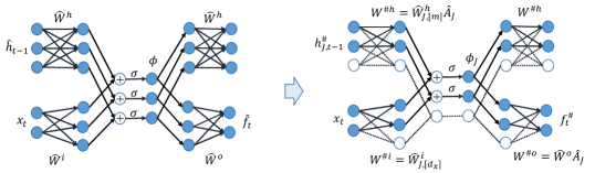
Figure 1: Spectral pruning for RNN

Remark 3.1.

In the case of the regularization parameter $\tau=0$, spectral pruning can be applied, but the following point must be noted. In this case, the uniqueness of the minimization problem of $\left\|\phi-A\phi_{J}\right\|^{2}_{n,T}$ with respect to $A$ does not generally hold (i.e., there might be several reconstruction matrices). One of the solutions is $\widehat{A}_{J}=\widehat{\Sigma}_{[m],J}\widehat{\Sigma}_{J,J}^{{\dagger}}$, which is the limit of (3.2) as $\tau\to 0$, where $\widehat{\Sigma}_{J,J}^{{\dagger}}$ is the pseudo-inverse of $\widehat{\Sigma}_{J,J}$. It should be noted that $\widehat{\Sigma}_{J,J}^{{\dagger}}$ coincides with the usual inverse $\widehat{\Sigma}_{J,J}^{-1}$, when $m^{\sharp}$ is smaller than or equal to the rank of the covariance matrix $\widehat{\Sigma}$.

Remark 3.2.

We consider the case of the regularization parameter $\tau=0$ and $m^{\sharp}\geq m_{\mathrm{nzr}}$, where $m_{\mathrm{nzr}}$ denotes the number of non-zero rows of $\widehat{\Sigma}$. Here, we would like to remark on the relation between $m_{\mathrm{nzr}}$ and pruning. Let $J_{\mathrm{nzr}}$ be the index set such that $[m]\setminus J_{\mathrm{nzr}}$ corresponds to zero rows of $\widehat{\Sigma}$. Then, by the definition (3.3) of $\widehat{\Sigma}$, we have for $i=1,\cdots,n$, $t=1,\cdots,T$, $v\in[m]\setminus J_{\mathrm{nzr}}$

$$\phi_{v}(x_{t}^{i},\widehat{h}^{i}_{t-1})=0,$$

which implies that $\widetilde{A}_{J_{\mathrm{nzr}}}=I_{[m],J_{\mathrm{nzr}}}$ is a trivial solution of the minimization problem because $\|\phi-\widetilde{A}_{J_{\mathrm{nzr}}}\phi_{J_{\mathrm{nzr}}}\|^{2}_{n,T}=0$. Here, $I_{[m],J_{\mathrm{nzr}}}$ is the submatrix of the identity matrix corresponding to the index sets $[m]$ and $J_{\mathrm{nzr}}$. If we choose $\widetilde{A}_{J_{\mathrm{nzr}}}=I_{[m],J_{\mathrm{nzr}}}$ as the reconstruction matrix, then the trivial compressed weights can be obtained by simply removing the columns corresponding to $[m]\setminus J_{\mathrm{nzr}}$, i.e., $W^{\sharp o}:=\widehat{W}^{o}\widetilde{A}_{J_{\mathrm{nzr}}}=\widehat{W}^{o}_{[m],J_{\mathrm{nzr}}}$ and $W^{\sharp h}:=\widehat{W}^{h}_{J_{\mathrm{nzr}},[m]}\widetilde{A}_{J_{\mathrm{nzr}}}=\widehat{W}^{h}_{J_{\mathrm{nzr}},J_{\mathrm{nzr}}}$, and its network $f^{\sharp}_{J_{\mathrm{nzr}}}$ coincides with the trained network $\widehat{f}$ for training data, i.e., for $i=1,\cdots,n$, $t=1,\cdots,T$

$$f^{\sharp}_{J_{\mathrm{nzr}},t}(X^{i}_{t})=\widehat{f}_{t}(X^{i}_{t})$$

which means that the trained RNN is compressed to size $m^{\sharp}$ without degradation. On the other hand, in the case of $m^{\sharp}<m_{\mathrm{nzr}}$, $\widetilde{A}_{J}=I_{[m],J}$ is not a solution of the minimization problem for any choice of the index $J$, which means that the compressed network using $\widehat{A}_{J}=\widehat{\Sigma}_{[m],J}\widehat{\Sigma}_{J,J}^{{\dagger}}$ is closer to the trained network than that using $\widetilde{A}_{J}=I_{[m],J}$. Therefore, spectral pruning essentially contributes to compression when $m^{\sharp}<m_{\mathrm{nzr}}$.

4 Generalization Error Bounds for Compressed RNNs

In this section, we discuss the generalization error bounds for compressed RNNs. In Subsection 4.1, the error bounds for general compressed RNNs are evaluated to explain the reason for deriving spectral pruning discussed in Section 3 in the error bound term. In Subsection 4.2, the error bounds for RNNs compressed with spectral pruning are evaluated.

4.1 Error bound for general compressed RNNs

Let $(X^{i}_{T},Y^{i}_{T})$ be the training data generated independently identically from the true distribution $P_{T}$, and let $f^{\sharp}$ be a general compressed RNN, and assume that it belongs to the following function space:

$$\begin{split}\mathcal{F}^{\sharp}_{T}&=\mathcal{F}^{\sharp}_{T}(R_{o},R_{h},R_{i},R^{b}_{o},R^{b}_{hi})\\ &:=\bigg{\{}f^{\sharp}\,\Big{|}\,f^{\sharp}(X_{T})=(f^{\sharp}_{t}(X_{t}))_{t=1}^{T},\\ &f^{\sharp}_{t}(X_{t})=(W^{\sharp o}\sigma(\cdot)+b^{\sharp o})\circ(W^{\sharp h}\sigma(\cdot)+W^{\sharp i}x_{t}+b^{\sharp hi})\circ\\ &\cdots\circ(W^{\sharp h}\sigma(\cdot)+W^{\sharp i}x_{2}+b^{\sharp hi})\circ(W^{\sharp i}x_{1}+b^{\sharp hi})\\ &\text{ for }X_{T}\in\mathrm{supp}(P_{X_{T}}),\ \big{\|}W^{\sharp o}\big{\|}_{F}\leq R_{o},\ \big{\|}W^{\sharp h}\big{\|}_{F}\leq R_{h},\\ &\big{\|}W^{\sharp i}\big{\|}_{F}\leq R_{i},\ \big{\|}b^{\sharp o}\big{\|}_{2}\leq R^{b}_{o},\ \big{\|}b^{\sharp hi}\big{\|}_{2}\leq R^{b}_{hi}\bigg{\}},\end{split}$$

where $P_{X_{T}}$ is the marginal distribution of $P_{T}$ with respect to $X_{T}$, and $R_{o}$, $R_{h}$, $R_{i}$, $R^{b}_{o}$, $R^{b}_{hi}$ are the upper bounds of the compressed weights $W^{\sharp o}\in\mathbb{R}^{d_{y}\times m^{\sharp}}$, $W^{\sharp h}\in\mathbb{R}^{m^{\sharp}\times m^{\sharp}}$, $W^{\sharp i}\in\mathbb{R}^{m^{\sharp}\times d_{x}}$, biases $b^{\sharp o}\in\mathbb{R}^{d_{y}}$, and $b^{\sharp hi}\in\mathbb{R}^{m^{\sharp}}$, respectively. Here, $\|\cdot\|_{F}$ denotes the Frobenius norm.

Assumption 4.1.

The following assumptions are made: (i) The marginal distribution $P_{x_{t}}$ of $P_{T}$ with respect to $x_{t}$ is bounded, i.e., there exist a constant $R_{x}$ independent of $t$ such that $\|x_{t}\|_{2}\leq R_{x}$ for all $x_{t}\in\mathrm{supp}(P_{x_{t}})$ and $t=1,\ldots,T.$ (ii) The activation function $\sigma:\mathbb{R}\to\mathbb{R}$ satisfies $\sigma(0)=0$ and $|\sigma(t)-\sigma(s)|\leq\rho_{\sigma}|t-s|$ for all $t,s\in\mathbb{R}.$

Under these assumptions, we obtain the following approximation error bounds between the trained network $\widehat{f}$ and compressed networks $f^{\sharp}$.

Proposition 4.2.

Let Assumption 4.1 hold. Let $(X_{T}^{1},Y_{T}^{1}),\ldots,(X_{T}^{n},Y_{T}^{n})$ be sampled i.i.d. from the distribution $P_{T}$. Then, for all $f^{\sharp}\in\mathcal{F}^{\sharp}_{T}$ and $J\subset[m]$ with $|J|=m^{\sharp}$, we have

$$\begin{split}&\big{\|}\widehat{f}-f^{\sharp}\big{\|}_{n,T}\leq\big{\|}\widehat{W}^{o}\phi-W^{\sharp o}\phi_{J}\big{\|}_{n,T}\\ +&\,\big{\|}\widehat{W}^{h}_{J,[m]}\phi-W^{\sharp h}\phi_{J}\big{\|}_{n,T}+\big{\|}\widehat{W}^{i}_{J,[d_{x}]}-W^{\sharp i}\big{\|}_{op}\\ +&\,\big{\|}\widehat{b}^{hi}_{J}-b^{\sharp hi}\big{\|}_{2}+\big{\|}\widehat{b}^{o}-b^{\sharp o}\big{\|}_{2}.\end{split}$$ (4.1)

Here, $\lesssim$ implies that the left-hand side in (4.1) is bounded above by the right-hand side times a constant independent of the trained weights and biases $\widehat{W}$, $\widehat{b}$ and compressed weights and biases $W^{\sharp}$, $b^{\sharp}$. The proof is given by direct computations. For the exact statement and proof, see Appendix B.

Remark 4.3.

Let $f^{\sharp}_{J}$ be the network compressed using the reconstruction matrix (see (iii) in Section 3). By applying Proposition 4.2 as $f^{\sharp}=f^{\sharp}_{J}$, we obtain

$$\begin{split}&\big{\|}\widehat{f}-f^{\sharp}_{J}\big{\|}^{2}_{n,T}\lesssim\underbrace{\big{\|}\widehat{W}^{o}\phi-\widehat{W}^{o}\widehat{A}_{J}\phi_{J}\big{\|}^{2}_{n,T}+\big{\|}\widehat{W}^{o}\widehat{A}_{J}\big{\|}^{2}_{\tau}}_{=L^{(B,o)}_{\tau}(J)}\\ &+\underbrace{\big{\|}\widehat{W}^{h}_{J,[m]}\phi-\widehat{W}^{h}_{J,[m]}\widehat{A}_{J}\phi_{J}\big{\|}^{2}_{n,T}+\big{\|}\widehat{W}^{h}_{J,[m]}\widehat{A}_{J}\big{\|}^{2}_{\tau}}_{=L^{(B,h)}_{\tau}(J)}\\ &\leq\left(\big{\|}\widehat{W}^{o}\big{\|}^{2}_{F}+\big{\|}\widehat{W}^{h}_{J,[m]}\big{\|}^{2}_{F}\right)\underbrace{\left(\big{\|}\phi-\widehat{A}_{J}\phi_{J}\big{\|}^{2}_{n,T}+\big{\|}\widehat{A}_{J}\big{\|}^{2}_{\tau}\right)}_{=L^{(A)}_{\tau}(J)},\end{split}$$ (4.2)

i.e., the approximation error is bounded above by the input information loss.

For the RNN $f=(f_{t})_{t=1}^{T}$, the training error with respect to the $j$-th component of the output is defined as

$$\widehat{\Psi}_{j}(f):=\frac{1}{nT}\sum_{i=1}^{n}\sum_{t=1}^{T}\psi(y^{i}_{t,j},f_{t}(X^{i}_{t})_{j}),$$

where $X_{t}=(x_{t})_{t=1}^{t}$ and $\psi:\mathbb{R}\times\mathbb{R}\to\mathbb{R}_{+}$ is a loss function. The generalization error with respect to the $j$-th component of the output is defined as

$$\Psi_{j}(f):=E\bigg{[}\frac{1}{T}\sum_{t=1}^{T}\psi(y_{t,j},f_{t}(X_{t})_{j})\bigg{]},$$

where the expectation is taken with respect to $(X_{T},Y_{T})\sim P_{T}$.

Assumption 4.4.

The following assumptions are made: (i) The loss function $\psi(y_{t,j},0)$ is bounded, i.e., there exists a constant $R_{y}$ such that $|\psi(y_{t,j},0)|\leq R_{y}$ for all $y_{t,j}\in\mathrm{supp}(P_{y_{t,j}})$, $t=1,\ldots,T$, $j=1,\ldots,d_{y}$. (ii) $\psi$ is $\rho_{\psi}$-Lipschitz continuous, i.e., $|\psi(y,f)-\psi(y,g)|\leq\rho_{\psi}|f-g|$ for all $y,f,g\in\mathbb{R}.$

We obtain the following generalization error bound for $f^{\sharp}\in\mathcal{F}_{T}^{\sharp}(R_{o},R_{h},R_{i},R^{b}_{o},R^{b}_{hi})$.

Theorem 4.5.

Let Assumptions 4.1 and 4.4 hold, and let $(X_{T}^{1},Y_{T}^{1}),\ldots,(X_{T}^{n},Y_{T}^{n})$ be sampled i.i.d. from the distribution $P_{T}$. Then, for any $\delta\geq\log 2$, we have the following inequality with probability greater than $1-2e^{-\delta}$:

$$\begin{split}&\Psi_{j}(f^{\sharp})\lesssim\widehat{\Psi}_{j}(\widehat{f})+\Big{\{}\big{\|}\widehat{W}^{o}\phi-W^{\sharp o}\phi_{J}\big{\|}_{n,T}\\ &+\big{\|}\widehat{W}^{h}_{J,[m]}\phi-W^{\sharp h}\phi_{J}\big{\|}_{n,T}+\big{\|}\widehat{W}^{i}_{J,[d_{x}]}-W^{\sharp i}\big{\|}_{op}\\ &+\big{\|}\widehat{b}^{hi}_{J}-b^{\sharp hi}\big{\|}_{2}+\big{\|}\widehat{b}^{o}-b^{\sharp o}\big{\|}_{2}\Big{\}}+\frac{1}{\sqrt{n}}(m^{\sharp})^{\frac{5}{4}}R^{1/2}_{\infty,T},\end{split}$$ (4.3)

for $j=1,\ldots,d_{y}$ and for all $J\subset[m]$ with $|J|=m^{\sharp}$, and $f^{\sharp}\in\mathcal{F}^{\sharp}_{T}$, where $R_{\infty,t}$ is defined by

$$R_{\infty,t}:=R_{o}\rho_{\sigma}(R_{i}R_{x}+R^{b}_{hi})\bigg{(}\sum_{l=1}^{t}(R_{h}\rho_{\sigma})^{l-1}\bigg{)}+R^{b}_{o}.$$

Here, $\lesssim$ implies that the left-hand side in (4.3) is bounded above by the right-hand side times a constant independent of the trained weights and biases $\widehat{W}$, $\widehat{b}$, compressed weights and biases $W^{\sharp}$, $b^{\sharp}$, compressed number $m^{\sharp}$, and the number of samples $n$. We remark that some omitted constants blow up as increasing $T$, but they can be controlled by increasing sampling number $n$ (see Theorem C.1). The idea behind the proof is that the generalization error is decomposed into the training, approximation, and estimation errors. The approximation and estimation errors are evaluated using Proposition 4.2 and the estimation of the Rademacher complexity, respectively. For the exact statement and proof, see Appendix C.

The second term in (4.3) is the approximation error bound between $\widehat{f}$ and $f^{\sharp}$ regarded as the bias, which is given by Proposition 4.1, while the third term is the estimation error bound regarded as the variance. It can be observed that minimizing the terms $\|\widehat{W}^{o}\phi-W^{\sharp o}\phi_{J}\|_{n,T}$ and $\|\widehat{W}^{h}_{J,[m]}\phi-W^{\sharp h}\phi_{J}\|_{n,T}$ with respect to $W^{\sharp o}$ and $W^{\sharp h}$ is equivalent to the output information losses (3.5) and (3.6) with $\tau=0$, respectively, which means that (iii) in Section 3 with $\tau=0$ constructs the compressed RNN such that the bias term becomes smaller. Considering $\tau\neq 0$ prevents the blow up of $\|W^{\sharp o}\|_{F}$ and $\|W^{\sharp h}\|_{F}$, which means that the regularization parameter $\tau$ plays an important role in preventing the blow up of the variance term because $R_{\infty,T}$ in the variance term includes the upper bounds $R_{o}$ and $R_{h}$ of $\|W^{\sharp o}\|_{F}$ and $\|W^{\sharp h}\|_{F}$. Therefore, (iii) with $\tau\neq 0$ constructs the compressed RNN such that the generalization error bound becomes smaller. In addition, selecting an optimal $J$ for minimizing the information losses (see (iv) in Section 3) further decreases the error bound.

4.2 Error bound for RNNs compressed with spectral pruning

Next, we evaluate the generalization error bounds for the RNN $f^{\sharp}_{J}$ compressed using the reconstruction matrix (see (iii) in Section 3). We define the degrees of freedom $\widehat{N}(\lambda)$ by

$$\widehat{N}(\lambda):=\mathrm{Tr}\big{[}\widehat{\Sigma}(\widehat{\Sigma}+\lambda I)^{-1}\big{]}=\sum_{j=1}^{m}\frac{\widehat{\mu}_{j}}{\widehat{\mu}_{j}+\lambda},$$

where $\widehat{\mu}_{j}$ is an eigenvalue of $\widehat{\Sigma}$. Throughout this subsection, the regularization parameter $\tau\in\mathbb{R}^{m^{\sharp}}_{+}$ is chosen as $\tau=\lambda m^{\sharp}\tau^{\prime}$, where $\lambda>0$ satisfies

$$m^{\sharp}\geq 5\widehat{N}(\lambda)\log(16\widehat{N}(\lambda)/\widetilde{\delta}),$$ (4.4)

for a prespecified $\widetilde{\delta}\in(0,1/2)$. Here, $\tau^{\prime}=(\tau^{\prime}_{j})_{j\in J}\in\mathbb{R}^{m^{\sharp}}$ is the leverage score defined by for $k\in[m]$

$$\tau^{\prime}_{k}:=\frac{1}{\widehat{N}(\lambda)}\big{[}\widehat{\Sigma}(\widehat{\Sigma}+\lambda I)^{-1}\big{]}_{k,k}=\frac{1}{\widehat{N}(\lambda)}\sum_{j=1}^{m}U^{2}_{k,j}\frac{\widehat{\mu}_{j}}{\widehat{\mu}_{j}+\lambda},$$ (4.5)

where $U=(U_{k,j})_{k,j}$ is the orthogonal matrix that diagonalizes $\widehat{\Sigma}$, i.e., $\widehat{\Sigma}=U\text{diag}\left\{\widehat{\mu}_{1},\ldots,\widehat{\mu}_{m}\right\}U^{T}$. The leverage score includes the information of the eigenvalues and eigenvectors of $\widehat{\Sigma}$, and indicates that the large components correspond to the important nodes from the viewpoint of the spectral information of $\widehat{\Sigma}$. Let $q$ be the probability measure on $[m]$ defined by

$$q(v):=\tau^{\prime}_{v}\quad\text{for}\ v\in[m].$$ (4.6)

Proposition 4.6.

Let $v_{1},\ldots,v_{m^{\sharp}}$ be sampled i.i.d. from the distribution $q$ in (4.6), and $J=\{v_{1},\ldots,v_{m^{\sharp}}\}$. Then, for any $\widetilde{\delta}\in(0,1/2)$ and $\lambda>0$ satisfying (4.4), we have the following inequality with probability greater than $1-\widetilde{\delta}$:

$$L^{(A)}_{\tau}(J)\leq 4\lambda.$$ (4.7)

The proof is given in Appendix E. In the proof, we essentially refer to previous work [(Bach). Combining (4.2) and (4.7), we conclude that

$$\big{\|}\widehat{f}-f^{\sharp}_{J}\big{\|}^{2}_{n,T}\lesssim\lambda.$$ (4.8)

It can be observed that the approximation error bound (4.8) is controlled by the degrees of freedom. If the eigenvalues of $\widehat{\Sigma}$ rapidly decrease, then $\widehat{N}(\lambda)$ is a rapidly decreasing function as $\lambda$ is large. Therefore, in that case, we can choose a smaller $\lambda$ even when $m^{\sharp}$ is fixed. We will numerically study the relationship between the eigenvalue distribution and the input information loss in Section 5.1.

We make the following additional assumption.

Assumption 4.7.

Assume that the upper bounds for the trained weights and biases are given by $\|\widehat{W}^{o}\|_{F}\leq\widehat{R}_{o}$, $\|\widehat{W}^{h}\|_{F}\leq\widehat{R}_{h}$, $\|\widehat{W}^{i}\|_{F}\leq\widehat{R}_{i}$, $\|\widehat{b}^{hi}\|_{2}\leq\widehat{R}^{b}_{hi}$, and $\|\widehat{b}^{o}\|_{2}\leq\widehat{R}^{b}_{o}$.

We have the following generalization error bound.

Theorem 4.8.

Let Assumptions 4.1, 4.4, and 4.7 hold, and let $(X_{T}^{1},Y_{T}^{1}),\ldots,(X_{T}^{n},Y_{T}^{n})$ and $v_{1},\ldots,v_{m^{\sharp}}$ be sampled i.i.d. from the distributions $P_{T}$ and $q$ in (4.6), respectively. Let $J=\{v_{1},\ldots,v_{m^{\sharp}}\}$. Then, for any $\delta\geq\log 2$ and $\widetilde{\delta}\in(0,1/2)$, we have the following inequality with probability greater than $(1-2e^{-\delta})\widetilde{\delta}$:

$$\Psi_{j}(f^{\sharp}_{J})\lesssim\widehat{\Psi}_{j}(\widehat{f})+\sqrt{\lambda}+\frac{1}{\sqrt{n}}(m^{\sharp})^{\frac{5}{4}},$$ (4.9)

for $j=1,\ldots,d_{y}$ and for all $\lambda>0$ satisfying (4.4).

Here, $\lesssim$ implies that the left-hand side in (4.9) is bounded above by the right-hand side times a constant independent of $\lambda$, $m^{\sharp}$, and $n$. We remark that some omitted constants blow up as increasing $T$, but they can be controlled by increasing sampling number $n$ (see Theorem F.1). The proof is given by the combination of applying Theorem 4.5 as $f^{\sharp}=f^{\sharp}_{J}$ and using Proposition 4.6. For the exact statement and proof, see Appendix F. It can be observed that in (4.9), a bias-variance tradeoff relationship exists with respect to $m^{\sharp}$. When $m^{\sharp}$ is large, $\lambda$ can be chosen smaller in the condition (4.4), which implies that the bias term (the second term in (4.9)) becomes smaller, but the variance term (the third term in (4.9)) becomes larger. In contrast, the bias becomes larger and the variance becomes smaller when $m^{\sharp}$ is small. Further remarks on Theorem 4.8 are given in Appendix G.

5 Numerical Experiments

In this section, numerical experiments are detailed to demonstrate our theoretical results and show the effectiveness of spectral pruning compared with existing methods. In Sections 5.1 and 5.2, we select the pixel-MNIST as our task and employ the IRNN, which is an RNN that uses the ReLU as the activation function and initializes weights as the identity matrix and biases to zero (see [(Le)). In Section 5.3, we select the PTB [(marcus1993building) and employ the RNNLM whose RNN layer is orthodox Elman-type. For RNN training details, see Appendix H. We choose parameters $\theta_{1}=1$, $\theta_{2}=\theta_{3}=0$ in (iv) of Section 3, i.e., we minimize only the input information loss. This choice is not so problematic because the bound of output information loss automatically becomes smaller with minimizing the input one (see Remark 4.3). We choose the regularization parameter $\tau=0$, where this choice regards $\widehat{f}$ as a well-trained network and gives priority to minimizing the approximation error between $\widehat{f}$ and $f^{\sharp}_{J}$ (see below Theorem4.5).

5.1 Eigenvalue distributions and information losses

First, we numerically study the relationship between the eigenvalue distribution and the information losses. Figure 2 shows the eigenvalue distribution of the covariance matrix $\widehat{\Sigma}$ with 128 hidden nodes, which are sorted in decreasing order. In this experiment, almost half of the eigenvalues are zero, which cannot be visualized in the figure. Figure 2 shows the input information loss $L^{(A)}_{0}(J)$ versus the compressed number $m^{\sharp}$. The information losses vanish when $m^{\sharp}>m_{\mathrm{nzr}}$ (see Remark 3.2). The blue and pink curves correspond to MNIST and FashionMNIST, respectively. It can be observed that the eigenvalues for MNIST decrease more rapidly than those for FashionMNIST, and the information losses for MNIST decrease more rapidly than those for FashionMNIST. This phenomenon coincides with the interpretation on Proposition 4.6 (see the discussion below (4.8)).

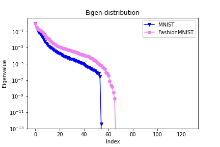
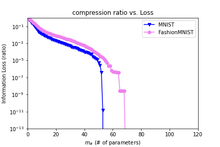
(a) Eigenvalue distribution for $\widehat{\Sigma}$           (b) Input information loss vs. $m^{\sharp}$

Figure 2: Relationship between the eigenvalue distribution and the input information loss

5.2 Pixel-MNIST (IRNN)

Table 1: Pixel-MNIST (IRNN)

Method	Accuracy[%] (std)	Finetuned Accuracy[%](std)	# input -hidden	# hidden -hidden	# hidden -out	total
Baseline(128)	96.80 (0.23)	-	128	16384	1280	17792
Baseline(42)	93.35 (0.75)	-	42	1764	420	2226
Spectral w/ rec.(ours)	92.61 (2.46)	97.08 (0.16)	42	1764	420	2226
Spectral w/o rec.	83.60 (8.24)	-	42	1764	420	2226
Random w/ rec.	34.72 (32.47)	-	42	1764	420	2226
Random w/o rec.	23.13 (16.09)	-	42	1764	420	2226
Random Weight	10.35 (1.38)	-	128	1764	1280	3172
Magnitude-based Weight	11.06 (0.70)	94.41 (3.02)	128	1764	1280	3172
Column Sparsification	84.80 (7.29)	-	128	5376	1280	6784
Low Rank Factorization	9.65 (3.85)	-	128	10752	1280	12160

Table 2: PTB (RNNLM)

Method	Perplexity (std)	Finetuned Perplexity (std)	# input -hidden	# hidden -hidden	# hidden -out	total
Baseline(128)	114.66 (0.35)	-	1270016	16384	1270016	2556416
Baseline(42)	145.85 (0.74)	132.46 (0.74)	416724	1764	416724	835212
Spectral w/ rec.(ours)	207.63 (2.19)	124.26 (0.39)	416724	1764	416724	835212
Spectral w/o rec.	433.99 (10.64)	-	416724	1764	416724	835212
Random w/ rec.	243.76 (9.46)	-	416724	1764	416724	835212
Random w/o rec.	492.06 (22.40)	-	416724	1764	416724	835212
Random Weight	203.41 (2.02)	-	1270016	1764	1270016	2541796
Magnitude-based Weight	168.57 (2.57)	115.65 (0.31)	1270016	1764	1270016	2541796
Magnitude-based Weight $\diamondsuit$	201.41 (3.60)	126.20 (0.28)	416724	1764	416724	835212
Column Sparsification	128.98 (0.52)	-	1270016	5376	1270016	2545408
Low Rank Factorization	126.24 (1.79)	-	1270016	10752	1270016	2550784

We compare spectral pruning with other pruning methods in the pixel-MNIST (IRNN). Table 1 summarizes the accuracies and the number of weight parameters for different pruning methods. We consider one-third compression in the hidden state, i.e., for the node pruning, 128 hidden nodes were compressed to 42 nodes, while for weight pruning, $128^{2}(=16384)$ hidden weights were compressed to $42^{2}(=1764)$ weights.

“Baseline(128)” and “Baseline(42)” represent direct training (not pruning) with 128 and 42 hidden nodes, respectively. “Spectral w/ rec.(ours)” represents spectral pruning with the reconstruction matrix (i.e., the compressed weight is chosen as $W^{\sharp h}=\widehat{W}^{h}_{J,[m]}\widehat{A}_{J}$ with the optimal $J$ with respect to (3.9)), while “Spectral w/o rec.” represents spectral pruning without the reconstruction matrix (i.e., $W^{\sharp h}=\widehat{W}^{h}_{J,J}$ with the optimal $J$ with respect to (3.9)), which idea is based on [(luo2017thinet). “Random w/ rec.” represents random node pruning with the reconstruction matrix (i.e., $W^{\sharp h}=\widehat{W}^{h}_{J,[m]}\widehat{A}_{J}$, where $J$ is randomly chosen), while “Random w/o rec.” represents random node pruning without the reconstruction matrix (i.e., $W^{\sharp h}=\widehat{W}^{h}_{J,J}$, where $J$ is randomly chosen). “Random Weight” represents random weight pruning. For the reason why we compare with random pruning, see the introduction of [(Zhang). “Magnitude-based Weight” represents magnitude-based weight pruning based on [(Narang). “Column Sparsification” represents the magnitude-based column sparsification during training based on [(wang2019acceleration). “Low Rank Factorization” represents low rank factorization which truncates small singular values of trained weights based on [(prabhavalkar2016compression). “Accuracy[%](std)” and “Finetuned Accuracy[%](std)” represent their mean (standard deviation) of accuracy before and after fine-tuning, respectively. “# input-hidden”, “# hidden-hidden”, and “# hidden-out” represent the number of input-to-hidden, hidden-to-hidden, and hidden-to-output weight parameters, respectively. “total” represents their sum. For detailed procedures of training, pruning, and fine-tuning, see Appendix H.

We demonstrate that spectral pruning significantly outperforms other pruning methods. The reason why spectral pruning can compress with small degradation is that the covariance matrix $\widehat{\Sigma}$ has a small number of non-zero rows (we observed around 50 non-zero rows). For the detail of non-zero rows, see Remark 3.2. Our method with fine-tuning outperforms “Baseline(42)”, which means that the spectral pruning gets benefits from over-parameterization [(chang2020provable; zhang2021understanding). Since the magnitude-based weight pruning is the method to require the fine-tuning (e.g., see [(Narang)), we have also compared our method with the magnitude-based weight pruning with fine-tuning, and observed that our method outperforms the magnitude-based weight pruning as well. We also remark that our method with fine-tuning overcomes “Baseline(128)”.

5.3 PTB (RNNLM)

We compare spectral pruning with other pruning methods in the PTB (RNNLM). Table 2 summarizes the perplexity and the number of weight parameters for different pruning methods. As in Section 5.2, we consider one-third compression in the hidden state, and how to represent “Method” is the same as Table 1 except for “Magnitude-based Weight $\diamondsuit$”, which represents the magnitude-based weight pruning for not only hidden-to-hidden weights but also input-to-hidden and hidden-to-out weights so that the number of resultant weight parameters is the same as Spectral w/ rec.(ours).

We demonstrate that our method with fine-tuning outperforms other pruning methods except for magnitude-based Weight pruning. Even though "Low Rank Factorization" retains large number of weight parameters, its perplexity is slightly worse than our method with fine-tuning. On the other hands, our method with fine-tuning can not outperform “Magnitude-based Weight”, but it can slightly do under the condition of the same number of weight parameters. We also remark that our method with fine-tuning overcomes “Baseline(42)”, although it does not overcome “Baseline(128)”.

Therefore, we conclude that spectral pruning works well in Elman-RNN, especially in IRNN.

Future Work

It would be interesting to extend our work to the long short-term memory (LSTM). The properties of LSTMs are different from those of RNNs in that LSTMs have the gated architectures including product operations, which might require more complicated analysis of the generalization error bounds as compared with RNNs. Hence, the investigation of spectral pruning for LSTMs is beyond the scope of this study and will be the focus of future work.

Acknowledgements

The authors are grateful to Professor Taiji Suzuki for useful discussions and comments on our work. The first author was supported by Grant-in-Aid for JSPS Fellows (No.21J00119), Japan Society for the Promotion of Science.

Appendix

Appendix A Review of Spectral Pruning for DNNs

Let $D=\{(x^{i},y^{i})\}_{i=1}^{n}$ be training data, where $x^{i}\in\mathbb{R}^{d_{x}}$ is an input and $y^{i}\in\mathbb{R}^{d_{y}}$ is an output. The training data are independently identically distributed. To train the appropriate relationship between input and output, we consider DNNs $f$ as

$$f(x)=(W^{(L)}\sigma(\cdot)+b^{(L)})\circ\cdots\circ(W^{(1)}x+b^{(1)}),$$

where $\sigma:\mathbb{R}\to\mathbb{R}$ is an activation function, $W^{(l)}\in\mathbb{R}^{m_{l+1}\times m_{l}}$ is a weight matrix, and $b^{(l)}\in\mathbb{R}^{m_{l+1}}$ is a bias. Let $\widehat{f}$ be a trained DNN obtained from the training data $D$, i.e.,

$$\widehat{f}(x)=(\widehat{W}^{(L)}\sigma(\cdot)+\widehat{b}^{(L)})\circ\cdots\circ(\widehat{W}^{(1)}x+\widehat{b}^{(1)}).$$

We denote the input with respect to $l$-th layer by

$$\phi^{(l)}(x)=\sigma\circ(\widehat{W}^{(l-1)}\sigma(\cdot)+\widehat{b}^{(l-1)})\circ\cdots\circ(\widehat{W}^{(1)}x+\widehat{b}^{(1)}).$$

Let $J^{(l)}\subset[m_{l}]$ be an index set with $|J^{(l)}|=m^{\sharp}_{l}$, where $[m_{l}]:=\{1,\ldots,m_{l}\}$ and $m^{\sharp}_{l}\in\mathbb{N}$ is the number of nodes of the $l$-th layer of the compressed DNN $f^{\sharp}$ with $m^{\sharp}_{l}\leq m_{l}$. Let $\phi^{(l)}_{J^{(l)}}(x)=(\phi^{(l)}_{j}(x))_{j\in J^{(l)}}$ be a subvector of $\phi^{(l)}(x)$ corresponding to the index set $J^{(l)}$, where $\phi^{(l)}_{j}(x)$ is the $j$-th components of the vector $\phi^{(l)}(x)$.

(i) Input information loss. The input information loss is defined by

$$L^{(A,l)}_{\tau}(J^{(l)}):=\min_{A\in\mathbb{R}^{m_{l}\times m^{\sharp}_{l}}}\big{\{}\big{\|}\phi^{(l)}-A\phi^{(l)}_{J^{(l)}}\big{\|}^{2}_{n}+\big{\|}A\big{\|}^{2}_{\tau}\big{\}},$$ (A.1)

where $\|\cdot\|_{n}$ is the empirical $L^{2}$-norm with respect to $n$, i.e.,

$$\big{\|}\phi^{(l)}-A\phi^{(l)}_{J^{(l)}}\big{\|}^{2}_{n}:=\frac{1}{n}\sum_{i=1}^{n}\big{\|}\phi^{(l)}(x^{i})-A\phi^{(l)}_{J^{(l)}}(x^{i})\big{\|}^{2}_{2},$$ (A.2)

where $\|\cdot\|_{2}$ is the Euclidean norm and $\|A\|^{2}_{\tau}:=\mathrm{Tr}\,[AI_{\tau}A^{T}]$ for a regularization parameter $\tau\in\mathbb{R}^{m^{\sharp}_{l}}_{+}$. Here, $\mathbb{R}^{m^{\sharp}_{l}}_{+}:=\big{\{}x\in\mathbb{R}^{m^{\sharp}_{l}}\,|\,x_{j}>0,\ j=1,\ldots,m^{\sharp}_{l}\big{\}}$ and $I_{\tau}:=\text{diag}(\tau)$. By the linear regularization theory, there exists a unique solution $\widehat{A}^{(l)}_{J^{(l)}}\in\mathbb{R}^{m_{l}\times m^{\sharp}_{l}}$ of the minimization problem of $\|\phi^{(l)}-A\phi^{(l)}_{J^{(l)}}\|^{2}_{n}+\|A\|^{2}_{\tau}$, and it has the form

$$\widehat{A}^{(l)}_{J^{(l)}}=\widehat{\Sigma}^{(l)}_{[m_{l}],J^{(l)}}\big{(}\widehat{\Sigma}^{(l)}_{J^{(l)},J^{(l)}}+I_{\tau}\big{)}^{-1},$$ (A.3)

where $\widehat{\Sigma}^{(l)}$ is the (noncentered) empirical covariance matrix of $\phi^{(l)}(x)$ with respect to $n$, i.e.,

$$\widehat{\Sigma}^{(l)}=\frac{1}{n}\sum_{i=1}^{n}\phi^{(l)}(x^{i})\phi^{(l)}(x^{i})^{T},$$

and $\widehat{\Sigma}^{(l)}_{I,I^{\prime}}=(\widehat{\Sigma}^{(l)}_{i,i^{\prime}})_{i\in I,i^{\prime}\in I^{\prime}}\in\mathbb{R}^{K\times H}$ is the submatrix of $\widehat{\Sigma}^{(l)}$ corresponding to index sets $I,I^{\prime}\subset[m]$ with $|I|=K$ and $|I^{\prime}|=H$. By substituting the explicit formula (A.2) of the reconstruction matrix $\widehat{A}^{(l)}_{J^{(l)}}$ into (A.1), the input information loss is reformulated as

$$L^{(A,l)}_{\tau}(J^{(l)})=\mathrm{Tr}\Big{[}\widehat{\Sigma}^{(l)}-\widehat{\Sigma}^{(l)}_{[m_{l}],J^{(l)}}\big{(}\widehat{\Sigma}^{(l)}_{J^{(l)},J^{(l)}}+I_{\tau}\big{)}^{-1}\widehat{\Sigma}^{(l)}_{J^{(l)},[m_{l}]}\Big{]}.$$ (A.4)

(ii) Output information loss. For any matrix $Z^{(l)}\in\mathbb{R}^{m\times m_{l}}$ with an output size $m\in\mathbb{N}$, we define the output information loss by

$$L^{(B,l)}_{\tau}(J^{(l)}):=\sum_{j=1}^{m}\min_{\beta\in\mathbb{R}^{m_{l}^{\sharp}}}\big{\{}\big{\|}Z^{(l)}_{j,:}\phi^{(l)}-\beta^{T}\phi^{(l)}_{J^{(l)}}\big{\|}^{2}_{n}+\big{\|}\beta^{T}\big{\|}^{2}_{\tau}\big{\}},$$ (A.5)

where $Z^{(l)}_{j,:}$ denotes the $j$-th row of the matrix $Z^{(l)}$. A typical situation is that $Z^{(l)}=\widehat{W}^{(l)}$. The minimization problem of $\|Z^{(l)}_{j,:}\phi^{(l)}-\beta^{T}\phi_{J^{(l)}}\|^{2}_{n}$ $+$ $\|\beta^{T}\|^{2}_{\tau}$ has the unique solution

$$\widehat{\beta}^{(l)}_{j}=(Z^{(l)}_{j,:}\widehat{A}^{(l)}_{J^{(l)}})^{T},$$

and by substituting it into (A.5), the output information loss is reformulated as

$$L^{(B,l)}_{\tau}(J^{(l)})=\mathrm{Tr}\Big{[}Z^{(l)}\big{(}\widehat{\Sigma}^{(l)}-\widehat{\Sigma}^{(l)}_{[m],J^{(l)}}\big{(}\widehat{\Sigma}^{(l)}_{J^{(l)},J^{(l)}}+I_{\tau}\big{)}^{-1}\widehat{\Sigma}^{(l)}_{J^{(l)},[m]}\big{)}Z^{(l)T}\Big{]}.$$

(iii) Compressed DNN by the reconstruction matrix. We construct the compressed DNN by

$$f^{\sharp}_{J^{(1:L)}}(x)=(W^{\sharp(L)}_{J^{(L)}}\sigma(\cdot)+b^{\sharp(L)})\circ\cdots\circ(W^{\sharp(1)}_{J^{(1)}}x+b^{\sharp(1)}),$$

where $J^{(1:L)}=J^{(1)}\cup\cdots\cup J^{(L)}$, and $b^{\sharp(l)}=\widehat{b}^{(l)}$ and $W^{\sharp(l)}_{J^{(l)}}$ is the compressed weight as the multiplication of the trained weight $\widehat{W}^{(l)}_{J^{(l+1)},[m_{l}]}$ and the reconstruction matrix $\widehat{A}_{J^{(l)}}$, i.e.,

$$W^{\sharp(l)}_{J^{(l)}}:=\widehat{W}^{(l)}_{J^{(l+1)},[m_{l}]}\widehat{A}_{J^{(l)}}.$$ (A.6)

.

(iv) Optimization. To select an appropriate index set $J^{(l)}$, we consider the following optimization problem that minimizes a convex combination of input and output information losses, i.e.,

$$\min_{J^{(l)}\subset[m_{l}]\ s.t.\ |J^{(l)}|=m^{\sharp}_{l}}\big{\{}\theta L^{(A,l)}_{\tau}(J^{(l)})+(1-\theta)L^{(B,l)}_{\tau}(J^{(l)})\big{\}},$$

for $\theta\in[0,1]$, where $m^{\sharp}_{l}\in[m]$ is a prespecified number. We adapt the optimal index $J^{\sharp(1:L)}$ in the algorithm. We term this method as spectral pruning.

In [[Suzuki], the generalization error bounds for compressed DNNs with the spectral pruning have been studied (see Theorems 1 and 2 in [[Suzuki]), and the parameters $\theta$, $\tau$, and $Z^{(l)}$ are chosen such that its error bound become smaller.

Appendix B Proof of Proposition 4.2

We restate Proposition 4.2 in an exact form as follows:

Proposition B.1.

Suppose that Assumption 4.1 holds. Let $\{(X_{T}^{i},Y_{T}^{i})\}_{i=1}^{n}$ be sampled i.i.d. from the distribution $P_{T}$. Then,

$$\|\widehat{f}-f^{\sharp}\|_{n,T}\leq\sqrt{3}\,\biggl{\{}\big{\|}\widehat{W}^{o}\phi-W^{\sharp o}\phi_{J}\big{\|}_{n,T}+R_{o}\rho_{\sigma}\max\{1,(R_{h}\rho_{\sigma})^{T-2}\}T\big{\|}\widehat{W}^{h}_{J,[m]}\phi-W^{\sharp h}\phi_{J}\big{\|}_{n,T}\\ +R_{o}\rho_{\sigma}\bigg{(}\sum_{t=1}^{T}(R_{h}\rho_{\sigma})^{t-1}\bigg{)}\big{(}R_{x}\big{\|}\widehat{W}^{i}_{J,[d_{x}]}-W^{\sharp i}\big{\|}_{op}+\|\widehat{b}^{hi}_{J}-b^{\sharp hi}\|_{2}\big{)}+\big{\|}\widehat{b}^{o}-b^{\sharp o}\big{\|}_{2}\biggr{\}},$$ (B.1)

for all $f^{\sharp}\in\mathcal{F}^{\sharp}_{T}(R_{o},R_{h},R_{i},R^{b}_{o},R^{b}_{hi})$ and $J\subset[m]$ with $|J|=m^{\sharp}$.

Proof.

Let $\widehat{f}=(\widehat{f}_{t})_{t=1}^{T}$ be a trained RNN and $f^{\sharp}\in\mathcal{F}^{\sharp}_{T}(R_{o},R_{h},R_{i},R^{b}_{o},R^{b}_{hi})$. Let us define functions $\phi$ and $\phi^{\sharp}$ by

$$\phi(x,h):=\sigma(\widehat{W}^{h}h+\widehat{W}^{i}x+\widehat{b}^{hi})\quad\text{for}\ x\in\mathbb{R}^{d_{x}},\ h\in\mathbb{R}^{m},$$

$$\phi^{\sharp}(x,h^{\sharp}):=\sigma(W^{\sharp h}h^{\sharp}+W^{\sharp i}x+b^{\sharp hi})\quad\text{for}\ x\in\mathbb{R}^{d_{x}},\ h^{\sharp}\in\mathbb{R}^{m^{\sharp}},$$ (B.2)

and denote the hidden states by

$$\widehat{h}_{t}:=\phi(x_{t},\widehat{h}_{t-1}),\ \ h^{\sharp}_{t}:=\phi^{\sharp}(x_{t},h^{\sharp}_{t-1})\quad\text{for}\ t=1,2,\cdots,T.$$ (B.3)

If a training data $X^{i}_{T}=(x^{i}_{t})_{t=1}^{T}$ is used as input, we denote its hidden states by

$$\widehat{h}^{i}_{t}:=\phi(x^{i}_{t},\widehat{h}^{i}_{t-1}),\ \ h^{\sharp i}_{t}:=\phi^{\sharp}(x^{i}_{t},h^{\sharp i}_{t-1}),$$

and its outputs at time $t$ by

$$\widehat{f}_{t}(X^{i}_{t})=\widehat{W}^{o}\phi(x^{i}_{t},\widehat{h}^{i}_{t-1})+\widehat{b}^{o},\quad f^{\sharp}_{t}(X^{i}_{t})=W^{\sharp o}\phi^{\sharp}(x^{i}_{t},h^{\sharp i}_{t-1})+b^{\sharp o},$$

for $t=1,2,\ldots,T$. Then, we have

$$\begin{split}\big{\|}\widehat{f}_{t}(X^{i}_{t})-f^{\sharp}_{t}(X^{i}_{t})\big{\|}_{2}&\leq\big{\|}\widehat{W}^{o}\phi(x^{i}_{t},\widehat{h}^{i}_{t-1})-W^{\sharp o}\phi_{J}(x^{i}_{t},\widehat{h}^{i}_{t-1})\big{\|}_{2}\\ &+\big{\|}W^{\sharp o}\phi_{J}(x^{i}_{t},\widehat{h}^{i}_{t-1})-W^{\sharp o}\phi^{\sharp}(x^{i}_{t},h^{\sharp i}_{t-1})\big{\|}_{2}+\big{\|}\widehat{b}^{o}-b^{\sharp o}\big{\|}_{2}.\end{split}$$ (B.4)

If we can prove that the second term of right-hand side in (B.4) is estimated as

$$\big{\|}W^{\sharp o}\phi_{J}(x^{i}_{t},\widehat{h}^{i}_{t-1})-W^{\sharp o}\phi^{\sharp}(x^{i}_{t},h^{\sharp i}_{t-1})\big{\|}_{2}\\ \leq R_{o}\rho_{\sigma}\bigg{\{}\max\big{\{}1,(R_{h}\rho_{\sigma})^{t-2}\big{\}}\sum_{l=1}^{t-1}\big{\|}\widehat{W}^{h}_{J,[m]}\phi(x^{i}_{t-l},\widehat{h}^{i}_{t-l-1})-W^{\sharp h}\phi_{J}(x^{i}_{t-l},\widehat{h}^{i}_{t-l-1})\big{\|}_{2}\\ +\sum_{l=1}^{t}(R_{h}\rho_{\sigma})^{l-1}\big{(}\big{\|}\widehat{W}^{i}_{J,[d_{x}]}-W^{\sharp i}\big{\|}_{op}\|x^{i}_{t-l+1}\|_{2}+\big{\|}\widehat{b}^{hi}_{J}-b^{\sharp hi}\big{\|}_{2}\big{)}\bigg{\}},$$ (B.5)

then by using the inequalities (B.4) and $(\sum_{k=1}^{K}a_{k})^{2}\leq K\sum_{k=1}^{K}a_{k}^{2}$, we have

$$\begin{split}&\big{\|}\widehat{f}_{t}(X^{i}_{t})-f^{\sharp}_{t}(X^{i}_{t})\big{\|}_{2}^{2}\leq 3\Bigg{\{}\big{\|}\widehat{W}^{o}\phi(x^{i}_{t},\widehat{h}^{i}_{t-1})-W^{\sharp o}\phi_{J}(x^{i}_{t},\widehat{h}^{i}_{t-1})\big{\|}_{2}^{2}\\ &+\bigg{(}R_{o}\rho_{\sigma}\max\big{\{}1,(R_{h}\rho_{\sigma})^{t-2}\big{\}}\sum_{l=1}^{t-1}\big{\|}\widehat{W}^{h}_{J,[m]}\phi(x^{i}_{t-l},\widehat{h}^{i}_{t-l-1})-W^{\sharp h}\phi_{J}(x^{i}_{t-l},\widehat{h}^{i}_{t-l-1})\big{\|}_{2}\bigg{)}^{2}\\ &+\bigg{(}R_{o}\rho_{\sigma}\sum_{l=1}^{t}(R_{h}\rho_{\sigma})^{l-1}\big{(}\big{\|}\widehat{W}^{i}_{J,[d_{x}]}-W^{\sharp i}\big{\|}_{op}\|x^{i}_{t-l+1}\|_{2}+\big{\|}\widehat{b}^{hi}_{J}-b^{\sharp hi}\big{\|}_{2}\big{)}+\big{\|}\widehat{b}^{o}-b^{\sharp o}\big{\|}_{2}\bigg{)}^{2}\Bigg{\}}.\end{split}$$

Hence, by taking the average over $i=1,\ldots,n$ and $t=1,\ldots,T$, and by using the inequality $\sum_{t=1}^{T}(\sum_{l=1}^{t}a_{l})^{2}\leq T^{2}\sum_{t=1}^{T}a_{t}^{2}$, we obtain

$$\begin{split}&\big{\|}\widehat{f}-f^{\sharp}\big{\|}_{n,T}^{2}=\frac{1}{nT}\sum_{i=1}^{n}\sum_{t=1}^{T}\big{\|}\widehat{f}_{t}(X^{i}_{t})-f^{\sharp}_{t}(X^{i}_{t})\big{\|}^{2}_{2}\\ &\leq 3\,\Bigg{\{}\underbrace{\frac{1}{nT}\sum_{i=1}^{n}\sum_{t=1}^{T}\big{\|}\widehat{W}^{o}\phi(x^{i}_{t},\widehat{h}^{i}_{t-1})-W^{\sharp o}\phi_{J}(x^{i}_{t},\widehat{h}^{i}_{t-1})\big{\|}_{2}^{2}}_{=\|\widehat{W}^{o}\phi-W^{\sharp o}\phi_{J}\|_{n,T}^{2}}\\ &+\big{(}R_{o}\rho_{\sigma}\max\big{\{}1,(R_{h}\rho_{\sigma})^{T-2}\big{\}}T\big{)}^{2}\underbrace{\frac{1}{nT}\sum_{i=1}^{n}\sum_{t=1}^{T}\big{\|}\widehat{W}^{h}_{J,[m]}\phi(x^{i}_{t},\widehat{h}^{i}_{t-1})-W^{\sharp h}\phi_{J}(x^{i}_{t},\widehat{h}^{i}_{t-1})\big{\|}_{2}^{2}}_{=\|\widehat{W}^{h}_{J,[m]}\phi-W^{\sharp h}\phi_{J}\|_{n,T}^{2}}\\ &+\bigg{(}R_{o}\rho_{\sigma}\bigg{(}\sum_{t=1}^{T}(R_{h}\rho_{\sigma})^{t-1}\bigg{)}\big{(}\big{\|}\widehat{W}^{i}_{J,[d_{x}]}-W^{\sharp i}\big{\|}_{op}\|x^{i}_{t-l+1}\|_{2}+\big{\|}\widehat{b}^{hi}_{J}-b^{\sharp hi}\big{\|}_{2}\big{)}+\big{\|}\widehat{b}^{o}-b^{\sharp o}\big{\|}_{2}^{2}\bigg{)}^{2}\Bigg{\}},\end{split}$$

which concludes the inequality (B.1). It remains to prove (B.5). We calculate that

$$\begin{split}\big{\|}W^{\sharp o}\phi_{J}(x^{i}_{t},&\,\widehat{h}^{i}_{t-1})-W^{\sharp o}\phi^{\sharp}(x^{i}_{t},h^{\sharp i}_{t-1})\big{\|}_{2}\\ &\leq\big{\|}W^{\sharp o}\big{\|}_{op}\big{\|}\sigma\big{(}\widehat{W}^{h}_{J,[m]}\phi(x^{i}_{t-1},\widehat{h}^{i}_{t-2})+\widehat{W}^{i}_{J,[d_{x}]}x^{i}_{t}+\widehat{b}^{hi}_{J}\big{)}\\ &\hskip 113.81102pt-\sigma\big{(}W^{\sharp h}\phi^{\sharp}(x^{i}_{t-1},h^{\sharp i}_{t-2})+W^{\sharp i}x^{i}_{t}+b^{\sharp hi}\big{)}\big{\|}_{2}\\ &\leq R_{o}\rho_{\sigma}\bigg{\{}\underbrace{\big{\|}\widehat{W}^{h}_{J,[m]}\phi(x^{i}_{t-1},\widehat{h}^{i}_{t-2})-W^{\sharp h}\phi^{\sharp}(x^{i}_{t-1},h^{\sharp i}_{t-2})\big{\|}_{2}}_{=:H_{t-1}}\\ &\hskip 113.81102pt+\big{\|}\widehat{W}^{i}_{J,[d_{x}]}-W^{\sharp i}\big{\|}_{op}\|x^{i}_{t}\|_{2}+\big{\|}\widehat{b}^{hi}-b^{\sharp hi}\big{\|}_{2}\bigg{\}},\end{split}$$ (B.6)

where $\|\cdot\|_{op}$ is the operator norm (which is the largest singular value). Concerning the quantity $H_{t-1}$, we estimate

$$H_{t-1}\leq\big{\|}\widehat{W}^{h}_{J,[m]}\phi(x^{i}_{t-1},\widehat{h}^{i}_{t-2})-W^{\sharp h}\phi_{J}(x^{i}_{t-1},\widehat{h}^{i}_{t-2})\big{\|}_{2}\\ +\big{\|}W^{\sharp h}\phi_{J}(x^{i}_{t-1},\widehat{h}^{i}_{t-2})-W^{\sharp h}\phi^{\sharp}(x^{i}_{t-1},h^{\sharp i}_{t-2})\big{\|}_{2},$$

and moreover, the second term is estimated as

$$\begin{split}\big{\|}W^{\sharp h}\phi_{J}(x^{i}_{t-1},&\,\widehat{h}^{i}_{t-2})-W^{\sharp h}\phi^{\sharp}(x^{i}_{t-1},h^{\sharp i}_{t-2})\big{\|}_{2}\\ &\leq\big{\|}W^{\sharp h}\big{\|}_{op}\big{\|}\sigma\big{(}\widehat{W}^{h}_{J,[m]}\phi(x^{i}_{t-2},\widehat{h}^{i}_{t-3})+\widehat{W}^{i}_{J,[d_{x}]}x^{i}_{t-1}+\widehat{b}^{hi}_{J}\big{)}\\ &\quad\quad\quad\quad\quad\quad\quad\quad\quad\quad\quad-\sigma\big{(}W^{\sharp h}\phi^{\sharp}(x^{i}_{t-2},h^{\sharp i}_{t-3})+W^{\sharp i}x^{i}_{t-1}+b^{\sharp hi}\big{)}\big{\|}_{2}\\ &\leq R_{h}\rho_{\sigma}\Big{\{}H_{t-2}+\big{\|}\widehat{W}^{i}_{J,[d_{x}]}-W^{\sharp i}\big{\|}_{op}\|x^{i}_{t-1}\|_{2}+\big{\|}\widehat{b}^{hi}_{J}-b^{\sharp hi}\big{\|}_{2}\Big{\}},\end{split}$$

for all $t$. Thus, we have the recursive inequality

$$\begin{split}H_{t-1}&\leq\big{\|}\widehat{W}^{h}_{J,[m]}\phi(x^{i}_{t-1},\widehat{h}^{i}_{t-2})-W^{\sharp h}\phi_{J}(x^{i}_{t-1},\widehat{h}^{i}_{t-2})\big{\|}_{2}\\ &\quad+R_{h}\rho_{\sigma}\Big{\{}H_{t-2}+\big{\|}\widehat{W}^{i}_{J,[d_{x}]}-W^{\sharp i}\big{\|}_{op}\|x^{i}_{t-1}\|_{2}+\big{\|}\widehat{b}^{hi}_{J}-b^{\sharp hi}\big{\|}_{2}\Big{\}},\end{split}$$ (B.7)

for $t=2,\ldots,T$. By repeatedly substituting (B.7) into (B.6), we arrive at (B.5):

$$\begin{split}\big{\|}W^{\sharp o}&\,\phi_{J}(x^{i}_{t},\widehat{h}^{i}_{t-1})-W^{\sharp o}\phi^{\sharp}(x^{i}_{t},h^{\sharp i}_{t-1})\big{\|}_{2}\\ &\leq R_{o}\rho_{\sigma}\bigg{\{}\sum_{l=1}^{t-1}\underbrace{(R_{h}\rho_{\sigma})^{l-1}}_{\leq\,\max\{1,(R_{h}\rho_{\sigma})^{t-2}\}}\big{\|}\widehat{W}^{h}_{J,[m]}\phi(x^{i}_{t-l},\widehat{h}^{i}_{t-l-1})-W^{\sharp h}\phi_{J}(x^{i}_{t-l},\widehat{h}^{i}_{t-l-1})\big{\|}_{2}\\ &\quad+\sum_{l=1}^{t}(R_{h}\rho_{\sigma})^{l-1}\big{(}\big{\|}\widehat{W}^{i}_{J,[d_{x}]}-W^{\sharp i}\big{\|}_{op}\|x^{i}_{t-l+1}\|_{2}+\big{\|}\widehat{b}^{hi}_{J}-b^{\sharp hi}\big{\|}_{2}\big{)}\bigg{\}}.\end{split}$$

Thus, we conclude Proposition B.1. ∎

Appendix C Proof of Theorem 4.5

We restate Theorem 4.5 in an exact form as follows:

Theorem C.1.

Suppose that Assumptions 4.1 and 4.4 hold. Let $\{(X_{T}^{i},Y_{T}^{i})\}_{i=1}^{n}$ be sampled i.i.d. from the distribution $P_{T}$. Then, for any $\delta\geq\log 2$, we have the following inequality with probability greater than $1-2e^{-\delta}$:

$$\begin{split}\Psi_{j}(f^{\sharp})&\leq\widehat{\Psi}_{j}(\widehat{f})+\sqrt{3}\rho_{\psi}\Bigg{\{}\big{\|}\widehat{W}^{o}\phi-W^{\sharp o}\phi_{J}\big{\|}_{n,T}\\ &\quad+R_{o}\rho_{\sigma}\max\{1,(R_{h}\rho_{\sigma})^{T-2}\}T\big{\|}\widehat{W}^{h}_{J,[m]}\phi-W^{\sharp h}\phi_{J}\big{\|}_{n,T}\\ &\quad+R_{o}\rho_{\sigma}\bigg{(}\sum_{t=1}^{T}(R_{h}\rho_{\sigma})^{t-1}\bigg{)}\big{(}R_{x}\big{\|}\widehat{W}^{i}_{J,[d_{x}]}-W^{\sharp i}\big{\|}_{op}+\big{\|}\widehat{b}^{hi}_{J}-b^{\sharp hi}\big{\|}_{2}\big{)}+\big{\|}\widehat{b}^{o}-b^{\sharp o}\big{\|}_{2}\Bigg{\}}\\ &\quad+\frac{1}{\sqrt{n}}\Bigg{\{}\frac{\widehat{c}\rho_{\psi}\sqrt{m^{\sharp}}}{T}\bigg{(}\sum_{t=1}^{T}M_{t}^{1/2}R^{1/2}_{\infty,t}\bigg{)}+3\sqrt{2\delta}(\rho_{\psi}R_{\infty,T}+R_{y})\Bigg{\}},\end{split}$$

for $j=1,\ldots,d_{y}$ and for all $J\subset[m]$ with $|J|=m^{\sharp}$ and $f^{\sharp}\in\mathcal{F}^{\sharp}_{T}(R_{o},R_{h},R_{i},R^{b}_{o},R^{b}_{hi})$, where $\widehat{c}:=192\sqrt{5}$, and $R_{\infty,t}$ and $M_{t}$ are defined by

$$R_{\infty,t}:=R_{o}\rho_{\sigma}(R_{i}R_{x}+R^{b}_{hi})\bigg{(}\sum_{l=1}^{t}(R_{h}\rho_{\sigma})^{l-1}\bigg{)}+R^{b}_{o},$$ (C.1)

$$\begin{split}M_{t}&:=R_{o}\rho_{\sigma}\biggl{[}\big{(}d_{y}\min\{\sqrt{m^{\sharp}},\sqrt{d_{y}}\}+d_{x}\min\{\sqrt{m^{\sharp}},\sqrt{d_{x}}\}\big{)}R_{i}R_{x}\\ &\quad+\big{(}d_{y}\min\{\sqrt{m^{\sharp}},\sqrt{d_{y}}\}+1\big{)}R^{b}_{hi}\biggr{]}\bigg{(}\sum_{l=0}^{t-1}(R_{h}\rho_{\sigma})^{l}\bigg{)}\\ &\quad+(m^{\sharp})^{\frac{3}{2}}R_{h}\rho_{\sigma}^{2}R_{o}(R_{i}R_{x}+R^{b}_{hi})\bigg{(}\sum_{l=1}^{t-1}\sum_{k=0}^{l-1}(R_{h}\rho_{\sigma})^{t-1-l+k}\bigg{)}+d_{y}R^{b}_{o}.\end{split}$$ (C.2)

Proof.

The generalization error of $f^{\sharp}_{t}\in\mathcal{F}^{\sharp}_{t}$ is decomposed into

$$\Psi_{j}(f^{\sharp})=\Psi_{j}(\widehat{f})+\big{(}\widehat{\Psi}_{j}(f^{\sharp})-\widehat{\Psi}_{j}(\widehat{f})\big{)}+\big{(}\Psi_{j}(f^{\sharp})-\widehat{\Psi}_{j}(f^{\sharp})\big{)},$$

where the second term $\widehat{\Psi}_{j}(f^{\sharp})-\widehat{\Psi}_{j}(\widehat{f})$ is called the approximation error and the third term $\Psi_{j}(f^{\sharp})-\widehat{\Psi}_{j}(f^{\sharp})$ is called the estimation error. Since the loss function $\psi$ is $\rho_{\psi}$-Lipschitz continuous, the approximation error is evaluated as

$$\begin{split}\big{|}\widehat{\Psi}_{j}(f^{\sharp})-\widehat{\Psi}_{j}(\widehat{f})\big{|}&\leq\frac{1}{nT}\sum_{i=1}^{n}\sum_{t=1}^{T}\big{|}\psi(y^{i}_{t,j},f^{\sharp}_{t}(X^{i}_{t})_{j})-\psi(y^{i}_{t},\widehat{f}_{t}(X^{i}_{t})_{j})\big{|}\\ &\leq\frac{\rho_{\psi}}{nT}\sum_{i=1}^{n}\sum_{t=1}^{T}\big{|}f^{\sharp}(X^{i}_{t})_{j}-\widehat{f}_{t}(X^{i}_{t})_{j}\big{|}\\ &\leq\frac{\rho_{\psi}}{nT}\sum_{i=1}^{n}\sum_{t=1}^{T}\big{\|}f^{\sharp}_{t}(X^{i}_{t})-\widehat{f}_{t}(X^{i}_{t})\big{\|}_{2}\\ &\leq\rho_{\psi}\sqrt{\frac{1}{nT}\sum_{i=1}^{n}\sum_{t=1}^{T}\big{\|}f^{\sharp}_{t}(X^{i}_{t})-\widehat{f}_{t}(X^{i}_{t})\big{\|}^{2}_{2}}=\rho_{\psi}\big{\|}f^{\sharp}-\widehat{f}\big{\|}_{n,T}.\end{split}$$

The term $\|f^{\sharp}-\widehat{f}\|_{n,T}$ is evaluated by Proposition 4.2 (see also Proposition B.1). In the rest of the proof, let us concentrate on the estimation error bound.

First, we define the following function space

$$\mathcal{G}^{\sharp}_{T,j}:=\bigg{\{}g_{j}\,\bigg{|}\,g_{j}(Y_{T},X_{T})=\frac{1}{T}\sum_{t=1}^{T}\psi(y_{t,j},f_{t}(X_{t})_{j})\text{ for $(X_{T},Y_{T})\in\mathrm{supp}(P_{T})$, $f\in\mathcal{F}^{\sharp}_{T}$},\bigg{\}}$$

for $j=1,\ldots,d_{y}$. For $g_{j}\in\mathcal{G}^{\sharp}_{T,j}$, we have

$$\begin{split}\big{|}g_{j}(Y_{T},X_{T})\big{|}&\leq\frac{1}{T}\sum_{t=1}^{T}\big{\{}|\psi(y_{t,j},f_{t}(X_{t})_{j})-\psi(y_{t,j},0)|+|\psi(y_{t,j},0)|\big{\}}\\ &\leq\frac{1}{T}\sum_{t=1}^{T}\big{(}\rho_{\psi}|f_{t}(X_{t})_{j}|+R_{y}\big{)}\leq\frac{\rho_{\psi}}{T}\sum_{t=1}^{T}\|f_{t}(X_{t})\|_{2}+R_{y}.\end{split}$$

The quantity $\|f_{t}(X_{t})\|_{2}$ is evaluated by

$$\|f_{t}(X_{t})\|_{2}\leq R_{o}\rho_{\sigma}\big{\|}W^{\sharp h}\phi^{\sharp}(x_{t-1},h^{\sharp i}_{t-2})+W^{\sharp i}x_{t}+b^{\sharp hi}\big{\|}_{2}+R_{o}^{b}.$$

The recurrent structure (B.2) and (B.3) give

$$\begin{split}\big{\|}W^{\sharp h}\phi^{\sharp}&\,(x_{t-1},h^{\sharp i}_{t-2})+W^{\sharp i}x_{t}+b^{\sharp hi}\big{\|}_{2}\\ &\leq R_{h}\rho_{\sigma}\big{\|}W^{\sharp h}\phi^{\sharp}(x_{t-2},h^{\sharp i}_{t-3})+W^{\sharp i}x_{t-1}+b^{\sharp hi}\big{\|}_{2}+R_{i}R_{x}+R^{b}_{hi},\end{split}$$

as this is repeated,

$$\big{\|}W^{\sharp h}\phi^{\sharp}(x_{t-1},h^{\sharp i}_{t-2})+W^{\sharp i}x_{t}+b^{\sharp hi}\big{\|}_{2}\leq(R_{i}R_{x}+R^{b}_{hi})\bigg{(}\sum_{l=1}^{t}(R_{h}\rho_{\sigma})^{l-1}\bigg{)}.$$

Hence, we see from (C.1) that

$$\|f_{t}(X_{t})\|_{2}\leq R_{o}\rho_{\sigma}(R_{i}R_{x}+R^{b}_{hi})\bigg{(}\sum_{l=1}^{t}(R_{h}\rho_{\sigma})^{l-1}\bigg{)}+R^{b}_{o}=R_{\infty,t},$$

which implies that

$$\begin{split}\big{|}g_{j}(Y_{T},X_{T})\big{|}&\leq\rho_{\psi}R_{o}\rho_{\sigma}(R_{i}R_{x}+R^{b}_{hi})\bigg{\{}\frac{1}{T}\sum_{t=1}^{T}\sum_{l=1}^{t}(R_{h}\rho_{\sigma})^{l-1}\bigg{\}}+R^{b}_{o}+R_{y}\\ &\leq\rho_{\psi}R_{o}\rho_{\sigma}(R_{i}R_{x}+R^{b}_{hi})\bigg{(}\sum_{t=1}^{T}(R_{h}\rho_{\sigma})^{t-1}\bigg{)}+R^{b}_{o}+R_{y}\\ &=\rho_{\psi}R_{\infty,T}+R_{y}.\end{split}$$

By Theorem 3.4.5 in [[Gine], for any $\delta>\log 2$, we have the following inequality with probability grater than $1-2e^{-\delta}$:

$$\begin{split}\big{|}\Psi_{j}(f^{\sharp})-\widehat{\Psi}_{j}(f^{\sharp})\big{|}&\leq\sup_{g_{j}\in\mathcal{G}^{\sharp}_{T,j}}\bigg{|}\frac{1}{n}\sum_{i=1}^{n}g_{j}(Y_{T}^{i},X_{T}^{i})-E_{P_{T}}[g_{j}(Y_{T},X_{T})]\bigg{|}\\ &\leq 2E_{\epsilon}\Bigg{[}\sup_{g_{j}\in\mathcal{G}^{\sharp}_{T,j}}\bigg{|}\frac{1}{n}\sum_{i=1}^{n}\epsilon_{i}g_{j}(Y_{T}^{i},X_{T}^{i})\bigg{|}\Bigg{]}+3(\rho_{\psi}R_{\infty,T}+R_{y})\sqrt{\frac{2\delta}{n}},\end{split}$$

where $(\epsilon_{i})_{i=1}^{n}$ is the i.i.d. Rademacher sequence (see, e.g., Definition 3.1.19 in [[Gine]). The first term of right-hand side in the above inequality, called the Rademacher complexity, is estimated by using Theorem 4.12 in [[Ledoux], and Lemma A.5 in [[Bartlett] (or Lemma 9 in [[Chen]) as follows:

$$\begin{split}E_{\epsilon}\Bigg{[}\sup_{g_{j}\in\mathcal{G}^{\sharp}_{T,j}}\bigg{|}\frac{1}{n}\sum_{i=1}^{n}\epsilon_{i}g_{j}(Y_{T}^{i},X_{T}^{i})\bigg{|}\Bigg{]}&\leq\frac{1}{T}\sum_{t=1}^{T}E_{\epsilon}\Bigg{[}\sup_{f_{t,j}\in\mathcal{F}^{\sharp}_{t,j}}\bigg{|}\frac{1}{n}\sum_{i=1}^{n}\epsilon_{i}\psi_{j}(y_{t,j}^{i},f_{t}(X_{t}^{i})_{j})\bigg{|}\Bigg{]}\\ &\leq\frac{2\rho_{\psi}}{T}\sum_{t=1}^{T}E_{\epsilon}\Bigg{[}\sup_{f_{t,j}\in\mathcal{F}^{\sharp}_{t,j}}\bigg{|}\frac{1}{n}\sum_{i=1}^{n}\epsilon_{i}f_{t}(X_{t}^{i})_{j}\bigg{|}\Bigg{]}\\ &\leq\frac{2\rho_{\psi}}{T}\sum_{t=1}^{T}\inf_{\alpha>0}\bigg{(}\frac{4\alpha}{\sqrt{n}}+\frac{12}{n}\int_{\alpha}^{2R_{\infty,t}\sqrt{n}}\sqrt{\log N(\mathcal{F}^{\sharp}_{t,j},\epsilon,\|\cdot\|_{S})}\,d\epsilon\bigg{)},\end{split}$$

where $\mathcal{F}^{\sharp}_{t,j}$ and $\|\cdot\|_{S}$ are defined by

$$\mathcal{F}^{\sharp}_{t,j}:=\big{\{}f_{t,j}\,\big{|}\,f_{t,j}(X_{t})=f_{t}(X_{t})_{j}\text{ for $X_{t}\in\mathrm{supp}(P_{X_{t}})$, $f\in\mathcal{F}^{\sharp}_{T}$}\big{\}},$$

$$\|f_{t,j}\|_{S}:=\bigg{(}\sum_{i=1}^{n}|f_{t}(X_{t}^{i})_{j}|^{2}\bigg{)}^{1/2}.$$

Here, we denote by $N(F,\epsilon,\|\cdot\|)$ the covering number of $F$ which means the minimal cardinality of a subset $C\subset F$ that covers $F$ at scale $\epsilon$ with respect to the norm $\|\cdot\|$. By using Lemma D.1 in Appendix D, for any $\delta>\log 2$, we conclude the following estimation error bound:

$$\begin{split}&\big{|}\Psi_{j}(f^{\sharp})-\widehat{\Psi}_{j}(f^{\sharp})\big{|}\\ &\leq\frac{16\rho_{\psi}\alpha}{\sqrt{n}}+\frac{48\rho_{\psi}}{nT}\sum_{t=1}^{T}\int_{\alpha}^{2R_{\infty,t}\sqrt{n}}\sqrt{\log N(\mathcal{F}^{\sharp}_{t,j},\epsilon,\|\cdot\|_{S})}\,d\epsilon+3(\rho_{\psi}R_{\infty,T}+R_{y})\sqrt{\frac{2\delta}{n}}\\ &\leq\frac{48\rho_{\psi}}{nT}\sqrt{10m^{\sharp}}n^{1/4}\sum_{t=1}^{T}M_{t}^{1/2}\int_{\alpha}^{2R_{\infty,t}\sqrt{n}}\frac{d\epsilon}{\sqrt{\epsilon}}+3(\rho_{\psi}R_{\infty,T}+R_{y})\sqrt{\frac{2\delta}{n}}+O(\alpha)\\ &=\frac{\widehat{c}\rho_{\psi}\sqrt{m^{\sharp}}}{\sqrt{n}T}\bigg{(}\sum_{t=1}^{T}M_{t}^{1/2}R^{1/2}_{\infty,t}\bigg{)}+3(\rho_{\psi}R_{\infty,T}+R_{y})\sqrt{\frac{2\delta}{n}}+O(\alpha),\end{split}$$

for all $\alpha>0$ with probability grater than $1-2e^{-\delta}$, where $\widehat{c}:=192\sqrt{5}$, and $M_{t}$ is defined by (C.2). The proof of Theorem C.1 is complete. ∎

Appendix D Upper Bound of the Covering Number

Lemma D.1.

Under the same assumptions as in Theorem C.1, the covering number $N(\mathcal{F}^{\sharp}_{t,j},\epsilon,\|\cdot\|_{S})$ has the following bound:

$$\log N(\mathcal{F}^{\sharp}_{t,j},\epsilon,\|\cdot\|_{S})\leq\frac{10m^{\sharp}n^{1/2}M_{t}}{\epsilon},$$

for any $\epsilon>0$, where $M_{t}$ is given by (C.2).

Proof.

The proof is based on the argument of proof of Lemma 3 in [[Chen]. For $f^{\sharp}_{t,j},\widetilde{f}^{\sharp}_{t,j}\in\mathcal{F}^{\sharp}_{t,j}$, we estimate

$$\begin{split}|f^{\sharp}_{t}(X_{t})_{j}-\widetilde{f}^{\sharp}_{t}(X_{t})_{j}|&\leq\big{\|}f^{\sharp}_{t}(X_{t})-\widetilde{f}^{\sharp}_{t}(X_{t})\big{\|}_{2}\\ &\leq\big{\|}W^{\sharp o}-\widetilde{W}^{\sharp o}\big{\|}_{op}\big{\|}\phi^{\sharp}(x_{t},h^{\sharp}_{t-1})\big{\|}_{2}\\ &\qquad+\big{\|}\widetilde{W}^{\sharp o}\widetilde{\phi}^{\sharp}(x_{t},\widetilde{h}^{\sharp}_{t-1})-\widetilde{W}^{\sharp o}\phi^{\sharp}(x_{t},h^{\sharp}_{t-1})\big{\|}_{2}+\big{\|}b^{\sharp o}-\widetilde{b}^{\sharp o}\big{\|}_{2}.\end{split}$$

The second term of right-hand side is estimated as

$$\big{\|}\widetilde{W}^{\sharp o}\widetilde{\phi}^{\sharp}(x_{t},\widetilde{h}^{\sharp}_{t-1})-\widetilde{W}^{\sharp o}\phi^{\sharp}(x_{t},h^{\sharp}_{t-1})\big{\|}_{2}\\ \leq\big{\|}\widetilde{W}^{\sharp o}\big{\|}_{op}\rho_{\sigma}\Big{(}\big{\|}\widetilde{W}^{\sharp h}\widetilde{\phi}^{\sharp}(x_{t-1},\widetilde{h}^{\sharp}_{t-2})-W^{\sharp h}\phi^{\sharp}(x_{t-1},h^{\sharp}_{t-2})\big{\|}_{2}\\ +\big{\|}W^{\sharp i}-\widetilde{W}^{\sharp i}\big{\|}_{op}\big{\|}x_{t}\big{\|}_{2}+\big{\|}b^{\sharp hi}-\widetilde{b}^{hi}\big{\|}_{2}\Big{)}.$$

We estimate the first term of right-hand side in the above inequality as

$$\begin{split}&\big{\|}\widetilde{W}^{\sharp h}\widetilde{\phi}^{\sharp}(x_{t-1},\widetilde{h}^{\sharp}_{t-2})-W^{\sharp h}\phi^{\sharp}(x_{t-1},h^{\sharp}_{t-2})\big{\|}_{2}\\ &\leq\big{\|}\widetilde{W}^{\sharp h}\big{\|}_{op}\big{\|}\widetilde{\phi}^{\sharp}(x_{t-1},\widetilde{h}^{\sharp}_{t-2})-\phi^{\sharp}(x_{t-1},h^{\sharp}_{t-2})\big{\|}_{2}+\big{\|}W^{\sharp h}-\widetilde{W}^{\sharp h}\big{\|}_{op}\big{\|}\phi^{\sharp}(x_{t-1},h^{\sharp}_{t-2})\big{\|}_{2}\\ &\leq\big{\|}\widetilde{W}^{\sharp h}\big{\|}_{op}\rho_{\sigma}\Big{(}\big{\|}\widetilde{W}^{\sharp h}\widetilde{\phi}^{\sharp}(x_{t-2},\widetilde{h}^{\sharp}_{t-3})-W^{\sharp h}\phi^{\sharp}(x_{t-2},h^{\sharp}_{t-3})\big{\|}_{2}\\ &\qquad+\big{\|}W^{\sharp i}-\widetilde{W}^{\sharp i}\big{\|}_{op}\big{\|}x_{t-1}\big{\|}_{2}+\big{\|}\widetilde{b}^{hi}-b^{\sharp hi})\big{\|}_{2}\Big{)}+\big{\|}W^{\sharp h}-\widetilde{W}^{\sharp h}\big{\|}_{op}\big{\|}\phi^{\sharp}(x_{t-1},h^{\sharp}_{t-2})\big{\|}_{2},\end{split}$$

and as this is repeated, we eventually obtain

$$\big{\|}\widetilde{W}^{\sharp o}\widetilde{\phi}^{\sharp}(x_{t},\widetilde{h}^{\sharp}_{t-1})-\widetilde{W}^{\sharp o}\phi^{\sharp}(x_{t},h^{\sharp}_{t-1})\big{\|}_{2}\\ \leq R_{o}\rho_{\sigma}\bigg{\{}\sum_{l=0}^{t-1}(R_{h}\rho_{\sigma})^{l}\Big{(}\big{\|}W^{\sharp i}-\widetilde{W}^{\sharp i}\big{\|}_{op}\big{\|}x_{t-l}\big{\|}_{2}+\big{\|}b^{\sharp hi}-\widetilde{b}^{\sharp hi}\big{\|}_{2}\Big{)}\\ +\sum_{l=1}^{t-1}(R_{h}\rho_{\sigma})^{t-1-l}\big{\|}\phi^{\sharp}(x_{l},h^{\sharp}_{l-1})\big{\|}_{2}\big{\|}W^{\sharp h}-\widetilde{W}^{\sharp h}\big{\|}_{op}\bigg{\}}.$$

Summarizing the above, we have

$$\begin{split}|f^{\sharp}_{t}(X_{t})_{j}-\widetilde{f}^{\sharp}_{t}(X_{t})_{j}|&\leq\big{\|}W^{\sharp o}-\widetilde{W}^{\sharp o}\big{\|}_{op}\big{\|}\phi^{\sharp}(x_{t},h^{\sharp}_{t-1})\big{\|}_{2}\\ &\quad+R_{o}\rho_{\sigma}\Biggl{\{}\sum_{l=0}^{t-1}(R_{h}\rho_{\sigma})^{l}\Big{(}\big{\|}W^{\sharp i}-\widetilde{W}^{\sharp i}\big{\|}_{op}\big{\|}x_{t-l}\big{\|}_{2}+\big{\|}b^{\sharp hi}-\widetilde{b}^{\sharp hi}\big{\|}_{2}\Big{)}\\ &\quad+\sum_{l=1}^{t-1}(R_{h}\rho_{\sigma})^{t-1-l}\big{\|}\phi^{\sharp}(x_{l},h^{\sharp}_{l-1})\big{\|}_{2}\big{\|}W^{\sharp h}-\widetilde{W}^{\sharp h}\big{\|}_{op}\Biggr{\}}+\big{\|}b^{\sharp o}-\widetilde{b}^{\sharp o}\big{\|}_{2}.\end{split}$$

Since

$$\begin{split}\big{\|}\phi^{\sharp}_{t}(x_{t},h^{\sharp}_{t-1})\big{\|}_{2}&\leq\rho_{\sigma}\big{(}\big{\|}W^{\sharp h}\big{\|}_{op}\big{\|}\phi^{\sharp}(x_{t-1},h^{\sharp}_{t-2})\big{\|}_{2}+\big{\|}W^{\sharp i}\big{\|}_{op}\big{\|}x_{t}\big{\|}_{2}+\big{\|}b^{\sharp hi}\big{\|}_{2}\big{)}\\ &\leq\rho_{\sigma}(R_{i}R_{x}+R^{b}_{hi})\sum_{l=0}^{t-1}(R_{h}\rho_{\sigma})^{l},\end{split}$$

and

$$\begin{split}\sum_{l=1}^{t-1}(R_{h}\rho_{\sigma})^{t-1-l}\big{\|}\phi^{\sharp}_{t}(x_{l},h^{\sharp}_{l-1})\big{\|}_{2}&\leq\rho_{\sigma}(R_{i}R_{x}+R^{b}_{hi})\sum_{l=1}^{t-1}\sum_{k=0}^{l-1}(R_{h}\rho_{\sigma})^{t-1-l}(R_{h}\rho_{\sigma})^{k}\\ &=\rho_{\sigma}(R_{i}R_{x}+R^{b}_{hi})\sum_{l=1}^{t-1}\sum_{k=0}^{l-1}(R_{h}\rho_{\sigma})^{t-1-l+k},\end{split}$$

we see that

$$\begin{split}&|f^{\sharp}_{t}(X_{t})_{j}-\widetilde{f}^{\sharp}_{t}(X_{t})_{j}|\leq\underbrace{\rho_{\sigma}(R_{i}R_{x}+R^{b}_{hi})\bigg{(}\sum_{l=0}^{t-1}(R_{h}\rho_{\sigma})^{l}\bigg{)}}_{=:L_{o,t}}\big{\|}W^{\sharp o}-\widetilde{W}^{\sharp o}\big{\|}_{op}\\ &\quad+\underbrace{\rho_{\sigma}R_{o}R_{x}\bigg{(}\sum_{l=0}^{t-1}(R_{h}\rho_{\sigma})^{l}\bigg{)}}_{=:L_{i,t}}\big{\|}W^{\sharp i}-\widetilde{W}^{\sharp i}\big{\|}_{op}+\underbrace{\rho_{\sigma}R_{o}\bigg{(}\sum_{l=0}^{t-1}(R_{h}\rho_{\sigma})^{l}\bigg{)}}_{=:L_{b,t}}\big{\|}b^{\sharp hi}-\widetilde{b}^{\sharp hi}\big{\|}_{2}\\ &\quad+\underbrace{\rho_{\sigma}^{2}R_{o}(R_{i}R_{x}+R^{b}_{hi})\bigg{(}\sum_{l=1}^{t-1}\sum_{k=0}^{l-1}(R_{h}\rho_{\sigma})^{t-1-l+k}\bigg{)}}_{=:L_{h,t}}\big{\|}W^{\sharp h}-\widetilde{W}^{\sharp h}\big{\|}_{op}+\big{\|}b^{\sharp o}-\widetilde{b}^{\sharp o}\big{\|}_{2}.\end{split}$$ (D.1)

Since the right-hand side of (D.1) is independent of training data $X_{t}^{i}$, we estimate

$$\begin{split}\big{\|}f^{\sharp}_{t}(X_{t})_{j}-\widetilde{f}^{\sharp}_{t}(X_{t})_{j}\big{\|}_{S}&=\bigg{(}\sum_{i=1}^{n}\big{|}f^{\sharp}_{t}(X^{i}_{t})_{j}-\widetilde{f}^{\sharp}_{t}(X^{i}_{t})_{j}\big{|}^{2}\bigg{)}^{1/2}\\ &\leq\sqrt{n}\Big{(}L_{o,t}\big{\|}W^{\sharp o}-\widetilde{W}^{\sharp o}\big{\|}_{op}+L_{i,t}\big{\|}W^{\sharp i}-\widetilde{W}^{\sharp i}\big{\|}_{op}\\ &\quad+L_{b,t}\big{\|}b^{\sharp hi}-\widetilde{b}^{\sharp hi}\big{\|}_{2}+L_{h,t}\big{\|}W^{\sharp h}-\widetilde{W}^{\sharp h}\big{\|}_{op}+\big{\|}b^{\sharp o}-\widetilde{b}^{\sharp o}\big{\|}_{2}\Big{)}.\end{split}$$

Then, the covering number $N(\mathcal{F}^{\sharp}_{t,j},\epsilon,\|\cdot\|_{S})$ is bounded as follows

$$\begin{split}&N(\mathcal{F}^{\sharp}_{t,j},\epsilon,\|\cdot\|_{S})\leq N\Big{(}\mathcal{H}_{W^{\sharp o},R_{o}},\frac{\epsilon}{5\sqrt{n}L_{o,t}},\|\cdot\|_{F}\Big{)}N\Big{(}\mathcal{H}_{W^{\sharp i},R_{i}},\frac{\epsilon}{5\sqrt{n}L_{i,t}},\|\cdot\|_{F}\Big{)}\\ &\times N\Big{(}\mathcal{H}_{b^{\sharp hi},R^{b}_{hi}},\frac{\epsilon}{5\sqrt{n}L_{b,t}},\|\cdot\|_{F}\Big{)}N\Big{(}\mathcal{H}_{W^{\sharp h},R_{h}},\frac{\epsilon}{5\sqrt{n}L_{h,t}},\|\cdot\|_{F}\Big{)}N\Big{(}\mathcal{H}_{b^{\sharp o},R^{b}_{o}},\frac{\epsilon}{5\sqrt{n}},\|\cdot\|_{F}\Big{)},\end{split}$$

where we used the notation

$$\mathcal{H}_{A,R}:=\big{\{}A\in\mathbb{R}^{d_{1}\times d_{2}}\,|\,\|A\|_{F}\leq R\big{\}}.$$

By Lemma 8 in [[Chen], the above five covering numbers are bounded as

$$N\Big{(}\mathcal{H}_{W^{\sharp o},R_{o}},\frac{\epsilon}{5\sqrt{n}L_{o,t}},\|\cdot\|_{F}\Big{)}\leq\bigg{(}1+\frac{10\min\{\sqrt{m^{\sharp}},\sqrt{d_{y}}\}R_{o}L_{o,t}\sqrt{n}}{\epsilon}\bigg{)}^{m^{\sharp}d_{y}},$$

$$N\Big{(}\mathcal{H}_{W^{\sharp i},R_{i}},\frac{\epsilon}{5\sqrt{n}L_{i,t}},\|\cdot\|_{F}\Big{)}\leq\bigg{(}1+\frac{10\min\{\sqrt{m^{\sharp}},\sqrt{d_{x}}\}R_{i}L_{i,t}\sqrt{n}}{\epsilon}\bigg{)}^{m^{\sharp}d_{x}},$$

$$N\Big{(}\mathcal{H}_{b^{\sharp hi},R^{b}_{hi}},\frac{\epsilon}{5\sqrt{n}L_{b,t}},\|\cdot\|_{F}\Big{)}\leq\bigg{(}1+\frac{10R^{b}_{hi}L_{b,t}\sqrt{n}}{\epsilon}\bigg{)}^{m^{\sharp}},$$

$$N\Big{(}\mathcal{H}_{W^{\sharp h},R_{h}},\frac{\epsilon}{5\sqrt{n}L_{h,t}},\|\cdot\|_{F}\Big{)}\leq\bigg{(}1+\frac{10\sqrt{m^{\sharp}}R_{h}L_{h,t}\sqrt{n}}{\epsilon}\bigg{)}^{(m^{\sharp})^{2}},$$

$$N\Big{(}\mathcal{H}_{b^{\sharp o},R^{b}_{o}},\frac{\epsilon}{5\sqrt{n}},\|\cdot\|_{F}\Big{)}\leq\bigg{(}1+\frac{10R^{b}_{o}\sqrt{n}}{\epsilon}\bigg{)}^{d_{y}}.$$

Therefore, by using $\log(1+x)\leq x$ for $x\geq 0$, we conclude that

$$\begin{split}&\log N(\mathcal{F}^{\sharp}_{t,j},\epsilon,\|\cdot\|_{S})\\ &\leq\frac{10m^{\sharp}d_{y}\min\{\sqrt{m^{\sharp}},\sqrt{d_{y}}\}R_{o}L_{o,t}\sqrt{n}}{\epsilon}+\frac{10m^{\sharp}d_{x}\min\{\sqrt{m^{\sharp}},\sqrt{d_{x}}\}R_{i}L_{i,t}\sqrt{n}}{\epsilon}\\ &\qquad+\frac{10m^{\sharp}R^{b}_{hi}L_{b,t}\sqrt{n}}{\epsilon}+\frac{10(m^{\sharp})^{\frac{5}{2}}R_{h}L_{h,t}\sqrt{n}}{\epsilon}+\frac{10m^{\sharp}d_{y}R^{b}_{o}\sqrt{n}}{\epsilon}\\ &=\frac{10m^{\sharp}\sqrt{n}M_{t}}{\epsilon},\end{split}$$

where $M_{t}$ is the constant given by (C.2). The proof of Lemma D.1 is finished. ∎

Appendix E Proof of Proposition 4.6

We review the following proposition (see Proposition 1 in [[Suzuki] and Proposition 1 in [[Bach]).

Proposition E.1.

Let $v_{1},\ldots,v_{m^{\sharp}}$ be i.i.d. sampled from the distribution $q$ in (4.6), and $J=\{v_{1},\ldots,v_{m^{\sharp}}\}$. Then, for any $\widetilde{\delta}\in(0,1/2)$ and $\lambda>0$, if $m^{\sharp}\geq 5\widehat{N}(\lambda)\log(16\widehat{N}(\lambda)/\widetilde{\delta})$, then we have the following inequality with probability greater than $1-\widetilde{\delta}$:

$$\inf_{\alpha\in\mathbb{R}^{m^{\sharp}}}\big{\{}\big{\|}z^{T}\phi-\alpha^{T}\phi_{J}\big{\|}^{2}_{n,T}+\lambda m^{\sharp}\big{\|}\alpha^{T}\big{\|}^{2}_{\tau^{\prime}}\big{\}}\leq 4\lambda z^{T}\widehat{\Sigma}(\widehat{\Sigma}+\lambda I)^{-1}z,$$ (E.1)

for all $z\in\mathbb{R}^{m}$.

Proof.

Let $e_{j}$ be an indicator vector which has $1$ at the $j$-th component and $0$ in other components for $j=1,\ldots,m$. Applying Proposition E.1 with $z=e_{j}$ and taking the summation over $j=1,\ldots,m$, we obtain

$$\begin{split}L^{(A)}_{\tau}(J)&=\big{\|}\phi-\widehat{A}_{J}\phi_{J}\big{\|}^{2}_{n,T}+\lambda m^{\sharp}\big{\|}\widehat{A}_{J}\big{\|}^{2}_{\tau^{\prime}}\\ &\leq\sum_{j=1}^{m}\big{\{}\big{\|}e_{j}^{T}\phi-e_{j}^{T}\widehat{A}_{J}\phi_{J}\big{\|}^{2}_{n,T}+\lambda m^{\sharp}\big{\|}e_{j}^{T}\widehat{A}_{J}\big{\|}^{2}_{\tau^{\prime}}\big{\}}\\ &=\sum_{j=1}^{m}\inf_{\alpha\in\mathbb{R}^{m^{\sharp}}}\big{\{}\big{\|}e_{j}^{T}\phi-\alpha^{T}\phi_{J}\big{\|}^{2}_{n,T}+\lambda m^{\sharp}\big{\|}\alpha^{T}\big{\|}^{2}_{\tau^{\prime}}\big{\}}\\ &\leq 4\lambda\sum_{j=1}^{m}e_{j}^{T}\widehat{\Sigma}(\widehat{\Sigma}+\lambda I)^{-1}e_{j}\leq 4\lambda.\end{split}$$

∎

Appendix F Proof of Theorem 4.8

We restate Theorem 4.8 in an exact form as follows:

Theorem F.1.

Suppose that Assumptions 4.1, 4.4 and 4.7 hold. Let $\{(X_{T}^{i},Y_{T}^{i})\}_{i=1}^{n}$ and $\{v_{j}\}_{j=1}^{m^{\sharp}}$ be sampled i.i.d. from the distributions $P_{T}$ and $q$ in (4.6), respectively. Let $J=\{v_{1},\ldots,v_{m^{\sharp}}\}$. Then, for any $\delta\geq\log 2$ and $\widetilde{\delta}\in(0,1/2)$, we have the following inequality with probability greater than $(1-2e^{-\delta})\widetilde{\delta}$:

$$\begin{split}\Psi_{j}(f^{\sharp}_{J})&\leq\widehat{\Psi}_{j}(\widehat{f})\\ &+\sqrt{3}\rho_{\psi}\Bigg{\{}2\widehat{R}_{o}+4\widehat{R}_{o}\rho_{\sigma}\sqrt{\frac{m}{1-2\widetilde{\delta}}}\max\bigg{\{}1,\bigg{(}2\rho_{\sigma}\widehat{R}_{h}\sqrt{\frac{m}{1-2\widetilde{\delta}}}\bigg{)}^{T-2}\bigg{\}}T\widehat{R}_{h}\Bigg{\}}\sqrt{\lambda}\\ &+\frac{1}{\sqrt{n}}\Bigg{\{}\frac{\widehat{c}\rho_{\psi}\sqrt{m^{\sharp}}}{T}\bigg{(}\sum_{t=1}^{T}\widehat{M}_{t}^{1/2}\widehat{R}^{1/2}_{\infty,t}\bigg{)}+3\sqrt{2\delta}(\rho_{\psi}\widehat{R}_{\infty,T}+R_{y})\Bigg{\}}\\ &\lesssim\widehat{\Psi}_{j}(\widehat{f})+\sqrt{\lambda}+\frac{1}{\sqrt{n}}(m^{\sharp})^{\frac{5}{4}}\widehat{R}^{1/2}_{\infty,T},\end{split}$$ (F.1)

for $j=1,\ldots,d_{y}$ and for all $\lambda>0$ satisfying (4.4), where $\widehat{R}_{\infty,t}$ and $\widehat{M}_{t}$ are defined by

$$\widehat{R}_{\infty,t}:=2\rho_{\sigma}\widehat{R}_{o}\sqrt{\frac{m}{1-2\widetilde{\delta}}}(\widehat{R}_{i}R_{x}+\widehat{R}^{b}_{hi})\Bigg{\{}\sum_{l=1}^{t}\bigg{(}2\rho_{\sigma}\widehat{R}_{h}\sqrt{\frac{m}{1-2\widetilde{\delta}}}\bigg{)}^{l-1}\Bigg{\}}+\widehat{R}^{b}_{o},$$

$$\begin{split}\widehat{M}_{t}&:=2\rho_{\sigma}\widehat{R}_{o}\sqrt{\frac{m}{1-2\widetilde{\delta}}}\Biggl{\{}\Big{(}d_{y}\min\{\sqrt{m^{\sharp}},\sqrt{d_{y}}\}+d_{x}\min\{\sqrt{m^{\sharp}},\sqrt{d_{x}}\}\Big{)}\widehat{R}_{i}R_{x}\\ &+\Big{(}d_{y}\min\{\sqrt{m^{\sharp}},\sqrt{d_{y}}\}+1\Big{)}\widehat{R}^{b}_{hi}\Biggr{\}}\Bigg{\{}\sum_{l=0}^{t-1}\bigg{(}2\rho_{\sigma}\widehat{R}_{h}\sqrt{\frac{m}{1-2\widetilde{\delta}}}\bigg{)}^{l}\Bigg{\}}\\ &+4(m^{\sharp})^{3/2}\widehat{R}_{h}\widehat{R}_{o}\frac{m}{1-2\widetilde{\delta}}\rho_{\sigma}^{2}(\widehat{R}_{i}R_{x}+\widehat{R}^{b}_{hi})\Bigg{\{}\sum_{l=1}^{t-1}\sum_{k=0}^{l-1}\bigg{(}2\rho_{\sigma}\widehat{R}_{h}\sqrt{\frac{m}{1-2\widetilde{\delta}}}\bigg{)}^{t-1-l+k}\Bigg{\}}+d_{y}\widehat{R}^{b}_{o}.\end{split}$$

Proof.

Let $\tilde{\delta}\in(0,1/2)$, and let $f^{\sharp}_{J}$ be the compressed RNN with parameters

$$W^{\sharp o}_{J}:=\widehat{W}^{o}\widehat{A}_{J},\quad W^{\sharp h}_{J}:=\widehat{W}^{h}_{J,[m]}\widehat{A}_{J},\quad W^{\sharp i}_{J}:=\widehat{W}^{i}_{J,[d_{x}]},\quad b^{\sharp hi}_{J}:=\widehat{b}^{hi}_{J},\quad\text{and}\quad b^{\sharp o}_{J}:=\widehat{b}^{o}.$$

Once we can prove that

$$f^{\sharp}_{J}\in\mathcal{F}^{\sharp}_{T}\bigg{(}2\widehat{R}_{o}\sqrt{\frac{m}{1-2\widetilde{\delta}}},2\widehat{R}_{h}\sqrt{\frac{m}{1-2\widetilde{\delta}}},\widehat{R}_{i},\widehat{R}^{b}_{o},\widehat{R}^{b}_{hi}\bigg{)},$$ (F.2)

we can apply Theorem C.1 with $f^{\sharp}=f^{\sharp}_{J}$ to obtain, for any $\delta\geq\log 2$, the following inequality with probability greater than $1-2e^{-\delta}$:

$$\begin{split}\Psi_{j}&(f^{\sharp}_{J})\leq\widehat{\Psi}_{j}(\widehat{f})+\sqrt{3}\rho_{\psi}\Bigg{\{}\big{\|}\widehat{W}^{o}\phi-W^{\sharp o}\phi_{J}\big{\|}_{n,T}\\ &+2\widehat{R}_{o}\sqrt{\frac{m}{1-2\widetilde{\delta}}}\rho_{\sigma}\max\bigg{\{}1,\bigg{(}2\widehat{R}_{h}\sqrt{\frac{m}{1-2\widetilde{\delta}}}\rho_{\sigma}\bigg{)}^{T-2}\bigg{\}}T\big{\|}\widehat{W}^{h}_{J,[m]}\phi-W^{\sharp h}\phi_{J}\big{\|}_{n,T}\Bigg{\}}\\ &+\frac{1}{\sqrt{n}}\Bigg{\{}\frac{\widehat{c}\rho_{\psi}\sqrt{m^{\sharp}}}{T}\bigg{(}\sum_{t=1}^{T}\widehat{M}_{t}^{1/2}\widehat{R}^{1/2}_{\infty,t}\bigg{)}+3\sqrt{2\delta}(\rho_{\psi}\widehat{R}_{\infty,T}+R_{y})\Bigg{\}},\end{split}$$ (F.3)

for $j=1,\ldots,d_{y}$. Moreover, by using Proposition E.1, we have

$$\begin{split}\big{\|}\widehat{W}^{o}\phi-W^{\sharp o}_{J}\phi_{J}\big{\|}^{2}_{n,T}&=\big{\|}\widehat{W}^{o}\phi-\widehat{W}^{o}\widehat{A}_{J}\phi_{J}\big{\|}^{2}_{n,T}\\ &\leq\sum_{j=1}^{d_{y}}\Big{(}\big{\|}\widehat{W}^{o}_{j,:}\phi-\widehat{W}^{o}_{j,:}\widehat{A}_{J}\phi_{J}\big{\|}^{2}_{n,T}+\lambda m^{\sharp}\big{\|}\widehat{W}^{o}_{j,:}\widehat{A}_{J}\big{\|}^{2}_{\tau^{\prime}}\Big{)}\\ &=\sum_{j=1}^{d_{y}}\inf_{\alpha\in\mathbb{R}^{m^{\sharp}}}\Big{(}\big{\|}\widehat{W}^{o}_{j,:}\phi-\alpha^{T}\phi_{J}\big{\|}^{2}_{n,T}+\lambda m^{\sharp}\big{\|}\alpha^{T}\big{\|}^{2}_{\tau^{\prime}}\Big{)}\\ &\leq 4\lambda\sum_{j=1}^{d_{y}}\widehat{W}^{o}_{j,:}\widehat{\Sigma}(\widehat{\Sigma}+\lambda I)^{-1}(\widehat{W}^{o}_{j,:})^{T}\\ &\leq 4\lambda\big{\|}\widehat{W}^{o}\big{\|}^{2}_{F}\leq 4\lambda(\widehat{R}_{o})^{2},\end{split}$$ (F.4)

and

$$\begin{split}\big{\|}\widehat{W}^{h}_{J,[m]}\phi-W^{\sharp h}_{J}\phi_{J}\big{\|}^{2}_{n,T}&=\big{\|}\widehat{W}^{h}_{J,[m]}\phi-\widehat{W}^{h}_{J,[m]}\widehat{A}_{J}\phi_{J}\big{\|}^{2}_{n,T}\\ &\leq\sum_{j\in J}\Big{(}\big{\|}\widehat{W}^{h}_{j,:}\phi-\widehat{W}^{h}_{j,:}\widehat{A}_{J}\phi_{J}\big{\|}^{2}_{n,T}+\lambda m^{\sharp}\big{\|}\widehat{W}^{h}_{j,:}\widehat{A}_{J}\big{\|}^{2}_{\tau^{\prime}}\Big{)}\\ &=\sum_{j\in J}\inf_{\alpha\in\mathbb{R}^{m^{\sharp}}}\Big{(}\big{\|}\widehat{W}^{h}_{j,:}\phi-\alpha^{T}\phi_{J}\big{\|}^{2}_{n,T}+\lambda m^{\sharp}\big{\|}\alpha^{T}\big{\|}^{2}_{\tau^{\prime}}\Big{)}\\ &\leq 4\lambda\sum_{j\in J}\widehat{W}^{h}_{j,:}\widehat{\Sigma}(\widehat{\Sigma}+\lambda I)^{-1}(\widehat{W}^{h}_{j,:})^{T}\\ &\leq 4\lambda\big{\|}\widehat{W}^{h}\big{\|}^{2}_{F}\leq 4\lambda(\widehat{R}_{h})^{2}.\end{split}$$ (F.5)

Therefore, by combining (F.3), (F.4) and (F.5), we conclude the inequality (F.1). It remains to prove (F.2). Finally, we prove that (F.2) holds with probability greater than $\widetilde{\delta}$.

Let us recall the definition (4.5) of the leverage score $\tau^{\prime}=(\tau^{\prime}_{j})_{j\in J}\in\mathbb{R}^{m^{\sharp}}$, i.e.,

$$\tau^{\prime}_{j}:=\frac{1}{\widehat{N}(\lambda)}\big{[}\widehat{\Sigma}(\widehat{\Sigma}+\lambda I)^{-1}\big{]}_{j,j},\quad j=1,\cdots,m.$$

By Markov’s inequality, we have

$$\begin{split}P\bigg{[}\sum_{j\in J}(\tau^{\prime}_{j})^{-1}<\frac{mm^{\sharp}}{1-2\widetilde{\delta}}\bigg{]}&=1-P\bigg{[}\sum_{j\in J}(\tau^{\prime}_{j})^{-1}\geq\frac{mm^{\sharp}}{1-2\widetilde{\delta}}\bigg{]}\\ &\geq 1-\frac{E\big{[}\sum_{j\in J}(\tau^{\prime}_{j})^{-1}\big{]}}{\frac{mm^{\sharp}}{1-2\widetilde{\delta}}}=2\widetilde{\delta},\end{split}$$ (F.6)

because $E\big{[}\sum_{j\in J}(\tau^{\prime}_{j})^{-1}\big{]}=mm^{\sharp}$ (see the proof of Lemma 1 in [[Suzuki]). Therefore, the probability of two events (E.1) and

$$\sum_{j\in J}(\tau^{\prime}_{j})^{-1}<\frac{mm^{\sharp}}{1-2\widetilde{\delta}},$$ (F.7)

happening simultaneously is greater than $(1-\widetilde{\delta})+2\widetilde{\delta}-1=\widetilde{\delta}$. By the same argument as in (F.4) and (F.5), and by using (F.6), we have

$$\begin{split}\big{\|}W^{\sharp o}_{J}\big{\|}^{2}_{F}&=\frac{\lambda m^{\sharp}}{\lambda m^{\sharp}}\big{\|}\widehat{W}^{o}\widehat{A}_{J}\big{\|}^{2}_{F}\\ &\leq\frac{(\sum_{j\in J}(\tau^{\prime}_{j})^{-1})}{\lambda m^{\sharp}}\sum_{j=1}^{d_{y}}\Big{(}\big{\|}\widehat{W}^{o}_{j,:}\phi-\widehat{W}^{o}_{j,:}\widehat{A}_{J}\phi_{J}\big{\|}^{2}_{n,T}+\lambda m^{\sharp}\big{\|}\widehat{W}^{o}_{j,:}\widehat{A}_{J}\big{\|}^{2}_{\tau^{\prime}}\Big{)}\\ &\leq 4(\widehat{R}_{o})^{2}\frac{m}{1-2\widetilde{\delta}},\end{split}$$

$$\begin{split}\big{\|}W^{\sharp h}_{J}\big{\|}^{2}_{F}&=\frac{\lambda m^{\sharp}}{\lambda m^{\sharp}}\big{\|}\widehat{W}^{h}_{J,[m]}\widehat{A}_{J}\big{\|}^{2}_{F}\\ &\leq\frac{(\sum_{j\in J}(\tau^{\prime}_{j})^{-1})}{\lambda m^{\sharp}}\sum_{j\in J}\Big{(}\big{\|}\widehat{W}^{h}_{j,:}\phi-\widehat{W}^{h}_{j,:}\widehat{A}_{J}\phi_{J}\big{\|}^{2}_{n,T}+\lambda m^{\sharp}\big{\|}\widehat{W}^{h}_{j,:}\widehat{A}_{J}\big{\|}^{2}_{\tau^{\prime}}\Big{)}\\ &\leq 4(\widehat{R}_{h})^{2}\frac{m}{1-2\widetilde{\delta}},\end{split}$$

and

$$\big{\|}W^{\sharp i}_{J}\big{\|}^{2}_{F}\leq\big{\|}\widehat{W}^{i}\big{\|}^{2}_{F}\leq(\widehat{R}_{i})^{2},\quad\big{\|}b^{\sharp o}_{J}\big{\|}^{2}_{F}\leq\big{\|}\widehat{b}^{o}\big{\|}^{2}_{F}\leq(\widehat{R}_{o}^{b})^{2},\quad\big{\|}b^{\sharp hi}_{J}\big{\|}^{2}_{F}\leq\big{\|}\widehat{b}^{hi}\big{\|}^{2}_{F}\leq(\widehat{R}_{hi}^{b})^{2}.$$

Hence, (F.2) holds with probability greater than $\widetilde{\delta}$. Thus, we conclude Theorem F.1. ∎

Appendix G Remarks for Theorems 4.8 and F.1

Remark G.1.

We remark that the index $J$ in Theorem 4.8 is a random variable with a distribution $q$. If the deterministic $J$ satisfying (E.1) and (F.7) is considered, the inequality (4.9) holds with a probability greater than $1-2e^{-\delta}$, which is the same probability obtained with the inequality in Theorem 2 of [[Suzuki]. The index $J$ in Theorem 2 of [[Suzuki] is chosen deterministically by minimizing the information losses (2) with the additional constraint $\sum_{j\in J}(\tau^{\prime}_{j})^{-1}<\frac{5}{3}mm^{\sharp}$. This constraint can be interpreted as the leverage score $\tau^{\prime}_{J}$ corresponding to $J$ becomes larger, which implies that important nodes are selected from the spectral information of the covariance matrix $\widehat{\Sigma}$.

Remark G.2.

In the case of $m>m_{\mathrm{nzr}}$, we can obtain a sharper error bound than (4.9) in Theorem 4.8. More precisely, the constant omitted in (4.9), which depends on the size $m$ of $\widehat{f}$, can be improved to the constant depending on $m_{\mathrm{nzr}}$, not on $m$. In fact, when $m>m_{\mathrm{nzr}}$, let $\widehat{f}_{\mathrm{nzr}}$ be the network obtained by deleting the nodes corresponding to the non-zero rows of the covariance matrix $\widehat{\Sigma}$. By the same argument, replacing $\widehat{\Psi}_{j}(\widehat{f})$ with $\widehat{\Psi}_{j}(\widehat{f}_{\mathrm{nzr}})$ in the proof of Theorem 4.8, we can obtain Theorem 4.8 by replacing $m$ by $m_{\mathrm{nzr}}$, which means that a sharper error bound can be obtained.

Appendix H Detailed configurations for training, pruning and fine-tuning

Employed architecture for the Pixel-MNIST classification task consists of a single IRNN layer and an output layer, while that for the PTB word level language modeling consists of an embedding layer, a single RNN layer and an output layer, where we can merge an embedding weight matrix and an RNN input weight matrix into an single weight matrix. The loss function is the cross entropy function following the soft-max function for both tasks. Each training and fine-tuning is optimized by Adam, and hyper-parameters obtained by grid search are summarized in Table 3, where “FT” means the parameter used in fine-tuning and “bptt” means the step size for back-propagation through time. As regards regularization techniques for the PTB task, we adopt the dropout, whose ratio is $0.1$, in any case and the weight tying [[inan2016tying] in effective case.

Table 3: Hyper-parameters for learning.

Task	epochs (FT)	batch size	learning rate (FT)	LR decay (step)	gradient clip	bptt
Pixel-MNIST	500 (250)	120	$10^{-4}$ ($5^{-5}$)	0.95 (10)	1.0	784
PTB	200 (200)	20	$5.0$  ($2.5$)	0.95 (1)	0.01	35

We sample five models for each baseline in section 5. Furthermore, pruning methods including randomness are applied five times for each baseline model. Other detailed configurations for each method are the following:

• Baseline (128)

  • train:

    • hidden size: 128

    • weight tying: True

• Baseline (42)

  • train:

    • hidden size: 42

    • weight tying: True

  • prune:

    • None

  • finetune: (only PTB case)

    • hidden size: 42 (stay)

    • weight tying: False

• Spectral w/ rec. or w/o rec.

  • train:

    • Use Baseline (128)

  • prune:

    • size of hidden-to-hidden weight matrix: $16384(=128\times 128)\to 1764(=42\times 42)$

    • size of input-to-hidden weight matrix: $128(=1\times 128)\to 42(=1\times 42)$ (Pixel-MNIST) or $1270016(=9922\times 128)\to 416724(=9922\times 42)$ (PTB)

    • size of hidden-to-output weight matrix: $1280(=128\times 10)\to 420(=42\times 10)$ (Pixel-MNIST) or $1270016(=9922\times 128)\to 416724(=9922\times 42)$ (PTB)

    • Reduce the RNN weight matrices based on our proposed method with or without the reconstruction matrix

  • finetune:

    • hidden size: 42 (reduced from 128)

    • weight tying: False

• Random w/ rec. or w/o rec.

  • Same as “Spectral” except for reducing the RNN weight matrices randomly in pruning phase

• Column Sparsification

  • train:

    • hidden size: 128

    • weight tying: True

    • Mask the lowest $86(=128-42)$ columns of the hidden-to-hidden weight matrix by $L^{2}$-norm for each iteration (add noise on the weight matrix before masking when applied to the IRNN)

  • prune:

    • Fix the mask

  • finetune:

    • None

• Low Rank Factorization

  • train:

    • Use Baseline (128)

  • prune:

    • intrinsic parameters of hidden-to-hidden weight matrix: $16384(=128\times 128)\to 10752(=128\times 42+42\times 128)$

    • Decompose hidden-to-hidden weight matrix based on SVD: $W=USV^{\top}\to W^{\prime}=U[:,:42]S[:42]V^{\top}[:42,:]$

    • Entry of $S$, which is singular values, are in descending order

  • finetune:

    • None

• Magnitude-based Weight

  • train:

    • Use Baseline (128)

  • prune:

    • parameters of hidden-to-hidden weight matrix: $16384(=128\times 128)\to 1764(=42\times 42)$

    • Remove the lowest $14620(=128\times 128-42\times 42)$ parameters by $L^{1}$-norm

  • finetune:

    • hidden size: 128 (stay but have sparse weight matrix)

• Random Weight

  • Same as “Magnitude-based Weight” except for removing parameters randomly in pruning phase