Optimal control of an HIV model with a trilinear antibody growth function

Abstract.

We propose and study a new mathematical model of the human immunodeficiency virus (HIV). The main novelty is to consider that the antibody growth depends not only on the virus and on the antibodies concentration but also on the uninfected cells concentration. The model consists of five nonlinear differential equations describing the evolution of the uninfected cells, the infected ones, the free viruses, and the adaptive immunity. The adaptive immune response is represented by the cytotoxic T-lymphocytes (CTL) cells and the antibodies with the growth function supposed to be trilinear. The model includes two kinds of treatments. The objective of the first one is to reduce the number of infected cells, while the aim of the second is to block free viruses. Firstly, the positivity and the boundedness of solutions are established. After that, the local stability of the disease free steady state and the infection steady states are characterized. Next, an optimal control problem is posed and investigated. Finally, numerical simulations are performed in order to show the behavior of solutions and the effectiveness of the two incorporated treatments via an efficient optimal control strategy.

Karam Allali and Sanaa Harroudi

Laboratory of Mathematics and Applications

Faculty of Sciences and Technologies

University Hassan II of Casablanca

P. O. Box 146, Mohammedia, Morocco

Delfim F. M. Torres^∗

Center for Research and Development in Mathematics and Applications (CIDMA)

Department of Mathematics, University of Aveiro, 3810-193 Aveiro, Portugal

1. Introduction

Human immunodeficiency virus (HIV) remains a worldwide health problem that can cause the well known acquired immunodeficiency syndrome (AIDS). Once it invades the body, HIV virus begins to destruct the vast majority of CD4⁺ T cells, often referred to as “helper” cells. These cells can be considered the command centers of the immune system [4]. The immune system is represented by the cytotoxic T lymphocytes (CTLs) and antibodies respond to their message by attacking and killing the infected cells and HIV virus. In the last decades, many mathematical models have been developed to better describe and understand the dynamics of the HIV disease, e.g., [8, 14, 17, 25, 26]. An HIV model with adaptive immune response, two saturated rates, and therapy, is studied in [2], showing that the goal of immunity response is controlling the load of HIV viruses. Mathematical models of HIV and tuberculosis coinfection have been carried out in [7, 23, 24]. Models of HIV infection using optimization techniques and optimal control in the study of HIV have been investigated in [20, 21, 27]. Recently, the same problem was tackled by introducing the HIV virus dynamics into the system of equations in view of his importance in the infection [1]. Here, we continue the investigation of such kind of problems by introducing antibodies immune response. Similar models can be found in [15]. Wodarz wrote an entire monograph reviewing different models for CD8 cells [30]. In 2013, De Boer and Perelson have reviewed the existing literature on T-cell models [6]. For previous HIV modeling studies using optimal control theory to determine optimal treatment protocols, we refer the reader to [1, 7, 20, 21, 22, 24, 27] and references therein. Finally, it should be mentioned that there is abundant data on viral and T cell kinetics during HIV and simian immune deficiency (SIV) infection and the effects of therapy. For an example of an experimental study that quantifies the effects of therapy, see, e.g., [5], where data on SIV and CTL cell kinetics during primary monkey infection is provided. For similar compartmental models in different contexts see [11, 13]. The main novelty here is to consider that the antibody growth depends not only on the virus and on the antibodies concentration but also on the uninfected cells concentration. That was never investigated before, from a mathematical point of view, but it is very important since the role of the immune response to HIV infection has been recently recognized by the medical literature to be of a great value. Indeed, it is now well known that the CTL immune response grows depending on the infected cells. This growth also depends on the number of CTL cells themselves. Moreover, the antibody immune response grows depending on the virus proliferation and this growth also depends on the number of viruses. Because the growth of the immune system cells depends on the number of healthy target cells CD4+ T cells, hence the trilinear term to describe the growth of the immune responses [4, 29, 31]. The goal of HIV virus is to destruct CD4+ T cells, often named “messengers” or the command centers of the immune system. Once the virus invades the body, these cells give a signal to the immune system. The immune system is represented by CTL and antibodies that respond to this message and set out to eliminate the infection by killing infected cells and free virus. To include into the model the antibodies participation in controlling the infection is thus essential. The mathematical model we propose is the following one:

$$\left\{\begin{array}[]{llll}\vspace{0.1cm}\displaystyle\frac{dx}{dt}=\lambda-dx-\beta xv,\\ \vspace{0.1cm}\displaystyle\frac{dy}{dt}=\beta xv-ay-pyz,\\ \vspace{0.1cm}\displaystyle\frac{dv}{dt}=aNy-\mu v-qvw,\\ \vspace{0.1cm}\displaystyle\frac{dz}{dt}=cxyz-hz,\\ \vspace{0.1cm}\displaystyle\frac{dw}{dt}=gxvw-\alpha w,\\ \end{array}\right.$$ (1)

with given initial conditions

$$x(0)=x_{0},\quad y(0)=y_{0},\quad v(0)=v_{0},\quad z(0)=z_{0},\quad w(0)=w_{0}.$$ (2)

In this model, $x(t)$, $y(t)$, $v(t)$, $z(t)$, and $w(t)$, denote the concentrations of uninfected cells, infected cells, HIV virus, CTL cells, and antibodies at time $t$, respectively. The healthy CD$4^{+}$ T cells $(x)$ grow at a rate $\lambda$, die at a rate $d$, and become infected by the virus at a rate $\beta xv$. Infected cells $(y)$, die at a rate $a$ and are killed by the CTLs response at a rate $p$. Free virus $(v)$ is produced by the infected cells at a rate $aN$, die at a rate $\mu$, and decay in the presence of antibodies at a rate $q$, where $N$ is the number of free virus produced by each actively infected cell during its life time. CTLs $(z)$ expand, in response to viral antigen derived from infected cells, at a rate $c$ and decay in the absence of antigenic stimulation at a rate $h$. Finally, antibodies $(w)$ develop in response to free virus at a rate $g$ and decay at a rate $\alpha$. It is worthy to note that all the model rates are assumed to be nonnegative.

The paper is organized as follows. Section 2 is devoted to the existence, positivity, and boundedness of solutions. The analysis of the model is carried out in Section 3. In Section 4, an HIV optimal control problem is posed and solved. Then, in Section 5, the results are illustrated through numerical simulations. We finish with Section 6 of conclusions.

2. Well-posedness of solutions

For problems dealing with cell population evolution, the cell densities should remain non-negative and bounded. In this section, we establish the positivity and boundedness of solutions of the model (1). First of all, for biological reasons, the parameters $x_{0}$, $y_{0}$, $v_{0}$, $z_{0}$, and $w_{0}$, must be larger than or equal to zero. Hence, we have the following result.

Proposition 1.

The solutions of the problem (1) exist. Moreover, they are bounded and nonnegative for all $t>0$.

Proof.

First, we show that the nonnegative orthant $\mbox{$\mathbb{R}$}_{+}^{5}=\{(x,y,v,z,w)\in\mbox{$\mathbb{R}$}^{5}:x\geq 0,y\geq 0,v\geq 0,z\geq 0\ \text{and}\ w\geq 0\}$ is positively invariant. Indeed, for $\left(x(t),y(t),v(t),z(t),w(t)\right)\in\mbox{$\mathbb{R}$}_{+}^{5}$, we have: $\dot{x}\mid_{x=0}=\lambda\geq 0$, $\dot{y}\mid_{y=0}=\beta xv\geq 0$, $\dot{v}\mid_{v=0}=aNy\geq 0$, $\dot{z}\mid_{z=0}=0\geq 0$, and $\dot{w}\mid_{w=0}=0\geq 0$. Therefore, all solutions initiating in $\mbox{$\mathbb{R}$}_{+}^{5}$ are positive. Next, we prove that these solutions remain bounded. Remark that, by adding the two first equations in (1), we have $\dot{x_{1}}=\lambda-dx-ay-pyz$, thus

$$x_{1}(t)\leq x_{1}(0)e^{-\delta t}+\dfrac{\lambda}{\delta}(1-e^{-\delta t}),$$

where $x_{1}(t)=x(t)+y(t)$ and $\delta=\min(d;a)$. Since $0\leq e^{-\delta t}\leq 1$ and $1-e^{-\delta t}\leq 1$, we deduce that $x_{1}(t)\leq x_{1}(0)+\dfrac{\lambda}{\delta}$. Therefore, $x$ and $y$ are bounded. From the equation $\dot{v}=aNy-\mu v-qvw$, we have

$$v(t)\leq v(0)e^{-\mu t}+aN\int^{t}_{0}y(\xi)e^{(\xi-t)\mu}d\xi.$$

Then,

$$v(t)\leq v(0)+\dfrac{aN}{\mu}\left\|y\right\|_{\infty}(1-e^{-\mu t}).$$

Since $1-e^{-\mu t}\leq 1$, we have $v(t)\leq v(0)+\dfrac{aN}{\mu}\left\|y\right\|_{\infty}$. Thus, $v$ is bounded. Now, we prove the boundedness of $z$. From the fourth equation of (1), we have

$$\dot{z}(t)+hz(t)=cx(t)y(t)z(t).$$

Moreover, from the second equation of (1), it follows that

$$\dot{z}(t)+hz(t)=\frac{c}{p}x(t)\left(\beta x(t)v(t)-ay(t)-\dot{y}(t)\right).$$

By integrating over time, we have

$$z(t)=z(0)e^{-ht}+\int_{0}^{t}\frac{c}{p}x(s)\left(\beta x(s)v(s)-ay(s)-\dot{y}(s)\right)e^{h(s-t)}ds.$$

From the boundedness of $x$, $y$, and $v$, and by using integration by parts, it follows the boundedness of $z$. The two equations $\dot{v}(t)=aNy(t)-\mu v(t)-qv(t)w(t)$ and $\dot{w}(t)=gx(t)v(t)w(t)-\alpha w(t)$ imply

$$\dot{w}(t)+\alpha w(t)=gx(t)v(t)w(t)=\dfrac{g}{q}x(t)\left(aNy(t)-\dot{v}(t)-\mu v(t)\right).$$

Then,

$$w(t)=w(0)e^{-\alpha t}+\int_{0}^{t}\frac{g}{q}x(s)\left(aNy(s)-\mu v(s)-\dot{v}(s)\right)e^{\alpha(s-t)}ds.$$

From the boundedness of $x$, $y$, and $v$, and by integration by parts, it follows the boundedness of $w$. ∎

3. Analysis of the model

In this section, we show that there exists a disease free equilibrium point and four infection equilibrium points. Moreover, we study the stability of these equilibrium points.

3.1. Stability of the disease-free equilibrium

System (1) has an infection-free equilibrium $E_{f}=\left(\dfrac{\lambda}{d},0,0,0,0\right)$, corresponding to the maximal level of healthy CD4⁺ T-cells. In this case, the disease cannot invade the cell population. By a simple calculation [28], the basic reproduction number of (1) is given by

$$R_{0}=\dfrac{\lambda N\beta}{d\mu}.$$

At any arbitrary point, the Jacobian matrix of the system (1) is given by

$$J=\left(\begin{array}[]{clcrc}-d-\beta v&0&-\beta x&0&0\\ \beta v&-a-pz&\beta x&-py&0\\ 0&aN&-\mu-qw&0&-qv\\ cyz&cxz&0&cxy-h&0\\ gvw&0&gxw&0&gxv-\alpha\end{array}\right).$$

Proposition 2.

1. The disease-free equilibrium, $E_{f}$, is locally asymptotically stable for $R_{0}<1$.

2. The disease-free equilibrium, $E_{f}$, is unstable for $R_{0}>1$.

Proof.

At the disease-free equilibrium, $E_{f}$, the Jacobian matrix is given as follows:

$$J_{E_{f}}=\left(\begin{array}[]{clcrc}-d&0&-\dfrac{\beta\lambda}{d}&0&0\\ 0&-a&\dfrac{\beta\lambda}{d}&0&0\\ 0&aN&-\mu&0&0\\ 0&0&0&-h&0\\ 0&0&0&0&-\alpha\end{array}\right).$$

The characteristic polynomial of $J_{E_{f}}$ is

$$P_{E_{f}}(\xi)=(\xi+d)(\xi+\alpha)(\xi+h)[\xi^{2}+(a+\mu)\xi+a\mu(1-R_{0})]$$

and the eigenvalues of the matrix $J_{E_{f}}$ are

$$\xi_{1} =-d,$$

$$\xi_{2} =-\alpha,$$

$$\xi_{3} =-h,$$

$$\xi_{4} =\dfrac{-(a+\mu)-\sqrt{(a+\mu)^{2}-4a\mu(1-R_{0})}}{2},$$

$$\xi_{5} =\dfrac{-(a+\mu)+\sqrt{(a+\mu)^{2}-4a\mu(1-R_{0})}}{2}.$$

It is clear that $\xi_{1}$, $\xi_{2}$, $\xi_{3}$ and $\xi_{4}$ are negative. Moreover, $\xi_{5}$ is negative when $R_{0}<1$, which means that $E_{f}$ is locally asymptotically stable. ∎

3.2. Infection steady states

We now focus on the existence and stability of the infection steady states. All these steady states exist when the basic reproduction number exceeds the unity and the disease invasion is always possible. In fact, it is easily verified that the system (1) has four of them:

$$E_{1}=\left(\dfrac{\mu}{\beta N},\frac{d\mu(R_{0}-1)}{aN\beta},\frac{d(R_{0}-1)}{\beta},0,0\right),$$

$$E_{2}=\left(\frac{\lambda\mu c-aN\beta h}{d\mu c},\frac{dh\mu}{\lambda\mu c-aN\beta h},\dfrac{aNdh}{\lambda\mu c-aN\beta h},\dfrac{a}{p}(R^{CTL}-1),0\right),$$

$$E_{3}=\left(\frac{\lambda g-\alpha\beta}{dg},\frac{\alpha\beta}{ag},\frac{\alpha d}{\lambda g-\alpha\beta},0,\frac{\mu}{q}(R^{W}-1)\right),$$

$$E_{4}=\left(\frac{\lambda g-\alpha\beta}{dg},\dfrac{hdg}{c(\lambda g-\alpha\beta)},\dfrac{\alpha d}{(\lambda g-\alpha\beta)},\frac{a}{p}(R^{CTL,W}_{2}-1),\frac{\mu}{q}(R^{CTL,W}_{1}-1)\right).$$

Here the endemic equilibrium point $E_{1}$ represents the equilibrium case in the absence of the adaptive immune response (CTLs and antibody responses). The endemic equilibria points $E_{2}$ and $E_{3}$ represent the equilibrium case in the presence of only one kind of the adaptive immune response, antibody response and CTL response, respectively, while the last endemic equilibrium point $E_{4}$ represents the equilibrium case of chronic HIV infection with the presence of both kinds of adaptive immune response, CTLs and antibody. In order to study the local stability of the points $E_{1}$, $E_{2}$, $E_{3}$ and $E_{4}$, we first define the following numbers:

$$R^{CTL}=\frac{N\beta}{\mu}\left(\frac{\lambda\mu c-aN\beta h}{d\mu c}\right),$$

where $R^{CTL}$ represents the reproduction number in presence of CTL immune response,

$$R^{W}=\frac{N\beta(\lambda g-\alpha\beta)}{\mu dg},$$

where $R^{W}$ represents the reproduction number in presence of antibody immune response,

$$R^{CTL,W}_{1}=\frac{aNhg}{\alpha\mu c}\quad\text{ and }\quad R^{CTL,W}_{2}=\frac{\alpha\beta c(\lambda g-\alpha\beta)}{ahdg^{2}},$$

where $R^{CTL,W}_{1}$ and $R^{CTL,W}_{2}$ represent the reproduction number in presence of antibody immune response and CTL immune response, respectively. For the first point $E_{1}$, we have the following result.

Proposition 3.

1. If $R_{0}<1$, then the point $E_{1}$ does not exist.

2. If $R_{0}=1$, then $E_{1}=E_{f}$.

3. If $R_{0}>1$, then $E_{1}$ is locally asymptotically stable for $R^{W}<1$ and $R^{CTL}<1$. However, it is unstable for $R^{W}>1$ or $R^{CTL}>1$.

Proof.

Let $\lambda\mu c-aN\beta h>0$. It is easy to see that if $R_{0}<1$, then the point $E_{1}$ does not exist and if $R_{0}=1$, then the two points $E_{1}$ and $E_{f}$ coincide. If $R_{0}>1$, then the Jacobian matrix at $E_{1}$ is given by

$$J_{E_{1}}=\left(\begin{array}[]{clcrc}-d-\beta v_{1}&0&-\beta x_{1}&0&0\\ \beta v_{1}&-a&\beta x_{1}&-py_{1}&0\\ 0&aN&-\mu&0&-qv_{1}\\ 0&0&0&cx_{1}y_{1}-h&0\\ 0&0&0&0&gx_{1}v_{1}-\alpha\end{array}\right).$$

Its characteristic equation is

$$(cx_{1}y_{1}-h-\xi)(gx_{1}v_{1}-\alpha-\xi)(\xi^{3}+{\mathcal{A}}_{1}\xi^{2}+{\mathcal{B}}_{1}\xi+{\mathcal{C}}_{1})=0,$$

where

$${\mathcal{A}}_{1} =a+\mu+dR_{0},$$

$${\mathcal{B}}_{1} =ad+\mu dR_{0}+ad(R_{0}-1),$$

$${\mathcal{C}}_{1} =ad\mu(R_{0}-1).$$

Direct calculations lead to

$$gx_{1}v_{1}-\alpha=D_{1}(R^{W}-1)\mbox{ ~{}and~{} }cx_{1}y_{1}-h=D_{2}(R^{CTL}-1)$$

with

$$D_{1}=\frac{dg\mu}{N\beta^{2}}\mbox{ ~{}and~{} }D_{2}=\frac{dc\mu^{2}}{aN^{2}\beta^{2}}.$$

The sign of the eigenvalue $D_{1}(R^{W}-1)$ is negative if $R^{W}<1$, zero if $R^{W}=1$, and positive if $R^{W}>1$. The sign of the eigenvalue $D_{2}(R^{CTL}-1)$ is negative if $R^{CTL}<1$, zero if $R^{CTL}=1$, and positive if $R^{CTL}>1$. On the other hand, we have ${\mathcal{A}}_{1}>0$ and ${\mathcal{A}}_{1}{\mathcal{B}}_{1}-{\mathcal{C}}_{1}>0$ (as $R_{0}>1$). From the Routh–Hurwitz theorem [10], the other eigenvalues of the above matrix have negative real parts. Consequently, $E_{1}$ is unstable when $R^{W}>1$ or $R^{CTL}>1$ and locally asymptotically stable when $R_{0}>1$, $R^{W}<1$, and $R^{CTL}<1$. ∎

For the second endemic-equilibrium point $E_{2}$, we have the following result.

Proposition 4.

1. If $R^{CTL}<1$ , then the point $E_{2}$ does not exists and $E_{2}=E_{1}$ when $R^{CTL}=1$.

2. If $R^{CTL}>1$ and $R^{CTL,W}_{1}\leq 1$, then $E_{2}$ is locally asymptotically stable.

3. If $R^{CTL}>1$ and $R^{CTL,W}_{1}>1$, then $E_{2}$ is unstable.

Proof.

Let $\lambda\mu c-aN\beta h>0$. If $R^{CTL}<1$, then the point $E_{2}$ does not exists and $E_{2}=E_{1}$ when $R^{CTL}=1$. We assume that $R^{CTL}>1$. The Jacobian matrix of $E_{2}$ is given as follows:

$$J_{E_{2}}=\left(\begin{array}[]{clcrc}-d-\beta v_{2}&0&-\beta x_{2}&0&0\\ \beta v_{2}&-a-pz_{2}&\beta x_{2}&-py_{2}&0\\ 0&aN&-\mu&0&-qv_{2}\\ cy_{2}z_{2}&cx_{2}z_{2}&0&cx_{2}y_{2}-h&0\\ 0&0&0&0&gx_{2}v_{2}-\alpha\end{array}\right).$$

The characteristic equation of the system (1) at the point $E_{2}$ is given by

$$(gx_{2}v_{2}-\alpha-\xi)(\xi^{4}+{\mathcal{A}}_{2}\xi^{3}+{\mathcal{B}}_{2}\xi^{2}+{\mathcal{C}}_{2}\xi+{\mathcal{D}}_{2})=0,$$

where

$${\mathcal{A}}_{2} =d+a+\mu+\beta v_{2}+pz_{2},$$

$${\mathcal{B}}_{2} =(d+\beta v_{2})(a+\mu)+a\mu+pz_{2}(d+\mu+h+\beta v_{2})-aN\beta x_{2},$$

$${\mathcal{C}}_{2} =a\mu(d+\beta v_{2})+pz_{2}(\mu d+hd+\mu h+\mu\beta v_{2}+h\beta v_{2})-aN\beta dx_{2},$$

$${\mathcal{D}}_{2} =pz_{2}(\mu hd+\mu h\beta v_{2}-aN\beta hy_{2}).$$

Simple calculations lead to

$$gx_{2}v_{2}-\alpha=\alpha\big{(}R^{CTL,W}_{1}-1\big{)}.$$

Then, $gx_{2}v_{2}-\alpha=\alpha\big{(}R^{CTL,W}_{1}-1\big{)}$ is an eigenvalue of $J_{E_{2}}$. The sign of this eigenvalue is negative if $R^{CTL,W}_{1}<1$, null when $R^{CTL,W}_{1}=1$, and positive if $R^{CTL,W}_{1}>1$. On the other hand, from the Routh–Hurwitz theorem, the other eigenvalues of the above matrix have negative real part when $R^{CTL}>1$. Consequently, $E_{2}$ is unstable when $R^{CTL}>1$ and $R^{CTL,W}_{1}>1$ and locally asymptotically stable when $R^{CTL}>1$ and $R^{CTL,W}_{1}<1$. ∎

For the third endemic-equilibrium point $E_{3}$, the following result holds.

Proposition 5.

1. If $R^{W}<1$, then the point $E_{3}$ does not exist and $E_{3}=E_{1}$ when $R^{W}=1$.

2. If $R^{W}>1$, then $E_{3}$ is locally asymptotically stable for $R^{CTL,W}_{2}<1$ and unstable if $R^{CTL,W}_{2}>1$.

Proof.

It is clear that when $R^{W}<1$ the point $E_{3}$ does not exist and, if $R^{W}=1$, then $E_{3}=E_{1}$. We assume that $R^{W}>1$. The Jacobian matrix of the system at point $E_{3}$ is given by

$$J_{E_{3}}=\left(\begin{array}[]{clcrc}-d-\beta v_{3}&0&-\beta x_{3}&0&0\\ \beta v_{3}&-a&\beta x_{3}&-py_{3}&0\\ 0&aN&-\mu-qw_{3}&0&-qv_{3}\\ 0&0&0&cx_{3}y_{3}-h&0\\ gv_{3}w_{3}&0&gx_{3}w_{3}&0&gx_{3}v_{3}-\alpha\end{array}\right).$$

The characteristic equation associated with $J_{E_{3}}$ is given by

$$(cx_{3}y_{3}-h-\xi)(\xi^{4}+{\mathcal{A}}_{3}\xi^{3}+{\mathcal{B}}_{3}\xi^{2}+{\mathcal{C}}_{3}\xi+{\mathcal{D}}_{3})=0,$$

where

$${\mathcal{A}}_{3} =a+d+\mu+\beta v_{3}+qw_{3},$$

$${\mathcal{B}}_{3} =(d+\beta v_{3})(a+\mu)+a\mu+(d+a+\alpha+\beta v_{3})qw_{3}-aN\beta x_{3},$$

$${\mathcal{C}}_{3} =a\mu(d+\beta v_{3})+(ad+\alpha d+a\alpha+a\beta v_{3})qw_{3}-aNd\beta x_{3},$$

$${\mathcal{D}}_{3} =ad\alpha qw_{3}.$$

Here $cx_{3}y_{3}-h$ is an eigenvalue of $J_{E_{3}}$. By assuming $cx_{3}y_{3}-h=h\left(R^{CTL,W}_{2}-1\right)$, we deduce that the sign of this eigenvalue is negative when $R^{CTL,W}_{2}<1$, zero when $R^{CTL,W}_{2}=1$, and positive for $R^{CTL,W}_{2}>1$. On the other hand, from the Routh–Hurwitz theorem, the other eigenvalues of the above matrix have negative real parts when $R^{W}>1$. Consequently, $E_{3}$ is unstable when $R^{CTL,W}_{2}>1$ and locally asymptotically stable when $R^{W}>1$ and $R^{CTL,W}_{2}<1$. ∎

For the last endemic-equilibrium point $E_{4}$, we prove the following result.

Proposition 6.

1. If $R^{CTL,W}_{1}<1$ or $R^{CTL,W}_{2}<1$, then the point $E_{4}$ does not exists. Moreover, $E_{4}=E_{3}$ when $R^{CTL,W}_{2}=1$ and $E_{4}=E_{2}$ when $R^{CTL,W}_{1}=1$.

2. If $R^{CTL,W}_{1}>1$ and $R^{CTL,W}_{2}>1$, then $E_{4}$ is locally asymptotically stable.

Proof.

It is clear that when $R^{CTL,W}_{1}<1$ or $R^{CTL,W}_{2}<1$ the point $E_{4}$ does not exists and, if $R^{CTL,W}_{2}=1$, then $E_{4}=E_{3}$ and $E_{4}=E_{2}$ when $R^{CTL,W}_{1}=1$. We assume that $R^{CTL,W}_{1}>1$ and $R^{CTL,W}_{2}>1$. The Jacobian matrix of the system at the point $E_{4}$ is given by

$$J_{E_{4}}=\left(\begin{array}[]{clcrc}-d-\beta v_{4}&0&-\beta x_{4}&0&0\\ \beta v_{4}&-a-pz_{4}&\beta x_{4}&-py_{4}&0\\ 0&aN&-\mu-qw_{4}&0&-qv_{4}\\ cy_{4}z_{4}&cx_{4}z_{4}&0&cx_{4}y_{4}-h&0\\ gv_{4}w_{4}&0&gx_{4}w_{4}&0&gx_{4}v_{4}-\alpha\end{array}\right).$$ (3)

The characteristic equation associated with $J_{E_{4}}$ is given by

$$\xi^{5}+{\mathcal{A}}_{4}\xi^{4}+{\mathcal{B}}_{4}\xi^{3}+{\mathcal{C}}_{4}\xi^{2}+{\mathcal{D}}_{4}\xi+{\mathcal{E}}_{4}=0,$$

where

$${\mathcal{A}}_{4} =a+d+\mu+\beta v_{4}+pz_{4}+qw_{4},$$

$${\mathcal{B}}_{4} =(d+\beta v_{4})(a+\mu)+a\mu+pz_{4}(d+h+\mu+\beta v_{4}+qw_{4})$$

$$\quad+qw_{4}(d+a+\alpha+\beta v_{4})-aN\beta x_{4},$$

$${\mathcal{C}}_{4} =a\mu(d+\beta v_{4})+pz_{4}(d\mu+dh+\mu h+\mu\beta v_{4}+h\beta v_{4})$$

$$\quad+qw_{4}(ad+\alpha d+a\alpha+a\beta v_{4})+pqz_{4}w_{4}(d+\alpha+h+\beta v_{4})-aN\beta dx_{4},$$

$${\mathcal{D}}_{4} =adqw_{4}+pz_{4}(dh\mu+\mu h\beta v_{4}-aN\beta hy_{4})+pqz_{4}w_{4}(d\alpha+\alpha\beta v_{4}+h\alpha),$$

$${\mathcal{E}}_{4} =\alpha hd(pqz_{4}w_{4}+aN\beta v_{4}-aN\beta x_{4}).$$

From the Routh–Hurwitz theorem applied to the fifth order polynomial, the eigenvalues of the Jacobian matrix (3) have negative real parts since we have ${\mathcal{A}}_{4}>0$, ${\mathcal{A}}_{4}{\mathcal{B}}_{4}>{\mathcal{C}}_{4}$, ${\mathcal{A}}_{4}{\mathcal{B}}_{4}{\mathcal{C}}_{4}>{\mathcal{A}}_{4}^{2}{\mathcal{D}}_{4}$, and ${\mathcal{A}}_{4}{\mathcal{B}}_{4}{\mathcal{C}}_{4}{\mathcal{D}}_{4}>{\mathcal{A}}_{4}{\mathcal{B}}_{4}^{2}{\mathcal{E}}_{4}+{\mathcal{A}}_{4}^{2}{\mathcal{D}}_{4}^{2}$. Consequently, we obtain the asymptotic local stability of the endemic point $E_{4}$. ∎

4. Optimal control

In this section, we study an optimal control problem by introducing drug therapy into the model (1) and assuming that treatment reduces the viral replication. Our purpose is to find a treatment strategy $u(t)$ that maximizes the number of CD4⁺ T-cells as well as the number of CTL and antibody immune response, keeping the cost, measured in terms of chemotherapy strength and a combination of duration and intensity, as low as possible.

4.1. The optimization problem

To apply optimal control theory, we suggest the following control system with two control variables:

$$\left\{\begin{array}[]{llll}\vspace{0.1cm}\displaystyle\frac{dx(t)}{dt}=\lambda-dx(t)-\beta(1-u_{1}(t))x(t)v(t),\\ \vspace{0.1cm}\displaystyle\frac{dy(t)}{dt}=\beta(1-u_{1}(t))x(t)v(t)-ay(t)-py(t)z(t),\\ \vspace{0.1cm}\displaystyle\frac{dv(t)}{dt}=aN(1-u_{2}(t))y(t)-\mu v(t)-qv(t)w(t),\\ \vspace{0.1cm}\displaystyle\frac{dz(t)}{dt}=cx(t)y(t)z(t)-hz(t),\\ \vspace{0.1cm}\displaystyle\frac{dw(t)}{dt}=gx(t)v(t)w(t)-\alpha w(t).\\ \end{array}\right.$$ (4)

Here, $u_{1}$ represents the efficiency of drug therapy in blocking new infection, so that infection rate in the presence of drug is $(1-u_{1})$; while $u_{2}$ stands for the efficiency of drug therapy in inhibiting viral production, such that the virion production rate under therapy is $(1-u_{2})$. Our optimization problem consists to maximize the following objective functional:

$$J(u_{1},u_{2})=\int^{t_{f}}_{0}\left\{x(t)+z(t)+w(t)-\left[\frac{A_{1}}{2}u_{1}^{2}(t)+\frac{A_{2}}{2}u_{2}^{2}(t)\right]\right\}dt,$$ (5)

where $t_{f}$ is the time period of treatment and the positive constants $A_{1}$ and $A_{2}$ stand for the costs of the introduced treatment. The two control functions, $u_{1}$ and $u_{2}$, are assumed to be bounded and Lebesgue integrable. We look for $u_{1}^{*}$ and $u_{2}^{*}$ such that

$$J(u_{1}^{*},u_{2}^{*})=\max\left\{J(u_{1},u_{2}):(u_{1},u_{2})\in U\right\},$$ (6)

where $U$ is the control set defined by

$$U=\left\{(u_{1}(\cdot),u_{2}(\cdot)):u_{i}(\cdot)\ \text{is measurable},\,0\leq u_{i}(t)\leq 1,\,t\in[0,t_{f}],\,i=1,2\right\}.$$

Note that it is natural to maximize the number of CTL and immune response in the optimal control problem. Indeed, it has been noted clinically that individuals who maintain a high level of CTLs remain healthy longer. Therefore, we wish to maximize the number of CTL so as to ensure that if viral load does rebound, the immune system will be able to handle it. The best drug treatments should establish this result, while keeping adverse effects to a minimum.

4.2. Existence of an optimal control pair

The existence of the optimal control pair can be directly obtained using the results in [9, 12]. More precisely, we have the following theorem.

Theorem 4.1.

There exists an optimal control pair $(u_{1}^{*},u_{2}^{*})\in U$ solution of (4)–(6).

Proof.

To use the existence result in [9], we first need to check the following properties:

1. the set of controls and corresponding state variables is nonempty;

2. the control set $U$ is convex and closed;

3. the right-hand side of the state system is bounded by a linear function in the state and control variables;

4. the integrand of the objective functional is concave on $U$;

5. there exist constants $c_{1},c_{2}>0$ and $\beta>1$ such that the integrand

   $$L(x,z,w,u_{1},u_{2})=x+z+w-\left(\frac{A_{1}}{2}u_{1}^{2}+\frac{A_{2}}{2}u_{2}^{2}\right)$$

   of the objective functional (5) satisfies

   $$L(x,z,w,u_{1},u_{2})\leq c_{2}-c_{1}(\mid u_{1}\mid^{2}+\mid u_{2}\mid^{2})^{{}^{\frac{\beta}{2}}}.$$

Using the result in [12], we obtain existence of solutions of system (4), which gives condition $(P_{1})$. The control set is convex and closed by definition, which gives condition $(P_{2})$. Since our state system is bilinear in $u_{1}$ and $u_{2}$, the right-hand side of system (4) satisfies condition $(P_{3})$, using the boundedness of solutions. Note that the integrand of our objective functional is concave. Also, we have the last needed condition:

$$L(x,z,w,u_{1},u_{2})\leq c_{2}-c_{1}\left(\mid u_{1}\mid^{2}+\mid u_{2}\mid^{2}\right),$$

where $c_{2}$ depends on the upper bound on $x$, and $c_{1}>0$ since $A_{1}>0$, $A_{2}>0$. We conclude that there exists an optimal control pair $(u_{1}^{*},u_{2}^{*})\in U$ such that $J(u_{1}^{*},u_{2}^{*})=\displaystyle\max_{(u_{1},u_{2})\in U}\mathcal{J}(u_{1},u_{2})$. ∎

Theorem 4.1 does not provide a uniqueness result for the optimal control problem. The uniqueness of the optimal controls is obtained in terms of the unique solution of the optimality system.

4.3. The optimality system

Pontryagin’s minimum principle provides necessary optimality conditions for such optimal control problem [19]. This principle transforms (4), (5) and (6) into a problem of minimizing an Hamiltonian, $H$, pointwisely with respect to $u_{1}$ and $u_{2}$, where

$$H(t,x,y,v,z,w,u_{1},u_{2},\lambda)=\frac{A_{1}}{2}u_{1}^{2}+\frac{A_{2}}{2}u_{2}^{2}-x-z-w+\displaystyle\sum_{i=0}^{5}\lambda_{i}f_{i}$$

with

$$\left\{\begin{aligned} f_{1}&=\lambda-dx-\beta(1-u_{1})xv,\\ f_{2}&=\beta(1-u_{1})xv-ay-pyz,\\ f_{3}&=aN(1-u_{2})y-\mu v-qvw,\\ f_{4}&=cxyz-hz,\\ f_{5}&=gxvw-\alpha w.\end{aligned}\right.$$

By applying Pontryagin’s minimum principle [19], we obtain the following result.

Theorem 4.2.

Given optimal controls $u_{1}^{*}$, $u_{2}^{*}$, and solutions $x^{*}$, $y^{*}$, $v^{*}$, $z^{*}$, and $w^{*}$ of the corresponding state system (4), there exists adjoint variables $\lambda_{1}$, $\lambda_{2}$, $\lambda_{3}$, $\lambda_{4}$, and $\lambda_{5}$ satisfying the equations

$$\left\{\begin{array}[]{ll}\lambda^{\prime}_{1}(t)&=1+\lambda_{1}(t)\big{[}d+\big{(}1-u_{1}^{*}(t)\big{)}\beta v^{*}(t)\big{]}-\lambda_{2}(t)(1-u_{1}^{*}(t))\beta v^{*}(t)\\ &\quad-\lambda_{4}(t)cy^{*}(t)z^{*}(t)-\lambda_{5}(t)gv^{*}(t)w^{*}(t),\\ \lambda^{\prime}_{2}(t)&=\lambda_{2}(t)(a+pz^{*}(t))-\lambda_{3}(t)\big{(}1-u^{*}_{2}(t)\big{)}aN-\lambda_{4}(t)cx^{*}(t)z^{*}(t),\\ \lambda^{\prime}_{3}(t)&=\lambda_{1}(t)(1-u_{1}^{*}(t))\beta x^{*}(t)-\lambda_{2}(t)(1-u_{1}^{*}(t)\big{)}\beta x^{*}(t)+\lambda_{3}(t)(\mu+qw^{*}(t))\\ &\quad-\lambda_{5}(t)gx^{*}(t)w^{*}(t),\\ \lambda^{\prime}_{4}(t)&=1+\lambda_{2}(t)py^{*}(t)+\lambda_{4}(t)\left[h-cx^{*}(t)y^{*}(t)\right],\\ \lambda^{\prime}_{5}(t)&=1+\lambda_{3}(t)qv^{*}(t)+\lambda_{5}(t)\left[\alpha-gx^{*}(t)v^{*}(t)\right],\\ \end{array}\right.$$ (7)

with the transversality conditions

$$\lambda_{i}(t_{f})=0,\quad i=1,\ldots,5.$$ (8)

Moreover, the optimal control is given by

$$u^{*}_{1}(t) =\min\left(1,\max\left(0,\frac{\beta}{A_{1}}\bigg{[}(\lambda_{2}(t)-\lambda_{1}(t))x^{*}(t)v^{*}(t)\bigg{]}\right)\right),$$ (9)

$$u^{*}_{2}(t) =\min\left(1,\max\left(0,\frac{1}{A_{2}}\lambda_{3}(t)aNy^{*}(t)\right)\right).$$

Proof.

The proof of positivity and boundedness of solutions is similar to the one of Proposition 1. It is enough to use the fact that $u_{i}(\cdot)\in U$, $i=1,2$, which means that $\|u_{i}(\cdot)\|_{L^{\infty}}\leq 1$. For the rest of the proof, we remark that the adjoint equations and transversality conditions are obtained by using the Pontryagin minimum principle of [19], from which

$$\begin{cases}\lambda^{\prime}_{1}(t)=-\displaystyle\frac{\partial H}{\partial x},\qquad&\lambda_{1}(t_{f})=0,\\[8.5359pt] \lambda^{\prime}_{2}(t)=-\displaystyle\frac{\partial H}{\partial y},\qquad&\lambda_{2}(t_{f})=0,\\[8.5359pt] \lambda^{\prime}_{3}(t)=-\displaystyle\frac{\partial H}{\partial v},\qquad&\lambda_{3}(t_{f})=0,\\[8.5359pt] \lambda^{\prime}_{4}(t)=-\displaystyle\frac{\partial H}{\partial z},\qquad&\lambda_{4}(t_{f})=0,\\[8.5359pt] \lambda^{\prime}_{5}(t)=-\displaystyle\frac{\partial H}{\partial w},\qquad&\lambda_{5}(t_{f})=0.\end{cases}$$

From the optimality conditions

$$\frac{\partial H}{\partial u_{1}}=0\quad\text{ and }\quad\displaystyle\frac{\partial H}{\partial u_{2}}=0,$$

that is,

$$A_{1}u_{1}(t)+\lambda_{1}(t)\beta x^{*}(t)v^{*}(t)-\lambda_{2}(t)\beta x^{*}(t)v^{*}(t)=0,$$

$$A_{2}u_{2}(t)-aNy^{*}(t)\lambda_{3}(t)=0,$$

and taking into account the bounds in $U$ for the two controls, one obtains $u_{1}^{*}$ and $u_{2}^{*}$ in the form (9). ∎

The optimality system consists of the state system (4) coupled with the adjoint equations (7), the initial conditions (2), transversality conditions (8), and the characterization of optimal controls (9). Precisely, if we substitute the expressions of $u_{1}^{*}$ and $u_{2}^{*}$ in (4), then we obtain the following optimality system:

$$\left\{\begin{split}\displaystyle\frac{dx^{*}(t)}{dt}&=\lambda-dx^{*}(t)-\beta(1-u^{*}_{1}(t))x^{*}(t)v^{*}(t),\\[8.5359pt] \displaystyle\frac{dy^{*}(t)}{dt}&=\beta(1-u^{*}_{1}(t))x^{*}(t)v^{*}(t)-ay^{*}(t)-py^{*}(t)z^{*}(t),\\[8.5359pt] \displaystyle\frac{dv^{*}(t)}{dt}&=aN(1-u_{2}^{*}(t))y^{*}(t)-\mu v^{*}(t)-qv^{*}(t)w^{*}(t),\\[8.5359pt] \displaystyle\frac{dz^{*}(t)}{dt}&=cx^{*}(t)y^{*}(t)z^{*}(t)-hz^{*}(t),\\[8.5359pt] \displaystyle\frac{dw^{*}(t)}{dt}&=gx^{*}(t)v^{*}(t)w^{*}(t)-\alpha w^{*}(t),\\[8.5359pt] \displaystyle\frac{d\lambda_{1}(t)}{dt}&=1+\lambda_{1}(t)\big{[}d+\big{(}1-u_{1}^{*}(t)\big{)}\beta v^{*}(t)\big{]}-\lambda_{2}(t)(1-u_{1}^{*}(t)\big{)}\beta v^{*}(t)\\[8.5359pt] &\qquad-\lambda_{4}(t)cy^{*}(t)z^{*}(t)-\lambda_{5}(t)gv^{*}(t)w^{*}(t),\\[8.5359pt] \displaystyle\frac{d\lambda_{2}(t)}{dt}&=\lambda_{2}(t)(a+pz^{*}(t))-\lambda_{3}(t)\big{(}1-u^{*}_{2}(t)\big{)}aN-\lambda_{4}(t)cx^{*}(t)z^{*}(t),\\[8.5359pt] \displaystyle\frac{d\lambda_{3}(t)}{dt}&=\lambda_{1}(t)(1-u_{1}^{*}(t))\beta x^{*}(t)-\lambda_{2}(t)(1-u_{1}^{*}(t)\big{)}\beta x^{*}(t)\\[8.5359pt] &\qquad+\lambda_{3}(t)(\mu+qw^{*}(t))-\lambda_{5}(t)gx^{*}(t)w^{*}(t),\\[8.5359pt] \displaystyle\frac{d\lambda_{4}(t)}{dt}&=1+\lambda_{2}(t)py^{*}(t)+\lambda_{4}(t)\big{[}h-cx^{*}(t)y^{*}(t)\big{]},\\[8.5359pt] \displaystyle\frac{d\lambda_{5}(t)}{dt}&=1+\lambda_{3}(t)qv^{*}(t)+\lambda_{5}(t)\big{[}\alpha-gx^{*}(t)v^{*}(t)\big{]},\\[8.5359pt] u^{*}_{1}&=\min\bigg{(}1,\max\bigg{(}0,\frac{\beta}{A_{1}}\bigg{[}(\lambda_{2}(t)-\lambda_{1}(t))x^{*}(t)v^{*}(t)\bigg{]}\bigg{)}\bigg{)},\\[8.5359pt] u^{*}_{2}&=\min\bigg{(}1,\max\bigg{(}0,\frac{1}{A_{2}}\lambda_{3}(t)aNy^{*}(t)\bigg{)}\bigg{)},\\[8.5359pt] \lambda_{i}(t_{f})&=0,\quad i=1,\ldots,5.\end{split}\right.$$ (10)

5. Numerical simulations

In order to solve the optimality system (10), we use a numerical scheme based on forward and backward finite difference approximations. Precisely, we implemented Algorithm 1.

Algorithm 1 Numerical algorithm for the optimal control problem (4)–(6).

Table 1. Parameters, their symbols and meaning, and default values used in HIV literature.

Parameters	Meaning	Value	References
$\lambda$	source rate of CD4+ T cells	$1$–$10$ cells $\mu l^{-1}$ days-1	[4]
$d$	decay rate of healthy cells	$0.007$–$0.1$ days-1	[4]
$\beta$	rate at which CD4+ T cells become infected	$0.00025$–$0.5$ $\mu l$ virion-1 days-1	[4]
$a$	death rate of infected CD4+ T cells, not by CTL	$0.2$–$0.3$ days-1	[4]
$\mu$	clearance rate of virus	$2.06$–$3.81$ days-1	[18]
$N$	number of virions produced by infected CD4+ T-cells	$6.25$–$23599.9$ virion-1	[3, 29]
$p$	clearance rate of infection	$1$–$4.048\times 10^{-4}$ ml virion days-1	[3, 16]
$c$	activation rate of CTL cells	$0.0051$–$3.912$ days-1	[3]
$h$	death rate of CTL cells	$0.004$–$8.087$ days-1	[3]
$q$	Neutralization rate of virions	$0.12$ days-1	Assumed
$g$	activation rate of antibodies	$0.00013$ days-1	Assumed
$\alpha$	death rate of antibodies	$0.12$ days-1	Assumed

For our numerical simulations, we have chosen the following parameters (see Table $1$): $\lambda=1$, $d=0.1$, $\beta=0.00025$, $p=.001$, $a=0.2$, $c=0.03$, $N=2000$, $\mu=2.4$, $h=0.2$, $g=0.00013$, $\alpha=0.12$, $q=0.01$, $A_{1}=250$, $A_{2}=2500$. These parameters show the stability of the last endemic point $E_{4}$ with all non-zero system components. The initial value of each system component is given as follows: $x_{0}=5$, $y_{0}=1$, $v_{0}=1$, $z_{0}=2$, and $w_{0}=1$. In Fig. 1, it can be clearly seen that, after introducing therapy, the uninfected cells population grows significantly compared with those without control.

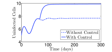
Figure 1. The evolution of the uninfected cells during time.

Figure 2 shows that, with control, the number of infected cells are significantly reduced after few weeks of therapy. Nevertheless, without control, this number remains much higher.

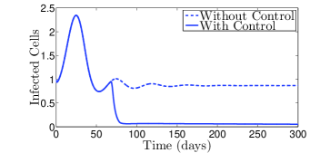
Figure 2. The evolution of the infected cells during time.

Figure 3 shows that, with control, the viral load decreases towards a very low level after the first days of therapy, whereas, without control, it remains much higher. This indicates the impact of the administrated therapy in controlling viral replication.

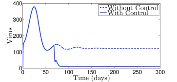
Figure 3. The evolution of the HIV virus during time.

Figures 4 and 5 show the adaptive immune response as function of time. The adaptive immunity is clearly affected by the control. Their curves converge towards zero with control, whereas, without any control, it converges towards $66.2721$ for CTL cells and converge towards $48.888$ for antibodies immune response.

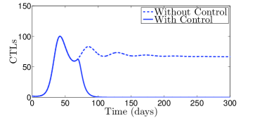
Figure 4. The evolution of the CTL cells during time.

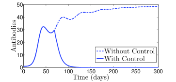
Figure 5. The evolution of the antibodies during time.

We note that all the curves (without control) of previous figures converge towards the endemic point with coordinates $(7.6923,0.8666,120,66.2721,48.888)$. This result is in good agreement with the result of Proposition 6, since with our chosen parameters we have $R_{0}=2.0833>1$, $R^{CTL,W}_{1}=1.2037>1$, and $R^{CTL,W}_{2}=1.3313>1$. The behavior of the two treatments during time is given in Fig. 6. The curves present the drug administration schedule during the time of treatment. This figure shows that we should give more importance to the first drug (RTIs) than to the second one (PIs).

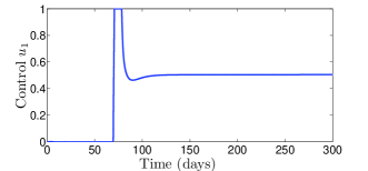
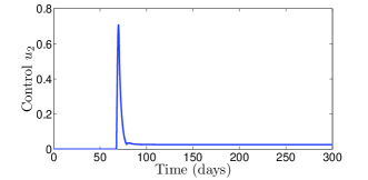
Figure 6. The behaviour of the two optimal controls.

6. Conclusion

In this work, we proposed and studied a mathematical model describing the human immunodeficiency virus with adaptive immune response and a trilinear antibody growth function. The main novelty in the model is to consider that the antibody growth depends not only on the virus and on the antibodies concentration but also on the uninfected cells concentration, which is supported by recent medical discoveries. After proposing the new mathematical model, positivity and boundedness of solutions were established. Then, local stability of the disease free steady state and the infection steady states was investigated. Next, an optimal control problem was proposed and studied. Two types of treatments were incorporated into the model: the purpose of the first consists to block the viral proliferation, while the role of the second one is to prevent new infections. Finally, numerical simulations were performed, confirming the stability of the free and endemic equilibria and illustrating the effectiveness of the two incorporated treatments via optimal control.

Received 01-June-2019; revised 10-May-2021; accepted 21-May-2021.

References

- [1] (3813045) [10.1007/s11786-018-0333-9] K. Allali, S. Harroudi and D. F. M. Torres, Analysis and optimal control of an intracellular delayed HIV model with CTL immune response, Math. Comput. Sci. 12 (2018), no. 2, 111–127. \arXiv1801.10048
- [2] (3716907) [10.1051/mmnp/201712501] K. Allali, Y. Tabit and S. Harroudi, On HIV model with adaptive immune response, two saturated rates and therapy, Math. Model. Nat. Phenom. 12 (2017), no. 5, 1–14.
- [3] (2211925) [10.1016/j.mbs.2005.12.006] M. S. Ciupe, B. L. Bivort, D. M. Bortz and P. W. Nelson, Estimating kinetic parameters from HIV primary infection data through the eyes of three different mathematical models, Math. Biosci. 200 (2006), no. 1, 1–27.
- [4] (2067116) [10.1007/s00285-003-0245-3] R. Culshaw, S. Ruan and R. J. Spiteri, Optimal HIV treatment by maximising immune response, J. Math. Biol. 48 (2004), no. 5, 545–562.
- [5] [10.1128/JVI.78.18.10096-10103.2004] M. P. Davenport, R. M. Ribeiro and A. S. Perelson, Kinetics of virus-specific CD8+ T cells and the control of Human Immunodeficiency Virus infection, J. Vir. 78 (2004), no. 18, 10096–10103.
- [6] (3046079) [10.1016/j.jtbi.2012.12.025] R. J. De Boer and A. S. Perelson, Quantifying T lymphocyte turnover, J. Theoret. Biol. 327 (2013), 45–87.
- [7] (3804169) [10.1007/s40314-017-0438-9] R. Denysiuk, C. J. Silva and D. F. M. Torres, Multiobjective optimization to a TB-HIV/AIDS coinfection optimal control problem, Comput. Appl. Math. 37 (2018), no. 2, 2112–2128. \arXiv1703.05458
- [8] (3808514) [10.1016/j.aml.2018.05.005] J. Djordjevic, C. J. Silva and D. F. M. Torres, A stochastic SICA epidemic model for HIV transmission, Appl. Math. Lett. 84 (2018), 168–175. \arXiv1805.01425
- [9] (0454768) W. H. Fleming and R. W. Rishel, Deterministic and stochastic optimal control, Springer-Verlag, Berlin, 1975.
- [10] (669666) I. S. Gradshteĭn and I. M. Ryzhik, Table of integrals, series, and products, Math. Comp. 39 (1982), no. 160, 747–757.
- [11] [10.3934/Math.2019.1.86] O. Kostylenko, H. S. Rodrigues and D. F. M. Torres, The spread of a financial virus through Europe and beyond, AIMS Mathematics 4 (2019), no. 1, 86–98. \arXiv1901.07241
- [12] (668522) D. L. Lukes, Differential equations, Mathematics in Science and Engineering, 162, Academic Press, Inc., London, 1982.
- [13] (3831969) [10.3934/jdg.2018016] C. C. McCluskey and M. Santoprete, A bare-bones mathematical model of radicalization, J. Dyn. Games 5 (2018), no. 3, 243–264.
- [14] [10.1016/0025-5564(91)90037-J] M. A. Nowak and R. M. May, Mathematical biology of HIV infections: antigenic variation and diversity threshold, Math. Biosci. 106 (1991), no. 1, 1–21.
- [15] (2009143) M. A. Nowak and R. M. May, Virus dynamics, Oxford University Press, Oxford, 2000.
- [16] (2901030) [10.1016/j.mbs.2011.11.002] K. A. Pawelek, S. Liu, F. Pahlevani and L. Rong, A model of HIV-1 infection with two time delays: mathematical analysis and comparison with patient data, Math. Biosci. 235 (2012), no. 1, 98–109.
- [17] (1669741) [10.1137/S0036144598335107] A. S. Perelson and P. W. Nelson, Mathematical analysis of HIV-1 dynamics in vivo, SIAM Rev. 41 (1999), no. 1, 3–44.
- [18] [10.1126/science.271.5255.1582] A. S. Perelson, A. U. Neumann, M. Markowitz, J. M. Leonard and D. D. Ho, HIV-1 dynamics in vivo: virion clearance rate, infected cell life-span, and viral generation time, Science 271 (1996), no. 5255, 1582–1586.
- [19] (0166037) L. S. Pontryagin, V. G. Boltyanskii, R. V. Gamkrelidze and E. F. Mishchenko, The mathematical theory of optimal processes, Interscience Publishers John Wiley & Sons, Inc. New York, 1962.
- [20] (3783261) [10.1002/mma.4207] D. Rocha, C. J. Silva and D. F. M. Torres, Stability and optimal control of a delayed HIV model, Math. Methods Appl. Sci. 41 (2018), no. 6, 2251–2260. \arXiv1609.07654
- [21] (3721854) [10.3934/dcdsb.2018030] F. Rodrigues, C. J. Silva, D. F. M. Torres and H. Maurer, Optimal control of a delayed HIV model, Discrete Contin. Dyn. Syst. Ser. B 23 (2018), no. 1, 443–458. \arXiv1708.06451
- [22] (3872461) [10.1016/j.physa.2018.10.033] S. Saha and G. P. Samanta, Modelling and optimal control of HIV/AIDS prevention through PrEP and limited treatment, Phys. A 516 (2019), 280–307.
- [23] [10.1155/2014/248407] C. J. Silva and D. F. M. Torres, Modeling TB-HIV syndemic and treatment, J. Appl. Math. 2014 (2014), Art. ID 248407, 14 pp. \arXiv1406.0877
- [24] (3392642) [10.3934/dcds.2015.35.4639] C. J. Silva and D. F. M. Torres, A TB-HIV/AIDS coinfection model and optimal control treatment, Discrete Contin. Dyn. Syst. 35 (2015), no. 9, 4639–4663. \arXiv1501.03322
- [25] [10.1016/j.ecocom.2016.12.001] C. J. Silva and D. F. M. Torres, A SICA compartmental model in epidemiology with application to HIV/AIDS in Cape Verde, Ecological Complexity 30 (2017), 70–75. \arXiv1612.00732
- [26] (3703337) [10.1501/Commua1_0000000833] C. J. Silva and D. F. M. Torres, Global stability for a HIV/AIDS model, Commun. Fac. Sci. Univ. Ank. Sér. A1 Math. Stat. 67 (2018), no. 1, 93–101. \arXiv1704.05806
- [27] (3714435) [10.3934/dcdss.2018008] C. J. Silva and D. F. M. Torres, Modeling and optimal control of HIV/AIDS prevention through PrEP, Discrete Contin. Dyn. Syst. Ser. S 11 (2018), no. 1, 119–141. \arXiv1703.06446
- [28] [10.1016/j.idm.2017.06.002] P. van den Driessche, Reproduction numbers of infectious disease models, Infect. Dis. Model. 2 (2017), no. 3, 288–303.
- [29] (3096543) [10.1007/s00285-012-0580-3] Y. Wang, Y. Zhou, F. Brauer and J. M. Heffernan, Viral dynamics model with CTL immune response incorporating antiretroviral therapy, J. Math. Biol. 67 (2013), no. 4, 901–934.
- [30] (2273003) [10.1007/978-0-387-68733-9] D. Wodarz, Killer cell dynamics, Interdisciplinary Applied Mathematics, 32, Springer-Verlag, New York, 2007.
- [31] (2525152) [10.3934/dcdsb.2009.12.511] H. Zhu and X. Zou, Dynamics of a HIV-1 infection model with cell-mediated immune response and intracellular delay, Discrete Contin. Dyn. Syst. Ser. B 12 (2009), no. 2, 511–524.