Viscous flows in hyperelastic chambers

Abstract

Viscous flows in hyperelastic chambers are relevant to many biological phenomena such as inhalation into the lung’s acinar region and medical applications such as the inflation of a small chamber in minimally invasive procedures. In this work, we analytically study the viscous flow and elastic deformation created due to inflation of such spherical chambers from one or two inlets. Our investigation considers the shell’s constitutive hyperelastic law coupled with the flow dynamics inside the chamber. For the case of a narrow tube filling a larger chamber, the pressure within the chamber involves a large spatially uniform part, and a small order correction. We derive a closed-form expression for the inflation dynamics, accounting for the effect of elastic bi-stability. Interestingly, the obtained pressure distribution shows that the maximal pressure on the chamber’s surface is greater than the pressure at the entrance to the chamber. The calculated series solution of the velocity and pressure fields during inflation is verified by using a fully coupled finite element scheme, resulting in excellent agreement. Our results allow estimating the chamber’s viscous resistance at different pressures, thus enabling us to model the process of inflation and deflation.

1 Introduction

The inflation of elastic balloons has been extensively investigated in the past, mainly because the corresponding dynamics depend on both the flow and the balloon’s material elasticity model. The inflation of a toy balloon or a spherical membrane was studied thoroughly by Beatty. In his work, Beatty has presented an analysis of an incompressible, isotropic hyperelastic spherical pressurized membrane. According to his work, and similar results by Treloar, the Mooney-Rivlin elasticity model successfully captures most of the overall physical effect. The majority of the research done so far considered hydrostatic uniform pressure distribution within the chamber and the determination of pressure as a constant parameter that uniformly affects the elastic walls (Needleman; Treloar; Beatty; Vandermarliere; Hines; Mangan).

Balloons with controlled inflation are used in medical applications such as pleural pressure assessments (Milic-Emili), and enteroscopy (Yamamoto). A recent study by Manfredi shows a promising biomedical application of a soft robot for a colonoscopy, which utilizes a double-balloon system for achieving inchworm-like crawling while bracing against the colonic walls. Haber investigated alternating shear flow over a self-similar, rhythmically expanding hemispherical depression. Quasi-steady creeping flow in models of small airway units of the lung was investigated by Davidson. Ilssar studied the inflation and deflation dynamics of a liquid-filled hyperelastic balloon, focusing on inviscid laminar flow. In those systems, the characteristic time it takes for the pressure to reach a constant uniform value in a chamber is assumed to be much shorter than the time it takes for the fluid to pass through the tubes (based on the viscous resistance). However, to assess the fluid and elastic shell’s dynamics, a complete mathematical model describing the system’s fluid-structure interaction at Low-Reynolds numbers is needed. The study of the fluid-structure interaction dynamics of low-Reynolds-number incompressible liquid flows and elastic structures may help introduce a new level of control in fluid-structure based autonomous systems due to the presence of viscous force (Elbaz14; Elbaz16).

In the Soft-Robotics field, recent studies show the propulsion of elastic structures embedded with internal cavities while controlling pressures or flow rates at the network’s inlets (BenHaim; Salem; Gamus; Siefert; Fei14; Fei16; Overvelde; Gorissen). In the case of fluidic actuation, several works study variations of the well-known ‘two-balloon system’, whereas others study networks of multiple connected chambers (BenHaim; Dreyer; Treloar; Glozman). As shown by these studies, for some given values of the pressure, multiple solutions for the volume are possible. Since the hyperelastic spherical membranes are multi-stable systems, it allows us to selectively inflate each balloon to one of its stable states by varying the input according to a particular carefully synthesized profile. Consequently, it can pave the way toward manufacturing soft robots that utilize minimal actuation to produce highly complex locomotion.

In this work, we examine the effect of elasticity on transient creeping flow in the bi-stable hyperelastic chambers. The chamber is assumed to be an ideal sphere. Stokes equation governs the flow field, while Mooney-Rivlin constitutive laws model the elastic chamber. The fluidic pressure within the balloon is not uniform and cannot be directly determined from the known Mooney-Rivlin relation. The fluidic pressure distribution in the chamber is estimated by balancing the fluidic pressure with the total force on the elastic membrane. Since this force is obtained by integrating the pressure distribution (which depends on the angle $\theta$), it receives a different value than the value obtained in the hydrostatic models.

This work’s structure is as follows: in § 2, the geometry, relevant parameters and physical assumptions are defined. In § 3, the hyperelastic Mooney-Rivlin constitutive law is presented. The strain energy function is analyzed in order to present the bi-stable phenomena. Section § 4 presents closed-form solutions of the governing equations, describing the flow field within an expanding chamber. In § LABEL:sec:Results, two different physical cases are described. The case of dictated inlet mass rate coupled by the hyperelastic model is described in § LABEL:Dynamic_case_II, where numerical verification of the fully coupled model is presented. In § LABEL:Dynamic_case_III, we present the second case where the inlet pressure is dictated and the stretching of the hyperelastic sphere is governed by the flow dynamics. Section § LABEL:TwoBalloons examines the dynamic behavior of two interconnected bi-stable chambers. Concluding remarks are presented in § LABEL:Concludings.

2 Problem Formulation

In this section, we present the problem definition, along with the physical parameters relevant to the analysis and the small non-dimensional parameters. The examined liquid-filled chamber is illustrated in Figure 1. Here, a spherical geometry is assumed (the validity of this assumption will be verified by numerical simulation in §LABEL:Dynamic_case_II). A spherical hyperelastic chamber with a stress-free radius of $r_{0}$, is connected to two rigid tubes with radius $a$ and length $\ell$. For simplicity, we assume identical tubes in the inlet and the outlet. Here, the flow-field inside the chamber and tubes is considered incompressible, Newtonian, and with negligible inertial effects. The fluid’s axial velocity inside the tube is $u_{z}$, and the volumetric flux rate is denoted $q(t)$ (where $q_{in}(t)$ refers to the flow entering the body from the inlet tube and $q_{out}(t)$ refers to the flow moving from the body through the outlet tube). The relevant variables and parameters are the time $t$, the axial coordinate and symmetry axis $z$, and the radial coordinate $s$ of the cylindrical system used to describe the tubes. Axisymmetry allows us to eliminate the azimuthal angle of the cylindrical system. Furthermore, the pressure and flow velocity fields of the entrapped fluid are $p(t,s,z)$ and $\textbf{v}(t,s,z)$, while its constant density and dynamic viscosity are denoted $\rho$ and $\mu$. The chamber’s dynamics are approximated by a single degree of freedom, represented here by the chamber’s instantaneous radius, denoted $\eta(t)$. For spherical geometry, a coordinate system is chosen so that one of the coordinates remains constant on the boundary. Here, $\{r,\theta,\phi\}$ are the coordinates of a moving spherical system, located at the center of the chamber, where $\theta$ is the polar angle, measured from the axis of symmetry to the radial coordinate $r$, and $\phi$ is the azimuthal angle, revolving around the axis of symmetry, $z$. The Cauchy-stress tensor of the flow is denoted as $\mathbf{\sigma}_{\mathbf{f}}$. The stress-free shell’s thickness is $w_{0}$, which is considered to be much smaller than the stress-free chamber’s radius, namely $w_{0}\ll r_{0}$.

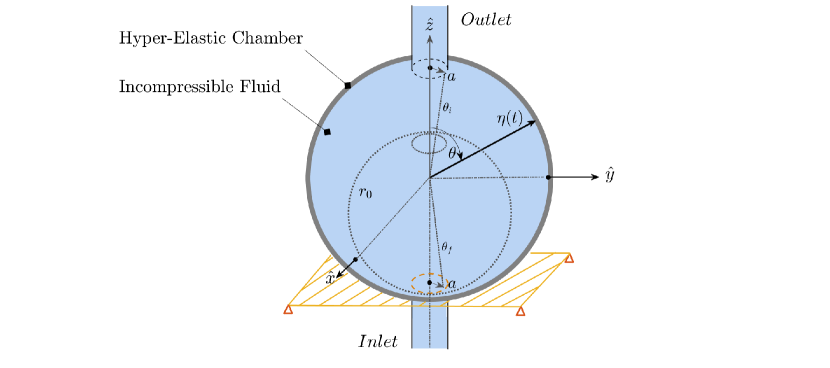
Figure 1: Illustration of the system under investigation, consisting of a hyper-elastic chamber, as well as a fixed inlet tube, and a massless outlet tube, both having identical radius and length. The bottom of the chamber is held fixed during the inflation, while its center is allowed to move.

The following analysis utilizes three small parameters, including the ratio between the radius of the tubes and the radius of the stress-free chamber ($\varepsilon_{a}$, denoted hereafter by tube-chamber radii ratio),

$$\epsilon_{a}=\cfrac{a}{r_{0}}\ll 1,$$ (1)

the slenderness of the tubes ($\varepsilon_{t}$, denoted hereafter by tube slenderness),

$$\epsilon_{t}=\cfrac{a}{\ell}\ll 1,$$ (2)

and the last small parameter in the analysis is taken as the ratio between the viscous stresses and the overall pressure in the chamber ($\varepsilon$, denoted hereafter by chamber viscous resistance parameter), defined by

$$\varepsilon=\cfrac{\mu v^{*}}{r_{0}p^{*}}\ll 1,$$ (3)

where $v^{*}$ is the characteristic flow velocity in the chamber, and $p^{*}$ is the characteristic pressure of the system. For the following analysis, we shall normalize the physical variables by considering the characteristic values of the problem as follows:

$$\textbf{V}=\cfrac{\boldsymbol{v}}{v^{*}},\quad\hat{\boldsymbol{\nabla}}=r_{0}\boldsymbol{\nabla},\quad\hat{\boldsymbol{\sigma_{f}}}=\cfrac{\boldsymbol{\sigma_{f}}}{p^{*}},\quad R=\cfrac{r}{r_{0}},\quad\lambda=\frac{\eta}{r_{0}},\quad P=\cfrac{p}{p^{*}},\quad T=\cfrac{t}{r_{0}/v^{*}},$$ (4)

where $\lambda(T)$ denotes the stretch of the chamber, and $R$ is the normalized radial coordinate.

3 Constitutive model for a hyperelastic membrane

This section presents the constitutive law that governs the spherical shell dynamics. We consider a thin-shelled, spherical chamber made of incompressible hyperelastic isotropic material. Finite elasticity theory dictates a known form of the elastic strain energy density $\psi(\lambda)$, which depends only on the relative stretch $\lambda(T)$. Moreover, the elastic strain energy density satisfies $\psi(1)=0$. Different types of hyperelastic models differ in the type of material and the elastic strains experienced without failing. The most common models are neo-Hookean, Mooney-Rivlin, Ogden, Gent and Biological tissue (Ogden).

The material is assumed to be incompressible, which leads to the relation between the pressurized and the stress-free states, given by $r^{2}w\approx r_{0}^{2}w_{0}$. Thanks to this relation, the chamber’s instantaneous thickness is eliminated. To capture the chamber’s bi-stability, we use the two-parameter Mooney-Rivlin model.

Under the above assumptions, and considering incompressibility, the normalized solid’s Mooney-Rivlin strain energy function is given by (Ogden; Beatty),

$$\hat{\psi}(\lambda)=2\lambda^{2}+\cfrac{1}{\lambda^{4}}-3+\alpha\bigg{(}\lambda^{4}+\cfrac{2}{\lambda^{2}}-3\bigg{)}$$ (5)

where $\alpha=s_{2}/s_{1}$ is the ratio between two empirically determined constants, commonly denoted as the Mooney–Rivlin parameters.

In this study, the Mooney–Rivlin parameters are chosen as $s_{1}\approx 1.5$ MPa and $s_{2}\approx 0.15$ MPa (Beatty; Treloar). The normalized equation (5) was obtained by using the normalization $\psi^{*}=s_{1}$ for the strain energy density function, and the magnitude of the parameter $\alpha$ is $O(10^{-1})$.

We first study the chamber’s static behavior, where the pressure (without flow) is dictated. In this case, both the stretch and the pressure are constant, denoted here by $\lambda_{SS}$ and $P_{SS}$, respectively. The behavior mentioned above can be demonstrated by the overall effective potential energy of the system,

$$\mathcal{U}(\lambda_{SS};P_{SS})=\int_{\lambda_{SS}}{\bigg{(}\cfrac{d\hat{\psi}}{d\xi}-\xi^{2}P_{SS}}\bigg{)}\mathrm{d}\xi=\hat{\psi}(\lambda_{SS})-\frac{1}{3}\lambda_{SS}^{3}P_{SS}.$$ (6)

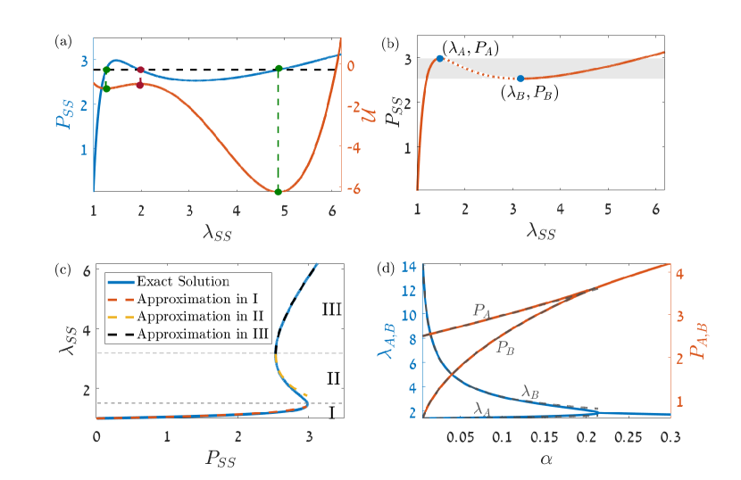
Figure 2: (a) - The solid blue curve is a characteristic stretch–pressure curve of a single elastic chamber with $\alpha=0.1$. The solid orange curve is the effective potential energy function (6), corresponding to the constant pressure $P_{SS}=2.75$, illustrated by the dashed black line; Green and red dots are the stable and unstable equilibrium radii. (b) - Characteristic normalized stretch–pressure curve of a single elastic chamber according to (7) with $\alpha=0.1$. The extrema are marked, and the bi-stable region is marked in grey. Solid curves are stable branches and dashed curves are unstable ones. (c) - The solid blue line is the exact solution of (7) calculated numerically. The dashed curves are the approximated solutions obtained in (LABEL:delta1Appr)-(LABEL:delta2Appr). (d) - The evolution of the extremum values of pressure $P_{A},P_{B}$ and stretch $\lambda_{A},\lambda_{B}$ as a function of the small parameter $\alpha$. The solid curves are the exact values, and the dashed curves are the asymptotic approximations given in appendix (LABEL:PAapprox),(LABEL:PBappr).

Based on (6), Figure 2(a) shows a curve of the potential energy function where the constant pressure is $P_{SS}=2.75$. The Mooney-Rivlin relation (5), along with the steady version of the leading order energy balance (6), formulated as $\partial\mathcal{U}/\partial\lambda_{SS}=0$ at constant pressure $P_{SS}$, yields a relation between stretch, $\lambda_{SS}$, and pressure, $P_{SS},$ in equilibrium condition,

$$P_{SS}=\bigg{(}\cfrac{1}{\lambda^{2}}\frac{d\hat{\psi}}{d\lambda}\bigg{)}\bigg{|}_{\lambda_{SS}}=4\bigg{[}\frac{1}{\lambda_{SS}}-\frac{1}{\lambda^{7}_{SS}}+\alpha\bigg{(}\lambda_{SS}-\frac{1}{\lambda^{5}_{SS}}\bigg{)}\bigg{]};\qquad 0<\alpha\ll 1.$$ (7)

This well-known relation was extensively leveraged to describe the quasi-static inflation of spherical balloons (Beatty; Treloar; BenHaim) for spatially uniform pressures. As seen from Figure 2(a), showing the relation in (7) with $\alpha=0.1$, the uniform pressure of the chamber is not monotonic with respect to the radius. Therefore, the inverse relation, describing the chamber’s radius as a function of the pressure, cannot be directly extracted. The curve $P_{SS}(\lambda_{SS})$ in Figure 2(b) has two bifurcation points, described by a local maximum point at $(\lambda_{A},P_{A})$, and a local minimum point at $(\lambda_{B},P_{B})$. This figure shows a bifurcation, which occurs when the pressure enters or exits the range between the local extrema, $P_{B}<P_{SS}<P_{A}$, illustrated in grey. Asymptotic approximations for the bifurcation points of the equilibrium curve, $P_{A},P_{B},\lambda_{A}$ and $\lambda_{B}$, appears in Appendix LABEL:appA. The evolution of those extrema as a function of the small parameter $\alpha$ is presented in Figure 2(d). Asymptotic approximations for the solution of the equilibrium equation (7), appear in Appendix LABEL:appA. Those approximations are plotted in Figure 2(c) with dash-lines on the solid exact solution curves, represented by the inverse relation $\lambda_{SS}(P_{SS})$.

Analyzing the strain energy function $\mathcal{U}(\lambda_{SS};P_{ss})$ in Equation (6), using the second derivative with respect to $\lambda_{SS}$, it can be proven that the right and left branches of $P_{SS}(\lambda_{SS})$ where $1<\lambda<\lambda_{A}$ or $\lambda_{B}<\lambda$ are stable equilibria and satisfy,

$$\cfrac{\partial^{2}\mathcal{U}}{\partial\lambda_{SS}^{2}}\bigg{|}_{P_{SS}}=\cfrac{dP_{SS}}{d\lambda_{SS}}>0.$$ (8)

Conversely, the intermediate branch $\lambda_{A}<\lambda_{SS}<\lambda_{B}$ is an unstable region satisfying $\partial^{2}\mathcal{U}/\partial\lambda_{SS}^{2}<0$. This is precisely the bi-stability phenomenon.

4 Series solution of the flow-field within an expanding chamber

In this section, the governing equations of the flow within the chamber will be formulated, as well the problem’s boundary conditions. An analytical series solution will then be presented, describing the velocity field and the flow’s pressure distribution inside the spherical chamber.

4.1 Formulation and analysis of the governing equations

Under the assumptions discussed above, the momentum and continuity equations governing the fluid’s behavior expressed in the moving spherical frame: ρ(∂v∂t+vv+^zd2dt2η^2-a^2)& = -p+μ^2v-ρg^z ,
v = 0 , where the third term in the left expression in the momentum equation (4.1a) describes the acceleration of the moving spherical frame, centered on the chamber’s moving center, relative to a stationary frame.

Assuming the flow in tubes is fully developed and axisymmetric, the volumetric flux is given by,

$$q(t)=-\cfrac{\pi a^{4}}{8\mu}\frac{\partial p_{t}}{\partial{z}},$$ (9)

where $\partial p_{t}/\partial z$ is the pressure gradient along the tube. Since the tube slenderness $\epsilon_{t}\ll 1$ we shall assume a constant pressure gradient. Normalization of (9) yields the characteristic flow rate as $q^{*}=\pi a^{2}u_{z}^{*}$ where $u_{z}^{*}=a^{2}p^{*}/\mu\ell$ is the characteristic axial component of the fluid velocity in the tube. An integral flow balance yields the relation between the characteristic velocity in the tube and the characteristic velocity of the flow within the chamber, as $v^{*}=\epsilon_{a}^{2}u_{z}^{*}$. Substituting the characteristic values into the chamber viscous resistance parameter (3), relates it to the other small parameters, as follows

$$\varepsilon=\frac{a^{4}}{r_{0}^{3}\ell}=\epsilon^{3}_{a}\epsilon_{t}\ll 1.$$ (10)

From relation (10) it is clear that $\varepsilon$ is dependent merely on the geometry of the system, providing a simple relation between the hydrostatic and deviatoric stresses. Hence, an appropriate geometry can be defined in order to design an efficient and controllable system. We consider negligible gravity, i.e., $\rho gr_{0}/p^{*}\ll 1$ (where $g$ is the gravitational acceleration), and define a Reynolds number in chamber as $\Rey=\rho v^{*}r_{0}/\mu\ll 1$. Since the Reynolds number is small, the flow’s inertia may be neglected. Therefore, by utilizing the non-dimensional quantities specified in (4) the fluid’s motion (4.1) is governed by Stokes equations for creeping flow with an implicit time variable,

$$\hat{\bnabla}\bcdot\boldsymbol{V}=0,\quad\hat{\bnabla}P=\varepsilon\hat{\bnabla}^{2}\boldsymbol{V}+O(\varepsilon\Rey).$$ (11)

The validity of these equations is weakened at the vicinity of the connections to the tubes since in those regions, the characteristic velocity is approximately $u_{z}^{*}$ rather than $v^{*}$. At a distance $O(L)$ from the tube (where $a<L<r_{0}$), the velocity scale is $q^{*}/L^{2}$ and hence the Reynolds number is $\rho q^{*}/\mu L<\rho q^{*}/\mu a$. Thus, a sufficient condition for global neglect of inertia is,

$$q^{*}\ll\cfrac{\pi\mu a}{\rho}.$$ (12)

From the non-dimensional relation (11), in the sphere, the pressure is spatially uniform at leading order and the viscous flow will generate small spatially varying corrections. Moreover, in order to get a better understanding of the chamber resistance small parameters’ physical meaning, we may use the dynamical stress tensor in the fluid domain defined by the constitutive relation $\boldsymbol{\sigma_{f}}=-p\boldsymbol{I}+\mu\big{[}\boldsymbol{\nabla v}+(\boldsymbol{\nabla v})^{T}\big{]}$ where $\boldsymbol{I}$ is the $3\times 3$ unit matrix. In the most general constitutive equation, $\boldsymbol{\sigma}_{f}$ consisting of the linear and instantaneous dependence of the deviatoric stress, plus the hydrostatic stress, $-p\boldsymbol{I}$, stemming from the static pressure. Normalization of the total stress tensor yields,

$$\boldsymbol{\hat{\sigma}_{f}}=-P\boldsymbol{I}+\varepsilon\big{[}\boldsymbol{\hat{\nabla}V}+\big{(}\boldsymbol{\hat{\nabla}V}\big{)}^{T}\big{]}.$$ (13)

As one can notice from equation (13) the velocity field is not included at the leading-order. Mainly, the leading-order of the problem is a case of fully developed uniform pressure without any velocities. Suppose the flow is dictated by controlled pressure or flux at the inlet, the velocity is generated, and additional small deviatoric stress is created, which quasi-statically leads the system to another hydrostatic state.

The axisymmetric Stokes equations (11) can be solved in spherical polar coordinates using a series expansion (Happel). Consider the non-dimensional Stokes stream function $\Psi(R,\theta,T)$. The flow velocity components $V_{R}$ and $V_{\theta}$ are related to the Stokes stream function $\Psi(R,\theta,T)$ through

$$V_{R}=\cfrac{1}{R^{2}\sin\theta}\cfrac{\partial\Psi}{\partial\theta};\quad V_{\theta}=-\cfrac{1}{R\sin\theta}\cfrac{\partial\Psi}{\partial R},$$ (14)

where $V_{R}$ and $V_{\theta}$ are the radial and tangential velocity components, respectively. By applying the curl operator to the momentum equation (11) and using several simple algebraic manipulations, the Stokes equation can be reduced to a fourth-order bi-harmonic equation obtained in terms of the Stokes stream function as follows: E^2(E^2Ψ) = 0 ,    
P = -ε