Sharp exponent of acceleration in general nonlocal equations with a weak Allee effect

Abstract

We study an acceleration phenomenon arising in monostable integro-differential equations with a weak Allee effect. Previous works have shown its occurrence and have given correct upper bounds on the rate of expansion in some particular cases, but precise lower bounds were still missing. In this paper, we provide a sharp lower bound for this acceleration rate, valid for a large class of dispersion operators. Our results manage to cover fractional Laplace operators and standard convolutions in a unified way, which is new in the literature. A first very important result of the paper is a general flattening estimate of independent interest: this phenomenon appears regularly in acceleration situations, but getting quantitative estimates is most of the time open. This estimate at hand, we construct a very subtle sub-solution that captures the expected dynamics of the accelerating solution (rates of expansion and flattening) and identifies several various regimes that appear in the dynamics depending on the parameters of the problem.

Keywords: generic nonlocal dispersion operators, fractional laplacian, convolution operator, acceleration, level lines.

1 Introduction

In this paper, we are interested in describing quantitatively the propagation phenomenon in the following (non-local) integro-differential equation, complemented with an initial condition:

$$u_{t}(t,x)={\mathcal{D}}[\,{u}\,](t,x)+f(u(t,x))\quad\text{ for }\quad t>0,\ x\in\mathbb{R},$$ (1.1)

$$u(0,x)=u_{0}(x)\quad\text{ for }\quad x\in\mathbb{R},$$ (1.2)

where the function $u$ represents a density of population and thus takes its values in $[0,1]$, the function $f$ is a monostable nonlinearity to be specified, the nonnegative function $u_{0}$ is the initial density, and the dispersal operator ${\mathcal{D}}[\,{\cdot}\,]$ is defined by

$${\mathcal{D}}[\,{u}\,](t,x):=\mathrm{P.V.}\left(\int_{\mathbb{R}}[u(t,y)-u(t,x)]J(x-y)\,dy\right),$$

the kernel $J$ being a nonnegative function satisfying the following properties.

Hypothesis 1.1.

Let $s$ be a positive real number. The kernel $J$ is nonnegative, symmetric and such that there exist positive constants ${\mathcal{J}}_{0}$, ${\mathcal{J}}_{1}$ and $R_{0}\geq 1$ verifying

$$\int_{-1}^{1}J(z)z^{2}\,dz\leq 2{\mathcal{J}}_{1}\quad\text{ and }\quad\frac{{\mathcal{J}}_{0}}{|z|^{1+2s}}\mathds{1}_{\{|z|\geq 1\}}(z)\geq J(z)\geq\frac{{{\mathcal{J}}_{0}}^{-1}}{|z|^{1+2s}}\mathds{1}_{\{|z|\geq R_{0}\}}(z).$$

The operator ${\mathcal{D}}[\,{\cdot}\,]$ describes the dispersion process of individuals. Roughly speaking, the value of $J(x-y)$ gives the probability of a jump from position $x$ to position $y$, which makes the tails of the dispersal kernel $J$ of crucial importance when quantifying the dynamics of the population. As a matter of fact, the parameter $s$ will appear in the rates we obtain. One may readily notice that the hypothesis on $J$ allows us to cover the two main types of integro-differential operators usually considered in the literature: the fractional Laplace operator $(-\Delta)^{s}u$ on the one hand, and a standard convolution operator with an integrable kernel, often written $J\star u-u$, on the other. This universality is one of the main contributions of the present paper.

Without further notice, we will assume that $f$ satisfies the following.

Hypothesis 1.2.

The nonlinearity $f$ belongs to $\mathscr{C}^{1}([0,1],\mathbb{R})$ and is of the monostable type, in the sense that

$$\begin{cases}f(0)=f(1)=0,\quad f(u)>0\quad\text{for}\quad u\in(0,1),\vskip 6.0pt plus 2.0pt minus 2.0pt\\ f^{\prime}(1)<0,\vskip 6.0pt plus 2.0pt minus 2.0pt\\ \displaystyle{\lim_{u\to 0}\frac{f(u)}{u^{\beta}}\geq r},\end{cases}$$

for some real numbers $r>0$ and $\beta>1$.

The parameter $\beta$ above describes the possibility of a weak Allee effect that the population has to overcome. A biological description and discussion about the origin and relevance of such an effect may be found in a book by Courchamp et al. [20], and also in [7, 27, 10]. In crude terms, the Allee effect means that a population with too few individuals will not be fit enough to persist and grow. It is is said to be weak whenever the growth rate of a very small population is eventually extremely small but still positive, as opposed to a strong effect, which leads to negative growth rates for small populations. In the sequel, and without further notice, we take $\beta>1$, thus yielding small growth rates for small densities, and assume that the initial datum satisfies the following hypothesis.

Hypothesis 1.3.

The initial datum $u_{0}$ belongs to $\mathscr{C}(\mathbb{R},[0,1])$ and is such that $1\geq u_{0}\geq a\mathds{1}_{(-\infty,b]}$ for some real numbers $a>0$ and $b$.

Existing works and previous results

Let us review the existing literature in order to position our work. Propagation phenomena in reaction-diffusion and integro-differential equations have been the object of intense studies in the last decades. Starting from the work of Fisher on the propagation of an advantageous gene [29] and its analysis by Kolmogorov, Petrovski and Piskunov [38] and related works by e.g. Aronson and Weinberger [8], the quantitative description of spreading gave birth to various mathematical tools and techniques such as travelling waves, accelerating profiles, transition fronts, among many others.

When $\beta=1$ and the nonlinearity $f$ satisfies $f(s)\leq f^{\prime}(0)s$, meaning it is a Fisher-KPP nonlinearity, it is known that solutions to problem (1.1)-(1.2) exhibit some propagation phenomenon: starting with a nonnegative nontrivial compactly supported initial datum, the corresponding solution $u$ converges to $1$ locally uniformly in space as time gets large. This is referred as the hair trigger effect [8]. Moreover, in many cases, this convergence can be precisely characterised. Indeed, when the dispersion kernel $J$ is exponentially bounded, travelling waves are known to exist and solutions to the Cauchy problem typically propagate at constant speed, see [46, 49, 19, 24, 23, 39, 50]. On the other hand, when the kernel $J$ possesses heavy tails, travelling waves do not exist and the solutions exhibit an acceleration phenomenon, see [40, 50, 30]. More precisely, Garnier [30] gave the first acceleration estimates and the first author with Garnier, Henderson and Patout [15] next provided sharp level sets for convolution operators; a group around Cabré and Roquejoffre [18, 17] studied the fractional Fisher-KPP equation concluding to an exponential propagation behaviour. A related, but different, acceleration phenomenon for positive solutions of a local Cauchy problem also appears in reaction-diffusion equations when playing with the tails of the initial datum [33]. We emphasise that, in the present work, the acceleration is solely due to the structure of the dispersal operator.

When an Allee effect is introduced, the study of propagation becomes more subtle. Alfaro [3] started a program with a paper about the interplay between a heavy tailed initial datum and the Allee effect in local reaction-diffusion equations. Coville et al. [24, 23, 22] have proved existence of travelling fronts when the dispersal kernel $J$ is exponentially bounded and the Cauchy problem typically does not lead to acceleration [51]. When not, the competition between heavy tails and the Allee effect leads to intense discussions. Gui and Huan [32] discussed the existence or not of travelling waves for a fractional equation with an Allee effect. They obtained existence (and thus propagation at a fixed speed) when $\tfrac{\beta}{2s(\beta-1)}<1$. However, neither a description of acceleration nor a precise rate of acceleration were given in the opposite case. In the same spirit, for algebraically decaying kernels, Alfaro and Coville [4] provided the exact separation between existence and non-existence of travelling waves for convolution type equations, showing the exact separation between non-accelerated and accelerated solutions in the Cauchy problem. Before reviewing the last-to-date results on problem (1.1)-(1.2), let us also mention that an acceleration phenomenon is also present in some porous medium equations, see [37, 47, 5, 6].

As far as problem (1.1)-(1.2) is concerned, bounds on the expansion of the level sets of solutions have been obtained by the second author with Gui and Zhao [25] and by Alfaro [4], showing a delicate interplay between the tails of $J$ and the parameter $\beta$. Namely, an upper bound for acceleration is known when ${\mathcal{D}}[\,{\cdot}\,]$ is a fractional Laplace operator (i.e., $J\propto|\cdot|^{-(1+2s)}$) or when the kernel $J$ is integrable with a finite first moment (which corresponds to having $s>\frac{1}{2}$): solutions spread as at most $t^{\frac{\beta}{2s(\beta-1)}}$ when $\tfrac{\beta}{2s(\beta-1)}>1$. However, these authors were unable to provide a matching lower bound, leaving the determination of the exact speed of the level lines an open question. We do not recall here the exact exponents they got in order to avoid misunderstandings while reading the present paper, but instead refer to [4] and [25] where they are given. Nevertheless, to provide a clear picture, we summarized in the Figures 1(a) and 1(b) the already known behaviours in these two particular situations.

(a) The convolution case

(b) The fractional case

Figure 1: For the convolution case, Figure 1(a), we have: In the green zone, the model enjoys linear propagation with existence of travelling fronts [21]: $x_{\lambda}(t)\asymp c^{*}t$. In the white zone ➌, no estimates are known. In the blue zone ➊, only an upper bound has been derived, see [4]: $x_{\lambda}(t)\lesssim t^{\frac{\beta}{2s(\beta-1)}}$. In the purple zone ➋, non matching lower and upper bounds have been derived [4]: $t^{\frac{1}{2s(\beta-1)}}\lesssim x_{\lambda}(t)\lesssim t^{\frac{\beta}{2s(\beta-1)}}$. The orange zone is a zone of exponential propagation, see Garnier [30], Bouin et al. [15]: $x_{\lambda}(t)\asymp\exp({\color[rgb]{0,0,1}\rho}t)$.
For the fractional case, Figure 1(b), we have: In the green zone, the model enjoys linear propagation with existence of travelling fronts [32, 25]: $x_{\lambda}(t)\asymp c^{*}t$. In the blue zone ➊, non matching upper and lower bounds have been derived, see [25]: $t^{\frac{1}{2s}}\lesssim x_{\lambda}(t)\lesssim t^{\frac{\beta}{2s(\beta-1)}}$. In the purple zone ➋, non matching lower and upper bounds have been derived, see [25]: $t^{\frac{1}{2s(\beta-1)}}\lesssim x_{\lambda}(t)\lesssim t^{\frac{\beta}{2s(\beta-1)}}$. The orange zone is a zone of exponential propagation, see Roquejoffre et al. [17]: $x_{\lambda}(t)\asymp\exp({\color[rgb]{0,0,1}\rho}t)$.

In a preliminary version of the present paper [14] (published during the completion of the current program) we provided, under the assumptions that $J$ satisfies Hypothesis 1.1 and that the parameter $s$ belongs to $(0,1)$, a lower bound for the acceleration of the level lines of solutions to (1.1)-(1.2), showing for the first time that the spreading is of order $t^{\frac{\beta}{2s(\beta-1)}}$ and thus getting a sharp exponent for acceleration. This preliminary result in hand, we were informed that Zhang and Zlatoš [52] had managed to obtain similar bounds in the particular case of a fractional Laplace operator, using a different approach that relies strongly on the properties of this fractional operator. The present version of our work introduces the full range of the general approach initiated in [14]. The sharp estimate is obtained with the fewest possible assumptions on the kernel $J$, in particular with the fewest restrictions on the parameter $s$.

Statement of the main result

To follow the propagation of the population modelled by system (1.1)-(1.2), we may define the level set of height $\lambda$, with $\lambda$ a real number in $(0,1)$, of a solution $u$ to the problem, that is

$$\forall t\in(0,+\infty),\ x_{\lambda}(t):=\sup\left\{x\in\mathbb{R},\,u(t,x)\geq\lambda\right\}.$$

Let us now state precisely our main result.

Theorem 1.4.

Assume that $J$, $u_{0}$ and $f$ respectively satisfy Hypotheses 1.1, 1.3 and 1.2 and that the parameters $s$ and $\beta$ are such that

$$\beta<1+\frac{1}{2s-1}.$$ (1.3)

Then, for any $\lambda$ in $(0,1)$, the level line $x_{\lambda}$ of a solution to problem (1.1)-(1.2) accelerates with a rate equal to $\frac{\beta}{2s(\beta-1)}$, that is

$$x_{\lambda}(t)\asymp_{\lambda}t^{\frac{\beta}{2s(\beta-1)}}.$$

To give the reader a clear panorama of the scope of this result, we have summarised previous contributions and ours in Figure 2.

Figure 2: In the green zone, based on the previous works [4, 21, 25, 32], the model is expected to enjoy a linear propagation with existence of travelling fronts: $x_{\lambda}(t)\sim c^{*}t$. In the blue zone, we provide the sharp lower and upper bounds : $x_{\lambda}(t)\asymp t^{\frac{\beta}{2s(\beta-1)}}$. The orange zone is a zone of exponential propagation, by straightforward extension of the work of Bouin et al. [15]: $x_{\lambda}(t)\asymp\exp(\rho t)$.

To the best of our knowledge, Theorem 1.4 provides the first sharp, unified, estimate for level sets in such a generic context. As we already mentionned, correct upper bounds in some particular settings had been previously derived, but no precise lower bound was provided in general. Note that condition (1.3) in Theorem 1.4 fits with and unifies the ones in the related papers [4, 14, 25, 32, 52]. Note that we also obtain the rate of invasion for a convolution operator when $s$ belongs to $(0,\frac{1}{2}]$, which remained open in [25].

The constructions made in [4, 25] to obtain upper bounds are robust and can be adapted to the range of parameters considered in the present paper for kernels satisfying Hypothesis 1.1. In order to avoid unnecessary computations, we will not duplicate them here. Our contribution is thus a generic way of obtaining a lower bound that matches the already known upper bounds.

Finally, let us illustrate our result with some numerical simulations (see Section 6 for details on the numerical approximation used). In Figure 3, the position of the level line of height $\lambda=0.5$ is plotted as a function of time for two different values of $\beta$ and several values of the fractional Laplacian exponent $s$. In one of the two configurations, namely for $\beta=1.5$, the theoretic critical value of the exponent $s$ above which there exists a travelling front is strictly greater than $1$. As a consequence, the level set accelerates for any of the chosen values for $s$ in $(0,1)$, but this acceleration clearly decreases to none as $s$ tends to $1$, as expected from the existing results for local diffusion.

This is no more the case for $\beta=3$, as one can observe a switching from an accelerated regime to a travel at constant speed around the critical value $s=0.75$ (the corresponding curve is plotted with a dashed line).

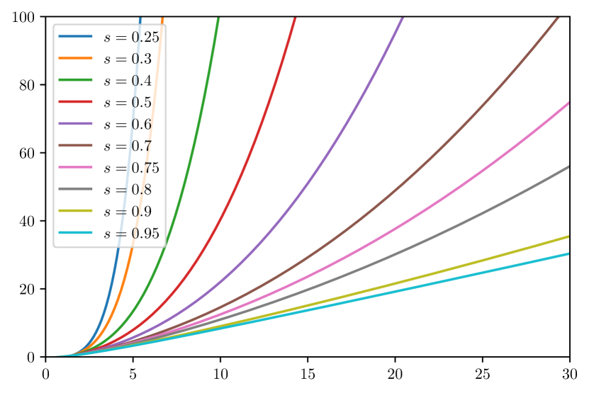
(a) $\beta=1.5$.

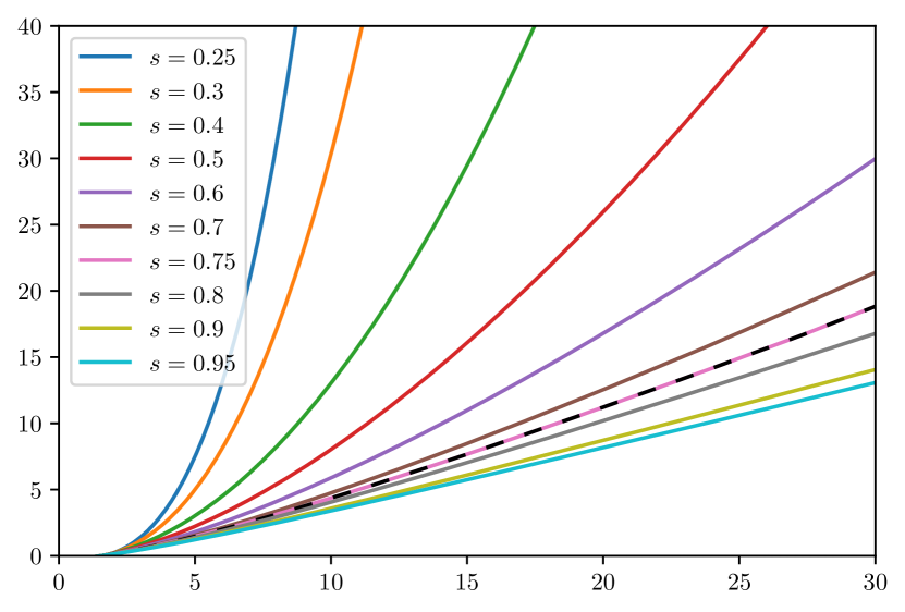
(b) $\beta=3$.

Figure 3: Position of the level line of height $\frac{1}{2}$ of numerical approximations of the solution to the problem with fractional diffusion, plotted as a function of time, for two different values of $\beta$ and several values of $s$ in $(0,1)$.

Comments on the strategy

The first step in proving the result is to study how the solution evolves from the initial datum for short times, and, in particular, what is decay at infinity created by the dispersion with fat tails. We prove in Proposition 2.2 that a solution to (1.1)-(1.2) with initial datum satisfying Hypothesis 1.3 behaves as $x^{-2s}$ at infinity at time $1$. When $s\geq 1$, this is enough to conclude.

When $s$ belongs to $(0,1)$, an important aspect is to know that a positive solution to (1.1)-(1.2), with $u_{0}$ satisfying Hypothesis 1.3, flattens through time, that is

$$\forall C>0,\quad\exists t_{C}>0,\quad\lim_{x\to+\infty}x^{2s}u(t,x)\geq C\quad\text{ for all }\quad t\geq t_{C}.$$

Figure 4 illustrates this particular behaviour using numerical simulations, showing the deformation of the profile of a solution over time. The flattening property is more clearly seen in the right hand side plot, where profiles of the solution at different times are shifted back to have the same value at $x=0$. We see that there is no stabilisation of the profile and that the shape of the solution keeps changing through time, which is usually not the case when the long time behaviour is a constant speed propagation.

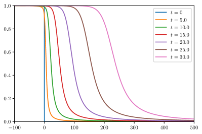
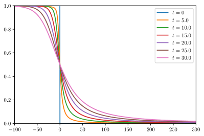
Figure 4: Numerical approximations of the solution to the problem with fractional diffusion at different times for $s$ equal to $0.6$ and $\beta$ equal to $1.5$. On the right, the graphs have been shifted by setting the position of the level line of value $\frac{1}{2}$ at $x=0$, for comparison purposes. The latter exhibits more clearly the deformation of the solution.

A more convincing picture of the flattening effect may be obtained by plotting the evolution over time of the best constant $C$ such that the tail of the solution fits with $\frac{C}{x^{2s}}$ in the least square sense. The graphs in Figure 5 show that, after a rapid transition, the constant grows linearly. We also refer to Figure 13 for various plots showing the adequation between $u(t,\cdot)$ and $x^{-2s}$ at the edge of the invasion profile.

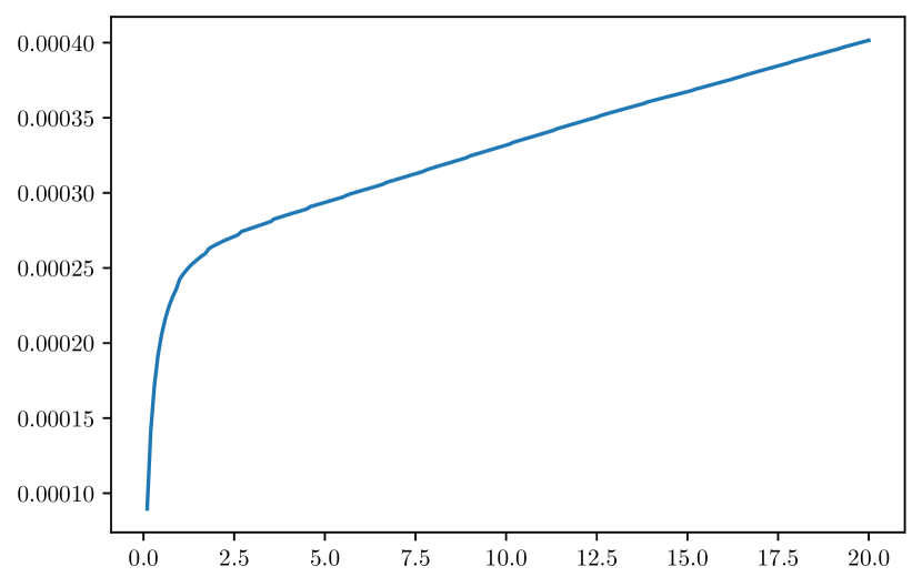
(a) $s=0.4$.

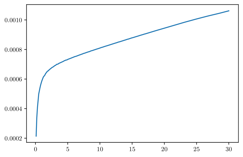
(b) $s=0.5$.

Figure 5: Evolution over time of the fitting constant for the part of the tail of the approximation solution at time $t=1$ bounded by value $10^{-2}$ on the left and value $10^{-5}$ on the right using the function $\frac{C}{x^{2s}}$ for the solution of the problem with fractional diffusion and $\beta=1.5$ and $s=0.4$ and $0.5$.

Let us now comment on the proof of Theorem 1.4 relies on two ingredients. We first show an invasion property in this general context, given in Proposition 2.4. We then combine it with a subtle construction of a subsolution of the linear problem that mimics the expected scaling behaviour of the heat kernel. Very importantly, this flattening property is in fact true for any $s>1$, as shown in Section 2. It is worth mentioning that the regime $s\geq 1$ is one for which the heat kernel is supposed to behave at large times like a Gaussian diffusion kernel, implying that the flattening of the solution of (1.1) cannot be uniquely explained through the diffusion process and is truly a nonlinear feature. This is a clear dichotomy between the two regimes $s<1$ and $s\geq 1$.

For particular diffusion operators like the fractional Laplace operator, such flattening estimate can be obtained through time and space scaling properties of the associated heat kernel. However, although the characterisation of the heat kernel associated to the generator of a Levy process is a well known problem in probability theory and analysis that dates back to the original works of Pólya [45] and Blumenthal and Getoor [11] on $\alpha$-stable processes, characterisations of the heat kernel that may induce such flattening estimates have, as far as we know, only been established for some specific classes of Levy process (see [12, 26, 31, 36]) and do not exist for a generic Levy process.

Once the initial datum has been properly prepared for small times, our strategy to achieve a lower bound for large times consists in the construction of a new type of subsolution capturing all the expected dynamics of the solution $u$. In particular, it turns out to be mandatory to identify several zones of space over which the behaviour of the solution $u$ is governed by one specific part of the equation. This appears to be something new compared to previous approaches. Roughly, the dynamics close to $t^{\frac{\beta}{2s(\beta-1)}}$ are due to the nonlinearity only via the related ordinary differential equation, the far-field zone is ruled by purely dissipative effects and has the behaviour of the linearised equation, and the transition zone between the two sees a subtle interplay occur between the two effects. This dichotomy will be detailed and illustrated in Section 5. Lastly, in relation with what has just been explained, it is interesting to notice the fact that the exponent of acceleration is a function of $\beta$ but not the way that the solution flattens with time: it is purely related to the rate of dispersion and will be shown numerically. See Figure 6 for a schematic view of the expected behaviour of the solution.

Figure 6: Schematic view of the expected behaviour of solution at a given time $t$.

Further comments and structure of the paper

It is worth adding that the propagation of a compactly supported initial datum would lead to different considerations. In particular, the possibility of invasion is related to the size of the initial datum due to the existence or not of the so-called hair trigger effect. Depending on the choice of parameters $s$ and $\beta$, for a compactly supported initial datum, it may happen that the solution gets extinct at large time, which is referred to as the quenching phenomenon [2, 53], and no propagation occurs. We have not chosen to focus on this particular issue in order to concentrate on an accurate description of the acceleration process.

It is important to keep in mind that, from the point of view of applications, having results with assumptions at such a level of generality is of great interest, in particular in ecology where dispersal is a fundamental process which strongly impacts the evolution of species and for which understanding is still partial (see [42, 43, 44]). In a sense, by giving access to the correct speed of acceleration for a large class of measures, our results provide a unified view of the consequences of potentially large jumps in the dispersal process.

It is worth noticing that the numerical graphs in Figure 5 suggest some particular asymptotic behaviour of solutions to problem (1.1)-(1.2). For the fractional Laplace operator, we observed numerically the following behaviour: $u(t,x)\sim C_{0}t/x^{2s}$ for large $x$. Such scaling is indeed satisfied by the subsolution we construct to estimate the speed of level sets from below. However, the super-solution used to control this speed does not. Obtaining rigorously such asymptotic behaviour remains an open question which requires a more precise description of the super-solution in the spirit of our construction. Some investigations in this direction are currently underway.

Lastly, our approach is rather robust and can be extended to more singular monostable nonlinearities, notably ignition-type ones (see the companion paper [13]).

The paper is organised as follows. We first derive some estimates on the asymptotic behaviour of the solution of (1.1) and prove Proposition 2.4 in Section 2. Section 3 then describes in broad lines the construction of the subsolution. The deeper calculations needed for the proof of Theorem 1.4 are the object of Section 4 and 5. Finally, Theorem 1.4 is illustrated with numerical experiments in Section 6.

2 Tails and flattening estimates

2.1 About the tails of $u$ at $t=1$

In this section, we show that, starting from a Heaviside initial datum, the solution immediately gets polynomial tails of order $2s$, for any positive value of $s$. For this, we construct a subsolution for short times.

Let us introduce the function $v$ defined by

$$v(t,x)=\begin{cases}\frac{1}{\nu}&\text{ for }\quad t>0,\ x\leq 0,\\ \frac{\kappa t}{x^{2s}+\kappa\nu t}&\text{ for }\quad t>0,\ x>0,\end{cases}$$

where $\nu$ and $\kappa$ are positive constants to be fixed. Note that $v(0,\cdot)=\frac{1}{\nu}\mathds{1}_{(-\infty,0]}$.

Lemma 2.1.

For all positive real numbers $\nu$ and $\kappa$ verifying $\kappa\nu\leq\frac{1}{2s{\mathcal{J}}_{0}}$, one has

$$v_{t}(t,x)-{\mathcal{D}}[\,{v}\,](t,x)\leq\frac{{\mathcal{J}}_{0}}{2s}v(t,x)\qquad\text{ for all }\qquad t\in(0,1),\ x>R_{0}+1.$$

Proof.

For $x>0$, $t>0$, compute

$$v_{t}(t,x)=\frac{\kappa x^{2s}}{(x^{2s}+\kappa\nu t)^{2}},$$

$$v_{xx}(t,x)=2sv^{2}(t,x)\frac{x^{2s-2}}{\kappa t}\left[4s\frac{x^{2s}}{x^{2s}+\nu\kappa t}-2s+1\right].$$

Note that $v$ is always convex in $x$ for all times $t>0$ and $\kappa\nu>0$.

Let us now estimate ${\mathcal{D}}[\,{v}\,](t,x)$ for $t>0$ and $x\geq R_{0}+1$. We have, using that $v(t,\cdot)$ is monotone decreasing for all $t$ and Hypothesis 1.1.

$${\mathcal{D}}[\,{v}\,](t,x) =\int_{-\infty}^{-1}[v(t,x+z)-v(t,x)]J(z)\,dz$$

$$\qquad\qquad+\int_{-1}^{1}[v(t,x+z)-v(t,x)]J(z)\,dz+\int_{1}^{+\infty}[v(t,x+z)-v(t,x)]J(z)\,dz,$$

$$\geq\int_{-\infty}^{-1}[v(t,x+z)-v(t,x)]J(z)\,dz+\int_{-1}^{1}[v(t,x+z)-v(t,x)]J(z)\,dz-v(t,x)\int_{1}^{+\infty}J(z)\,dz,$$

$$=\int_{-1}^{1}[v(t,x+z)-v(t,x)]J(z)\,dz+\int_{-\infty}^{-x}[v(t,x+z)-v(t,x)]J(z)\,dz$$

$$\qquad\qquad+\int_{-x}^{-1}[v(t,x+z)-v(t,x)]J(z)\,dz-v(t,x)\int_{1}^{+\infty}J(z)\,dz$$

$$\geq\int_{-1}^{1}[v(t,x+z)-v(t,x)]J(z)\,dz+\left[\frac{1}{\nu}-v(t,x)\right]\int_{x}^{+\infty}J(z)\,dz-v(t,x)\int_{1}^{+\infty}J(z)\,dz$$

$$\geq\int_{-1}^{1}[v(t,x+z)-v(t,x)]J(z)\,dz+\frac{{{\mathcal{J}}_{0}}^{-1}}{2s}\left[\frac{1}{\nu}-v(t,x)\right]\frac{1}{x^{2s}}-\frac{{\mathcal{J}}_{0}}{2s}v(t,x).$$

The remaining integral is estimated using the regularity of $v$, its convexity with respect to $x$, and the symmetry of $J$. Indeed, one can rewrite it as follows

$$\int_{-1}^{1}[v(t,x+z)-v(t,x)]J(z)\,dz=\int_{0}^{1}\int_{0}^{1}\int_{-1}^{1}v_{xx}(t,x+\tau\sigma z)\tau z^{2}J(z)\,dzd\tau d\sigma\geq 0,$$

since $x\geq R_{0}+1\geq 2$ and thus $v_{xx}(t,x+\xi)\geq 0$ for any $\xi$ in $(-1,1)$. We hence conclude that

$${\mathcal{D}}[\,{v}\,](t,x)\geq\frac{{{\mathcal{J}}_{0}}^{-1}}{2s}\left[\frac{1}{\nu}-v(t,x)\right]\frac{1}{x^{2s}}-\frac{{\mathcal{J}}_{0}}{2s}v(t,x).$$

We then have, for $t$ in $(0,1)$ and $x\geq R_{0}+1\geq 1$,

$$v_{t}(t,x)-{\mathcal{D}}[\,{v}\,](t,x) \leq\frac{\kappa x^{2s}}{(x^{2s}+\kappa\nu t)^{2}}-\frac{{{\mathcal{J}}_{0}}^{-1}}{2s}\left[\frac{1}{\nu}-v(t,x)\right]\frac{1}{x^{2s}}+\frac{{\mathcal{J}}_{0}}{2s}v(t,x)$$

$$\leq\frac{\kappa}{x^{2s}+\kappa\nu t}-\frac{{{\mathcal{J}}_{0}}^{-1}}{2s\nu}\left[1-\frac{\kappa\nu t}{x^{2s}+\nu\kappa t}\right]\frac{1}{x^{2s}}+\frac{{\mathcal{J}}_{0}}{2s}v(t,x)$$

$$=\frac{\kappa}{x^{2s}+\kappa\nu t}-\frac{{{\mathcal{J}}_{0}}^{-1}}{2s\nu}\frac{1}{x^{2s}+\nu\kappa t}+\frac{{\mathcal{J}}_{0}}{2s}v(t,x)$$

$$=\frac{\kappa}{x^{2s}+\kappa\nu t}\left(1-\frac{{{\mathcal{J}}_{0}}^{-1}}{2s\nu\kappa}\right)+\frac{{\mathcal{J}}_{0}}{2s}v(t,x)\leq\frac{{\mathcal{J}}_{0}}{2s}v(t,x),$$

when $\kappa\nu\leq\frac{1}{2s{\mathcal{J}}_{0}}$. ∎

Equipped with the above lemma, we can prove the following result.

Proposition 2.2.

Let $u$ be a solution to problem (1.1), with the kernel $J$ satisfying Hypothesis 1.1. Then, there exists $D>0$ such that

$$\lim_{x\to+\infty}x^{2s}u(1,x)\geq 2D^{2s}.$$

Proof.

Observe that due to a comparison principle and since $u_{0}$ satisfies Hypothesis 1.3 it is enough to prove this proposition for monotone initial data $u_{0}$. In this situation, i.e. $u_{0}$ is monotone non-increasing, by a straightforward application of the comparison principle so does $x\mapsto u(t,x)$ for all times, and we have $u(t,x)\geq u(t,R_{0}+1)$ for all times $t>0$ and $x\leq R_{0}+1$. Since $u(t,x)>0$ for all $t>0$ and all $x\in\mathbb{R}$, we have $\delta:=\inf_{t\in[\tfrac{1}{2},\tfrac{3}{2}]}u(t,R_{0}+1)>0$ and thus $u(t,x)\geq\delta$ for all $t\in(\tfrac{1}{2},\tfrac{3}{2})$, $x=R_{0}+1$.

Consider now $z$ as above with $\nu>\frac{1}{\delta}$ and $\kappa$ so that $\kappa\nu\leq\frac{1}{2s{\mathcal{J}}_{0}}$. Then for such a choice of parameters, the function $\tilde{v}(t,\cdot):=\left(1-t\right)e^{-\frac{{\mathcal{J}}_{0}}{2s}t}z(t,\cdot)$ satisfies

$$\begin{cases}\tilde{v}_{t}(t,x)\leq{\mathcal{D}}[\,{\tilde{v}}\,](t,x)&\quad\text{ for }\quad t\in(0,1),\quad x>R_{0}+1,\\ \tilde{v}(0,\cdot)=\frac{1}{\nu}\mathds{1}_{(-\infty,0]},\\ \tilde{v}(1,\cdot)=0,&\quad\text{ for }\quad x\geq R_{0}+1,\\ \tilde{v}(t,x)\leq\frac{1}{\nu},&\quad\text{ for }\quad t\in(0,1),\quad x\leq R_{0}+1.\end{cases}$$ (2.4)

The function $\tilde{u}:=u(\cdot+\tfrac{1}{2},\cdot)$ satisfies

$$\begin{cases}\tilde{u}_{t}(t,x)\geq{\mathcal{D}}[\,{\tilde{u}}\,](t,x)&\quad\text{ for }\quad t\in(0,1),\quad x>R_{0}+1,\\ \tilde{u}(0,\cdot)=u(\tfrac{1}{2},\cdot)>\frac{1}{\nu}\mathds{1}_{(-\infty,0]},\\ \tilde{u}(1,\cdot)\geq 0,&\quad\text{ for }\quad x\geq R_{0}+1,\\ \tilde{u}(t,x)\geq\delta>\frac{1}{\nu},&\quad\text{ for }\quad t\in(0,1),\quad x\leq R_{0}+1.\end{cases}$$ (2.5)

Using the parabolic comparison principle, it follows that for all $(t,x)\in(0,1)\times\left[R_{0}+1,+\infty\right[$, one has $u(t+\frac{1}{2},x)\geq\tilde{v}(t,x)$ and thus

$$\lim_{x\to+\infty}x^{2s}u(1,x)\geq\lim_{x\to+\infty}x^{2s}\tilde{v}(\tfrac{1}{2},x)=\tfrac{\kappa}{2}\left(1-\tfrac{1}{2}\right)e^{-\frac{{\mathcal{J}}_{0}}{4s}}\lim_{x\to\infty}\frac{x^{2s}}{x^{2s}+\tfrac{1}{2}\kappa\nu}=\tfrac{\kappa}{4}e^{-\frac{{\mathcal{J}}_{0}}{4s}}:=2D^{2s}.$$

∎

2.2 Flattening estimates for large times

Let us now push further our analysis of the tail of the solution of (1.1) by obtaining a flattening estimate in the following sense: for any $C>0$, there exists a positive time $t_{C}$ such that the solution $u$ of the nonlinear problem (1.1) satisfies

$$\lim_{x\to+\infty}x^{2s}u(t_{C},x)\geq C.$$

More precisely, we prove the following proposition.

Proposition 2.3.

Assume $J$ and $u_{0}$ respectively satisfy Hypotheses 1.1 and 1.3, and let $u$ be a positive solution to (1.1). Then, for all $C>0$, there exits $t_{C}>0$ such that $u(t_{C},x)$ satisfies the following

$$\lim_{x\to+\infty}x^{2s}u(t_{C},x)\geq C.$$

Before showing it, let us establish some invasion properties of the solution to (1.1).

Proposition 2.4.

Assume $J$ and $u_{0}$ and $f$ respectively satisfy Hypotheses 1.1, 1.3 and 1.2. Then the solution to (1.1) satisfies for any positive real number $\mathfrak{R}$

$$u(t,x)\to 1\text{ uniformly in $(-\infty,\mathfrak{R}]$ as $t\to\infty$}.$$

Proof.

As above, let us observe that, due to the parabolic comparison principle and since the function $u_{0}$ satisfies Hypothesis 1.3, it is enough to prove this proposition for a monotone initial datum. Observe also that, when the kernel $J$ belongs to $L^{1}(\mathbb{R})$ or ${\mathcal{D}}$ is the fractional Laplacian, the above invasion statement has already been shown in [4, 25]. We will not repeat the proof here and consider from now on that $J$ has a non-integrable singularity and ${\mathcal{D}}$ is not the fractional Laplacian operator. Since $f$ satisfies Hypothesis 1.2, we may also find $r_{0}$ small enough so that $f(s)\geq r_{0}s^{\beta}(1-s)$ with $\beta>1$ and, using again the parabolic comparison principle, it then is enough to prove the this invasion proposition for nonlinearity $f$ of the form $f(s):=r_{0}s^{\beta}(1-s)$ with $\beta>1$. So let us assume that $f(s):=r_{0}s^{\beta}(1-s)$ with $\beta>1$. The idea is now to construct a subsolution to (1.1) that fills all the space. Let us observe that for any nonnegative nonlinearity $f$ and any function $v$ and $R\geq R_{0}$ we have

$${\mathcal{D}}[\,{v}\,](x)+f(v(x)) =\int_{-\infty}^{+\infty}[v(x+h)-v(x)]J(h)\,dh+f(v(x))$$

$$=\int_{|h|<R}[u(x+h)-u(x)]J(h)\,dh+\int_{|h|\geq R}[v(x+h)-v(x)]J(h)\,dh+f(v(x))$$

$$\geq\int_{|h|<R}[v(x+h)-v(x)]J(h)\,dh-v(x)\int_{|h|\geq R}J(h)\,dh+f(v(x))$$

$$\geq\int_{|h|<R}[v(x+h)-v(x)]J(h)\,dh-\frac{{\mathcal{J}}_{0}}{R^{2s}}v(x)+f(v(x)).$$

Set $f_{R}(s):=-\frac{{\mathcal{J}}_{0}}{R^{2s}}s+f(s)$ and let us denote by ${\mathcal{D}}_{R}$ the diffusion operator with the kernel $J(h)\mathds{1}_{B_{R}(0)}(h)$ instead of $J$. Then, from the above computations, we have, for any positive solution $u$ to (1.1),

$$\partial_{t}u(t,x)-{\mathcal{D}}_{R}[\,{u}\,](t,x)-f_{R}(u(t,x))\geq\partial_{t}u(t)-{\mathcal{D}}[\,{u}\,](t,x)+f(u(t,x))=0.$$

Let $\displaystyle{0<\theta<a:=\liminf_{x\to\infty}u_{0}(x)}$ and for $\theta<\frac{1}{2}$, let us introduce a bistable function $f_{\theta}$ such that $f_{\theta}(0)=f_{\theta}(\theta)=f_{\theta}(1-\theta)=0$, ${f_{\theta}}^{\prime}(1-\theta)<0$ and $f(x)>f_{\theta}(x)>0$ for all $x\in[\theta,1-\theta]$. We then choose $\theta<\frac{a}{8}$ small, so that $1-\theta>a$ and $\int_{0}^{1-\theta}f_{\theta}(s)\,ds>0$.

Since $f_{R}\to f$ as $R\to+\infty$, we may find $R_{\theta}$ such that $f_{\theta}\leq f_{R_{\theta}}$ and so we have for $R\geq R_{\theta}$

$$\partial_{t}u(t,x)-{\mathcal{D}}_{R}[\,{u}\,](t,x)-f_{\theta}(u(t,x))\geq 0.$$ (2.6)

Let us smoothly extend $f_{\theta}$ outside $[0,1-\theta]$ as follow:

$$\begin{cases}{f_{\theta}}^{\prime}(0)s\quad\text{ when }s<0\\ f_{\theta}(s)\quad\text{ when }0\leq s\leq 1-\theta\\ {f_{\theta}^{\prime}}(1-\theta)(s-1+\theta)\quad\text{ when }1-\theta<s,\end{cases}$$

and, for convenience, let us still denote by $f_{\theta}$ this extension. Let us now consider the following problem

$$\partial_{t}v(t,x)-{\mathcal{D}}_{R}[\,{v}\,](t,x)-f_{\theta}(v(t,x))=0.$$ (2.7)

Observe that from (2.6), $u$ is a supersolution to (2.7). Let us now construct an adequate subsolution to (2.7). From [1], we know the problem (2.7) admits a unique monotonally decreasing travelling wave solution $(\varphi_{\theta},c_{\theta})$ connecting $1-\theta$ to $0$, which is smooth since $J$ has a non-integrable singularity. That is $(\varphi_{\theta},c_{\theta})$ is a smooth solution to

$$c_{\theta}{\varphi_{\theta}}^{\prime}(x)+{\mathcal{D}}_{R}[\,{\varphi_{\theta}}\,](x)+f_{\theta}(\varphi_{\theta}(x))=0\quad\text{ for all }x\in\mathbb{R},$$

$$\lim_{x\to-\infty}\varphi_{\theta}(x)=1-\theta,\qquad\lim_{x\to+\infty}\varphi_{\theta}(x)=0.$$

By definition of $f_{\theta}$, we must have $c_{\theta}>0$, since the sign of the speed in such context is given by the sign of $\int_{0}^{1-\theta}f_{\theta}(s)\,ds$. Let us next normalise $\varphi_{\theta}$ to have $\varphi_{\theta}(0)=\theta$ and set

$$w_{{\varepsilon},\kappa,L}(t,x):=\varphi_{\theta}\left(x-c_{\theta}t+\kappa(1-e^{-{\varepsilon}t})+L\right)-\left(1-\frac{a}{2}\right)e^{-{\varepsilon}t},$$

with ${\varepsilon}$, $\kappa$ and $L$ some free parameters to be fixed later. Observe that at $t=0$, we have

$$w_{{\varepsilon},\kappa,L}(0,x)\leq\frac{a}{2}-\theta<a\quad\text{ for all }\kappa,L,{\varepsilon},x,$$

$$w_{{\varepsilon},\kappa,L}(0,x)\leq\frac{a}{2}+\theta-1<0\quad\text{ for all }\kappa>0,\ L>0,\ {\varepsilon}>0,\ x>0.$$

As a consequence, since $\varphi_{\theta}$ is monotone for ${\varepsilon}$ and $\kappa$ fixed, we can always find $L_{0}$ such that $u_{0}\geq w_{{\varepsilon},\kappa,L_{0}}(t,x)$. Let us now show that, for an adequate choice of ${\varepsilon}$ and $\kappa$, the function $w_{{\varepsilon},\kappa,L_{0}}(t,x)$ is a subsolution to (2.7).

Claim 2.5.

There exist values for parameters ${\varepsilon}$ and $\kappa$ such that, for all $L$, $w_{{\varepsilon},\kappa,L}$ is a subsolution to (2.7).

Let us postpone the proof of the claim for the moment. Having this result at hand and using the parabolic comparison principle, we then deduce that $u\geq w_{{\varepsilon},\kappa,L_{0}}$ and thus for all real number $\mathfrak{R}$, $\lim_{t\to\infty}u(t,x)\geq 1-\theta$ in $(-\infty,\mathfrak{R}]$. The parameter $\theta$ being arbitrary small the latter argument then implies that $u(t,x)\to 1$ locally uniformly in $(-\infty,\mathfrak{R}]$ as $t\to+\infty$ and, since $u$ is monotone non increasing in $x$, the convergence is then uniform. ∎

To complete the above proof, let us establish the claim.

Proof of the Claim.

Computing $\partial_{t}w_{{\varepsilon},\kappa,L}$, we have

$$\partial_{t}w_{{\varepsilon},\kappa,L}(t,x)=(-c_{\theta}+{\varepsilon}\kappa e^{-{\varepsilon}t}){\varphi_{\theta}}^{\prime}\left(x-c_{\theta}t+\kappa(1-e^{-{\varepsilon}t})+L\right)+{\varepsilon}\left(1-\frac{a}{2}\right)e^{-{\varepsilon}t}.$$

Set $\xi(t,x):=x-c_{\theta}t+\kappa(1-e^{-{\varepsilon}t})+L$. Using the equation satisfied by $\varphi_{\theta}$, we have

$$\partial_{t}w_{{\varepsilon},\kappa,L}(t,x)-{\mathcal{D}}_{R}[\,{w_{{\varepsilon},\kappa,L}}\,](t,x)-f_{\theta}(w_{{\varepsilon},\kappa,L}(t,x))={\varepsilon}\kappa e^{-{\varepsilon}t}{\varphi_{\theta}}^{\prime}\left(\xi(t,x)\right)+{\varepsilon}\left(1-\frac{a}{2}\right)e^{-{\varepsilon}t}\\ +f_{\theta}(\varphi_{\theta}(\xi(t,x)))-f_{\theta}\left(\varphi_{\theta}(\xi(t,x))-\left(1-\frac{a}{2}\right)e^{-{\varepsilon}t}\right).$$

Choose $0<\delta_{0}<\frac{a}{8}$ such that $f_{\theta}$ satisfies

$$f_{\theta}(s)\leq\frac{f^{\prime}_{\theta}(0)}{2}s\quad\text{ for }\quad s\in(0,\delta_{0}),$$

$$\frac{3}{2}{f_{\theta}}^{\prime}(1-\theta)\leq{f_{\theta}}^{\prime}(s)\leq\frac{1}{2}{f_{\theta}}^{\prime}(1-\theta)\quad\text{ for }\quad s\in(1-\theta-4\delta_{0},1-\theta).$$

Then, taking inspiration in the construction in [16], let $\delta<\delta_{0}$ and choose $A(\delta)>>1$ such that $\varphi_{\theta}(z)\leq\delta$ if $z\geq A$ and $\varphi_{\theta}(z)\geq 1-\theta-\delta$ for $z\leq-A$. We now distinguish the three situations $\xi(t,x)>A$, $\xi(t,x)<-A$ and $|\xi(t,x)|<A$ and treat each of them separately.

The case $\xi(t,x)>A$.

In this case, there are two possibilities, either $\varphi_{\theta}(\xi(t,x))-\left(1-\frac{a}{2}\right)e^{-{\varepsilon}t}>0$ or $\varphi_{\theta}(\xi(t,x))-\left(1-\frac{a}{2}\right)e^{-{\varepsilon}t}\leq 0$. With the latter one, we have $f_{\theta}(\varphi_{\theta}(\xi(t,x)))\leq\frac{f_{\theta}^{\prime}(0)}{2}\varphi_{\theta}(\xi(t,x))$ and

$$f_{\theta}\left(\varphi_{\theta}(\xi(t,x))-\left(1-\frac{a}{2}\right)e^{-{\varepsilon}t}\right)=f^{\prime}_{\theta}(0)\left[\varphi_{\theta}(\xi(t,x))-\left(1-\frac{a}{2}\right)e^{-{\varepsilon}t}\right].$$

Since ${\varphi_{\theta}}^{\prime}<0$, we have

$$\partial_{t}w_{{\varepsilon},\kappa,L}-{\mathcal{D}}_{R}[\,{w_{{\varepsilon},\kappa,L}}\,]-f_{\theta}(w_{{\varepsilon},\kappa,L}) \leq{\varepsilon}\left(1-\frac{a}{2}\right)e^{-{\varepsilon}t}+\frac{f^{\prime}_{\theta}(0)}{2}\varphi_{\theta}(\xi(t,x))-f^{\prime}_{\theta}(0)\left[\varphi_{\theta}(\xi(t,x))-\left(1-\frac{a}{2}\right)e^{-{\varepsilon}t}\right]$$

$$\leq\left[{\varepsilon}+\frac{f^{\prime}_{\theta}(0)}{2}\right]\left(1-\frac{a}{2}\right)e^{-{\varepsilon}t}-\frac{f^{\prime}_{\theta}(0)}{2}\left[\varphi_{\theta}(\xi(t,x))-\left(1-\frac{a}{2}\right)e^{-{\varepsilon}t}\right]$$

$$\leq 0,$$

as soon as ${\varepsilon}\leq-\frac{f^{\prime}_{\theta}(0)}{2}$. In the other situation, we have $\delta\geq\varphi_{\theta}(\xi(t,x))-\left(1-\frac{a}{2}\right)e^{-{\varepsilon}t}\geq 0$ and therefore

$$f_{\theta}(\varphi_{\theta}(\xi(t,x)))-f_{\theta}\left(\varphi_{\theta}(\xi(t,x))-\left(1-\frac{a}{2}\right)e^{-{\varepsilon}t}\right)\leq\frac{f^{\prime}_{\theta}(0)}{2}\left(1-\frac{a}{2}\right)e^{-{\varepsilon}t}.$$

As above, we conclude that

$$\partial_{t}w_{{\varepsilon},\kappa,L}-{\mathcal{D}}_{R}[\,{w_{{\varepsilon},\kappa,L}}\,]-f_{\theta}(w_{{\varepsilon},\kappa,L})\leq\left[{\varepsilon}+\frac{f^{\prime}_{\theta}(0)}{2}\right]\left(1-\frac{a}{2}\right)e^{-{\varepsilon}t}\leq 0,$$

as soon as ${\varepsilon}\leq-\frac{f^{\prime}_{\theta}(0)}{2}$.

The case $\xi(t,x)<-A$.

Let us now assume that $\xi(t,x)<-A$. First, if $\left(1-\frac{a}{2}\right)e^{-{\varepsilon}t}\leq 3\delta_{0}$, then $\varphi_{\theta}(\xi(t,x))-\left(1-\frac{a}{2}\right)e^{-{\varepsilon}t}\geq 1-\theta-4\delta_{0}$ and therefore

$$f_{\theta}(\varphi_{\theta}(\xi(t,x)))-f_{\theta}\left(\varphi_{\theta}(\xi(t,x))-\left(1-\frac{a}{2}\right)e^{-{\varepsilon}t}\right)\leq\frac{{f_{\theta}}^{\prime}(1-\theta)}{2}\left(1-\frac{a}{2}\right)e^{-{\varepsilon}t}.$$

One thus has

$$\partial_{t}w_{{\varepsilon},\kappa,L}-{\mathcal{D}}_{R}[\,{w_{{\varepsilon},\kappa,L}}\,]-f_{\theta}(w_{{\varepsilon},\kappa,L})\leq\left[{\varepsilon}+\frac{{f_{\theta}}^{\prime}(1-\theta)}{2}\right]\left(1-\frac{a}{2}\right)e^{-{\varepsilon}t}\leq 0,$$

provided that ${\varepsilon}\leq-\frac{{f_{\theta}}^{\prime}(1-\theta)}{2}$.
Otherwise, one has $\left(1-\frac{a}{2}\right)e^{-{\varepsilon}t}>3\delta_{0}$ so that

$$\frac{3a}{8}-\delta<\frac{a}{2}-\theta-\delta\leq\varphi_{\theta}(\xi(t,x))-\left(1-\frac{a}{2}\right)e^{-{\varepsilon}t}<1-\theta-3\delta_{0}.$$

Since $\delta<\frac{a}{8}$, and by definition of $f_{\theta}$, we can ensure that

$$f_{\theta}\left(\varphi_{\theta}(\xi(t,x))-\left(1-\frac{a}{2}\right)e^{-{\varepsilon}t}\right)\geq m_{0}:=\min_{s\in\left[\frac{a}{4},1-\theta-3\delta_{0}\right]}f_{\theta}(s).$$

In addition, using that $\varphi_{\theta}(\xi(t,x))\geq 1-\theta-\delta$, it follows that

$$f_{\theta}(\varphi_{\theta}(\xi(t,x)))=f_{\theta}(\varphi_{\theta}(\xi(t,x)))-f_{\theta}(1-\theta)\leq-\frac{3}{2}{f_{\theta}}^{\prime}(1-\theta)\left(1-\theta-\varphi_{\theta}(\xi(t,x))\right)\leq-\frac{3}{2}{f_{\theta}}^{\prime}(1-\theta)\delta.$$

As a consequence, we have

$$\partial_{t}w_{{\varepsilon},\kappa,L}-{\mathcal{D}}_{R}[\,{w_{{\varepsilon},\kappa,L}}\,]-f_{\theta}(w_{{\varepsilon},\kappa,L})\leq{\varepsilon}\left(1-\frac{a}{2}\right)-\frac{3{f_{\theta}}^{\prime}(1-\theta)}{2}\delta-m_{0}\leq 0,$$

provided that ${\varepsilon}$ and $\delta$ are chosen small enough, for instance ${\varepsilon}\leq\frac{m_{0}}{2-a}$ and $\delta\leq\frac{m_{0}}{3{f_{\theta}}^{\prime}(1-\theta)}$.

The case $|\xi(t,x)|<A$.

Let us finally assume that $|\xi(t,x)|<A$. In that region, one has ${\varphi_{\theta}}^{\prime}<0$ and therefore

$${\varphi_{\theta}}^{\prime}(\varphi(\xi(t,x))\leq-\nu_{0}:=\sup_{z\in[-A,A]}{\varphi_{\theta}}^{\prime}(z)<0.$$

Recalling that $f_{\theta}$ is a Lipschitz function, so we also have

$$f_{\theta}(\varphi_{\theta}(\xi(t,x)))-f_{\theta}\left(\varphi_{\theta}(\xi(t,x))-\left(1-\frac{a}{2}\right)e^{-{\varepsilon}t}\right)\leq\|{f_{\theta}}^{\prime}\|_{\infty}\left(1-\frac{a}{2}\right)e^{-{\varepsilon}t},$$

and thus end up with

$$\partial_{t}w_{{\varepsilon},\kappa,L}-{\mathcal{D}}_{R}[\,{w_{{\varepsilon},\kappa,L}}\,]-f_{\theta}(w_{{\varepsilon},\kappa,L}) \leq-\kappa{\varepsilon}e^{-{\varepsilon}t}\nu_{0}+({\varepsilon}+\|{f_{\theta}}^{\prime}\|_{\infty})\left(1-\frac{a}{2}\right)e^{-{\varepsilon}t}$$

$$\leq\left(-\kappa{\varepsilon}\nu_{0}+({\varepsilon}+\|{f_{\theta}}^{\prime}\|_{\infty})\left(1-\frac{a}{2}\right)\right)e^{-{\varepsilon}t}$$

$$\leq 0,$$

provided that $\kappa$ is chosen large enough, for instance $\kappa\geq\frac{({\varepsilon}+\|{f_{\theta}}^{\prime}\|)\left(2-a\right)}{2{\varepsilon}\nu_{0}}$. ∎

Remark 2.6.

The above proof does not need any specific form of the nonlinearity $f$, only that it is of monostable-type, in the sense that $f(0)=f(1)=0$ and $f>0$ in $(0,1)$. As a consequence, it holds for any monostable nonlinearity. In addition, with some minor adaptations in the manner the bistable function $f\theta$ is constructed, the proof will also be valid for an ignition-type nonlinearity.

Let us now prove Proposition 2.3.

Proof of Proposition 2.3.

As in the proof of Proposition 2.2, we will construct an adequate subsolution. To this end, let $v$ be the parametric function defined in that proof in which we set $\nu=2$, that is

$$v(t,x)=\begin{cases}\frac{1}{2}&\quad\text{ for }\quad t>0,\ x\leq 0,\\ \frac{\kappa t}{x^{2s}+2\kappa t}&\quad\text{ for }\quad t>0,\ x>0.\end{cases}$$

and assume that $\kappa=\frac{{{\mathcal{J}}_{0}}^{-1}}{8s}$. We will now estimate ${\mathcal{D}}[\,{v}\,]$.

Let $R$ be a real number greater than $1$ chosen as in the proof of Proposition 2.2. For $t>0$ and $x\geq R_{0}+R$, we have

$${\mathcal{D}}[\,{v}\,](t,x) =\int_{-\infty}^{-R}[v(t,x+z)-v(t,x)]J(z)\,dz$$

$$\qquad\qquad+\int_{-R}^{R}[v(t,x+z)-v(t,x)]J(z)\,dz+\int_{R}^{+\infty}[v(t,x+z)-v(t,x)]J(z)\,dz$$

$$\geq\int_{-\infty}^{-R}[v(t,x+z)-v(t,x)]J(z)\,dz+\int_{-R}^{R}[v(t,x+z)-v(t,x)]J(z)\,dz-v(t,x)\int_{R}^{+\infty}J(z)\,dz$$

$$=\int_{-R}^{R}[v(t,x+z)-v(t,x)]J(z)\,dz+\int_{-\infty}^{-x}[v(t,x+z)-v(t,x)]J(z)\,dz$$

$$\qquad\qquad+\int_{-x}^{-R}[v(t,x+z)-v(t,x)]J(z)\,dz-v(t,x)\int_{R}^{+\infty}J(z)\,dz$$

$$\geq\int_{-R}^{R}[v(t,x+z)-v(t,x)]J(z)\,dz+\left[\frac{1}{2}-v(t,x)\right]\int_{x}^{+\infty}J(z)\,dz-v(t,x)\int_{R}^{+\infty}J(z)\,dz$$

$$\geq\int_{-R}^{R}[v(t,x+z)-v(t,x)]J(z)\,dz+\frac{{{\mathcal{J}}_{0}}^{-1}}{2s}\left[\frac{1}{2}-v(t,x)\right]\frac{1}{x^{2s}}-\frac{{\mathcal{J}}_{0}}{2sR^{2s}}v(t,x).$$

The remaining integral is estimated similarly using the regularity of $v$ and the convexity in $x$, together with the symmetry of $J$, and thus, for $x>R_{0}+R$,

$${\mathcal{D}}[\,{v}\,](t,x)\geq\frac{{{\mathcal{J}}_{0}}^{-1}}{2s}\left[\frac{1}{2}-v(t,x)\right]\frac{1}{x^{2s}}-\frac{{\mathcal{J}}_{0}}{2sR^{2s}}v(t,x).$$

Altogether, we have for $t>0$ and $x\geq R_{0}+R$,

$$v_{t}(t,x)-{\mathcal{D}}[\,{v}\,](t,x) \leq\frac{\kappa x^{2s}}{(x^{2s}+2\kappa t)^{2}}-\frac{{{\mathcal{J}}_{0}}^{-1}}{2s}\left[\frac{1}{2}-v(t,x)\right]\frac{1}{x^{2s}}+\frac{{\mathcal{J}}_{0}}{2sR^{2s}}v(t,x)$$

$$\leq\frac{1}{x^{2s}+2\kappa t}\left(-\frac{{{\mathcal{J}}_{0}}^{-1}}{8s}+\frac{{\mathcal{J}}_{0}\kappa t}{2sR^{2s}}\right).$$

For any positive real number $C$, let us now define $t^{*}:=\frac{2C}{\kappa}$ and choose $R$ large enough, for instance $R\geq R_{C}:=\left(8C{{\mathcal{J}}_{0}}^{2}\right)^{\frac{1}{2s}}$. From the above computation, we then have

$$v_{t}(t,x)-{\mathcal{D}}[\,{v}\,](t,x)\leq 0\quad\text{ for all }\quad t\in(0,t^{*}),\ x\geq R_{0}+R_{C}.$$ (2.8)

Equipped with this subsolution, let us now conclude. By using the invasion property stated in Proposition 2.4, there exists $t_{C}$ such that for all $t\geq t_{C}$, we have

$$u(t,x)\geq\frac{3}{4}\quad\text{ for all }\quad t>0,\ x\leq R_{0}+R_{C}.$$

The function $\tilde{u}(t,x):=u(t+t_{C},x)$ then satisfies =

$$\tilde{u}_{t}(t,x)-{\mathcal{D}}[\,{\tilde{u}}\,](t,x)\geq 0\quad\text{ for all }\quad t\in(0,t^{*}),\ x\in\mathbb{R},$$

$$\tilde{u}(t,x)\geq v(t,x)\quad\text{ for all }\quad t\in[0,t^{*}],\ x\leq R_{0}+R_{C}.$$

Using the comparison principle, it follows that, for all $(t,x)\in(0,t^{*})\times\left[R_{0}+R_{C},+\infty\right[$, one has $\tilde{u}(t,x)\geq v(t,x)$ and thus

$$\lim_{x\to+\infty}x^{2s}u(t_{C}+t^{*}/2,x)\geq\lim_{x\to+\infty}x^{2s}v(t^{*}/2,x)=C.$$

∎

3 Strategy for the construction of subsolutions

As previously mentioned, our main strategy is to construct a subsolution to (1.1) that mimics some expected behaviours. As observed in the previous section, since $f$ satisfies Hypothesis 1.2, we have for $r_{0}$ small enough, $f(s)\geq r_{0}s^{\beta}(1-s)$. Consequently, we only need to construct a subsolution for equation (1.1) with $f$ having this specific form. Let us also observe that by scaling in both time and space the solution as well as the kernel $J$, i.e. considering $v(t,x):=u\left(\frac{t}{r_{0}},\frac{x}{r_{0}}\right)$ and taking $J(\frac{z}{r_{0}})\,dz$, we can reduce the construction to finding a subsolution to the following equation:

$$\partial_{t}v(t,x)=\mathcal{D}_{r_{0}}[v](t,x)+v^{\beta}(t,x)(1-v(t,x)).$$ (3.9)

where $\mathcal{D}_{r_{0}}$ denote the operator ${\mathcal{D}}$ with the rescaled measure $J(\frac{z}{r_{0}})\,dz$. In the sequel, to keep tractable notations, we will drop the subscript of this diffusion operator.

In addition, we will assume that Hypotheses 1.1, 1.2, 1.3 and inequality (1.3) for the parameters $s$ and $\beta$ hold throughout.

3.1 Form of the subsolution

We are looking for a subsolution $\underline{u}$ to (3.9) that satisfies everywhere

$$\underline{u}_{t}\leq{\mathcal{D}}[\,{\underline{u}}\,]+(1-{\varepsilon})\underline{u}^{\beta}\qquad\text{and}\qquad\underline{u}\leq{\varepsilon},$$ (3.10)

for some ${\varepsilon}$ in $(0,1)$. Indeed, this would give, if $\underline{u}(0,\cdot)\leq u(t^{\prime},\cdot)$ for some $t^{\prime}>0$,

$$\underline{u}_{t}\leq{\mathcal{D}}[\,{\underline{u}}\,]+(1-{\varepsilon})\underline{u}^{\beta}\leq{\mathcal{D}}[\,{\underline{u}}\,]+(1-\underline{u})\underline{u}^{\beta}$$

and thus $\underline{u}$ is a subsolution to (1.2). We construct a piecewise function $\underline{u}$ of class $\mathscr{C}^{2}$ at least,

$$\underline{u}:={\varepsilon}\qquad\text{on }\left\{x\leq X(t)\right\},$$

$$\underline{u}:=\phi\qquad\text{else},$$

with $\phi(t,X(t))={\varepsilon}$. The point $X(t)$ is unknown at that stage. We expect $\phi$ to solve an ODE of the form $n^{\prime}=n^{\beta}$ near $x=X(t)$ and to look like a solution to a standard fractional diffusion-reaction equation with Heaviside initial datum at the far edge. A natural candidate would be given by

$$w(t,x):=\left[\left(\frac{\kappa t}{x^{2s}}\right)^{1-\beta}-\gamma(\beta-1)t\right]^{-\frac{1}{\beta-1}}.$$ (3.11)

We emphasize for the sake of clarity that ${\varepsilon},\gamma$ and $\kappa$ here have nothing to do with similar previously introduced notations that where local in some earlier proofs. Note that the last function is well-defined for $t\geq 1$ and $x>X_{0}:=\kappa^{\frac{1}{2s}}\left(\gamma(\beta-1)t\right)^{\frac{\beta}{2s(\beta-1)}}$ and has visually the structure of a solution to the ordinary differential equation $n^{\prime}=n^{\beta}$. The expected decay in space of a solution of the standard fractional Laplace equation with Heaviside initial data [11, 12, 26] being at least of order $tx^{-2s}$, such a function $w$ would have the good asymptotics. Let us define $X(t)$ such that $w(t,X(t))={\varepsilon}$, that is

$$\forall t\in[0,+\infty),\ X(t)=(\kappa t)^{\frac{1}{2s}}\left[{\varepsilon}^{1-\beta}+\gamma(\beta-1)t\right]^{\frac{1}{2s(\beta-1)}},$$ (3.12)

the positive constants $\kappa$ and $\gamma$ being free parameters to be chosen later. One may observe that $X(t)$ moves with the velocity expected from Theorem 1.4. Note that taking $\phi$ equal to $w$ would not lead to a class $\mathscr{C}^{2}$ function at $x=X(t)$. To remedy this issue, we achieve the construction by taking $\phi$ such that

$$\forall t\in[0,+\infty),\ \underline{u}(t,x):=\begin{cases}{\varepsilon}&\quad\text{ for all }x\leq X(t),\vskip 6.0pt plus 2.0pt minus 2.0pt\\ \displaystyle{3\left(1-\frac{w(t,x)}{{\varepsilon}}+\frac{w^{2}(t,x)}{3{\varepsilon}^{2}}\right)w(t,x)}&\quad\text{ for all }x>X(t),\end{cases}$$ (3.13)

for $t>1$.

Start by observing that $\underline{u}$ satisfies (3.10) if and only if

$$0 \leq{\mathcal{D}}[\,{\underline{u}}\,]+{\varepsilon}^{\beta}(1-{\varepsilon}), \text{for all }x\leq X(t),$$ (3.14)

$$\phi_{t} \leq{\mathcal{D}}[\,{\underline{u}}\,]+(1-{\varepsilon})\phi^{\beta}, \text{else}.$$ (3.15)

As a consequence, the main task is to derive estimates for ${\mathcal{D}}[\,{\underline{u}}\,]$ in both regions $x\leq X(t)$ and $x\geq X(t)$. The estimate in the first region will be rather direct to get and will rely mostly on the fact that $\underline{u}$ is constant there together with the tails of $J$. In the latter region, things are more intricate. We have to split it into three zones, as depicted on Figure 7 below, each of them being the stage of one specific character of the model, thus demanding a specific way to estimate ${\mathcal{D}}[\,{\underline{u}}\,]$.

Figure 7: Schematic view of the subsolution at a given time $t$. For estimations, several zones have to be considered. The exact expression of $Y(t)$ will appear naturally later. The blue zone is where $\underline{u}$ is constant, making computations easier. In the orange zone, we use crucially the fact that $\underline{u}$ looks like a solution to an ODE of the form $n^{\prime}=n^{\beta}$. In the brown (far-field) zone, a decay imitating that of the solution to a fractional Laplace equation provides the right behaviour. Finally, the construction in the green zone is more subtle and based on a mixture between both surrounding zones.

3.2 Facts and formulas on $X$ and $w$

First, from direct computations, we have:

$$\underline{u}_{t}=\underline{u}_{x}=\underline{u}_{xx}=0 \text{ for all }t>0,\ x<X(t),$$ (3.16)

$$\underline{u}_{t}=3w_{t}\left(1-\frac{w}{{\varepsilon}}\right)^{2} \text{ for all }t>1,\ x>X(t),$$ (3.17)

$$\underline{u}_{x}=3w_{x}\left(1-\frac{w}{{\varepsilon}}\right)^{2} \text{ for all }t>1,\ x>X(t),$$ (3.18)

$$\underline{u}_{xx}(t,x)=3\left(1-\frac{w}{{\varepsilon}}\right)\left[w_{xx}\left(1-\frac{w}{{\varepsilon}}\right)-\frac{2w_{x}^{2}}{{\varepsilon}}\right] \text{ for all }t>1,\ x>X(t).$$ (3.19)

Note crucially that $\underline{u}$ is then a function of class $\mathscr{C}^{2}$ in $x$ and of class $\mathscr{C}^{1}$ in $t$. For convenience, let us denote

$$\Phi(t,x):=\frac{\kappa t}{x^{2s}},\qquad U:=\frac{w}{\Phi}.$$ (3.20)

We will repeatedly need the following information on derivatives of $w$ at any point $(t,x)$ where $w$ is defined:

$$w_{t}=w^{\beta}\left(\gamma+\frac{\Phi_{t}}{\Phi^{\beta}}\right),$$ (3.21)

$$w_{x}=w^{\beta}\frac{\Phi_{x}}{\Phi^{\beta}}=U^{\beta}\Phi_{x}=-2sw^{\beta}\frac{x^{2s(\beta-1)-1}}{(\kappa t)^{\beta-1}},$$ (3.22)

$$w_{xx}=\beta w^{\beta-1}w_{x}\frac{\Phi_{x}}{\Phi^{\beta}}+w^{\beta}\frac{\Phi_{xx}\Phi^{\beta}-|\Phi_{x}|^{2}\beta\Phi^{\beta-1}}{\Phi^{2\beta}}=\left[\Phi_{xx}+\beta|\Phi_{x}|^{2}\Phi^{-1}\left(U^{\beta-1}-1\right)\right]U^{\beta}.$$ (3.23)

Since $U\geq 1$, it follows from the latter identity that $w$ is convex. In addition, by rewriting $\underline{u}_{xx}$ in terms of $U$ and $\Phi$, we observe that

$$\underline{u}_{xx} =3\left(1-\frac{w}{{\varepsilon}}\right)\left[|\Phi_{x}|^{2}\Phi^{-1}U^{\beta}\left[\left(1+\frac{1}{2s}\right)+\beta\left(U^{\beta-1}-1\right)\right]\left(1-\frac{w}{{\varepsilon}}\right)-\frac{2}{{\varepsilon}}U^{2\beta}|\Phi_{x}|^{2}\right]$$

$$=3\left(1-\frac{w}{{\varepsilon}}\right)|\Phi_{x}|^{2}U^{2\beta}\left[\Phi^{-1}U^{-\beta}\left[\left(1+\frac{1}{2s}\right)+\beta\left(U^{\beta-1}-1\right)\right]\left(1-\frac{w}{{\varepsilon}}\right)-\frac{2}{{\varepsilon}}\right]$$

$$=3{\varepsilon}\left(1-\frac{w}{{\varepsilon}}\right)|\Phi_{x}|^{2}U^{2\beta}\left[\left[\left(1+\frac{1}{2s}-\beta\right)U^{1-\beta}+\beta\right]\left({\varepsilon}w^{-1}-1\right)-2\right],$$

so that $\underline{u}(t,x)$ is convex with respect to $x$, i.e. $\underline{u}_{xx}(t,x)\geq 0$, for $x$ and $t\geq 1$ such that

$$\left[\left(1+\frac{1}{2s}-\beta\right)U^{1-\beta}+\beta\right]\left({\varepsilon}w^{-1}-1\right)\geq 2.$$

Lemma 3.1.

We have $\underline{u}_{xx}(t,x)\geq 0$ as soon as $w(t,x)\leq\frac{{\varepsilon}}{\delta_{c}}$, where

$$\delta_{c}:=1+\frac{2}{\min\left(\beta,1+\frac{1}{2s}\right)}.$$

Proof.

Recall first that $U\geq 1$, so that $0\leq U^{1-\beta}\leq 1$. Assume first that $1+\frac{1}{2s}-\beta\geq 0$, then, if $w(t,x)\leq\frac{{\varepsilon}}{1+\frac{2}{\beta}}$, one has from the above inequality

$$\left[\left(1+\frac{1}{2s}-\beta\right)U^{1-\beta}(t,x)+\beta\right]\left({\varepsilon}w^{-1}(t,x)-1\right)\geq\beta\left({\varepsilon}w^{-1}(t,x)-1\right)\geq 2$$

and so $\underline{u}_{xx}(t,x)\geq 0$ if $w(t,x)\leq\frac{{\varepsilon}}{1+\frac{2}{\beta}}$. When $1+\frac{1}{2s}-\beta\leq 0$, if $w(t,x)\leq\frac{{\varepsilon}}{1+\frac{2}{1+\frac{1}{2s}}}$, one has

$$\left[\left(1+\frac{1}{2s}-\beta\right)U^{1-\beta}(t,x)+\beta\right]\left({\varepsilon}w^{-1}(t,x)-1\right)\geq\left(1+\frac{1}{2s}\right)\left({\varepsilon}w^{-1}(t,x)-1\right)\geq 2.$$

∎

Proposition 3.2.

Let $(t,x)$ be such that $x\geq 2^{\frac{1}{2s(\beta-1)}}X(t)$. One has

$$w(t,x)\leq\frac{2^{\frac{1}{\beta-1}}\kappa t}{x^{2s}}.$$

Proof.

Using (3.11), we have

$$w(t,x)=\frac{\kappa t}{x^{2s}}\left(1-\frac{\gamma(\beta-1)t^{\beta}\kappa^{\beta-1}}{x^{2s(\beta-1)}}\right)^{-\frac{1}{\beta-1}}.$$

As a consequence, for all $x\geq 2^{\frac{1}{2s(\beta-1)}}X(t)$, by using definition (3.12) of $X$, it follows that

$$w(t,x) \leq\frac{\kappa t}{x^{2s}}\left(1-\frac{\gamma(\beta-1)t^{\beta}\kappa^{\beta-1}}{2X(t)^{2s(\beta-1)}}\right)^{-\frac{1}{\beta-1}}$$

$$=\frac{\kappa t}{x^{2s}}\left(1-\frac{\gamma(\beta-1)t^{\beta}\kappa^{\beta-1}}{2(\kappa t)^{\beta-1}\left[{\varepsilon}^{1-\beta}+\gamma(\beta-1)t\right]}\right)^{-\frac{1}{\beta-1}}$$

$$=\frac{\kappa t}{x^{2s}}\left(1-\frac{\gamma(\beta-1)t}{2\left[{\varepsilon}^{1-\beta}+\gamma(\beta-1)t\right]}\right)^{-\frac{1}{\beta-1}}\leq\frac{2^{\frac{1}{\beta-1}}\kappa t}{x^{2s}}.$$

∎

Finally, let us observe that for all $t\geq 1$, $X(t)$ satisfies the following:

$$\frac{t}{X(t)}\leq\left(\frac{1}{\kappa^{\frac{1}{2s}}(\gamma(\beta-1))^{\frac{1}{2s(\beta-1)}}}\right)t^{1-\frac{\beta}{2s(\beta-1)}}\qquad\text{so that }\qquad\lim_{t\to+\infty}\frac{t}{X(t)}=0,$$ (3.24)

$$\frac{\kappa t}{X^{2s}(t)}=\frac{{\varepsilon}}{(1+{\varepsilon}^{\beta-1}\gamma(\beta-1)t)^{\frac{1}{\beta-1}}}\qquad\text{so that }\qquad\lim_{t\to+\infty}\frac{\kappa t}{X^{2s}(t)}=0.$$ (3.25)

From the above estimates, we can also derive the following useful limits:

$$\lim_{t\to+\infty}\frac{t\ln{t}}{X(t)}=0,$$ (3.26)

$$\lim_{t\to+\infty}w_{x}(t,X(t))=0.$$ (3.27)

The second assertion is based on the fact that, using the definition of $X(t)$, we deduce that, for $t\geq 1$,

$$w_{x}(t,X(t))=\frac{-2s{\varepsilon}^{\beta}}{(\kappa t)^{\beta-1}}(X(t))^{2s(\beta-1)-1}=-2s{\varepsilon}\left(\frac{{\varepsilon}}{\kappa}\right)^{\frac{1}{2s}}\left(\frac{1}{t}\ +{\varepsilon}^{\beta-1}\gamma(\beta-1)\right)^{1-\frac{1}{2s(\beta-1)}}t^{1-\frac{\beta}{2s(\beta-1)}}.$$ (3.28)

4 Proof of Theorem 1.4 when $s\geq 1$

4.1 Choice of parameters and consequences

Let us define $t_{\varepsilon}:=\frac{\sigma}{{\varepsilon}}$ for some $\sigma>0$ and let us show that for a right choice of the previously introduced parameters ${\varepsilon}$, $\kappa$, $\sigma$ and $\gamma$, the function $\underline{u}$ defined in (3.13) is indeed a subsolution to (3.10) for all $t\geq t_{\varepsilon}$.

In the rest of the present section, let us set

$$\kappa:=\frac{D^{2s}}{2}\frac{{\varepsilon}}{\sigma},\qquad\gamma:=\frac{{\varepsilon}^{2-\beta}}{\beta-1},$$

the positive constant $D$ being given in Proposition 2.2. Let us also define the functions $X_{c}$ and $Y$, respectively given by

$$Y(t)=(\kappa t)^{\frac{1}{2s}}\left[\left(2\delta_{c}\right)^{\beta-1}{\varepsilon}^{1-\beta}+\gamma(\beta-1)t\right]^{\frac{1}{2s(\beta-1)}},$$ (4.29)

$$X_{c}(t)=(\kappa t)^{\frac{1}{2s}}\left[\delta_{c}^{\beta-1}{\varepsilon}^{1-\beta}+\gamma(\beta-1)t\right]^{\frac{1}{2s(\beta-1)}}.$$ (4.30)

and such that $X_{c}(t)<Y(t)$, $w(t,X_{c}(t))=\frac{{\varepsilon}}{\delta_{c}}$ and $w(t,Y(t))=\frac{{\varepsilon}}{2\delta_{c}}$. As a consequence, one has, for $t\geq t_{\varepsilon}$,

$$Y(t)-X_{c}(t) =(\kappa t)^{\frac{1}{2s}}\left(\left[\left(2\delta_{c}\right)^{\beta-1}{\varepsilon}^{1-\beta}+\gamma(\beta-1)t\right]^{\frac{1}{2s(\beta-1)}}-\left[\delta_{c}^{\beta-1}{\varepsilon}^{1-\beta}+\gamma(\beta-1)t\right]^{\frac{1}{2s(\beta-1)}}\right)$$

$$\geq(\kappa t)^{\frac{1}{2s}}\frac{2^{\beta-1}-1}{2s(\beta-1)}\delta_{c}^{\beta-1}{\varepsilon}^{1-\beta}\left[\zeta_{s,\beta}\delta_{c}^{\beta-1}{\varepsilon}^{1-\beta}+\gamma(\beta-1)t\right]^{\frac{1}{2s(\beta-1)}-1}$$

where

$$\zeta_{s,\beta}=\begin{cases}1&\text{if }2s(\beta-1)<1,\\ 2^{\beta-1}&\text{if }2s(\beta-1)>1.\end{cases}$$

The latter being increasing in $t$ in both configurations, we obtain, using the values of $\kappa$ and $\gamma$,

$$Y(t)-X_{c}(t) \geq(\kappa t_{\varepsilon})^{\frac{1}{2s}}\frac{2^{\beta-1}-1}{2s(\beta-1)}\delta_{c}^{\beta-1}{\varepsilon}^{1-\beta}\left[\zeta_{s,\beta}\delta_{c}^{\beta-1}{\varepsilon}^{1-\beta}+\gamma(\beta-1)t_{\varepsilon}\right]^{\frac{1}{2s(\beta-1)}-1}$$

$$=\frac{D}{2^{\frac{1}{2s}}}\frac{2^{\beta-1}-1}{2s(\beta-1)}\delta_{c}^{\beta-1}{\varepsilon}^{1-\beta}{\varepsilon}^{(1-\beta)\left(\frac{1}{2s(\beta-1)}-1\right)}\left[\zeta_{s,\beta}\delta_{c}^{\beta-1}+\sigma\right]^{\frac{1}{2s(\beta-1)}-1}$$

$$=\frac{D}{2^{\frac{1}{2s}}}\frac{2^{\beta-1}-1}{2s(\beta-1)}\delta_{c}^{\beta-1}{\varepsilon}^{-\frac{1}{2s}}\left[\zeta_{s,\beta}\delta_{c}^{\beta-1}+\sigma\right]^{\frac{1}{2s(\beta-1)}-1}$$

$$:=\mathcal{C}_{1}{\varepsilon}^{-\frac{1}{2s}}.$$

We end this section with a useful computation for further use. Since $w$ is decreasing and convex w.r.t. $x>0$, we have

$$\forall t\in[t_{\varepsilon},+\infty),\ |w_{x}(t,X(t))|^{2}\leq|w_{x}(t_{\varepsilon},X(t_{\varepsilon}))|^{2}=\frac{4s^{2}\left(1+\sigma\right)^{2-\frac{1}{s(\beta-1)}}}{D^{2}}{\varepsilon}^{2\left(1+\frac{1}{2s}\right)}.$$ (4.31)

4.2 Estimating ${\mathcal{D}}[\,{\underline{u}}\,]$ when $x\leq X(t)$

In this region, by definition of $\underline{u}$, we have

$${\mathcal{D}}[\,{\underline{u}}\,](t,x)=\int_{y\geq X(t)}[\underline{u}(t,y)-{\varepsilon}]J(x-y)\,dy.$$

This section aims at showing (3.14). For the convenience of the reader, we shall state the following result.

Proposition 4.1.

For all positive $\sigma$, there exists ${\varepsilon}_{0}(\sigma)$ such that for, ${\varepsilon}\leq{\varepsilon}_{0}(\sigma)$, we have

$$\forall t\in[t_{\varepsilon},+\infty),\ \forall x\in(-\infty,X(t)],\ {\mathcal{D}}[\,{\underline{u}}\,](t,x)+\frac{{\varepsilon}^{\beta}}{2}(1-{\varepsilon})\geq 0.$$

Proof.

Let us split the interval $(-\infty,X(t)]$ into two sub-intervals $(-\infty,X(t)-B]$ and $(X(t)-B,X(t)]$, with $B>1$ to be chosen later, and estimate ${\mathcal{D}}[\,{\underline{u}}\,]$ on both subsets.

When $x\leq X(t)-B$:

in this subset, Hypothesis 1.1 and a short computation give

$${\mathcal{D}}[\,{\underline{u}}\,](t,x)=\int_{X(t)}^{+\infty}\frac{\underline{u}(t,y)-{\varepsilon}}{|x-y|^{1+2s}}J(x-y)|x-y|^{1+2s}\,dy \geq-{\varepsilon}{\mathcal{J}}_{0}\int_{X(t)}^{+\infty}\frac{dy}{(y-x)^{1+2s}}$$

$$\geq-\frac{{\varepsilon}{\mathcal{J}}_{0}}{2s}\frac{1}{(X(t)-x)^{2s}}\geq-\frac{{\varepsilon}{\mathcal{J}}_{0}}{2s}\frac{1}{B^{2s}}.$$

When $X(t)-B<x\leq X(t)$:

in this subset, by making the change of variable $z=y-x$, since $B>1$ and $\underline{u}(t,x)={\varepsilon}$, a short computation gives

$${\mathcal{D}}[\,{\underline{u}}\,](t,x) =\int_{X(t)-x}^{X(t)-x+B}[\underline{u}(t,x+z)-{\varepsilon}]J(z)\,dz+\int_{X(t)-x+B}^{+\infty}[\underline{u}(t,x+z)-{\varepsilon}]J(z)\,dz$$

$$\geq\int_{X(t)-x}^{X(t)-x+B}[\underline{u}(t,x+z)-\underline{u}(t,x)]J(z)\,dz-{\varepsilon}{\mathcal{J}}_{0}\int_{X(t)-x+B}^{+\infty}\frac{dz}{z^{1+2s}}$$

$$=\int_{X(t)-x}^{X(t)-x+B}[\underline{u}(t,x+z)-\underline{u}(t,x)]J(z)\,dy-\frac{{\varepsilon}{\mathcal{J}}_{0}}{2s}\frac{1}{(X(t)+B-x)^{2s}}$$

$$\geq\int_{X(t)-x}^{X(t)-x+B}[\underline{u}(t,x+z)-\underline{u}(t,x)]J(z)\,dy-\frac{{\varepsilon}{\mathcal{J}}_{0}}{2s}\frac{1}{B^{2s}}.$$

By using Taylor’s theorem with integral form of the remainder, we have

$$\underline{u}(t,x+z)-\underline{u}(t,x)=z\int_{0}^{1}\underline{u}_{x}(t,x+\tau z)\,d\tau,$$

and thus we can estimate the remaining integral by

$$I:=\int^{X(t)-x+B}_{X(t)-x}[\underline{u}(t,x+z)-\underline{u}(t,x)]J(z)\,dz=\int^{X(t)-x+B}_{X(t)-x}\int_{0}^{1}\underline{u}_{x}(t,x+\tau z)zJ(z)\,d\tau\,dz.$$

Since $\underline{u}_{x}$ is a $\mathscr{C}^{1}$ function w.r.t. $x$, we can again apply Taylor’s theorem in order to rewrite the last integral as

$$I=\int_{0}^{1}\int_{0}^{1}\int_{X(t)-x}^{B+X(t)-x}\underline{u}_{xx}(t,x+\tau\omega z)J(z)\tau z^{2}\,dzd\tau d\omega.$$

Since $\underline{u}_{xx}(t,x)=0$ for $x\leq X(t)$ (see (3.16)), the integral further reduces to

$$I=\int_{0}^{1}\int_{0}^{1}\int_{0}^{B+X(t)-x}\underline{u}_{xx}(t,x+\tau\omega z)J(z)\tau z^{2}\,dzd\tau d\omega.$$

From (3.19) and the convexity of $w$, we get, for $x\geq X(t)$,

$$I \geq-\frac{6}{{\varepsilon}}w_{x}(t,X(t))^{2}\int_{0}^{1}\int_{0}^{1}\int_{0}^{2B}J(z)\tau z^{2}\,dzd\tau d\omega,$$

$$\geq-\frac{6}{{\varepsilon}}w_{x}(t,X(t))^{2}\left(\int_{0}^{1}\int_{0}^{1}\int_{0}^{1}J(z)\tau z^{2}\,d\tau d\omega dz+\int_{1}^{2B}\int_{0}^{1}\int_{0}^{1}J(z)\tau z^{2}\,d\tau d\omega dz\right),$$

$$\geq-\frac{3}{{\varepsilon}}w_{x}(t,X(t))^{2}\left({\mathcal{J}}_{1}+{\mathcal{J}}_{0}\int_{1}^{2B}z^{1-2s}\,dz\right),$$

using again Hypothesis 1.1. As a consequence, we obtain the following estimate:

$${\mathcal{D}}[\,{\underline{u}}\,]\geq-\frac{{\varepsilon}{\mathcal{J}}_{0}}{2s}\frac{1}{B^{2s}}-\frac{3}{{\varepsilon}}\left({\mathcal{J}}_{1}+{\mathcal{J}}_{0}\int_{1}^{2B}z^{1-2s}\,dz\right)w_{x}(t,X(t))^{2}.$$ (4.32)

Setting $B:=\left(\frac{2{\mathcal{J}}_{0}}{s{\varepsilon}^{\beta-1}(1-{\varepsilon})}+1\right)^{\frac{1}{2s}}$ then implies that one has, in both cases,

$${\mathcal{D}}[\,{\underline{u}}\,] \geq-\frac{{\varepsilon}^{\beta}(1-{\varepsilon})}{4}-\frac{3}{{\varepsilon}}\left({\mathcal{J}}_{1}+{\mathcal{J}}_{0}\int_{1}^{2B}z^{1-2s}\,dz\right)w_{x}(t,X(t))^{2}$$

$$\geq-\frac{{\varepsilon}^{\beta}(1-{\varepsilon})}{4}-\frac{3}{{\varepsilon}}\left({\mathcal{J}}_{1}+{\mathcal{J}}_{0}\ln(2B)\right)w_{x}(t,X(t))^{2},$$

which, using (4.31), leads to

$$\forall t\in[t_{\varepsilon},+\infty),\ {\mathcal{D}}[\,{\underline{u}}\,]\geq-\left[\frac{1-{\varepsilon}}{4}+\frac{12s^{2}\left[1+\sigma\right]^{2-\frac{2}{(\beta-1)2s}}}{D^{2}}\left({\mathcal{J}}_{1}+{\mathcal{J}}_{0}\ln(2B)\right){\varepsilon}^{1-\beta+\frac{1}{s}}\right]{\varepsilon}^{\beta}.$$

Since (1.3) holds, the fact that $s\geq 1$ implies that $1-\beta+\frac{1}{s}>0$. As a consequence, ${\varepsilon}^{\frac{2-\beta}{2s}}\left({\mathcal{J}}_{1}+{\mathcal{J}}_{0}\ln{(2B)}\right)$ tends to $0$ with ${\varepsilon}$ and there exists an explicit positive real number ${\varepsilon}_{0}$ (depending on $\sigma$) such that, for all ${\varepsilon}\leq{\varepsilon}_{0}$,

$$\forall t\in[t_{\varepsilon},+\infty),\ {\mathcal{D}}[\,{\underline{u}}\,]+\frac{{\varepsilon}^{\beta}}{2}(1-{\varepsilon})\geq 0.$$

∎

4.3 Estimate of ${\mathcal{D}}[\,{\underline{u}}\,]$ when $x>X(t)$

As exposed earlier and shown in Figure 7, we shall estimate ${\mathcal{D}}[\,{\underline{u}}\,]$ differently in the three separate intervals $[X(t),Y(t)]$, $[Y(t),2^{\frac{1}{2s(\beta-1)}}X(t)]$ et $[2^{\frac{1}{2s(\beta-1)}}X(t),+\infty)$. Recall that the exact expression of $Y(t)$ is explicit and is such that $w(t,Y(t))=\frac{{\varepsilon}}{2\delta_{c}}$. Note also that by definition $Y>X_{c}$ and that $Y(t)\geq X(t)+R_{0}$ for $t$ in $[t_{\varepsilon},+\infty)$ when ${\varepsilon}$ is small enough.

4.3.1 The region $X(t)\leq x\leq Y(t)$

Let us begin with a technical estimate.

Lemma 4.2.

For all $B>1$, one has

$${\mathcal{D}}[\,{\underline{u}}\,](t,x)\geq-\frac{{\mathcal{J}}_{0}{\varepsilon}}{sB^{2s}}-\frac{6}{{\varepsilon}}\left({\mathcal{J}}_{1}+{\mathcal{J}}_{0}\int_{1}^{B}z^{1-2s}\,dz\right)\left(w_{x}(t,X(t))\right)^{2}.$$

Proof.

By definition of $\underline{u}$, for any $\delta\geq R_{0}$ we have, using Hypothesis 1.1,

$${\mathcal{D}}[\,{\underline{u}}\,](t,x) =\int_{-\infty}^{X(t)-x-\delta}\frac{{\varepsilon}-\underline{u}(t,x)}{|z|^{1+2s}}J(z)|z|^{1+2s}\,dz+\int_{X(t)-x-\delta}^{+\infty}[\underline{u}(t,x+z)-\underline{u}(t,x)]J(z)\,dz$$

$$\geq\int_{X(t)-x-\delta}^{+\infty}[\underline{u}(t,x+z)-\underline{u}(t,x)]J(z)\,dz,$$

which leads to

$${\mathcal{D}}[\,{\underline{u}}\,](t,x)=\int_{x+z\geq X(t)-\delta,|z|\leq B}[\underline{u}(t,x+z)-\underline{u}(t,x)]J(z)\,dz\\ +\int_{x+z\geq X(t)-\delta,|z|\geq B}[\underline{u}(t,x+z)-\underline{u}(t,x)]J(z)\,dz.$$ (4.33)

The second integral in the right hand side of the above equality is the easiest to deal with. Since $\underline{u}$ is positive and $J$ satisfies Hypothesis 1.1, we have for $B>1$,

$$\int_{x+z\geq X(t)-\delta,|z|\geq B}[\underline{u}(t,x+z)-\underline{u}(t,x)]J(z)\,dz\geq-\underline{u}(t,x){\mathcal{J}}_{0}\int_{x+z\geq X(t)-\delta,|z|\geq B}\frac{dz}{|z|^{1+2s}}.$$

When $X(t)-\delta\leq x-B$, a short computation shows that

$$\int_{x+z\geq X(t)-\delta,|z|\geq B}\frac{dz}{|z|^{1+2s}} =\int_{X(t)-x-\delta}^{-B}\frac{dz}{|z|^{1+2s}}+\int_{B}^{+\infty}\frac{dz}{|z|^{1+2s}}$$

$$=\int_{X(t)-x-\delta}^{-B}\frac{dz}{z^{1+2s}}+\int_{B}^{+\infty}\frac{dz}{z^{1+2s}}$$

$$=\frac{1}{2sB^{2s}}-\frac{1}{2s(x+\delta-X(t))^{2s}}+\frac{1}{2sB^{2s}}.$$

On the other hand, if $X(t)-x-\delta\geq-B$, one has

$$\int_{x+z\geq X(t)-\delta,|z|\geq B}\frac{dz}{|z|^{1+2s}}=\int_{B}^{+\infty}\frac{dz}{z^{1+2s}}=\frac{1}{2sB^{2s}}.$$

In each situation, we have

$$\int_{x+z\geq X(t)-\delta,|z|\geq B}[\underline{u}(t,x+z)-\underline{u}(t,x)]J(z)\,dz\geq-\frac{\underline{u}(t,x){\mathcal{J}}_{0}}{sB^{2s}}\geq-\frac{{\mathcal{J}}_{0}{\varepsilon}}{sB^{2s}}.$$

Let us now estimate the first integral of the right hand side of the inequality (4.33), that is, let us estimate

$$I:=\int_{x+z\geq X(t)-\delta,|z|\leq B}[\underline{u}(t,x+z)-\underline{u}(t,x)]J(z)\,dz.$$

Following the same steps as for proving Proposition 4.1, since $\underline{u}(t,x)$ is $\mathscr{C}^{1}$ with respect to $x$, we have, for all $t\geq 1$ and $x\in\mathbb{R}$,

$$I =\int_{x+z\geq X(t)-\delta,|z|\leq B}\int_{0}^{1}\int_{0}^{1}\underline{u}_{xx}(t,x+\omega\tau z)\tau z^{2}J(z)\,d\tau d\omega dz$$

$$\geq\min_{-B<\xi<B}\underline{u}_{xx}(t,x+\xi)\left(\int_{|z|\leq B}\int_{0}^{1}\int_{0}^{1}\tau z^{2}J(z)\,d\tau d\omega dz\right)$$

$$\geq\min_{-B<\xi<B}\underline{u}_{xx}(t,x+\xi)\left(\int_{|z|\leq 1}\int_{0}^{1}\int_{0}^{1}\tau z^{2}J(z)\,d\tau d\omega dz+\int_{1\leq|z|\leq B}\int_{0}^{1}\int_{0}^{1}\tau z^{2}J(z)\,d\tau d\omega dz\right).$$

By using properties (3.16), (3.19) and the convexity of $w$, we deduce that

$$I \geq-\frac{6}{{\varepsilon}}\left({\mathcal{J}}_{1}+{\mathcal{J}}_{0}\int_{1}^{B}z^{1-2s}\,dz\right)\sup_{\stackrel{{\scriptstyle-B<\xi<B,}}{{x+\xi>X(t)}}}w_{x}(t,x+\xi)^{2},$$

$$\geq-\frac{6}{{\varepsilon}}\left({\mathcal{J}}_{1}+{\mathcal{J}}_{0}\int_{1}^{B}z^{1-2s}\,dz\right)w_{x}(t,X(t))^{2}.$$

Gathering the previous results then yields the expected estimate. ∎

With this lemma at hand, we claim the following.

Proposition 4.3.

For all $\sigma$, there exists ${\varepsilon}_{1}(\sigma)$ such that for all ${\varepsilon}\leq{\varepsilon}_{1}$, we have

$$\forall t\in[t_{\varepsilon},+\infty),\ \forall x\in[X(t),Y(t)],\ {\mathcal{D}}[\,{\underline{u}}\,](t,x)+\frac{1}{2}(1-{\varepsilon})\underline{u}^{\beta}(t,x)\geq 0.$$

Proof.

Let us set $B=\nu{\varepsilon}^{\frac{1-\beta}{2s}}$ with $\nu>1$ to be chosen later. Note that $B>1$ since $\nu>1$, $\beta>1$ and ${\varepsilon}\leq 1$. With this choice, the inequality from Lemma 4.2 reads

$${\mathcal{D}}[\,{\underline{u}}\,](t,x)\geq-\frac{{\mathcal{J}}_{0}{\varepsilon}^{\beta}}{s\nu^{2s}}-\frac{6}{{\varepsilon}}\left({\mathcal{J}}_{1}+{\mathcal{J}}_{0}\int_{1}^{\nu{\varepsilon}^{\frac{1-\beta}{2s}}}z^{1-2s}\,dz\right)\left(w_{x}(t,X(t))\right)^{2}.$$

Next, observe that it follows from the explicit form of $\underline{u}$ (see (3.13)) that $3w(t,x)\geq\underline{u}(t,x)\geq w(t,x)$ for all $x{>}X(t)$. Since we also have $w(t,x)\geq\frac{{\varepsilon}}{2\delta_{c}}$ for $x\leq Y(t)$, we get $\underline{u}(t,x)\geq\frac{{\varepsilon}}{2\delta_{c}}$. As a consequence, one has

$${\mathcal{D}}[\,{\underline{u}}\,](t,x)+\frac{(1-{\varepsilon})}{2}\underline{u}^{\beta}(t,x) \geq{\varepsilon}^{\beta}\frac{1-{\varepsilon}}{2(2\delta_{c})^{\beta}}-\frac{{\mathcal{J}}_{0}{\varepsilon}^{\beta}}{s\nu^{2s}}-\frac{{6}}{{\varepsilon}}\left({\mathcal{J}}_{1}+{\mathcal{J}}_{0}\int_{1}^{\nu{\varepsilon}^{\frac{1-\beta}{2s}}}z^{1-2s}\,dz\right)\left(w_{x}(t,X(t))\right)^{2}$$

$$\geq{\varepsilon}^{\beta}\frac{1-{\varepsilon}}{4(2\delta_{c})^{\beta}}-\frac{6}{{\varepsilon}}w_{x}(t,X(t))^{2}\left({\mathcal{J}}_{1}+{\mathcal{J}}_{0}\int_{1}^{\nu{\varepsilon}^{\frac{1-\beta}{2s}}}z^{1-2s}\,dz\right),$$

where we have set $\nu:=\max\left\{\left(\frac{4(2\delta_{c})^{\beta}{\mathcal{J}}_{0}}{s(1-{\varepsilon})}\right)^{\frac{1}{2s}};1\right\}$. We may now reproduce the argument used in the proof of Proposition 4.1 to find an adequate positive real number ${\varepsilon}_{1}$, thus ending the proof. ∎

4.3.2 A preliminary estimate in the range $x\geq Y(t)$

In this zone, the function $\underline{u}$ is convex w.r.t. $x$ since $Y(t)\geq X_{c}(t)$.

Lemma 4.4.

There exists a constant $\mathcal{C}_{0}$ such that, for any time $t>1$, any $x\geq Y(t)$, and $B>R_{0}$ such that $x-B\geq X_{c}(t)$,

$${\mathcal{D}}[\,{\underline{u}}\,]\geq\frac{{\varepsilon}-\underline{u}}{2s{\mathcal{J}}_{0}x^{2s}}-\frac{\mathcal{C}_{0}}{B^{2s-1}}\,\frac{x^{2s(\beta-1)-1}}{(\kappa t)^{\beta-1}}w^{\beta}.$$ (4.34)

Proof.

Let us consider the expression for ${\mathcal{D}}[\,{\underline{u}}\,](t,x)$, that we split into three parts:

$${\mathcal{D}}[\,{\underline{u}}\,](t,x)=\int_{-\infty}^{-B}[{\underline{u}}(t,x+z)-\underline{u}(t,x)]J(z)\,dz+\int_{-B}^{B}[\underline{u}(t,x+z)-\underline{u}(t,x)]J(z)\,dz+\int^{+\infty}_{B}[{\underline{u}}(t,x+z)-\underline{u}(t,x)]J(z)\,dz.$$

To obtain an estimate of the second integral, we actually follow the same steps as several times previously to obtain, using Taylor’s theorem,

$$\int_{-B}^{B}[\underline{u}(t,x+z)-\underline{u}(t,x)]J(z)\,dz=\int_{-B}^{B}\int_{0}^{1}\int_{0}^{1}\underline{u}_{xx}(t,x+\tau\omega z)\tau z^{2}J(z)\,d\tau d\omega dz\geq 0,$$

since $\underline{u}$ is convex w.r.t. $x$ in the zone of integration. Next, using again Taylor’s theorem, the last integral in the decomposition may be rewritten as

$$\int_{B}^{+\infty}[\underline{u}(t,x+z)-\underline{u}(t,x)]J(z)\,dz=\int_{B}^{+\infty}\int_{0}^{1}\underline{u}_{x}(t,x+\tau z)zJ(z)\,d\tau dz.$$

Observe that since $x\geq Y(t)$ and $w$ is convex w.r.t. $x$, identity (3.18) implies

$$\underline{u}_{x}(t,x+\tau z)=3w_{x}(t,x+\tau z)\left(1-\frac{w(t,x+\tau z)}{{\varepsilon}}\right)^{2}\geq 3\left(1-\frac{1}{2\delta_{c}}\right)^{2}w_{x}(t,x).$$

It then follows from Hypothesis 1.1 that

$$\int_{B}^{\infty}[\underline{u}(t,x+z)-\underline{u}(t,x)]J(z)\,dz \geq 3\left(1-\frac{1}{2\delta_{c}}\right)^{2}\left(\int_{B}^{\infty}zJ(z)\,dz\right)\,w_{x}(t,x)$$

$$\geq 3\left(1-\frac{1}{2\delta_{c}}\right)^{2}\frac{{{\mathcal{J}}_{0}}^{{-1}}}{(2s-1)B^{2s-1}}\,w_{x}(t,x).$$

Finally, since $X(t)-x\leq X(t)-X_{c}(t)-B\leq-B$, the first integral can be estimated as follows:

$$\int_{-\infty}^{-B}[\underline{u}(t,x+z)-\underline{u}(t,x)]J(z)\,dz \geq{{\mathcal{J}}_{0}}^{-1}\int_{-\infty}^{X(t)-x}\frac{\underline{u}(t,x+z)-\underline{u}(t,x)}{|z|^{1+2s}}\,dz+\int_{X(t)-x}^{-B}[\underline{u}(t,x+z)-\underline{u}(t,x)]J(z)\,dz,$$

$$\geq\frac{{{\mathcal{J}}_{0}}^{-1}}{2s}\frac{{\varepsilon}-\underline{u}(t,x)}{(x-X(t))^{2s}}{\geq\frac{{{\mathcal{J}}_{0}}^{-1}}{2s}\frac{{\varepsilon}-\underline{u}(t,x)}{x^{2s}}},$$

taking advantage of the fact that $\underline{u}$ is decreasing w.r.t. $x$. Finally, collecting these estimates and recalling the expression of $w_{x}$ in (3.22) give the result by setting $\mathcal{C}_{0}=\frac{6s}{(2s-1){\mathcal{J}}_{0}}\left(1-\frac{1}{2\delta_{c}}\right)^{2}$. ∎

4.3.3 The region $Y(t)<x<2^{\frac{1}{2s(\beta-1)}}X(t)$

Let us now estimate ${\mathcal{D}}[\,{\underline{u}}\,](t,x)$ when $x\geq Y(t)$.

Proposition 4.5.

For all $\sigma$, there exists ${\varepsilon}_{2}(\sigma)$ such that for $t\geq t_{\varepsilon}$ and ${\varepsilon}\leq{\varepsilon}_{2}$ we have

$${\mathcal{D}}[\,{\underline{u}}\,]+\frac{1}{2}(1-{\varepsilon})\underline{u}^{\beta}\geq 0\quad\text{ for all }\quad Y(t)<x<2^{\frac{1}{2s(\beta-1)}}X(t).$$

Proof.

Let us recall that $Y(t)$ is such that $w(t,Y(t))=\frac{{\varepsilon}}{2\delta_{c}}$ and consider $x\geq Y(t)$. As long as $B$ is chosen such that $x-B\geq X_{c}(t)$, it follows from Lemma 4.4 that

$${\mathcal{D}}[\,{\underline{u}}\,]\geq-\frac{\mathcal{C}_{0}}{B^{2s-1}}\frac{x^{2s(\beta-1)-1}}{(\kappa t)^{\beta-1}}w^{\beta}.$$

The rest of the proof will deal with the choice of $B$. Since $X(t)<x<2^{\frac{1}{2s(\beta-1)}}X(t)$, we have directly

$$\frac{x^{2s(\beta-1)-1}}{(\kappa t)^{\beta-1}} \leq\frac{2X(t)^{2s(\beta-1)-1}}{(\kappa t)^{\beta-1}}=2(\kappa t)^{-\frac{1}{2s}}\left[{\varepsilon}^{1-\beta}+\gamma(\beta-1)t\right]^{1-\frac{1}{2s(\beta-1)}}$$

$$\leq{\frac{2^{1+\frac{1}{2s}}}{D}}\left[1+\sigma\right]^{1-\frac{1}{2s(\beta-1)}}{\varepsilon}^{(\beta-1)(\frac{1}{2s(\beta-1)}-1)}.$$

Consequently, one has

$${\mathcal{D}}[\,{\underline{u}}\,]+\frac{1}{2}(1-{\varepsilon})\underline{u}^{\beta} \geq\left[\frac{1}{2}(1-{\varepsilon})-2\frac{\mathcal{C}_{0}}{D}\left[1+\sigma\right]^{1-\frac{1}{2s(\beta-1)}}\frac{{\varepsilon}^{-(\beta-1)\left(1-\frac{1}{2s(\beta-1)}\right)}}{B^{2s-1}}\right]w^{\beta}.$$

Observe that, if the last bracket is positive, the proof is ended. This is where the choice of $B$ is critical. We thus set

$$B=\left(\frac{4\mathcal{C}_{0}}{(1-{\varepsilon})D}\right)^{\frac{1}{2s-1}}(1+\sigma)^{\frac{1}{2s-1}-\frac{1}{2s(2s-1)(\beta-1)}}{\varepsilon}^{-\frac{\beta-1}{2s-1}(1-\frac{1}{2s(\beta-1)})_{+}},$$

which is adequate since ${\varepsilon}\leq 1$. ∎

Let us point out that the limitation on the choice of $B$ is due to the fact that we need to ensure that $x-X_{c}(t)-B\geq 0$ for all $t\geq t_{\varepsilon}$ and $x\geq Y(t)$. Since $Y(t)-X_{c}(t)\geq\mathcal{C}_{1}\varepsilon^{-\frac{1}{2s}}$, this is satisfied as long as $B\leq\mathcal{C}_{1}{\varepsilon}^{-\frac{1}{2s}}$. Since $\frac{1}{2s}-\frac{\beta-1}{2s-1}(1-\frac{1}{2s(\beta-1)})=\frac{2-\beta}{2s-1}>0$, one may observe that the condition is, somewhat miraculously, satisfied by taking ${\varepsilon}$ small after any choice of $\sigma$.

4.3.4 The region $x>2^{\frac{1}{2s(\beta-1)}}X(t)$

In this region we claim

Proposition 4.6.

There exists $\sigma_{LR}$ such that for all $\sigma\geq\sigma_{LR}$, we have for $t\geq t_{\varepsilon}$ and $x\geq 2^{\frac{1}{2s(\beta-1)}}X(t)$

$${\mathcal{D}}[\,{\underline{u}}\,](t,x)\geq\frac{{\varepsilon}(1-\tau)}{4{\mathcal{J}}_{0}sx^{2s}}.$$

with $\tau:=\frac{3}{2\delta_{c}}(1-\frac{1}{2\delta_{c}}+\frac{1}{3}\frac{1}{(2\delta_{c})^{2}})$.

Proof.

For a given $x$, let us define $B=\frac{x}{K}$ with $K=\frac{2^{\frac{1}{2s(\beta-1)}+1}}{2^{\frac{1}{2s(\beta-1)}}-1}$. Note that by definition of $K$, we have $2^{\frac{1}{2s(\beta-1)}}\left(1-\frac{1}{K}\right)=\frac{2^{\frac{1}{2s(\beta-1)}}+1}{2}:=\mathcal{C}_{2}$. As a consequence, $x-B\geq\mathcal{C}_{2}X(t)$. A straightforward computation shows that $\mathcal{C}_{2}X(t)\geq X_{c}(t)$ for all $t\geq t_{\varepsilon}$ as soon as $\mathcal{C}_{2}X(t_{\varepsilon})\geq X_{c}(t_{\varepsilon})$, that is,

$$\frac{1+\sigma}{\delta_{c}^{\beta-1}+\sigma}\geq\mathcal{C}_{2}^{-2s(\beta-1)}.$$

Since $\mathcal{C}_{2}>1$ and $\lim_{u\to\infty}\frac{1+u}{\delta_{c}^{\beta-1}+u}=1$, the above inequality is always true for large $\sigma$, says $\sigma\geq\sigma_{1}$. We may thus apply Lemma 4.4 to get

$${\mathcal{D}}[\,{\underline{u}}\,]\geq\frac{{\varepsilon}-\underline{u}(t,x)}{2s{\mathcal{J}}_{0}x^{2s}}-\frac{\mathcal{C}_{0}}{B^{2s-1}}\frac{x^{2s(\beta-1)-1}}{(\kappa t)^{\beta-1}}w^{\beta}.$$

Let us recall that $Y(t)$ is such that $w(t,Y(t))=\frac{{\varepsilon}}{2\delta_{c}}$ and so $\underline{u}(t,Y(t))=\frac{3{\varepsilon}}{2\delta_{c}}(1-\frac{1}{2\delta_{c}}+\frac{1}{3}\frac{1}{(2\delta_{c})^{2}}):=\tau_{0}$. We can easily check that since $\frac{1}{2\delta_{c}}<1$, we have $\tau_{0}<1$ (see it as a level set for the subsolution). Therefore, we have, using Proposition 3.2,

$${\mathcal{D}}[\,{\underline{u}}\,](t,x) \geq\frac{{\varepsilon}(1-\tau_{0})}{2{\mathcal{J}}_{0}sx^{2s}}-\frac{\mathcal{C}_{0}}{B^{2s-1}}w^{\beta}(t,x)\frac{x^{2s(\beta-1)-1}}{(\kappa t)^{\beta-1}}$$

$$\geq\frac{{\varepsilon}(1-\tau_{0})}{2{\mathcal{J}}_{0}sx^{2s}}-\frac{\mathcal{C}_{0}2^{\frac{\beta}{\beta-1}}}{B^{2s-1}}\frac{1}{x^{2s}}\frac{\kappa t}{x}=\left[\frac{1-\tau_{0}}{2{\mathcal{J}}_{0}s}-\mathcal{C}_{0}2^{\frac{\beta}{\beta-1}}K^{2s-1}\frac{\kappa t}{{\varepsilon}x^{2s}}\right]\frac{{\varepsilon}}{x^{2s}}$$

$$\geq\left[\frac{1-\tau_{0}}{2{\mathcal{J}}_{0}s}-2\mathcal{C}_{0}K^{2s-1}\frac{\kappa t}{{\varepsilon}X(t)^{2s}}\right]\frac{{\varepsilon}}{x^{2s}}=\left[\frac{1-\tau}{2{\mathcal{J}}_{0}s}-\frac{2\mathcal{C}_{0}K^{2s-1}}{\left[1+{\varepsilon}t\right]^{\frac{1}{\beta-1}}}\right]\frac{{\varepsilon}}{x^{2s}}.$$

We then get, for $t\geq t_{\varepsilon}$,

$${\mathcal{D}}[\,{\underline{u}}\,](t,x)\geq\left[\frac{1-\tau_{0}}{2{\mathcal{J}}_{0}s}-\frac{2\mathcal{C}_{0}K^{2s-1}}{\left[1+\sigma\right]^{\frac{1}{\beta-1}}}\right]\frac{{\varepsilon}}{x^{2s}}\geq\frac{{\varepsilon}(1-\tau_{0})}{4{\mathcal{J}}_{0}sx^{2s}},$$

by choosing $\sigma$ large enough. ∎

4.4 Tuning the parameters $\sigma$ and ${\varepsilon}$

In the last part of the proof, we choose the parameters $\sigma$ and ${\varepsilon}$ in order that $\underline{u}$ is indeed a subsolution to (3.9) for $t>t_{\varepsilon}$. Recall that $\underline{u}$ is a subsolution if and only if (3.14) and (3.15) hold simultaneously. Since (3.14) holds unconditionally for $t\geq t_{\varepsilon}$ and ${\varepsilon}\leq{\varepsilon}_{0}$, one only needs to check that (3.15) holds for a suitable choice of $\sigma$.

By using (3.17) and (3.21), (3.15) holds if, in particular, $t>t_{\varepsilon}$ and,

$$3\frac{\Phi_{t}}{\Phi^{\beta}}w^{\beta}\leq{\mathcal{D}}[\,{\underline{u}}\,]+(1-{\varepsilon})\underline{u}^{\beta}-\gamma w^{\beta},\text{ for }x>X(t),$$

and proving this is the purpose of this section.

Set ${\varepsilon}^{*}:=\inf\{{\varepsilon}_{0},{\varepsilon}_{1},{\varepsilon}_{2}\}$, where ${\varepsilon}_{0}$, ${\varepsilon}_{1}$ and ${\varepsilon}_{2}$ are respectively introduced in Propositions 4.1, 4.3, and 4.5. To make our choice, let us decompose the set $[X(t),+\infty)=I_{1}\cup I_{2}$ into two subsets defined as follows

$$I_{1}:=[X(t),2^{\frac{1}{2s(\beta-1)}}X(t)],\qquad I_{2}:=[2^{\frac{1}{2s(\beta-1)}}X(t),+\infty).$$

On the first interval, we have

Lemma 4.7.

There exists ${\varepsilon}_{4}$ such that for all ${\varepsilon}\leq{\varepsilon}_{4}$ and all $\sigma\geq 1$ one has, for $t\geq t_{\varepsilon}$,

$$3\frac{\Phi_{t}}{\Phi^{\beta}}w^{\beta}\leq{\mathcal{D}}[\,{\underline{u}}\,]+(1-{\varepsilon})\underline{u}^{\beta}-(\beta-1)^{-1}{\varepsilon}^{2-\beta}w^{\beta},\quad\text{for all }\quad x\in I_{1}.$$

Proof.

By definition of $\Phi$, (3.20), we have

$$3\frac{\Phi_{t}}{\Phi^{\beta}}w^{\beta}=\frac{3}{t}\frac{x^{2s(\beta-1)}}{(\kappa t)^{\beta-1}}w^{\beta}.$$

By exploiting (3.12), it follows that for $x\leq 2^{\frac{1}{2s(\beta-1)}}X(t)$,

$$3\frac{\Phi_{t}}{\Phi^{\beta}}w^{\beta}\leq\left(\frac{6}{t}{\varepsilon}^{1-\beta}+6{\varepsilon}^{2-\beta}\right)w^{\beta}.$$

So for $t\geq t_{\varepsilon}$, since $\sigma\geq 1$ we have

$$3\frac{\Phi_{t}}{\Phi^{\beta}}w^{\beta}\leq 6{\varepsilon}^{2-\beta}\left[1+\sigma^{-1}\right]w^{\beta}\leq 12{\varepsilon}^{2-\beta}w^{\beta}.$$

From the above, we see that we have, for all ${\varepsilon}\leq{\varepsilon}^{\prime}:=\left(\frac{1}{96}\right)^{\frac{1}{2-\beta}}$,

$$3\frac{\Phi_{t}}{\Phi^{\beta}}w^{\beta}\leq\frac{1}{4}w^{\beta}.$$

Recall that by Proposition 4.3 and Proposition 4.5, we have for all $x\in I_{1}$ and $t\geq t_{\varepsilon}$, and ${\varepsilon}\leq{\varepsilon}^{*}$

$${\mathcal{D}}[\,{\underline{u}}\,]+(1-{\varepsilon})\underline{u}^{\beta}-\gamma w^{\beta}\geq\left(\frac{1-{\varepsilon}}{2}-\frac{{\varepsilon}^{2-\beta}}{\beta-1}\right)w^{\beta},$$

since $\underline{u}\geq w$ for all $x\geq X(t)$. We end the proof by taking ${\varepsilon}\leq{\varepsilon}_{4}$, where ${\varepsilon}_{4}$ is such that $\frac{1-{\varepsilon}}{2}-\frac{{\varepsilon}^{2-\beta}}{\beta-1}\geq\frac{1}{4}$ for ${\varepsilon}\leq{\varepsilon}_{4}$ (which is possible since $\beta<2$ in that case, see (1.3), and this is crucial here). ∎

Finally, let us check what happens on $I_{2}$.

Lemma 4.8.

There exists $\sigma\geq 1$ such that for all ${\varepsilon}\leq{\varepsilon}_{4}$, one has for all $t\geq t_{\varepsilon}$,

$$3\frac{\Phi_{t}}{\Phi^{\beta}}w^{\beta}\leq{\mathcal{D}}[\,{\underline{u}}\,]+(1-{\varepsilon})\underline{u}^{\beta}-(\beta-1)^{-1}{\varepsilon}^{2-\beta}w^{\beta},\quad\text{for all }\quad x\in I_{2}.$$

Proof.

As in the preceding proof, by definition of $\Phi$, we have

$$3\frac{\Phi_{t}}{\Phi^{\beta}}w^{\beta}=3\kappa\frac{x^{2s(\beta-1)}}{(\kappa t)^{\beta}}w^{\beta}.$$

By Proposition 3.2, we have for $x\in I_{2}$ and $t\geq t_{\varepsilon}$,

$$w^{\beta}(t,x)\leq 2^{\frac{\beta}{\beta-1}}\frac{(\kappa t)^{\beta}}{x^{2s\beta}}.$$

Therefore, we have

$$3\frac{\Phi_{t}}{\Phi^{\beta}}w^{\beta}\leq 3\kappa\frac{x^{2s(\beta-1)}}{(\kappa t)^{\beta}}2^{\frac{\beta}{\beta-1}}\frac{(\kappa t)^{\beta}}{x^{2s\beta}}=2^{\frac{\beta}{\beta-1}{-1}}\frac{3D^{2s}\sigma^{-1}{\varepsilon}}{x^{2s}}.$$

Observe that for $\sigma\geq\sup\left\{1,D^{2s}2^{\frac{\beta}{\beta-1}}\frac{{6}{\mathcal{J}}_{0}s}{1-\tau}\right\}$, we have

$$3\frac{\Phi_{t}}{\Phi^{\beta}}w^{\beta}\leq\frac{{\varepsilon}(1-\tau_{0})}{4{\mathcal{J}}_{0}sx^{2s}}.$$

Now recall that by Proposition 4.6, we have for all $x\in I_{2},$ ${\varepsilon}\leq{\varepsilon}^{*}$ and $t\geq t_{\varepsilon}$,

$${\mathcal{D}}[\,{\underline{u}}\,]+(1-{\varepsilon})\underline{u}^{\beta}-(\beta-1)^{-1}{\varepsilon}^{2-\beta}w^{\beta}\geq\left(1-{\varepsilon}-(\beta-1)^{-1}{\varepsilon}^{2-\beta}\right)w^{\beta}+\frac{{\varepsilon}(1-\tau_{0})}{4{\mathcal{J}}_{0}sx^{2s}},$$

since $\underline{u}\geq w$ for all $x\geq X(t)$. The claim is then proved by taking ${\varepsilon}\leq{\varepsilon}_{4}$. ∎

4.5 Final argument

From the above, section, we may find ${\varepsilon}$ small so that $\underline{u}$ is a subsolution to (3.9) for all $t\geq t_{\varepsilon}$. Having this subsolution at hand, to conclude the proof, we only need to check that, for some $R^{*}$ and $T$, we have $u(T,x+R^{*})\geq\underline{u}(t_{\varepsilon},x)$. Indeed, if so by the parabolic comparison principle, we will then have $u(t+{T},x+R^{*})\geq\underline{u}(t_{\varepsilon}+t,x)$ for all $t$ and the level set

$$E_{\varepsilon}(t):=\{x\in\mathbb{R}|u(t+{T},x+R^{*})\geq{\varepsilon}\}\supset(-\infty,X(t_{\varepsilon}+t)].$$

Let us find the adequate $R^{*}$ and $T$. An adequate $T$ is $T=1$ since, we have by Proposition 2.2

$$\lim_{x\to+\infty}x^{2s}u({1},x)\geq 2D^{2s}.$$

On the other hand, by the definition of $\underline{u}$, a quick computation shows that

$$\lim_{x\to+\infty}x^{2s}\underline{u}(t_{\varepsilon},x)=\frac{3D^{2s}}{2}.$$

Therefore, there exists $R_{1}>0$ such that for all $x\geq R_{1}$, $u({1},x)\geq\underline{u}(t_{\varepsilon},x)$ and in particular we have $u(1,x-R_{1})\geq\underline{u}(t_{\varepsilon},x)$ for all $x\geq R_{1}$ since $u({1},x)$ is monotone non increasing. To conclude, we just need to ensure that $\liminf_{x\to\infty}u({1},x)>{\varepsilon}$. Indeed, if so, then there exists $R_{2}>{0}$ such that for all $x<-R_{2}$ we have $u({1},x)>\underline{u}(t_{\varepsilon},x)$ and thus we conclude that $u({1},x-R_{1}-R_{2})\geq\underline{u}(t_{\varepsilon},x)$ since by monotonicity of $u({1},x)$ we have $u({1},x-R_{1}-R_{2})\geq{\varepsilon}\geq\underline{u}(t_{\varepsilon},x)$ for $x\in(-\infty,R_{1}]$ and $u({1},x-R_{1}-R_{2})\geq u({1},x-R_{1})\geq\underline{u}(t_{\varepsilon},x)$ for all $x\geq R_{1}$.

To prove that $\liminf_{x\to+\infty}u({1},x)>{\varepsilon}$, we just need to observe that by a straightforward application of the comparison principle, we have $u(t,x)\geq p(t,x)$ where $p(t,x)$ is the solution of the linear problem

$$p_{t}={\mathcal{D}}[\,{p}\,]\quad\text{ for }\quad t>0,x\in\mathbb{R},$$

$$p(0,\cdot)=a\mathds{1}_{(-\infty,b]}.$$

By denoting by $G(t,x)$ the Green function associated to the above linear equation, that is the solution defined by

$$G_{t}={\mathcal{D}}[\,{G}\,]\quad\text{ for }\quad t>0,x\in\mathbb{R},$$

$$G(0,\cdot)=\delta_{x=0},$$

the solution $p$ is then given by

$$p(t,x)=aG(t,\cdot)\star\mathds{1}_{(-\infty,b]}(\cdot)(x)=a\int_{x-b}^{+\infty}G(t,y)\,dy,$$

and thus $\displaystyle{\liminf_{x\to-\infty}u({1},x)\geq\liminf_{x\to-\infty}p({1},x)=a\lim_{x\to-\infty}\int_{x-b}^{+\infty}G({1},y)\,dy=a}$.

Having this lower bound at hand, we can obtain one for any level line by arguing as in the proof in [4, 25], using the adequate invasion property, namely Proposition 2.4.

5 Proof of Theorem 1.4 when $s<1$

In this section, we prove Theorem 1.4 when $s<1$. In such a situation, the above construction based on a fine control of the time $t_{\varepsilon}=\frac{\sigma}{{\varepsilon}}$, is inadequate for a large set of parameters $(s,\beta)$, especially when $\beta\geq 2$. In this case, the constraint imposed on the form of $t_{\varepsilon}$ would make the proof fail. To cover all the possible situations new ideas have to be developed. When $s<1$, the diffusion process plays a much important role by inducing a flattening of the solution. So, with in mind, we exploit the flattening properties of the solution to (3.9) to remove the constraint imposed on $t_{\varepsilon}$ in the above construction hoping that we can find a time $t^{*}$ after which $\underline{u}(t,x)$ is a subsolution. By doing so, we get more flexibility in the construction, but at the expense of a clear understanding of the time after which the true acceleration regime starts.

We shall show that, for the right choice of ${\varepsilon}$, $\kappa$ and $\gamma$, the function $\underline{u}$ is indeed a subsolution to (3.10) for all $t\geq t^{*}$ for some $t^{*}$.

5.1 Estimating ${\mathcal{D}}[\,{\underline{u}}\,]$ when $x\leq X(t)$

In this region, by definition of $\underline{u}$, we have

$${\mathcal{D}}[\,{\underline{u}}\,](t,x)=\int_{y\geq X(t)}[\underline{u}(t,y)-{\varepsilon}]J(x-y)\,dy.$$

This section aims at showing (3.14), stated as the following result.

Proposition 5.1.

For all ${\varepsilon}\leq\frac{1}{2},\gamma$ and $\kappa$ there exists $t_{0}({\varepsilon},\kappa,\gamma,\beta,s)$ such that for all $t\geq t_{0}$

$${\mathcal{D}}[\,{\underline{u}}\,](t,x)+\frac{{\varepsilon}^{\beta}}{2}(1-{\varepsilon})\geq 0\quad\text{ for all }\quad x\leq X(t).$$

Proof.

The starting point being the same as in Proposition 4.1, we shall not reproduce the beginning of the proof and follow from (4.32), that is

$${\mathcal{D}}[\,{\underline{u}}\,]\geq-\frac{{\varepsilon}{\mathcal{J}}_{0}}{2s}\frac{1}{B^{2s}}-\frac{3}{{\varepsilon}}\left({\mathcal{J}}_{1}+{\mathcal{J}}_{0}\int_{1}^{2B}z^{1-2s}\,dz\right)w_{x}(t,X(t))^{2}.$$

Choosing $B:=\left(\frac{2{\mathcal{J}}_{0}}{s{\varepsilon}^{\beta-1}(1-{\varepsilon})}+1\right)^{\frac{1}{2s}}$, we get

$${\mathcal{D}}[\,{\underline{u}}\,]\geq-\frac{{\varepsilon}^{\beta}(1-{\varepsilon})}{4}-\frac{3}{{\varepsilon}}\left({\mathcal{J}}_{1}+{\mathcal{J}}_{0}\int_{1}^{2B}z^{1-2s}\,dz\right)(w_{x}(t,X(t)))^{2}.$$

It then follows from (3.27) that we can find a time $t_{0}$ such that, for all $t\geq t_{0}$,

$$\frac{3}{{\varepsilon}}\left({\mathcal{J}}_{1}+{\mathcal{J}}_{0}\int_{1}^{2B}z^{1-2s}\,dz\right)(w_{x}(t,X(t)))^{2}\leq\frac{{\varepsilon}^{\beta}(1-{\varepsilon})}{4},$$

thus ending the proof. ∎

5.2 Estimate of ${\mathcal{D}}[\,{\underline{u}}\,]$ on $x>X(t)$

As exposed earlier and shown in Figure 7, we shall estimate ${\mathcal{D}}[\,{\underline{u}}\,]$ in the three separate intervals

$$[X(t),Y(t)],\qquad[Y(t),2^{\frac{1}{2s(\beta-1)}}X(t)],\qquad[2^{\frac{1}{2s(\beta-1)}}X(t),+\infty).$$

where we recall that $Y(t)>X_{c}(t)$ for all $t$ is such that $w(t,Y(t))=\frac{{\varepsilon}}{2\delta_{c}}$.

Note that for all ${\varepsilon}$, $\gamma$, $\kappa$, $s$, $\beta$, we may find $t^{\#}>0$ such that $Y(t)\geq X_{c}(t)+R_{0}$ for $t\geq t^{\#}$.

5.2.1 The region $X(t)\leq x\leq Y(t)$

In this region, owing to Lemma 4.2, we claim the following.

Proposition 5.2.

For all ${\varepsilon}<\frac{1}{2}$, $\kappa$ and $\gamma$, there exists $t_{1}$ such that

$${\mathcal{D}}[\,{\underline{u}}\,]\geq-\frac{1}{2}(1-{\varepsilon})\underline{u}^{\beta}\quad\text{ for all }\quad t\geq t_{1},\quad X(t)<x<Y(t).$$

Proof.

The proof follows essentially the same steps as the proof of Proposition 4.3. That is, by using Lemma 4.2 with $B:=\eta{\varepsilon}^{\frac{1-\beta}{2s}}$, where $\eta:=\sup\left\{\left(\frac{4(2\delta_{c})^{\beta}{\mathcal{J}}_{0}}{s(1-{\varepsilon})}\right)^{\frac{1}{2s}};1\right\}$, and the fact that in the zone $x\leq Y(t)$, we have $\underline{u}(t,x)\geq\underline{u}(t,Y(t))\geq w(t,Y(t))=\frac{{\varepsilon}}{2\delta_{c}}$, one has

$${\mathcal{D}}[\,{\underline{u}}\,](t,x)+\frac{1}{2}(1-{\varepsilon})\underline{u}^{\beta}(t,x)\geq\frac{1}{4}(1-{\varepsilon})\frac{{\varepsilon}^{\beta}}{(2\delta_{c})^{\beta}}-\frac{6}{{\varepsilon}}\left(w_{x}(t,X(t))\right)^{2}\left({\mathcal{J}}_{1}+{\mathcal{J}}_{0}\int_{1}^{\eta{\varepsilon}^{\frac{1-\beta}{2s}}}z^{1-2s}\,dz\right).$$

From there, we can argue as in the proof of Proposition 5.1 using that $\displaystyle{\lim_{t\to+\infty}\left(w_{x}(t,X(t))\right)^{2}=0}$ and find a time $t_{1}$ such that for all $t\geq t_{1}$

$$\frac{6}{{\varepsilon}}\left(w_{x}(t,X(t))\right)^{2}\left({\mathcal{J}}_{1}+{\mathcal{J}}_{0}\int_{1}^{\eta{\varepsilon}^{\frac{1-\beta}{2s}}}z^{1-2s}\,dz\right)\leq\frac{1}{4}(1-{\varepsilon})\frac{{\varepsilon}^{\beta}}{(2\delta_{c})^{\beta}},$$

which concludes the proof. ∎

5.2.2 A preliminary estimate in the range $x\geq Y(t)$

The estimate obtained in Lemma 4.4 does not hold for all $s<1$. We start by deriving an estimate of ${\mathcal{D}}[\,{\underline{u}}\,](t,x)$ only valid in the range $x\geq Y(t)$.

Lemma 5.3.

For any time $t>t^{\#}$, $B>1$ and $x\geq Y(t)$,

$${\mathcal{D}}[\,{\underline{u}}\,](t,x)\geq\frac{{\varepsilon}(1-\tau)}{2s{\mathcal{J}}_{0}x^{2s}}-\frac{{\mathcal{J}}_{0}{\varepsilon}\tau}{2sB^{2s}}+3{\mathcal{J}}_{0}\left(\int_{1}^{B}z^{-2s}\,dz\right)\,w_{x}(t,x).$$ (5.35)

with $\tau:=\frac{3}{2\delta_{c}}\left(1-\frac{1}{2\delta_{c}}+\frac{1}{3(2\delta_{c})^{2}}\right)$.

Proof.

Let us split into three parts the integral defining ${\mathcal{D}}[\,{\underline{u}}\,](t,x)$:

$${\mathcal{D}}[\,{\underline{u}}\,](t,x)=\int_{-\infty}^{-1}[u(t,x+z)-\underline{u}(t,x)]J(z)\,dz+\int_{-1}^{1}[\underline{u}(t,x+z)-\underline{u}(t,x)]J(z)\,dz+\int^{\infty}_{1}[u(t,x+z)-\underline{u}(t,x)]J(z)\,dz.$$

Since for $t\geq t^{\#},x\geq Y(t)\geq X_{c}(t)+R_{0}\geq X(t)+R_{0}$ and $\underline{u}$ is decreasing, the first integral can be estimated as follows, using Hypothesis 1.1,

$$\int_{-\infty}^{-1}[\underline{u}(t,x+z)-\underline{u}(t,x)]J(z)\,dz \geq{{\mathcal{J}}_{0}}^{-1}\int_{-\infty}^{X(t)-x}\frac{\underline{u}(t,x+z)-\underline{u}(t,x)}{|z|^{1+2s}}\,dz+\int_{X(t)-x}^{-1}[\underline{u}(t,x+z)-\underline{u}(t,x)]J(z)\,dz$$

$$\geq\frac{{{\mathcal{J}}_{0}}^{-1}}{2s}\frac{{\varepsilon}-\underline{u}(t,x)}{(x-X(t))^{2s}}.$$ (5.36)

To obtain an estimate of the second integral, we actually follow the same steps as several times previously to obtain, via Taylor’s theorem and Hypothesis 1.1 ,

$$\int_{-1}^{1}[\underline{u}(t,x+z)-\underline{u}(t,x)]J(z)\,dz =\int_{-1}^{1}\int_{0}^{1}\int_{0}^{1}\underline{u}_{xx}(t,x+\tau\omega z)\tau z^{2}J(z)\,d\tau d\omega dz$$

$$\geq{\mathcal{J}}_{1}\min_{-1<\xi<1}\underline{u}_{xx}(t,x+\xi)\geq 0,$$ (5.37)

since $x-1\geq Y(t)-1\geq X_{c}(t)+R_{0}-1\geq X_{c}(t)$ so that $\underline{u}$ is convex w.r.t. $x$ there.

Finally, the last integral is estimated by splitting it into two parts, that is

$$I :=\int_{1}^{+\infty}[\underline{u}(t,x+z)-\underline{u}(t,x)]J(z)\,dz$$

$$=\int_{1}^{B}[\underline{u}(t,x+z)-\underline{u}(t,x)]J(z)\,dz+\int_{B}^{+\infty}[\underline{u}(t,x+z)-\underline{u}(t,x)]J(z)\,dz.$$

with $B>1$. Since $\underline{u}$ is positive, we have

$$\int_{B}^{\infty}[\underline{u}(t,x+z)-\underline{u}(t,x)]J(z)\,dz\geq-\frac{{\mathcal{J}}_{0}\underline{u}(t,x)}{2sB^{2s}}.$$ (5.38)

Using again Taylor’s theorem, the last integral is rewritten as

$$\int_{1}^{B}[\underline{u}(t,x+z)-\underline{u}(t,x)]J(z)\,dz=\int_{1}^{B}\int_{0}^{1}\underline{u}_{x}(t,x+\tau z)zJ(z)\,d\tau dz.$$

Observe that by definition of $\underline{u}_{x}$,(3.18), for all $\tau z\geq 0$ we have

$$\underline{u}_{x}(t,x+\tau z)\geq 3w_{x}(t,x+\tau z)\geq 3w_{x}(t,x),$$

since $w$ is convex w.r.t. $x$.

It then follows that

$$\int_{1}^{B}[\underline{u}(t,x+z)-\underline{u}(t,x)]J(z)\,dz\geq 3\left(\int_{1}^{B}zJ(z)\,dz\right)\,w_{x}(t,x)\geq 3{\mathcal{J}}_{0}\left(\int_{1}^{B}z^{-2s}\,dz\right)\,w_{x}(t,x)$$ (5.39)

using Hypothesis 1.1. Collecting (5.36), (5.37), (5.38) and (5.39), we find that for $x\geq Y(t)$, and $t\geq t^{\#}$

$${\mathcal{D}}[\,{\underline{u}}\,](t,x)\geq\frac{{\varepsilon}-\underline{u}(t,x)}{2s{\mathcal{J}}_{0}x^{2s}}-\frac{{\mathcal{J}}_{0}\underline{u}(t,x)}{2sB^{2s}}+3{\mathcal{J}}_{0}\left(\int_{1}^{B}z^{-2s}\,dz\right)\,w_{x}(t,x).$$

The Lemma is then proved by observing that for $x\geq Y(t)$, $\underline{u}(t,x)\leq\underline{u}(t,Y(t))={\varepsilon}\tau$. ∎

5.2.3 The region $Y(t)<x<2^{\frac{1}{2s(\beta-1)}}X(t)$

With the previous lemma at hand, let us now estimate ${\mathcal{D}}[\,{\underline{u}}\,](t,x)$ when $x\geq Y(t)$.

Proposition 5.4.

For any $0<{\varepsilon}\leq\frac{1}{2}$ and any $\gamma$, $\kappa>0$, there exists $t_{2}>0$ such that for all $t\geq t_{2}$,

$${\mathcal{D}}[\,{\underline{u}}\,](t,x)+\frac{1}{2}(1-{\varepsilon})\underline{u}^{\beta}(t,x)\geq 0\quad\text{ for all }\quad Y(t)<x<2^{\frac{1}{2s(\beta-1)}}X(t).$$

Proof.

First let us observe that since $Y(t)$ tends to $+\infty$ as $t$ tends to $+\infty$, we may find $t^{\prime}>t^{\#}$ such that for all $t\geq t^{\prime}$

$$\left(\frac{2\tau_{0}{\mathcal{J}}_{0}^{2}}{1-\tau_{0}}\right)^{\frac{1}{2s}}Y(t)>1.$$

Fix $B:=\left(\frac{2\tau_{0}{\mathcal{J}}_{0}^{2}}{1-\tau}\right)^{\frac{1}{2s}}x$, with, again, $\tau_{0}:=\frac{3}{2\delta_{c}}\left(1-\frac{1}{2\delta_{c}}+\frac{1}{3(2\delta_{c})^{2}}\right)$, then from Lemma 5.3 and by using the definition of $w_{x}(t,x)$, (3.22), we deduce that for $t\geq t^{\prime}$ and $x\geq Y(t)$

$${\mathcal{D}}[\,{\underline{u}}\,](t,x)\geq\frac{{\varepsilon}(1-\tau_{0})}{4s{\mathcal{J}}_{0}x^{2s}}-6s{\mathcal{J}}_{0}w^{\beta}(t,x)\frac{x^{2s(\beta-1)-1}}{(\kappa t)^{\beta-1}}\left(\int_{1}^{B}z^{-2s}\,dz\right).$$

Therefore, since $\underline{u}(t,x)\geq w(t,x)$, we get

$${\mathcal{D}}[\,{\underline{u}}\,](t,x)+\frac{1}{2}(1-{\varepsilon})\underline{u}^{\beta}(t,x)\geq w^{\beta}(t,x)\left[\frac{1}{2}(1-{\varepsilon})-6s{\mathcal{J}}_{0}\frac{x^{2s(\beta-1)-1}}{(\kappa t)^{\beta-1}}\left(\int_{1}^{B}z^{-2s}\,dz\right)\right].$$

Set $\mathcal{C}_{3}:=\left(\frac{2\tau_{0}{{\mathcal{J}}_{0}}^{2}}{1-\tau_{0}}\right)^{\frac{1}{2s}}$ and let us now treat the three cases $\frac{1}{2}<s<1,s=\frac{1}{2}$ and $s<\frac{1}{2}$ separately.

Case $\frac{1}{2}<s<1$:

In this situation, the above integral is bounded from above by $\frac{1}{2s-1}$ and we have

$${\mathcal{D}}[\,{\underline{u}}\,](t,x)+\frac{1}{2}(1-{\varepsilon})\underline{u}^{\beta}(t,x)\geq w^{\beta}(t,x)\left[\frac{1}{2}(1-{\varepsilon})-\frac{6s{\mathcal{J}}_{0}}{2s-1}\frac{x^{2s(\beta-1)-1}}{(\kappa t)^{\beta-1}}\right].$$

Since $X(t)\leq x\leq 2^{\frac{1}{2s(\beta-1)}}X(t)$,

$${\frac{x^{2s(\beta-1)-1}}{\kappa^{\beta-1}t^{\beta-1}}=}\frac{tx^{2s(\beta-1)-1}}{\kappa^{\beta-1}t^{\beta}}\leq\frac{2(X(t))^{2s(\beta-1)-1}}{\kappa^{\beta-1}t^{\beta-1}}.$$

which, using (3.12), enforces

$${\mathcal{D}}[\,{\underline{u}}\,](t,x)+\frac{1}{2}(1-{\varepsilon})\underline{u}^{\beta}(t,x)\geq w^{\beta}(t,x)\left[\frac{1}{2}(1-{\varepsilon})-\frac{12s{\mathcal{J}}_{0}}{2s-1}\frac{\left[{\varepsilon}^{1-\beta}+\gamma(\beta-1)t\right]}{X(t)}\right].$$

Using that $\frac{1}{X(t)}\to 0$ and $\frac{t}{X(t)}\to 0$, (3.24), we may find $t_{2}$ so that for all $t\geq t_{2}$

$$\frac{1}{2}(1-{\varepsilon})\geq\frac{12s{\mathcal{J}}_{0}}{2s-1}\frac{\left[{\varepsilon}^{1-\beta}+\gamma(\beta-1)t\right]}{X(t)}.$$

Case $s=\frac{1}{2}$:

In this situation, the above integral is bounded from above by $\ln(B)$ and as above since $X(t)\leq x\leq 2^{\frac{1}{2s(\beta-1)}}X(t)$ we have

$${\mathcal{D}}[\,{\underline{u}}\,](t,x)+\frac{1}{2}(1-{\varepsilon})\underline{u}^{\beta}(t,x)\geq w^{\beta}(t,x)\left[\frac{1}{2}(1-{\varepsilon})-12s{\mathcal{J}}_{0}\frac{\left[{\varepsilon}^{1-\beta}+\gamma(\beta-1)t\right]\ln(2^{\frac{1}{2s(\beta-1)}}\mathcal{C}_{3}X(t))}{X(t)}\right].$$

Using (3.12), we have $\ln(X(t))\lesssim\ln(t)$ and it follows from (3.26) that we can find a time $t_{2}$ so that, for all $t\geq t_{2}$,

$$\frac{1}{2}(1-{\varepsilon})\geq-12s{\mathcal{J}}_{0}\frac{\left[{\varepsilon}^{1-\beta}+\gamma(\beta-1)t\right]\ln(2^{\frac{1}{2s(\beta-1)}}\mathcal{C}_{3}X(t))}{X(t)}.$$

Case $0<s<\frac{1}{2}$:

In this situation, the integral is bounded from above by $\frac{\mathcal{C}_{3}^{1-2s}x^{1-2s}}{1-2s}$ and therefore

$${\mathcal{D}}[\,{\underline{u}}\,](t,x)+\frac{1}{2}(1-{\varepsilon})\underline{u}^{\beta}(t,x)\geq w^{\beta}(t,x)\left[\frac{1}{2}(1-{\varepsilon})-\frac{6s{\mathcal{J}}_{0}\mathcal{C}_{3}^{1-2s}}{1-2s}\frac{x^{2s(\beta-1)-2s}}{(\kappa t)^{\beta-1}}\right].$$

which using that $X(t)\leq x\leq 2^{\frac{1}{2s(\beta-1)}}X(t)$ enforces

$${\mathcal{D}}[\,{\underline{u}}\,](t,x)+\frac{1}{2}(1-{\varepsilon})\underline{u}^{\beta}(t,x)\geq w^{\beta}(t,x)\left[\frac{1}{2}(1-{\varepsilon})-\frac{12s{\mathcal{J}}_{0}\mathcal{C}_{3}^{1-2s}}{1-2s}\frac{\left[{\varepsilon}^{1-\beta}+\gamma(\beta-1)t\right]}{X^{2s}(t)}\right].$$

Using again (3.12) and since by (3.25), $\frac{t}{X^{2s}(t)}\to 0$, we may find $t_{2}$ so that for all $t\geq t_{2}$

$$\frac{1}{2}(1-{\varepsilon})\geq\frac{12s{\mathcal{J}}_{0}\mathcal{C}_{3}^{1-2s}}{1-2s}\frac{\left[{\varepsilon}^{1-\beta}+\gamma(\beta-1)t\right]}{X^{2s}(t)}.$$

In each situation, we then find $t_{2}$ such that for all $t\geq t_{2}$ and $Y(t)\leq x\leq 2^{\frac{1}{2s(\beta-1)}}X(t)$

$${\mathcal{D}}[\,{\underline{u}}\,](t,x)+\frac{1}{2}(1-{\varepsilon})\underline{u}^{\beta}(t,x)\geq 0.$$

∎

5.2.4 The region $x\geq 2^{\frac{1}{2s(\beta-1)}}X(t)$

In this region, we claim the following.

Proposition 5.5.

For all ${\varepsilon}\leq\frac{1}{2},\gamma$ and $\kappa$ there exists $t_{3}$ such that for all $t\geq t_{3}$

$${\mathcal{D}}[\,{\underline{u}}\,](t,x)\geq\frac{{\varepsilon}(1-\tau_{0})}{8s{\mathcal{J}}_{0}x^{2s}}\quad\text{ for all }\quad x\geq 2^{\frac{1}{2s(\beta-1)}}X(t)$$

with $\tau_{0}:=\frac{3}{2\delta_{c}}\left(1-\frac{1}{2\delta_{c}}+\frac{1}{3(2\delta_{c})^{2}}\right)$.

Proof.

We follow the same steps as for the proof of Proposition 5.4 but with some adaptations. Set $B,t^{\prime}>t^{\#}$ as in the proof of Proposition 5.4, and observe that from the definition of $X(t)$,(3.12), by a straightforward computation, we see that there exists $t^{\prime\prime}>0$ so that for all $t\geq t^{\prime\prime}$ we have $2^{\frac{1}{2s(\beta-1)}}X(t)>Y(t)$.

So from Lemma 5.3 we have, for $t\geq\sup\{t^{\prime},t^{\prime\prime}\}$ and $x\geq 2^{\frac{1}{2s(\beta-1)}}X(t)$

$${\mathcal{D}}[\,{\underline{u}}\,](t,x)\geq\frac{{\varepsilon}(1-\tau_{0})}{4s{\mathcal{J}}_{0}x^{2s}}-6s{\mathcal{J}}_{0}w^{\beta}(t,x)\frac{x^{2s(\beta-1)-1}}{(\kappa t)^{\beta-1}}\left(\int_{1}^{B}z^{-2s}\,dz\right).$$

By using Proposition 3.2, we have

$$w^{\beta}(t,x)\leq 2^{\frac{\beta}{\beta-1}}\frac{(\kappa t)^{\beta}}{x^{2s\beta}}$$

and therefore we get

$${\mathcal{D}}[\,{\underline{u}}\,](t,x) \geq\frac{{\varepsilon}(1-\tau_{0})}{4s{\mathcal{J}}_{0}x^{2s}}-\frac{6s{\mathcal{J}}_{0}2^{\frac{\beta}{\beta-1}}}{x^{2s}}\frac{\kappa t}{x}\left(\int_{1}^{B}z^{-2s}\,dz\right),$$

$$\geq\frac{1}{x^{2s}}\cdot\left[\frac{{\varepsilon}(1-\tau_{0})}{4s{\mathcal{J}}_{0}}-6s{\mathcal{J}}_{0}2^{\frac{\beta}{\beta-1}}\frac{\kappa t}{x}\left(\int_{1}^{B}z^{-2s}\,dz\right)\right].$$

By considering separately the three cases $\frac{1}{2}<s<1,\,s=\frac{1}{2},\,0<s<\frac{1}{2}$ and reproducing the argument used in the proof of Proposition 5.4 we may find $t_{3}$ such that for all $t\geq t_{3}$ and $x\geq 2^{\frac{1}{2s(\beta-1)}}X(t)$,

$${\mathcal{D}}[\,{\underline{u}}\,](t,x)\geq\frac{{\varepsilon}(1-\tau_{0})}{8s{\mathcal{J}}_{0}x^{2s}}.$$

∎

5.3 Tuning the parameters $\kappa$ and $\gamma$

In the last part of the proof, we choose the parameters $\gamma$ and $\kappa$ in order that for some $t^{*}>0$, $\underline{u}$ is indeed a subsolution to (3.9) for $t\geq t^{*}$

Recall that $\underline{u}$ is a subsolution if and only if (3.14) and (3.15) hold simultaneously. Since (3.14) holds unconditionally for $t$ sufficiently large, the only thing left to check is that (3.15) holds for a suitable choice of $\gamma$ and $\kappa$.

By using (3.17) and (3.21), (3.15) holds, in particular

$$3\frac{\Phi_{t}(t,x)}{\Phi^{\beta}(t,x)}w^{\beta}(t,x)\leq{\mathcal{D}}[\,{\underline{u}}\,](t,x)+(1-{\varepsilon})\underline{u}^{\beta}(t,x)-\gamma w^{\beta},\text{ for }x>X(t).$$

Set $t^{*}:=\sup\{t_{0},t_{1},t_{2},t_{3}\}$, where $t_{0}$, $t_{1}$, $t_{2}$ and $t_{3}$ are respectively determined by Propositions 5.1, 5.2, 5.4 and 5.5. To make our choice, let us decompose the set $[X(t),+\infty)=I_{1}\cup I_{2}$ into two subsets defined as follows

$$I_{1}:=[X(t),2^{\frac{1}{2s(\beta-1)}}X(t)],\qquad I_{2}:=[2^{\frac{1}{2s(\beta-1)}}X(t),+\infty).$$

In the first interval, we have

Lemma 5.6.

For all ${\varepsilon}<\frac{1}{2}$, there exists $\gamma^{*}$ such that for all $\kappa$ and $\gamma\leq\gamma^{*}$, one has, for $t\geq\sup\{\frac{48}{{\varepsilon}^{\beta-1}(1-{\varepsilon})},t^{*}\}$,

$$3\frac{\Phi_{t}}{\Phi^{\beta}}w^{\beta}\leq{\mathcal{D}}[\,{\underline{u}}\,]+(1-{\varepsilon})\underline{u}^{\beta}-\gamma w^{\beta},\quad\text{for all }\quad x\in I_{1}.$$

Proof.

By definition of $\Phi$, we have, at $(t,x)$,

$$3\frac{\Phi_{t}}{\Phi^{\beta}}w^{\beta}=\frac{3}{t}\frac{x^{2s(\beta-1)}}{(\kappa t)^{\beta-1}}w^{\beta}.$$

By exploiting the definition of $X(t)$ it follows that for $x\leq 2^{\frac{1}{2s(\beta-1)}}X(t)$,

$$3\frac{\Phi_{t}}{\Phi^{\beta}}w^{\beta}=\frac{3}{t}\frac{x^{2s(\beta-1)}}{(\kappa t)^{\beta-1}}w^{\beta}\leq\left[\frac{6}{t}\left(\frac{1}{{\varepsilon}}\right)^{\beta-1}+6\gamma(\beta-1)\right]w^{\beta}.$$

Let $\gamma_{0}:=\frac{1-{\varepsilon}}{48(\beta-1)}$, then for all $\gamma\leq\gamma_{0}$, we have

$$3\frac{\Phi_{t}}{\Phi^{\beta}}w^{\beta}\leq\left[\frac{6}{t}\left(\frac{1}{{\varepsilon}}\right)^{\beta-1}+\frac{1-{\varepsilon}}{8}\right]w^{\beta},$$

which for $t$ large, say $t\geq\frac{48{\varepsilon}^{1-\beta}}{1-{\varepsilon}}$, gives $3\frac{\Phi_{t}}{\Phi^{\beta}}w^{\beta}\leq\frac{1-{\varepsilon}}{4}w^{\beta}$.

Recall that by Propositions 5.2 and 5.4, we have for all $x\in I_{1}$ and $t\geq t^{*}$,

$${\mathcal{D}}[\,{\underline{u}}\,]+(1-{\varepsilon})\underline{u}^{\beta}-\gamma w^{\beta}\geq\left(\frac{1-{\varepsilon}}{2}-\gamma\right)w^{\beta},$$

since $\underline{u}\geq w$ for all $x\geq X(t)$. We then end our proof by taking $\gamma^{*}:=\inf\{\gamma_{0},\frac{1-{\varepsilon}}{4}\}$ and $t\geq\sup\{\frac{48{\varepsilon}^{1-\beta}}{1-{\varepsilon}},t^{*}\}$. ∎

Finally, let us check what happens on $I_{2}$,

Lemma 5.7.

For all ${\varepsilon}\leq\frac{1}{2}$, there exists $\kappa^{*}$ such that for all $\gamma\leq\gamma^{*}$ and $\kappa\leq\kappa^{*}$, one has for all $t\geq t^{*}$,

$$3\frac{\Phi_{t}}{\Phi^{\beta}}w^{\beta}\leq{\mathcal{D}}[\,{\underline{u}}\,]+(1-{\varepsilon})\underline{u}^{\beta}-\gamma w^{\beta},\quad\text{for all }\quad x\in I_{2}.$$

Proof.

As in the above proof, by definition of $\Phi$ we have

$$3\frac{\Phi_{t}}{\Phi^{\beta}}w^{\beta}=3\kappa\frac{x^{2s(\beta-1)}}{(\kappa t)^{\beta}}w^{\beta}.$$

By Proposition 3.2, we have for $x\in I_{2}$,

$$w^{\beta}(t,x)\leq 2^{\frac{\beta}{\beta-1}}\frac{(\kappa t)^{\beta}}{x^{2s\beta}},$$

therefore, we have

$$3\frac{\Phi_{t}}{\Phi^{\beta}}w^{\beta}\leq 3\kappa 2^{\frac{\beta}{\beta-1}}\frac{1}{x^{2s}}.$$

Now recall that by Proposition 5.5, we have for all $x\in I_{2}$ and $t\geq t^{*}$,

$${\mathcal{D}}[\,{\underline{u}}\,]+(1-{\varepsilon})\underline{u}^{\beta}-\gamma w^{\beta}\geq\left(\frac{1-{\varepsilon}}{2}-\gamma\right)w^{\beta}+\frac{{\varepsilon}(1-\tau_{0})}{8{\mathcal{J}}_{0}sx^{2s}},$$

since $\underline{u}\geq w$ for all $x\geq X(t)$. The Lemma is then proved by taking $\gamma\leq\gamma_{0}$ and $\kappa\leq\kappa^{*}:=\frac{{\varepsilon}(1-\tau_{0})}{24\cdot 2^{\frac{\beta}{\beta-1}}{\mathcal{J}}_{0}s}$. ∎

5.4 Conclusion

From the above, for all fixed ${\varepsilon}\leq\frac{1}{2}$ there exists $\kappa^{*},\gamma^{*}$ and $t^{*}$ such that $\underline{u}(t,x)$ is a subsolution to (3.9) for all $t\geq t^{*}$. As in Section 4 to conclude the proof, we need to check that for some $T$ we have $u(T,x)\geq\underline{u}(t^{*},x)$ for all $x\in\mathbb{R}$.

To do so, let us observe that $\underline{u}(t^{*},x)\leq 3w(t^{*},x)$ and by using the definition of $w$, we have

$$\lim_{x\to+\infty}x^{2s}\underline{u}(t^{*},x)\leq 3\kappa^{*}t^{*}.$$

Now thanks to Proposition 2.3, there exists $t_{3\kappa^{*}t^{*}}$ such that for all $t\geq t_{3\kappa^{*}t^{*}}$

$$\lim_{x\to+\infty}x^{2s}u(t,x)\geq 3\kappa^{*}t^{*}.$$

Therefore, we achieve $\underline{u}(t^{*},x)\leq u(t_{3\kappa^{*}t^{*}},x)$ for $x>>1$ says, $x>x_{0}$, and moreover thanks to the monotone behaviour of $u$, we have for all $t\geq t_{3\kappa^{*}t^{*}},$ $\underline{u}(t^{*},x)\leq u(t,x)$ for $x>x_{0}$. On the other hand, by Proposition 2.4 $u(t,x)\to 1$ uniformly in $(-\infty,x_{0}]$ and since $\underline{u}\leq\frac{1}{2}<1$ we can find $\hat{t}$ so that $\underline{u}(t^{*},x)\leq\frac{1}{2}<u(\hat{t},x)$ for all $x\leq x_{0}$. Thus, by taking $T\geq\sup\{t_{3\kappa^{*}t^{*}},\hat{t}\}$ we then achieve $\underline{u}(t^{*},x)\leq u(T,x)$ for all $x\in\mathbb{R}$.

The proof of Theorem 1.4 is then complete for all ${\varepsilon}\leq\frac{1}{2}$. To obtain the speed of the level line for ${\varepsilon}\geq\frac{1}{2}$, again we can reproduce the proof used in [4, 25] using the adequate invasion property, namely Proposition 2.4.

6 Numerical experiments

In this Section, we provide, in the particular case of the fractional Laplace operator, numerical experiments illustrating the theoretical findings reported in the present work.

To compute approximations to the solution of the Cauchy problem (3.9), the integro-differential equation is first discretised in space using a quadrature rule-based finite difference method on a uniform Cartesian grid, and then integrated in time using an implicit-explicit (IMEX) scheme. To do so, one needs to set the problem on a bounded domain, which is achieved by truncating the real line to a bounded interval and imposing an exterior boundary condition.

The integral representation of the fractional Laplacian involves a singular integrand, and proper care is needed when discretising this operator. A common approach to deal with this difficulty is to split the singular integral into a sum of an isolated contribution from the singular part with another having a smooth integrand and on which standard quadrature rules can be employed. Such a strategy has been used to solve both nonlocal (see [48]) and fractional (see [34, 28, 41]) diffusion models.
In the present work, we followed the splitting approach introduced in [28]. It consists in writing the singular integral representation of the fractional Laplacian as a weighted integral of a weaker singular function by introducing a splitting parameter, namely

$$\forall s\in(0,1),\ \forall x\in\mathbb{R},\ (-\Delta)^{s}u(x)=C_{1,s}\,\text{P.V.}\int_{\mathbb{R}}\frac{u(x)-u(y)}{|{x-y}|^{\gamma}}|{x-y}|^{\gamma-1-2s}\,\mathrm{d}y\text{,}$$

where $\gamma$ is a real number appropriately chosen in $(2s,2)$. The discretisation of the fractional Laplacian in a bounded interval $\Omega=(a,b)$, such that $b-a=L>0$, with the extended Dirichlet boundary condition $u=g$ in $\mathbb{R}\setminus\Omega$ then works as follows. Using a uniform Cartesian grid $\{x_{j}=a+j(\Delta x)\,|\,j\in\mathbb{Z}\}$, with $\Delta x=\frac{L}{M}$ for some nonzero naturel integer $M$, the fractional operator, evaluated at a given gridpoint $x_{j}$ in $\Omega$ (that is, for $j$ in $\{0,\dots,M\}$) is then decomposed into two parts

$$(-\Delta)^{s}u(x_{j})=-C_{1,s}\,\left(\int_{0}^{L}\frac{u(x_{j}-z)-2\,u(x_{j})+u(x_{j}+z)}{z^{1+2s}}\,\mathrm{d}z+\int_{L}^{+\infty}\frac{u(x_{j}-z)-2\,u(x_{j})+u(x_{j}+z)}{z^{1+2s}}\,\mathrm{d}z\right).$$ (6.40)

The first integral in the decomposition being singular, the splitting is used. Denoting $z_{k}=k(\Delta x)$, for any integer $k$ in $\{0,\dots,M\}$, one writes

$$\int_{0}^{L}\frac{u(x_{j}-z)-2\,u(x_{j})+u(x_{j}+z)}{z^{1+2s}}\,\mathrm{d}z =\int_{0}^{L}\frac{u(x_{j}-z)-2\,u(x_{j})+u(x_{j}+z)}{z^{\gamma}}|z|^{\gamma-1-2s}\,\mathrm{d}z$$

$$=\sum_{k=1}^{M}\int_{z_{k-1}}^{z_{k}}\frac{u(x_{j}-z)-2\,u(x_{j})+u(x_{j}+z)}{z^{\gamma}}z^{\gamma-1-2s}\,\mathrm{d}z.$$

For any index $k$ in $\{2,\dots,M\}$, the integral in the above sum is regular and approximated by the weighted trapezoidal rule, that is

$$\int_{z_{k-1}}^{z_{k}}\frac{u(x_{j}-z)-2\,u(x_{j})+u(x_{j}+z)}{z^{\gamma}}z^{\gamma-1-2s}\,\mathrm{d}z\approx\\ \frac{1}{2(\gamma-2s)}\left(\frac{u(x_{j}-z_{k-1})-2\,u(x_{j})+u(x_{j}+z_{k-1})}{{z_{k-1}}^{\gamma}}+\frac{u(x_{j}-z_{k})-2\,u(x_{j})+u(x_{j}+z_{k})}{{z_{k}}^{\gamma}}\right)\left({z_{k}}^{\gamma-2s}-{z_{k-1}}^{\gamma-2s}\right).$$

For $k=1$, assuming that the solution $u$ is smooth enough (of class $\mathscr{C}^{2}$ for instance), the integral can also be formally approximated by the weighted trapezoidal rule, that is

$$\int_{z_{0}}^{z_{1}}\frac{u(x_{j}-z)-2\,u(x_{j})+u(x_{j}+z)}{z^{\gamma}}z^{\gamma-1-2s}\,\mathrm{d}z\approx\\ \frac{(\Delta x)^{\gamma-2s}}{2(\gamma-2s)}\frac{u(x_{j-1})-2\,u(x_{j})+u(x_{j+1})}{(\Delta x)^{\gamma}}.$$

Note that an optimal convergence rate for this scheme is obtained for $\gamma=1+s$ (see the discussion in [28]).

Next, observe that, for any $z$ larger than $L$, $x_{j}\pm z$ belongs to $\mathbb{R}\setminus\Omega$ and thus the value of $u(x_{j}\pm z)$ is given by the extended Dirichlet boundary condition. As a consequence, the second integral in (6.40) reduces to

$$\int_{L}^{+\infty}\frac{u(x_{j}-z)-2\,u(x_{j})+u(x_{j}+z)}{z^{1+2s}}\,\mathrm{d}z=-\frac{1}{sL^{2s}}\,u(x_{j})+\int_{L}^{+\infty}\frac{g(x_{j}-z)+g(x_{j}-z)}{z^{1+2s}}\,\mathrm{d}z,$$

and may be computed explicitly depending on the extended boundary datum $g$. For the problem at hand, it is known that the solution tends to $1$ at $-\infty$ and $0$ at $+\infty$ and we used boundary datum with constant value $1$ or $0$ where appropriate.

A forward-backward Euler $(1,1,1)$ IMEX scheme (see [9]) is then applied to the semi-discretized equation, the diffusion term in the equation being treated implicitly (by the backward Euler method) and the nonlinear reaction term being dealt with explicitly (by the forward Euler method).

Due to the use of a uniform grid, the resulting linear system to be solved at each step possesses a Toeplitz-type square matrix of order $M-1$, with coefficients given by

$$1+\frac{C_{1,s}(\Delta t)}{(1-s)(\Delta x)^{2s}}\left(\sum_{k=2}^{M-2}\frac{(k+1)^{1-s}-(k-1)^{1-s}}{k^{1+s}}+\frac{(M-1)^{1-s}-(M-2)^{1-s}}{(M-1)^{1+s}}+2^{1-s}+\frac{1-s}{s}\right) \text{ if }j=i,$$

$$-\frac{C_{1,s}(\Delta t)}{2^{s}(1-s)(\Delta x)^{2s}} \text{ if }j=i\pm 1,$$

$$-\frac{C_{1,s}(\Delta t)}{(1-s)(\Delta x)^{2s}}\frac{(|j-i|+1)^{1-s}-(|j-i|-1)^{1-s}}{2|j-1|^{1+s}} \text{ if }j\neq i,i\pm 1,$$

where $\Delta t$ denotes the stepsize used for the discretisation in time. Its solution can be advantageously tackled by the Levinson recursion, for a cost of $O(M^{2})$ arithmetic operations.

To cope with the algebraic decay of solutions and their spreading over a given period of time, which is necessary in order to observe the setting of a travelling or accelerated front, we implemented a very crude adaptation mechanism of the domain size along the iteration. At each time step, a criterion decides if the discretisation grid is to be expanded on each side or not, according the measured spreading of the numerical approximation at the current time and a given tolerance. This allows for discretisation points to be added to the grid (the space step being fixed one and for all at the beginning) over the course of the computation, which results in an ever increasing cost for each new iteration. The maximum number of added points at each step is a fixed parameter in the code, and, to complete the values of the approximation at these points, the boundary conditions are used, that is the value $1$ on the left side of the grid, and the value $0$ on the right one. This results in using extremely large computational domains as the simulation progresses, and thus an ever increasing computational effort. Such crude approach nevertheless allowed to qualitatively confirm a number of theoretical results established in the present paper, but it showed its limitations in experiments in which smaller values of the fractional exponent where used, the computational domain being too small (with the parameters chosen for the computations) to correctly account for the spreading of the solution. As a consequence, the influence of the Dirichlet boundary conditions is felt and the asymptotic behaviour of the approximation is affected.

Note that a more refined, but also more biased, way of both adding points and completing the approximated solution (or more generally of replacing the approximation by a Dirichlet problem by a problem set on the whole real line, see Section 4.4 in [35]) would be to follow some ansatz based on existing results for the asymptotic behaviour of solutions at infinity to construct an approximation of the solution outside of the computational domain, see for instance Theorem 1.3 in [32] for a generalised Fisher–KPP model (or Corollary 3.9 in [35]).

The numerical scheme was implemented with Python using standard NumPy and SciPy libraries, and notably the scipy.linalg.solve_toeplitz routine to solve the Toeplitz linear system. In all the computations presented, a stepsize in time equal to $0.01$ was used and the starting computational domain was the interval to $(-1000,1000)$, discretised with 10001 points, that is a stepsize in space equal to $0.2$ in space. The maximum number of points that could be added to each side of the domain at each iteration was $150$.

The first important feature we were able to recover numerically is the expected dynamics of the invasion with respect to the Allee effect. Namely, after a transition period, stabilisation to a regime in which the level set of the solution evolves with a speed of order $t^{\frac{1}{2s(\beta-1)}+\frac{1}{2s}}$ occurs, as seen in Figure 8 below. By plotting the evolution of the position of a given level set using a semi-logarithmic scale for different values of the parameter $\beta$ and a fixed value of the parameter $s$, we observe that, except for $\beta=1$ for which the dynamics differs, the shapes of resulting curves are somehow identical, meaning that $\log(X_{\lambda}(t))\sim C(s,\beta)\log(t)$.

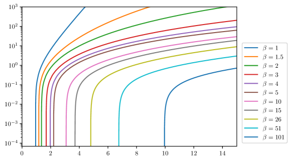
Figure 8: Logarithm of the position of the level line of height $\frac{1}{2}$ of numerical approximations of the solution to the problem with fractional diffusion, plotted as a function of time, for different values of $\beta$ and $s$ equal to $\frac{1}{2}$.

Conversely, Figures 9, 10 and 11 illustrate the different behaviours observed when the value of the parameter $s$ varies while the value of the parameter $\beta$ is fixed. For $\beta=1.5$, Figure 9 shows that acceleration occurs for any of the values of $s$ we considered, that is $s=0.3$, $0.5$, and $0.7$. For $\beta=3$, Figures 10 and 11 offer a more complex picture. In accordance with the theoretical prediction, one can observe a transition from an accelerated invasion for values of $s$ lower than $0.7$ to an invasion at constant speed for $s$ equal to $0.8$, the transition being captured for the value $s=0.75$. In both cases, it is observed that acceleration always occurs when $s<\frac{1}{2}$.

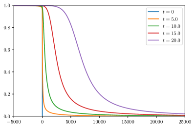
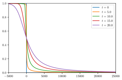
(a) $s=0.3$.

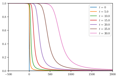
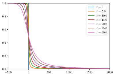
(b) $s=0.5$.

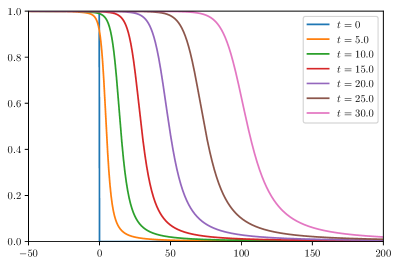
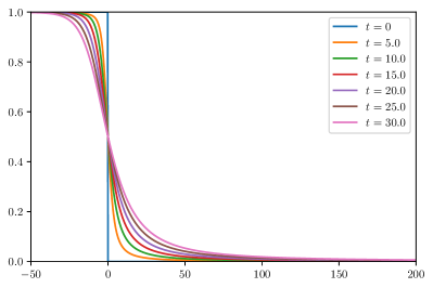
(c) $s=0.7$.

Figure 9: Numerical approximations of the solution to the problem with fractional diffusion at different times for $\beta=1.5$ and different values of $s$. On the right, the graphs have been shifted by setting the position of the level line of value $\frac{1}{2}$ at $x=0$, for comparison purposes.

The acceleration being more pronounced for small values of the parameter $s$, one may notice that the ranges used to plot the profiles of the solution vary drastically from a case to another, which may lead to some possible misinterpretations of the numerical results. There is for instance a factor $20$ between the range used for the case $s=0.3$ and the one for the case $s=0.5$. In order to properly compare the deformation of the profile, we have plotted in Figure 12 the shifted profile of the level set at a given time and for several values of $s$. By doing so, we are able to observe more easily the transition occuring at $s=0.75$, the profiles associated with values of $s$ greater than $0.75$ being very much alike whereas they exhibit a noticeable deformation for lower values.

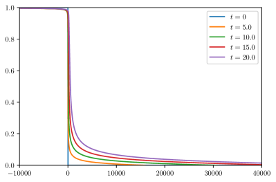
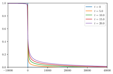
(a) $s=0.25$.

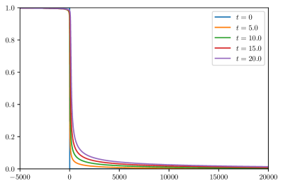
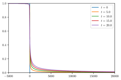
(b) $s=0.3$.

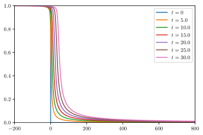
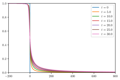
(c) $s=0.5$.

Figure 10: Numerical approximations of the solution to the problem with fractional diffusion at different times for $\beta=3$ and different values of the fractional Laplacian exponent $s$. On the right, the graphs have been shifted by setting the position of the level line of value $\frac{1}{2}$ at $x=0$, for comparison purposes.

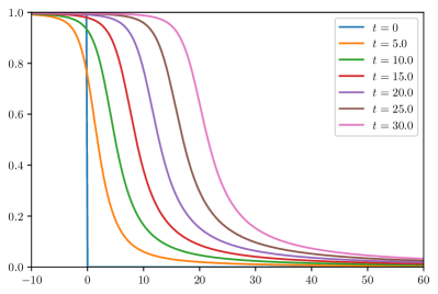
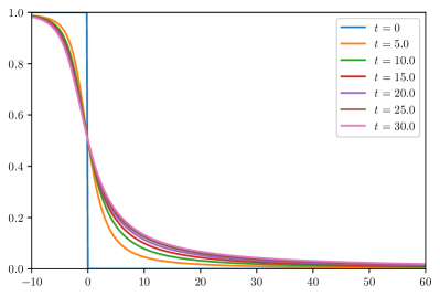
(a) $s=0.7$.

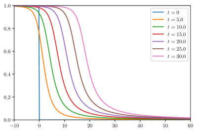
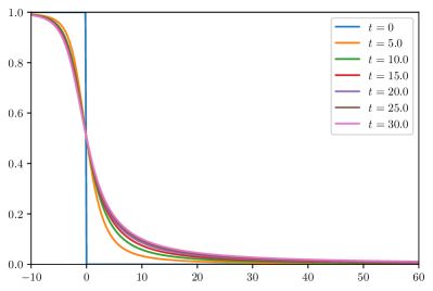
(b) $s=0.75$.

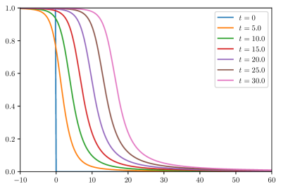
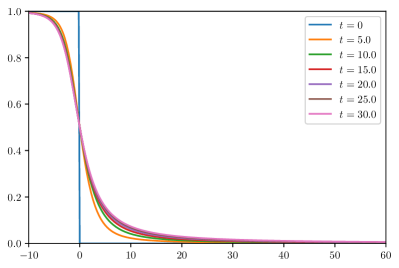
(c) $s=0.8$.

Figure 11: Numerical approximations of the solution to the problem with fractional diffusion at different times for $\beta=3$ and different values of $s$. On the right, the graphs have been shifted by setting the position of the level line of value $\frac{1}{2}$ at $x=0$, for comparison purposes.

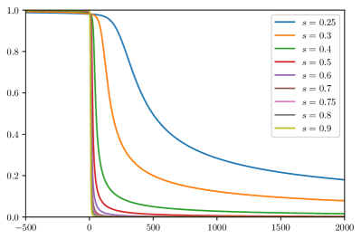
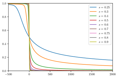
Figure 12: Numerical approximations of the solution to the problem with fractional diffusion at time $t=20$ for $\beta=3$ and different values of $s$. On the right, the graphs have been shifted by setting the position of the level line of value $\frac{1}{2}$ at $x=0$, for comparison purposes.

Lastly, we tried to fit a part of the profiles to the expected asymptotic behaviour of the solution at the front in Figure 13, in order to show that, despite the Dirichlet boundary conditions, one may still observe a decay behaving like $\frac{C}{x^{2s}}$ in the numerical solutions. This fitting was achieved with the method of least squares implemented in the scipy.optimize.curve_fit routine.

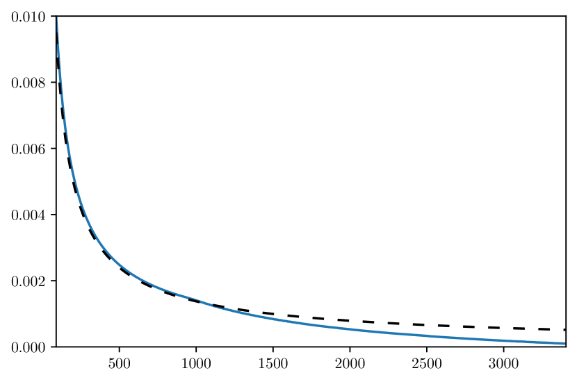
(a) $s=0.4$.

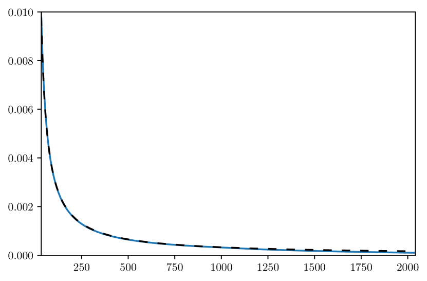
(b) $s=0.5$.

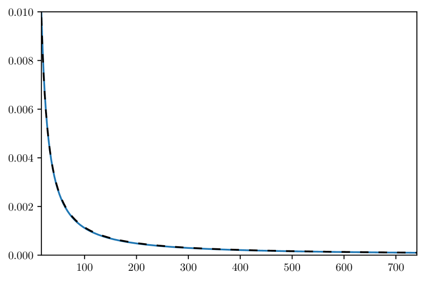
(c) $s=0.6$.

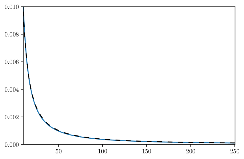
(d) $s=0.7$.

Figure 13: Fitting of the part of the tail of the approximation solution at time $t=1$ bounded by value $10^{-2}$ on the left and value $10^{-4}$ on the right using the function $\frac{C}{x^{2s}}$ for $\beta=1.5$ and different values of $s$.

References

- [1] G. Alberti and G. Bellettini. A nonlocal anisotropic model for phase transitions. I. The optimal profile problem. Math. Ann., 310(3):527–560, 1998.
- [2] M. Alfaro. Fujita blow up phenomena and hair trigger effect: the role of dispersal tails. Ann. Inst. H. Poincaré C, Anal. Non Linéaire, 34(5):1309–1327, 2017.
- [3] M. Alfaro. Slowing Allee effect versus accelerating heavy tails in monostable reaction diffusion equations. Nonlinearity, 30(2):687–702, 2017.
- [4] M. Alfaro and J. Coville. Propagation phenomena in monostable integro-differential equations: acceleration or not? J. Differential Equations, 263(9):5727–5758, 2017.
- [5] M. Alfaro and T. Giletti. Interplay of nonlinear diffusion, initial tails and Allee effect on the speed of invasions. arXiv:1711.10364 [math.AP], 2017.
- [6] M. Alfaro and T. Giletti. When fast diffusion and reactive growth both induce accelerating invasions. Comm. Pure Appl. Anal., 18(6):3011–3034, 2019.
- [7] W. C. Allee. The social life of animals. Norton, 1938.
- [8] D. G. Aronson and H. F. Weinberger. Multidimensional nonlinear diffusion arising in population genetics. Adv. in Math., 30(1):33–76, 1978.
- [9] U. M. Asher, S. J. Ruuth, and R. J. Spitteri. Implicit-explicit Runge–Kutta methods for time-dependent partial differential equations. Appl. Numer. Math., 25(2-3):151–167, 1997.
- [10] L. Berec, E. Angulo, and F. Courchamp. Multiple Allee effects and population management. Trends Ecol. Evol., 22(4):185–191, 2007.
- [11] R. M. Blumenthal and R. K. Getoor. Some theorems on stable processes. Trans. Amer. Math. Soc., 95(2):263–273, 1960.
- [12] K. Bogdan, T. Grzywny, and M. Ryznar. Density and tails of unimodal convolution semigroups. J. Funct. Anal., 266(6):3543–3571, 2014.
- [13] E. Bouin, J. Coville, and G. Legendre. Acceleration in integro-differential combustion equations. arXiv:2105.09946 [math.AP], 2021.
- [14] E. Bouin, J. Coville, and G. Legendre. Sharp exponent of acceleration in integro-differential equations with weak Allee effect. arXiv:2105.09911 [math.AP], 2021.
- [15] E. Bouin, J. Garnier, C. Henderson, and F. Patout. Thin front limit of an integro-differential Fisher-KPP equation with fat-tailed kernels. SIAM J. Math. Anal., 50(3):3365–3394, 2018.
- [16] J. Brasseur and J. Coville. Propagation phenomena with nonlocal diffusion in presence of an obstacle. J. Dynam. Differential Equations, pages 1–65, 2021.
- [17] X. Cabré and J.-M. Roquejoffre. The influence of fractional diffusion in Fisher-KPP equations. Comm. Math. Phys., 320(3):679–722, 2013.
- [18] X. Cabré and J.-M. Roquejoffre. Propagation de fronts dans les équations de Fisher-KPP avec diffusion fractionnaire. C. R. Math. Acad. Sci. Paris, 347(23-24):1361–1366, 2009.
- [19] J. Carr and A. Chmaj. Uniqueness of travelling waves for nonlocal monostable equations. Proc. Amer. Math. Soc., 132(8):2433–2439, 2004.
- [20] F. Courchamp, L. Berec, and J. Gascoigne. Allee effects in ecology and conservation. Oxford University Press, 2008.
- [21] J. Coville. On uniqueness and monotonicity of solutions of non-local reaction diffusion equation. Ann. Mat. Pura Appl. (4), 185(3):461–485, 2006.
- [22] J. Coville. Travelling fronts in asymmetric nonlocal reaction diffusion equations: the bistable and ignition cases. preprint hal-00696208, 2007.
- [23] J. Coville, J. Dávila, and S. Martínez. Nonlocal anisotropic dispersal with monostable nonlinearity. J. Differential Equations, 244(12):3080–3118, 2008.
- [24] J. Coville and L. Dupaigne. On a non-local equation arising in population dynamics. Proc. Roy. Soc. Edinburgh Sect. A, 137(4):727–755, 2007.
- [25] J. Coville, C. Gui, and M. Zhao. Propagation acceleration in reaction diffusion equations with anomalous diffusions. Nonlinearity, 34(3):1544–1576, 2021.
- [26] W. Cygan, T. Grzywny, and B. Trojan. Asymptotic behavior of densities of unimodal convolution semigroups. Trans. Amer. Math. Soc., 369(8):5623–5644, 2017.
- [27] B. Dennis. Allee effects: population growth, critical density, and the chance of extinction. Natur. Resource Modeling, 3(4):481–538, 1989.
- [28] S. Duo, H. W. van Wyk, and Y. Zhang. A novel and accurate finite difference method for the fractional Laplacian and the fractional Poisson problem. J. Comput. Physics, 355:233–252, 2018.
- [29] R. A. Fisher. The wave of advance of advantageous genes. Ann. Eugenics, 7(4):335–369, 1937.
- [30] J. Garnier. Accelerating solutions in integro-differential equations. SIAM J. Math. Anal., 43(4):1955–1974, 2011.
- [31] T. Grzywny, M. Ryznar, and B. Trojan. Asymptotic behaviour and estimates of slowly varying convolution semigroups. Internat. Math. Res. Notices, 2019(23):7193–7258, 2019.
- [32] C. Gui and T. Huan. Traveling wave solutions to some reaction diffusion equations with fractional Laplacians. Calc. Var. Partial Differential Equations, 54(1):251–273, 2015.
- [33] F. Hamel and L. Roques. Fast propagation for KPP equations with slowly decaying initial conditions. J. Differential Equations, 249(7):1726–1745, 2010.
- [34] Y. Huang and A. Oberman. Numerical methods for the fractional Laplacian: a finite difference-quadrature approach. SIAM J. Numer. Anal., 52(6):3056–3084, 2014.
- [35] G. Jaramillo, L. Cappanera, and C. Ward. Numerical methods for a diffusive class of nonlocal operators. J. Sci. Comput., 88:–, 2021.
- [36] K. Kaleta and P. Sztonyk. Spatial asymptotics at infinity for heat kernels of integro-differential operators. Trans. Amer. Math. Soc., 371(9):6627–6663, 2019.
- [37] J. R. King and P. M. McCabe. On the Fisher-KPP equation with fast nonlinear diffusion. Proc. Roy. Soc. London Ser. A, 459(2038):2529–2546, 2003.
- [38] A. N. Kolmogorov, I. G. Petrovskii, and N. S. Piscounov. Étude de l’équation de la diffusion avec croissance de la quantité de matière et son application à un problème biologique. Bull. Univ. Moscou, Ser. Internat.(Sect. A):1–25, 1937.
- [39] F. Lutscher, E. Pachepsky, and M. A. Lewis. The effect of dispersal patterns on stream populations. SIAM Rev., 47(4):749–772, 2005.
- [40] J. Medlock and M. Kot. Spreading disease: integro-differential equations old and new. Math. Biosci., 184(2):201–222, 2003.
- [41] V. Minden and L. Ying. A simple solver for the fractional Laplacian in multiple dimensions. SIAM J. Sci. Comput., 42(2):A878–A900, 2020.
- [42] R. Nathan, E. Klein, J. J. Robledo-Arnuncio, and E. Revilla. Dispersal kernels: review. In Dispersal ecology and evolution, pages 187–210. Oxford University Press, 2012.
- [43] A. P. Nield, R. Nathan, N. J. Enright, P. G. Ladd, and G. L. W. Perry. The spatial complexity of seed movement: animal-generated seed dispersal patterns in fragmented landscapes revealed by animal movement models. J. Ecology, 108(2):687–701, 2020.
- [44] S. Petrovskii, A. Mashanova, and V. A. A. Jansen. Variation in individual walking behavior creates the impression of a lévy flight. Proc. Nat. Acad. Sci. U.S.A., 108(21):8704–8707, 2011.
- [45] G. Pólya. On the zeros of an integral function represented by Fourier’s integral. Messenger Math., 52:185–188, 1923.
- [46] K. Schumacher. Travelling-front solutions for integro-differential equations. I. J. Reine Angew. Math., 1980(316):54–70, 1980.
- [47] D. Stan and J. L. Vázquez. The Fisher-KPP equation with nonlinear fractional diffusion. SIAM J. Math. Anal., 46(5):3241–3276, 2014.
- [48] X. Tian and Q. Du. Analysis and comparison of different approximations to nonlocal diffusion and linear peridynamic equations. SIAM J. Numer. Anal., 51(6):3458–3482, 2013.
- [49] H. F. Weinberger. Long-time behavior of a class of biological models. SIAM J. Math. Anal., 13(3):353–396, 1982.
- [50] H. Yagisita. Existence and nonexistence of travelling waves for a nonlocal monostable equation. Publ. Res. Inst. Math. Sci., 45(4):925–953, 2009.
- [51] G.-B. Zhang, W.-T. Li, and Z.-C. Wang. Spreading speeds and traveling waves for nonlocal dispersal equations with degenerate monostable nonlinearity. J. Differential Equations, 252(9):5096–5124, 2012.
- [52] Y. P. Zhang and A. Zlatoš. Optimal estimates on the propagation of reactions with fractional diffusion. arXiv:2105.12800 [math.AP], 2021.
- [53] A. Zlatoš. Quenching and propagation of combustion without ignition temperature cutoff. Nonlinearity, 18(4):1463–1476, 2005.