Many-electron character of two-photon above-threshold ionization of Ar

Abstract

The absolute generalized cross sections and angular distribution parameters of photoelectrons for the two-photon above threshold $3p$-ionization of Ar were calculated in the exciting photon energy range from 15.76 to 36 eV. The correlation function technique developed earlier was extended for the case when an intermediate-state function is of a continuum-type.

We show that two-photon ionization of Ar near the $3p^{4}$ threshold to a large extent is determined by the $(3p\dashrightarrow\varepsilon d)^{2}$ two-photon absorption via the giant resonance. This many-electron correlation causes (i) an increase of the photoionization cross sections by more than a factor of 3; (ii) the appearance of resonances in the exciting-photon energy range of the doubly-excited states. The predictions are supported by a good agreement between length and velocity results obtained after taking into account of the higher-order perturbation theory corrections.

I Introduction

Advancements in new intense and tunable free-electron lasers (FELs) ackermann07s ; shintake08s ; emma10s ; ishikawa12s ; kang17s covering the ultra-violet and X-ray photon-energy ranges inspire a renewed interest for a detailed comprehension of multi-photon processes. Experimental data obtained using FELs are of great motivation for theory to provide not only qualitative but also quantitative description of new phenomena.

One of these cases is atomic two-photon above-threshold ionization (ATI) when the energy of a single photon is sufficient to ionize an atom. It has been shown pindzola75 ; starace87 ; lhuillier87 ; pan90 ; petrov16 ; lagutin17 that below the one-photon ionization threshold many-electron correlations significantly influence the calculated cross sections and angular distribution parameters of photoelectrons with respect to those obtained in single-electron approximation. The intermediate-state shake-up correlation studied in pan90 ; petrov16 ; lagutin17 resulted in a noticeably closer agreement of the generalized two-photon ionization cross section (G2PICS) calculated in length (G2PICS-$L$) and velocity (G2PICS-$V$) forms of the electric dipole operator. The final-state electron scattering correlations taken into account in starace87 ; lhuillier87 ; petrov16 ; lagutin17 decrease noticeably the absolute values of G2PICS. In contrast, the polarization of the atomic core by the photoelectron petrov16 ; lagutin17 increases the cross sections by 15-20%.

To the best of our knowledge, there is only one ab initio theoretical description of the two-photon ATI of Ar pi10 . Those calculations were carried out using Herman-Skillman herman63 potential for computing atomic orbitals (AOs) without considering the collective behaviour of electrons.

In this work we intend to take into account many-electron correlations in the calculation of the $3p$-ATI of Ar. To solve this problem, the correlation function (CF) technique developed by us in petrov16 ; lagutin17 for the exciting-photon energy region below the one-photon ionization threshold is applied. We extent the CF technique for the ATI case solving two challenging problems: (i) computing the CFs for positive energy, i.e., in the continuum, satisfying the correct boundary conditions; (ii) computing the free-free dipole transition matrix elements containing the CF and final-state wave function, both of continuum-type.

The paper is organized as follows. In section II we describe the correlation function method for a two-photon transition amplitude calculation in the above-threshold exciting-photon energy region. The technique of the matrix element calculation for the two continuum-state functions is also described in detail. In section III the developed method is applied to the calculation of partial and total G2PICS of the $3p$ shell of Ar above the $3p$ threshold. Various correlation effects are considered and discussed. The influence of many-electron correlations on the angular-distribution parameters of the photoelectrons is studied in section IV. We conclude with a brief summary in section V.

II Two-photon transition amplitudes for the above-threshold photon energies

In order to investigate the influence of many-electron correlations on the ATI of atoms we considered the two-photon $3p$-ionization of argon applying the LS-coupling scheme:

$$\mathrm{Ar}~{}3p^{6}(^{1}S)+2\gamma\rightarrow\mathrm{Ar}~{}3p^{5}(^{2}P)\varepsilon\ell(^{1}L)\;\;\;\;\;(L=0;2).$$ (1)

Here $L$ and $\ell$ are the orbital angular momenta of the final state and photoelectron, respectively. We investigate the case when the energy of a single photon is sufficient to ionize the atom. This process is known as above-threshold ionization (ATI).

The amplitude of the two-photon ionization transition $i\rightarrow f$ with photon energy $\omega$ in the lowest order of perturbation theory (LOPT) in the ATI energy region is given by:

$$T_{i\rightarrow f}=\sum_{m}\frac{\left\langle f\left|D\right|m\right\rangle\left\langle m\left|D\right|i\right\rangle}{E_{i}+\omega-E_{m}+i\delta},\;\;\;\;\;\delta\rightarrow 0+$$ (2)

where $E_{i}$ and $E_{m}$ are energies of the initial and intermediate states respectively, $D$ is the electric dipole operator, $\delta$ is a infinitesimal positive quantity, and the sum contains all possible intermediate states $m$ including continuum ones. The contributions accounting for many-electron correlations were taken into account in addition to the LOPT amplitude (2). We study all possible correlations which are allowed in the next order of perturbation theory due to Coulomb interaction of electrons. These transitions can schematically be presented as shown below.

The LOPT processes are:

$$\begin{array}[c]{lcc}p^{6}\dashrightarrow p^{5}\varepsilon^{\prime}\ell^{\prime}\dashrightarrow p^{5}\varepsilon\ell&&(\text{Ia})\\ s^{2}p^{6}\dashrightarrow s^{1}p^{6}\varepsilon\ell\dashrightarrow s^{2}p^{5}\varepsilon\ell&&(\text{Ib})\end{array}$$

Here and below, the dash arrows denote electric dipole interaction and solid arrows - Coulomb interaction of electrons.

The correlations described by the next order of perturbation theory are classified as follows:

Intermediate-state interchannel correlation:

$$\begin{array}[c]{lcc}p^{6}\dashrightarrow p^{5}\varepsilon^{\prime\prime}\ell^{\prime\prime}\rightarrow p^{5}\varepsilon^{\prime}\ell^{\prime}\dashrightarrow p^{5}\varepsilon\ell&&(\text{II})\end{array}$$

Ground-state correlations:

$$\begin{array}[c]{lcc}p^{6}\rightarrow p^{4}\varepsilon^{\prime}\ell^{\prime}\varepsilon^{\prime\prime}\ell^{\prime\prime}\dashrightarrow p^{5}\varepsilon^{\prime}\ell^{\prime}\dashrightarrow p^{5}\varepsilon\ell&&(\text{IIIa})\\ p^{6}\rightarrow p^{4}\varepsilon^{\prime}\ell^{\prime}\varepsilon^{\prime\prime}\ell^{\prime\prime}\dashrightarrow p^{4}\varepsilon\ell\varepsilon^{\prime\prime}\ell^{\prime\prime}\dashrightarrow p^{5}\varepsilon\ell&&(\text{IIIb})\end{array}$$

$$\begin{array}[c]{lcc}p^{6}\rightarrow p^{4}\varepsilon\ell\varepsilon^{\prime\prime}\ell^{\prime\prime}\dashrightarrow p^{4}\varepsilon\ell\varepsilon^{\prime}\ell^{\prime}\dashrightarrow p^{5}\varepsilon\ell&&(\text{IIIc}).\end{array}$$

Intermediate-state shake-up correlation:

$$\begin{array}[c]{lcc}p^{6}\dashrightarrow p^{5}\varepsilon^{\prime}\ell^{\prime}\rightarrow p^{4}\varepsilon\ell\varepsilon^{\prime}\ell^{\prime}\dashrightarrow p^{5}\varepsilon\ell&&(\text{IV}).\end{array}$$

Intermediate-state electron scattering correlations:

$$\begin{array}[c]{lcc}p^{6}\dashrightarrow p^{5}\varepsilon^{\prime}\ell^{\prime}\rightarrow p^{4}\varepsilon\ell\varepsilon^{\prime\prime}\ell^{\prime\prime}\dashrightarrow p^{5}\varepsilon\ell&&(\text{V}).\end{array}$$

Final-state electron scattering correlations:

$$\begin{array}[c]{lcc}p^{6}\dashrightarrow p^{5}\varepsilon^{\prime}\ell^{\prime}\dashrightarrow p^{4}\varepsilon^{\prime}\ell^{\prime}\varepsilon^{\prime\prime}\ell^{\prime\prime}\rightarrow p^{5}\varepsilon\ell&&(\text{VIa})\\ p^{6}\dashrightarrow p^{5}\varepsilon^{\prime\prime}\ell^{\prime\prime}\dashrightarrow p^{4}\varepsilon^{\prime}\ell^{\prime}\varepsilon^{\prime\prime}\ell^{\prime\prime}\rightarrow p^{5}\varepsilon\ell&&(\text{VIb}).\end{array}$$

II.1 Correlation function for positive energy

The radial part of the amplitude for process (Ia) is

$$t_{\omega}^{(\text{Ia})}(L,\ell,\ell^{\prime})=\sum_{\varepsilon^{\prime}>F}\frac{\left\langle\varepsilon\ell\left|d_{r}\right|\varepsilon^{\prime}\ell^{\prime}\right\rangle\left\langle\varepsilon^{\prime}\ell^{\prime}\left|d_{r}\right|3p\right\rangle}{\omega-E_{3p}^{(i)}-\varepsilon^{\prime}+i\delta},$$ (3)

where $E_{\text{3p}}^{(i)}$ is the ionization potential of the $3p-$electron in Ar, $d_{r}$ is the radial part of the dipole transition operator obtained in the length or velocity form, and the notation $\varepsilon^{\prime}>F$ denotes the summation over all unoccupied single-electron states. The wave function of the photoelectron, $|\varepsilon\ell\rangle$, depends on the orbital momentum $L$ of the final state.

The infinite summation in (3) can be efficiently performed by the correlation-function (CF) method (petrov16 ; lagutin17 and references therein). In the ATI case, the CF should satisfy the outgoing-wave boundary conditions and it is a solution of the inhomogeneous integro-differential equation

$$\left(h_{\ell^{\prime}}-\omega+E_{3p}^{(i)}\right)\phi_{\ell^{\prime}}(r) =-d_{r}P_{3p}(r)$$

$$+\sum_{n^{\prime}<F}P_{n^{\prime}\ell^{\prime}}(r)\left\langle n^{\prime}\ell^{\prime}\left|d_{r}\right|3p\right\rangle,$$ (4)

where $h_{\ell^{\prime}}$ is the Hartree-Fock operator for the $\varepsilon^{\prime}\ell^{\prime}$ function in the configuration $3p^{5}\varepsilon^{\prime}\ell^{\prime}(^{1}P)$.

In order to obtain the continuum-type CF, we have used the technique similar to that presented in Robicheaux93 . First, the inhomogeneous equation (4) is solved disregarding the boundary conditions at large distances ($r\rightarrow\infty$). This solution, which we denote $\Lambda_{l^{\prime}}$, has a nonzero contribution from the incoming waves, and its asymptotic behaviour at ($r\rightarrow\infty$) can be expressed as

$$\Lambda_{l^{\prime}}(r)=gG(r)+hH(r),$$ (5)

where $G(r)$ and $H(r)$ are regular and irregular Coulomb functions, respectively curtis64 , asymptotically denoted as

$$G_{\varepsilon\ell}(r)\overset{r\rightarrow\infty}{\longrightarrow}\sqrt{\frac{2}{\pi k}}\sin\left(kr-\frac{\ell\pi}{2}+\frac{Z}{k}\mathrm{ln}(2kr)+\delta_{\ell}\right),$$ (6)

$$H_{\varepsilon\ell}(r)\overset{r\rightarrow\infty}{\longrightarrow}-\sqrt{\frac{2}{\pi k}}\cos\left(kr-\frac{\ell\pi}{2}+\frac{Z}{k}\mathrm{ln}(2kr)+\delta_{\ell}\right).$$ (7)

Here, $k$ is the wave vector of the continuum electron in atomic units, $Z$ is the asymptotic charge of the ionic core, $\delta_{\ell}$ represents the sum

$$\delta_{\ell}=\mathrm{arg}~{}\Gamma\left(\ell+1-\imath\frac{Z}{k}\right)+\varphi_{\ell},$$ (8)

where $\varphi_{\ell}$ is the short-range phase shift. Coefficients $g$ and $h$ in (5) are defined by matching the respective numerical solutions of inhomogeneous Eq. (4) starting upward from zero and downward from infinity.

In order to obtain the solution of Eq. (4), which has the correct boundary condition appropriate for the photoionization case, we add the general solution $P_{\varepsilon^{\prime}\ell^{\prime}}(r)$ of the homogeneous equation to $\Lambda_{l^{\prime}}(r)$, factorized with a coefficient $A$

$$\left(h_{\ell^{\prime}}-\omega+E_{3p}^{(i)}\right)P_{\varepsilon^{\prime}\ell^{\prime}}(r)=0.$$ (9)

The solution of Eq. (4), which has the correct boundary conditions, is thus given by:

$$\phi_{l^{\prime}}(r)=\Lambda_{l^{\prime}}(r)+A\,P_{\varepsilon^{\prime}\ell^{\prime}}(r),$$ (10)

where $\Lambda_{l^{\prime}}(r)$ is the solution (5) of Eq. (4) with unphysical boundary conditions.

The solution of the homogeneous equation (9) in its asymptotics ($r\rightarrow\infty$) can be determined as

$$P_{\varepsilon^{\prime}\ell^{\prime}}(r)=G(r)-K\,H(r),$$ (11)

where the coefficient $K$ is obtained by matching the respective numerical solutions of Eq. (9) starting upward from zero and downward from infinity.

Substituting Eqs. (5) and (11) into (10), applying the Euler expressions $\sin x=\frac{i}{2}(e^{-ix}-e^{ix})$ and $\cos x=\frac{1}{2}(e^{-ix}+e^{ix})$ with $x={kr-\frac{\ell\pi}{2}+\frac{Z}{k}\mathrm{ln}(2kr)+\delta_{\ell}}$, and equating a factor at $e^{-ix}$ to zero, we obtain the following formulae for the coefficient $A$ in Eq. (10):

$$\mathrm{Re}\;A=-\frac{hK+g}{K^{2}+1};~{}~{}~{}~{}~{}~{}~{}~{}\mathrm{Im}\;A=\frac{gK-h}{K{{}^{2}}+1}.$$ (12)

After the CF is determined in the form of (10), the radial part of the transition amplitude (3) takes the following form:

$$t_{q,\omega}^{(\text{Ia})}(L,\ell,\ell^{\prime})=\left\langle\varepsilon\ell\left|d_{r}\right|\phi_{\ell^{\prime}}\right\rangle.$$ (13)

II.2 Calculation of electric dipole transition amplitude between two continuum-type functions

In Eq.(13) both the CF, $\phi_{\ell^{\prime}}(r)$, and the final-state AO, $P_{\varepsilon\ell}(r)$, are of continuum-type. In order to calculate the dipole integral (13) between the two continuum wave functions, a special technique was applied. We used the method described in aymar80 ; gao87 . According to this method, the dipole integral (13) is expressed as

$$\left\langle\varepsilon\ell\right|d_{r}\left|\phi_{\ell^{\prime}}\right\rangle=\int_{0}^{r_{0}}P_{\varepsilon\ell}(r)\;d_{r}\;\phi_{\ell^{\prime}}(r)dr+I(r_{0},\varepsilon\ell,\varepsilon^{\prime}\ell^{\prime}),$$ (14)

where $r_{0}$ is a sufficiently large value of $r$ and

$$I(r_{0},\varepsilon\ell,\varepsilon^{\prime}\ell^{\prime})=\int_{r_{0}}^{\infty}u_{\varepsilon\ell}(r)\;d_{r}\;u_{\varepsilon^{\prime}\ell^{\prime}}(r)dr.$$ (15)

The radial functions $u_{\varepsilon\ell}(r)$ in (15) are the standard Coulomb functions which are the solutions of the equation

$$\left(\frac{d^{2}}{dr^{2}}+f_{\ell}(r)\right)u_{\varepsilon\ell}(r)=0,\\ f_{\ell}(r)=k^{2}+\frac{2Z}{r}-\frac{\ell(\ell+1)}{r^{2}},~{}~{}~{}(r\geq r_{0}),$$ (16)

where $\varepsilon\text{(Ry)}=k^{2}$.

The solutions of Eq. (16) are asymptotically expressed as

$$u_{\varepsilon\ell}(r)=\sqrt{\frac{2}{\pi\xi_{\ell}(r)}}\sin\left(\Phi_{\ell}^{(1)}(r)+\delta_{\ell}\right).$$ (17)

In Eq. (17), an approximate value of $\Phi_{\ell}^{(1)}(r)$ with an accuracy of $1/r^{4}$ can be obtained using the formulae presented in aaberg82 ; burgess63 :

$$\Phi_{\ell}^{(1)}=x+\frac{1}{m}\ln\left(\frac{1}{m}+mp+x\right)-\frac{1}{m}-\frac{\ell\pi}{2}\\ +y-\frac{x\left(3m^{2}t+4\right)+m\rho\left(3m^{2}+2\right)+mt}{24\left(1+m^{2}t\right)\rho}\\ +\frac{5\left(\rho-t\right)}{24x^{3}},$$ (18)

where the abbreviations $m=k/Z$, $\rho=Zr$, $x=\left(m^{2}\rho^{2}+2\rho-t\right)^{1/2}$, $t=\ell(\ell+1)$ and

$$y=\left\{\begin{array}[c]{c}\frac{t+1/8}{\sqrt{t}}\arccos\left[\frac{\rho-t+mtx}{\left(1+m^{2}t\right)\rho}\right],\;\;l>0;\\ \frac{1}{4\left(x+m\rho\right)},\;\;\;l=0.\end{array}\right.$$ (19)

are used. Note that in aaberg82 there is a misprint in the definition of $x$, whereas in burgess63 there is a misprint in Eq. (18).

The amplitude function $\xi_{\ell}(r)$ appearing in Eq. (17), satisfies the following differential equation

$$\xi_{\ell}^{2}(r)=f_{\ell}(r)+\xi_{\ell}^{1/2}(r)\frac{d^{2}}{dr^{2}}\xi_{\ell}^{-1/2}(r).$$ (20)

Equation (20) can be solved iteratively. A zeroth approximation is expressed as $\xi_{\ell}^{(0)}(r)=\sqrt{f_{\ell}}$. The next approximation can be calculated by aaberg82

$$\xi_{\ell}^{(1)}=\sqrt{f_{\ell}+\xi_{\ell}^{1/4}\frac{d^{2}}{dr^{2}}\xi_{\ell}^{-1/4}}\\ =\sqrt{f_{\ell}+\frac{5}{16}\left(\frac{f_{\ell}^{\prime}}{f_{\ell}}\right)^{2}-\frac{1}{4}\frac{f_{\ell}^{\prime\prime}}{f_{\ell}}}.$$ (21)

Integral (15) can be expressed as a difference of two terms:

$$I(r_{0},\varepsilon\ell,\varepsilon^{\prime}\ell^{\prime})=I^{+}-I^{-},$$ (22)

where

$$I^{\pm}=\underset{\epsilon\rightarrow 0}{\lim}\int_{r_{0}}^{\infty}e^{-\epsilon r}\xi^{\pm}(r)g^{\pm}(r)\cos\chi^{\pm}(r)dr,$$ (23)

$$\xi^{\pm}(r)=\xi_{\ell^{\prime}}^{(1)}(r)\pm\xi_{\ell}^{(1)}(r),$$ (24)

$$g^{\pm}(r)=d_{r}\left[\pi\left(\xi_{\ell^{\prime}}^{(1)}\xi_{\ell}^{(1)}\right)^{1/2}\xi^{\pm}\right]^{-1},$$ (25)

$$\chi^{\pm}(r)=\left[\Phi_{\ell^{\prime}}^{(1)}+\delta_{\ell^{\prime}}\right]\pm\left[\Phi_{\ell}^{(1)}+\delta_{\ell}\right].$$ (26)

After subsequent integration of Eq. (23) by parts, the following expansion can be obtained gao87 :

$$I^{\pm}=\left\{\sum_{n=0}^{\infty}\left[\left(\frac{1}{\xi^{\pm}}\frac{d}{dr}\right)^{n}g^{\pm}(r)\right]\sin\left(\chi^{\pm}(r)+\frac{n\pi}{2}\right)\right\}_{r=r_{0}}.$$ (27)

In the present calculation we included the first four terms of expansion (27).

II.3 Additional computational remarks

The wave functions of the atomic core of Ar were computed on the ground-state configuration $1s^{2}2s^{2}2p^{6}3s^{2}3p^{6}$ obtained in the Hartree-Fock (HF) approximation. The final-state wave functions were obtained by solving the HF equations for a photoelectron in the configurations $3p^{5}\varepsilon p(^{1}S),3p^{5}\varepsilon p(^{1}D)$ and $3p^{5}\varepsilon f(^{1}D)$ using frozen core functions. The same frozen core functions were used in the $h_{\ell^{\prime}}$ operator in Eq. (4).

The Hartree-Fock operator entering Eq. (4) includes the non-local exchange part of the Coulomb interaction of the CF with core electrons. In the same way as in petrov16 , a separate local differential equation is determined for each term of the exchange Coulomb potential. As a result, the single non-local integro-differential equation (4), is transformed to a system of local differential equations. In order to solve this system a non-iterative numerical procedure is applied which is stable and converges at each energy.

The calculation of the transition amplitude (Ib) via the $3s$ shell is identical for above (ATI) and below threshold ionization. The latter case has been described in our previous work petrov16 . The correlation transition amplitudes (II)-(V) were calculated using the CF technique. The respective inhomogeneous equations were presented and discussed in petrov16 . In the ATI energy region, the calculations of the CFs are different in two cases. First, if the energy denominator in the expression for the transition amplitude has no pole, then the corresponding CF is of discrete-type, consists of a real part only, and is calculated using technique petrov16 . Second, in the case the energy denominator has a pole, then the CF is of continuum-type, consists of real and imaginary parts, and is computed using the method described above.

III Generalized two-photon ionization cross section for above-threshold ionization of the 3p shell of Ar

In order to characterize two-photon ionization quantitatively, we use the generalized two-photon ionization cross section (G2PICS) as defined in starace87 ; pan90 ; petrov16 . This intrinsic quantity does not contain the exciting-photon flux and is therefore ideally suited to characterize this process. The expression for the G2PICS is:

$$\sigma_{q}(\omega)=\sum_{L,\ell}\sigma_{q}(L,\ell,\omega),$$ (28)

where $q=0$ and $q=\pm 1$ correspond to a linearly or circularly polarized incoming radiation, respectively. Each partial generalized cross section is determined in cm${}^{4}~{}$s and expressed via the two-photon transition amplitudes $T_{q,\omega}(L,\ell)$ petrov16 as

$$\sigma_{q}(L,\ell,\omega)=\frac{8\pi^{3}\alpha a_{0}^{5}}{c}\omega^{\pm 2}\left|T_{q,\omega}(L,\ell)\right|^{2}.$$ (29)

In Eq. (29), $\alpha=1/137.036$ is the fine-structure constant; $a_{0}=5.29177\cdot 10^{-9}~{}$cm is the Bohr radius; $c=2.99792\cdot 10^{10}$ cm/s is the light velocity in vacuum; $\omega$ is the exciting photon energy in atomic units; ‘$+$’ and ‘$-$’ correspond to the length and velocity form of the electric dipole transition operator. The major details of the transition amplitude calculation (particularly the calculation of the angular parts) has been described in our previous work petrov16 .

III.1 LOPT approximation

The G2PICS of the $3p$ shell of Ar calculated in LOPT approximation (processes (Ia) and (Ib)) are presented in Fig. 1 in the exciting-photon energy region below the one-photon ionization threshold (our calculation from petrov16 ) and in ATI region (present calculation). In the same figure, the results of the G2PICS of Ar computed in pi10 in the LOPT approach is also depicted.

The total G2PICS have been plotted in pi10 vs the energy $\varepsilon_{1}=-\left|\varepsilon_{3p}\right|+\omega$ of the electron in the intermediate state. In our calculation the G2PICS is presented as functions of the exciting-photon energy $\omega$. To compare our data with the data of pi10 we used the experimental one-photon ionization potential of the $3p$-electron $E_{3p}^{(i)}=1.158$ Ry (corresponding to the energy level $E(^{2}P_{3/2})=15.7596$ eV kramida14 ) instead of the Herman-Skillman value $\left|\varepsilon_{3p}\right|=1.065$ Ry used in pi10 . This aligns the one-photon ionization thresholds in both calculations (see hatched line at 15.76 eV in Fig. 1).

The G2PICS obtained in pi10 agree fairly well with our calculation close to the two-photon ionization threshold ($\omega=7.8798$ eV). The data of pi10 is located between our G2PICS-$L$ and G2PICS-$V$ and differs from our G2PICS-$L$ by 15%. The deviation is larger in the ATI region, as seen from Fig. 1. At the one-photon $3p^{5}$ threshold, the cross section from pi10 exceeds our G2PICS-$L$ by more than three times, whereas at high photon energies it decreases more rapidly than our G2PICS, after $\omega=30$ eV it is close to the present G2PICS-$V$. We suggest that this disagreement arises most likely from the different approximations in the CFs calculation: Herman-Skillman in pi10 vs term-dependent Hartree-Fock 3$p^{5}\phi_{\ell^{\prime}}(^{1}\text{P})$ in the present work.

In order to support this suggestion we performed a separate study by calculating the G2PICS in the LOPT approach using the average self-consistent $3p^{5}\varepsilon^{\prime}\ell^{\prime}$ configuration instead of the term-dependent frozen core $3p^{5}\varepsilon^{\prime}\ell^{\prime}(^{1}P)$ configuration. In this case the present cross sections became closer to those obtained in pi10 .

The value of amplitude (Ib) for the transition via the $3s$ shell is less than 0.1% of the amplitude (Ia) and has practically no influence on the calculated cross section.

The results depicted in Fig. 1 show that the G2PICS calculated in our work in LOPT approximation in the length and velocity forms differ from each other by approximately two times. This difference indicates the necessity to include many-electron correlation in the calculation.

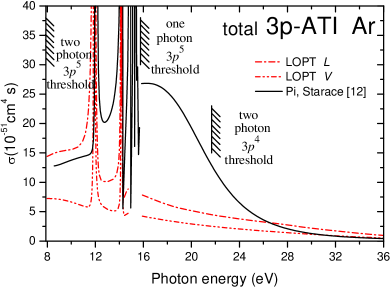
Figure 1: The 3$p$ shell total G2PICS in length ($L$) and velocity ($V$) form for linearly polarized incoming radiation calculated in LOPT below the one-photon 3$p$ threshold petrov16 and in the ATI region (present work). The calculation of pi10 is also presented for comparison (see text). The two-photon $3p^{5}(^{2}P_{3/2})$ and $3p^{4}(^{3}P_{2})$ thresholds from kramida14 are depicted as hatched lines.

III.2 Correlation processes of third order of perturbation theory

The total two-photon ionization cross section of the $3p$ shell of Ar is a sum of three partial cross sections for the transitions to the $\varepsilon p(^{1}S)$, $\varepsilon p(^{1}D)$ and $\varepsilon f(^{1}D)$ channels. As in pi10 , the $\varepsilon f(^{1}D)$ channel is found to dominate in the ATI region: in LOPT approximation at the one-photon $3p^{5}$ threshold the partial $\varepsilon f(^{1}D)$ cross sections are about 85% and 89% of the total 3$p$ cross sections in the length and velocity gauge, respectively. Therefore, the influence of many-electron correlations will be demonstrated here in detail for the case of the $\varepsilon f(^{1}D)$ channel only.

In Fig. 2, the partial G2PICS for the $\varepsilon f(^{1}D)$ channel calculated in LOPT are compared with the cross section computed with accounting for the processes (I)–(V) (correlation (VI) is excluded). The starting value of the photon energy corresponds to the one-photon $3p^{5}$-ionization threshold $\omega=15.7596$ eV. In Fig. 2, it is seen that the correlative transitions (II)-(V) change the G2PICS only quantitatively but without any qualitative change in their energy dependence.

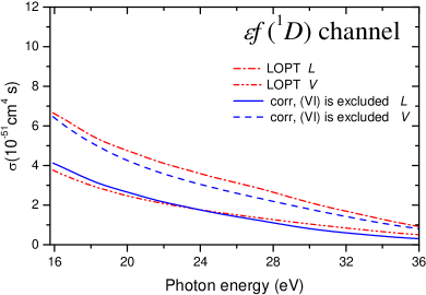
Figure 2: Partial G2PICS for the transition to the $3p^{5}\varepsilon f(^{1}D)$ channel, computed in length ($L$) and velocity ($V$) form for linearly polarized incoming radiation in LOPT and with accounting for transitions (I)-(V) (corr (VI) is excluded).

It turned out that in $3p$-ATI correlation correction (VI) is much more important than below the one-photon $3p$ threshold. In ATI, the transition amplitude (VI) is substantially (one order of magnitude) larger than the other correlation amplitudes (II)–(V) and changes the computed cross sections drastically. In the processes (VIa) and (VIb), the first and the second photon excite a pair of $3p$ core electrons to virtual $\varepsilon^{\prime}\ell^{\prime}$ and $\varepsilon^{\prime\prime}\ell^{\prime\prime}$ states; then because of the Coulomb interaction, one electron returns to the core and another changes the state to the $\varepsilon\ell$ final one. The large value of this correlation can be explained through the existence of the giant resonance in each of the single-electron $\left\langle\varepsilon d\left|d_{r}\right|3p\right\rangle$ transition amplitudes.

The radial part of the transition amplitude (VI) is described by the following expression:

$$t_{\omega}^{(\text{VIa,b})}(L,\ell,\ell^{\prime},\ell^{\prime\prime})=\\ =\sum_{\varepsilon^{\prime},\varepsilon^{\prime\prime}>F}\underset{k}{\sum}\left[a_{k}R^{k}(\varepsilon\ell 3p,\varepsilon^{\prime}\ell^{\prime}\varepsilon^{\prime\prime}\ell^{\prime\prime})\right.\\ \left.+b_{k}R^{k}(\varepsilon\ell 3p,\varepsilon^{\prime\prime}\ell^{\prime\prime}\varepsilon^{\prime}\ell^{\prime})\right]\left\langle\varepsilon^{\prime\prime}\ell^{\prime\prime}\left|d_{r}\right|3p\right\rangle\left\langle\varepsilon^{\prime}\ell^{\prime}\left|d_{r}\right|3p\right\rangle\\ \times\left\{\frac{1}{(2\omega-E_{3p^{2}}^{(i)}-\varepsilon^{\prime}-\varepsilon^{\prime\prime})(\omega-E_{3p}^{(i)}-\varepsilon^{\prime})}\right.\\ \left.+\frac{1}{(2\omega-E_{3p^{2}}^{(i)}-\varepsilon^{\prime}-\varepsilon^{\prime\prime})(\omega-E_{3p}^{(i)}-\varepsilon^{\prime\prime})}\right\},$$ (30)

where $E_{3p^{2}}^{(i)}$ $=3.189$ Ry is the experimental $43.3893$ eV kramida14 energy of the $3p^{4}(^{3}P_{2})$ level. The $a_{k}$ and $b_{k}$ are numerical coefficients given in petrov16 , and $R^{k}(\varepsilon\ell 3p,\varepsilon^{\prime}\ell^{\prime}\varepsilon^{\prime\prime}\ell^{\prime\prime})$ is the Slater integral

$$R^{k}(n_{1}\ell_{1},n_{3}\ell_{3};n_{2}\ell_{2},n_{4}\ell_{4})=\\ =\int_{0}^{\infty}P_{n_{3}\ell_{3}}(r)P_{n_{4}\ell_{4}}(r)y_{k}(P_{n_{1}\ell_{1}},P_{n_{2}\ell_{2}};r)dr,$$ (31)

$$y_{k}(P_{n_{1}\ell_{1}},P_{n_{2}\ell_{2}};r)=\int_{0}^{\infty}\frac{r_{<}^{k}}{r_{>}^{k+1}}P_{n_{1}\ell_{1}}(r^{\prime})P_{n_{2}\ell_{2}}(r^{\prime})dr^{\prime},$$ (32)

where $r_{<}$ and $r_{>}$ is the smaller and the larger of the radial coordinates $r$ and $r^{\prime}$.

Since the first factor in the denominator of the two terms in the curly braces of Eq. (30) contains both the $\varepsilon^{\prime}$ and $\varepsilon^{\prime\prime}$ intermediate state energies, the amplitude (30) cannot be expressed via CFs. In petrov16 , we followed the approximation of pan90 . In the first factor of the first fraction in curly braces containing $2\omega$, we replaced $\varepsilon^{\prime}$ by $\varepsilon^{\prime\prime}$ whereas in the second fraction in curly braces, we replaced $\varepsilon^{\prime\prime}$ by $\varepsilon^{\prime}$. After this assumption, Eq. (30) was simplified and expressed via the correlation functions. We estimated that at the near-threshold two-photon $3p$-ionization region the error of the approximated amplitude did not exceed 7% with respect to the data obtained using the exact expression (30).

The electron-scattering correlation (VI) is found to be very important in the ATI region. Therefore, we calculated it without the approximation discussed above using the exact expression (30). This was possible in this special case because in Eq. (30) both the Slater integrals $R^{k}(\varepsilon\ell 3p,\varepsilon^{\prime\prime}\ell^{\prime\prime}\varepsilon^{\prime}\ell^{\prime})$ and the dipole integrals $\left\langle\varepsilon^{\prime}\ell^{\prime}\right|d_{r}\left|3p\right\rangle$ and $\left\langle\varepsilon^{\prime\prime}\ell^{\prime\prime}\right|d_{r}\left|3p\right\rangle$ are not divergent due to the presence of a localized $3p$ function. To perform the summation in Eq. (30) over the $\varepsilon^{\prime}\ell^{\prime}$ and $\varepsilon^{\prime\prime}\ell^{\prime\prime}$, several discrete states and the continuum states up to 20 Ry were taken into account.

In Fig. 3, partial GSPICS for the transition to the $3p^{5}\varepsilon f(^{1}D)$ channel calculated considering the correlations (II)-(V) only and with all correlations (II)-(VI) are compared. A drastic difference between the two results is evident: (i) the G2PICS in length form is enhanced by an order of magnitude resulting in a pronounced maximum at $\omega=32$ eV; (ii) the correlation (VI) gives rise to doubly-excited state resonances below the two-photon $3p^{4}$ double-ionization threshold. The resonances become apparent at those photon energies when the denominators in Eq. (30) containing $2\omega$ are vanishing. The first, energetically lowest 3$p^{4}3d4s$ resonance in the partial $3p^{5}\varepsilon f(^{1}D)$ G2PICS is shown in Fig. 3. We restricted our presentation to this resonance because the precise calculation of the doubly-excited state energies is a cumbersome problem on its own (see, e.g., sukhorukov92 ; sukhorukov94a ; kammer06 ). The energies of the respective doubly-excited state resonances are expected to be larger than they appear in the relaxed $3p^{4}n^{\prime}\ell^{\prime}n^{\prime\prime}\ell^{\prime\prime}$ configuration. The two-photon double-ionization threshold equals to $0.5E_{3p^{2}}^{(i)}$ is depicted in Fig. 3 by the hatched line. It indicates the upper limit of the doubly-excited state resonances.

The revealed strong influence of many electron correlations on G2PICS including the resonance structure is beyond a simple single-electron picture of two-photon ionization and its experimental verification is of great fundamental importance.

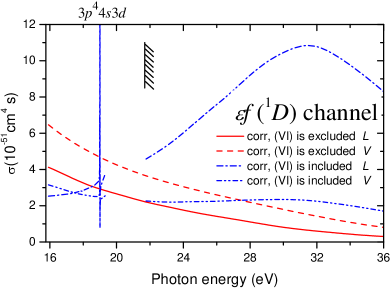
Figure 3: Partial G2PICS for the transition to the $3p^{5}\varepsilon f(^{1}D)$ channel, computed in length ($L$) and velocity ($V$) form for linearly polarized incoming radiation with accounting for transitions (I)-(V) (corr, (VI) is excluded) and with accounting for all correlations (I)-(VI) (corr, (VI) is included). The two-photon $3p^{4}(^{3}P_{2})$ ionization threshold is indicated by the hatched line. We show the energetically lowest calculated $3p^{4}4s3d$ doubly-excited state resonance only.

III.3 Many-electron correlations of higher orders of perturbation theory

G2PICS calculated in length and velocity gauges considering all the transitions (I)-(VI) still differ substantially, as it is seen from Fig. 3. At $\omega=32$ eV the G2PICS-$L$ (dashed-dotted line) is four times larger than G2PICS-$V$ (dash-double-dotted line). In our work, petrov16 a good agreement between computed G2PICS-$L$ and G2PICS-$V$ was achieved after inclusions of higher-order PT correlations. Those effects were: (i) the polarization of the atomic core by the photoelectron and (ii) the correlational decrease of the Coulomb interaction in the description of the correlative processes (II)-(VI). Additional calculations showed that in ATI region taking into account these higher-order PT correlations (i)-(ii) is not sufficient to make an agreement between G2PICS-$L$ and G2PICS-$V$ close. The reason is the anomalously large contribution of the correlation (VI) discussed above. In the present work, we take into account intrashell correlations amusia75 in addition to correlations (i)-(ii) when computing the matrix elements $\left\langle\varepsilon^{\prime}\ell^{\prime}\right|d_{r}\left|3p\right\rangle$ and $\left\langle\varepsilon^{\prime\prime}\ell^{\prime\prime}\right|d_{r}\left|3p\right\rangle$.

The ab initio core polarization potential $V^{CP}(r)$ petrov99 was included in the HF operator $h_{\ell^{\prime}}(r)$ entering the equations for the CFs and for the final-state electrons. In addition, the matrix elements of the Coulomb interaction describing the correlations (II)-(VI) have been reduced by a factor of 1.25 petrov16 . Here and below, the calculation with taking into account the processes (I)-(VI), intrashell correlations, polarization of the atomic core by the photoelectron and the correlational decrease of the Coulomb interaction will be designated as the configuration interaction Hartree-Fock approach with core polarization (CIHFCP).

The CIHFCP partial cross sections for the $\varepsilon f(^{1}D)$ channel are depicted in Fig. 4 (solid and dashed curves for length and velocity form, respectively). In the same figure the cross sections calculated with taking into account processes (I)-(VI) but without higher-order PT corrections are also presented (dash-dotted and dash-double-dotted curves) for comparison. It is clearly seen that accounting for higher-order PT corrections results in a very close agreement between the G2PICS-$L$ and G2PICS-$V$ both above the two-photon double-ionization threshold (to the right of the hatched line in Fig. 4) and in the region of the $3p^{4}4s3d$ resonance. The following changes in the calculated G2PICS can be seen from Fig. 4:

(i) the energy of the $3p^{4}4s3d$ resonance shifted by 0.15 eV to the low-energy side. The reason of the shift is the polarization of the atomic core by the photoelectron which decreases energies of the excited electrons;

(ii) the G2PICS becomes larger on the one-photon threshold ($\omega=15.76$ eV) by about 2 times;

(iii) maximum in the $\sigma(\omega)$ dependence above the two-photon $3p^{4}$ threshold is now shifted by $\sim 6$ eV to the low-energy side.

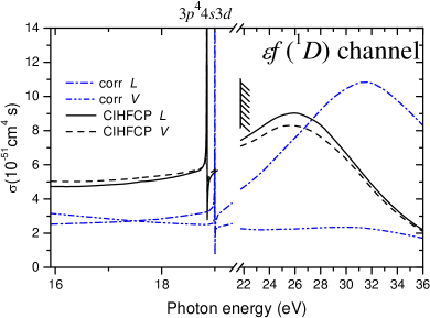
Figure 4: Partial G2PICS for the transition to the $3p^{5}\varepsilon f(^{1}D)$ channel, computed in length ($L$) and velocity ($V$) form for linearly polarized incoming radiation with accounting for all the correlations (I)-(VI) (corr) and, in addition, the higher-order PT correlations (CIHFCP). The two-photon $3p^{4}(^{3}P_{2})$ ionization threshold is indicated by the hatched line. The first calculated $3p^{4}4s3d$ doubly-excited state resonance is shown only.

The computed partial G2PICSs for the transitions to the $3p^{5}\varepsilon p(^{1}D)$ and $3p^{5}\varepsilon p(^{1}S)$ channels are depicted in Figs. 5a and 5b, respectively. Dash-dotted and dash-double-dotted lines represent results computed in the LOPT and solid and dashed lines represent CIHFCP results. Similar to the $3p^{5}\varepsilon f(^{1}D)$ channel, one can recognize a strong increase the G2PICSs, the appearance of the doubly-excited state resonances and a better agreement between length an velocity form results.

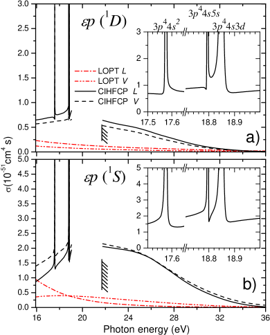
Figure 5: Partial G2PICS for the transitions to the $3p^{5}\varepsilon p(^{1}D)$ channel (a) and to the $3p^{5}\varepsilon p(^{1}S)$ channel (b), computed in length ($L$) and velocity ($V$) form for linearly polarized incoming radiation in LOPT and with taking into account both the correlations (I)-(VI) and higher-order PT correlations (CIHFCP). The two-photon $3p^{4}(^{3}P_{2})$ ionization threshold is indicated by the hatched line.

In the insets of Figs. 5a,b the doubly-excited state resonance region of the G2PICS-$L$ is presented on an enlarged scale. For the $3p^{5}\varepsilon f(^{1}D)$ channel, the lowest resonance corresponds to the $3p^{4}4s3d$ state (see Figs.3 and 4), whereas in the $3p^{5}\varepsilon p(^{1}D)$ and $3p^{5}\varepsilon p(^{1}S)$ channels the $3p^{4}4s^{2}$ and $3p^{4}4s5s$ states are also present. As it was already mentioned, precise calculation of the resonance energies is a separate cumbersome problem. In more detail, in the present calculation the energy of the $4s$ electron is equal to $\varepsilon_{4s}=-0.303$ Ry. When using the experimental value of the ionization potential $E_{3p^{2}}^{(i)}=3.189$ Ry, the first terms in both denominators in Eq. (30) are vanishing at $\omega=0.5\,E_{3p^{2}}^{(i)}+\varepsilon_{4s}=17.57$ eV. This energy corresponds to the position of the $3p^{4}4s^{2}$ resonance in Fig. 5. The experimental energy of the $3p^{4}4s^{2}$ resonance is at $\omega=13.475$ eV jorgensen78 . The main reason for this discrepancy is the approximate (frozen-core) value of $\varepsilon_{4s}$.

In pan90 ; petrov16 ; lagutin17 , a large influence of the intermediate-state shake-up (IV) correlation on the computed G2PICS was revealed, particularly on the $3p^{5}\varepsilon p(^{1}S)$ partial cross section. In the ATI case, this influence is of similar size, as demonstrated in Fig. 6. Correlation (IV) influences both the real and the imaginary part of the transition amplitude and pulls together the $3p$ G2PICS computed in the length and velocity gauges.

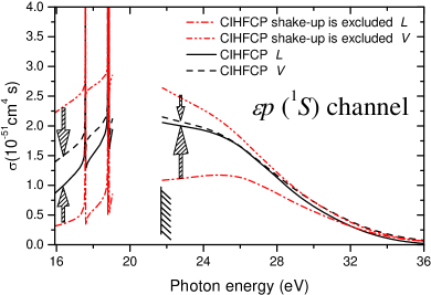
Figure 6: Partial G2PICS for the transition to the $3p^{5}\varepsilon p(^{1}S)$ channel, computed in length ($L$) and velocity ($V$) form for linearly polarized incoming radiation without (CIHFCP shake-up excluded) and with (CIHFCP) taking into account the shake-up correlation (IV). The two-photon $3p^{4}(^{3}P_{2})$ ionization threshold is indicated by the hatched line.

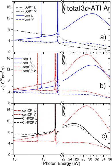
Figure 7: The computed total $3p$ shell G2PICS in length ($L$) and velocity ($V$) form for linearly polarized incoming radiation. (a) LOPT approach and considering all the correlations (I)-(VI) (corr); (b) polarization of the atomic core by the photoelectron (corrCP) is included in addition to a); (c) higher-order PT correlations (CIHFCP) are included in addition to b). The two-photon $3p^{4}(^{3}P_{2})$ ionization threshold is indicated by the hatched line.

Concluding this section we demonstrate the effect of a successive inclusion of different correlations in the calculated total $3p$ shell G2PICS in Fig. 7. In Fig. 7a, we compare the G2PICS computed in LOPT approximation with the cross sections obtained with taking into account correlations (II-VI). The drastic change of $\sigma(\omega)$ is obvious: a resonance structure appears below the two-photon $3p^{4}$ threshold and a considerable enhancement of the above-threshold cross section together with a change of the shape of $\sigma(\omega)$ from monotonic decrease to curve with a broad maximum occurs. Those changes are mainly due to the electron-scattering correlation (VI), i.e a $(3p\dashrightarrow\varepsilon d)^{2}$ absorption of two exciting photons at the giant resonance with a subsequent Auger type interaction $\varepsilon d\varepsilon d-3p\varepsilon f$. This mechanism should also influence the two-photon ATI of Xe in the range of its giant $4d\dashrightarrow\varepsilon f$ resonance. An experimental proof by determining the two-photon G2PICS in Ar or Xe close to their respective $3p^{4}$ and $4d^{8}$ thresholds would be highly desirable.

In Fig. 7b, the influence of the polarization of the atomic core by the photoelectron on the computed total cross section is presented. It results in a shift of the maximum of $\sigma(\omega)$ to lower photon energies and makes the humped curve more vivid. At the two-photon $3p^{4}(^{3}P_{2})$ threshold the G2PICS increases by $\sim 33\%$.

In Fig. 7c, the influence of the intrashell correlation on the dominating process (VI) and the effect of the correlational decrease of the Coulomb interaction on the transitions (II)-(VI) is shown. These higher-order PT corrections bring the cross sections computed in length and velocity form in the considered photon-energy regions together.

IV Angular distribution of photoelectrons

The expression for the differential G2PICS is as follows

$$\frac{d\sigma_{q}(\omega)}{d\Omega}=\frac{\sigma_{q}(\omega)}{4\pi}\\ \times\left[1+\beta_{2}^{q}(\omega)P_{2}(\cos\theta)+\beta_{4}^{q}(\omega)P_{4}(\cos\theta)\right],$$ (33)

where $\beta_{\lambda}^{q}$ are angular distribution parameters for photoelectrons, $P_{\lambda}$ are Legendre polynomials, $\theta$ is the angle between the momentum of the photoelectron and the electric field vectors for linearly polarized incident radiation ($q$ = 0) or between the momentum of photoelectron and the direction of propagation vectors of circularly polarized incoming radiation ($q=\pm 1$). The photoelectron angular distribution parameters $\beta_{\lambda}^{q}$ are expressed via the transition amplitudes $T_{q,\omega}(L,\ell)$ discussed above. The corresponding expressions and numerical coefficients are reported in petrov16 .

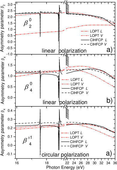
Figure 8: Angular-distribution parameters $\beta^{q}_{\lambda}$ for photoelectrons computed for the two-photon 3$p$ ATI of Ar in length ($L$) and velocity ($V$) form in LOPT approximation and with taking into account all the considered correlations (CIHFCP). The two-photon $3p^{4}(^{3}P_{2})$ ionization threshold is indicated by the hatched line.

The results of the present calculation are depicted in Figs. 8a,b,c for the $\beta_{2}^{0}$, $\beta_{4}^{0}$, and $\beta_{4}^{\pm 1}$ parameters, respectively. The $\beta_{2}^{0}$ and $\beta_{4}^{0}$ parameters describe the case of linearly polarized incoming radiation and $\beta_{4}^{\pm 1}$ is related to circularly polarized photons. The $\beta_{2}^{\pm 1}$ parameter is not presented in Fig. 8 because it is determined by the connection with $\beta_{4}^{\pm 1}$ via $\beta_{2}^{\pm 1}=-1-\beta_{4}^{\pm 1}$ petrov16 . In all cases taking into account many-electron correlations improves the agreement between length and velocity results.

The comparison between $\beta(\omega)$ computed in the LOPT approximation and with taking into account all the considered correlations exhibits a considerable change in $\beta(\omega)$ dependencies in the range where the doubly-excited resonances are situated. The influence of many-electron correlations on $\beta(\omega)$ at $\omega\gtrsim 22$ eV is less pronounced than in the G2PICS case. To a large extent this fact is connected with the prevalence of the $3p^{5}\varepsilon f$ channel in the two-photon photoionization of Ar due to the influence of the $3p\dashrightarrow\varepsilon d$ giant resonance.

V Conclusions

In the present work, the two-photon ionization of the 3$p$ shell of Ar in the above-threshold ionization (ATI) region was studied theoretically. For this purpose, we extended a noniterative correlation function (CF) technique developed earlier petrov16 to the case when both the CF and the final-state function are of continuum-type. An adequate accuracy of present calculations supported by good agreement between the results obtained in length and velocity form of dipole transition operator.

The many-electron correlation which can be treated as the $(3p\dashrightarrow\varepsilon d)^{2}$ absorption of the two exciting photons at giant resonance play a decisive role in two-photon ionization of Ar near the $3p^{4}$ threshold. Taking into account this correlation results in (i) an increase of the computed G2PICS by approximately three times and (ii) the appearance of resonance profiles in the energy range of the doubly-excited $3p^{4}n^{\prime}\ell^{\prime}n^{\prime\prime}\ell^{\prime\prime}$ states ($15.76<\omega<21.69$ eV).

Taking into account all remaining single and double electron excitations in computing the transition amplitudes results in better agreement between G2PICS-$L$ and G2PICS-$V$. Nevertheless, a 3 time difference between them in some partial photoionization channels still remains. This difference was removed after taking into account higher-order PT corrections. These corrections were included by: (i) the polarization of the atomic core by the photoelectron, realized by incorporation of an ab initio polarization potential in the Hamiltonian; (ii) the effective correlational decrease of the Coulomb interaction, taken into account by computing respective reduction coefficients; (iii) the intrashell correlations, taken into account via a technique described in amusia75 . Good agreement between length and velocity results for angular distribution parameters was also obtained after inclusion of the described above many-electron correlations.

Finally, our ab initio computation clarified that the two-photon above-threshold $3p$ ionization of Ar near the $3p^{4}$ threshold is almost entirely a collective-electron process. An experiment to benchmark the present calculation is desirable.

- (1) W. Ackermann, G. Asova, V. Ayvazyan, and A. Azima, Nat. Photonics 1, 336 (2007).
- (2) T. Shintake, H. Tanaka, T. Hara, and T. Tanaka, Nat. Photonics 2, 555 (2008).
- (3) P. Emma, R. Akre, J. Arthur, and R. Bionta, Nat. Photonics 4, 641 (2010).
- (4) T. Ishikawa, H. Aoyagi, T. Asaka, and Y. Asano, Nat. Photonics 6, 540 (2012).
- (5) H.-S. Kang, C.-K. Min, and H. Heo, Nat. Photonics 11, 708 (2017).
- (6) M. S. Pindzola and H. P. Kelly, Phys. Rev. A 11, 1543 (1975).
- (7) A. F. Starace and T.-F. Jiang, Phys. Rev. A 36, 1705 (1987).
- (8) A. L’Huillier and G. Wendin, Phys. Rev. A 36, 4747 (1987).
- (9) C. Pan, B. Gao, and A. F. Starace, Phys. Rev. A 41, 6271 (1990).
- (10) I. D. Petrov, B. M. Lagutin, V. L. Sukhorukov, A. Knie, and A. Ehresmann, Phys. Rev. A 93, 033408 (2016).
- (11) B. M. Lagutin, I. D. Petrov, V. L. Sukhorukov, P. V. Demekhin, A. Knie, and A. Ehresmann, Phys. Rev. A 95, 063414 (2017).
- (12) L.-W. Pi and A. F. Starace, Phys. Rev. A 82, 053414 (2010).
- (13) F. Herman and S. Skillman, Atomic Structure Calculations, N.J., Prentice-Hall, Englewood Cliffs, 1963.
- (14) F. Robicheaux and B. Gao, Phys. Rev. A 47, 2904 (1993).
- (15) A. R. Curtis, Corpuscles and Radiation in Matter, volume 11 of Royal Society Mathematical Tables, chapter Coulomb Wave Functions, pp. XXXV+209, (Cambridge, Univ.Press), 1964.
- (16) M. Aymar and M. Crance, J. Phys. B: At. Mol. Phys. 13, L287 (1980).
- (17) B. Gao and A. F. Starace, Comput. Phys. 1, 70 (1987).
- (18) T. Åberg and G. Howat, Corpuscles and Radiation in Matter, volume 31 of Enciclopedia of Physics, chapter Theory of the Auger effect, pp. 469–619, (Berlin: Springer), 1982.
- (19) A. Burgess, Proc. Phys. Soc. 81, 442 (1963).
- (20) A. Kramida, Y. Ralchenko, J. Reader, and NIST ASD Team, NIST Atomic Spectra Database (version 5.2)[Online], National Institute of Standards and Technology, Gaithersburg, MD, 2014, DOI:10.18434/T4W30F.
- (21) V. Sukhorukov, B. Lagutin, H. Schmoranzer, I. Petrov, and K.-H. Schartner, Phys. Lett. A 169, 445 (1992).
- (22) V. L. Sukhorukov, B. M. Lagutin, I. D. Petrov, S. V. Lavrentiev, H. Schmoranzer, and K. H. Schartner, J. Electron Spectrosc. Relat. Phenom. 68, 255 (1994).
- (23) S. Kammer, K.-H. Schartner, S. Mickat, R. Schill, A. Ehresmann, L. Werner, S. Klumpp, H. Schmoranzer, I. D. Petrov, P. V. Demekhin, and V. L. Sukhorukov, J. Phys. B: At. Mol. Opt. Phys. 39, 2757 (2006).
- (24) M. Amusia and N. Cherepkov, Many-electron correlations in scattering processes, volume 5 of Case Studies in Atomic Physics, pp. 49–179, North-Holland, Amsterdam, 1975.
- (25) I. D. Petrov, V. L. Sukhorukov, and H. Hotop, J. Phys. B: At. Mol. Opt. Phys. 32, 973 (1999).
- (26) K. Jorgensen, N. Andersen, and J. O. Olsen, J. Phys. B: At. Mol. Phys. 11, 3951 (1978).