Online Risk-Averse Submodular Maximization

Abstract

We present a polynomial-time online algorithm for maximizing the conditional value at risk (CVaR) of a monotone stochastic submodular function. Given $T$ i.i.d. samples from an underlying distribution arriving online, our algorithm produces a sequence of solutions that converges to a ($1-1/e$)-approximate solution with a convergence rate of $O(T^{-1/4})$ for monotone continuous DR-submodular functions. Compared with previous offline algorithms, which require $\Omega(T)$ space, our online algorithm only requires $O(\sqrt{T})$ space. We extend our online algorithm to portfolio optimization for monotone submodular set functions under a matroid constraint. Experiments conducted on real-world datasets demonstrate that our algorithm can rapidly achieve CVaRs that are comparable to those obtained by existing offline algorithms.

1 Introduction

Submodular function maximization is a ubiquitous problem naturally arising in broad areas such as machine learning, social network analysis, economics, combinatorial optimization, and decision-making (Krause and Golovin, 2014; Buchbinder and Feldman, 2018). Submodular maximization in these applications is stochastic in nature, i.e., the input data could be a sequence of samples drawn from some underlying distribution, or there could be some uncertainty in the environment. In this paper, we consider nonnegative monotone continuous DR-submodular (Bian et al., 2017) functions $F({\boldsymbol{x}};z)$ parameterized by a random variable $z$ drawn from some distribution $\mathcal{D}$. The simplest approach for such stochastic submodular objectives is to maximize the expectation $\operatorname*{\mathbf{E}}_{z\sim\mathcal{D}}[F({\boldsymbol{x}};z)]$, which has been extensively studied (Karimi et al., 2017; Hassani et al., 2017; Mokhtari et al., 2018; Karbasi et al., 2019).

However, in real-world decision-making tasks in finance, robotics, and medicine, we sometimes must be risk-averse: We want to minimize the risk of suffering a considerably small gain rather than simply maximizing the expected gain (Mansini et al., 2007; Yau et al., 2011; Tamar et al., 2015). In medical applications, for example, we must avoid catastrophic events such as patient fatalities. In finance and robotics, all progress ceases when poor decisions cause bankruptcies or irreversible damage to robots.

Conditional value at risk (CVaR) is a popular objective for such risk-averse domains (Rockafellar et al., 2000; Krokhmal et al., 2002). Formally, given a parameter $\alpha\in[0,1]$, the CVaR of a feasible solution ${\boldsymbol{x}}\in\mathbb{R}^{n}$ is defined as

$$\operatorname{CVaR}_{\alpha,\mathcal{D}}({\boldsymbol{x}})=\operatorname*{\mathbf{E}}_{z\sim\mathcal{D}}[F({\boldsymbol{x}};z)\mid F({\boldsymbol{x}};z)\leq\operatorname{VaR}_{\alpha,\mathcal{D}}({\boldsymbol{x}})],$$

where $\operatorname{VaR}_{\alpha,\mathcal{D}}(X)$ is the $\alpha$-quantile of the random variable $F({\boldsymbol{x}};z)$, i.e.,

$$\operatorname{VaR}_{\alpha,\mathcal{D}}(X)=\sup\left\{\tau\in\mathbb{R}:\Pr_{z\sim\mathcal{D}}(F({\boldsymbol{x}};z)\leq\tau)\leq\alpha\right\}.$$

Note that when $\alpha=1$, the CVaR is simply the expected value of $F({\boldsymbol{x}};z)$. Since $\alpha$ is typically set to be $0.10$ or $0.05$ in practice, we assume that $\alpha$ is a fixed constant throughout this paper. When $\alpha$ is clear from the context, we omit it from the notations. CVaR can also be characterized by a variational formula:

$$\operatorname{CVaR}_{\mathcal{D}}({\boldsymbol{x}})=\max_{\tau\in[0,1]}\tau-\frac{1}{\alpha}\operatorname*{\mathbf{E}}_{z\sim\mathcal{D}}{[\tau-F({\boldsymbol{x}};z)]}_{+},$$

where ${[\cdot]}_{+}=\max\{\cdot,0\}$ (Rockafellar et al., 2000).

Maehara (2015) initiated the study of maximizing the CVaR of stochastic submodular set functions. It was shown that the CVaR of a stochastic submodular set function is not necessarily submodular, and that it is impossible to compute a single set that attains any multiplicative approximation to the optimal CVaR. Ohsaka and Yoshida (2017) introduced a relaxed problem of finding a portfolio over sets rather than a single set, and devised the first CVaR maximization algorithm with an approximation guarantee for the influence maximization problem (Kempe et al., 2003), a prominent example of discrete submodular maximization. Wilder (2018) further considered this approach and devised an algorithm called RASCAL for maximizing the CVaR of continuous DR-submodular functions subject to a down-closed convex set.

The algorithms mentioned above are offline (batch) methods, i.e., a set of samples drawn from the underlying distribution $\mathcal{D}$ is given as the input. However, because the number of samples needed to accurately represent $\mathcal{D}$ can be exceedingly large, it is often inefficient or even impossible to store all the samples in memory. Further, when a new sample is observed, these offline algorithms must be rerun from scratch.

In the machine learning community, online methods, which can efficiently handle large volumes of data, have been extensively studied (Hazan, 2016). Online methods read data in a streaming fashion, and update the current solution using a few data elements stored in memory. Further, online methods can update a solution at a low computational cost.

1.1 Our contributions

In this work, we propose online algorithms for maximizing the CVaR of stochastic submodular objectives in continuous and discrete settings.

Continuous setting

Let $z_{1},\dots,z_{T}$ be i.i.d. samples drawn from $\mathcal{D}$ arriving sequentially and $K\subseteq\mathbb{R}^{n}$ be a down-closed convex set. Our main result is a polynomial-time online algorithm, StochasticRASCAL, that finds ${\boldsymbol{x}}\in K$ such that

$$\operatorname*{\mathbf{E}}[\operatorname{CVaR}_{\mathcal{D}}({\boldsymbol{x}})]\geq\left(1-\frac{1}{e}\right)\operatorname{CVaR}_{\mathcal{D}}({\boldsymbol{x}}^{*})-O(T^{-1/4}),$$

for any ${\boldsymbol{x}}^{*}\in K$, where the expectation is taken over $z_{1},\dots,z_{T}$ and the randomness of the algorithm. StochasticRASCAL only stores $O(\sqrt{T})$ data in memory, drawing a contrast to RASCAL, which store all $T$ data points. Note that the approximation ratio of $1-1/e$ is optimal for any algorithm that performs polynomially many function value queries even if $\alpha=1$ (Vondrák, 2013). We also conduct several experiments on real-world datasets to show the practical efficiency of our algorithm. We demonstrate that our algorithm rapidly achieves CVaR comparable to that obtained by known offline methods.

Discrete setting

As an application of the above algorithm, we devise an online algorithm to create a portfolio that maximizes the CVaR of a discrete submodular function subject to a matroid constraint. Let $f(X;z):2^{V}\to[0,1]$ be a monotone stochastic submodular set function on a ground set $V$ and $\mathcal{I}\subseteq 2^{V}$ be a matroid. The goal is to find a portfolio $\mathcal{P}$ of feasible sets in $\mathcal{I}$ that maximizes

$$\operatorname{CVaR}_{\mathcal{D}}(\mathcal{P})=\max_{\tau\in[0,1]}\tau-\frac{1}{\alpha}\operatorname*{\mathbf{E}}_{z\sim\mathcal{D}}[\tau-\operatorname*{\mathbf{E}}_{X\sim\mathcal{P}}f(X;z)]_{+},$$

given i.i.d. samples from $\mathcal{D}$. We show that this problem can be reduced to online CVaR maximization of continuous DR-submodular functions on a matroid polytope, and devise a polynomial-time online approximation algorithm for creating a portfolio $\mathcal{P}$ such that

$$\operatorname*{\mathbf{E}}[\operatorname{CVaR}_{\mathcal{D}}(\mathcal{P})]\geq\left(1-\frac{1}{e}\right)\operatorname{CVaR}_{\mathcal{D}}(\mathcal{P}^{*})-O(T^{-1/10})$$

for any portfolio $\mathcal{P}^{*}$ over feasible sets. Note that this algorithm is the first online algorithm that converges to a $(1-1/e)$-approximation portfolio in the discrete setting, which generalizes the known offline algorithm (Wilder, 2018) to the i.i.d. setting.

1.2 Our techniques

To analyze our online algorithms, we introduce a novel adversarial online learning problem, which we call adversarial online submodular CVaR learning. This online learning problem is described as follows. For $t=1,\dots,T$, the learner chooses ${\boldsymbol{x}}_{t}\in K$ and $\tau_{t}\in[0,1]$ possibly in a randomized manner. After ${\boldsymbol{x}}_{t}$ and $\tau_{t}$ are chosen, the adversary reveals a monotone continuous DR-submodular function $F_{t}:K\to[0,1]$ to the learner. The goal of the learner is to minimize the approximate regret

$$\operatorname{regret}_{1-1/e}(T)=\left(1-\frac{1}{e}\right)\sum_{t=1}^{T}H_{t}({\boldsymbol{x}}^{*},\tau^{*})-\sum_{t=1}^{T}H_{t}({\boldsymbol{x}}_{t},\tau_{t})$$

for arbitrary ${\boldsymbol{x}}^{*}\in K$ and $\tau^{*}\in[0,1]$, where the function $H_{t}$ is given by

$$H_{t}({\boldsymbol{x}},\tau)=\tau-\frac{1}{\alpha}{[\tau-F_{t}({\boldsymbol{x}})]}_{+}.$$

We devise an efficient algorithm that achieves $O(T^{3/4})$ approximate regret in expectation. Further, we show that, given an online algorithm with a sublinear approximate regret, we can construct an online algorithm that achieves a $(1-1/e)$-approximation to CVaR maximization, whose convergence rate is $\operatorname*{\mathbf{E}}[\operatorname{regret}_{1-1/e}(T)]/T$. Combining these results, we obtain an online $(1-1/e)$-approximation algorithm for CVaR maximization with a convergence rate of $O(T^{-1/4})$.

We remark that adversarial online submodular CVaR learning may be of interest in its own right: Although the objective function $H_{t}$ is neither monotone nor continuous DR-submodular in general, we can design an online algorithm with a sublinear ($1-1/e$)-regret by exploiting the underlying structure of $H_{t}$. As per our knowledge, an online algorithm for non-monotone and non-DR-submodular maximization does not exist in the literature.

1.3 Related work

Several studies focused on CVaR optimization in the adversarial online settings and i.i.d. settings. Tamar et al. (2015) studied CVaR optimization over i.i.d. samples and analyzed stochastic gradient descent under the strong assumption that CVaR is continuously differentiable. Recently, Cardoso and Xu (2019) introduced the concept of the CVaR regret for convex loss functions and provided online algorithms for minimizing the CVaR regret under bandit feedback.

Online and stochastic optimization of submodular maximization have been extensively studied in Streeter and Golovin (2008); Streeter et al. (2009); Golovin et al. (2014); Karimi et al. (2017); Hassani et al. (2017); Mokhtari et al. (2018); Chen et al. (2018); Roughgarden and Wang (2018); Soma (2019); Karbasi et al. (2019); Zhang et al. (2019). These studies optimize either the approximate regret or the expectation and do not consider CVaR.

Another line of related work is robust submodular maximization (Krause et al., 2008; Chen et al., 2017; Anari et al., 2019). In robust submodular maximization, we maximize the minimum of $N$ submodular functions, i.e., $\min_{i=1}^{N}f_{i}(X)$. Robust submodular maximization is the limit of CVaR maximization, where $\mathcal{D}$ is the uniform distribution over $N$ values and $\alpha\to 0$. Recently, Staib et al. (2019) proposed distributionally robust submodular optimization, which maximizes $\min_{\mathcal{D}\in P}\operatorname*{\mathbf{E}}_{z\sim\mathcal{D}}f(X;z)$ for an uncertainty set $P$ of distributions. It is known that CVaR can be formulated in the distributionally robust framework (Shapiro et al., 2014). However, the algorithms proposed by Staib et al. (2019) require that $P$ is a subset of the $N$-dimensional probability simplex; moreover, their time complexity depends on $N$. Our algorithms work even if $N$ is infinite.

1.4 Organization of this paper

This paper is organized as follows. Section 2 introduces the background of submodular optimization. Sections 3 and 4 describe our algorithms for continuous and discrete setting, respectively. Section 5 present experimental results using real-world dataset. The omitted analysis and the details of adversarial setting can be found in Appendix.

2 Preliminaries

Throughout the paper, $V$ denotes the ground set and $n$ denotes the size of the ground set. For a set function $f:2^{V}\to\mathbb{R}$, the multilinear extension $F:[0,1]^{V}\to\mathbb{R}$ is defined as $F({\boldsymbol{x}})=\sum_{S\subseteq V}f(S)\prod_{i\in S}x_{i}\prod_{i\notin S}(1-x_{i})$. For a matroid on $V$, the base polytope is the convex hull of bases of the matroid. It is well-known that the linear optimization on a base polytope can be solved by the greedy algorithm (Fujishige, 2005).

We denote the Euclidean norm and inner product by $\lVert\cdot\rVert$ and $\langle\cdot,\cdot\rangle$, respectively. The $\ell^{p}$ norm ($1\leq p\leq\infty$) is denoted by $\lVert\cdot\rVert_{p}$. The Euclidean projection of ${\boldsymbol{x}}$ onto a set $K$ is denoted by $\operatorname{proj}_{K}({\boldsymbol{x}})$. A convex set $K\subseteq\mathbb{R}_{\geq 0}^{n}$ is said to be down-closed if ${\boldsymbol{y}}\in K$ and $\mathbf{0}\leq{\boldsymbol{x}}\leq{\boldsymbol{y}}$ imply ${\boldsymbol{x}}\in K$. A function $f:\mathbb{R}^{n}\to\mathbb{R}$ is said to be $L$-Lipschitz (continuous) for $L>0$ if $\lvert f({\boldsymbol{x}})-f({\boldsymbol{y}})\rvert\leq L\lVert{\boldsymbol{x}}-{\boldsymbol{y}}\rVert$ for all ${\boldsymbol{x}},{\boldsymbol{y}}$. We say that $f$ is $\beta$-smooth for $\beta>0$ if $f$ is continuously differentiable and $\lVert\nabla f({\boldsymbol{x}})-\nabla f({\boldsymbol{y}})\rVert\leq\beta\lVert{\boldsymbol{x}}-{\boldsymbol{y}}\rVert$. A smooth function $F:\mathbb{R}^{n}\to\mathbb{R}$ is said to be continuous DR-submodular (Bian et al., 2017) if $\frac{\partial^{2}F}{\partial x_{i}\partial x_{j}}\leq 0$ for all $i,j$. The multilinear extension of a submodular function is known to be DR-submodular (Calinescu et al., 2011). The continuous DR-submodularity implies up-concavity: For a continuous DR-submodular function $F$, ${\boldsymbol{x}}\in\mathbb{R}^{n}$, and ${\boldsymbol{d}}\geq\mathbf{0}$, the univariate function $t\mapsto F({\boldsymbol{x}}+t{\boldsymbol{d}})$ is concave.

The uniform distribution of a set $K$ is denoted by $\mathrm{Unif}(K)$. The standard normal distribution is denoted by $N(\mathbf{0},I)$.

3 CVaR Maximization of Continuous DR-submodular Functions

We present our online algorithm for CVaR maximization via i.i.d. samples. Let $F_{t}:\mathbb{R}^{n}\to[0,1]$ be the monotone continuous DR-submodular function corresponding to the $t$-th sample $z_{t}$, i.e.,

$$F_{t}({\boldsymbol{x}})=F({\boldsymbol{x}};z_{t})$$

for $t=1,\dots,T$. Similarly, define an auxiliary function $H_{t}$ with respect to $z_{t}$ by

$$H_{t}({\boldsymbol{x}},\tau)=\tau-\frac{1}{\alpha}{[\tau-F_{t}({\boldsymbol{x}})]}_{+}=\tau-\frac{1}{\alpha}{[\tau-F({\boldsymbol{x}};z_{t})]}_{+}.$$

for $t=1,\dots,T$. Let $K\subseteq\mathbb{R}_{\geq 0}^{n}$ be a down-closed convex set. Formally, we make the following very mild assumptions on $F_{t}$ and $K$.

Assumption 1.

x

• For all $t$, $F_{t}$ is $L$-Lipschitz and $\beta$-smooth, and $\lVert\nabla F_{t}\rVert\leq G$.

• The diameter of $K$ is bounded by $D$.

• We are given a linear optimization oracle over $K$.

When the underlying norm is the $\ell^{p}$-norm with $p\neq 2$, we write $G_{p}$ to emphasize it. For example, if $F_{t}$ is the multilinear extension of a submodular set function $f_{t}:2^{V}\to[0,1]$ and $K$ is the base polytope of a rank-$k$ matroid, we have $L=\beta=O(n)$, $G_{\infty}=1$, $D=O(\sqrt{k})$.

Our algorithm borrows some ideas from an algorithm called RASCAL (Wilder, 2018). First, we define a smoothed auxiliary function $\tilde{H}_{t}:{[0,1]}^{V}\times[0,1]\to[0,1]$ as

$$\tilde{H}_{t}({\boldsymbol{x}},\tau)=\frac{1}{u}\int_{0}^{u}\left(\tau+\xi-\frac{1}{\alpha}{[\tau+\xi-F_{t}({\boldsymbol{x}})]}_{+}\right)d\xi,$$

where $u>0$ is a smoothing parameter specified later. This smoothing guarantees that $\tilde{H}_{t}$ is differentiable for all ${\boldsymbol{x}}$ and has Lipschitz continuous gradients.

Lemma 2 (Lemma 6 of Wilder (2018)).

x

1. $\lvert H_{t}({\boldsymbol{x}},\tau)-\tilde{H}_{t}({\boldsymbol{x}},\tau)\rvert\leq\frac{u(1+1/\alpha)}{2}$ for all ${\boldsymbol{x}}$ and $\tau$.

2. If $F_{t}$ is $L$-Lipschitz and $\beta$-smooth, and $\lVert\nabla F_{t}\rVert\leq G$, then $\nabla_{\boldsymbol{x}}\tilde{H}_{t}$ is $\frac{1}{\alpha}(\beta+\frac{LG}{u})$-Lipschitz.

Lemma 3 (Wilder (2018)).

The function $\max_{\tau}\tilde{H}_{t}(\cdot,\tau)$ is monotone and up-concave.

3.1 StochasticRASCAL

We now formally describe our algorithm, StochasticRASCAL. We note that RASCAL runs the Frank-Wolfe algorithm on a function $\max_{\tau}\sum_{t=1}^{T}\tilde{H}_{t}(\cdot,\tau)$. Owing to the up-concavity and smoothness properties of this function, one can obtain $(1-1/e)$-approximation. However, in our online setting, we cannot evaluate this function because $\tilde{H}_{t}$ will be revealed online, and hence we cannot simply run RASCAL.

To overcome the issue above, first we split the $T$ samples into mini-batches of length $B$, which we specify later. The key idea is to use the following objective function

$$\bar{H}_{b}({\boldsymbol{x}})=\max_{\tau}\frac{1}{B}\sum_{t=(b-1)B+1}^{bB}\tilde{H}_{t}({\boldsymbol{x}},\tau)$$

for each $b$-th mini-batch ($b=1,\dots,T/B$). We can see that $\bar{H}_{b}({\boldsymbol{x}})$ is monotone, up-concave, and can be evaluated only using samples in the $b$-th mini-batch. Then, we run a perturbed version of Frank-Wolfe algorithm (Golovin et al., 2014; Bian et al., 2017) on $\bar{H}_{b}$. More formally, we first initialize ${\boldsymbol{x}}_{b+1}^{0}=\mathbf{0}$ and for each $s=0,\delta,2\delta,\dots,1-\delta$, we perform the update

$${\boldsymbol{x}}_{b}^{s+\delta}\leftarrow{\boldsymbol{x}}_{b}^{s}+\delta{\boldsymbol{d}}_{b}^{s}$$

where $\delta$ is the step size, ${\boldsymbol{d}}_{b}^{s}$ is a solution to a perturbed linear optimization problem on $K$:

$${\boldsymbol{d}}_{b}^{s}\in\operatorname*{argmax}_{{\boldsymbol{d}}\in K}\left\langle\lambda\sum_{b^{\prime}=1}^{b}{\nabla\bar{H}_{b^{\prime}}}({\boldsymbol{x}}_{b^{\prime}}^{s})+{\boldsymbol{r}}_{b}^{s},{\boldsymbol{d}}\right\rangle.$$

Here, ${\boldsymbol{r}}_{b}^{s}\sim\mathcal{D}_{\mathrm{FPL}}$ is a perturbation vector. This perturbation trick aims to stabilize the algorithm so that we can maximize the true objective $\max_{\tau}\sum_{t=1}^{T}\tilde{H}_{t}(\cdot,\tau)$ using only mini-batch objectives.

In each iteration of continuous greedy, we need the gradients $\nabla\bar{H}_{b}({\boldsymbol{x}}_{b}^{s})$, which in turn requires us to compute $\operatorname*{argmax}_{\tau}\frac{1}{B}\sum_{t=(b-1)B+1}^{bB}\tilde{H}_{t}({\boldsymbol{x}}_{b}^{s},\tau)$. These gradients and the optimal $\tau$ can be computed by SmoothGrad and SmoothTau subroutines, respectively, which were proposed in Wilder (2018); See Algorithms 2 and 3.

Let us write ${\boldsymbol{x}}_{b}:={\boldsymbol{x}}_{b}^{1}$ for $b=1,\dots,T/B$. The final output of StochasticRASCAL is ${\boldsymbol{x}}_{b^{\prime}}$ for a random index $b^{\prime}$ chosen uniformly at random from $\{1,2,\dots,T/B\}$. The pseudocode of StochasticRASCAL is presented in Algorithm 1.

Algorithm 1 StochasticRASCAL

0:  learning rates $\lambda>0$, step size $\delta>0$, perturbation distribution $\mathcal{D}_{\mathrm{FPL}}$, smoothing parameter $u>0$, and mini-batch size $B>0$

1:  Initialize ${\boldsymbol{x}}_{1}\in K$ arbitrary.

2:  for $b=1,\dots,T/B$ do

3:     Observe samples $z_{(b-1)B+1},\dots,z_{bB}$ and store them in mini-batch $\mathcal{Z}_{b}$.

4:     /* continuous greedy */

5:     Let ${\boldsymbol{x}}_{b}^{0}\leftarrow\mathbf{0}$.

6:     for $s=0,\delta,2\delta,\dots,1-\delta$ do

7:        $\tau:=\textsc{SmoothTau}({\boldsymbol{x}}_{b}^{s},u,\mathcal{Z}_{b})$

8:        ${\boldsymbol{g}}_{b}^{s}:=\textsc{SmoothGrad}({\boldsymbol{x}}_{b}^{s},\tau,u,\mathcal{Z}_{b})$.

9:        Find a vertex ${\boldsymbol{d}}_{b+1}^{s}$ of $K$ that maximizes $\left\langle\lambda\sum_{b^{\prime}=1}^{b}{\boldsymbol{g}}_{b^{\prime}}^{s}+{\boldsymbol{r}}_{b}^{s},{\boldsymbol{d}}\right\rangle$ for ${\boldsymbol{d}}\in K$, where ${\boldsymbol{r}}_{b}^{s}\sim\mathcal{D}_{\mathrm{FPL}}$. // FPL

10:        ${\boldsymbol{x}}_{b}^{s+\delta}\leftarrow{\boldsymbol{x}}_{b}^{s}+\delta{\boldsymbol{d}}_{b}^{s}$

11:     end for

12:     Let ${\boldsymbol{x}}_{b}={\boldsymbol{x}}_{b}^{1}$.

13:  end for

14:  return  ${\boldsymbol{x}}_{b^{\prime}}$ for $b^{\prime}$ chosen from $\{1,2,\dots,T/B\}$ uniformly at random.

Algorithm 2 SmoothGrad$({\boldsymbol{x}},\tau,u,\mathcal{Z})$

0:  ${\boldsymbol{x}}$, $\tau$, $u$, and mini-batch $\mathcal{Z}$

1:  $I_{z}(\tau):=\max\{\min\{\frac{F({\boldsymbol{x}};z)-\tau}{u},1\}$ for $z\in\mathcal{Z}$.

2:  return  $\sum_{z\in\mathcal{Z}}I_{z}(\tau)\nabla_{\boldsymbol{x}}F({\boldsymbol{x}},z)$

Algorithm 3 SmoothTau$({\boldsymbol{x}},u,\mathcal{Z})$

0:  ${\boldsymbol{x}}$, $u$, and mini-batch $\mathcal{Z}$

1:  $\mathcal{B}:=\{F({\boldsymbol{x}};z)\mid z\in\mathcal{Z}\}\cup\{F({\boldsymbol{x}};z)+u\mid z\in\mathcal{Z}\}$

2:  Sort $\mathcal{B}$ in ascending order, obtaining $\mathcal{B}=\{b_{1},\dots,b_{\lvert\mathcal{B}\rvert}\}$.

3:  $i^{*}:=\min\{i:\sum_{z\in\mathcal{Z}}I_{z}(b_{i})<\alpha\lvert\mathcal{Z}\rvert\}$

4:  $A:=\{z\in\mathcal{Z}:b_{i^{*}-1}<F({\boldsymbol{x}};z)<b_{i^{*}}\}$

5:  $C:=\{z\in\mathcal{Z}:F({\boldsymbol{x}};z)\leq b_{i^{*}-1}\}$

6:  return  the solution $\tau$ of the linear equation

$$\sum_{z\in\mathcal{Z}}\frac{F({\boldsymbol{x}};z)-\tau}{u}+\lvert C\rvert=\alpha\lvert\mathcal{Z}\rvert.$$

3.2 Convergence rate via regret bounds

Let us consider the convergence rate of StochasticRASCAL. The main challenge of the analysis is how to set the parameters used in the algorithm, i.e., learning rates $\lambda$, step size $\delta$, perturbation distribution $\mathcal{D}_{\mathrm{FPL}}$, smoothing parameter $u$, and mini-batch size $B$, to achieve the desired $O(T^{-1/4})$ convergence rate.

To this end, using tools from online convex optimization, we prove an approximate regret bound for a variant of StochasticRASCAL for adversarial online submodular CVaR learning (see Introduction for the definition).

Theorem 4 (informal).

There exists an efficient online algorithm for adversarial online CVaR learning with

$$\left(1-\frac{1}{e}\right)\sum_{t=1}^{T}H_{t}({\boldsymbol{x}}^{*},\tau^{*})-\operatorname*{\mathbf{E}}\left[\sum_{t=1}^{T}H_{t}({\boldsymbol{x}}_{t},\tau_{t})\right] =O(T^{3/4})$$

for an arbitrary ${\boldsymbol{x}}^{*}\in K$ and $\tau^{*}\in[0,1]$, where the big-O notation hides a factor polynomial in $\alpha,\beta,D,G$, and $n$.

We then show that the above regret bound can be used to show a convergence rate of StochasticRASCAL. The technical detail of the adversarial setting and the proof of the following theorem is deferred to Appendix.

Theorem 5.

Under Assumption 1, StochasticRASCAL outputs ${\boldsymbol{x}}\in K$ such that for any ${\boldsymbol{x}}^{*}\in K$,

$$\operatorname*{\mathbf{E}}[\operatorname{CVaR}_{\mathcal{D}}({\boldsymbol{x}})]$$

$$\geq\left(1-\frac{1}{e}\right)\operatorname{CVaR}_{\mathcal{D}}({\boldsymbol{x}}^{*})-O\left(\frac{\sqrt{C_{\alpha}GD}n^{1/8}}{\sqrt{\alpha}}\right)T^{-1/4},$$

where we set $B=\frac{\alpha C_{\alpha}\sqrt{T}}{DGn^{1/4}}$, $\delta=\frac{\alpha^{2}}{D^{2}\left((1+\alpha)GL\sqrt{T}+\alpha\beta T^{1/4}\right)}$, $\lambda=\frac{\alpha Dn^{1/4}\sqrt{B/T}}{G}$, $u=\frac{T^{-1/4}}{(1+1/\alpha)}$, and $\mathcal{D}_{\mathrm{FPL}}=\mathrm{Unif}({[0,1]}^{n})$, and $C_{\alpha}:=\max\{1,\frac{1}{\alpha}-1\}$. Further, if $K$ is an integral polytope contained in $\{{\boldsymbol{x}}\in{[0,1]}^{n}:\sum_{i}x_{i}=k\}$, then

$$\operatorname*{\mathbf{E}}[\operatorname{CVaR}_{\mathcal{D}}({\boldsymbol{x}})]$$

$$\geq\left(1-\frac{1}{e}\right)\operatorname{CVaR}_{\mathcal{D}}({\boldsymbol{x}}^{*})-O\left(\frac{\sqrt{C_{\alpha}G_{\infty}}k^{3/4}\log^{1/4}n}{\sqrt{\alpha}}\right)T^{-1/4}$$

for $B=\frac{\sqrt{2}C_{\alpha}\sqrt{T}\alpha}{2G_{\infty}k^{3/2}\sqrt{\log{\left(n\right)}}}$, $\delta=\frac{\alpha^{2}}{D^{2}\left((1+\alpha)GL\sqrt{T}+\alpha\beta T^{1/4}\right)}$, $\lambda=\sqrt{\frac{B}{Tk}}$, $u=\frac{T^{-1/4}}{(1+1/\alpha)}$, and $\mathcal{D}_{\mathrm{FPL}}=N(\mathbf{0},I)$.

To achieve $\operatorname*{\mathbf{E}}[\operatorname{CVaR}_{\mathcal{D}}({\boldsymbol{x}})]\geq\left(1-\frac{1}{e}\right)\operatorname{CVaR}_{\mathcal{D}}({\boldsymbol{x}}^{*})-\varepsilon$ for a desired error $\varepsilon>0$, StochasticRASCAL requires $O(\frac{D^{2}G^{2}\sqrt{n}}{\varepsilon^{4}})$ samples and $O(\frac{DGn^{1.25}}{\varepsilon^{2}})$ space, whereas RASCAL (Wilder, 2018) requires $O(\frac{n}{\varepsilon^{2}})$ samples and $O(\frac{n^{2}}{\varepsilon^{2}})$ space. Our algorithm runs in a smaller space when the parameters are of moderate size. For example, if $\beta=D=O(1)$ and $L=G=o(n^{1/4})$, the space complexity of StochasticRASCAL is better than that of RASCAL.

4 CVaR Maximization of Discrete Submodular Functions

We now present our online algorithm for a monotone submodular set function and a matroid constraint. Let $f_{t}:2^{V}\to[0,1]$ be a monotone submodular function corresponding to the $t$-th sample and $F_{t}$ be its multilinear extension for $t=1,\dots,T$.

The basic idea is to run StochasticRASCAL on the multilinear extensions $F_{t}$ and the matroid polytope $K$. However, we must address several technical obstacles. First, we must compare the output portfolio with the optimal portfolio; the error bound in the previous sections compared it with the optimal solution. To this end, we make multiple copies of variables so that we can approximate an optimal portfolio by a uniform distribution over a multiset of feasible solutions. More precisely, we define a continuous DR-submodular function $\bar{F}_{t}:K^{r}\to[0,1]$ by

$$\bar{F}_{t}({\boldsymbol{x}}^{1},\dots,{\boldsymbol{x}}^{r})=\frac{1}{r}\sum_{i=1}^{r}F_{t}({\boldsymbol{x}}^{i})$$

for some sufficiently large $r$. Then, we feed $\bar{F}_{1},\dots,\bar{F}_{T}$ to StochasticRASCAL. Suppose that we obtain $({\boldsymbol{x}}_{b}^{1},\dots,{\boldsymbol{x}}_{b}^{r})$ at Line 12 for each mini-batch $b=1,\dots,T/B$. Abusing the notation, let us denote $({\boldsymbol{x}}_{t}^{1},\dots,{\boldsymbol{x}}_{t}^{r}):=({\boldsymbol{x}}_{b}^{1},\dots,{\boldsymbol{x}}_{b}^{r})$ when the $t$-th sample is in the $b$-th mini-batch.

Next, we need to convert ${\boldsymbol{x}}_{t}^{1},\dots,{\boldsymbol{x}}_{t}^{r}$ to feasible sets without significantly deteriorating the values of the multilinear extensions. To this end, we independently apply randomized swap rounding (Chekuri et al., 2010) $q$ times to each ${\boldsymbol{x}}^{i}$ to obtain feasible sets $X_{t}^{i,1},\dots,X_{t}^{i,q}$. Note that randomized swap rounding is oblivious rounding and independent from $F_{t}$. We can show that $\frac{1}{q}\sum_{j=1}^{q}f_{t}(X_{t}^{i,j})$ is close to $F_{t}({\boldsymbol{x}}_{t}^{i})$ by using a concentration inequality. Finally, after $T$ rounds, we return the uniform portfolio over all $X_{t}^{i,q}$. The pseudocode is given in Algorithm 4. Carefully choosing $r$ and $q$, we obtain the following theorem.

Algorithm 4 Online algorithm for maximizing a monotone submodular set function subject to a matroid constraint.

1:  Run StochasticRASCAL for $\bar{F_{1}},\dots,\bar{F_{T}}$ and the matroid polytope $K$ and let $({\boldsymbol{x}}_{t}^{1},\dots,{\boldsymbol{x}}_{t}^{r})$ be the temporary solution at Line 12 in StochasticRASCAL for $t=1,\dots,T$.

2:  $X_{t}^{i,j}\leftarrow\textsc{RandomizedSwapRounding}({\boldsymbol{x}}_{t}^{i})$ for $t=1,\dots,T$, $i=1,\dots,r$, and $j=1,\dots,q$.

3:  return  Uniform portfolio $\bar{\mathcal{P}}$ over all $X_{t}^{i,j}$.

Theorem 6.

Algorithm 4 achieves

$$\operatorname*{\mathbf{E}}[\operatorname{CVaR}(\bar{\mathcal{P}})]$$

$$\geq\left(1-\frac{1}{e}\right)\operatorname{CVaR}_{\mathcal{D}}(\mathcal{P}^{*})-O(k^{3/4}\log^{1/4}(n)T^{-1/10})$$

for arbitrary portfolio $\mathcal{P}^{*}$, where we set $r=\tilde{O}(T^{1/5})$ and $q=\tilde{O}(T^{3/4})$ and the expectation is taken over $z_{1},\dots,z_{T}$ and the randomness of the algorithm.

5 Experiments

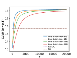
(a) NetScience

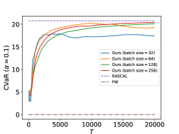
(b) EuroRoad

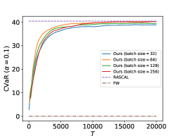
(c) BWSN

Figure 1: CVaR and the number of samples $T$

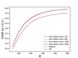
(a) NetScience

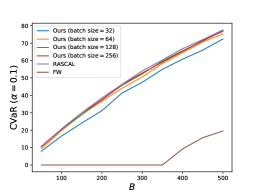
(b) EuroRoad

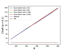
(c) BWSN

Figure 2: CVaR and budget $B$

In this section, we show our experimental results. In all the experiments, the parameter $\alpha$ of CVaR was set to $0.1$. The experiments were conducted on a Linux server with Intel Xeon Gold 6242 (2.8GHz) and 384GB of main memory.

Problem Description.

We conducted experiments on the sensor resource allocation problem, in which the goal is to rapidly detect a contagion spreading through a network using a limited budget (Bian et al., 2017; Leskovec et al., 2007; Soma and Yoshida, 2015).

Here, we follow the configuration of the experiments conducted in Wilder (2018). Let $G=(V,E)$ be a graph on $n$ vertices. A contagion starts at a random vertex and spreads over time according to some specific stochastic process. Let $z_{v}$ be the time at which the contagion reaches $v$, and let $z_{\max}=\max_{v\in V:z_{v}<\infty}z_{v}$. If $z_{v}=\infty$ for some vertex $v\in V$, that is, the contagion does not reach $v$, we reassign $z_{v}=z_{\max}$, as described in Wilder (2018).

The decision maker has a budget $B$ (e.g., energy) to spend on sensing resources. Let $x_{v}$ represent the amount of energy allocated to the sensor at a vertex $v$. When contagion reaches $v$ at time $z_{v}$, the sensor detects it with probability $1-{(1-p)}^{x_{v}}$, where $p\in[0,1]$ is the probability that detects the contagion per unit of energy. The objective $F$ on vectors ${\boldsymbol{x}}={(x_{v})}_{v\in V}$ and ${\boldsymbol{z}}={(z_{v})}_{v\in V}$ is the expected amount of detection time that is saved by the sensor placements:

$$F({\boldsymbol{x}};{\boldsymbol{z}})=z_{\max}-\sum_{i=1}^{n}z_{v_{i}}(1-{(1-p)}^{x_{v_{i}}})\prod_{j<i}{(1-p)}^{x_{v_{j}}},$$

where the vertices are ordered so that $z_{v_{1}}\leq z_{v_{2}}\leq\cdots\leq z_{v_{n}}$. It is known that the function $F$ is DR-submodular (Bian et al., 2017).

Datasets.

We consider two sensing models and generated three datasets. In all of them, the source vertex $s$ is chosen uniformly at random.

The first model is the continuous time independent cascade model (CTIC). In this model, each edge $uv\in E$ has propagation time $\rho_{uv}$ drawn from an exponential distribution with mean $\lambda$. The contagion starts at the source vertex $s$, i.e., $z_{s}=0$, and we iteratively set $z_{v}=\min_{u\in N(v)}z_{u}+\rho_{uv}$, where $N(v)$ is the set of neighbors of $v$. Note that $z_{v}$ is the first time that the contagion reaches $v$ from its neighbor. We generated datasets using two real-world networks: NetScience, a collaboration network of 1,461 network scientists, and EuroRoad, a network of 1,174 European cities and the roads between them. For both networks, we set $\lambda=5$ and $p=0.01$, and we generated 1,000 scenarios.

The second model, known as the Battle of Water Sensor Networks (BWSN) (Ostfeld and others, 2008), involves contamination detection in a water network. BWSM simulates the spread of contamination through a 126-vertex water network consisting of junctions, tanks, pumps, and the links between them, and the $z_{v}$ values are provided by a simulator. We set $p=0.001$ and generated 1,000 scenarios.

Methods.

We compared our method against two offline algorithms, RASCAL (Wilder, 2018) and the Frank–Wolfe (FW) algorithm (Bian et al., 2017). We note that the latter algorithm is designed to maximize the expectation of a DR-submodular function instead of its CVaR. We run those offline methods on the generated 1,000 scenarios for each dataset. As our method is an online algorithm, we run our method on 20,000 samples in an online manner, where each sample was uniformly drawn from the set of generated scenarios.

Results.

Figure 1 shows how the CVaR changes as $T$ increases. For each dataset, as long as the batch size is not excessively small, the CVaR attained by our method approaches to that attained by RASCAL. FW algorithm showed significantly lower performance because it is not designed to maximize CVaR.

Figure 2 shows how the CVaR changes as the budget $B$ increases. For our method, we plotted the CVaR after processing $10,000$ samples. We can again confirm that the CVaR attained by our method is close to that attained by RASCAL.

6 Conclusion

We devised StochasticRASCAL for maximizing CVaR of a monotone stochastic submodular function. We showed that StochasticRASCAL finds a ($1-1/e$)-approximate solution with a convergence rate of $O(T^{-1/4})$ for monotone continuous DR-submodular functions. We extended it to portfolio optimization for monotone submodular set functions under a matroid constraint. Experiments using CTIC and BWSN datasets demonstrated that our algorithm can rapidly achieve CVaRs that are comparable to RASCAL.

Appendix A Adversarial Setting

In this section, we present online algorithm for CVaR maximization in an adversarial environment.

A.1 Preliminaries on Online Convex Optimization

We use the framework called online convex optimization (OCO) extensively, and will briefly explain it below. For details, the reader is referred to a monograph [Hazan, 2016]. In OCO, the learner is given a compact convex set $K\subseteq\mathbb{R}^{n}$. For each round $t=1,\dots,T$, the learner must select ${\boldsymbol{x}}_{t}\in K$ and then the adversary reveals a concave reward function $f_{t}:K\to[0,1]$ to the learner. The goal of the learner is to minimize the (1-)regret

$$\operatorname{regret}(T)=\max_{{\boldsymbol{x}}^{*}\in K}\sum_{t=1}^{T}f_{T}({\boldsymbol{x}}^{*})-\sum_{t=1}^{T}f_{t}({\boldsymbol{x}}_{t}).$$

An important subclass of OCO is online linear optimization (OLO), in which the objective functions are linear.

We use the following OCO algorithms. Let $\eta>0$ be a learning rate.

Online Gradient Descent (OGD)

$${\boldsymbol{x}}_{t+1}=\operatorname{proj}_{K}({\boldsymbol{x}}_{t}+\eta\nabla f_{t}({\boldsymbol{x}}_{t}))$$

Follow the Perturbed Leader (FPL)

$${\boldsymbol{x}}_{t+1}=\operatorname*{argmax}_{{\boldsymbol{x}}\in K}\left\langle\eta\sum_{t^{\prime}=1}^{t}\nabla f_{t^{\prime}}({\boldsymbol{x}}_{t^{\prime}})+{\boldsymbol{r}}_{t},{\boldsymbol{x}}\right\rangle$$

where ${\boldsymbol{r}}_{t}$ is a perturbation term drawn from some distribution $\mathcal{D}_{\mathrm{FPL}}$.

Lemma 7 (Hazan [2016]).

If $\lVert\nabla f_{t}\rVert\leq G$ and the diameter of $K$ is $D$, then the OGD sequence ${\boldsymbol{x}}_{t}$ satisfies

$$\operatorname{regret}(T)\leq\eta TG^{2}+\frac{D^{2}}{\eta}.$$

Lemma 8 (Hazan [2016]; Cohen and Hazan [2015]).

If $f_{t}({\boldsymbol{x}})=\langle{\boldsymbol{g}}_{t},{\boldsymbol{x}}\rangle$, $\lVert{\boldsymbol{g}}_{t}\rVert\leq G$, and the diameter of $K$ is $D$, then the FPL sequence ${\boldsymbol{x}}_{t}$ with $\mathcal{D}_{\mathrm{FPL}}=\mathrm{Unif}([0,1]^{n})$ satisfies

$$\operatorname*{\mathbf{E}}[\operatorname{regret}(T)]\leq\eta TG^{2}+\frac{\sqrt{n}D^{2}}{\eta},$$

where the expectation is taken over the randomness in the algorithm. Further, if $\lVert{\boldsymbol{g}}_{t}\rVert_{\infty}\leq 1$ and $K$ is an integral polytope contained in $\{{\boldsymbol{x}}\in[0,1]^{n}:\sum_{i}x_{i}=k\}$, then

$$\operatorname{regret}(T)\leq k\sqrt{2\log n}\left(\eta kT+\frac{1}{\eta}\right)$$

for $\mathcal{D}_{\mathrm{FPL}}=N(\mathbf{0},I)$.

A.2 Online Algorithm for Adversarial Online CVaR Learning

We now present our online algorithm, OnlineRASCAL, for adversarial online submodular CVaR learning. Let $F_{t}:\mathbb{R}^{n}\to[0,1]$ be a monotone continuous DR-submodular function with $F_{t}(\mathbf{0})=0$ for $t=1,\dots,T$. Let $K\subseteq\mathbb{R}_{\geq 0}^{n}$ be a down-closed convex set. OnlineRASCAL maintains $({\boldsymbol{x}}_{t},\tau_{t})\in K\times[0,1]$. Let us consider the $b$-th mini-batch and denote a variable in this mini-batch by ${\boldsymbol{x}}_{b}$. Within the $b$-th mini-batch, we play the same ${\boldsymbol{x}}_{b}$ and use OGD to learn $\operatorname*{argmax}_{\tau}\sum_{t=(b-1)B+1}^{bB}\tilde{H}_{t}({\boldsymbol{x}}_{b},\tau)$. At the end of the $b$-th mini-batch, we update ${\boldsymbol{x}}_{b}$ using online continuous greedy where each inner iteration performs FPL. The pseudocode can be found in Algorithm 5.

Algorithm 5 OnlineRASCAL

0:  learning rates $\eta,\lambda>0$, step size $\delta>0$, FPL distribution $\mathcal{D}_{\mathrm{FPL}}$, and mini-batch size $B>0$

1:  Initialize ${\boldsymbol{x}}_{1}\in K$.

2:  for $b=1,\dots,T/B$ do

3:     /* learn $\tau$ in mini-batch */

4:     Initialize $\tau_{(b-1)B+1}\in[0,1]$.

5:     for $t=(b-1)B+1,\dots,bB$ do

6:        Play $({\boldsymbol{x}}_{b},\tau_{t})$ and observe $F_{t}$.

7:        $\gamma_{t}\leftarrow\partial_{\tau}\tilde{H}_{t}({\boldsymbol{x}}_{b},\tau_{t})$.

8:        $\tau_{t+1}\leftarrow\operatorname{proj}_{[0,1]}(\tau_{t}+\eta\gamma_{t})$. // OGD

9:     end for

10:     Let $\bar{H}_{b}({\boldsymbol{x}})=\frac{1}{B}\max_{\tau}\sum_{t=(b-1)B+1}^{bB}\tilde{H}_{t}({\boldsymbol{x}},\tau)$.

11:     /* continuous greedy */

12:     Let ${\boldsymbol{x}}_{b+1}^{0}\leftarrow\mathbf{0}$.

13:     for $s=0,\delta,2\delta,\dots,1-\delta$ do

14:        Compute ${\boldsymbol{g}}_{b}^{s}=\nabla_{{\boldsymbol{x}}}\bar{H}_{b}({\boldsymbol{x}}_{b}^{s})$ via SmoothGrad and SmoothTau.

15:        Take a vertex ${\boldsymbol{d}}_{b+1}^{s}$ of $K$ that maximizes $\left\langle\lambda\sum_{b^{\prime}=1}^{b}{{\boldsymbol{g}}_{b^{\prime}}^{s}}+{\boldsymbol{r}}_{b}^{s},{\boldsymbol{d}}\right\rangle$ for ${\boldsymbol{d}}\in K$, where ${\boldsymbol{r}}_{b}^{s}\sim\mathcal{D}_{\mathrm{FPL}}$. // FPL

16:        ${\boldsymbol{x}}_{b+1}^{s+\delta}\leftarrow{\boldsymbol{x}}_{b+1}^{s}+\delta{\boldsymbol{d}}_{b+1}^{s}$

17:     end for

18:     Let ${\boldsymbol{x}}_{b+1}={\boldsymbol{x}}_{b+1}^{1}$.

19:  end for

Theorem 9.

Under Assumption 1, OnlineRASCAL achieves

$$\left(1-\frac{1}{e}\right)\sum_{t=1}^{T}\tilde{H}_{t}({\boldsymbol{x}}^{*},\tau^{*})-\sum_{t=1}^{T}\tilde{H}_{t}({\boldsymbol{x}}_{t},\tau_{t}) \leq B\delta\sum_{s=0}^{1-\delta}r_{\mathrm{FPL},s}(T/B)+\frac{T}{B}r_{\mathrm{OGD}}(B)+\delta\beta_{u}D^{2}T$$

for arbitrary ${\boldsymbol{x}}^{*}$ and $\tau^{*}$, where $r_{\mathrm{FPL},s}$ is the 1-regret of the $s$-th FPL, $r_{\mathrm{OGD}}$ is the 1-regret of OGD, $\beta_{u}=\frac{1}{\alpha}(\beta+\frac{LG}{u})$, and $D$ is the diameter of $K$.

Before diving into the formal proof, we outline the proof. Recall that the 1-regret of the $s$-th FPL algorithm is

$$r_{\mathrm{FPL},s}(T/B)=\max_{{\boldsymbol{d}}^{*}\in K}\sum_{b=1}^{T/B}\langle{\boldsymbol{g}}^{s}_{b},{\boldsymbol{d}}^{*}\rangle-\sum_{b=1}^{T/B}\langle{\boldsymbol{g}}^{s}_{b},{\boldsymbol{d}}^{s}_{b}\rangle$$

for each $s$. Then, using the up-concavity of $\bar{H}_{b}$, we can prove

$$\sum_{b=1}^{T/B}\bar{H}_{b}({\boldsymbol{x}}^{*})-\bar{H}_{b}({\boldsymbol{x}}_{b}^{s})\leq\sum_{b=1}^{T/B}\langle\nabla_{\boldsymbol{x}}\bar{H}_{b}({\boldsymbol{x}}_{b}^{s}),{\boldsymbol{d}}_{b}^{s}\rangle+r_{\mathrm{FPL},s}(T/B)$$

for each $s$. On the other hand, for each $s$, we have

$$\sum_{b=1}^{T/B}\bar{H}_{b}({\boldsymbol{x}}_{b}^{s+\delta})-\bar{H}_{b}({\boldsymbol{x}}_{b}^{s})\geq\sum_{b=1}^{T/B}\langle\nabla\bar{H}_{b}({\boldsymbol{x}}_{b}^{s}),\delta{\boldsymbol{d}}_{b}^{s}\rangle-\delta^{2}\beta_{u}D^{2}\frac{T}{B},$$

where $\beta_{u}$ is the smoothness parameter of $\bar{H}_{b}$. By combining these two inequalities, we can show

$$\left(1-\frac{1}{e}\right)\sum_{b=1}^{T/B}\bar{H}_{b}({\boldsymbol{x}}^{*})-\sum_{b=1}^{T/B}\bar{H}_{b}({\boldsymbol{x}}_{b})\leq\delta\sum_{s=0}^{1-\delta}r_{\mathrm{FPL},s}(T/B)+\delta\beta_{u}D^{2}\frac{T}{B}.$$

via the standard analysis of continuous greedy.

The next step is to relate $\bar{H}_{b}$ with the regret in terms of $\tilde{H}_{t}$. We have

$$\sum_{t=(b-1)B+1}^{bB}\tilde{H}_{t}({\boldsymbol{x}}_{b},\tau_{t}) \geq\max_{\tau}\sum_{t=(b-1)B+1}^{bB}\tilde{H}_{t}({\boldsymbol{x}}_{b},\tau)-r_{\mathrm{OGD}}(B)$$

$$=B\cdot\bar{H}_{b}({\boldsymbol{x}}_{b})-r_{\mathrm{OGD}}(B),$$

by the definition of the 1-regret of OGD. Combining these two bounds, we can prove Theorem 9.

Proof of Theorem 9.

First, we obtain

$$\sum_{b=1}^{T/B}\bar{H}_{b}({\boldsymbol{x}}^{*})-\bar{H}_{b}({\boldsymbol{x}}_{b}^{s}) \leq\sum_{b=1}^{T/B}\bar{H}_{b}({\boldsymbol{x}}^{*}\vee{\boldsymbol{x}}_{b}^{s})-\bar{H}_{b}({\boldsymbol{x}}_{b}^{s})$$ (monotonicty)

$$\leq\sum_{b=1}^{T/B}\langle\nabla_{\boldsymbol{x}}\bar{H}_{b}({\boldsymbol{x}}_{b}^{s}),{\boldsymbol{x}}^{*}\vee{\boldsymbol{x}}_{b}^{s}-{\boldsymbol{x}}_{b}^{s}\rangle$$ (up-concavity)

$$\leq\sum_{b=1}^{T/B}\langle\nabla_{\boldsymbol{x}}\bar{H}_{b}({\boldsymbol{x}}_{b}^{s}),{\boldsymbol{x}}^{*}\rangle {\boldsymbol{x}}^{*}\geq{\boldsymbol{x}}^{*}\vee{\boldsymbol{x}}_{b}^{s}-{\boldsymbol{x}}_{b}^{s} \nabla_{\boldsymbol{x}}\bar{H}_{b}({\boldsymbol{x}}_{b}^{s})\geq\mathbf{0}$$ ( and )

$$\leq\sum_{b=1}^{T/B}\langle\nabla_{\boldsymbol{x}}\bar{H}_{b}({\boldsymbol{x}}_{b}^{s}),{\boldsymbol{d}}_{b}^{s}\rangle+r_{\mathrm{FPL},s}(T/B).$$ (definition of 1-regret)

On the other hand, we have

$$\sum_{b=1}^{T/B}\bar{H}_{b}({\boldsymbol{x}}_{b}^{s+\delta})-\bar{H}_{b}({\boldsymbol{x}}_{b}^{s}) \geq\sum_{b=1}^{T/B}\langle\nabla\bar{H}_{b}({\boldsymbol{x}}_{b}^{s+\delta}),\delta{\boldsymbol{d}}_{b}^{s}\rangle$$ (up-concavity)

$$\geq\sum_{b=1}^{T/B}\left[\langle\nabla\bar{H}_{b}({\boldsymbol{x}}_{b}^{s}),\delta{\boldsymbol{d}}_{b}^{s}\rangle-\delta^{2}\beta_{u}\lVert{\boldsymbol{d}}_{b}^{s}\rVert^{2}\right] \nabla\bar{H}_{b}(\cdot)$$ (Lipschitz continuouity of )

$$\geq\sum_{b=1}^{T/B}\langle\nabla\bar{H}_{b}({\boldsymbol{x}}_{b}^{s}),\delta{\boldsymbol{d}}_{b}^{s}\rangle-\delta^{2}\beta_{u}D^{2}\frac{T}{B}, \lVert{\boldsymbol{d}}_{b}^{s}\rVert\leq D$$ ()

Hence, we obtain

$$\sum_{b=1}^{T/B}\bar{H}_{b}({\boldsymbol{x}}_{b}^{s+\delta})-\bar{H}_{b}({\boldsymbol{x}}_{b}^{s})\geq\delta\sum_{b=1}^{T/B}(\bar{H}_{b}({\boldsymbol{x}}^{*})-\bar{H}_{b}({\boldsymbol{x}}_{b}^{s}))-\delta r_{\mathrm{FPL},s}(T/B)-\delta^{2}\beta_{u}D^{2}\frac{T}{B}$$

for $s=0,\delta,2\delta,\dots,1-\delta$. Then,

$$\sum_{b=1}^{T/B}(\bar{H}_{b}({\boldsymbol{x}}^{*})-\bar{H}_{b}({\boldsymbol{x}}_{b}^{s+\delta})) =\sum_{b=1}^{T/B}(\bar{H}_{b}({\boldsymbol{x}}^{*})-\bar{H}_{b}({\boldsymbol{x}}_{b}^{s}))-\sum_{b=1}^{T/B}(\bar{H}_{b}({\boldsymbol{x}}_{b}^{s+\delta})-\bar{H}_{b}({\boldsymbol{x}}_{b}^{s}))$$

$$\leq\sum_{b=1}^{T/B}(\bar{H}_{b}({\boldsymbol{x}}^{*})-\bar{H}_{b}({\boldsymbol{x}}_{b}^{s}))-\delta\sum_{b=1}^{T/B}(\bar{H}_{b}({\boldsymbol{x}}^{*})-\bar{H}_{b}({\boldsymbol{x}}_{b}^{s}))+\delta r_{\mathrm{FPL},s}(T/B)+\delta^{2}\beta_{u}D^{2}\frac{T}{B}$$

$$=\left(1-\delta\right)\sum_{b=1}^{T/B}(\bar{H}_{b}({\boldsymbol{x}}^{*})-\bar{H}_{b}({\boldsymbol{x}}_{b}^{s}))+\delta r_{\mathrm{FPL},s}(T/B)+\delta^{2}\beta_{u}D^{2}\frac{T}{B}$$

for $s=0,\delta,2\delta,\dots,1-\delta$. Using this inequality inductively, we have

$$\sum_{b=1}^{T/B}(\bar{H}_{b}({\boldsymbol{x}}^{*})-\bar{H}_{b}({\boldsymbol{x}}_{b}^{1})) \leq\left(1-\delta\right)^{1/\delta}\sum_{b=1}^{T/B}(\bar{H}_{b}({\boldsymbol{x}}^{*})-\bar{H}_{b}({\boldsymbol{x}}_{b}^{0}))+\delta\sum_{s=0}^{1-\delta}r_{\mathrm{FPL},s}(T/B)+\delta\beta_{u}D^{2}\frac{T}{B}$$

$$\leq\frac{1}{e}\sum_{b=1}^{T/B}\bar{H}_{b}({\boldsymbol{x}}^{*})+\delta\sum_{s=0}^{1-\delta}r_{\mathrm{FPL},s}(T/B)+\delta\beta_{u}D^{2}\frac{T}{B},$$

where in the last inequality we used $1+x\leq e^{x}$ for $x\in\mathbb{R}$ and $\bar{H}_{b}({\boldsymbol{x}}_{b}^{0})=\bar{H}_{b}(\mathbf{0})=0$. Rearranging the terms and using ${\boldsymbol{x}}_{b}:={\boldsymbol{x}}_{b}^{1}$, we obtain

$$\left(1-\frac{1}{e}\right)\sum_{b=1}^{T/B}\bar{H}_{b}({\boldsymbol{x}}^{*})-\sum_{b=1}^{T/B}\bar{H}_{b}({\boldsymbol{x}}_{b})\leq\delta\sum_{s=0}^{1-\delta}r_{\mathrm{FPL},s}(T/B)+\delta\beta_{u}D^{2}\frac{T}{B}.$$ (1)

Finally,

$$\sum_{t=1}^{T}\tilde{H}_{t}({\boldsymbol{x}}_{t},\tau_{t}) =\sum_{b=1}^{T/B}\sum_{t=(b-1)B+1}^{bB}\tilde{H}_{t}({\boldsymbol{x}}_{b},\tau_{t}) {\boldsymbol{x}}_{t}$$ ( is a constant in each mini-batch)

$$\geq\sum_{b=1}^{T/B}\left[\max_{\tau}\sum_{t=(b-1)B+1}^{bB}\tilde{H}_{t}({\boldsymbol{x}}_{b},\tau)-r_{\mathrm{OGD}}(B)\right]$$

$$=B\sum_{b=1}^{T/B}\bar{H}_{b}({\boldsymbol{x}}_{b})-\frac{T}{B}r_{\mathrm{OGD}}(B) \bar{H}_{b}$$ (definition of )

$$\geq B\left[\left(1-\frac{1}{e}\right)\sum_{b=1}^{T/B}\bar{H}_{b}({\boldsymbol{x}}^{*})-\delta\sum_{s=0}^{1-\delta}r_{\mathrm{FPL},s}(T/B)+\delta\beta_{u}D^{2}\frac{T}{B}\right]-\frac{T}{B}r_{\mathrm{OGD}}(B)$$ (by (1))

$$=\left(1-\frac{1}{e}\right)\sum_{b=1}^{T/B}\max_{\tau}\sum_{t=(b-1)B+1}^{bB}\tilde{H}_{t}({\boldsymbol{x}}^{*},\tau)-B\delta\sum_{s=0}^{1-\delta}r_{\mathrm{FPL},s}(T/B)+T\delta\beta_{u}D^{2}-\frac{T}{B}r_{\mathrm{OGD}}(B)$$

$$\geq\left(1-\frac{1}{e}\right)\sum_{b=1}^{T/B}\sum_{t=(b-1)B+1}^{bB}\tilde{H}_{t}({\boldsymbol{x}}^{*},\tau^{*})-B\delta\sum_{s=0}^{1-\delta}r_{\mathrm{FPL},s}(T/B)+T\delta\beta_{u}D^{2}-\frac{T}{B}r_{\mathrm{OGD}}(B)$$

$$=\left(1-\frac{1}{e}\right)\sum_{t=1}^{T}\tilde{H}_{t}({\boldsymbol{x}}^{*},\tau^{*})-B\delta\sum_{s=0}^{1-\delta}r_{\mathrm{FPL},s}(T/B)+T\delta\beta_{u}D^{2}-\frac{T}{B}r_{\mathrm{OGD}}(B).$$

Thus we have the desired bound in Theorem 9. ∎

Finally, we need to convert the approximate regret bound in Theorem 9, which relates to the smoothed auxiliary functions $\tilde{H}_{t}$, to the one relating the original auxiliary function $H_{t}$ for CVaR. This is achieved by choosing the smoothing parameter $u>0$ appropriately. Summarizing the above argument and plugging in the regret bounds of OGD and FPL, we obtain the following.

Theorem 10 (formal version of Theorem 4).

Under Assumption 1, Algorithm 5 achieves

$$\left(1-\frac{1}{e}\right)\sum_{t=1}^{T}H_{t}({\boldsymbol{x}}^{*},\tau^{*})-\sum_{t=1}^{T}H_{t}({\boldsymbol{x}}_{t},\tau_{t})\leq B\delta\sum_{s=0}^{1-\delta}r_{\mathrm{FPL},s}(T/B)+\frac{T}{B}r_{\mathrm{OGD}}(B)+\delta\beta_{u}D^{2}T+uT\left(1+\frac{1}{\alpha}\right).$$

for any ${\boldsymbol{x}}^{*}$ and $\tau^{*}$. By setting $B=\frac{\alpha C_{\alpha}\sqrt{T}}{DGn^{1/4}}$, $\delta=\frac{\alpha^{2}}{D^{2}\left((1+\alpha)GL\sqrt{T}+\alpha\beta T^{1/4}\right)}$, $\eta=\frac{1}{C_{\alpha}\sqrt{B}}$, $\lambda=\frac{\alpha Dn^{1/4}\sqrt{B/T}}{G}$, $u=\frac{T^{-1/4}}{(1+1/\alpha)}$, and $\mathcal{D}_{\mathrm{FPL}}=\mathrm{Unif}({[0,1]}^{n})$, we obtain

$$\left(1-\frac{1}{e}\right)\sum_{t=1}^{T}H_{t}({\boldsymbol{x}}^{*},\tau^{*})-\sum_{t=1}^{T}H_{t}({\boldsymbol{x}}_{t},\tau_{t})\leq O\left(\frac{\sqrt{C_{\alpha}GD}n^{1/8}}{\sqrt{\alpha}}\right)T^{3/4},$$

where $C_{\alpha}:=\max\{1,\frac{1}{\alpha}-1\}$. Further, if $K$ is an integral polytope contained in $\{{\boldsymbol{x}}\in{[0,1]}^{n}:\sum_{i}x_{i}=k\}$, then

$$\left(1-\frac{1}{e}\right)\sum_{t=1}^{T}H_{t}({\boldsymbol{x}}^{*},\tau^{*})-\sum_{t=1}^{T}H_{t}({\boldsymbol{x}}_{t},\tau_{t})\leq O\left(\frac{\sqrt{C_{\alpha}G_{\infty}}k^{3/4}\log^{1/4}n}{\sqrt{\alpha}}\right)T^{3/4}$$

for $B=\frac{\sqrt{2}C_{\alpha}\sqrt{T}\alpha}{2G_{\infty}k^{3/2}\sqrt{\log{\left(n\right)}}}$, $\delta=\frac{\alpha^{2}}{D^{2}\left((1+\alpha)GL\sqrt{T}+\alpha\beta T^{1/4}\right)}$, $\eta=\frac{1}{C_{\alpha}\sqrt{B}}$, $\lambda=\sqrt{\frac{B}{Tk}}$, $u=\frac{T^{-1/4}}{(1+1/\alpha)}$, and $\mathcal{D}_{\mathrm{FPL}}=N(\mathbf{0},I)$.

Remark 11.

One may wonder if we can replace the inner FPL algorithms with online mirror descent (OMD) [Hazan, 2016] to obtain a (theoretically) better bound. A drawback of OMD is that it requires an oracle that computes the Bregman projection on $K$, which is more powerful than the linear optimization oracle used in our algorithm. This difference has a significant effect on computational complexity. For example, if $K$ is a matroid polytope, then the linear optimization on $K$ can be solved efficiently with the greedy algorithm, whereas the Bregman projection requires minimizing submodular functions multiple times [Suehiro et al., 2012]. Therefore, we omit the OMD version in this paper.

Appendix B Online to Batch Conversion and Proof of Theorem 5

In this section, we show that an algorithm for adversarial online submodular CVaR learning can be used for CVaR maximization in an i.i.d. environment. As an application, we show that StochasticRASCAL outputs feasible ${\boldsymbol{x}}$ that $\operatorname*{\mathbf{E}}[\operatorname{CVaR}_{\mathcal{D}}({\boldsymbol{x}})]\geq(1-1/e)\operatorname{CVaR}_{\mathcal{D}}({\boldsymbol{x}}^{*})-O(T^{-1/4})$ for an arbitrary feasible ${\boldsymbol{x}}^{*}$. The idea behind the conversion is similar to an online to batch conversion [Cesa-Bianchi et al., 2002]

Let $z_{1},\dots,z_{T}$ be i.i.d. samples, $F_{t}=F(\cdot;z_{t})$, and $H_{t}$ be a function defined as

$$H_{t}({\boldsymbol{x}},\tau)=\tau-\frac{1}{\alpha}{\left[\tau-F_{t}({\boldsymbol{x}})\right]}_{+}=\tau-\frac{1}{\alpha}{\left[\tau-F({\boldsymbol{x}};z_{t})\right]}_{+},$$

for $t=1,\dots,T$. Define a function $H$ by

$$H({\boldsymbol{x}},\tau)=\tau-\frac{1}{\alpha}\operatorname*{\mathbf{E}}_{z\sim\mathcal{D}}{\left[\tau-F({\boldsymbol{x}};z)\right]}_{+}.$$

Note that $\operatorname{CVaR}_{\mathcal{D}}(\mathcal{P})=\max_{\tau\in[0,1]}H(\mathcal{P},\tau)$. Further, for fixed ${\boldsymbol{x}}$ and $\tau$, we have $\operatorname*{\mathbf{E}}_{z_{t}}H_{t}({\boldsymbol{x}},\tau)=H({\boldsymbol{x}},\tau)$.

Lemma 12 (online to batch).

Suppose that an online algorithm outputs $({\boldsymbol{x}}_{t},\tau_{t})$ for $F_{1},\dots,F_{T}$. Let ${\boldsymbol{x}}$ be sampled uniformly at random from ${\boldsymbol{x}}_{1},\dots,{\boldsymbol{x}}_{T}$. Then, for an arbitrary ${\boldsymbol{x}}^{*}\in K$,

$$\operatorname*{\mathbf{E}}[\operatorname{CVaR}_{\mathcal{D}}({\boldsymbol{x}})] \geq\left(1-\frac{1}{e}\right)\operatorname{CVaR}_{\mathcal{D}}({\boldsymbol{x}}^{*})-\frac{1}{T}\operatorname*{\mathbf{E}}[\operatorname{regret}_{1-1/e}(T)],$$

where the expectation is taken over $z_{1},\dots,z_{T}$ and the randomness of the online algorithm.

Proof.

First, we note that

$$\operatorname*{\mathbf{E}}_{z_{1},\dots,z_{T}}H_{t}({\boldsymbol{x}}_{t},\tau_{t}) =\operatorname*{\mathbf{E}}_{z_{1},\dots,z_{t-1}}\operatorname*{\mathbf{E}}_{z_{t}}[H_{t}({\boldsymbol{x}}_{t},\tau_{t})\mid z_{1},\dots,z_{t-1}]$$

$$=\operatorname*{\mathbf{E}}_{z_{1},\dots,z_{t-1}}H({\boldsymbol{x}}_{t},\tau_{t}),$$

where in the last equality we used ${\boldsymbol{x}}_{t},\tau_{t}$ is independent to $z_{t}$ by the definition of online algorithms. For an arbitrary ${\boldsymbol{x}}^{*}\in K,\tau^{*}\in[0,1]$, we have

$$\operatorname*{\mathbf{E}}[\operatorname{CVaR}_{\mathcal{D}}({\boldsymbol{x}})] =\frac{1}{T}\sum_{t=1}^{T}\operatorname*{\mathbf{E}}_{z_{1},\dots,z_{T}}[\operatorname{CVaR}_{\mathcal{D}}({\boldsymbol{x}}_{t})]$$

$$\geq\frac{1}{T}\sum_{t=1}^{T}\operatorname*{\mathbf{E}}_{z_{1},\dots,z_{T}}[H({\boldsymbol{x}},\tau_{t})] \operatorname{CVaR}_{\mathcal{D}}({\boldsymbol{x}}_{t})=\max_{\tau\in[0,1]}H({\boldsymbol{x}}_{t},\tau)\geq H({\boldsymbol{x}}_{t},\tau_{t})$$ (since )

$$=\frac{1}{T}\sum_{t=1}^{T}\operatorname*{\mathbf{E}}_{z_{1},\dots,z_{T}}[H_{t}({\boldsymbol{x}}_{t},\tau_{t})]$$

$$\geq\frac{1}{T}\operatorname*{\mathbf{E}}_{z_{1},\dots,z_{T}}\left(1-\frac{1}{e}\right)\sum_{t=1}^{T}H_{t}({\boldsymbol{x}}^{*},\tau^{*})-\frac{1}{T}\operatorname*{\mathbf{E}}_{z_{1},\dots,z_{T}}\operatorname{regret}_{1-1/e}(T)$$

$$=\left(1-\frac{1}{e}\right)H({\boldsymbol{x}}^{*},\tau^{*})-\frac{1}{T}\operatorname*{\mathbf{E}}_{z_{1},\dots,z_{T}}\operatorname{regret}_{1-1/e}(T). \operatorname*{\mathbf{E}}_{z_{1},\dots,z_{T}}H_{t}({\boldsymbol{x}}^{*},\tau^{*})=H({\boldsymbol{x}}^{*},\tau^{*})$$ (since )

Since $\tau^{*}$ is arbitrary, this implies

$$\operatorname*{\mathbf{E}}[\operatorname{CVaR}_{\mathcal{D}}({\boldsymbol{x}})]\geq\left(1-\frac{1}{e}\right)\operatorname{CVaR}_{\mathcal{D}}({\boldsymbol{x}}^{*})-\frac{1}{T}\operatorname*{\mathbf{E}}[\operatorname{regret}_{1-1/e}(T)].$$

∎

Hence, the online algorithm in the previous section immediately yields a $(1-1/e)$-approximation algorithm for CVaR maximization with a convergence rate of $O(T^{-1/4})$.

B.1 Proof of Theorem 5

It is easy to see that StochasticRASCAL is obtained by OnlineRASCAL. We note that in StochasticRASCAL, the update of $\tau_{t}$ is omitted because $\tau_{t}$ is unnecessary for an i.i.d. environment. In other words, only the existence of $\tau_{t}$ generated by OGD is required. Hence, by Lemma 12, StochasticRASCAL has convergence rate $\operatorname*{\mathbf{E}}[\operatorname{regret}_{1-1/e}(T)]/T=O(T^{-1/4})$, where $\operatorname{regret}_{1-1/e}(T)$ is the $(1-1/e)$-regret of OnlineRASCAL. The choice of parameters is immediate from Theorem 10.

Appendix C Proof of Theorem 6

We need the several lemma. Let $\varepsilon,\delta\in(0,1)$ be arbitrary constants.

Lemma 13 (Wilder [2018]).

Let $\mathcal{P}^{*}$ be an arbitrary portfolio. For $r=\tilde{O}(1/\varepsilon^{2})$, there exists a portfolio $\mathcal{P}$ such that it is a uniform distribution on $r$ sets and $\operatorname{CVaR}_{\mathcal{D},\alpha}(\mathcal{P})\geq\operatorname{CVaR}_{\mathcal{D},\alpha}(\mathcal{P}^{*})-\varepsilon$.

Lemma 14 (Wilder [2018]).

Suppose that we have $q=O(\log(1/\delta)/\varepsilon^{3})$ samples $X^{1},\dots,X^{q}$ of RandomizedSwapRounding applied to ${\boldsymbol{x}}$. Then, for any submodular function $f$ and its multilinear extension $F$, we have $\frac{1}{q}\sum_{j=1}^{q}f(X^{j})\geq F({\boldsymbol{x}})-\varepsilon$ with probability at least $1-\delta$.

Now we prove Theorem 6. For any ${\boldsymbol{x}}^{*1},\dots,{\boldsymbol{x}}^{*r}$ and $\tau^{*}$, we have

$$\sum_{t=1}^{T}H_{t}({\boldsymbol{x}}_{t}^{1},\dots,{\boldsymbol{x}}_{t}^{r},\tau_{t})\geq\left(1-\frac{1}{e}\right)\sum_{t=1}^{T}H_{t}({\boldsymbol{x}}^{*1},\dots,{\boldsymbol{x}}^{*r},\tau^{*})-\operatorname{regret}_{1-1/e}(T),$$

where

$$H_{t}({\boldsymbol{x}}_{t}^{1},\dots,{\boldsymbol{x}}_{t}^{r},\tau_{t})=\tau_{t}-\frac{1}{\alpha}{\left[\tau_{t}-\frac{1}{r}\sum_{i=1}^{r}F_{t}({\boldsymbol{x}}_{t}^{r})\right]}_{+}$$

and

$$\operatorname{regret}_{1-1/e}(T)\lesssim T^{3/4}\frac{{(kr)}^{3/4}{((1+1/\alpha)\log(nr))}^{1/4}}{\sqrt{\alpha}}$$

by Theorem 10. Note that $G_{\infty}=1$ for the multilinear extensions $F_{t}$ and $K^{r}$ is contained in $\{{\boldsymbol{x}}:\sum_{i}x_{i}=kr\}$. Applying RandomizedSwapRounding to ${\boldsymbol{x}}_{t}^{i}$ $q$ times, we have

$$\frac{1}{q}\sum_{j=1}^{q}f_{t}(X_{t}^{i,j})\geq F_{t}({\boldsymbol{x}}_{t}^{i})-\varepsilon$$ (2)

with probability at least $1-\delta$ by Lemma 14. By the union bound, we have (2) for all $i$, $t$ with probability at least $1-rT\delta$. Hence, by setting $\delta=O(1/rT)$, we only suffer a constant regret from the event that (2) does not hold. Hence, we can assume that (2) holds for all $i$, $t$.

Abusing the notation, let us define

$$H_{t}(\mathcal{P},\tau):=\tau-\frac{1}{\alpha}[\tau-\operatorname*{\mathbf{E}}_{X\sim\mathcal{P}}f_{t}(X)]_{+}$$

for a portfolio $\mathcal{P}$ and $\tau\in\mathbb{R}$. Recall that $\mathcal{P}_{t}$ is the portfolio of $X_{t}^{i,j}$ for each $t$. Then, by (2), we have

$$H_{t}(\mathcal{P}_{t},\tau_{t})\geq H_{t}({\boldsymbol{x}}^{1},\dots,{\boldsymbol{x}}^{r},\tau_{t})-\varepsilon$$

for all $t$. Summing this up for $t=1,\dots,T$, we obtain

$$\sum_{t=1}^{T}H_{t}(\mathcal{P}_{t},\tau_{t}) \geq\sum_{t=1}^{T}H_{t}({\boldsymbol{x}}^{1},\dots,{\boldsymbol{x}}^{r},\tau_{t})-\varepsilon T$$

$$\geq\left(1-\frac{1}{e}\right)\sum_{t=1}^{T}H_{t}({\boldsymbol{x}}^{*1},\dots,{\boldsymbol{x}}^{*r},\tau^{*})-\varepsilon T-\operatorname{regret}_{1-1/e}(T).$$

By the online-to-batch conversion, we have

$$\operatorname*{\mathbf{E}}_{z_{1},\dots,z_{T}}\operatorname{CVaR}_{\mathcal{D}}(\bar{\mathcal{P}}) \geq\left(1-\frac{1}{e}\right)\operatorname{CVaR}_{\mathcal{D}}(\mathcal{P}_{\text{unif}}^{*})-\varepsilon-\frac{1}{T}\operatorname*{\mathbf{E}}_{z_{1},\dots,z_{T}}\operatorname{regret}_{1-1/e}(T),$$

where $\mathcal{P}^{*}_{\text{unif}}$ is any uniform distribution on $r$ sets. Setting $\varepsilon=T^{-1/4}$, which in turn yields $q=\tilde{O}(T^{3/4})$, the entire error will be dominated by $\operatorname{regret}_{1-1/e}(T)$. Finally, we need to balance $r$. Setting $r=\tilde{O}(T^{1/5})$, we can approximate an optimal portfolio $\mathcal{P}^{*}$ by a uniform portfolio $\mathcal{P}^{*}_{\text{unif}}$ such that $\operatorname{CVaR}_{\mathcal{D}}(\mathcal{P}^{*})-\operatorname{CVaR}_{\mathcal{D}}(\mathcal{P}^{*}_{\text{unif}})\leq T^{-1/10}$ and $r^{3/4}/T^{1/4}=T^{-1/10}$ by Lemma 13.

References

• Anari et al. [2019] Nima Anari, Sebastian Pokutta, Georgia Tech, and Joseph Se. Structured robust submodular maximization: Offline and online algorithms. In AISTATS, volume 89, 2019.
• Bian et al. [2017] Andrew An Bian, Baharan Mirzasoleiman, Joachim Buhmann, and Andreas Krause. Guaranteed non-convex optimization: Submodular maximization over continuous domains. In AISTATS, pages 111–120, 2017.
• Buchbinder and Feldman [2018] Niv Buchbinder and Moran Feldman. Submodular functions maximization problems. In Handbook of Approximation Algorithms and Metaheuristics, chapter 42. 2018.
• Calinescu et al. [2011] Gruia Calinescu, Chandra Chekuri, Martin Pál, and Jan Vondrák. Maximizing a monotone submodular function subject to a matroid constraint. SIAM J. Comput., 40(6):1740–1766, 2011.
• Cardoso and Xu [2019] Adrian Rivera Cardoso and Huan Xu. Risk-averse stochastic convex bandit. In AISTATS, pages 39–47, 2019.
• Chekuri et al. [2010] Chandra Chekuri, Jan Vondrák, and Rico Zenklusen. Dependent randomized rounding via exchange properties of combinatorial structures. In FOCS, pages 575–584, 2010.
• Chen et al. [2017] Robert Chen, Brendan Lucier, Yaron Singer, and Vasilis Syrgkanis. Robust optimization for non-convex objectives. In NIPS, pages 4705–4714, 2017.
• Chen et al. [2018] Lin Chen, Hamed Hassani, and Amin Karbasi. Online continuous submodular maximization. In AISTATS, pages 1896–1905, 2018.
• Fujishige [2005] Satoru Fujishige. Submodular Functions and Optimization. Elsevier, 2nd edition, 2005.
• Golovin et al. [2014] Daniel Golovin, Andreas Krause, and Matthew Streeter. Online submodular maximization under a matroid constraint with application to learning assignments. arXiv, 2014.
• Hassani et al. [2017] Hamed Hassani, Mahdi Soltanolkotabi, and Amin Karbasi. Gradient methods for submodular maximization. In NIPS, pages 5841–5851, 2017.
• Hazan [2016] Elad Hazan. Introduction to online convex optimization. Foundations and Trends® in Optimization, 2(3-4):157–325, 2016.
• Karbasi et al. [2019] Amin Karbasi, Hamed Hassani, Aryan Mokhtari, and Zebang Shen. Stochastic continuous greedy++: When upper and lower bounds match. In NeurIPS, pages 13087–13097. 2019.
• Karimi et al. [2017] Mohammad Reza Karimi, Mario Lucic, Hamed Hassani, and Andreas Krause. Stochastic submodular maximization: The case of coverage functions. In NIPS, 2017.
• Kempe et al. [2003] David Kempe, Jon Kleinberg, and Éva Tardos. Maximizing the spread of influence through a social network. In KDD, pages 137–146, 2003.
• Krause and Golovin [2014] Andreas Krause and Daniel Golovin. Submodular function maximization. In Tractability: Practical Approaches to Hard Problems, pages 71–104. Cambridge University Press, 2014.
• Krause et al. [2008] Andreas Krause, Brendan McMahan, Carlos Guestrin, and Anupam Gupta. Robust submodular observation selection. JMLR, 9:2761–2801, 2008.
• Krokhmal et al. [2002] Pavlo Krokhmal, Jonas Palmquist, and Stanislav Uryasev. Portfolio optimization with conditional value-at-risk objective and constraints. Journal of Risk, 4:43–68, 2002.
• Leskovec et al. [2007] Jure Leskovec, Andreas Krause, Carlos Guestrin, Christos Faloutsos, Jeanne VanBriesen, and Natalie Glance. Cost-effective outbreak detection in networks. In KDD, pages 420–429, 2007.
• Maehara [2015] Takanori Maehara. Risk averse submodular utility maximization. Operations Research Letters, 43(5):526 – 529, 2015.
• Mansini et al. [2007] Renata Mansini, Włodzimierz Ogryczak, and M Grazia Speranza. Conditional value at risk and related linear programming models for portfolio optimization. Annals of Operations Research, 152(1):227–256, 2007.
• Mokhtari et al. [2018] Aryan Mokhtari, Hamed Hassani, and Amin Karbasi. Conditional gradient method for stochastic submodular maximization: Closing the gap. In AISTATS, pages 1886–1895, 2018.
• Ohsaka and Yoshida [2017] Naoto Ohsaka and Yuichi Yoshida. Portfolio optimization for influence spread. In WWW, pages 977–985, 2017.
• Ostfeld and others [2008] Avi Ostfeld et al. The battle of the water sensor networks (bwsn): A design challenge for engineers and algorithms. J. Water Resour. Plan. Manag., 134(6):556–568, 2008.
• Rockafellar et al. [2000] R Tyrrell Rockafellar, Stanislav Uryasev, et al. Optimization of conditional value-at-risk. Journal of Risk, 2:21–42, 2000.
• Roughgarden and Wang [2018] Tim Roughgarden and Joshua R. Wang. An optimal algorithm for online unconstrained submodular maximization. In COLT, pages 1307–1325, 2018.
• Shapiro et al. [2014] Alexander Shapiro, Darinka Dentcheva, and Andrzej Ruszczyński. Lectures on stochastic programming: modeling and theory. SIAM, 2014.
• Soma and Yoshida [2015] Tasuku Soma and Yuichi Yoshida. A generalization of submodular cover via the diminishing return property on the integer lattice. In NIPS, pages 847–855, 2015.
• Soma [2019] Tasuku Soma. No-regret algorithms for online $k$-submodular maximization. In AISTATS, pages 1205–1214, 2019.
• Staib et al. [2019] Matthew Staib, Bryan Wilder, and Stefanie Jegelka. Distributionally robust submodular maximization. In AISTATS, volume 89, pages 506–516, 2019.
• Streeter and Golovin [2008] Matthew Streeter and Daniel Golovin. An online algorithm for maximizing submodular functions. In NIPS, pages 1577–1584, 2008.
• Streeter et al. [2009] Matthew Streeter, Daniel Golovin, and Andreas Krause. Online learning of assignments. In NIPS, pages 1794–1802. 2009.
• Tamar et al. [2015] Aviv Tamar, Yonatan Glassner, and Shie Mannor. Optimizing the CVaR via sampling. In AAAI, 2015.
• Vondrák [2013] Jan Vondrák. Symmetry and approximability of submodular maximization problems. SIAM J. Comput., 42(1):265–304, 2013.
• Wilder [2018] Bryan Wilder. Risk-sensitive submodular optimization. In AAAI, pages 6451–6458, 2018.
• Yau et al. [2011] Sheena Yau, Roy H Kwon, J Scott Rogers, and Desheng Wu. Financial and operational decisions in the electricity sector: Contract portfolio optimization with the conditional value-at-risk criterion. Int. J. Prod. Econ, 134(1):67–77, 2011.
• Zhang et al. [2019] Mingrui Zhang, Lin Chen, Hamed Hassani, and Amin Karbasi. Online continuous submodular maximization: From full-information to bandit feedback. In NeurIPS, volume 32, pages 9210–9221, 2019.

References

• Cesa-Bianchi et al. [2002] Nicoló Cesa-Bianchi, Alex Conconi, and Claudio Gentile. On the generalization ability of on-line learning algorithms. In NIPS, pages 359–366, 2002.
• Cohen and Hazan [2015] Alon Cohen and Tamir Hazan. Following the perturbed leader for online structured learning. In ICML, pages 1034–1042, 2015.
• Suehiro et al. [2012] Daiki Suehiro, Kohei Hatano, Shuji Kijima, Eiji Takimoto, and Kiyohito Nagano. Online prediction under submodular constraints. In ALT, pages 260–274. Springer, 2012.