Towards Quantized Model Parallelism for Graph-Augmented MLPs Based on Gradient-Free ADMM Framework

Abstract

While Graph Neural Networks (GNNs) are popular in the deep learning community, they suffer from several challenges including over-smoothing, over-squashing, and gradient vanishing. Recently, a series of models have attempted to relieve these issues by first augmenting the node features and then imposing node-wise functions based on Multi-Layer Perceptron (MLP), which are widely referred to as GA-MLP models. However, while GA-MLP models enjoy deeper architectures for better accuracy, their efficiency largely deteriorates. Moreover, popular acceleration techniques such as stochastic-version or data-parallelism cannot be effectively applied due to the dependency among samples (i.e., nodes) in graphs. To address these issues, in this paper, instead of data parallelism, we propose a parallel graph deep learning Alternating Direction Method of Multipliers (pdADMM-G) framework to achieve model parallelism: parameters in each layer of GA-MLP models can be updated in parallel. The extended pdADMM-G-Q algorithm reduces communication costs by introducing the quantization technique. Theoretical convergence to a (quantized) stationary point of the pdADMM-G algorithm and the pdADMM-G-Q algorithm is provided with a sublinear convergence rate $o(1/k)$, where $k$ is the number of iterations. Extensive experiments demonstrate the convergence of two proposed algorithms. Moreover, they lead to a more massive speedup and better performance than all state-of-the-art comparison methods on nine benchmark datasets. Last but not least, the proposed pdADMM-G-Q algorithm reduces communication overheads by up to $45\%$ without loss of performance. Our code is available at https://github.com/xianggebenben/pdADMM-G.

I Introduction

Graph Neural Networks (GNNs) have accomplished state-of-the-art performance in various graph applications such as node classification and link prediction. This is because they handle graph-structured data via aggregating neighbor information and extending operations and definitions of the deep learning approach [1]. However, their performance has significantly been restricted via their depths due to the over-smoothing problem (i.e. the representations of different nodes in a graph tend to be similar when stacking multiple layers) [2], the over-squashing problem (i.e. the information flow among distant nodes distorts along the long-distance interactions) [3], and the gradient vanishing problem (i.e. the signals of gradients decay with the depths of GNN models) [2]. These challenges still exist even though some models such as GraphSAGE [4] have been proposed to alleviate them.
On the other hand, the Graph Augmented Multi-Layer Perceptron (GA-MLP) models have recently received fast-increasing attention as an alternative to deal with the aforementioned drawbacks of conventional GNNs via the augmentation of graph features. GA-MLP models augment node representations of graphs and feed them into Multi-Layer Perceptron (MLP) models. Compared with GNNs, GA-MLP models are more resistant to the over-smoothing problem [2] and therefore demonstrate outstanding performance. For example, Wu et al. showed that a two-layer GA-MLP approximates the performance of the GNN models on multiple datasets [5].
GA-MLP models are supposed to perform better with the increase of their depths. However, similar to GNNs, GA-MLP models still suffer from the gradient vanishing problem, which is caused by the mechanism of the classic backpropagation algorithm. This is because gradient signals diminish during the transmission among deep layers. Moreover, while the models go deeper, efficiency will become an issue, especially for medium- and large-size graphs. Compared to the data such as images and texts, where identically and independently distributed (i.i.d.) samples are assumed, efficiency issues in graph data are much more difficult to handle due to the dependency among data samples (i.e., nodes in graphs). Such dependency seriously troubles the effectiveness of using typical acceleration techniques such as sampling-based methods, and data-parallelism distributed learning in solving the efficiency issue. Therefore, parallelizing the computation along layers is a natural workaround, but the backpropagation prevents the gradients of different layers from being calculated in parallel. This is because the calculation of the gradient in one layer is dependent on its previous layers.
To handle these challenges, recently gradient-free optimization methods such as the Alternating Direction Method of Multipliers (ADMM) have been investigated to overcome the difficulties of the backpropagation algorithm. The spirit of ADMM is to decouple a neural network into layerwise subproblems such that each of them can be solved efficiently. ADMM does not require gradient calculation and therefore can avoid the gradient vanishing problem. Existing literature has shown its great potential. For example, Talyor et al. and Wang et al. proposed ADMM to train MLP models [6, 7]. Extensive experiments have demonstrated that the ADMM has outperformed most comparison methods such as Gradient Descent (GD).
In this paper, we propose a novel parallel graph deep learning Alternating Direction Method of Multipliers (pdADMM-G) optimization framework to train large-scale GA-MLP models, and the extended pdADMM-G-Q algorithm reduces the communication cost of the pdADMM-G algorithm by the quantization techniques. Our contributions to this paper include:

• We propose a novel reformulation of GA-MLP models, which splits a neural network into independent layer partitions and allow for ADMM to achieve model parallelism.

• We propose a novel pdADMM-G framework to train a GA-MLP model. All subproblems generated by the ADMM algorithm are discussed. The extended pdADMM-G-Q algorithm reduces communication costs by introducing the quantization technique.

• We provide the theoretical convergence guarantee of the proposed pdADMM-G algorithm and the pdADMM-G-Q algorithm. Specifically, they converge to a (quantized) stationary point of GA-MLP models when the hyperparameters are sufficiently large, and their sublinear convergence rates are $o(1/k)$.

• We conduct extensive experiments on nine benchmark datasets to show the convergence, the massive speedup of the proposed pdADMM-G algorithm and the pdADMM-G-Q algorithm, as well as their outstanding performance when compared with all state-of-the-art optimizers. Moreover, the proposed pdADMM-G-Q algorithm reduces communication overheads by up to $45\%$.

The organization of this paper is shown as follows: In Section II, we summarize recent related research work to this paper. In Section III, we propose the pdADMM-G algorithm and the pdADMM-G-Q algorithm to train deep GA-MLP models. Section IV details the convergence properties of the proposed pdADMM-G algorithm and the pdADMM-G-Q algorithm. Extensive experiments on nine benchmark datasets to demonstrate the convergence, speedup, communication savings, and outstanding performance of the pdADMM-G algorithm and the pdADMM-G-Q algorithm are shown in Section V, and Section VI concludes this work.

II Related Work

This section summarizes existing literature related to this research.
Distributed Deep Learning. With the increase of public datasets and layers of neural networks, it is imperative to establish distributed deep learning systems for large-scale applications. Many systems have been established to satisfy such needs. Famous systems include Terngrad [8], Horovod [9], SINGA [10] Mxnet [11], TicTac [12] and Poseidon [13]. They applied some parallelism techniques to reduce computational time, and therefore improved the speedup. Existing parallelism techniques can be classified into two categories: data parallelism and model parallelism. Data parallelism focuses on distributing data across different processors and then aggregating results from them into a server. Scaling GD is one of the most common ways to reach data parallelism [14]. For example, the distributed architecture, Poseidon, is achieved by scaling GD through overlapping communication and computation over networks. The recently proposed ADMM [6, 7] is another way to achieve data parallelism. However, data parallelism suffers from the bottleneck of a neural network: for GD, the gradient should be transmitted through all processors; for ADMM, the parameters in one layer are subject to those in its previous layer. As a result, this leads to heavy communication costs and time delays. Model parallelism, however, can solve this challenge because model parallelism splits a neural network into many independent partitions. In this way, each partition can be optimized independently and reduce layer dependency. For instance, Parpas and Muir proposed a parallel-in-time method from the perspective of dynamic systems [15]; Huo et al. introduced a feature replay algorithm to achieve model parallelism [16]. Zhuang et al. broke layer dependency by introducing the delayed gradient [17].
Deep Learning on Graphs. Graphs are ubiquitous structures and are popular in real-world applications. There is a surge of interest to apply deep learning techniques to graphs. For a comprehensive summary please refer to [18]. It classified existing GNN models into four categories: Recurrent Graph Neural Networks (RecGNNs), Convolutional Graph Neural Networks (ConvGNNs), Graph Autoencoders (GAEs), and Spatial-Temporal Graph Neural Networks (STGNNs). RecGNNs learn node representation with recurrent neural networks via the message passing mechanisms [19, 20, 21]; ConvGNNs generalize the operations of convolution to graph data and stack multiple convolution layers to extract high-level node features [22, 23, 24]; GAEs encode node information into a latent space and reconstruct graphs from the encoded node representation [25, 26, 27]; the idea of STGNNs is to capture spatial dependency and temporal dependency simultaneously [28, 29, 30].

III The pdADMM-G Algorithm

We propose the pdADMM-G algorithm to solve GA-MLP models in this section. Specifically, Section III-A formulates the GA-MLP model training problem , and Section III-B proposes the pdADMM-G algorithm. Section III-C extends the proposed pdADMM-G algorithm to the pdADMM-G-Q algorithm for quantization.

III-A Problem Formulation

Notations	Descriptions
$L$	Number of layers.
$W_{l}$	The weight matrix for the $l$-th layer.
$b_{l}$	The intercept vector for the $l$-th layer.
$z_{l}$	The auxiliary variable of the linear mapping for the $l$-th layer.
$f_{l}(z_{l})$	The nonlinear activation function for the $l$-th layer.
$p_{l}$	The input for the $l$-th layer.
$q_{l}$	The output for the $l$-th layer.
$X$	The node representation of the graph.
$A$	The adjacency matrix of the graph.
$y$	The predefined label vector.
$R(z_{L},y)$	The risk function for the $L$-th layer.
$n_{l}$	The number of neurons for the $l$-th layer.
$u_{l}$	The dual variable for the $l$-th layer.

TABLE I: Important Notations

Consider a graph $G=(V,E)$, where $V$ and $E$ are sets of nodes and edges, respectively, $|V|$ is the number of nodes, let $\Psi=\{\psi_{1}(A),\cdots,\psi_{K}(A)\}$ be a set of (usually multi-hop) operators $\psi_{i}(A):\mathbb{R}^{|V|}\rightarrow\mathbb{R}^{|V|}(i=1,\cdots,K)$ that are functions of the adjacency matrix $A\in\{0,1\}^{|V|\times|V|}$, and $\mathbb{R}^{|V|}$ is the domain of $\psi_{i}(A)\ (i=1,\cdots,K)$. ${X}_{k}=H\psi_{k}(A)$ is the augmentation of node features by the $k$-hop operator, where $H\in\mathbb{R}^{d\times|V|}$ is a matrix of node features, and $d$ is the dimension of features. $X_{k}(k=1,\cdots,K)$ are stacked into $X=[{X}_{1};\cdots;{X}_{K}]$ by column. Then the GA-MLP training problem is formulated as follows [7]:

Problem 1.

$$\min\nolimits_{W_{l},b_{l},z_{l},p_{l}}R(z_{L};y),$$

$$s.t.\ z_{l}=W_{l}p_{l}+b_{l},\ p_{l+1}=f_{l}(z_{l})(l=1,\cdots,L-1),$$

where $p_{1}={X}\in\mathbb{R}^{{n_{0}}\times|V|}$ is the input of deep GA-MLP models, where $n_{0}=Kd$ is the dimension of input and $y$ is a predefined label vector. $p_{l}\in\mathbb{R}^{n_{l}\times|V|}$ is the input for the $l$-th layer, also the output for the $(l-1)$-th layer, and $n_{l}$ is the number of neurons for the $l$-th layer. $R(z_{L};y)$ is a risk function for the $L$-th layer, which is convex and continuous; $z_{l}=W_{l}p_{l}+b_{l}$ and $p_{l+1}=f_{l}(z_{l})$ are linear and nonlinear mappings for the $l$-th layer, respectively, and $W_{l}\in\mathbb{R}^{{n_{l}}\times{n_{l-1}}}$ and $b_{l}\in\mathbb{R}^{n_{l}}$ are the weight matrix and the intercept vector for the $l$-th layer, respectively.
In Problem 1, $\Psi$ can be considered as a prepossessing step to augment node features via $A$, and hence it is predefined. One common choice can be $\Psi=\{I,A,A^{2},\cdots,A^{K-1}\}$.
Problem 1 can be addressed by deep learning Alternating Direction Method of Multipliers (dlADMM) [7]. However, parameters in one layer are dependent on its neighboring layers and hence can not achieve parallelism. For example, the update of $p_{l+1}$ on the $(l+1)$-th layer needs to wait before $z_{l}$ on the $l$-th layer is updated. In order to address layer dependency, we relax Problem 1 to Problem 2 as follows:

Problem 2.

$$\min\nolimits_{\textbf{p},\textbf{W},\textbf{b},\textbf{z},\textbf{q}}F(\textbf{p},\textbf{W},\textbf{b},\textbf{z},\textbf{q})=R(z_{L};y)$$

$$+(\nu/2)(\sum\nolimits_{l=1}^{L}\|z_{l}-W_{l}p_{l}-b_{l}\|^{2}_{2}+\sum\nolimits_{l=1}^{L-1}\|q_{l}-f_{l}(z_{l})\|^{2}_{2}),$$

$$s.t.\ p_{l+1}=q_{l},$$

where $\textbf{p}=\{p_{l}\}_{l=1}^{L}$, $\textbf{W}=\{W_{l}\}_{l=1}^{L}$, $\textbf{b}=\{b_{l}\}_{l=1}^{L}$, $\textbf{z}=\{z_{l}\}_{l=1}^{L}$, $\textbf{q}=\{q_{l}\}_{l=1}^{L-1}$, and $\nu>0$ is a tuning parameter. As $\nu\rightarrow\infty$, Problem 2 approaches Problem 1. We reduce layer dependency by splitting the output of the $l$-th layer and the input of the ($l+1$)-th layer into two variables $p_{l+1}$ and $q_{l}$, respectively.

III-B The pdADMM-G Algorithm

The high-level overview of the pdADMM-G algorithm is shown in Figure 1. Specifically, the inputs of GA-MLP models are augmented by $H\psi_{k}(A)\ (k=1,\cdots,K)$, and then GA-MLP models are split into multiple layers, each of which can be optimized by an independent client. Therefore, layerwise training can be implemented in parallel. Moreover, the gradient vanishing problem can be avoided in this way. This is because the accumulated gradient calculated by the backpropagation algorithm is split into layerwise components.
Now we follow the ADMM routine to solve Problem 2. The augmented Lagrangian function is formulated mathematically as follows:

$$L_{\rho}(\textbf{p},\textbf{W},\textbf{b},\textbf{z},\textbf{q},\textbf{u})$$

$$\!=\!F(\textbf{p},\textbf{W},\textbf{b},\textbf{z},\textbf{q})\!+\!\sum\nolimits_{l\!=\!1}^{L\!-\!1}(u_{l}^{T}(p_{l\!+\!1}\!-\!q_{l})\!+\!(\rho/2)\|p_{l+1}-q_{l}\|^{2}_{2})$$

$$=\!R(z_{L};y)\!+\!\phi(p_{1},W_{1},b_{1},z_{1})\!+\!\sum\nolimits_{l\!=\!2}^{L}\!\phi(p_{l},W_{l},b_{l},z_{l},q_{l-1},u_{l\!-\!1})\!$$

$$+\!(\nu/2)\sum\nolimits_{l\!=\!1}^{L-1}\|q_{l}\!-\!f_{l}(z_{l})\|^{2}_{2},$$

where $\phi(p_{1},W_{1},b_{1},z_{1})=(\nu/2)\|z_{1}-W_{1}p_{1}-b_{1}\|^{2}_{2}$, $\phi(p_{l},W_{l},b_{l},z_{l},q_{l-1},u_{l-1})=(\nu/2)\|z_{l}-W_{l}p_{l}-b_{l}\|^{2}_{2}+u^{T}_{l-1}(p_{l}-q_{l-1})+(\rho/2)\|p_{l}-q_{l-1}\|^{2}_{2}$, $u_{l}(l=1,\cdots,L-1)$ are dual variables, $\rho>0$ is a parameter, and $\textbf{u}=\{u_{l}\}_{l=1}^{L-1}$. The detail of the pdADMM-G algorithm is shown in Algorithm 1. Specifically, Lines 5-9 update primal variables p, W, b, z and q, respectively, while Line 11 updates the dual variable u.

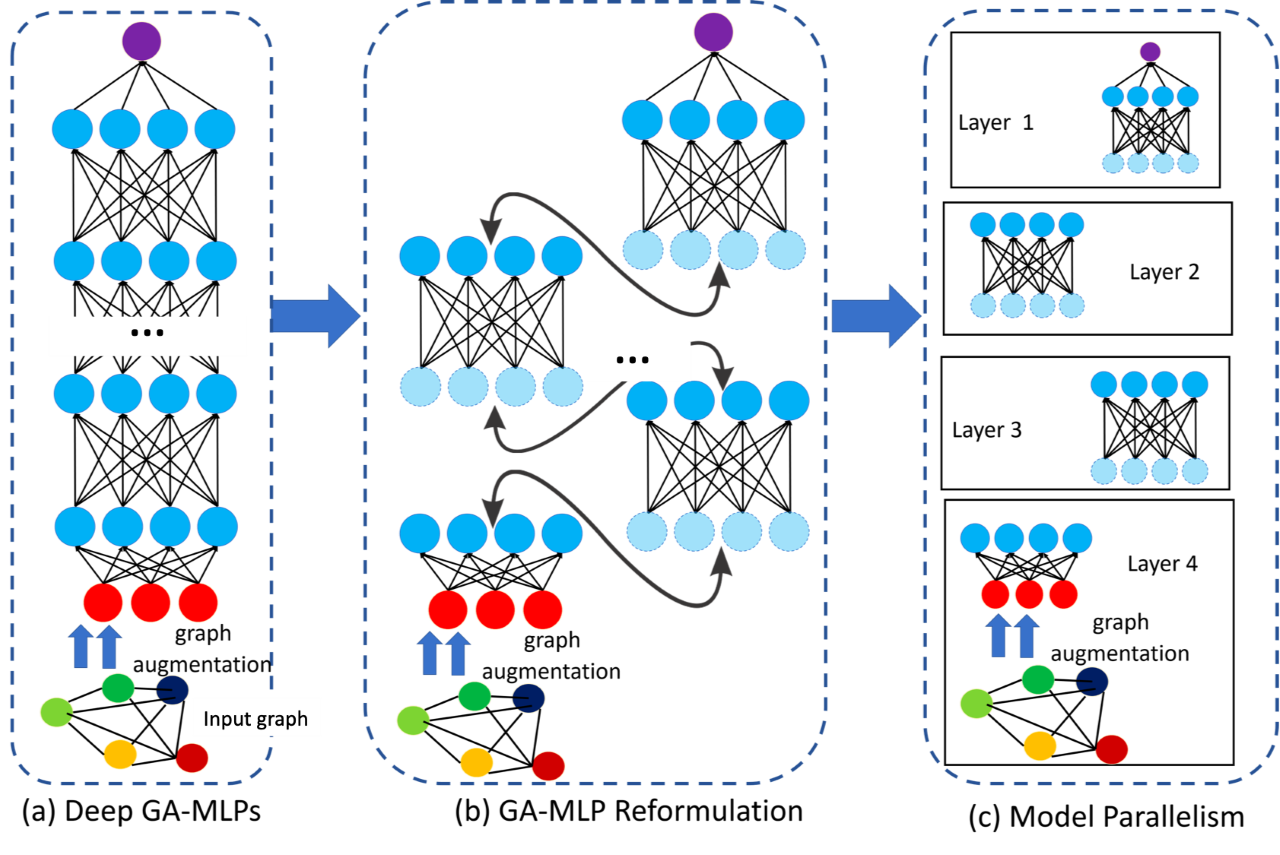
Figure 1: The overall pdADMM-G optimization algorithm: it splits GA-MLP models into layerwise components.

Algorithm 1 The pdADMM-G Algorithm to Solve Problem 2

0:  $y$, $p_{1}=X$, $\rho$, $\nu$.

0:  $\textbf{p},\textbf{W},\textbf{b},\textbf{z},\textbf{q}$.

  Initialize $k=0$.

  while $\textbf{p}^{k},\textbf{W}^{k},\textbf{b}^{k},\textbf{z}^{k},\textbf{q}^{k}$ not converged do

     $p^{k+1}_{l}\leftarrow\arg\min\nolimits_{p_{l}}L_{\rho}(\textbf{p},\textbf{W}^{k},\textbf{b}^{k},\textbf{z}^{k},\textbf{q}^{k},\textbf{u}^{k})$ for different $l$ in parallel.

     $W^{k+1}_{l}\leftarrow\arg\min\nolimits_{W_{l}}L_{\rho}(\textbf{p}^{k+1},\textbf{W},\textbf{b}^{k},\textbf{z}^{k},\textbf{q}^{k},\textbf{u}^{k})$ for different $l$ in parallel.

     $b^{k+1}_{l}\leftarrow\arg\min\nolimits_{b_{l}}L_{\rho}(\textbf{p}^{k+1},\textbf{W}^{k+1},\textbf{b},\textbf{z}^{k},\textbf{q}^{k},\textbf{u}^{k})$ for different $l$ in parallel.

     $z^{k+1}_{l}\leftarrow\arg\min\nolimits_{z_{l}}L_{\rho}(\textbf{p}^{k+1},\textbf{W}^{k+1},\textbf{b}^{k+1},\textbf{z},\textbf{q}^{k},\textbf{u}^{k})$ for different $l$ in parallel.

     $q^{k+1}_{l}\leftarrow\arg\min\nolimits_{q_{l}}L_{\rho}(\textbf{p}^{k+1},\textbf{W}^{k+1},\textbf{b}^{k+1},\textbf{z}^{k+1},\textbf{q},\textbf{u}^{k})$ for different $l$ in parallel.

     $r^{k}_{l}\leftarrow p^{k+1}_{l+1}-q^{k+1}_{l}(l=1,\cdots,L)$ in parallel # Compute residuals.

     $u^{k+1}_{l}\leftarrow u^{k}_{l}+\rho(p^{k+1}_{l+1}-q^{k+1}_{l})$ for different $l$ in parallel.

     $k\leftarrow k+1$.

  end while

  Output $\textbf{p},\textbf{W},\textbf{b},\textbf{z},\textbf{q}$.

Due to space limit, the details of all subproblems are shown in Section -A in the Appendix.
Our proposed pdADMM-G algorithm can be efficient for training deep GA-MLP models via the greedy layerwise training strategy [31]. Specifically, we begin by training a shallow GA-MLP model. Next, more layers are increased to the GA-MLP model and their parameters are trained, then we introduce even more layers and iterate this process until the whole deep GA-MLP model is included. The pdADMM-G algorithm can achieve excellent performance as well as reduce training costs by this strategy.
Last but not least, we compare the computational costs of the proposed pdADMM-G algorithm with the state-of-the-art backpropagation algorithm, on which the gradient descent is based. We show that they share the same level of computational costs. For the backpropagation algorithm, the most costly operation is the matrix multiplication $z_{l}=W_{l}p_{l}+b_{l}$ in the forward pass, where $W_{l}\in\mathbb{R}^{n_{l}\times n_{l-1}}$ and $p_{l}\in\mathbb{R}^{n_{l-1}\times|V|}$, which requires a time complexity of $O(n_{l}n_{l-1}|V|)$ [32]; for the proposed pdADMM-G algorithm, the most costly operation is to compute the derivative $\nabla_{W_{l}}\phi$, and it also involves the matrix multiplication, and hence its time complexity is again $O(n_{l}n_{l-1}|V|)$. However, the proposed pdADMM-G algorithm trains the whole GA-MLP model in a model parallelism fashion [33], and therefore all computational costs can be split into different independent clients for parallel training; whereas the backpropagation algorithm is implemented sequentially, and thus it is less efficient than the proposed pdADMM-G algorithm.

III-C Quantization Extension of pdADMM-G (pdADMM-G-Q)

In the proposed pdADMM-G algorithm, $p_{l}$ and $q_{l}$ are transmitted back and forth among layers (i.e. clients). However, the communication overheads of $p_{l}$ and $q_{l}$ surge for a large-scale graph $G$ with millions of nodes. To alleviate this challenge, the quantization technique is commonly utilized to reduce communication costs by mapping continuous values into a discrete set [34]. In other words, $p_{l}$ is required to fit into a countable set $\Delta$, which is shown as follows:

Problem 3.

$$\min\nolimits_{\textbf{p},\textbf{W},\textbf{b},\textbf{z},\textbf{q}}F(\textbf{p},\textbf{W},\textbf{b},\textbf{z},\textbf{q})=R(z_{L};y)$$

$$+(\nu/2)(\sum\nolimits_{l=1}^{L}\|z_{l}-W_{l}p_{l}-b_{l}\|^{2}_{2}+\sum\nolimits_{l=1}^{L-1}\|q_{l}-f_{l}(z_{l})\|^{2}_{2}),$$

$$s.t.\ p_{l+1}=q_{l},\ p_{l}\in\Delta=\{\delta_{1},\cdots,\delta_{m}\},$$

where $\delta_{i}(i=1,\cdots,m)\in\Delta$ are quantized values, which can be integers or low-precision values. $m=|\Delta|$ is the cardinality of $\Delta$. To address Problem 3, we rewrite it into the following form:

$$\min\nolimits_{\textbf{p},\textbf{W},\textbf{b},\textbf{z},\textbf{q}}R(z_{L};y)+\sum\nolimits_{l=2}^{L}\mathbb{I}(p_{l})$$

$$+(\nu/2)(\sum\nolimits_{l=1}^{L}\|z_{l}-W_{l}p_{l}-b_{l}\|^{2}_{2}+\sum\nolimits_{l=1}^{L-1}\|q_{l}-f_{l}(z_{l})\|^{2}_{2}),$$

$$s.t.\ p_{l+1}=q_{l},$$

where the indicator function $\mathbb{I}(p_{l})$ is defined as follows: $\mathbb{I}(p_{l})=0$ if $p_{l}\in\Delta$, and $\mathbb{I}(p_{l})=+\infty$ if $p_{l}\not\in\Delta$. The augmented Lagrangian of Problem 3 is shown as follows:

$$\beta_{\rho}(\textbf{p},\textbf{W},\textbf{b},\textbf{z},\textbf{q},\textbf{u})=L_{\rho}(\textbf{p},\textbf{W},\textbf{b},\textbf{z},\textbf{q},\textbf{u})+\sum\nolimits_{l=2}^{L}\mathbb{I}(p_{l}),$$

where $L_{\rho}$ is the augmented Lagrangian of Problem 2. The extended pdADMM-G-Q algorithm follows the same routine as the pdADMM-G algorithm, where $L_{\rho}$ is replaced with $\beta_{\rho}$. Due to space limit, the solutions to all subproblems generated by two proposed algorithms are shown in Section -B in the Appendix.

IV Convergence Analysis

In this section, the theoretical convergence of the proposed pdADMM-G algorithm and the pdADMM-G-Q algorithm is provided. Due to space limit, we only provide sketches of proofs in this section, and their details are available in Section -C in the Appendix. Our problem formulations are more difficult than existing ADMM literature: the term $\|q_{l}-f_{l}(z_{l})\|^{2}_{2}$ is coupled in the objective, while it is separable in the existing ADMM formulations. To address this, we impose a mild condition that $\partial f_{l}(z_{l})$ is bounded in Assumption 1, and prove that $u_{l}$ is controlled via $q_{l}$ and $z_{l}$ in Lemma 5 in Section -C in the Appendix.
Firstly, the proper function, Lipschitz continuity, and coercivity are defined as follows:

Definition 1 (Proper Functions).

[35]. For a convex function $g(x):\mathbb{R}\rightarrow\mathbb{R}\bigcup\{\pm\infty\}$, $g$ is called proper if $\forall x\in\mathbb{R}$, $g(x)>-\infty$, and $\exists x_{0}\in\mathbb{R}$ such that $g(x_{0})<+\infty$.

Definition 2.

(Lipschitz Continuity) A function $g(x)$ is Lipschitz continuous if there exists a constant $D>0$ such that $\forall x_{1},x_{2}$, the following holds

$$\|g(x_{1})-g(x_{2})\|\leq D\|x_{1}-x_{2}\|.$$

Definition 3.

(Coercivity) A function $h(x)$ is coerce over the feasible set $\mathscr{F}$ means that $h(x)\rightarrow\infty$ if $x\in\mathscr{F}$ and $\|x\|\rightarrow\infty$.

Next, the definition of a quantized stationary point [34] is shown as follows:

Definition 4.

(Quantized Stationary Point) The $p_{l}$ is a quantized stationary point of of Problem 3 if there exists $\tau>0$ such that

$$p_{l}\in\arg\min\nolimits_{\delta\in\Delta}\|\delta-(p_{l}-\nabla_{p_{l}}F(\textbf{p},\textbf{W},\textbf{b},\textbf{z},\textbf{q})/\tau)\|.$$

The quantized stationary point is an extension of the stationary point in the discrete setting, and any global solution $p_{l}$ to Problem 3 is a quantized stationary point to Problem 3 (Lemma 3.7 in [34]). Then the following assumption is required for convergence analysis.

Assumption 1.

$f_{l}(z_{l})$ is Lipschitz continuous with coefficient $S>0$, $R(Z_{L};y)$ is proper, and $F(\textbf{p},\textbf{W},\textbf{b},\textbf{z},\textbf{q})$ is coercive. Moreover, $\partial f_{l}(z_{l})$ is bounded, i.e. there exists $M>0$ such that $\|\partial f_{l}(z_{l})\|\leq M$.

Assumption 1 is mild to satisfy: most common activation functions such as Rectified Linear Unit (ReLU) [33] and leaky ReLU[36] satisfy Assumption 1. The risk function $R(z_{l};y)$ is only required to be proper, which shows that the convergence condition of our proposed pdADMM-G is milder than that of the dlADMM, which requires $R(z_{l};y)$ to be Lipschitz differentiable [7]. Due to the space limit, detailed proofs are provided in Section -C in the Appendix. The technical proofs follow a similar routine as dlADMM [7]. The difference consists in the fact that the dual variable $u_{l}$ is controlled by $q_{l}$ and $z_{l}$ (Lemma 6 in Section -C in the Appendix), which holds under Assumption 1, while $u_{l}$ can be controlled only by $z_{l}$ in the convergence proof of dlADMM. The first lemma shows that the objective keeps decreasing when $\rho$ is sufficiently large.

Lemma 1 (Objective Decrease).

For both the pdADMM-G algorithm and the pdADMM-G-Q algorithm, if $\rho>\max(4\nu S^{2},(\sqrt{17}+1)\nu/2)$, there exist $C_{1}=\nu/2-2\nu^{2}S^{2}/\rho>0$ and $C_{2}=\rho/2-2\nu^{2}/\rho-\nu/2>0$ such that it holds for any $k\in\mathbb{N}$ that

$$L_{\rho}(\textbf{p}^{k},\!\textbf{W}^{k},\!\textbf{b}^{k},\!\textbf{z}^{k},\!\textbf{q}^{k},\!\textbf{u}^{k})\!-\!L_{\rho}(\textbf{p}^{k\!+\!1},\textbf{W}^{k\!+\!1},\textbf{b}^{k\!+\!1},\textbf{z}^{k\!+\!1},\textbf{q}^{k\!+\!1},\textbf{u}^{k\!+\!1})$$

$$\geq\sum\nolimits_{l\!=\!2}^{L}(\tau^{k\!+\!1}_{l}/2)\|p^{k+1}_{l}\!-\!p^{k}_{l}\|^{2}_{2}\!+\!\sum\nolimits_{l\!=\!1}^{L}(\theta^{k\!+\!1}_{l}/2)\|W^{k\!+\!1}_{l}\!-\!W^{k}_{l}\|^{2}_{2}\!$$

$$\!+\!\sum\nolimits_{l\!=\!1}^{L}(\nu/2)\|b^{k\!+\!1}_{l}\!-\!b^{k}_{l}\|^{2}_{2}\!+\!\sum\nolimits_{l\!=\!1}^{L\!-\!1}C_{1}\|z^{k+1}_{l}\!-\!z^{k}_{l}\|^{2}_{2}$$

$$\!+\!(\nu/2)\|z^{k+1}_{L}-z^{k}_{L}\|^{2}_{2}+\sum\nolimits_{l=1}^{L-1}C_{2}\|q^{k+1}_{l}-q^{k}_{l}\|^{2}_{2},$$ (1)

$$\beta_{\rho}(\textbf{p}^{k},\!\textbf{W}^{k},\!\textbf{b}^{k},\!\textbf{z}^{k},\!\textbf{q}^{k},\!\textbf{u}^{k})\!-\!\beta_{\rho}(\textbf{p}^{k\!+\!1},\textbf{W}^{k\!+\!1},\textbf{b}^{k\!+\!1},\textbf{z}^{k\!+\!1},\textbf{q}^{k\!+\!1},\textbf{u}^{k\!+\!1})$$

$$\geq\!\sum\nolimits_{l\!=\!1}^{L}(\theta^{k\!+\!1}_{l}/2)\|W^{k\!+\!1}_{l}\!-\!W^{k}_{l}\|^{2}_{2}\!+\!\sum\nolimits_{l\!=\!1}^{L}(\nu/2)\|b^{k\!+\!1}_{l}\!-\!b^{k}_{l}\|^{2}_{2}\!$$

$$+\!\sum\nolimits_{l\!=\!1}^{L\!-\!1}C_{1}\|z^{k+1}_{l}\!-\!z^{k}_{l}\|^{2}_{2}+\!(\nu/2)\|z^{k+1}_{L}-z^{k}_{L}\|^{2}_{2}$$

$$+\sum\nolimits_{l=1}^{L-1}C_{2}\|q^{k+1}_{l}-q^{k}_{l}\|^{2}_{2}.$$ (2)

Sketch of Proof.

They can be proven via the optimality conditions of all subproblems, and Assumption 1. ∎

Lemma 2 shows that the objective is bounded from below when $\rho$ is large enough, and all variables are bounded.

Lemma 2 (Bounded Objective).

(1). For the pdADMM-G algorithm, if $\rho>\nu$, then $L_{\rho}(\textbf{p}^{k},\textbf{W}^{k},\textbf{b}^{k},\textbf{z}^{k},\textbf{q}^{k},\textbf{u}^{k})$ is lower bounded. Moreover, $\textbf{p}^{k},\textbf{W}^{k},\textbf{b}^{k},\textbf{z}^{k},\textbf{q}^{k}$,and $\textbf{u}^{k}$ are bounded, i.e. there exist $\mathbb{N}_{\textbf{p}}$, $\mathbb{N}_{\textbf{W}}$, $\mathbb{N}_{\textbf{b}}$, $\mathbb{N}_{\textbf{z}}$, $\mathbb{N}_{\textbf{q}}$, and $\mathbb{N}_{\textbf{u}}>0$, such that $\|\textbf{p}^{k}\|\leq\mathbb{N}_{\textbf{p}}$, $\|\textbf{W}^{k}\|\leq\mathbb{N}_{\textbf{W}}$, $\|\textbf{b}^{k}\|\leq\mathbb{N}_{\textbf{b}}$, $\|\textbf{z}^{k}\|\leq\mathbb{N}_{\textbf{z}}$, $\|\textbf{q}^{k}\|\leq\mathbb{N}_{\textbf{q}}$, and $\|\textbf{u}^{k}\|\leq\mathbb{N}_{\textbf{u}}$.
(2). For the pdADMM-G-Q algorithm, if $\rho>\nu$, then $\beta_{\rho}(\textbf{p}^{k},\textbf{W}^{k},\textbf{b}^{k},\textbf{z}^{k},\textbf{q}^{k},\textbf{u}^{k})$ is lower bounded. Moreover, $\textbf{W}^{k},\textbf{b}^{k},\textbf{z}^{k},\textbf{q}^{k}$,and $\textbf{u}^{k}$ are bounded, i.e. there exist $\overline{\mathbb{N}}_{\textbf{W}}$, $\overline{\mathbb{N}}_{\textbf{b}}$, $\overline{\mathbb{N}}_{\textbf{z}}$, $\overline{\mathbb{N}}_{\textbf{q}}$, and $\overline{\mathbb{N}}_{\textbf{u}}>0$, such that $\|\textbf{W}^{k}\|\leq\overline{\mathbb{N}}_{\textbf{W}}$, $\|\textbf{b}^{k}\|\leq\overline{\mathbb{N}}_{\textbf{b}}$, $\|\textbf{z}^{k}\|\leq\overline{\mathbb{N}}_{\textbf{z}}$, $\|\textbf{q}^{k}\|\leq\overline{\mathbb{N}}_{\textbf{q}}$, and $\|\textbf{u}^{k}\|\leq\overline{\mathbb{N}}_{\textbf{u}}$.

Sketch of Proof.

We only show the sketch proof of (1) because (2) follows the same routine as (1). In order to prove the boundness of $L_{\rho}$, we should prove the following:

$$L_{\rho}(\textbf{p}^{k},\textbf{W}^{k},\textbf{b}^{k},\textbf{z}^{k},\textbf{q}^{k},\textbf{u}^{k})$$

$$\geq F(\textbf{p}^{k},\textbf{W}^{k},\textbf{b}^{k},\textbf{z}^{k},\textbf{q}^{{}^{\prime}})+((\rho-\nu)/2)\|p^{k}_{l+1}-q^{k}_{l}\|^{2}_{2}$$

$$>-\infty,$$

where $p^{k}_{l+1}=q^{{}^{\prime}}_{l}$. Therefore, $F(\textbf{p}^{k},\textbf{W}^{k},\textbf{b}^{k},\textbf{z}^{k},\textbf{q}^{{}^{\prime}})$ and $((\rho-\nu)/2)\|p^{k}_{l+1}-q^{k}_{l}\|^{2}_{2}$ are upper bounded by $L_{\rho}(\textbf{p}^{k},\textbf{W}^{k},\textbf{b}^{k},\textbf{z}^{k},\textbf{q}^{k},\textbf{u}^{k})$ and hence $L_{\rho}(\textbf{p}^{0},\textbf{W}^{0},\textbf{b}^{0},\textbf{z}^{0},\textbf{q}^{0},\textbf{u}^{0})$ (Lemma 1). The boundness of variables can be obtained via Assumption 1. ∎

Based on Lemmas 1 and 2, the following theorem ensures that the objective is convergent.

Theorem 1 (Convergent Objective).

(1). For the pdADMM-G algorithm, if $\rho>\max(4\nu S^{2},(\sqrt{17}+1)\nu/2)$, then $L_{\rho}(\textbf{p}^{k},\textbf{W}^{k},\textbf{b}^{k},\textbf{z}^{k},\textbf{q}^{k},\textbf{u}^{k})$ is convergent. Moreover, $\lim_{k\rightarrow\infty}\|\textbf{p}^{k+1}-\textbf{p}^{k}\|^{2}_{2}=0$, $\lim_{k\rightarrow\infty}\|\textbf{W}^{k+1}-\textbf{W}^{k}\|^{2}_{2}=0$, $\lim_{k\rightarrow\infty}\|\textbf{b}^{k+1}-\textbf{b}^{k}\|^{2}_{2}=0$, $\lim_{k\rightarrow\infty}\|\textbf{z}^{k+1}-\textbf{z}^{k}\|^{2}_{2}=0$, $\lim_{k\rightarrow\infty}\|\textbf{q}^{k+1}-\textbf{q}^{k}\|^{2}_{2}=0$, $\lim_{k\rightarrow\infty}\|\textbf{u}^{k+1}-\textbf{u}^{k}\|^{2}_{2}=0$.
(2). For the pdADMM-G-Q algorithm, if $\rho>\max(4\nu S^{2},(\sqrt{17}+1)\nu/2)$, then $\beta_{\rho}(\textbf{p}^{k},\textbf{W}^{k},\textbf{b}^{k},\textbf{z}^{k},\textbf{q}^{k},\textbf{u}^{k})$ is convergent. Moreover, $\lim_{k\rightarrow\infty}\|\textbf{W}^{k+1}-\textbf{W}^{k}\|^{2}_{2}=0$, $\lim_{k\rightarrow\infty}\|\textbf{b}^{k+1}-\textbf{b}^{k}\|^{2}_{2}=0$, $\lim_{k\rightarrow\infty}\|\textbf{z}^{k+1}-\textbf{z}^{k}\|^{2}_{2}=0$, $\lim_{k\rightarrow\infty}\|\textbf{q}^{k+1}-\textbf{q}^{k}\|^{2}_{2}=0$, $\lim_{k\rightarrow\infty}\|\textbf{u}^{k+1}-\textbf{u}^{k}\|^{2}_{2}=0$.

Sketch of Proof.

This theorem can be derived by taking the limit on both sides of Inequality (1). ∎

The third lemma guarantees that the subgradient of the objective is upper bounded, which is stated as follows:

Lemma 3 (Bounded Subgradient).

(1). For the pdADMM-G algorithm, there exists a constant $C>0$ and $g^{k+1}\in\partial L_{\rho}(\textbf{p}^{k+1},\textbf{W}^{k+1},\textbf{b}^{k+1},\textbf{z}^{k+1},\textbf{q}^{k+1},\textbf{u}^{k+1})$ such that

$$\|g^{k+1}\|\leq C(\|\textbf{p}^{k+1}-\textbf{p}^{k}\|+\|\textbf{W}^{k+1}-\textbf{W}^{k}\|+\|\textbf{b}^{k+1}-\textbf{b}^{k}\|$$

$$+\|\textbf{z}^{k+1}-\textbf{z}^{k}\|+\|\textbf{q}^{k+1}-\textbf{q}^{k}\|+\|\textbf{u}^{k+1}-\textbf{u}^{k}\|).$$

(2). For the pdADMM-G-Q algorithm, there exists a constant $\overline{C}>0$, $\overline{g}_{\textbf{W}}^{k+1}\in\nabla_{\textbf{W}^{k+1}}\beta_{\rho}(\textbf{p}^{k+1},\textbf{W}^{k+1},\textbf{b}^{k+1},\textbf{z}^{k+1},\textbf{q}^{k+1},\textbf{u}^{k+1})$, $\overline{g}_{\textbf{b}}^{k+1}\in\nabla_{\textbf{b}^{k+1}}\beta_{\rho}(\textbf{p}^{k+1},\textbf{W}^{k+1},\textbf{b}^{k+1},\textbf{z}^{k+1},\textbf{q}^{k+1},\textbf{u}^{k+1})$, $\overline{g}_{\textbf{z}}^{k+1}\in\partial_{\textbf{z}^{k+1}}\beta_{\rho}(\textbf{p}^{k+1},\textbf{W}^{k+1},\textbf{b}^{k+1},\textbf{z}^{k+1},\textbf{q}^{k+1},\textbf{u}^{k+1})$, $\overline{g}_{\textbf{q}}^{k+1}\in\nabla_{\textbf{q}^{k+1}}\beta_{\rho}(\textbf{p}^{k+1},\textbf{W}^{k+1},\textbf{b}^{k+1},\textbf{z}^{k+1},\textbf{q}^{k+1},\textbf{u}^{k+1})$, $\overline{g}_{\textbf{u}}^{k+1}\in\nabla_{\textbf{u}^{k+1}}\beta_{\rho}(\textbf{p}^{k+1},\textbf{W}^{k+1},\textbf{b}^{k+1},\textbf{z}^{k+1},\textbf{q}^{k+1},\textbf{u}^{k+1})$ such that

$$\|\overline{g}_{\textbf{W}}^{k+1}\|\leq\overline{C}(\|\textbf{W}^{k+1}-\textbf{W}^{k}\|+\|\textbf{b}^{k+1}-\textbf{b}^{k}\|$$

$$+\|\textbf{z}^{k+1}-\textbf{z}^{k}\|+\|\textbf{q}^{k+1}-\textbf{q}^{k}\|+\|\textbf{u}^{k+1}-\textbf{u}^{k}\|),$$

$$\|\overline{g}_{\textbf{b}}^{k+1}\|\leq\overline{C}(\|\textbf{W}^{k+1}-\textbf{W}^{k}\|+\|\textbf{b}^{k+1}-\textbf{b}^{k}\|$$

$$+\|\textbf{z}^{k+1}-\textbf{z}^{k}\|+\|\textbf{q}^{k+1}-\textbf{q}^{k}\|+\|\textbf{u}^{k+1}-\textbf{u}^{k}\|),$$

$$\|\overline{g}_{\textbf{z}}^{k+1}\|\leq\overline{C}(\|\textbf{W}^{k+1}-\textbf{W}^{k}\|+\|\textbf{b}^{k+1}-\textbf{b}^{k}\|$$

$$+\|\textbf{z}^{k+1}-\textbf{z}^{k}\|+\|\textbf{q}^{k+1}-\textbf{q}^{k}\|+\|\textbf{u}^{k+1}-\textbf{u}^{k}\|),$$

$$\|\overline{g}_{\textbf{q}}^{k+1}\|\leq\overline{C}(\|\textbf{W}^{k+1}-\textbf{W}^{k}\|+\|\textbf{b}^{k+1}-\textbf{b}^{k}\|$$

$$+\|\textbf{z}^{k+1}-\textbf{z}^{k}\|+\|\textbf{q}^{k+1}-\textbf{q}^{k}\|+\|\textbf{u}^{k+1}-\textbf{u}^{k}\|),$$

$$\|\overline{g}_{\textbf{u}}^{k+1}\|\leq\overline{C}(\|\textbf{W}^{k+1}-\textbf{W}^{k}\|+\|\textbf{b}^{k+1}-\textbf{b}^{k}\|$$

$$+\|\textbf{z}^{k+1}-\textbf{z}^{k}\|+\|\textbf{q}^{k+1}-\textbf{q}^{k}\|+\|\textbf{u}^{k+1}-\textbf{u}^{k}\|).$$

Sketch of Proof.

To prove this lemma, the subgradient is proven to be upper bounded by the linear combination of $\|\textbf{p}^{k+1}-\textbf{p}^{k}\|$, $\|\textbf{W}^{k+1}-\textbf{W}^{k}\|$, $\|\textbf{b}^{k+1}-\textbf{b}^{k}\|$, $\|\textbf{z}^{k+1}-\textbf{z}^{k}\|$, $\|\textbf{q}^{k+1}-\textbf{q}^{k}\|$, and $\|\textbf{u}^{k+1}-\textbf{u}^{k}\|$. ∎

Now based on Theorem 1, and Lemma 3, the convergence of the pdADMM-G algorithm to a stationary point is presented in the following theorem.

Theorem 2 (Convergence of the pdADMM-G algorithm).

If $\rho>\max(4\nu S^{2},(\sqrt{17}+1)\nu/2)$, then for the variables $(\textbf{p},\textbf{W},\textbf{b},\textbf{z},\textbf{q},\textbf{u})$ in Problem 2, starting from any $(\textbf{p}^{0},\textbf{W}^{0},\textbf{b}^{0},\textbf{z}^{0},\textbf{q}^{0},\textbf{u}^{0})$, $(\textbf{p}^{k},\textbf{W}^{k},\textbf{b}^{k},\textbf{z}^{k},\textbf{q}^{k},\textbf{u}^{k})$ has at least a limit point $(\textbf{p}^{*},\textbf{W}^{*},\textbf{b}^{*},\textbf{z}^{*},\textbf{q}^{*},\textbf{u}^{*})$, and any limit point is a stationary point of Problem 2. That is, $0\in\partial L_{\rho}(\textbf{p}^{*},\textbf{W}^{*},\textbf{b}^{*},\textbf{z}^{*},\textbf{q}^{*},\textbf{u}^{*})$. In other words,

$$p^{*}_{l+1}=q^{*}_{l},\ \nabla_{\textbf{p}^{*}}L_{\rho}(\textbf{p}^{*},\textbf{W}^{*},\textbf{b}^{*},\textbf{z}^{*},\textbf{q}^{*},\textbf{u}^{*})\!=\!0,$$

$$\ \nabla_{\textbf{W}^{*}}\!L_{\rho}\!(\textbf{p}^{*}\!,\!\textbf{W}^{*}\!,\!\textbf{b}^{*},\textbf{z}^{*},\textbf{q}^{*},\textbf{u}^{*})\!=\!0,\nabla_{\textbf{b}^{*}}\!L_{\rho}\!(\textbf{p}^{*}\!,\!\textbf{W}^{*}\!,\!\textbf{b}^{*},\textbf{z}^{*},\textbf{q}^{*},\textbf{u}^{*})\!=\!0,$$

$$0\!\in\!\partial_{\textbf{z}^{*}}\!L_{\rho}\!(\textbf{p}^{*},\!\textbf{W}^{*},\textbf{b}^{*},\textbf{z}^{*},\textbf{q}^{*},\textbf{u}^{*}),\!\nabla_{\textbf{q}^{*}}L_{\rho}\!(\textbf{p}^{*},\!\textbf{W}^{*},\textbf{b}^{*},\textbf{z}^{*},\textbf{q}^{*},\textbf{u}^{*})\!=\!0.$$

Sketch of Proof.

This theorem can be derived directly from Lemma 2 and Lemma 3. ∎

Theorem 2 shows that our proposed pdADMM-G algorithm converges for sufficiently large $\rho$, which is consistent with previous literature [7]. Similarly, the convergence of the proposed pdADMM-G-Q algorithm is shown as follows:

Theorem 3 (Convergence of the pdADMM-G-Q algorithm).

If $\rho>\max(4\nu S^{2},(\sqrt{17}+1)\nu/2)$, then for the variables $(\textbf{p},\textbf{W},\textbf{b},\textbf{z},\textbf{q},\textbf{u})$ in Problem 3, starting from any $(\textbf{p}^{0},\textbf{W}^{0},\textbf{b}^{0},\textbf{z}^{0},\textbf{q}^{0},\textbf{u}^{0})$, $(\textbf{p}^{k},\textbf{W}^{k},\textbf{b}^{k},\textbf{z}^{k},\textbf{q}^{k},\textbf{u}^{k})$ has at least a limit point $(\textbf{p}^{*},\textbf{W}^{*},\textbf{b}^{*},\textbf{z}^{*},\textbf{q}^{*},\textbf{u}^{*})$, and any limit point $(\textbf{W}^{*},\textbf{b}^{*},\textbf{z}^{*},\textbf{q}^{*},\textbf{u}^{*})$ is a stationary point of Problem 3. Moreover, if $\tau^{k+1}_{l}$ is bounded, then $\textbf{p}^{*}$ is a quantized stationary point of Problem 3. That is

$$p^{*}_{l+1}=q^{*}_{l},\ \nabla_{\textbf{W}^{*}}\beta_{\rho}(\textbf{p}^{*},\textbf{W}^{*},\textbf{b}^{*},\textbf{z}^{*},\textbf{q}^{*},\textbf{u}^{*})=0,$$

$$\nabla_{\textbf{b}^{*}}\beta_{\rho}(\textbf{p}^{*},\textbf{W}^{*},\textbf{b}^{*},\textbf{z}^{*},\textbf{q}^{*},\textbf{u}^{*})=0,$$

$$0\in\partial_{\textbf{z}^{*}}\beta_{\rho}(\textbf{p}^{*},\textbf{W}^{*},\textbf{b}^{*},\textbf{z}^{*},\textbf{q}^{*},\textbf{u}^{*}),$$

$$\nabla_{\textbf{q}^{*}}\beta_{\rho}(\textbf{p}^{*},\textbf{W}^{*},\textbf{b}^{*},\textbf{z}^{*},\textbf{q}^{*},\textbf{u}^{*})=0,$$

$$p^{*}_{l}\in\arg\min\nolimits_{\delta\in\Delta}\|\delta-(p^{*}_{l}-\nabla_{p^{*}_{l}}F(\textbf{p}^{*},\textbf{W}^{*},\textbf{b}^{*},\textbf{z}^{*},\textbf{q}^{*})/\tau^{*}_{l})\|.$$

where $\tau^{*}_{l}$ is a limit point of $\tau^{k}_{l}$.

Sketch of Proof.

This theorem is proven using a similar procedure as Theorem 2, and the definition of the quantized stationary point. ∎

The only difference between Theorems 2 and 3 is that $\textbf{p}^{*}$ is a stationary point in Problem 2 and a quantized stationary point in Problem 3. Next, the following theorem ensures the sublinear convergence rate $o(1/k)$ of the proposed pdADMM-G algorithm and the pdADMM-G-Q algorithm.

Theorem 4 (Convergence Rate).

(1). For the pdADMM-G algorithm and a sequence $(\textbf{p}^{k},\textbf{W}^{k},\textbf{b}^{k},\textbf{z}^{k},\textbf{q}^{k},\textbf{u}^{k})$, define $c_{k}=\min\nolimits_{0\leq i\leq k}(\sum\nolimits_{l=2}^{L}(\tau^{i+1}_{l}/2)\|p^{i+1}_{l}\!-\!p^{i}_{l}\|^{2}_{2}+\sum\nolimits_{l\!=\!1}^{L}(\theta^{i\!+\!1}_{l}/2)\|W^{i\!+\!1}_{l}\!-\!W^{i}_{l}\|^{2}_{2}+\sum\nolimits_{l\!=\!1}^{L}(\nu/2)\|b^{i\!+\!1}_{l}\!-\!b^{i}_{l}\|^{2}_{2}+\sum\nolimits_{l=1}^{L-1}C_{1}\|z^{i+1}_{l}-z^{i}_{l}\|^{2}_{2}+(\nu/2)\|z^{i+1}_{L}-z^{i}_{L}\|^{2}_{2}+\sum\nolimits_{l=1}^{L-1}C_{2}\|q^{i+1}_{l}-q^{i}_{l}\|^{2}_{2})$ where $C_{1}=\nu/2-2\nu^{2}S^{2}/\rho>0$ and $C_{2}=\rho/2-2\nu^{2}/\rho-\nu/2>0$, then the convergence rate of $c_{k}$ is $o(1/k)$.
(2). For the pdADMM-G-Q algorithm and a sequence $(\textbf{W}^{k},\textbf{b}^{k},\textbf{z}^{k},\textbf{q}^{k},\textbf{u}^{k})$, define $d_{k}=\min\nolimits_{0\leq i\leq k}(\sum\nolimits_{l\!=\!1}^{L}(\theta^{i\!+\!1}_{l}/2)\|W^{i\!+\!1}_{l}\!-\!W^{i}_{l}\|^{2}_{2}+\sum\nolimits_{l\!=\!1}^{L}(\nu/2)\|b^{i\!+\!1}_{l}\!-\!b^{i}_{l}\|^{2}_{2}+\sum\nolimits_{l=1}^{L-1}C_{1}\|z^{i+1}_{l}-z^{i}_{l}\|^{2}_{2}+(\nu/2)\|z^{i+1}_{L}-z^{i}_{L}\|^{2}_{2}+\sum\nolimits_{l=1}^{L-1}C_{2}\|q^{i+1}_{l}-q^{i}_{l}\|^{2}_{2})$ where $C_{1}=\nu/2-2\nu^{2}S^{2}/\rho>0$ and $C_{2}=\rho/2-2\nu^{2}/\rho-\nu/2>0$, then the convergence rate of $d_{k}$ is $o(1/k)$.

Sketch of Proof.

(1). In order to prove the convergence rate $o(1/k)$, $c_{k}$ satisfies three conditions: (a) $c_{k}\geq c_{k+1}$, (b) $\sum\nolimits_{k=0}^{\infty}c_{k}$ is bounded, and (c) $c_{k}\geq 0$.
(2). $d_{k}$ can be proven using a similar procedure as (1). ∎

V Experiments

In this section, we evaluate the performance of the proposed pdADMM-G algorithm and the proposed pdADMM-G-Q algorithm on GA-MLP models using nine benchmark datasets. Convergence and computational overheads are demonstrated on different datasets. Speedup and test performance are compared with several state-of-the-art optimizers. All experiments were conducted on the Amazon Web Services (AWS) p2.16xlarge instance, with 16 NVIDIA K80 GPUs, 64vCPUs, a processor Intel(R) Xeon(R) CPU E5-2686 v4 @ 2.30GHz, and 732GiB of RAM.

Dataset	Node#	Edge#	Class#	Feature#	Training Set#	Validation Set#	Test Set#
Cora	$2485$	$10556$	$7$	$1433$	$140$	$500$	$1000$
PubMed	$19717$	$88648$	$3$	$500$	$60$	$500$	$1000$
Citeseer	$2110$	$9104$	$6$	$3703$	$120$	$500$	$1000$
Amazon Computers	$13381$	$491722$	$10$	$767$	$200$	$1000$	$1000$
Amazon Photo	$7487$	$238162$	$8$	$745$	$160$	$1000$	$1000$
Coauthor CS	$18333$	$163788$	$15$	$6805$	$300$	$1000$	$1000$
Coauthor Physics	$34493$	$495924$	$5$	$8415$	$100$	$1000$	$1000$
Flickr	$89250$	$899756$	$7$	$500$	$44625$	$22312$	$22313$
Ogbn-Arxiv	$169343$	$1166243$	$40$	$128$	$90941$	$29799$	$48603$

TABLE II: Dataset statistics.

V-A Datasets and Settings

Nine benchmark datasets were used for experimental evaluation, whose statistics are shown in Table II. Each dataset is split into a training set, a validation set, and a test set. Due to space limit, their details can be found in Section -D1 in the Appendix.
When it comes to experimental settings, we set $K=4$ for the multi-hop operator $\Psi$, and defined a diagonal degree matrix $D$ where $D_{ii}=\sum\nolimits_{j=1}^{|V|}A_{ij}$, and a renormalized adjacency matrix $\tilde{A}=(D+I)^{-1/2}(A+I)(D+I)^{-1/2}\in\mathbb{R}^{|V|\times|V|}$[1]. Moreover, we set $\Psi=\{I,\tilde{A},\tilde{A}^{2},\tilde{A}^{3}\}$ [2]. For all GA-MLP models, the activation function was set to ReLU. The loss function was set to the cross-entropy loss. For the pdADMM-G-Q algorithm, $\Delta=\{-1,0,1,\cdots,20\}$ in Problem 3, and p was quantized by default.

V-B Comparison Methods

GD and its variants are state-of-the-art optimizers and hence served as comparison methods. For GD-based methods, all datasets were used for training models in a full-batch fashion. All hyperparameters were chosen by maximizing the performance of validation sets. Due to space limit, hyperparameter settings of all methods are shown in Section -D2 in the Appendix. The following are their brief introductions:
1. Gradient Descent (GD) [37]. The GD and its variants are the most popular deep learning optimizers. The GD updates parameters simply based on their gradients.
2. Adaptive learning rate method (Adadelta) [38]. The Adadelta is proposed to overcome the sensitivity to hyperparameter selection.
3. Adaptive gradient algorithm (Adagrad) [39]. Adagrad is an improved version of GD: rather than fixing the learning rate during training, it adapts the learning rate to the hyperparameter.
4. Adaptive momentum estimation (Adam) [40]. Adam is the most popular optimization method for deep learning models. It estimates the first and second momentum in order to correct the biased gradient, and thus accelerates empirical convergence.

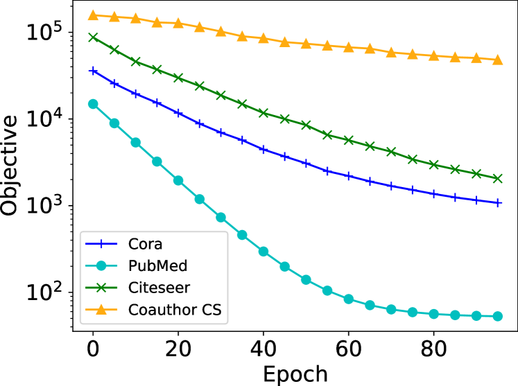
(a). pdADMM-G Objective.

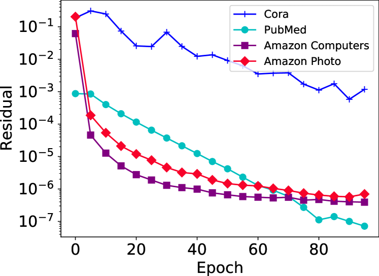
(b). pdADMM-G Residual.

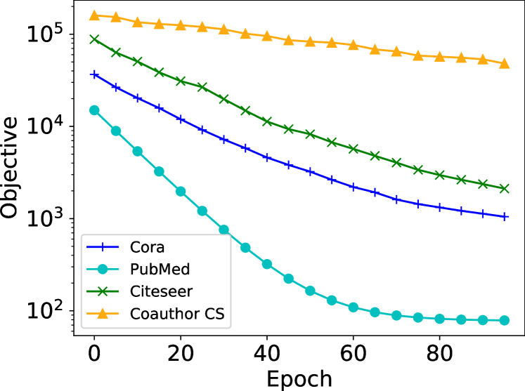
(c). pdADMM-G-Q Objective.

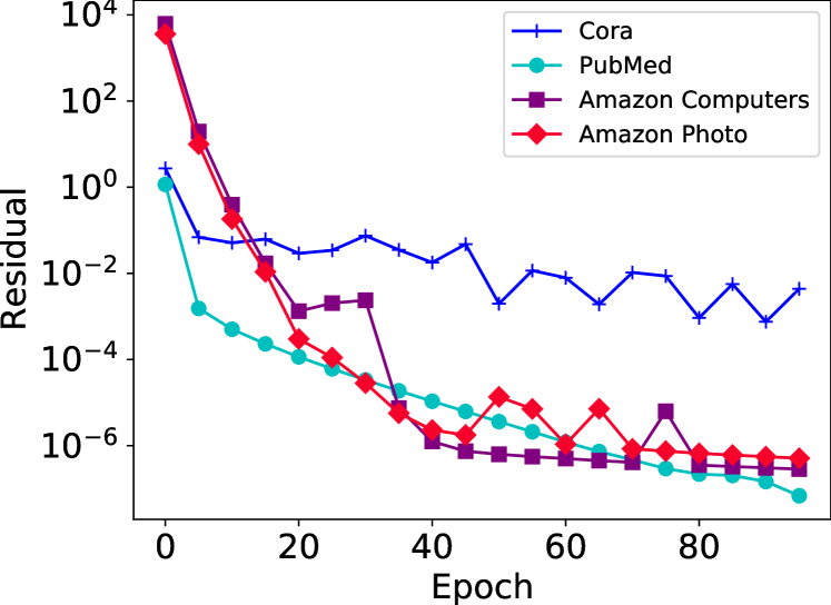
(d). pdADMM-G-Q Residual.

Figure 2: Convergence curves of the pdADMM-G algorithm and the pdADMM-G-Q algorithm in four datasets: they both converge.

V-C Convergence

Firstly, in order to validate the convergence of two proposed algorithms, we set up a GA-MLP model with $10$ layers, each of which has $1000$ neurons. The number of epochs was set to $100$. $\nu$ and $\rho$ were set to $0.01$ and $1$, respectively.
Figure 2 demonstrates objectives and residuals of two proposed algorithms on four datasets. Overall, the objectives and residuals of the two proposed algorithms are convergent. From Figure 2(a) and Figure 2(c), the objectives of the two proposed algorithms decrease drastically at the first $50$ epochs and then drop smoothly to the end. The objectives on the PubMed dataset achieve the lowest among all four datasets, whereas these on the Coauthor CS dataset are the highest, which still reach near $10^{5}$ at the $100$-th epoch. As for residuals, even though the residuals of the pdADMM-G-Q algorithm are higher than these of the pdADMM-G algorithm initially, they both converge sublinearly to 0, which is consistent with Theorem 2 and Theorem 3. Specifically, as shown in Figure 2(b) and Figure 2(d), the residuals on the Cora dataset decrease more slowly with fluctuation than these on other datasets, while residuals on the Amazon Computers and Amazon Photo datasets demonstrate the fastest decreasing speed at the first $40$ epochs before reaching a plateau less than $10^{-6}$. The residuals on the PubMed dataset accomplish the lowest values among all four datasets again with a value of less than $10^{-7}$.

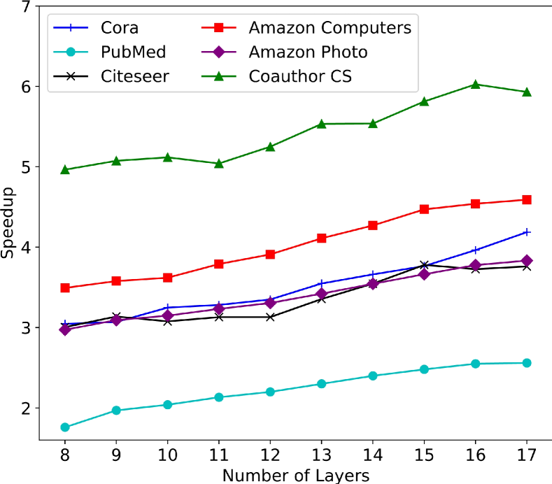
(a). The speedup

on small datasets.

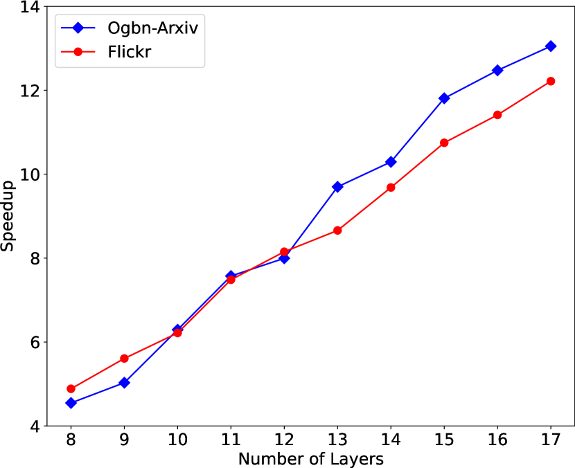
(b). The speedup

on large datasets.

Figure 3: The speedup of the proposed pdADMM-G on different datasets concerning the number of layers: the speedup increases linearly with the number of layers, and the slopes of speedups are higher on large datasets than those on small datasets.

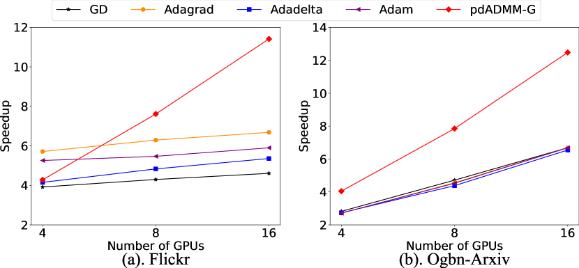
Figure 4: The speedup of all methods on two large datasets concerning the number of GPUs: speedups of the proposed pdADMM-G are higher than these of all comparison methods.

V-D Speedup

Next, we investigate the speedup of the pdADMM-G algorithm in the large deep GA-MLP models. The running time per epoch was an average of $10$ epochs. $\rho$ and $\nu$ were both set to $10^{-3}$. We investigate the speedup concerning two factors: the number of layers and the number of GPUs.
For the relationship between the speedup and the number of layers, the pdADMM-G algorithm in the GA-MLP models with $4000$ neurons was tested. The number of layers ranged from $8$ to $17$. The speedup on small datasets and large datasets are shown in Figure 3(a) and Figure 3(b), respectively. Overall, the speedup of the proposed pdADMM-G increases linearly with the number of layers. For example, the speedups on the Cora dataset and the Amazon Computers dataset rise from $3$ and $3.5$ gradually to $4$ and $4.5$, respectively. The speedup on the PubMed dataset achieves the lowest with a value of less than $3$, whereas that on the Coauthor CS dataset at least doubles that on any other small dataset, with a peak of $6$. Moreover, the speedup is more obvious on large datasets. For example, when the slopes of speedups are compared, the slope on the Flickr dataset is at least five times much steeper than that on the Coauthor CS dataset. The same trend is applied to the Ogbn-Arxiv dataset. This means that our proposed pdADMM-G algorithm is more suitable for large datasets.
For the relationship between the speedup and the number of GPUs, we set up a large GA-MLP model with $16$ layers and $4000$ neurons and kept all hyperparameters in the previous experiment. The speedup of our proposed pdADMM-G algorithm was compared with all comparison methods. Figure 4 shows all speedups on two large datasets. The proposed pdADMM-G algorithm achieves a higher speedup than any GD-based method. For example, the speedups of 8 GPUs are nearly $8$ on the Flickr dataset and the Ogbn-Arxiv dataset, while the best speedups achieved via comparison methods are in the vicinity of $6$ and $5$ on two datasets, respectively. We also observe that while speedups of all methods scale linearly with the number of GPUs, the slopes of our proposed pdADMM-G algorithm are steeper than these of any comparison method. For example, the slope of our proposed pdADMM-G algorithm on the Flickr dataset is more than 10 times steeper than that of Adam. All comparison methods show similar flat slopes, and they achieve a higher slope of the speedup on the Ogbn-Arxiv dataset than that on the Flickr dataset.
In summary, the speedup of our proposed pdADMM-G algorithm scales linearly with the number of layers and the number of GPUs. Moreover, its speedup is superior to any other comparison method significantly by more than $10$ times.

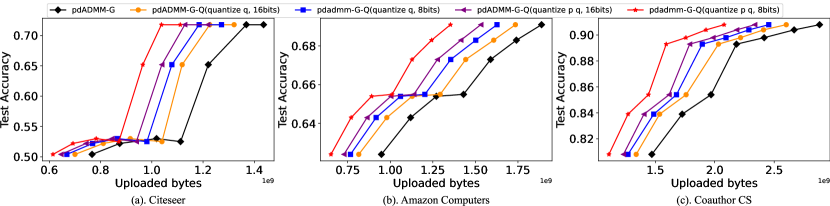
Figure 5: Communication overheads of two proposed algorithms on three datasets: the quantization concerning both p and q using $8$ bits reduces the communication overheads by up to $45\%$ without loss of performance.

V-E Communication Overheads

Then, it is necessary to explore how many communication overheads can be reduced using the proposed quantization technique on different quantization levels. To achieve this, we established a large GA-MLP model with $10$ layers, each of which consists of $1000$ neurons. We set up three quantization cases: no quantization, the quantization concerning p only, and the quantization concerning both p and q. For every quantization case, we also set up two different quantization sizes: $8$ bits and $16$ bits. Figure 5 demonstrates the relationship between the test accuracy and communication overheads for different quantization cases and sizes on three datasets. Overall, communication overheads can be reduced significantly by the proposed quantization technique. The amount of reduction depends on different quantization cases and sizes. Generally speaking, the more variables are quantized and the fewer bits are compressed, then the more savings in communications can be achieved. Take the Citeseer dataset as an example, while all algorithms reach the same test accuracy above $70\%$, the proposed pdADMM-G (i.e. no quantization) consumes the most communication costs with the value of around $1.4\times 10^{9}$ bytes. If the variable p is quantized using $16$ bits, the communication overhead drops by $10\%$, and then using $8$ bits saves another $5\%$. When variables p and q are both quantized, the communication overhead tumbles down to $1.2\times 10^{9}$ bytes, which means decreases by $16.7\%$ when it is compared with the case where only p is quantized. When variables are compressed to $8$ bits instead of $16$ bits, the communication overhead slips further to $1.1\times 10^{9}$, a nearly $30\%$ decline. The same trend is applied to the other two datasets, and they accomplish a shrink of communication overheads by $33\%$ and $45\%$, respectively. This demonstrates that our proposed quantization technique is effective for reducing unnecessary communication costs without loss of performance. We also observe that the Coauthor CS dataset is the largest dataset among the three, and it accomplishes the greatest communication reduction.

Dataset	Cora	PubMed	Citeseer
GD	0.730$\pm$0.022	0.638$\pm$ 0.080	0.637$\pm$0.040
Adadelta	0.671$\pm$0.064	0.705$\pm$0.038	0.620$\pm$0.016
Adagrad	0.726$\pm$0.025	0.753$\pm$ 0.015	0.601$\pm$0.037
Adam	0.725$\pm$0.036	0.742$\pm$0.007	0.631$\pm$0.018
pdADMM-G	0.784$\pm$0.003	0.784$\pm$0.004	0.709$\pm$0.003
pdADMM-G-Q	0.788$\pm$0.003	0.782$\pm$0.003	0.712$\pm$ 0.001
Dataset	Amazon Computers	Amazon Photo	Coauthor CS
GD	0.646$\pm$0.032	0.735$\pm$ 0.169	0.884$\pm$0.010
Adadelta	0.136$\pm$0.060	0.369$\pm$ 0.045	0.787$\pm$0.086
Adagrad	0.688$\pm$0.023	0.813$\pm$ 0.018	0.887$\pm$0.007
Adam	0.724$\pm$0.010	0.855$\pm$0.009	0.883$\pm$0.009
pdADMM-G	0.735$\pm$0.006	0.856$\pm$0.011	0.915$\pm$0.004
pdADMM-G-Q	0.687$\pm$ 0.054	0.832$\pm$0.010	0.914$\pm$0.003
Dataset	Coauthor Physics	Flickr	Ogbn-Arxiv
GD	0.909$\pm$0.007	0.466$\pm$0.007	0.361$\pm$0.063
Adadelta	0.915$\pm$0.014	0.461$\pm$0.008	0.523$\pm$ 0.030
Adagrad	0.916$\pm$0.012	0.481$\pm$0.003	0.567$\pm$0.016
Adam	0.912$\pm$0.016	0.512 $\pm$0.004	0.674$\pm$ 0.006
pdADMM-G	0.921$\pm$0.003	0.513$\pm$0.002	0.647$\pm$0.002
pdADMM-G-Q	0.919$\pm$0.002	0.507$\pm$0.003	0.655$\pm$0.002

TABLE III: The test performance of all methods when the number of neurons is 100: two proposed algorithms outperform all comparison methods.

Dataset	Cora	PubMed	Citeseer
GD	0.757$\pm$0.024	0.699$\pm$0.655	0.680$\pm$0.014
Adadelta	0.717$\pm$0.063	0.722$\pm$0.696	0.564$\pm$0.028
Adagrad	0.776$\pm$0.013	0.759$\pm$0.761	0.650 $\pm$0.038
Adam	0.771$\pm$0.020	0.778$\pm$0.767	0.662 $\pm$0.021
pdADMM-G	0.786$\pm$0.005	0.786$\pm$0.786	0.713$\pm$0.007
pdADMM-G-Q	0.786$\pm$0.005	0.788$\pm$0.787	0.712$\pm$0.005
Dataset	Amazon Computers	Amazon Photo	Coauthor CS
GD	0.707$\pm$0.012	0.817$\pm$0.005	0.906$\pm$0.005
Adadelta	0.243$\pm$0.063	0.380$\pm$0.069	0.880$\pm$0.011
Adagrad	0.753$\pm$0.009	0.866$\pm$0.007	0.911$\pm$0.003
Adam	0.739$\pm$0.022	0.880$\pm$ 0.016	0.898$\pm$0.013
pdADMM-G	0.751$\pm$0.008	0.873$\pm$0.004	0.920$\pm$0.002
pdADMM-G-Q	0.748$\pm$0.004	0.865$\pm$0.007	0.919$\pm$0.003
Dataset	Coauthor Physics	Flickr	Ogbn-Arxiv
GD	0.917$\pm$0.004	0.466$\pm$0.001	0.436$\pm$0.042
Adadelta	0.917$\pm$0.004	0.462$\pm$0.001	0.584$\pm$0.031
Adagrad	0.914$\pm$0.004	0.487$\pm$0.005	0.630$\pm$0.016
Adam	0.914$\pm$0.002	0.517$\pm$0.002	0.682$\pm$0.010
pdADMM-G	0.918$\pm$0.003	0.515$\pm$0.002	0.655$\pm$0.001
pdADMM-G-Q	0.918$\pm$0.002	0.512$\pm$0.003	0.657$\pm$0.002

TABLE IV: The test performance of all methods when the number of neurons is 500: two proposed algorithms outperform all comparison methods.

V-F Performance

Finally, we evaluate the performance of two proposed algorithms against all comparison methods on nine benchmark datasets. We set up two standard GA-MLP models with $10$ layers but different neurons: the first model has $100$ neurons, while the second model has $500$ neurons. Following the greedy layerwise training strategy [31], we firstly trained a two-layer GA-MLP model, and then three more layers were added to training, and finally, all $10$ layers were involved. The number of epochs was set to $200$. We repeated all experiments five times and reported their means and the standard deviations. Due to space limit, hyperparameter settings and the performance of validation sets are shown in Section -D2 and -D3 in the Appendix, respectively.
Table III demonstrates the performance of all methods when the number of neurons is $100$. In summary, the two proposed algorithms outperform all comparison methods slightly: they occupy the best algorithms on eight datasets out of the total nine datasets. For example, they both achieve $78\%$ test accuracy on the Cora dataset, whereas the best comparison method is GD, which only reaches $73\%$ test accuracy, and is at least $6\%$ lower than the two proposed algorithms. As another example, two proposed algorithms accomplish $78\%$ test accuracy on the PubMed dataset, $4\%$ better than that achieved by Adagrad, whose performance is the best aside from the two proposed algorithms. The Citeseer dataset shows the largest performance gap between the two proposed algorithms and all comparison methods. Two proposed algorithms reach the level of $70\%$ test accuracy, whereas all comparison methods fall in the vicinity of $60\%$ test accuracy. In other words, the two proposed algorithms outperform all comparison methods by more than $10\%$. For two proposed algorithms, the proposed pdADMM-G algorithm outperforms marginally the proposed pdADMM-G-Q algorithm due to the quantization technique. Their largest performance gap is $5\%$, which is achieved on the Amazon Computers dataset. The Adam is the best comparison method overall, and it serves as the best algorithm on the Ogbn-Arxiv dataset. The Adadelta performs the worst among all comparison methods, whose performance is significantly lower than any other method on several datasets such as the Amazon Computers dataset, the Amazon Photo dataset, and the Coauthor CS dataset. Last but not least, the standard deviations of all methods remain low, and this shows that they are robust to different initializations.
Table IV shows the performance of all methods when the number of neurons is $500$. In general, two proposed algorithms still reach a better performance than all comparison methods, but the gap is more narrow. For example, in Table III, the proposed pdADMM-G algorithm achieves the best on the Amazon Computers dataset. However, it is surpassed by Adagrad slightly in Table IV. We also observe that a GA-MLP model with $500$ neurons performs better than that with $100$ neurons, which are trained by the same algorithm. This makes sense since the wider a model is, the more expressiveness it is equipped with.

VI Conclusion

The GA-MLP models are attractive to the deep learning community due to potential resistance to some problems of GNNs such as over-smoothing and over-squashing. In this paper, we propose a novel pdADMM-G algorithm to achieve parallel training of GA-MLP models, which is accomplished by breaking the layer dependency. The extended pdADMM-G-Q algorithm reduces communication overheads by the introduction of the quantization technique. Their theoretical convergence to a (quantized) stationary point of the problem is guaranteed with a sublinear convergence rate $o(1/k)$, where $k$ is the number of iterations. Extensive experiments verify that the two proposed algorithms not only converge in terms of objectives and residuals, and accelerate the training of deep GA-MLP models, but also stand out among all the existing state-of-the-art optimizers on nine benchmark datasets. Moreover, the pdADMM-G-Q algorithm reduces communication overheads by up to $45\%$ without loss of performance.

-A Solutions to Subproblems of the pdADMM-G Algorithm

We discuss how to solve all subproblems generated by pdADMM-G in detail.

-A1 Update $\textbf{p}^{k+1}$

The variable $\textbf{p}^{k+1}$ is updated as follows:

$$p^{k+1}_{l} \leftarrow\arg\min\nolimits_{p_{l}}L_{\rho}(\textbf{p},\textbf{W}^{k},\textbf{b}^{k},\textbf{z}^{k},\textbf{q}^{k},\textbf{u}^{k})=\phi(p_{l},W^{k}_{l},b^{k}_{l},z^{k}_{l},q^{k}_{l-1},u^{k}_{l-1}).$$

Because $W_{l}$ and $p_{l}$ are coupled in $\phi$, solving $p_{l}$ should require the time-consuming operation of matrix inversion of $W_{l}$. To handle this, we apply similar quadratic approximation techniques as used in dlADMM [7] as follows:

$$p_{l}^{k+1} \leftarrow\arg\min_{p_{l}}U_{l}(p_{l};\tau_{l}^{k+1}),$$ (3)

where $U_{l}(p_{l};\tau^{k+1}_{l})=\phi(p^{k}_{l},W^{k}_{l},b^{k}_{l},z^{k}_{l},q^{k}_{l-1},u^{k}_{l-1})+\nabla_{p^{k}_{l}}\phi^{T}(p^{k}_{l},W^{k}_{l},b^{k}_{l},z^{k}_{l},q^{k}_{l-1},u^{k}_{l-1})(p_{l}-p^{k}_{l})+({\tau}^{k+1}_{l}/2)\|p_{l}-p^{k}_{l}\|^{2}_{2}$, and $\tau^{k+1}_{l}>0$ is a parameter. $\tau_{l}^{k+1}$ should satisfy $\phi(p^{k+1}_{l},W^{k}_{l},b^{k}_{l},z^{k}_{l},q^{k}_{l-1},u^{k}_{l-1})\leq U_{l}(p^{k+1}_{l};\tau^{k+1}_{l})$. The solution to Equation (3) is: ${p}^{k+1}_{l}\leftarrow p^{k}_{l}-\nabla_{p^{k}_{l}}\phi(p^{k}_{l},W^{k}_{l},b^{k}_{l},z^{k}_{l},q^{k}_{l-1},u^{k}_{l-1})/{\tau}^{k+1}_{l}$.

-A2 Update $\textbf{W}^{k+1}$

The variable $\textbf{W}^{k+1}$ is updated as follows:

$$W^{k+1}_{l} \leftarrow\arg\min\nolimits_{W_{l}}L_{\rho}(\textbf{p}^{k+1},\textbf{W},\textbf{b}^{k},\textbf{z}^{k},\textbf{q}^{k},\textbf{u}^{k})=\arg\min\nolimits_{W_{l}}\begin{cases}\phi(p^{k+1}_{1},W_{1},b^{k}_{1},z^{k}_{1}),&l=1,\\ \phi(p^{k\!+\!1}_{l},W_{l},b^{k}_{l},z^{k}_{l},q^{k}_{l\!-\!1},u^{k}_{l\!-\!1}),&1<\!l\!\leq\!L.\end{cases}$$

Similar to updating $p_{l}$, the following subproblem should be solved instead:

$$W_{l}^{k+1} \leftarrow\arg\min\nolimits_{W_{l}}V_{l}(W_{l};\theta_{l}^{k+1}),$$ (4)

where

$$V_{1}(W_{1};\theta^{k+1}_{1})=\phi(p^{k+1}_{1},W^{k}_{1},b^{k}_{1},z^{k}_{1})+\!\nabla_{W^{k}_{1}}\phi^{T}(p^{k+1}_{1},W^{k}_{1},b^{k}_{1},z^{k}_{1})(W_{1}\!-\!W^{k}_{1})+({\theta}^{k+1}_{l}/2)\|W_{1}-W^{k}_{1}\|^{2}_{2},$$

$$V_{l}(W_{l};\theta^{k+1}_{l})=\phi(p^{k+1}_{l},W^{k}_{l},b^{k}_{l},z^{k}_{l},q^{k}_{l-1},u^{k}_{l-1})+\nabla_{W^{k}_{l}}\phi^{T}(p^{k+1}_{l},W^{k}_{l},b^{k}_{l},z^{k}_{l},q^{k}_{l-1},u^{k}_{l-1})(W_{l}-W^{k}_{l})+({\theta}^{k+1}_{l}/2)\|W_{l}-W^{k}_{l}\|^{2}_{2},$$

and $\theta^{k+1}_{l}$ is a parameter, which should satisfy $\phi(p^{k+1}_{1},W^{k+1}_{1},b^{k}_{1},z^{k}_{1})\leq V(W^{k+1}_{1};\theta^{k+1}_{1})$ and $\phi(p^{k+1}_{l},W^{k+1}_{l},b^{k}_{l},z^{k}_{l},q^{k}_{l-1},u^{k}_{l-1})\leq V(W^{k+1}_{l};\theta^{k+1}_{l})(1<l<L)$. The solution to Equation (4) is shown as follows:

$${W}^{k\!+\!1}_{l}\!\leftarrow\!W^{k}_{l}\!-\!\begin{cases}\nabla_{W^{k}_{1}}\phi(p^{k+1}_{1}\!,\!W^{k}_{1}\!,\!b^{k}_{1}\!,\!z^{k}_{1})/\theta^{k+1}_{l},&l=1,\\ \nabla_{W^{k}_{l}}\phi(p^{k\!+\!1}_{l}\!,\!W^{k}_{l}\!,\!b^{k}_{l}\!,\!z^{k}_{l}\!,\!q^{k}_{l\!-\!1}\!,\!u^{k}_{l\!-\!1})/\theta^{k\!+\!1}_{l},&1\!<l\!\leq\!L.\end{cases}$$

-A3 Update $\textbf{b}^{k+1}$

The variable $\textbf{b}^{k+1}$ is updated as follows:

$$b^{k+1}_{l} \leftarrow\arg\min\nolimits_{b_{l}}L_{\rho}(\textbf{p}^{k+1},\textbf{W}^{k+1},\textbf{b},\textbf{z}^{k},\textbf{q}^{k},\textbf{u}^{k})=\arg\min\nolimits_{b_{l}}\begin{cases}\phi(p^{k+1}_{1},W^{k+1}_{1},b_{1},z^{k}_{1}),&l\!=\!1,\\ \phi(p^{k+1}_{l},W^{k\!+\!1}_{l},b_{l},z^{k}_{l},q^{k}_{l\!-\!1},u^{k}_{l\!-\!1}),&1<\!l\!\leq L.\end{cases}$$

Similarly, we solve the following subproblems instead:

$$b^{k+1}_{1}\leftarrow\arg\min\nolimits_{b_{1}}\phi(p^{k+1}_{1},W^{k+1}_{1},b^{k}_{1},z^{k}_{1})+\nabla_{b^{k}_{1}}\phi^{T}(p^{k+1}_{1},W^{k+1}_{1},b^{k}_{1},z^{k}_{1})(b_{l}-b^{k}_{l})+(\nu/2)\|b_{l}-b^{k}_{l}\|^{2}_{2},$$

$$b^{k+1}_{l}\leftarrow\arg\min\nolimits_{b_{l}}\phi(p^{k+1}_{l},W^{k+1}_{l},b^{k}_{l},z^{k}_{l},q^{k}_{l-1},u^{k}_{l-1})+\nabla_{b^{k}_{l}}\phi^{T}(p^{k+1}_{l},W^{k+1}_{l},b^{k}_{l},z^{k}_{l},q^{k}_{l-1},u^{k}_{l-1})(b_{l}-b^{k}_{l})$$

$$+(\nu/2)\|b_{l}-b^{k}_{l}\|^{2}_{2}(1<l\leq L).$$ (5)

The solution to Equation (5) is:

$${b}^{k\!+\!1}_{l}\leftarrow b^{k}_{l}\!-\!\begin{cases}\nabla_{b^{k}_{1}}\phi(p^{k\!+\!1}_{1},W^{k\!+\!1}_{1},b^{k}_{1},z^{k}_{1})/\nu,&l=1,\\ \nabla_{b^{k}_{l}}\phi(p^{k\!+\!1}_{l},W^{k\!+\!1}_{l},b^{k}_{l},z^{k}_{l},q^{k}_{l\!-\!1},u^{k}_{l\!-\!1})/\nu,&1\!<\!l\!\leq L.\end{cases}$$

-A4 Update $\textbf{z}^{k+1}$

The variable $\textbf{z}^{k+1}$ is updated as follows:

$$z^{k\!+\!1}_{l}\!\leftarrow\!\arg\min\nolimits_{z_{l}}(\nu/2)\|z_{l}\!-\!W^{k\!+\!1}_{l}\!p^{k\!+\!1}_{l}\!-\!b^{k\!+\!1}_{l}\|^{2}_{2}+\!(\nu/2)\|q^{k}_{l}\!-\!f_{l}(z_{l})\|^{2}_{2}\!+\!(\nu/2)\|z_{l}\!-\!z^{k}_{l}\|^{2}_{2}(l\!<\!L),$$ (6)

$$z^{k\!+\!1}_{L}\!\leftarrow\!\arg\min\nolimits_{z_{l}}\!R(z_{L};y)\!+\!(\nu/2)\|z_{L}\!-\!W^{k\!+\!1}_{L}p^{k\!+\!1}_{L}\!-\!b^{k\!+\!1}_{L}\|^{2}_{2}.$$ (7)

where a quadratic term $(\nu/2)\|z_{l}-z^{k}_{l}\|^{2}_{2}$ is added in Equation (6) to control $z^{k+1}_{l}$ to close to $z^{k}_{l}$. Equation (7) is convex, which can be solved by Fast Iterative Soft Thresholding Algorithm (FISTA) [41].
For Equation (6), nonsmooth activations usually lead to closed-form solutions [7, 42]. For example, for ReLU $f_{l}(z_{l})=\max(z_{l},0)$, the solution to Equation (6) is shown as follows:

$$z^{k+1}_{l}=\begin{cases}\min((W^{k\!+\!1}_{l}p^{k\!+\!1}_{l}\!+\!b^{k+1}_{l}\!+\!z^{k}_{l})/2,0),&z^{k\!+\!1}_{l}\leq 0,\\ \max((W^{k\!+\!1}_{l}p^{k\!+\!1}_{l}\!+\!b^{k\!+\!1}_{l}\!+\!q^{k}_{l}\!+\!z^{k}_{l})/3,0),&z^{k+1}_{l}\geq 0.\\ \end{cases}$$

For smooth activations such as tanh and sigmoid, a lookup-table is recommended [7].

-A5 Update $\textbf{q}^{k+1}$

The variable $\textbf{q}^{k+1}$ is updated as follows:

$$q^{k+1}_{l} \leftarrow\arg\min\nolimits_{q_{l}}L_{\rho}(\textbf{p}^{k+1},\textbf{W}^{k+1},\textbf{b}^{k+1},\textbf{z}^{k+1},\textbf{q},\textbf{u}^{k})=\arg\min\nolimits_{q_{l}}\phi(p^{k+1}_{l+1},W^{k+1}_{l+1},b^{k+1}_{l+1},z^{k+1}_{l+1},q_{l},u^{k}_{l}).$$ (8)

Equation (8) has a closed-form solution as follows:

$$q^{k+1}_{l}\leftarrow(\rho p_{l+1}^{k+1}+u^{k}_{l}+\nu f_{l}(z^{k+1}_{l}))/(\rho+\nu).$$

-A6 Update $\textbf{u}^{k+1}$

The variable $\textbf{u}^{k+1}$ is updated as follows:

$$u^{k+1}_{l} \leftarrow u^{k}_{l}+\rho(p^{k+1}_{l+1}-q^{k+1}_{l}).$$ (9)

-B Solutions to Subproblems of the pdADMM-G-Q Algorithm

Obviously, the only difference between the pdADMM-G-Q algorithm and the pdADMM-G algorithm is the $p_{l}$-subproblem, which is outlined in the following:

$$p_{l}^{k+1} \leftarrow\arg\min\nolimits_{p_{l}}U_{l}(p_{l};\tau_{l}^{k+1})+\mathbb{I}(p_{l}),$$ (10)

where $U_{l}$ follows Equation (3). The solution to Equation (10) is [34]: ${p}^{k+1}_{l}\leftarrow\arg\min\nolimits_{\delta\in\Delta}\|\delta-(p^{k}_{l}-\nabla_{p^{k}_{l}}\phi(p^{k}_{l},W^{k}_{l},b^{k}_{l},z^{k}_{l},q^{k}_{l-1},u^{k}_{l-1})/{\tau}^{k+1}_{l})\|$.
For the pdADMM-G-Q algorithm, the variable p is only required to be quantized (i.e. $p_{l}\in\Delta$) when the $p_{l}$-subproblem is solved (i.e. Equation (10)), and the variable q can be any real number when it is updated (i.e. Equation (8)). However, q is guaranteed to fit into $\Delta$ by the linear constraint $p_{l+1}=q_{l}$. This design is convenient for the convergence analysis, which is detailed in the next section. One variant of the pdADMM-G-Q algorithm is to quantize p and q (i.e. $p_{l},q_{l}\in\Delta$) when they are updated. In this case, the solution to Equation (8) is ${q}^{k+1}_{l}\leftarrow\arg\min\nolimits_{\delta\in\Delta}\|\delta-(\rho p_{l+1}^{k+1}+u^{k}_{l}+\nu f_{l}(z^{k+1}_{l}))/(\rho+\nu)\|$.

-C Convergence Proofs

-C1 Preliminary Results

Lemma 4.

It holds for every $k\in\mathbb{N}$ and $l=1,\cdots,L-1$ that

$$u^{k}_{l}=\nu(q^{k}_{l}-f_{l}(z^{k}_{l})).$$

Proof.

This follows directly from the optimality condition of $q^{k}_{l}$ and Equation (9). ∎

Lemma 5.

It holds for every $k\in\mathbb{N}$ and $l=1,\cdots,L-1$ that

$$\|u^{k+1}_{l}-u^{k}_{l}\|\leq\nu\|q^{k+1}_{l}-q^{k}_{l}\|+\nu S\|z^{k+1}_{l}-z^{k}_{l}\|.$$

Proof.

$$\|u^{k+1}_{l}-u^{k}_{l}\|$$

$$=\|\nu(q^{k+1}_{l}-f_{l}(z^{k+1}_{l}))-\nu(q^{k}_{l}-f_{l}(z^{k}_{l}))\|\text{(Lemma \ref{lemma: q_opt})}$$

$$\leq\nu\|q^{k+1}_{l}-q^{k}_{l}\|+\nu\|f_{l}(z^{k+1}_{l})-f_{l}(z^{k}_{l})\|\text{(triangle inequality)}$$

$$\leq\nu\|q^{k+1}_{l}-q^{k}_{l}\|+\nu S\|z^{k+1}_{l}-z^{k}_{l}\|\text{(Assumption \ref{ass:lipschitz continuous})}.$$

∎

Lemma 6.

It holds for every $k\in\mathbb{N}$ and $l=1,\cdots,L-1$ that

$$\|u^{k+1}_{l}-u^{k}_{l}\|^{2}_{2}\leq 2\nu^{2}(\|q^{k+1}_{l}-q^{k}_{l}\|^{2}_{2}+S^{2}\|z^{k+1}_{l}-z^{k}_{l}\|^{2}_{2}).$$

Proof.

$$\|u^{k+1}_{l}-u^{k}_{l}\|^{2}_{2} =\nu^{2}\|q^{k+1}_{l}-f_{l}(z^{k+1}_{l})-q^{k}_{l}+f_{l}(z^{k}_{l})\|^{2}_{2}\text{(Lemma \ref{lemma: q_opt})}$$

$$\leq 2\nu^{2}(\|q^{k+1}_{l}-q^{k}_{l}\|^{2}_{2}+\|f_{l}(z^{k+1}_{l})-f_{l}(z^{k}_{l})\|^{2}_{2})\text{(mean inequality)}$$

$$\leq 2\nu^{2}(\|q^{k+1}_{l}-q^{k}_{l}\|^{2}_{2}+S^{2}\|z^{k+1}_{l}-z^{k}_{l}\|^{2}_{2})\text{(Assumption \ref{ass:lipschitz continuous})}.$$

∎

Lemma 7.

For every $k\in\mathbb{N}$, it holds that

$$L_{\rho}(\textbf{p}^{k},\textbf{W}^{k},\textbf{b}^{k},\textbf{z}^{k},\textbf{q}^{k},\textbf{u}^{k})\!-\!L_{\rho}(\textbf{p}^{k+1},\textbf{W}^{k},\textbf{b}^{k},\textbf{z}^{k},\textbf{q}^{k},\textbf{u}^{k})\geq\sum\nolimits_{l=2}^{L}(\tau^{k+1}_{l}/2)\|p^{k+1}_{l}-p^{k}_{l}\|^{2}_{2},$$ (11)

$$L_{\rho}(\textbf{p}^{k\!+\!1},\textbf{W}^{k},\textbf{b}^{k},\textbf{z}^{k},\textbf{q}^{k},\textbf{u}^{k})\!-\!L_{\rho}(\textbf{p}^{k\!+\!1},\textbf{W}^{k\!+\!1},\textbf{b}^{k},\textbf{z}^{k},\textbf{q}^{k},\textbf{u}^{k})\!\geq\!\sum\nolimits_{l\!=\!1}^{L}(\theta^{k\!+\!1}_{l}/2)\|W^{k\!+\!1}_{l}\!-\!W^{k}_{l}\|^{2}_{2},$$ (12)

$$L_{\rho}(\textbf{p}^{k\!+\!1},\textbf{W}^{k\!+\!1},\textbf{b}^{k},\textbf{z}^{k},\textbf{q}^{k},\textbf{u}^{k})\!-\!L_{\rho}(\textbf{p}^{k\!+\!1},\textbf{W}^{k\!+\!1},\textbf{b}^{k\!+\!1},\textbf{z}^{k},\textbf{q}^{k},\textbf{u}^{k})\geq(\nu/2)\sum\nolimits_{l\!=\!1}^{L}\|b^{k\!+\!1}_{l}\!-\!b^{k}_{l}\|^{2}_{2},$$ (13)

$$L_{\rho}(\textbf{p}^{k\!+\!1},\textbf{W}^{k\!+\!1},\textbf{b}^{k\!+\!1},\textbf{z}^{k},\textbf{q}^{k},\textbf{u}^{k})\!-\!L_{\rho}(\textbf{p}^{k\!+\!1},\textbf{W}^{k\!+\!1},\textbf{b}^{k\!+\!1},\textbf{z}^{k\!+\!1},\textbf{q}^{k},\textbf{u}^{k})\geq(\nu/2)\sum\nolimits_{l\!=\!1}^{L}\|z^{k\!+\!1}_{l}\!-\!z^{k}_{l}\|^{2}_{2},$$ (14)

$$\beta_{\rho}(\textbf{p}^{k},\textbf{W}^{k},\textbf{b}^{k},\textbf{z}^{k},\textbf{q}^{k},\textbf{u}^{k})\geq\beta_{\rho}(\textbf{p}^{k+1},\textbf{W}^{k},\textbf{b}^{k},\textbf{z}^{k},\textbf{q}^{k},\textbf{u}^{k}),$$ (15)

$$\beta_{\rho}(\textbf{p}^{k\!+\!1},\textbf{W}^{k},\textbf{b}^{k},\textbf{z}^{k},\textbf{q}^{k},\textbf{u}^{k})\!-\!\beta_{\rho}(\textbf{p}^{k\!+\!1},\textbf{W}^{k\!+\!1},\textbf{b}^{k},\textbf{z}^{k},\textbf{q}^{k},\textbf{u}^{k})\!\geq\!\sum\nolimits_{l\!=\!1}^{L}(\theta^{k\!+\!1}_{l}/2)\|W^{k\!+\!1}_{l}\!-\!W^{k}_{l}\|^{2}_{2},$$ (16)

$$\beta_{\rho}(\textbf{p}^{k\!+\!1},\textbf{W}^{k\!+\!1},\textbf{b}^{k},\textbf{z}^{k},\textbf{q}^{k},\textbf{u}^{k})\!-\!\beta_{\rho}(\textbf{p}^{k\!+\!1},\textbf{W}^{k\!+\!1},\textbf{b}^{k\!+\!1},\textbf{z}^{k},\textbf{q}^{k},\textbf{u}^{k})\geq(\nu/2)\sum\nolimits_{l\!=\!1}^{L}\|b^{k\!+\!1}_{l}\!-\!b^{k}_{l}\|^{2}_{2},$$ (17)

$$\beta_{\rho}(\textbf{p}^{k\!+\!1},\textbf{W}^{k\!+\!1},\textbf{b}^{k\!+\!1},\textbf{z}^{k},\textbf{q}^{k},\textbf{u}^{k})\!-\!\beta_{\rho}(\textbf{p}^{k\!+\!1},\textbf{W}^{k\!+\!1},\textbf{b}^{k\!+\!1},\textbf{z}^{k\!+\!1},\textbf{q}^{k},\textbf{u}^{k})\geq(\nu/2)\sum\nolimits_{l\!=\!1}^{L}\|z^{k\!+\!1}_{l}\!-\!z^{k}_{l}\|^{2}_{2}.$$ (18)

Proof.

Generally, all inequalities can be obtained by applying optimality conditions of updating p, W, b and z, respectively. We only prove Inequalities (11), (13), (14) and (15). This is because Inequalities (12) and (16) follow the same routine of Inequality (11), Inequality (17) follows the same routine of Inequality (13), and Inequality (18) follows the same routine of Inequality (14).
Firstly, we focus on Inequality (11). The choice of $\tau^{k+1}_{l}$ requires

$$\phi(p^{k+1}_{l},W^{k}_{l},b^{k}_{l},z^{k}_{l},q^{k}_{l-1},u^{k}_{l-1})\leq U_{l}(p^{k+1}_{l};\tau^{k+1}_{l}).$$ (19)

Moreover, the optimality condition of Equation (3) leads to

$$\nabla_{p^{k}_{l}}\phi(p^{k}_{l},W^{k}_{l},b^{k}_{l},z^{k}_{l},q^{k}_{l-1},u^{k}_{l-1})+\tau^{k+1}_{l}(p^{k+1}_{l}-p^{k}_{l})=0.$$ (20)

Therefore

$$L_{\rho}(\textbf{p}^{k},\textbf{W}^{k},\textbf{b}^{k},\textbf{z}^{k},\textbf{q}^{k},\textbf{u}^{k})\!-\!L_{\rho}(\textbf{p}^{k+1},\textbf{W}^{k},\textbf{b}^{k},\textbf{z}^{k},\textbf{q}^{k},\textbf{u}^{k})$$

$$=\sum\nolimits_{l=2}^{L}(\phi(p^{k}_{l},W^{k}_{l},b^{k}_{l},z^{k}_{l},q^{k}_{l-1},u^{k}_{l-1})-\phi(p^{k+1}_{l},W^{k}_{l},b^{k}_{l},z^{k}_{l},q^{k}_{l-1},u^{k}_{l-1}))$$

$$\geq\sum\nolimits_{l=2}^{L}(\phi(p^{k}_{l},W^{k}_{l},b^{k}_{l},z^{k}_{l},q^{k}_{l-1},u^{k}_{l-1})-U_{l}(p^{k+1}_{l};\tau^{k+1}_{l}))\text{(Inequality \eqref{eq:stop condition})}$$

$$=\sum\nolimits_{l=2}^{L}(-\nabla_{p^{k}_{l}}\phi^{T}(p^{k}_{l},W^{k}_{l},b^{k}_{l},z^{k}_{l},q^{k}_{l-1},u^{k}_{l-1})(p^{k+1}_{l}-p^{k}_{l})-({\tau}^{k+1}_{l}/2)\|p^{k+1}_{l}-p^{k}_{l}\|^{2}_{2})$$

$$=\sum\nolimits_{l=2}^{L}(\tau^{k+1}_{l}/2)\|p^{k+1}_{l}-p^{k}_{l}\|^{2}_{2}\text{(Equation \eqref{eq:p optimality condition})}.$$

Next, we prove Inequality (13). Because $\nabla_{{b}_{1}}\phi({p}_{1},{W}_{1},{b}_{1},{z}_{1})$ and $\nabla_{{b}_{l}}\phi({p}_{l},{W}_{l},{b}_{l},{z}_{l},{q}_{l},{u}_{l})$ are Lipschitz continuous with coefficient $\nu$. According to Lemma 2.1 in [41], we have

$$\phi({p}^{k\!+\!1}_{1},{W}^{k+1}_{1},{b}^{k+1}_{1},{z}^{k}_{1}) \leq\phi({p}^{k\!+\!1}_{1},{W}^{k+1}_{1},{b}^{k}_{1},{z}^{k}_{1})+\nabla_{{b}^{k}_{1}}\phi^{T}({p}^{k\!+\!1}_{1},{W}^{k+1}_{1},{b}^{k}_{1},{z}^{k}_{1})(b^{k+1}_{1}-b^{k}_{1})$$

$$+(\nu/2)\|b_{1}^{k+1}-b_{1}^{k}\|^{2}_{2},$$ (21)

$$\phi({p}^{k\!+\!1}_{l},{W}^{k+1}_{l},{b}^{k+1}_{l},{z}^{k}_{l},{q}^{k}_{l-1},{u}^{k}_{l-1}) \leq\phi({p}^{k\!+\!1}_{l},{W}^{k+1}_{l},{b}^{k}_{l},{z}^{k}_{l},{q}^{k}_{l-1},{u}^{k}_{l-1})$$

$$+\nabla_{{b}^{k}_{l}}\phi^{T}({p}^{k\!+\!1}_{l},{W}^{k+1}_{l},{b}^{k}_{l},{z}^{k}_{l},{q}^{k}_{l-1},{u}^{k}_{l-1})(b^{k+1}_{l}-b^{k}_{l})+(\nu/2)\|b_{l}^{k+1}-b_{l}^{k}\|^{2}_{2}.$$ (22)

Moreover, the optimality condition of Equation (5) leads to

$$\nabla_{b^{k}_{1}}\phi(p^{k}_{1},W^{k}_{1},b^{k}_{1},z^{k}_{1})+\nu(b^{k+1}_{1}-b^{k}_{1})=0,$$ (23)

$$\nabla_{b^{k}_{l}}\phi(p^{k}_{l},W^{k}_{l},b^{k}_{l},z^{k}_{l},q^{k}_{l-1},u^{k}_{l-1})+\nu(b^{k+1}_{l}-b^{k}_{l})=0.$$ (24)

Therefore, we have

$$L_{\rho}(\textbf{p}^{k\!+\!1},\textbf{W}^{k+1},\textbf{b}^{k},\textbf{z}^{k},\textbf{q}^{k},\textbf{u}^{k})\!-\!L_{\rho}(\textbf{p}^{k\!+\!1},\textbf{W}^{k\!+\!1},\textbf{b}^{k+1},\textbf{z}^{k},\textbf{q}^{k},\textbf{u}^{k})$$

$$=\phi({p}^{k\!+\!1}_{1},{W}^{k+1}_{1},{b}^{k}_{1},{z}^{k}_{1})-\phi({p}^{k\!+\!1}_{1},{W}^{k+1}_{1},{b}^{k+1}_{1},{z}^{k}_{1})$$

$$+\sum\nolimits_{l=2}^{L}(\phi({p}^{k\!+\!1}_{l},{W}^{k+1}_{l},{b}^{k}_{l},{z}^{k}_{l},q^{k}_{l-1},u^{k}_{l-1})-\phi({p}^{k\!+\!1}_{l},{W}^{k+1}_{l},{b}^{k+1}_{l},{z}^{k}_{l},q^{k}_{l-1},u^{k}_{l-1}))$$

$$\geq-\nabla_{{b}^{k}_{1}}\phi^{T}({p}^{k\!+\!1}_{1},{W}^{k+1}_{1},{b}^{k}_{1},{z}^{k}_{1})(b^{k+1}_{1}-b^{k}_{1})-(\nu/2)\|b_{1}^{k+1}-b_{1}^{k}\|^{2}_{2}$$

$$+\sum\nolimits_{l=2}^{L}(-\nabla_{{b}^{k}_{l}}\phi^{T}({p}^{k\!+\!1}_{l},{W}^{k+1}_{l},{b}^{k}_{l},{z}^{k}_{l},{q}^{k}_{l-1},{u}^{k}_{l-1})(b^{k+1}_{l}-b^{k}_{l})-(\nu/2)\|b_{l}^{k+1}-b_{l}^{k}\|^{2}_{2})$$

(Inequalities (21) and (22))

$$=(\nu/2)\sum\nolimits_{l=1}^{L}\|b^{k+1}_{l}-b^{k}_{l}\|^{2}_{2}\text{(Equations \eqref{eq:b1 optimality condition} and \eqref{eq:b optimality condition})}.$$

Then we prove Inequality (14). Because $z^{k+1}_{l}$ minimizes Equation (6) and Equation (7), we have

$$(\nu/2)\|z^{k+1}_{l}-W^{k+1}_{l}p^{k+1}_{l}-b^{k+1}_{l}\|^{2}_{2}+(\nu/2)\|q^{k}_{l}-f_{l}(z^{k+1}_{l})\|^{2}_{2}+(\nu/2)\|z^{k+1}_{l}-z^{k}_{l}\|^{2}_{2}$$

$$\leq(\nu/2)\|z^{k}_{l}-W^{k+1}_{l}p^{k+1}_{l}-b^{k+1}_{l}\|^{2}_{2}+(\nu/2)\|q^{k}_{l}-f_{l}(z^{k}_{l})\|^{2}_{2},$$ (25)

and

$$R(z^{k}_{L};y)\!+(\nu/2)\!\|z^{k}_{L}\!-\!W^{k\!+\!1}_{L}p^{k\!+\!1}_{L}\!-\!b^{k\!+\!1}_{L}\|^{2}_{2}-R(z^{k+1}_{L};y)\!-(\nu/2)\!\|z^{k+1}_{L}\!-\!W^{k\!+\!1}_{L}p^{k\!+\!1}_{L}\!-\!b^{k\!+\!1}_{L}\|^{2}_{2}$$

$$=R(z^{k}_{L};y)-R(z^{k+1}_{L};y)+(\nu/2)\|z^{k}_{L}-z^{k+1}_{L}\|^{2}_{2}+\nu(z^{k+1}_{L}-W^{k+1}_{L}p^{k+1}_{L}-b^{k+1}_{L})^{T}(z^{k}_{L}-z_{L}^{k+1})$$

($$\|a-b\|^{2}_{2}-\|a-c\|^{2}_{2}=\|b-c\|^{2}_{2}+2(c-a)^{T}(b-c) a=W^{k+1}_{L}p^{k+1}_{L}+b^{k+1}_{L} b=z^{k}_{L} c=z^{k+1}_{L}$$ where , , and )

$$\geq s^{T}(z^{k}_{L}-z^{k+1}_{L})+(\nu/2)\|z^{k}_{L}-z^{k+1}_{L}\|^{2}_{2}+\nu(z^{k+1}_{L}-W^{k+1}_{L}p^{k+1}_{L}-b^{k+1}_{L})^{T}(z^{k}_{L}-z_{L}^{k+1})$$

($$s\in\partial R(z^{k+1}_{L};y) R(z^{k+1}_{L};y)$$ is a subgradient of )

$$=(\nu/2)\|z^{k+1}_{L}-z^{k}_{L}\|^{2}_{2}$$ (26)

$$\text{($0\in s+\nu(z^{k+1}_{L}-W^{k+1}_{L}p^{k+1}_{L}-b^{k+1}_{L})$ by the optimality condition of Equation \eqref{eq:update zl})}.$$

Therefore

$$L_{\rho}(\textbf{p}^{k\!+\!1},\textbf{W}^{k\!+\!1},\textbf{b}^{k\!+\!1},\textbf{z}^{k},\textbf{q}^{k},\textbf{u}^{k})\!-\!L_{\rho}(\textbf{p}^{k\!+\!1},\textbf{W}^{k\!+\!1},\textbf{b}^{k\!+\!1},\textbf{z}^{k\!+\!1},\textbf{q}^{k},\textbf{u}^{k})$$

$$=\sum\nolimits_{i=1}^{L-1}((\nu/2)\|z^{k}_{l}-W^{k+1}_{l}p^{k+1}_{l}-b^{k+1}_{l}\|^{2}_{2}+(\nu/2)\|q^{k}_{l}-f_{l}(z^{k}_{l})\|^{2}_{2}$$

$$-(\nu/2)\|z^{k+1}_{l}-W^{k+1}_{l}p^{k+1}_{l}-b^{k+1}_{l}\|^{2}_{2}-(\nu/2)\|q^{k}_{l}-f_{l}(z^{k+1}_{l})\|^{2}_{2})$$

$$+R(z^{k}_{L};y)\!+(\nu/2)\!\|z^{k}_{L}\!-\!W^{k\!+\!1}_{L}p^{k\!+\!1}_{L}\!-\!b^{k\!+\!1}_{L}\|^{2}_{2}-R(z^{k+1}_{L};y)\!-(\nu/2)\!\|z^{k+1}_{L}\!-\!W^{k\!+\!1}_{L}p^{k\!+\!1}_{L}\!-\!b^{k\!+\!1}_{L}\|^{2}_{2}$$

$$\geq(\nu/2)\sum\nolimits_{l=1}^{L}\|z^{k+1}_{l}-z^{k}_{l}\|^{2}_{2}\text{(Inequalities \eqref{eq:z minimize} and \eqref{eq:zl minimize})}.$$

Finally Inequality (15) follows directly the optimality condition of $\textbf{p}^{k+1}$. ∎

Lemma 8.

For every $k\in N$, it holds that

$$L_{\rho}(\textbf{p}^{k\!+\!1},\textbf{W}^{k\!+\!1},\textbf{b}^{k\!+\!1},\textbf{z}^{k+1},\textbf{q}^{k},\textbf{u}^{k})\!-\!L_{\rho}(\textbf{p}^{k\!+\!1},\textbf{W}^{k\!+\!1},\textbf{b}^{k\!+\!1},\textbf{z}^{k\!+\!1},\textbf{q}^{k+1},\textbf{u}^{k+1})$$

$$\geq\sum\nolimits_{l=1}^{L-1}((\rho/2-2\nu^{2}/\rho-\nu/2)\|q^{k+1}_{l}-q^{k}_{l}\|^{2}_{2}-(2\nu^{2}S^{2}/\rho)\|z^{k+1}_{l}-z^{k}_{l}\|^{2}_{2})$$ (27)

$$\beta_{\rho}(\textbf{p}^{k\!+\!1},\textbf{W}^{k\!+\!1},\textbf{b}^{k\!+\!1},\textbf{z}^{k+1},\textbf{q}^{k},\textbf{u}^{k})\!-\!\beta_{\rho}(\textbf{p}^{k\!+\!1},\textbf{W}^{k\!+\!1},\textbf{b}^{k\!+\!1},\textbf{z}^{k\!+\!1},\textbf{q}^{k+1},\textbf{u}^{k+1})$$

$$\geq\sum\nolimits_{l=1}^{L-1}((\rho/2-2\nu^{2}/\rho-\nu/2)\|q^{k+1}_{l}-q^{k}_{l}\|^{2}_{2}-(2\nu^{2}S^{2}/\rho)\|z^{k+1}_{l}-z^{k}_{l}\|^{2}_{2}).$$ (28)

Proof.

We only prove Inequality (27) because Inequality (28) follows the same routine of Inequality (27).

$$L_{\rho}(\textbf{p}^{k\!+\!1},\textbf{W}^{k\!+\!1},\textbf{b}^{k\!+\!1},\textbf{z}^{k+1},\textbf{q}^{k},\textbf{u}^{k})\!-\!L_{\rho}(\textbf{p}^{k\!+\!1},\textbf{W}^{k\!+\!1},\textbf{b}^{k\!+\!1},\textbf{z}^{k\!+\!1},\textbf{q}^{k+1},\textbf{u}^{k+1})$$

$$=\sum\nolimits_{l=1}^{L-1}((\nu/2)\|f_{l}(z^{k+1}_{l})-q^{k}_{l}\|^{2}_{2}-(\nu/2)\|f_{l}(z^{k+1}_{l})-q^{k+1}_{l}\|^{2}_{2}-(u^{k+1}_{l})^{T}(q^{k}_{l}-q^{k+1}_{l})$$

$$+(\rho/2)\|q^{k+1}_{l}-q^{k}_{l}\|^{2}_{2}-(1/\rho)\|u^{k+1}_{l}-u^{k}_{l}\|^{2}_{2})$$

$$=\sum\nolimits_{l=1}^{L-1}((\nu/2)\|f_{l}(z^{k+1}_{l})-q^{k}_{l}\|^{2}_{2}-(\nu/2)\|f_{l}(z^{k+1}_{l})-q^{k+1}_{l}\|^{2}_{2}-\nu(q^{k+1}_{l}-f_{l}(z^{k+1}_{l}))^{T}(q^{k}_{l}-q^{k+1}_{l})$$

$$+(\rho/2)\|q^{k+1}_{l}-q^{k}_{l}\|^{2}_{2}-(1/\rho)\|u^{k+1}_{l}-u^{k}_{l}\|^{2}_{2})\text{(Lemma \ref{lemma: q_opt})}$$

$$\geq\sum\nolimits_{l=1}^{L-1}(-(\nu/2)\|q^{k+1}_{l}-q^{k}_{l}\|^{2}_{2}+(\rho/2)\|q^{k+1}_{l}-q^{k}_{l}\|^{2}_{2}-(1/\rho)\|u^{k+1}_{l}-u^{k}_{l}\|^{2}_{2})$$

($$-\nu(q_{l}-f_{l}(z^{k+1}_{l}))=-(\nu/2)\nabla_{q_{l}}\|q_{l}-f_{l}(z^{k+1}_{l})\|^{2}_{2} q_{l}$$ is lipschitz continuous concerning and Lemma 2.1 in [41])

$$\geq\sum\nolimits_{l=1}^{L-1}(-(\nu/2)\|q^{k+1}_{l}-q^{k}_{l}\|^{2}_{2}+(\rho/2)\|q^{k+1}_{l}-q^{k}_{l}\|^{2}_{2}-(2\nu^{2}/\rho)\|q^{k+1}_{l}-q^{k}_{l}\|^{2}_{2}-(2\nu^{2}S^{2}/\rho)\|z^{k+1}_{l}-z^{k}_{l}\|^{2}_{2})$$

(Lemma 6)

$$=\sum\nolimits_{l=1}^{L-1}((\rho/2-2\nu^{2}/\rho-\nu/2)\|q^{k+1}_{l}-q^{k}_{l}\|^{2}_{2}-(2\nu^{2}S^{2}/\rho)\|z^{k+1}_{l}-z^{k}_{l}\|^{2}_{2}).$$

∎

-C2 Proof of Lemma 1

Proof.

We sum up Inequalities (11), (12), (13), (14), and (27) to obtain Inequality (1), and we sum up Inequalities (15), (16), (17), (18), and (28) to obtain Inequality (2). ∎

-C3 Proof of Lemma 2

Proof.

(1) There exists $\textbf{q}^{{}^{\prime}}$ such that $p^{k}_{l+1}=q^{{}^{\prime}}_{l}$ and

$$F(\textbf{p}^{k},\textbf{W}^{k},\textbf{b}^{k},\textbf{z}^{k},\textbf{q}^{{}^{\prime}})\geq\min\nolimits_{\textbf{p},\textbf{W},\textbf{b},\textbf{z},\textbf{q}}\{F(\textbf{p},\textbf{W},\textbf{b},\textbf{z},\textbf{q})|p_{l+1}=q_{l}\}>-\infty.$$

Therefore, we have

$$L_{\rho}(\textbf{p}^{k},\textbf{W}^{k},\textbf{b}^{k},\textbf{z}^{k},\textbf{q}^{k},\textbf{u}^{k})=F(\textbf{p}^{k},\textbf{W}^{k},\textbf{b}^{k},\textbf{z}^{k},\textbf{q}^{k})+\sum\nolimits_{l=1}^{L}(u^{k}_{l})^{T}(p^{k}_{l+1}-q^{k}_{l})+(\rho/2)\|p^{k}_{l+1}-q^{k}_{l}\|^{2}_{2}$$

$$=R(z^{k}_{L};y)+(\nu/2)(\sum\nolimits_{l=1}^{L}\|z^{k}_{l}-W^{k}_{l}p^{k}_{l}-b^{k}_{l}\|^{2}_{2}+\sum\nolimits_{l=1}^{L-1}\|q^{k}_{l}-f_{l}(z^{k}_{l})\|^{2}_{2})$$

$$+\sum\nolimits_{l=1}^{L-1}((u^{k}_{l})^{T}(p^{k}_{l+1}-q^{k}_{l})+(\rho/2)\|p^{k}_{l+1}-q^{k}_{l}\|^{2}_{2})$$

$$=R(z^{k}_{L};y)+(\nu/2)(\sum\nolimits_{l=1}^{L}\|z^{k}_{l}-W^{k}_{l}p^{k}_{l}-b^{k}_{l}\|^{2}_{2}+\sum\nolimits_{l=1}^{L-1}\|q^{k}_{l}-f_{l}(z^{k}_{l})\|^{2}_{2})$$

$$+\sum\nolimits_{l=1}^{L-1}(\nu(q^{k}_{l}-f_{l}(z^{k}_{l}))^{T}(q^{{}^{\prime}}_{l}-q^{k}_{l})+(\rho/2)\|p^{k}_{l+1}-q^{k}_{l}\|^{2}_{2})$$

($$p^{k}_{l+1}=q^{{}^{\prime}}_{l}$$ and Lemma 4)

$$\geq R(z^{k}_{L};y)+(\nu/2)(\sum\nolimits_{l=1}^{L}\|z^{k}_{l}-W^{k}_{l}p^{k}_{l}-b^{k}_{l}\|^{2}_{2}+\sum\nolimits_{l=1}^{L-1}\|q^{{}^{\prime}}_{l}-f_{l}(z^{k}_{l})\|^{2}_{2})$$

$$-\sum\nolimits_{l=1}^{L-1}(\nu/2)\|q^{{}^{\prime}}_{l}-q^{k}_{l}\|^{2}_{2}+\sum\nolimits_{l=1}^{L-1}(\rho/2)\|p^{k}_{l+1}-q^{k}_{l}\|^{2}_{2})$$

($$\nu(q_{l}-f_{l}(z^{k+1}_{l}))=(\nu/2)\nabla_{q_{l}}\|q_{l}-f_{l}(z^{k+1}_{l})\|^{2}_{2} q_{l}$$ is lipschitz continuous concerning and Lemma 2.1 in [41])

$$=F(\textbf{p}^{k},\textbf{W}^{k},\textbf{b}^{k},\textbf{z}^{k},\textbf{q}^{{}^{\prime}})+((\rho-\nu)/2)\|p^{k}_{l+1}-q^{k}_{l}\|^{2}_{2}>-\infty.$$

Therefore, $F(\textbf{p}^{k},\textbf{W}^{k},\textbf{b}^{k},\textbf{z}^{k},\textbf{q}^{{}^{\prime}})$ and $((\rho-\nu)/2)\|p^{k}_{l+1}-q^{k}_{l}\|^{2}_{2}$ are upper bounded by $L_{\rho}(\textbf{p}^{k},\textbf{W}^{k},\textbf{b}^{k},\textbf{z}^{k},\textbf{q}^{k},\textbf{u}^{k})$ and hence $L_{\rho}(\textbf{p}^{0},\textbf{W}^{0},\textbf{b}^{0},\textbf{z}^{0},\textbf{q}^{0},\textbf{u}^{0})$ (Lemma 1). From Assumption 1, $(\textbf{p}^{k},\textbf{W}^{k},\textbf{b}^{k},\textbf{z}^{k})$ is bounded. $\textbf{q}^{k}$ is also bounded because $(\rho-\nu)/2\|p^{k}_{l+1}-q^{k}_{l}\|^{2}_{2}$ is upper bounded. $\textbf{u}^{k}$ is bounded because of Lemma 4.
(2). It follows the same routine as (1). ∎

-C4 Proof of Theorem 1

Proof.

(1). From Lemmas 1 and 2, we know that $L_{\rho}(\textbf{p}^{k},\textbf{W}^{k},\textbf{b}^{k},\textbf{z}^{k},\textbf{q}^{k},\textbf{u}^{k})$ is convergent because a monotone bounded sequence converges. Moreover, we take the limit on both sides of Inequality (1) to obtain

$$0=\lim\nolimits_{k\rightarrow\infty}L_{\rho}(\textbf{p}^{k},\textbf{W}^{k},\textbf{b}^{k},\textbf{z}^{k},\textbf{q}^{k},\textbf{u}^{k})$$

$$-\lim\nolimits_{k\rightarrow\infty}L_{\rho}(\textbf{p}^{k+1},\textbf{W}^{k+1},\textbf{b}^{k+1},\textbf{z}^{k+1},\textbf{q}^{k+1},\textbf{u}^{k+1})$$

$$\geq\lim\nolimits_{k\rightarrow\infty}(\sum\nolimits_{l=2}^{L}(\tau^{k+1}_{l}/2)\|p^{k+1}_{l}\!-\!p^{k}_{l}\|^{2}_{2}$$

$$+\sum\nolimits_{l\!=\!1}^{L}(\theta^{k\!+\!1}_{l}/2)\|W^{k\!+\!1}_{l}\!-\!W^{k}_{l}\|^{2}_{2}+\sum\nolimits_{l\!=\!1}^{L}(\nu/2)\|b^{k\!+\!1}_{l}\!-\!b^{k}_{l}\|^{2}_{2}$$

$$+\sum\nolimits_{l=1}^{L-1}C_{1}\|z^{k+1}_{l}-z^{k}_{l}\|^{2}_{2}+(\nu/2)\|z^{k+1}_{L}-z^{k}_{L}\|^{2}_{2}$$

$$+\sum\nolimits_{l=1}^{L-1}C_{2}\|q^{k+1}_{l}-q^{k}_{l}\|^{2}_{2})\geq 0.$$

Because $L_{\rho}(\textbf{p}^{k},\textbf{W}^{k},\textbf{b}^{k},\textbf{z}^{k},\textbf{q}^{k},\textbf{u}^{k})$ is convergent, then $\lim_{k\rightarrow\infty}\|\textbf{p}^{k+1}-\textbf{p}^{k}\|^{2}_{2}=0$, $\lim_{k\rightarrow\infty}\|\textbf{W}^{k+1}-\textbf{W}^{k}\|^{2}_{2}=0$, $\lim_{k\rightarrow\infty}\|\textbf{b}^{k+1}-\textbf{b}^{k}\|^{2}_{2}=0$, $\lim_{k\rightarrow\infty}\|\textbf{z}^{k+1}-\textbf{z}^{k}\|^{2}_{2}=0$, and $\lim_{k\rightarrow\infty}\|\textbf{q}^{k+1}-\textbf{q}^{k}\|^{2}_{2}=0$. $\lim_{k\rightarrow\infty}\|\textbf{u}^{k+1}-\textbf{u}^{k}\|^{2}_{2}=0$ is derived from Lemma 6 in Section -C in the Appendix.
(2). The proof follows the same procedure as (1). ∎

-C5 Proof of Lemma 3

Proof.

(1). We know that $\partial L_{\rho}(\textbf{p}^{k+1},\textbf{W}^{k+1},\textbf{b}^{k+1},\textbf{z}^{k+1},\textbf{q}^{k+1},\textbf{u}^{k+1})=\{\nabla_{\text{p}^{k+1}}L_{\rho},\nabla_{\text{W}^{k+1}}L_{\rho},\nabla_{\text{b}^{k+1}}L_{\rho},\partial_{\text{z}^{k+1}}L_{\rho},\nabla_{\text{q}^{k+1}}L_{\rho},\nabla_{\text{u}^{k+1}}L_{\rho}\}$ [7]. Specifically, we prove that $\|g\|$ is upper bounded by the linear combination of $\|\textbf{p}^{k+1}-\textbf{p}^{k}\|$,$\|\textbf{W}^{k+1}-\textbf{W}^{k}\|$, $\|\textbf{b}^{k+1}-\textbf{b}^{k}\|$, $\|\textbf{z}^{k+1}-\textbf{z}^{k}\|$, $\|\textbf{q}^{k+1}-\textbf{q}^{k}\|$, and $\|\textbf{u}^{k+1}-\textbf{u}^{k}\|$.
For $p^{k+1}_{l}$,

$$\nabla_{p^{k+1}_{l}}L_{\rho}(\textbf{p}^{k+1},\textbf{W}^{k+1},\textbf{b}^{k+1},\textbf{z}^{k+1},\textbf{q}^{k+1},\textbf{u}^{k+1})$$

$$=\nabla_{p^{k+1}_{l}}\phi({p}^{k+1}_{l},{W}^{k+1}_{l},{b}^{k+1}_{l},{z}^{k+1}_{l},q^{k+1}_{l-1},u^{k+1}_{l-1})$$

$$=\nabla_{p^{k}_{l}}\phi({p}^{k}_{l},{W}^{k}_{l},{b}^{k}_{l},{z}^{k}_{l},q^{k}_{l-1},u^{k}_{l-1})+\tau^{k+1}_{l}(p^{k+1}_{l}-p^{k}_{l})-\tau^{k+1}_{l}(p^{k+1}_{l}-p^{k}_{l})$$

$$+\nu(W^{k+1}_{l})^{T}W^{k+1}_{l}p^{k+1}_{l}-\nu(W^{k}_{l})^{T}W^{k}_{l}p^{k}_{l}+\nu(W^{k+1}_{l})^{T}b^{k+1}_{l}-\nu(W^{k}_{l})^{T}b^{k}_{l}-\nu(W^{k+1}_{l})^{T}z^{k+1}_{l}+\nu(W^{k}_{l})^{T}z^{k}_{l}$$

$$+(u^{k+1}_{l-1}-u^{k}_{l-1})+\rho(p^{k+1}_{l}-p^{k}_{l})-\rho(q^{k+1}_{l-1}-q^{k}_{l-1})$$

$$=-\tau^{k+1}_{l}(p^{k+1}_{l}-p^{k}_{l})+\nu(W^{k+1}_{l})^{T}W^{k+1}_{l}p^{k+1}_{l}-\nu(W^{k}_{l})^{T}W^{k}_{l}p^{k}_{l}+\nu(W^{k+1}_{l})^{T}b^{k+1}_{l}-\nu(W^{k}_{l})^{T}b^{k}_{l}$$

$$-\nu(W^{k+1}_{l})^{T}z^{k+1}_{l}+\nu(W^{k}_{l})^{T}z^{k}_{l}+(u^{k+1}_{l-1}-u^{k}_{l-1})+\rho(p^{k+1}_{l}-p^{k}_{l})-\rho(q^{k+1}_{l-1}-q^{k}_{l-1}).$$

So

$$\|\nabla_{p^{k+1}_{l}}L_{\rho}(\textbf{p}^{k+1},\textbf{W}^{k+1},\textbf{b}^{k+1},\textbf{z}^{k+1},\textbf{q}^{k+1},\textbf{u}^{k+1})\|$$

$$=\|\tau^{k+1}_{l}(p^{k+1}_{l}-p^{k}_{l})+\nu(W^{k+1}_{l})^{T}W^{k+1}_{l}p^{k+1}_{l}-\nu(W^{k}_{l})^{T}W^{k}_{l}p^{k}_{l}+\nu(W^{k+1}_{l})^{T}b^{k+1}_{l}-\nu(W^{k}_{l})^{T}b^{k}_{l}$$

$$-\nu(W^{k+1}_{l})^{T}z^{k+1}_{l}+\nu(W^{k}_{l})^{T}z^{k}_{l}+(u^{k+1}_{l-1}-u^{k}_{l-1})+\rho(p^{k+1}_{l}-p^{k}_{l})-\rho(q^{k+1}_{l-1}-q^{k}_{l-1})\|$$

$$\leq\tau^{k+1}_{l}\|p^{k+1}_{l}-p^{k}_{l}\|+\nu\|(W^{k+1}_{l})^{T}W^{k+1}_{l}p^{k+1}_{l}-(W^{k}_{l})^{T}W^{k}_{l}p^{k}_{l}\|+\nu\|(W^{k+1}_{l})^{T}b^{k+1}_{l}-(W^{k}_{l})^{T}b^{k}_{l}\|$$

$$+\nu\|(W^{k+1}_{l})^{T}z^{k+1}_{l}-(W^{k}_{l})^{T}z^{k}_{l}\|+\|u^{k+1}_{l-1}-u^{k}_{l-1}\|+\rho\|p^{k+1}_{l}-p^{k}_{l}\|+\rho\|q^{k+1}_{l-1}-q^{k}_{l-1}\|\ \text{(triangle inequality)}$$

$$=\tau^{k+1}_{l}\|p^{k+1}_{l}-p^{k}_{l}\|+\nu\|(W^{k+1}_{l})^{T}W^{k+1}_{l}(p^{k+1}_{l}-p^{k}_{l})+(W^{k+1}_{l})^{T}(W^{k+1}_{l}-W^{k}_{l})p^{k}_{l}+(W^{k+1}_{l}-W^{k}_{l})^{T}W^{k}_{l}p^{k}_{l}\|$$

$$+\nu\|(W^{k+1}_{l})^{T}(b^{k+1}_{l}-b^{k}_{l})+(W^{k+1}_{l}-W^{k}_{l})^{T}b^{k}_{l}\|+\nu\|(W^{k+1}_{l})^{T}(z^{k+1}_{l}-z^{k}_{l})+(W^{k+1}_{l}-W^{k}_{l})^{T}z^{k}_{l}\|$$

$$+\|u^{k+1}_{l-1}-u^{k}_{l-1}\|+\rho\|p^{k+1}_{l}-p^{k}_{l}\|+\rho\|q^{k+1}_{l-1}-q^{k}_{l-1}\|$$

$$\leq\tau^{k+1}_{l}\|p^{k+1}_{l}-p^{k}_{l}\|+\nu\|W^{k+1}_{l}\|^{2}\|p^{k+1}_{l}-p^{k}_{l}\|+\nu\|W^{k+1}_{l}\|\|W^{k+1}_{l}-W^{k}_{l}\|\|p^{k}_{l}\|+\nu\|W^{k+1}_{l}-W^{k}_{l}\|\|W^{k}_{l}\|\|p^{k}_{l}\|$$

$$+\nu\|W^{k+1}_{l}\|\|b^{k+1}_{l}-b^{k}_{l}\|+\nu\|W^{k+1}_{l}-W^{k}_{l}\|\|b^{k}_{l}\|+\nu\|W^{k+1}_{l}\|\|z^{k+1}_{l}-z^{k}_{l}\|+\nu\|W^{k+1}_{l}-W^{k}_{l}\|\|z^{k}_{l}\|$$

$$+\nu(\|q^{k+1}_{l-1}-q^{k}_{l-1}\|+S\|z^{k+1}_{l-1}-z^{k}_{l-1}\|)+\rho\|p^{k+1}_{l}-p^{k}_{l}\|+\rho\|q^{k+1}_{l-1}-q^{k}_{l-1}\|$$

(triangle inequality, Cauthy-Schwartz inequality and Lemma 5)

$$\leq\tau^{k+1}_{l}\|p^{k+1}_{l}-p^{k}_{l}\|+\nu\mathbb{N}^{2}_{\textbf{W}}\|p^{k+1}_{l}-p^{k}_{l}\|+2\nu\mathbb{N}_{\textbf{W}}\mathbb{N}_{\textbf{p}}\|W^{k+1}_{l}-W^{k}_{l}\|+\nu\mathbb{N}_{\textbf{W}}\|b^{k+1}_{l}-b^{k}_{l}\|+\nu\mathbb{N}_{\textbf{b}}\|W^{k+1}_{l}-W^{k}_{l}\|$$

$$+\nu\mathbb{N}_{\textbf{W}}\|z^{k+1}_{l}-z^{k}_{l}\|+\nu\mathbb{N}_{\textbf{z}}\|W^{k+1}_{l}-W^{k}_{l}\|+2\nu^{2}(\|q^{k+1}_{l-1}-q^{k}_{l-1}\|^{2}_{2}+S^{2}\|z^{k+1}_{l-1}-z^{k}_{l-1}\|^{2}_{2})+\rho\|p^{k+1}_{l}-p^{k}_{l}\|+\rho\|q^{k+1}_{l-1}-q^{k}_{l-1}\|$$

$$\text{(Lemma \ref{lemma:lower bounded})}.$$

For $W^{k+1}_{1}$,

$$\nabla_{W^{k+1}_{1}}L_{\rho}(\textbf{p}^{k+1},\textbf{W}^{k+1},\textbf{b}^{k+1},\textbf{z}^{k+1},\textbf{q}^{k+1},\textbf{u}^{k+1})$$

$$=\nabla_{W^{k+1}_{1}}\phi({p}^{k+1}_{1},{W}^{k+1}_{1},{b}^{k+1}_{1},{z}^{k+1}_{1})$$

$$=\nabla_{W^{k}_{1}}\phi({p}^{k+1}_{1},{W}^{k}_{1},{b}^{k}_{1},{z}^{k}_{1})+\theta^{k+1}_{1}(W^{k+1}_{1}-W^{k}_{1})+\nu(W^{k+1}_{1}-W^{k}_{1})p^{k+1}_{1}(p^{k+1}_{1})^{T}+\nu(b^{k+1}_{1}-b^{k}_{1})(p^{k+1}_{1})^{T}$$

$$-\nu(z^{k+1}_{1}-z^{k}_{1})(p^{k+1}_{1})^{T}-\theta^{k+1}_{1}(W^{k+1}_{1}-W^{k}_{1})$$

$$=\nu(W^{k+1}_{1}-W^{k}_{1})p^{k+1}_{1}(p^{k+1}_{1})^{T}+\nu(b^{k+1}_{1}-b^{k}_{1})(p^{k+1}_{1})^{T}-\nu(z^{k+1}_{1}-z^{k}_{1})(p^{k+1}_{1})^{T}-\theta^{k+1}_{1}(W^{k+1}_{1}-W^{k}_{1})$$

$$\text{(The optimality condition of Equation \eqref{eq:update W})}.$$

So

$$\|\nabla_{W^{k+1}_{1}}L_{\rho}(\textbf{p}^{k+1},\textbf{W}^{k+1},\textbf{b}^{k+1},\textbf{z}^{k+1},\textbf{q}^{k+1},\textbf{u}^{k+1})\|$$

$$=\|\nu(W^{k+1}_{1}-W^{k}_{1})p^{k+1}_{1}(p^{k+1}_{1})^{T}+\nu(b^{k+1}_{1}-b^{k}_{1})(p^{k+1}_{1})^{T}-\nu(z^{k+1}_{1}-z^{k}_{1})(p^{k+1}_{1})^{T}-\theta^{k+1}_{1}(W^{k+1}_{1}-W^{k}_{1})\|$$

$$\leq\nu\|W^{k+1}_{1}-W^{k}_{1}\|\|p^{k+1}_{1}\|^{2}+\nu\|b^{k+1}_{1}-b^{k}_{1}\|\|p^{k+1}_{1}\|+\nu\|z^{k+1}_{1}-z^{k}_{1}\|\|p^{k+1}_{1}\|+\theta^{k+1}_{1}\|W^{k+1}_{1}-W^{k}_{1}\|$$

(triangle inequality and Cauthy-Schwartz inequality)

$$\leq\nu\|W^{k+1}_{1}-W^{k}_{1}\|\mathbb{N}_{\textbf{p}}^{2}+\nu\|b^{k+1}_{1}-b^{k}_{1}\|\mathbb{N}_{\textbf{p}}+\nu\|z^{k+1}_{1}-z^{k}_{1}\|\mathbb{N}_{\textbf{p}}+\theta^{k+1}_{1}\|W^{k+1}_{1}-W^{k}_{1}\|\ \text{(Theorem \ref{theo:convergent variable})}.$$

For $W^{k+1}_{l}(1<l\leq L)$,

$$\nabla_{W^{k+1}_{l}}L_{\rho}(\textbf{p}^{k+1},\textbf{W}^{k+1},\textbf{b}^{k+1},\textbf{z}^{k+1},\textbf{q}^{k+1},\textbf{u}^{k+1})$$

$$=\nabla_{W^{k+1}_{l}}\phi({p}^{k+1}_{l},{W}^{k+1}_{l},{b}^{k+1}_{l},{z}^{k+1}_{l},p^{k+1}_{l-1},u^{k+1}_{l-1})$$

$$=\nabla_{W^{k}_{l}}\phi({p}^{k+1}_{l},{W}^{k}_{l},{b}^{k}_{l},{z}^{k}_{l},p^{k}_{l-1},u^{k}_{l-1})+\theta^{k+1}_{l}(W^{k+1}_{l}-W^{k}_{1})+\nu(W^{k+1}_{l}-W^{k}_{l})p^{k+1}_{l}(p^{k+1}_{l})^{T}$$

$$+\nu(b^{k+1}_{l}-b^{k}_{l})(p^{k+1}_{l})^{T}-\nu(z^{k+1}_{l}-z^{k}_{l})(p^{k+1}_{l})^{T}-\theta^{k+1}_{l}(W^{k+1}_{l}-W^{k}_{l})$$

$$=\nu(W^{k+1}_{l}-W^{k}_{l})p^{k+1}_{l}(p^{k+1}_{l})^{T}+\nu(b^{k+1}_{l}-b^{k}_{l})(p^{k+1}_{l})^{T}-\nu(z^{k+1}_{l}-z^{k}_{l})(p^{k+1}_{l})^{T}-\theta^{k+1}_{l}(W^{k+1}_{l}-W^{k}_{l})$$

$$\text{(The optimality condition of Equation \eqref{eq:update W})}.$$

So

$$\|\nabla_{W^{k+1}_{l}}L_{\rho}(\textbf{p}^{k+1},\textbf{W}^{k+1},\textbf{b}^{k+1},\textbf{z}^{k+1},\textbf{q}^{k+1},\textbf{u}^{k+1})\|$$

$$=\|\nu(W^{k+1}_{l}-W^{k}_{l})p^{k+1}_{l}(p^{k+1}_{l})^{T}+\nu(b^{k+1}_{l}-b^{k}_{l})(p^{k+1}_{l})^{T}-\nu(z^{k+1}_{l}-z^{k}_{l})(p^{k+1}_{l})^{T}-\theta^{k+1}_{l}(W^{k+1}_{l}-W^{k}_{l})\|$$

$$\leq\nu\|W^{k+1}_{l}-W^{k}_{l}\|\|p^{k+1}_{l}\|^{2}+\nu\|b^{k+1}_{l}-b^{k}_{l}\|\|p^{k+1}_{l}\|+\nu\|z^{k+1}_{l}-z^{k}_{l}\|\|p^{k+1}_{l}\|+\theta^{k+1}_{l}\|W^{k+1}_{l}-W^{k}_{l}\|$$

(triangle inequality and Cauthy-Schwartz inequality)

$$\leq\nu\|W^{k+1}_{l}-W^{k}_{l}\|\mathbb{N}_{\textbf{p}}^{2}+\nu\|b^{k+1}_{l}-b^{k}_{l}\|\mathbb{N}_{\textbf{p}}+\nu\|z^{k+1}_{l}-z^{k}_{l}\|\mathbb{N}_{\textbf{p}}+\theta^{k+1}_{l}\|W^{k+1}_{l}-W^{k}_{l}\|\ \text{(Theorem \ref{theo:convergent variable})}.$$

For $b^{k+1}_{1}$,

$$\nabla_{b^{k+1}_{1}}L_{\rho}(\textbf{p}^{k+1},\textbf{W}^{k+1},\textbf{b}^{k+1},\textbf{z}^{k+1},\textbf{q}^{k+1},\textbf{u}^{k+1})$$

$$=\nabla_{b^{k+1}_{1}}\phi(p^{k+1}_{1},W^{k+1}_{1},b^{k+1}_{1},z^{k+1}_{1})$$

$$=\nabla_{b^{k}_{1}}\phi(p^{k+1}_{1},W^{k+1}_{1},b^{k}_{1},z^{k}_{1})+\nu(b^{k+1}_{1}-b^{k}_{1})+\nu(z^{k}_{1}-z^{k+1}_{1})$$

$$=\nu(z^{k}_{1}-z^{k+1}_{1})\ \text{(The optimality condition of Equation \eqref{eq:update b})}.$$

So $\|\nabla_{b^{k+1}_{1}}L_{\rho}(\textbf{p}^{k+1},\textbf{W}^{k+1},\textbf{b}^{k+1},\textbf{z}^{k+1},\textbf{q}^{k+1},\textbf{u}^{k+1})\|=\nu\|z^{k+1}_{1}-z^{k}_{1}\|$.
For $b^{k+1}_{l}(1<l\leq L)$,

$$\nabla_{b^{k+1}_{l}}L_{\rho}(\textbf{p}^{k+1},\textbf{W}^{k+1},\textbf{b}^{k+1},\textbf{z}^{k+1},\textbf{q}^{k+1},\textbf{u}^{k+1})$$

$$=\nabla_{b^{k+1}_{l}}\phi(p^{k+1}_{l},W^{k+1}_{l},b^{k+1}_{l},z^{k+1}_{l},q^{k}_{l-1},u^{k}_{l-1})$$

$$=\nabla_{b^{k}_{l}}\phi(p^{k+1}_{l},W^{k+1}_{l},b^{k}_{l},z^{k}_{l},q^{k}_{l-1},u^{k}_{l-1})+\nu(b^{k+1}_{l}-b^{k}_{l})+\nu(z^{k}_{l}-z^{k+1}_{l})$$

$$=\nu(z^{k}_{l}-z^{k+1}_{l})\ \text{(The optimality condition of Equation \eqref{eq:update b})}.$$

So $\|\nabla_{b^{k+1}_{l}}L_{\rho}(\textbf{p}^{k+1},\textbf{W}^{k+1},\textbf{b}^{k+1},\textbf{z}^{k+1},\textbf{q}^{k+1},\textbf{u}^{k+1})\|=\nu\|z^{k+1}_{l}-z^{k}_{l}\|$.
For $z^{k+1}_{l}(l<L)$,

$$\partial_{z^{k+1}_{l}}L_{\rho}(\textbf{p}^{k+1},\textbf{W}^{k+1},\textbf{b}^{k+1},\textbf{z}^{k+1},\textbf{q}^{k+1},\textbf{u}^{k+1})$$

$$=\partial_{z^{k+1}_{l}}L_{\rho}(\textbf{p}^{k+1},\textbf{W}^{k+1},\textbf{b}^{k+1},\textbf{z}^{k+1},\textbf{q}^{k},\textbf{u}^{k})+\nu(z_{l}^{k+1}-z_{l}^{k})-\nu(z_{l}^{k+1}-z_{l}^{k})-\nu\partial f_{l}(z^{k+1}_{l})\circ(q^{k+1}_{l}-q^{k}_{l})\text{($\circ$ is Hadamard product)}$$

$$=-\nu(z_{l}^{k+1}-z_{l}^{k})-\nu\partial f_{l}(z^{k+1}_{l})\circ(q^{k+1}_{l}-q^{k}_{l})\ \text{($0\in\partial_{z^{k+1}_{l}}L_{\rho}(\textbf{p}^{k+1},\textbf{W}^{k+1},\textbf{b}^{k+1},\textbf{z}^{k+1},\textbf{q}^{k},\textbf{u}^{k})+\nu(z_{l}^{k+1}-z_{l}^{k})$)}.$$

So

$$\|\partial_{z^{k+1}_{l}}L_{\rho}(\textbf{p}^{k+1},\textbf{W}^{k+1},\textbf{b}^{k+1},\textbf{z}^{k+1},\textbf{q}^{k+1},\textbf{u}^{k+1})\|$$

$$=\|-\nu(z_{l}^{k+1}-z_{l}^{k})-\nu\partial f_{l}(z^{k+1}_{l})\circ(q^{k+1}_{l}-q^{k}_{l})\|$$

$$\leq\nu\|z^{k+1}_{l}-z^{k}_{l}\|+\nu\|\partial f_{l}(z^{k+1}_{l})\|\|q_{l}^{k+1}-q_{l}^{k}\|\text{(Cauchy-Schwartz inequality and triangle inequality)}$$

$$\leq\nu\|z^{k+1}_{l}-z^{k}_{l}\|+\nu M\|q_{l}^{k+1}-q_{l}^{k}\|(\text{$\|\partial f_{l}(z^{k+1}_{l})\|\leq M$}).$$

For $z^{k+1}_{L}$, $\partial_{z^{k+1}_{L}}L_{\rho}(\textbf{p}^{k+1},\textbf{W}^{k+1},\textbf{b}^{k+1},\textbf{z}^{k+1},\textbf{q}^{k+1},\textbf{u}^{k+1})=0$ by the optimality condition of Equation (7).
For $q^{k+1}_{l}$,

$$\nabla_{q^{k+1}_{l}}L_{\rho}(\textbf{p}^{k+1},\textbf{W}^{k+1},\textbf{b}^{k+1},\textbf{z}^{k+1},\textbf{q}^{k+1},\textbf{u}^{k+1})$$

$$=\nabla_{q^{k+1}_{l}}L_{\rho}(\textbf{p}^{k+1},\textbf{W}^{k+1},\textbf{b}^{k+1},\textbf{z}^{k+1},\textbf{q}^{k+1},\textbf{u}^{k})+u^{k+1}_{l}-u^{k}_{l}$$

$$=u^{k+1}_{l}-u^{k}_{l}\ \text{($\nabla_{q^{k+1}_{l}}L_{\rho}(\textbf{p}^{k+1},\textbf{W}^{k+1},\textbf{b}^{k+1},\textbf{z}^{k+1},\textbf{q}^{k+1},\textbf{u}^{k})=0$ by the optimality condition of Equation \eqref{eq:update q})}.$$

So $\|\nabla_{q^{k+1}_{l}}L_{\rho}(\textbf{p}^{k+1},\textbf{W}^{k+1},\textbf{b}^{k+1},\textbf{z}^{k+1},\textbf{q}^{k+1},\textbf{u}^{k+1})\|=\|u^{k+1}_{l}-u^{k}_{l}\|$.
For $u^{k+1}_{l}$,

$$\nabla_{u^{k+1}_{l}}L_{\rho}(\textbf{p}^{k+1},\textbf{W}^{k+1},\textbf{b}^{k+1},\textbf{z}^{k+1},\textbf{q}^{k+1},\textbf{u}^{k+1})=(p^{k+1}_{l+1}-q^{k+1}_{l})=(u^{k+1}_{l}-u^{k}_{l})/\rho.$$

So $\|\nabla_{u^{k+1}_{l}}L_{\rho}(\textbf{p}^{k+1},\textbf{W}^{k+1},\textbf{b}^{k+1},\textbf{z}^{k+1},\textbf{q}^{k+1},\textbf{u}^{k+1})\|=\|u^{k+1}_{l}-u^{k}_{l}\|/\rho$.
In summary, we prove that $\nabla_{\text{p}^{k+1}}L_{\rho},\nabla_{\text{W}^{k+1}}L_{\rho},\nabla_{\text{b}^{k+1}}L_{\rho},\partial_{\text{z}^{k+1}}L_{\rho},\nabla_{\text{q}^{k+1}}L_{\rho},\nabla_{\text{u}^{k+1}}L_{\rho}$ are upper bounded by the linear combination of $\|\textbf{p}^{k+1}-\textbf{p}^{k}\|$,$\|\textbf{W}^{k+1}-\textbf{W}^{k}\|$, $\|\textbf{b}^{k+1}-\textbf{b}^{k}\|$, $\|\textbf{z}^{k+1}-\textbf{z}^{k}\|$, $\|\textbf{q}^{k+1}-\textbf{q}^{k}\|$, and $\|\textbf{u}^{k+1}-\textbf{u}^{k}\|$.
(2). It follows exactly the proof of (1) except for $p^{k+1}_{l}$ . ∎

-C6 The proof of Theorem 2

Proof.

From Lemma 2(1), $(\textbf{p}^{k},\textbf{W}^{k},\textbf{b}^{k},\textbf{z}^{k},\textbf{q}^{k},\textbf{u}^{k})$ has at least a limit point $(\textbf{p}^{*},\textbf{W}^{*},\textbf{b}^{*},\textbf{z}^{*},\textbf{q}^{*},\textbf{u}^{*})$ because a bounded sequence has at least a limit point. From Lemma 3 and Theorem 1, $\|g^{k+1}\|\rightarrow 0$ as $k\rightarrow\infty$. According to the definition of general subgradient (Definition 8.3 in [35]), we have $0\in\partial L_{\rho}(\textbf{p}^{*},\textbf{W}^{*},\textbf{b}^{*},\textbf{z}^{*},\textbf{q}^{*},\textbf{u}^{*})$. In other words, every limit point $(\textbf{p}^{*},\textbf{W}^{*},\textbf{b}^{*},\textbf{z}^{*},\textbf{q}^{*},\textbf{u}^{*})$ is a stationary point. ∎

-C7 The proof of Theorem 3

Proof.

From Lemma 2(2), $(\textbf{W}^{k},\textbf{b}^{k},\textbf{z}^{k},\textbf{q}^{k},\textbf{u}^{k})$ has at least a limit point $(\textbf{W}^{*},\textbf{b}^{*},\textbf{z}^{*},\textbf{q}^{*},\textbf{u}^{*})$ because a bounded sequence has at least a limit point. $\textbf{p}^{k}$ has at least a limit point $\textbf{p}^{*}$ because $\textbf{p}^{k}\in\Delta$ and $\Delta$ is finite. From Lemma 3(2) and Theorem 1, $\|\overline{g}_{\textbf{W}}^{k+1}\|\rightarrow 0$, $\|\overline{g}_{\textbf{b}}^{k+1}\|\rightarrow 0$, $\|\overline{g}_{\textbf{z}}^{k+1}\|\rightarrow 0$, $\|\overline{g}_{\textbf{q}}^{k+1}\|\rightarrow 0$, $\|\overline{g}_{\textbf{u}}^{k+1}\|\rightarrow 0$ as $k\rightarrow\infty$. According to the definition of general subgradient (Defintion 8.3 in [35]), we have $\nabla_{\textbf{W}^{*}}\beta_{\rho}(\textbf{p}^{*},\textbf{W}^{*},\textbf{b}^{*},\textbf{z}^{*},\textbf{q}^{*},\textbf{u}^{*})=0$, $\nabla_{\textbf{b}^{*}}\beta_{\rho}(\textbf{p}^{*},\textbf{W}^{*},\textbf{b}^{*},\textbf{z}^{*},\textbf{q}^{*},\textbf{u}^{*})=0$, $0\in\partial_{\textbf{z}^{*}}\beta_{\rho}(\textbf{p}^{*},\textbf{W}^{*},\textbf{b}^{*},\textbf{z}^{*},\textbf{q}^{*},\textbf{u}^{*})$, $\nabla_{\textbf{q}^{*}}\beta_{\rho}(\textbf{p}^{*},\textbf{W}^{*},\textbf{b}^{*},\textbf{z}^{*},\textbf{q}^{*},\textbf{u}^{*})=0$ and $\nabla_{\textbf{u}^{*}}\beta_{\rho}(\textbf{p}^{*},\textbf{W}^{*},\textbf{b}^{*},\textbf{z}^{*},\textbf{q}^{*},\textbf{u}^{*})=0$ (i.e. $p^{*}_{l+1}=q^{*}_{l}$). In other words, every limit point $(\textbf{W}^{*},\textbf{b}^{*},\textbf{z}^{*},\textbf{u}^{*})$ is a stationary point of Problem 3. Moreover, $\tau^{k}_{l}$ has a limit point $\tau^{*}_{l}$ because it is bounded. Let $\boldsymbol{\tau}^{k}=\{\tau^{k}_{l}\}_{l=2}^{L}$. Consider a subsequence $(\textbf{p}^{s},\textbf{W}^{s},\textbf{b}^{s},\textbf{z}^{s},\textbf{q}^{s},\textbf{u}^{s},\boldsymbol{\tau}^{s+1})\rightarrow(\textbf{p}^{*},\textbf{W}^{*},\textbf{b}^{*},\textbf{z}^{*},\textbf{q}^{*},\textbf{u}^{*},\boldsymbol{\tau}^{*})$. Because $u^{s+1}_{l}=u_{l}^{s}+\rho(p^{s}_{l+1}-q^{s}_{l})$ and $u^{s+1}_{l}\rightarrow u^{s}_{l}$, thus $p^{s}_{l+1}\rightarrow q^{s}_{l}$, and $p^{s+1}_{l+1}\rightarrow q^{s+1}_{l}$. Because $q^{s+1}_{l}\rightarrow q^{s}_{l}$, then $p^{s+1}_{l+1}\rightarrow p^{s}_{l+1}$ for any $l$. In other words, $\textbf{p}^{s+1}\rightarrow\textbf{p}^{s}$. Because $\textbf{p}^{s}\rightarrow\textbf{p}^{*}$, then $\textbf{p}^{s+1}\rightarrow\textbf{p}^{*}$. The optimality condition of $\textbf{p}^{s+1}$ (i.e. Equation (10)) leads to

$$p^{s+1}_{l}\leftarrow\arg\min\nolimits_{\delta\in\Delta}\|\delta-p^{s}_{l}-\nabla_{p^{s}_{l}}\phi(p^{s}_{l},W^{s}_{l},b^{s}_{l},z^{s}_{l},q^{s}_{l-1},u^{s}_{l-1})/{\tau}^{s+1}_{l})\|.$$

Taking $s\rightarrow\infty$ on both sides, we have

$$p^{*}_{l}\leftarrow\arg\min\nolimits_{\delta\in\Delta}\|\delta-(p^{*}_{l}-\nabla_{p^{*}_{l}}\phi(p^{*}_{l},W^{*}_{l},b^{*}_{l},z^{*}_{l},q^{*}_{l-1},u^{*}_{l-1})/{\tau}^{*}_{l})\|.$$

Because $\nabla_{p_{l}^{*}}F(\textbf{p}^{*},\textbf{W}^{*},\textbf{b}^{*},\textbf{z}^{*},\textbf{q}^{*})=\nu W^{T}_{l}(z^{*}_{l}-W^{*}_{l}p^{*}_{l}-b^{*}_{l})=\nabla_{p^{*}_{l}}\phi(p^{*}_{l},W^{*}_{l},b^{*}_{l},z^{*}_{l},q^{*}_{l-1},u^{*}_{l-1})$. Then

$$p^{*}_{l}\leftarrow\arg\min\nolimits_{\delta\in\Delta}\|\delta-(p^{*}_{l}-\nabla_{p_{l}^{*}}F(\textbf{p}^{*},\textbf{W}^{*},\textbf{b}^{*},\textbf{z}^{*},\textbf{q}^{*})/{\tau}^{*}_{l})\|.$$

Namely, $\textbf{p}^{*}$ is a quantized stationary point of Problem 3. ∎

-C8 The proof of Theorem 4

Proof.

(1). To prove this, we will first show that $c_{k}$ satisfies two conditions: (1). $c_{k}\geq c_{k+1}$. (2). $\sum\nolimits_{k=0}^{\infty}c_{k}$ is bounded. We then conclude the convergence rate of $o(1/k)$ based on these two conditions. Specifically, first, we have

$$c_{k} \!=\!\min\nolimits_{0\leq i\leq k}\!(\sum\nolimits_{l=2}^{L}(\tau^{i+1}_{l}/2)\|p^{i+1}_{l}\!-\!p^{i}_{l}\|^{2}_{2}+\sum\nolimits_{l\!=\!1}^{L}(\theta^{i\!+\!1}_{l}/2)\|W^{i\!+\!1}_{l}\!-\!W^{i}_{l}\|^{2}_{2}+\sum\nolimits_{l\!=\!1}^{L}(\nu/2)\|b^{i\!+\!1}_{l}\!-\!b^{i}_{l}\|^{2}_{2}$$

$$+\sum\nolimits_{l=1}^{L-1}C_{1}\|z^{i+1}_{l}-z^{i}_{l}\|^{2}_{2}+(\nu/2)\|z^{i+1}_{L}-z^{i}_{L}\|^{2}_{2}+\sum\nolimits_{l=1}^{L-1}C_{2}\|q^{i+1}_{l}-q^{i}_{l}\|^{2}_{2})$$

$$\geq\!\min\nolimits_{0\leq i\leq k+1}\!(\sum\nolimits_{l=2}^{L}(\tau^{i+1}_{l}/2)\|p^{i+1}_{l}\!-\!p^{i}_{l}\|^{2}_{2}+\sum\nolimits_{l\!=\!1}^{L}(\theta^{i\!+\!1}_{l}/2)\|W^{i\!+\!1}_{l}\!-\!W^{i}_{l}\|^{2}_{2}+\sum\nolimits_{l\!=\!1}^{L}(\nu/2)\|b^{i\!+\!1}_{l}\!-\!b^{i}_{l}\|^{2}_{2}$$

$$+\sum\nolimits_{l=1}^{L-1}C_{1}\|z^{i+1}_{l}-z^{i}_{l}\|^{2}_{2}+(\nu/2)\|z^{i+1}_{L}-z^{i}_{L}\|^{2}_{2}+\sum\nolimits_{l=1}^{L-1}C_{2}\|q^{i+1}_{l}-q^{i}_{l}\|^{2}_{2})$$

$$=c_{k+1}.$$

Therefore $c_{k}$ satisfies the first condition. Second,

$$\sum\nolimits_{k\!=\!0}^{\infty}c_{k}$$

$$=\sum\nolimits_{k=0}^{\infty}\min\nolimits_{0\leq i\leq k}\!(\sum\nolimits_{l=2}^{L}(\tau^{i+1}_{l}/2)\|p^{i+1}_{l}\!-\!p^{i}_{l}\|^{2}_{2}+\sum\nolimits_{l\!=\!1}^{L}(\theta^{i\!+\!1}_{l}/2)\|W^{i\!+\!1}_{l}\!-\!W^{i}_{l}\|^{2}_{2}+\sum\nolimits_{l\!=\!1}^{L}(\nu/2)\|b^{i\!+\!1}_{l}\!-\!b^{i}_{l}\|^{2}_{2}$$

$$+\sum\nolimits_{l=1}^{L-1}C_{1}\|z^{i+1}_{l}-z^{i}_{l}\|^{2}_{2}+(\nu/2)\|z^{i+1}_{L}-z^{i}_{L}\|^{2}_{2}+\sum\nolimits_{l=1}^{L-1}C_{2}\|q^{i+1}_{l}-q^{i}_{l}\|^{2}_{2})$$

$$\leq\sum\nolimits_{k=0}^{\infty}(\sum\nolimits_{l=2}^{L}(\tau^{k+1}_{l}/2)\|p^{k+1}_{l}\!-\!p^{k}_{l}\|^{2}_{2}+\sum\nolimits_{l\!=\!1}^{L}(\theta^{k\!+\!1}_{l}/2)\|W^{k\!+\!1}_{l}\!-\!W^{k}_{l}\|^{2}_{2}+\sum\nolimits_{l\!=\!1}^{L}(\nu/2)\|b^{k\!+\!1}_{l}\!-\!b^{k}_{l}\|^{2}_{2}$$

$$+\sum\nolimits_{l=1}^{L-1}C_{1}\|z^{k+1}_{l}-z^{k}_{l}\|^{2}_{2}+(\nu/2)\|z^{k+1}_{L}-z^{k}_{L}\|^{2}_{2}+\sum\nolimits_{l=1}^{L-1}C_{2}\|q^{k+1}_{l}-q^{k}_{l}\|^{2}_{2})$$

$$\leq L_{\rho}(\textbf{p}^{0},\textbf{W}^{0},\textbf{b}^{0},\textbf{z}^{0},\textbf{q}^{0},\textbf{u}^{0})-L_{\rho}(\textbf{p}^{*},\textbf{W}^{*},\textbf{b}^{*},\textbf{z}^{*},\textbf{q}^{*},\textbf{u}^{*})\text{(Lemma \ref{lemma:objective decrease})}.$$

So $\sum\nolimits_{k=0}^{\infty}c_{k}$ is bounded and $c_{k}$ satisfies the second condition. Finally, it has been proved that the sufficient conditions of convergence rate $o(1/k)$ are: (1) $c_{k}\geq c_{k+1}$, and (2) $\sum\nolimits_{k=0}^{\infty}c_{k}$ is bounded, and (3) $c_{k}\geq 0$ (Lemma 1.2 in [43]). Since we have proved the first two conditions and the third one $c_{k}\geq 0$ is obvious, the convergence rate of $o(1/k)$ is proven.
(2). It follows the same procedure as (1). ∎

-D More Experimental Results

-D1 Datasets Details

1. Cora [44]. The Cora dataset consists of 2708 scientific publications classified into one of seven classes. The citation network consists of 5429 links. Each publication in the dataset is described by a 0/1-valued word vector indicating the absence/presence of the corresponding word from the dictionary. The dictionary consists of 1433 unique words.
2. PubMed [44]. PubMed comprises 30M+ citations for biomedical literature that have been collected from sources such as MEDLINE, life science journals, and published online e-books. It also includes links to text content from PubMed Central and other publishers’ websites.
3. Citeseer [44]. The Citeseer dataset was collected from the Tagged.com social network website. It contains 5.6 million users and 858 million links between them. Each user has 4 features and is manually labeled as “spammer” or “not spammer”. Each link represents an action between two users and includes a timestamp and a type. The network contains 7 anonymized types of links. The original task on the dataset is to identify (i.e., classify) the spammer users based on their relational and non-relational features.
4. Amazon Computers and Amazon Photo [45]. Amazon Computers and Amazon Photo are segments of the Amazon co-purchase graph, where nodes represent goods, edges indicate that two goods are frequently bought together, node features are bag-of-words encoded product reviews, and class labels are given by the product category.
5. Coauthor CS and Coauthor Physics [46]. Coauthor CS and Coauthor Physics are co-authorship graphs based on the Microsoft Academic Graph from the KDD Cup 2016 challenge 3. Here, nodes are authors, that are connected by an edge if they co-authored a paper; node features represent paper keywords for each author’s papers, and class labels indicate the most active fields of study for each author.
6. Flickr [47]. In Flickr, one node in the graph represents one image uploaded to Flickr. If two images share some common properties (e.g., same geographic location, same gallery, comments by the same user, etc.), there is an edge between the nodes of these two images. Node features are bag-of-word representation of the images and labels are classes of images.
7. Ogbn-Arxiv [48]. The Ogbn-Arxiv dataset is a directed graph, representing the citation network between all Computer Science (CS) ARXIV papers indexed by MAG. Each node is an ARXIV paper and each directed edge indicates that one paper cites another one. Each paper comes with a 128-dimensional feature vector obtained by averaging the embeddings of words in its title and abstract. In addition, all papers are also associated with the year that the the corresponding paper was published.

-D2 The Settings of All Hyperparameters

This section provides more details on the hyperparameter settings of all datasets, which are shown in the following tables.

Dataset Cora PubMed Citeseer Learning Rate(GD) $10^{-1}$ $5\times 10^{-2}$ $10^{-1}$ Learning Rate(Adadelta) $10^{-3}$ $10^{-3}$ $10^{-3}$ Learning Rate(Adagrad) $10^{-3}$ $10^{-3}$ $10^{-3}$ Learning Rate(Adam) $10^{-4}$ $10^{-4}$ $10^{-3}$ $\rho,\nu$(pdADMM-G) $10^{-4}$ $10^{-4}$ $10^{-4}$ $\rho,\nu$(pdADMM-G-Q) $10^{-4}$ $10^{-3}$ $10^{-3}$ Dataset Amazon Computers Amazon Photo Coauthor CS Learning Rate(GD) $10^{-2}$ $10^{-2}$ $10^{-1}$ Learning Rate(Adadelta) $10^{-3}$ $10^{-3}$ $10^{-3}$ Learning Rate(Adagrad) $10^{-3}$ $10^{-3}$ $10^{-3}$ Learning Rate(Adam) $10^{-3}$ $10^{-3}$ $10^{-3}$ $\rho,\nu$(pdADMM-G) $10^{-3}$ $10^{-3}$ $10^{-2}$ $\rho,\nu$(pdADMM-G-Q) $10^{-3}$ $10^{-3}$ $10^{-2}$ Dataset Coauthor Physics Flickr Ogbn-Arxiv Learning Rate(GD) $10^{-1}$ $10^{-3}$ $10^{-2}$ Learning Rate(Adadelta) $10^{-3}$ $10^{-2}$ $10^{-1}$ Learning Rate(Adagrad) $10^{-3}$ $10^{-3}$ $10^{-3}$ Learning Rate(Adam) $10^{-3}$ $10^{-3}$ $10^{-3}$ $\rho,\nu$(pdADMM-G) $10^{-2}$ $10^{-4}$ $10^{-4}$ $\rho,\nu$(pdADMM-G-Q) $10^{-2}$ $10^{-4}$ $10^{-4}$ TABLE V: Hyperparameter settings of all methods on nine benchmark datasets when the number of neurons is 100. Dataset Cora PubMed Citeseer Learning Rate(GD) $10^{-1}$ $5\times 10^{-3}$ $10^{-1}$ Learning Rate(Adadelta) $10^{-3}$ $10^{-4}$ $10^{-3}$ Learning Rate(Adagrad) $10^{-3}$ $10^{-3}$ $10^{-3}$ Learning Rate(Adam) $10^{-4}$ $10^{-4}$ $10^{-4}$ $\rho,\nu$(pdADMM-G) $10^{-4}$ $10^{-4}$ $10^{-3}$ $\rho,\nu$(pdADMM-G-Q) $10^{-4}$ $10^{-3}$ $10^{-3}$ Dataset Amazon Computers Amazon Photo Coauthor CS Learning Rate(GD) $10^{-2}$ $10^{-2}$ $10^{-1}$ Learning Rate(Adadelta) $10^{-3}$ $10^{-3}$ $10^{-3}$ Learning Rate(Adagrad) $10^{-3}$ $10^{-3}$ $10^{-3}$ Learning Rate(Adam) $10^{-4}$ $10^{-4}$ $10^{-4}$ $\rho,\nu$(pdADMM-G) $10^{-3}$ $10^{-3}$ $10^{-3}$ $\rho,\nu$(pdADMM-G-Q) $10^{-3}$ $10^{-3}$ $10^{-3}$ Dataset Coauthor Physics Flickr Ogbn-Arxiv Learning Rate(GD) $10^{-2}$ $10^{-2}$ $10^{-2}$ Learning Rate(Adadelta) $10^{-3}$ $10^{-2}$ $10^{-1}$ Learning Rate(Adagrad) $10^{-3}$ $10^{-3}$ $10^{-3}$ Learning Rate(Adam) $10^{-4}$ $10^{-3}$ $10^{-3}$ $\rho,\nu$(pdADMM-G) $10^{-2}$ $10^{-4}$ $10^{-4}$ $\rho,\nu$(pdADMM-G-Q) $10^{-2}$ $10^{-4}$ $10^{-4}$ TABLE VI: Hyperparameter settings of all methods on nine benchmark datasets when the number of neurons is 500.

-D3 The Performance of Validation Sets

This section provides more experimental results on the validation sets of all datasets, which are shown in the following tables.

Dataset Cora PubMed Citeseer GD 0.704$\pm$0.037 0.626$\pm$ 0.072 0.619$\pm$0.045 Adadelta 0.652$\pm$0.064 0.720$\pm$0.035 0.620$\pm$0.022 Adagrad 0.720$\pm$ 0.022 0.762$\pm$ 0.012 0.604 $\pm$0.027 Adam 0.720$\pm$0.034 0.745$\pm$ 0.014 0.624$\pm$0.014 pdADMM-G 0.750$\pm$0.005 0.788$\pm$0.004 0.724$\pm$0.005 pdADMM-G-Q 0.754$\pm$ 0.002 0.793$\pm$0.002 0.722$\pm$0.002 Dataset Amazon Computers Amazon Photo Coauthor CS GD 0.654$\pm$0.033 0.730$\pm$0.165 0.875$\pm$0.007 Adadelta 0.136$\pm$0.062 0.343$\pm$0.046 0.781$\pm$0.084 Adagrad 0.750$\pm$0.095 0.808$\pm$0.018 0.889$\pm$0.006 Adam 0.740$\pm$0.010 0.850$\pm$0.006 0.887$\pm$0.009 pdADMM-G 0.753$\pm$0.005 0.846$\pm$0.014 0.913$\pm$0.003 pdADMM-G-Q 0.688$\pm$0.063 0.822$\pm$0.013 0.916$\pm$0.003 Dataset Coauthor Physics Flickr Ogbn-Arxiv GD 0.921$\pm$0.009 0.464$\pm$0.008 0.378$\pm$0.004 Adadelta 0.918$\pm$0.014 0.461$\pm$0.006 0.514$\pm$0.014 Adagrad 0.928$\pm$0.005 0.480$\pm$0.003 0.574$\pm$0.008 Adam 0.919$\pm$ 0.010 0.512$\pm$0.004 0.681$\pm$0.003 pdADMM-G 0.933$\pm$0.001 0.514$\pm$0.001 0.649$\pm$0.012 pdADMM-G-Q 0.935$\pm$0.002 0.506$\pm$0.004 0.661$\pm$0.004 TABLE VII: The validation performance of all methods when the number of neurons is 100. Dataset Cora PubMed Citeseer GD 0.731$\pm$0.018 0.651$\pm$0.034 0.679$\pm$0.008 Adadelta 0.716$\pm$0.061 0.688$\pm$0.024 0.597$\pm$0.025 Adagrad 0.765$\pm$0.014 0.776$\pm$0.006 0.668$\pm$0.028 Adam 0.758$\pm$0.013 0.778$\pm$0.008 0.668$\pm$0.020 pdADMM-G 0.753$\pm$0.004 0.792$\pm$0.004 0.729$\pm$0.003 pdADMM-G-Q 0.757$\pm$0.005 0.792$\pm$0.003 0.730$\pm$0.004 Dataset Amazon Computers Amazon Photo Coauthor CS GD 0.727$\pm$ 0.012 0.809$\pm$0.012 0.897$\pm$0.003 Adadelta 0.246$\pm$0.073 0.371$\pm$0.075 0.884$\pm$0.003 Adagrad 0.766$\pm$0.011 0.860$\pm$0.003 0.912$\pm$0.004 Adam 0.750$\pm$0.017 0.872$\pm$0.020 0.893$\pm$0.013 pdADMM-G 0.778$\pm$0.007 0.861$\pm$0.005 0.912$\pm$0.003 pdADMM-G-Q 0.764$\pm$0.008 0.850$\pm$0.009 0.910$\pm$0.003 Dataset Coauthor Physics Flickr Ogbn-Arxiv GD 0.928$\pm$0.001 0.466$\pm$0.001 0.451$\pm$0.033 Adadelta 0.932$\pm$0.006 0.462$\pm$0.004 0.591$\pm$0.017 Adagrad 0.935$\pm$0.005 0.488$\pm$0.007 0.646$\pm$0.010 Adam 0.933$\pm$0.007 0.516$\pm$0.002 0.692$\pm$0.008 pdADMM-G 0.932$\pm$0.001 0.514$\pm$0.003 0.661$\pm$0.005 pdADMM-G-Q 0.933$\pm$0.002 0.514$\pm$0.001 0.667$\pm$0.003 TABLE VIII: The validation performance of all methods when the number of neurons is 500.

References

- [1] T. N. Kipf and M. Welling, “Semi-supervised classification with graph convolutional networks,” in International Conference on Learning Representations (ICLR), 2017.
- [2] L. Chen, Z. Chen, and J. Bruna, “On graph neural networks versus graph-augmented mlps,” in Ninth International Conference on Learning Representations, 2021.
- [3] J. Topping, F. D. Giovanni, B. P. Chamberlain, X. Dong, and M. M. Bronstein, “Understanding over-squashing and bottlenecks on graphs via curvature,” in International Conference on Learning Representations, 2022.
- [4] W. L. Hamilton, R. Ying, and J. Leskovec, “Inductive representation learning on large graphs,” in Proceedings of the 31st International Conference on Neural Information Processing Systems, pp. 1025–1035, 2017.
- [5] F. Wu, A. Souza, T. Zhang, C. Fifty, T. Yu, and K. Weinberger, “Simplifying graph convolutional networks,” in International conference on machine learning, pp. 6861–6871, PMLR, 2019.
- [6] G. Taylor, R. Burmeister, Z. Xu, B. Singh, A. Patel, and T. Goldstein, “Training neural networks without gradients: A scalable admm approach,” in International conference on machine learning, pp. 2722–2731, 2016.
- [7] J. Wang, F. Yu, X. Chen, and L. Zhao, “Admm for efficient deep learning with global convergence,” in Proceedings of the 25th ACM SIGKDD International Conference on Knowledge Discovery & Data Mining, pp. 111–119, 2019.
- [8] W. Wen, C. Xu, F. Yan, C. Wu, Y. Wang, Y. Chen, and H. Li, “Terngrad: Ternary gradients to reduce communication in distributed deep learning,” in Advances in neural information processing systems, pp. 1509–1519, 2017.
- [9] A. Sergeev and M. Del Balso, “Horovod: fast and easy distributed deep learning in tensorflow,” preprint arXiv:1802.05799, 2018.
- [10] B. C. Ooi, K.-L. Tan, S. Wang, W. Wang, Q. Cai, G. Chen, J. Gao, Z. Luo, A. K. Tung, Y. Wang, et al., “Singa: A distributed deep learning platform,” in Proceedings of the 23rd ACM international conference on Multimedia, pp. 685–688, ACM, 2015.
- [11] T. Chen, M. Li, Y. Li, M. Lin, N. Wang, M. Wang, T. Xiao, B. Xu, C. Zhang, and Z. Zhang, “Mxnet: A flexible and efficient machine learning library for heterogeneous distributed systems,” preprint arXiv:1512.01274, 2015.
- [12] S. H. Hashemi, S. A. Jyothi, and R. H. Campbell, “Tictac: Accelerating distributed deep learning with communication scheduling,” in Proceedings of the 2nd SysML Conference, 2019.
- [13] H. Zhang, Z. Zheng, S. Xu, W. Dai, Q. Ho, X. Liang, Z. Hu, J. Wei, P. Xie, and E. P. Xing, “Poseidon: An efficient communication architecture for distributed deep learning on GPU clusters,” in 2017 USENIX Annual Technical Conference (USENIXATC 17), pp. 181–193, 2017.
- [14] M. Zinkevich, M. Weimer, L. Li, and A. J. Smola, “Parallelized stochastic gradient descent,” in Advances in neural information processing systems, pp. 2595–2603, 2010.
- [15] P. Parpas and C. Muir, “Predict globally, correct locally: Parallel-in-time optimal control of neural networks,” preprint arXiv:1902.02542, 2019.
- [16] Z. Huo, B. Gu, and H. Huang, “Training neural networks using features replay,” in Advances in Neural Information Processing Systems, pp. 6659–6668, 2018.
- [17] H. Zhuang, Y. Wang, Q. Liu, and Z. Lin, “Fully decoupled neural network learning using delayed gradients,” IEEE Transactions on Neural Networks and Learning Systems, 2021.
- [18] Z. Wu, S. Pan, F. Chen, G. Long, C. Zhang, and S. Y. Philip, “A comprehensive survey on graph neural networks,” IEEE transactions on neural networks and learning systems, 2020.
- [19] C. Gallicchio and A. Micheli, “Graph echo state networks,” in The 2010 International Joint Conference on Neural Networks (IJCNN), pp. 1–8, IEEE, 2010.
- [20] Y. Li, D. Tarlow, M. Brockschmidt, and R. Zemel, “Gated graph sequence neural networks,” International Conference on Learning Representations (ICLR), 2016.
- [21] H. Dai, Z. Kozareva, B. Dai, A. Smola, and L. Song, “Learning steady-states of iterative algorithms over graphs,” in International conference on machine learning, pp. 1106–1114, PMLR, 2018.
- [22] J. Bruna, W. Zaremba, A. Szlam, and Y. LeCun, “Spectral networks and locally connected networks on graphs,” International Conference on Learning Representations (ICLR), 2014.
- [23] M. Henaff, J. Bruna, and Y. LeCun, “Deep convolutional networks on graph-structured data,” preprint arXiv:1506.05163, 2015.
- [24] M. Defferrard, X. Bresson, and P. Vandergheynst, “Convolutional neural networks on graphs with fast localized spectral filtering,” in Proceedings of the 30th International Conference on Neural Information Processing Systems, pp. 3844–3852, 2016.
- [25] S. Cao, W. Lu, and Q. Xu, “Deep neural networks for learning graph representations,” in Proceedings of the AAAI Conference on Artificial Intelligence, vol. 30, 2016.
- [26] D. Wang, P. Cui, and W. Zhu, “Structural deep network embedding,” in Proceedings of the 22nd ACM SIGKDD international conference on Knowledge discovery and data mining, pp. 1225–1234, 2016.
- [27] S. Pan, R. Hu, G. Long, J. Jiang, L. Yao, and C. Zhang, “Adversarially regularized graph autoencoder for graph embedding,” in IJCAI International Joint Conference on Artificial Intelligence, 2018.
- [28] Y. Seo, M. Defferrard, P. Vandergheynst, and X. Bresson, “Structured sequence modeling with graph convolutional recurrent networks,” in International Conference on Neural Information Processing, pp. 362–373, Springer, 2018.
- [29] Y. Li, R. Yu, C. Shahabi, and Y. Liu, “Diffusion convolutional recurrent neural network: Data-driven traffic forecasting,” in International Conference on Learning Representations, 2018.
- [30] A. Jain, A. R. Zamir, S. Savarese, and A. Saxena, “Structural-rnn: Deep learning on spatio-temporal graphs,” in Proceedings of the ieee conference on computer vision and pattern recognition, pp. 5308–5317, 2016.
- [31] Y. Bengio, P. Lamblin, D. Popovici, and H. Larochelle, “Greedy layer-wise training of deep networks,” Advances in neural information processing systems, vol. 19, 2006.
- [32] T. H. Cormen, C. E. Leiserson, R. L. Rivest, and C. Stein, Introduction to algorithms. MIT press, 2022.
- [33] J. Wang, Z. Chai, Y. Cheng, and L. Zhao, “Toward model parallelism for deep neural network based on gradient-free admm framework,” in Proceedings of the 20th IEEE International Conference on Data Mining, ICDM ’20, 2020.
- [34] T. Huang, P. Singhania, M. Sanjabi, P. Mitra, and M. Razaviyayn, “Alternating direction method of multipliers for quantization,” in International Conference on Artificial Intelligence and Statistics, pp. 208–216, PMLR, 2021.
- [35] R. T. Rockafellar and R. J.-B. Wets, Variational analysis, vol. 317. Springer Science & Business Media, 2009.
- [36] B. Xu, N. Wang, T. Chen, and M. Li, “Empirical evaluation of rectified activations in convolutional network,” arXiv preprint arXiv:1505.00853, 2015.
- [37] L. Bottou, “Large-scale machine learning with stochastic gradient descent,” in Proceedings of COMPSTAT’2010, pp. 177–186, Springer, 2010.
- [38] M. D. Zeiler, “Adadelta: an adaptive learning rate method,” preprint arXiv:1212.5701, 2012.
- [39] J. Duchi, E. Hazan, and Y. Singer, “Adaptive subgradient methods for online learning and stochastic optimization,” Journal of Machine Learning Research, vol. 12, no. Jul, pp. 2121–2159, 2011.
- [40] D. P. Kingma and J. Ba, “Adam: A method for stochastic optimization,” in 3rd International Conference on Learning Representations, ICLR 2015, San Diego, CA, USA, May 7-9, 2015, Conference Track Proceedings (Y. Bengio and Y. LeCun, eds.), 2015.
- [41] A. Beck and M. Teboulle, “A fast iterative shrinkage-thresholding algorithm for linear inverse problems,” SIAM journal on imaging sciences, vol. 2, no. 1, pp. 183–202, 2009.
- [42] J. Wang and L. Zhao, “Nonconvex generalization of alternating direction method of multipliers for nonlinear equality constrained problems,” Results in Control and Optimization, p. 100009, 2021.
- [43] W. Deng, M.-J. Lai, Z. Peng, and W. Yin, “Parallel multi-block admm with o (1/k) convergence,” Journal of Scientific Computing, vol. 71, no. 2, pp. 712–736, 2017.
- [44] P. Sen, G. Namata, M. Bilgic, L. Getoor, B. Galligher, and T. Eliassi-Rad, “Collective classification in network data,” AI magazine, vol. 29, no. 3, pp. 93–93, 2008.
- [45] J. McAuley, C. Targett, Q. Shi, and A. Van Den Hengel, “Image-based recommendations on styles and substitutes,” in Proceedings of the 38th international ACM SIGIR conference on research and development in information retrieval, pp. 43–52, 2015.
- [46] O. Shchur, M. Mumme, A. Bojchevski, and S. Günnemann, “Pitfalls of graph neural network evaluation,” Relational Representation Learning Workshop (R2L),NeurIPS, 2018.
- [47] H. Zeng, H. Zhou, A. Srivastava, R. Kannan, and V. Prasanna, “Graphsaint: Graph sampling based inductive learning method,” in International Conference on Learning Representations, 2020.
- [48] W. Hu, M. Fey, M. Zitnik, Y. Dong, H. Ren, B. Liu, M. Catasta, and J. Leskovec, “Open graph benchmark: Datasets for machine learning on graphs,” in Advances in neural information processing systems, pp. 22118–22133, 2020.