Superpixel-based Knowledge Infusion in Deep Neural Networks for Image Classification

Abstract.

Superpixels are higher-order perceptual groups of pixels in an image, often carrying much more information than the raw pixels. There is an inherent relational structure to the relationship among different superpixels of an image such as adjacent superpixels are neighbours of each other. Our interest here is to treat these relative positions of various superpixels as relational information of an image. This relational information can convey higher-order spatial information about the image, such as the relationship between superpixels representing two eyes in an image of a cat. That is, two eyes are placed adjacent to each other in a straight line or the mouth is below the nose. Our motive in this paper is to assist computer vision models, specifically those based on Deep Neural Networks (DNNs), by incorporating this higher-order information from superpixels. We construct a hybrid model that leverages (a) Convolutional Neural Network (CNN) to deal with spatial information in an image and (b) Graph Neural Network (GNN) to deal with relational superpixel information in the image. The proposed model is learned using a generic hybrid loss function. Our experiments are extensive, and we evaluate the predictive performance of our proposed hybrid vision model on seven different image classification datasets from a variety of domains such as digit and object recognition, biometrics, medical imaging. The results demonstrate that the relational superpixel information processed by a GNN can improve the performance of a standard CNN-based vision system.

1. Introduction

In the ever-burgeoning field of Deep Learning, the task of image classification and recognition has taken centre stage, chiefly after the introduction of the ILSVRC Challenge. There have been significant architectural innovations for Convolutional Neural Networks (CNNs). In the last few years, the core approach of basic convolution has been adopted to graph-structured data via the introduction of graph neural networks (GNNs), a term coined by Scarselli et al. (Scarselli et al., 2008).

A graph is a representation of binary relations. GNNs can utilise this relational information during their learning. The learning process includes information flow using the AGGREGATE operation. GNNs can construct a graph representation useful for the supervised learning task at hand (e.g., graph classification or regression). These binary relations can be seen in the data instances. In graphs, binary relations are represented as edges. For instance, a graph of countries may have edges between countries that share borders; a graph of cities may have an edge between two cities if they share a bus service; a network of papers, where papers that cite each other are related. In the case of tasks involving images, binary relations can be easily seen at the level of ‘image superpixels’. Superpixels are higher-order perceptual groups of pixels in an image. Superpixels group an image into meaningful atomic regions that can be used to replace the rigid structure of the pixel grid in images. They often convey much more information than low-level raw pixels and share some common characteristics such as intensity levels (Ren and Malik, 2003).

Figure 1 shows the super-pixellated version of two raw images. One can observe that the superpixels share binary relations with their neighbours, resulting in a graph structure. Our present work treats the relational information conveyed by the superpixels as higher-order spatial information about an image and provides this information to aid in image classification tasks. It has been observed that incorporating (domain) knowledge can significantly enhance the performance of deep learning models (Dash et al., 2021), even in problems where the amount of available data is low (Dash et al., 2022). Although the higher-level spatial information encoded in the image superpixels cannot directly be called “domain knowledge” the neighbourhood structure represented by the connections among the superpixels does loosely convey some form of relational or domain information. Our intention in this work is to investigate a methodology of infusing such knowledge into a deep-learning pipeline for image classification problems.

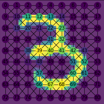
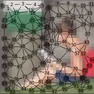
Figure 1. Superpixels for the digit ‘3’ image (left), a boy reading a book (right)

In this work, we leverage spatial information from the image and infuse knowledge in the form of binary relations procured from the superpixel graph representation of the image. CNN filters tend to learn parameters based on pixel-level information. We hypothesise that fusing such superpixel-level information can provide a higher-level understanding of the image and aid a CNN in classification tasks. Specifically, we treat the graph resulting from the image superpixels as an input to a GNN and learn a CNN-based vision system together with the GNN. The coupled hybrid CNN+GNN system is expected to be knowledge-rich, both at the level of raw pixels and superpixels.

Major contributions

Overall, the major contributions of our paper are as follows:

1. Treating the superpixel representation of an image as a graph and allowing a GNN to extract higher-level domain information about an image;

2. We construct an image classification model by coupling the GNN with a CNN-based baseline;

3. We conduct a series of empirical evaluations of our coupled CNN+GNN hybrid system on four different popular image classification benchmarks and three case studies.

The rest of the paper is organised as follows. In Section 2, we provide details of our methodology, including a new loss function suitable for learning the hybrid model. Section 3 provides details of our experiments. Section 4 provides a brief description of related work. Section 5 concludes the paper.

2. Superpixels Integrated Vision Model

2.1. Superpixel Graph Construction

Simple Linear Iterative Clustering (SLIC) (Achanta et al., 2012) is an easy-to-use and straightforward algorithm. SLIC generates superpixels by clustering pixels of an image based on their colour similarity and proximity in the image plane. As a black-box procedure, as is the case in our present study, SLIC takes an approximate number of superpixels and the input image as its input and outputs a segmented image. We use SLIC to construct the segmented version of the input image: each segmented patch in the image is now a superpixel. We then treat the centroid of every superpixel as a node in the graph. We link these nodes by building a radius graph (Bentley et al., 1977). For every pair of nodes, we form an edge between them if and only if the Euclidean distance between them is less than a pre-ordained radius, $r\in\mathbb{R}$. Mathematically, a radius graph is defined as $G=(V,E)$ such that:

$$V =\{x_{i}:x_{i}~{}\text{is a superpixel}\},$$

$$E =\{\{x_{i},x_{j}\}:x_{i,j}\in V,x_{i}\neq x_{j},||x_{i}-_{j}||\leq r\}$$

2.2. The Coupled CNN+GNN Model

Our main motive in this work is to learn jointly from the image and its superpixel representation. This results in a complementary combination of a vision model (CNN) and a relational model (GNN). The CNN takes care of feature extraction (low-level features such as edges in initial layers to complex objects in the latter layers). In contrast, the graph-based model takes the superpixel-based radius graph and extracts relational information about the image that can act as domain knowledge. Fig. 2 illustrates this hybrid combination.

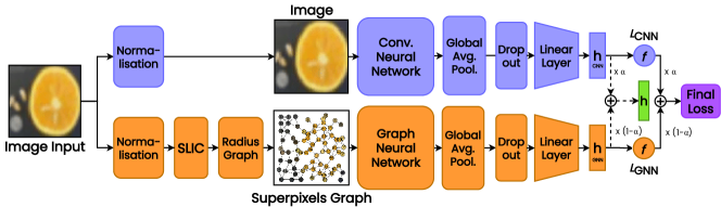
Figure 2. Block diagram of the proposed CNN+GNN model. The hybrid model consists of two backbones: a CNN backbone and a GNN backbone. The input to the CNN backbone is an image, and the input to the GNN backbone is the radius graph (obtained from the superpixel representation) corresponding to the image. The CNN block consists of multiple sub-blocks (layers) of Convolution (C) and Max. Pooling (P) blocks interleaving each other, e.g. CPCPCP. Similarly, there are multiple Graph Convolution blocks (graph attention layers, as in GAT) in the GNN block. The Global Mean Pool blocks read out the final representation from the CNN and GNN. The dropout block (optional) is used to deal with noise in representation and produce a robust representation. $h$ denotes the logits, $\alpha$ is a hyperparameter described later. $\oplus$ is the addition operation.

Regardless of the detailed architectural specifics, the goal is to construct a representation of the input (image) that consists of both the spatial information (extracted by the CNN) and the domain information (extracted by the GNN). This representation can then be used to construct a feedforward fully-connected neural network that outputs a class label for the input image. In order to train the coupled model in an end-to-end fashion and utilise the information from the combined representation adequately, we propose a simple hybrid loss as follows:

(1) $$\mathcal{L}_{CG}=\alpha\mathcal{L}_{C}+(1-\alpha)\mathcal{L}_{G}$$

Here $\mathcal{L}_{C}$ and $\mathcal{L}_{G}$ denote the cross-entropy loss for CNN and GNN, respectively. The parameter $\alpha$ determines the relative importance accorded to the two models during training, i.e., a value $\alpha=0.5$ would mean that both the raw spatial information and the domain information are equally important. For our construction, we treat this as a tunable hyperparameter.

For inference on the trained model (i.e., prediction), we construct hybrid logits based on the logits computed by the CNN backbone and GNN backbone for an input image as follows:

(2) $$\hat{y}=\arg\max_{j}(\alpha h_{C}+(1-\alpha)h_{G})$$

where $h_{C}$ and $h_{G}$ are the logits from CNN and GNN respectively.

3. Empirical Evaluation

3.1. Aims

This study aims to integrate superpixel-level domain knowledge with vision systems, specifically those based on CNNs. Our empirical experiments attempt to answer the following research questions: RQ1: Can GNNs construct rich relational representations from superpixels?; RQ2: Can GNN-constructed knowledge improve CNN-based vision systems?

3.2. Data

We test our hypothesis on a range of datasets: one dataset for handwriting recognition, one from the fashion and clothing domain, two from the object recognition domain, two datasets from the domain of biometrics, and one dataset from the domain of medical diagnosis. We briefly describe these datasets below. A summary of the dataset is provided in Fig. 3 showing the number of classes, number of instances in training and testing set of each dataset.

3.2.1. MNIST

MNIST (LeCun, 1998) is one of the most popular image classification datasets. It is a database of 28x28-sized grayscale images of handwritten digits, and the task is to identify the digit in the image. MNIST has 10 classes, one for every digit.

3.2.2. FMNIST

Fashion-MNIST (FMNIST) (Xiao et al., 2017) is a sister dataset of MNIST, consisting of fashion and clothing items. This dataset was collated from Zalando’s database of article images. Each image is a 28x28 grayscale image. The dataset has 10 classes, one for every fashion article type.

3.2.3. CIFAR-10

CIFAR-10 (Krizhevsky et al., 2010) is an established object recognition dataset, consisting of 32x32 RGB images. It has ten different classes such as aeroplane, automobile, bird, cat, dog. There are 6000 instances for each class.

3.2.4. CIFAR-100

CIFAR-100 (Krizhevsky et al., 2009) is another object recognition dataset, with 100 classes and RGB images, each of size 32x32. This is like the CIFAR-10 dataset, and there are 600 instances for each class.

3.2.5. LFW

The Labelled Faces in the Wild (LFW (Huang et al., 2007b, a)) dataset is a face recognition dataset. Every image is an RGB image of size 250x250. We do not consider all faces in the dataset; we discard faces with less than 20 faces in order to maintain the class balance. After discarding such faces, we have 62 classes.

3.2.6. SOCOFing

The Sokoto Coventry Fingerprint (Shehu et al., 2018) dataset is made up of 6,000 fingerprint images from 600 African subjects. All images are grayscale and have a resolution of 96x103. The task is to identify the person to which the given fingerprint sample belongs.

3.2.7. COVID-19 Radiography

The COVID-19 Radiography Dataset (Chowdhury et al., 2020; Rahman et al., 2021) consists of chest X-ray images for patients with COVID-19, viral pneumonia, lung opacity as well as normal patients, i.e., four classes. Each image is a 299x299 grayscale image. This dataset has been one of the most popular datasets in machine learning studies involving COVID-19 disease.

Dataset	NumClasses	Trainset-size	Testset-size
MNIST	10	60K	10K
FMNIST	10	60K	10K
CIFAR-10	10	50K	10K
CIFAR-100	100	50K	10K
LFW	62	2.4K	0.6K
SOCOFing	600	49K	6K
COVID-19 X-ray	4	19K	2K

Figure 3. Dataset Summary. The sizes shown are the approximate number of instances in the official training set and test set supplied along with each dataset.

3.3. Algorithms and Machines

We use the method described in Sec. 2.1 to construct a superpixel-based radius graph for each image in these datasets. For convenience, we refer to this procedure as $RadiusGraph$ that takes two inputs: a set of images and the number of superpixels ($n$), and returns a set of radius graphs obtained from the superpixel representation of the images.

We use the PyTorch library for the implementation of CNN and PyTorch Geometric for GNN models. We conduct all our experiments on OVHCloud’s “AI Training” platform with the following configurations: 32GB NVIDIA V100S GPU, 45GB main memory, 14 Intel Xeon 2.90GHz processors and a NVIDIA-DGX station with 32GB Tesla V100 GPU,256GB main memory, 40 Intel Xeon 2.20GHz processors.

3.4. Method

Our method is straightforward. For each dataset ($D$), we determine the value of the number of superpixels ($n$) for the procedure $RadiusGraph$ based on visual analysis. Let $D$ be a dataset with a set of images $X$ and their corresponding class-labels $Y$. So, $D$ is written as $(X,Y)$. In the following steps, $D_{tr}$ and $D_{te}$ denote the official train-set and test-set for a dataset $D$. These details can be obtained from the official sources for each dataset as referred in this paper. We outline the steps of our methodology below:

1. Let $X^{\prime}=RadiusGraph(X,n)$

2. $D^{\prime}=(X^{\prime},Y)$

3. Let $D=D_{tr}\cup D_{te}$ and $D^{\prime}=D^{\prime}_{tr}\cup D^{\prime}_{te}$ be the corresponding train-test splits for the image dataset ($D$) and the superpixel graph dataset ($D^{\prime}$)

4. Construct a CNN model using $D_{tr}$: denote as $M_{c}$

5. Construct a coupled CNN+GNN model using $D_{tr}\cup D^{\prime}_{tr}$: denote as $M_{cg}$

6. Let $P_{c}$ be the predictive performance of $M_{c}$ on $D_{te}$

7. Let $P_{cg}$ be the predictive performance of $M_{cg}$ on $D_{te}$

8. Compare $P_{c}$ and $P_{cg}$

The following details pertaining to the above steps are relevant:

• We use $n=75$ for MNIST and FMNIST, $n=100$ for CIFAR, LFW and SOCOFing and $n=200$ for COVID to construct superpixel graphs using $RadiusGraph$; the number of radial neighbours is set to $5$ for MNIST, FMNIST and CIFAR datasets, $27$ for COVID, $10$ for LFW, and $15$ for SOCOFing. This was decided using graph visualisation;

• The node feature-vector for the radius graphs are: the normalised pixel value and the location of centroid in the image, resulting in 3-length feature-vector for MNIST and FMNIST, and 5-length feature-vector for CIFAR, COVID and LFW;

• We use 90:10 split on $D_{tr}$ (correspondingly, $D^{\prime}_{tr}$) to obtain a validation set useful for hyperparameter tuning;

• We use the AdamW optimiser (Loshchilov and Hutter, 2019) for training all our models;

• The hyperparameters are obtained by a sweep across grids such as batch-size: $\{128,256\}$, learning rate: {1e-3,1e-4,1e-5}, weight-decay parameter: $\{0,0.001\}$ for all the datasets;

• CNN structure is built with 3-blocks; each block consists of a convolutional layer, a batch-norm layer, ReLU activation and a max-pool layer. The number of channels in each convolution layer is 32, 64 and 64, respectively;

• The coupled CNN+GNN structure consists of the same CNN backbone as mentioned above; and a GNN structure consisting of three graph-attention layers (GAT) with 32, 64 and 64 channels, respectively, and the number of heads is set to 1;

• To determine the optimal value of $\alpha$, we run a grid search over multiple values in the range $(0,1)$. $\alpha=0.75$ was found to be the optimal value for our datasets. However, as mentioned earlier, it is advised to use $\alpha$ as a trainable hyperparameter for future works.

• We use accuracy as the metric to measure the predictive performance of the models on $D_{te}$.

3.5. Results

In all our experiments, the primary intention is to show whether relational information provided via a superpixel graph is able to aid in improving the performance of a CNN-based model. One should note that the primary backbone of the CNN in the standalone model (CNN) and that in the coupled model remains the same to draw any meaningful conclusion. The principal results of our experiments are reported in Fig. 4. The results demonstrate that the higher-level domain knowledge extracted by a GNN from the superpixel graph is able to substantially boost the predictive performance of CNNs in a hybrid-learning setting in some cases.

Dataset	CNN	CNN+GNN
MNIST	99.30	99.21
FMNIST	91.65	91.50
CIFAR-10	77.80	76.81
CIFAR-100	42.88	46.79
LFW	60.83	66.12
SOCOFing	65.68	93.58
COVID Chest X-ray	89.09	91.01

Figure 4. Predictive performance (Accuracy) of CNN and CNN+GNN on all datasets

Readers familiar with deep neural networks would agree that networks with complex structures and a large number of parameters tend to be more accurate than those with a lesser number of parameters with a simple structure. A valid argument, therefore, could be that our hybrid model has a more complex structure and more number of parameters than a standard CNN model (the baseline in our work), and hence, it could be learning representations for images in a better way than a CNN alone. But, the results presented in this work should be taken with a pinch of salt and should be understood that the GNN in the hybrid model enforces some form of structural constraints to be learned along with the standard convolutions over the input image as is done in CNNs. However, we have made sure that percentage difference in the number of parameters between the two models (CNN and the hybrid) is approximately $10\%$.

4. Related Work

Various graph-based learning approaches for superpixel image classification can be distinguished based on how they perform neighbourhood aggregation. In MoNet (Monti et al., 2017), weighted aggregation is performed by learning a scale factor based on geometric distances. They also test their model on the MNIST Superpixels dataset. In Graph Attention Networks (GATs) (Avelar et al., 2020), self-attention weights are learned. SplineCNN (Fey et al., 2018) uses B-spline bases for aggregation, whereas SGCN (Danel et al., 2020) is a variant of MoNet and uses a different distance metric.

There are some preliminary works on enhancing semantic segmentation based systems using superpixel representations. For instance, Mi et al. (Mi and Chen, 2020) propose a Superpixel-enhanced Region Module (SRM), which they train jointly with a Deep Neural Forest. The SRM alleviates the noise by leveraging the pixel-superpixel associations. In DrsNet (Yu and Fan, 2021), coarse superpixel masking and fine superpixel masking are applied to the CNN features of the input image, particularly for rare classes and background areas. Authors of (Zhao et al., 2017) have used superpixel-based multiple local regions joint representation CNN model to classify very high resolution (VHR) panchromatic and multispectral (MS) remote-sensing images. In (Yang et al., 2021), the authors propose an image recognition method that is based on superpixels and feature fusion, where the features (such as global, texture, appearance features) are computed from the superpixels representation. In (Liu et al., 2019), a superpixel-guided layer-wise embedding CNN is devised by the authors, whose main focus is remote sensing image classification. Superpixels guide the network when it comes to unlabelled samples, and superpixels help in handling irregular spatial dependencies.

5. Conclusion

Our present work demonstrates that superpixels-based graphs represent domain knowledge for images and that infusing this knowledge in a standard vision-based training process shows significant gains in predictive accuracy. We are able to conclude that a GNN can deal with relational information conveyed by a superpixel graph and can construct high-level relations that can boost the predictive performance when coupled with a CNN model. A straightforward extension is to employ a pre-trained CNN model for domain-specific tasks and observe how the superpixel information impacts the predictive performance.

Data and Code Availability

Our code repository is available at: https://github.com/abheesht17/super-pixels. We provide details on how to obtain the data used in our experiments. We also provide details on how to use our code-repository for applications in other domains. The authors can be contacted for more details on the code package.

- (1)
- Achanta et al. (2012) Radhakrishna Achanta, Appu Shaji, Kevin Smith, Aurelien Lucchi, Pascal Fua, and Sabine Süsstrunk. 2012. SLIC superpixels compared to state-of-the-art superpixel methods. IEEE transactions on pattern analysis and machine intelligence 34, 11 (2012), 2274–2282.
- Avelar et al. (2020) Pedro HC Avelar, Anderson R Tavares, Thiago LT da Silveira, Clíudio R Jung, and Luís C Lamb. 2020. Superpixel image classification with graph attention networks. In 2020 33rd SIBGRAPI Conference on Graphics, Patterns and Images (SIBGRAPI). IEEE, 203–209.
- Bentley et al. (1977) Jon L Bentley, Donald F Stanat, and E Hollins Williams Jr. 1977. The complexity of finding fixed-radius near neighbors. Information processing letters 6, 6 (1977), 209–212.
- Chowdhury et al. (2020) Muhammad EH Chowdhury, Tawsifur Rahman, Amith Khandakar, Rashid Mazhar, Muhammad Abdul Kadir, Zaid Bin Mahbub, Khandakar Reajul Islam, Muhammad Salman Khan, Atif Iqbal, Nasser Al Emadi, et al. 2020. Can AI help in screening viral and COVID-19 pneumonia? IEEE Access 8 (2020), 132665–132676.
- Danel et al. (2020) Tomasz Danel, Przemysław Spurek, Jacek Tabor, Marek Śmieja, Łukasz Struski, Agnieszka Słowik, and Łukasz Maziarka. 2020. Spatial graph convolutional networks. In International Conference on Neural Information Processing. Springer, 668–675.
- Dash et al. (2022) Tirtharaj Dash, Sharad Chitlangia, Aditya Ahuja, and Ashwin Srinivasan. 2022. A review of some techniques for inclusion of domain-knowledge into deep neural networks. Scientific Reports 12, 1 (Jan 2022). https://doi.org/10.1038/s41598-021-04590-0
- Dash et al. (2021) Tirtharaj Dash, Ashwin Srinivasan, and Lovekesh Vig. 2021. Incorporating symbolic domain knowledge into graph neural networks. Machine Learning (2021), 1–28.
- Fey et al. (2018) Matthias Fey, Jan Eric Lenssen, Frank Weichert, and Heinrich Müller. 2018. Splinecnn: Fast geometric deep learning with continuous b-spline kernels. In Proceedings of the IEEE Conference on Computer Vision and Pattern Recognition. 869–877.
- Huang et al. (2007a) Gary B Huang, Vidit Jain, and Erik Learned-Miller. 2007a. Unsupervised joint alignment of complex images. In 2007 IEEE 11th international conference on computer vision. IEEE, 1–8.
- Huang et al. (2007b) Gary B. Huang, Manu Ramesh, Tamara Berg, and Erik Learned-Miller. 2007b. Labeled Faces in the Wild: A Database for Studying Face Recognition in Unconstrained Environments. Technical Report 07-49. University of Massachusetts, Amherst.
- Krizhevsky et al. (2009) A Krizhevsky, V Nair, and G Hinton. 2009. CIFAR-100 Dataset (Canadian Institute for Advanced Research).
- Krizhevsky et al. (2010) Alex Krizhevsky, Vinod Nair, and Geoffrey Hinton. 2010. Cifar-10 (Canadian Institute for Advanced Research). URL http://www. cs. toronto. edu/kriz/cifar. html 5 (2010), 4.
- LeCun (1998) Yann LeCun. 1998. The MNIST database of handwritten digits. http://yann. lecun. com/exdb/mnist/ (1998).
- Liu et al. (2019) Han Liu, Jun Li, Lin He, and Yu Wang. 2019. Superpixel-Guided Layer-Wise Embedding CNN for Remote Sensing Image Classification. Remote Sensing 11, 2 (2019). https://doi.org/10.3390/rs11020174
- Loshchilov and Hutter (2019) Ilya Loshchilov and Frank Hutter. 2019. Decoupled Weight Decay Regularization. In International Conference on Learning Representations. https://openreview.net/forum?id=Bkg6RiCqY7
- Mi and Chen (2020) Li Mi and Zhenzhong Chen. 2020. Superpixel-enhanced deep neural forest for remote sensing image semantic segmentation. ISPRS Journal of Photogrammetry and Remote Sensing 159 (2020), 140–152.
- Monti et al. (2017) Federico Monti, Davide Boscaini, Jonathan Masci, Emanuele Rodola, Jan Svoboda, and Michael M Bronstein. 2017. Geometric deep learning on graphs and manifolds using mixture model cnns. In Proceedings of the IEEE conference on computer vision and pattern recognition. 5115–5124.
- Rahman et al. (2021) Tawsifur Rahman, Amith Khandakar, Yazan Qiblawey, Anas Tahir, Serkan Kiranyaz, Saad Bin Abul Kashem, Mohammad Tariqul Islam, Somaya Al Maadeed, Susu M. Zughaier, Muhammad Salman Khan, and Muhammad E.H. Chowdhury. 2021. Exploring the effect of image enhancement techniques on COVID-19 detection using chest X-ray images. Computers in Biology and Medicine 132 (2021), 104319. https://doi.org/10.1016/j.compbiomed.2021.104319
- Ren and Malik (2003) Xiaofeng Ren and Jitendra Malik. 2003. Learning a classification model for segmentation. In Computer Vision, IEEE International Conference on, Vol. 2. IEEE Computer Society, 10–10.
- Scarselli et al. (2008) Franco Scarselli, Marco Gori, Ah Chung Tsoi, Markus Hagenbuchner, and Gabriele Monfardini. 2008. The graph neural network model. IEEE transactions on neural networks 20, 1 (2008), 61–80.
- Shehu et al. (2018) Yahaya Isah Shehu, Ariel Ruiz-Garcia, Vasile Palade, and Anne James. 2018. Sokoto coventry fingerprint dataset. arXiv preprint arXiv:1807.10609 (2018).
- Xiao et al. (2017) Han Xiao, Kashif Rasul, and Roland Vollgraf. 2017. Fashion-mnist: a novel image dataset for benchmarking machine learning algorithms. arXiv preprint arXiv:1708.07747 (2017).
- Yang et al. (2021) Feng Yang, Zheng Ma, and Mei Xie. 2021. Image classification with superpixels and feature fusion method. Journal of Electronic Science and Technology 19, 1 (2021), 100096. https://doi.org/10.1016/j.jnlest.2021.100096 Special Section on In Silico Research on Microbiology and Public Health.
- Yu and Fan (2021) Liangjiang Yu and Guoliang Fan. 2021. DrsNet: Dual-resolution semantic segmentation with rare class-oriented superpixel prior. Multimedia Tools and Applications 80, 2 (2021), 1687–1706.
- Zhao et al. (2017) Wei Zhao, Licheng Jiao, Wenping Ma, Jiaqi Zhao, Jin Zhao, Hongying Liu, Xianghai Cao, and Shuyuan Yang. 2017. Superpixel-based multiple local CNN for panchromatic and multispectral image classification. IEEE Transactions on Geoscience and Remote Sensing 55, 7 (2017), 4141–4156.