Charm-quark mass effects in NRQCD matching coefficients and the leptonic decay of the $\Upsilon(1S)$ meson

Abstract

We compute two-loop corrections to the vector current matching coefficient involving two heavy quark masses. The result is applied to the computation of the $\Upsilon(1S)$ decay width into an electron or muon pair. We complement the next-to-next-to-next-to-leading order corrections of Ref. Beneke:2014qea by charm quark mass effects up to second order in perturbation theory. Furthermore, we apply the formalism to $\Gamma(J/\Psi\to\ell^{+}\ell^{-})$ and compare to the experimental data.

I Introduction

Bottomonia, the bound states of a bottom and an antibottom quark, are excellent systems to investigate the dynamics of bound states in QCD. On the experimental side, there exist precise measurements of their properties. And on the theoretical side, the large mass of the bottom quark means that perturbation theory can be applied. This is in particular the case for the $\Upsilon(1S)$ meson. Nevertheless, its description is complicated by the fact that aside from the bottom-quark mass $m_{b}$ (the hard scale), there are two more relevant scales: the typical momentum and energy of the quarks, which are of order $m_{b}v$ (the soft scale) and $m_{b}v^{2}$ (the ultrasoft scale), respectively. The $\Upsilon(1S)$ is a non-relativistic bound state, where the relative velocity $v$ of the quark and antiquark is small, which means that these scales are well separated. It is then convenient to use an effective theory for the description of this multiscale problem. Starting from QCD, we first integrate out the hard modes to arrive at non-relativistic QCD (NRQCD). In a second step we integrate out the soft modes and potential gluons with ultrasoft energies and soft momenta to arrive at potential NRQCD (PNRQCD). At each step one has to determine the Wilson or matching coefficients of the corresponding effective theory, which are the couplings of the effective operators. For comprehensive reviews on this topic we refer to Pineda:2011dg ; Beneke:2013jia

The main focus of this paper is the matching coefficient $c_{v}$ of the vector current in NRQCD. Among other observables, it contributes to the decay rate of an $\Upsilon(1S)$ to a lepton-antilepton pair. In PNRQCD and to next-to-next-to-next-to-leading order (N³LO) accuracy, the decay rate is given by the formula Beneke:2007gj

$$\Gamma(\Upsilon(1S)\to\ell^{+}\ell^{-}) = \frac{4\pi\alpha^{2}}{9m_{b}^{2}}\left|\psi_{1}(0)\right|^{2}c_{v}\left[c_{v}-\frac{E_{1}}{m_{b}}\left(c_{v}+\frac{d_{v}}{3}\right)+\ldots\right]\,,\quad$$ (1)

where $\alpha$ is the fine structure constant and $m_{b}$ the bottom-quark pole mass. $E_{1}$ and $\psi_{1}(0)$ are the binding energy and the wave function at the origin of the $(b\bar{b})$ system. For convenience we provide the leading order results which are given by

$$\left|\psi_{1}^{\rm LO}(0)\right|^{2}=\frac{8m_{b}^{3}\alpha_{s}^{3}}{27\pi}\,,\quad E_{1}^{\rm LO}=-\frac{4m_{b}\alpha_{s}^{2}}{9}\,.$$ (2)

The matching coefficient $c_{v}$ of the leading current is known at the three-loop level Czarnecki:1997vz ; Beneke:1997jm ; Marquard:2014pea for the case of one massive quark and $n_{l}$ massless quarks. $d_{v}$ is the matching coefficient of the sub-leading $b\bar{b}$ current in NRQCD. Since it is multiplied by $E_{1}$, it is only required at the one-loop level. This result can be found in Ref. Beneke:2013jia . Together with the N³LO results for the energy levels and the wave function at the origin Beneke:2007gj ; Beneke:2007pj ; Beneke:2013jia , this made it possible to evaluate the decay rate at N³LO in Ref. Beneke:2014qea .

One approximation that was made in Ref. Beneke:2014qea was to treat the charm quark as massless. The aim of this paper is to go beyond this approximation and include the corrections due to the charm-quark mass at next-to-next-to-leading order (NNLO). If we consider the charm-quark mass $m_{c}$ to be formally of the order of the hard scale $m_{b}$, the charm quark has to be integrated out of QCD, leading to NRQCD with two heavy quarks with different masses. All NRQCD matching coefficients will then receive contributions due to $m_{c}$. However, at NNLO only $c_{v}$ is affected. Thus we have to compute the fermionic contribution to the two-loop corrections to $c_{v}$ for a second non-zero quark mass. The analytic result for this contribution completes the two-loop evaluation of $c_{v}$ and together with its application to $\Gamma(\Upsilon(1S)\to\ell^{+}\ell^{-})$ constitutes the main result of our paper.

Another possibility to include the charm-quark mass effects is to consider $m_{c}$ to be soft. In this case the charm quark is integrated out of NRQCD. Then there is no contribution to $c_{v}$, but instead to the matching coefficients of PNRQCD, which are the potentials in the Schrödinger equation describing the $(b\bar{b})$ system. At NNLO, only the Coulomb potential is affected (see Section 3.5 of Ref. Beneke:2014pta ). Thus, the $m_{c}$ dependence then enters in the wave function and binding energy. We will compare the results of these two approaches.

The remainder of the paper is organized as follows: In the next section we describe the calculation of $c_{v}$ and in Section III the discussion is extended to external axial-vector, scalar and pseudo-scalar currents, where in addition to the non-singlet also the singlet contributions have to be considered. In Section IV we provide updated predictions for $\Gamma(\Upsilon(1S)\to\ell^{+}\ell^{-})$ and in Section V we consider the decay of the $J/\Psi$ and provide predictions of $\Gamma(J/\Psi\to\ell^{+}\ell^{-})$ up to N³LO. Our conclusions are presented in Section VI. In the Appendix analytic results for all matching coefficients up to two loops, which are not presented in the main part of the paper, are provided. The supplementary material to this paper progdata contains computer-readable expressions of all matching coefficients and all master integrals, which we compute in this paper.

II Two-loop matching coefficient for the vector current with two masses

The matching coefficient for the vector current is defined via

$$j_{v}^{i} = c_{v}\tilde{j}_{v}^{i}+{\cal O}\left(\frac{1}{m_{q}}\right)\,,$$ (3)

where $m_{q}$ is the heavy quark mass and $j_{v}^{i}$ and $\tilde{j}_{v}^{i}$ are currents defined in the full (QCD) and effective (NRQCD) theory. They are given by

$$j_{v}^{\mu} = \bar{\psi}\gamma^{\mu}\psi\,,$$

$$\tilde{j}_{v}^{i} = \phi\sigma^{i}\chi\,,$$ (4)

where $\phi$ and $\chi$ are two-component spinors. Note that in the heavy quark limit the $0^{\rm th}$ component of $j_{v}^{\mu}$ is of order $1/m_{q}^{2}$.

A convenient approach to compute $c_{v}$ is based on the so-called threshold expansion Beneke:1997zp ; Smirnov:2002pj which is applied to the vertex corrections of a vector current and a heavy quark-antiquark pair, $\Gamma_{v}$. Denoting by $Z_{2}$ the on-shell quark wave function renormalization constant one obtains the equation Beneke:1997jm

$$Z_{2}\Gamma_{v}(q_{1},q_{2}) = c_{v}\frac{\tilde{Z}_{2}}{\tilde{Z}_{v}}\tilde{\Gamma}_{v}+{\cal O}\left(\frac{1}{m_{q}}\right)\,.$$ (5)

Note that the vector current in QCD has a vanishing anomalous dimension whereas $\tilde{Z}_{v}$ deviates form 1 at order $\alpha_{s}^{2}$. It gets contributions from the colour factors $C_{F}^{2}$ and $C_{A}C_{F}$ which are not considered in this paper. The momenta $q_{1}$ and $q_{2}$ in Eq. (5) correspond to the outgoing momenta of the quark and antiquark which are considered on-shell. Furthermore, we have $(q_{1}+q_{2})^{2}=4m_{q}^{2}$, a consequence of the threshold expansion.

The quantity $\Gamma_{v}$ is conveniently obtained with the help of projectors applied to the vertex function $\Gamma^{\mu}$. It is straightforward to show that one gets

$$\Gamma_{v} = \mbox{Tr}\left[P^{v}_{\mu}\Gamma^{v,\mu}\right]\,,$$ (6)

with

$$P^{v}_{\mu} = \frac{1}{8(d-1)m_{q}^{2}}\left(-\frac{\not{q}}{2}+m_{q}\right)\gamma_{\mu}\left(\frac{\not{q}}{2}+m_{q}\right)\,,$$ (7)

where $q=q_{1}+q_{2}$.

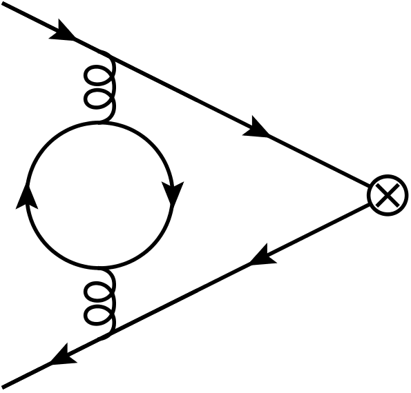
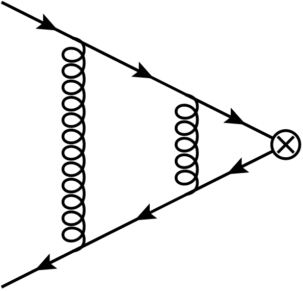
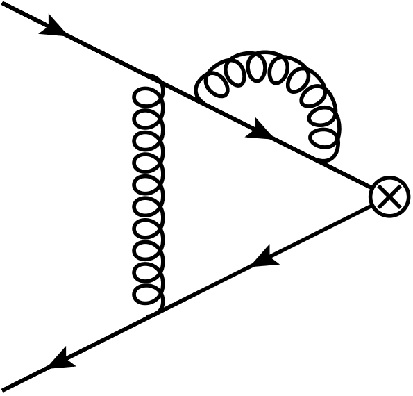
(a)	(b)	(c)	(d)
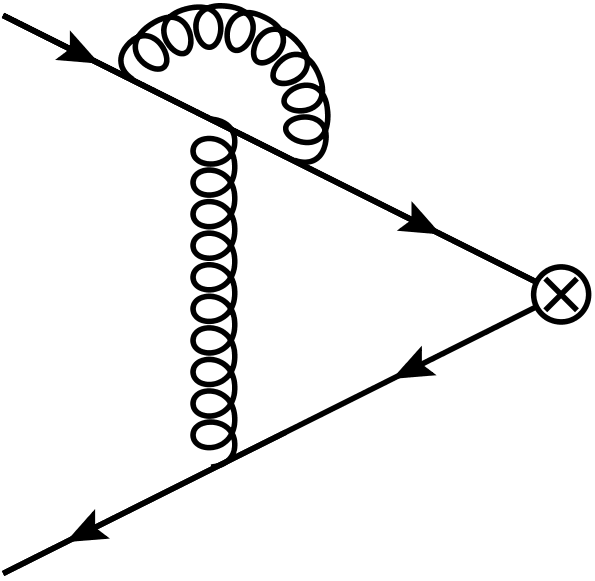
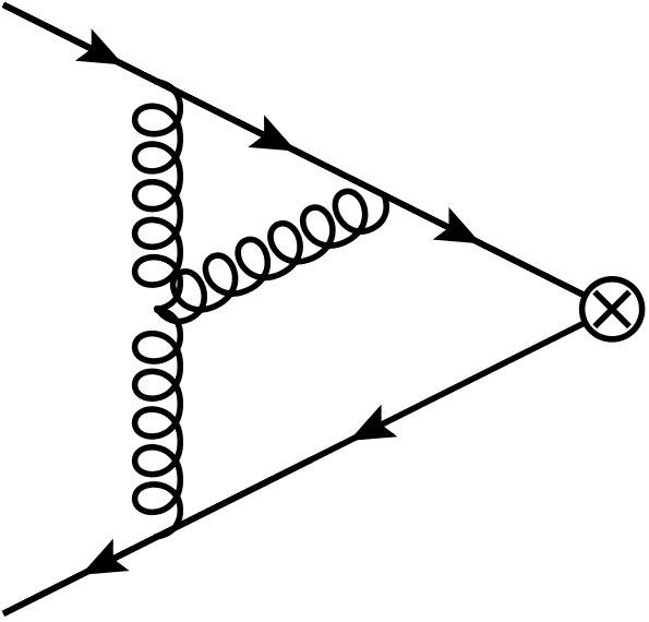
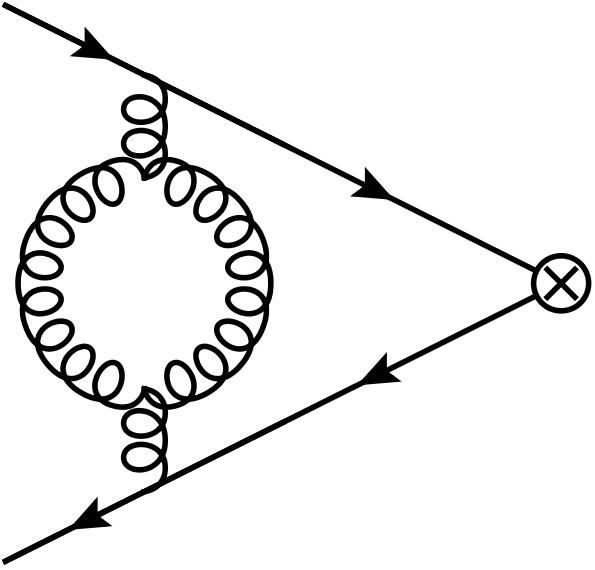
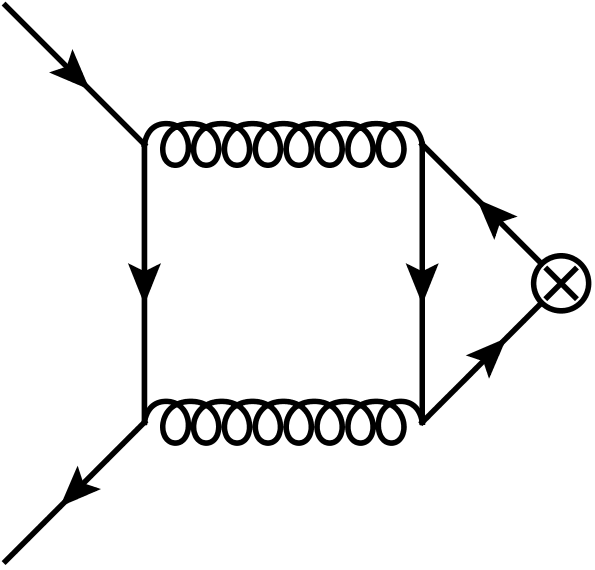
(e)	(f)	(g)	(h)

Figure 1: Sample Feynman diagrams contributions to the matching coefficient $c_{v}$. Straight and curly lines represent quarks and gluons, respectively. The cross represents the external current. The main focus of this paper is diagram (a) where the quark in the closed loop has mass $m_{2}$. Note that the singlet diagram shown in (h) vanishes for an external vector current. However, for an axial-vector, scalar or pseudo-scalar current it is non-zero.

In Fig. 1 we show sample diagrams contributing to $c_{v}$ up to two-loop order. The main focus of this work is the Feynman diagram in Fig. 1(a) where the quark in the closed loop has mass $m_{2}$. For the computation of this diagram we proceed as follows.

• We apply the projector in Eq. (7) to the amplitude of the Feynman diagram in Fig. 1 and take the traces. After decomposing the numerator in terms of denominator factors we obtain scalar integrals of the form

  $$I(n_{1},\ldots,n_{6})=\int\frac{\mathrm{d}^{d}k}{(2\pi)^{d}}\frac{\mathrm{d}^{d}l}{(2\pi)^{d}}\frac{\left(q\cdot l\right)^{-n_{6}}}{\left(-k^{2}\right)^{n_{1}}\left(m_{q}^{2}-\left(\frac{q}{2}+k\right)^{2}\right)^{n_{2}}\left(m_{q}^{2}-\left(-\frac{q}{2}+k\right)^{2}\right)^{n_{3}}\left(m_{2}^{2}-\left(k+l\right)^{2}\right)^{n_{4}}\left(m_{2}^{2}-l^{2}\right)^{n_{5}}}\,.$$

• In a next step we perform a partial fraction decomposition in order to arrive at integral families where the propagator factors are linearly independent. In our case this is achieved with the help of

  $$\int\frac{\mathrm{d}^{d}k}{\left(m_{q}^{2}-\left(\frac{q}{2}+k\right)^{2}\right)\left(m_{q}^{2}-\left(-\frac{q}{2}+k\right)^{2}\right)}=\int\frac{\mathrm{d}^{d}k}{\left(-k^{2}\right)\left(m_{q}^{2}-\left(-\frac{q}{2}+k\right)^{2}\right)}\,.$$ (9)

• We pass the resulting integrals to FIRE Smirnov:2019qkx and LiteRed Lee:2012cn and perform a reduction to four master integrals which are given by

  $$I_{1} = \int\frac{\mathrm{d}^{d}k}{(2\pi)^{d}}\frac{\mathrm{d}^{d}l}{(2\pi)^{d}}\frac{1}{\left(m_{2}^{2}-k^{2}\right)\left(m_{2}^{2}-l^{2}\right)}\,,$$

  $$I_{2} = \int\frac{\mathrm{d}^{d}k}{(2\pi)^{d}}\frac{\mathrm{d}^{d}l}{(2\pi)^{d}}\frac{1}{\left(m_{q}^{2}-k^{2}\right)\left(m_{2}^{2}-l^{2}\right)}\,,$$

  $$I_{3} = \int\frac{\mathrm{d}^{d}k}{(2\pi)^{d}}\frac{\mathrm{d}^{d}l}{(2\pi)^{d}}\frac{1}{\left(m_{q}^{2}-\left(-\frac{q}{2}+k\right)^{2}\right)\left(m_{2}^{2}-\left(k+l\right)^{2}\right)\left(m_{2}^{2}-l^{2}\right)}\,,$$

  $$I_{4} = \int\frac{\mathrm{d}^{d}k}{(2\pi)^{d}}\frac{\mathrm{d}^{d}l}{(2\pi)^{d}}\frac{1}{\left(m_{q}^{2}-\left(-\frac{q}{2}+k\right)^{2}\right)^{2}\left(m_{2}^{2}-\left(k+l\right)^{2}\right)\left(m_{2}^{2}-l^{2}\right)}\,.$$ (10)

  Their graphical representation can be found in Fig. 2.

• Next, we introduce the variable $x=m_{2}/m_{q}$ and establish differential equations for the master integrals of the form

  $$\frac{{\rm d}\vec{I}}{{\rm d}x} = M\cdot\vec{I}\,,$$ (11)

  where the matrix $M$ decomposes into two $1\times 1$ and one $2\times 2$ blocks. The differential equations are brought to $\epsilon$-form using CANONICA Meyer:2017joq :

  $$\frac{{\rm d}\vec{J}}{{\rm d}x} = \epsilon\tilde{M}\cdot\vec{J}\,,$$ (12)

  where the matrix $\tilde{M}$ does not depend on $\epsilon$ and $\vec{I}=T\cdot\vec{J}$. This allows us to compute $\vec{J}$ order-by-order in $\epsilon$ and express the result in terms of iterated integrals which in our case can be expressed in terms of harmonic polylogarithms Remiddi:1999ew .

• In order to fix the boundary conditions we consider the limits $x\to 0$ and $x\to 1$. This is necessary since in each individual limit some of the integration constants drop out. Alternatively it would be possible to solve the differential equation to higher order in $\epsilon$. The values of $\vec{I}$ for $x=0$ and $x=1$ are used to determine the integration constants in $\vec{J}$.

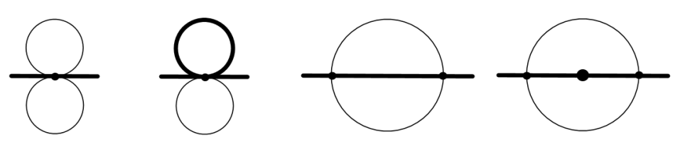
$I_{1}$ $I_{2}$ $I_{3}$ $I_{4}$

Figure 2: Graphical representation of the master integrals of Eq. (10). Thick and thin solid lines represent scalar propagators with mass $m_{q}$ and $m_{2}$, respectively. The external momentum is always $q/2$ with $(q/2)^{2}=m_{q}^{2}$.

We want to remark that we use a general QCD gauge parameter $\xi$ for our computation. The independence of our final result from $\xi$ is a welcome cross check. Our results for the master integrals agree with those given in Appendix B of Ref. Grozin:2020jvt .

For the renormalization of our two-loop contribution we need the two-loop corrections to the on-shell wave-function renormalization constant. The analytic results for the contribution involving $m_{2}$ can be found in Refs. Broadhurst:1991fy ; Bekavac:2007tk ; Davydychev:1998si ; Grozin:2020jvt ; Fael:2020bgs . Furthermore the one-loop counterterm for $\alpha_{s}$ is needed. At this point we use Eq. (5) in order to extract $c_{v}$.

For the fermionic contributions to $c_{v}$ it is convenient to introduce $n_{f}=n_{h}+n_{m}+n_{l}$, where $n_{h}=1$ and $n_{m}=1$ label the contributions with closed massive quark loops with mass $m_{q}$ and $m_{2}$, respectively. $n_{l}$ counts the massless quarks. Using this notation we can cast the result for $c_{v}$ in the form

$$c_{v} = 1-2C_{F}\frac{\alpha_{s}^{(n_{l}+n_{m})}(\mu)}{\pi}+\left(\frac{\alpha_{s}^{(n_{l}+n_{m})}(\mu)}{\pi}\right)^{2}c_{v}^{(2)}+{\cal O}(\alpha_{s}^{3})$$ (13)

where $\alpha_{s}^{(n_{l}+n_{m})}(\mu)$ is the strong coupling constant where the heavy quark with mass $m_{q}$ is decoupled from the running of $\alpha_{s}$. The $m_{2}$-independent contributions to $c_{v}^{(2)}$ can be found in Refs. Czarnecki:1997vz ; Beneke:1997jm ; Kniehl:2006qw . The new contribution proportional to $n_{m}$ reads

$$c_{v}^{(2)}\Big{|}_{m_{2}} = n_{m}C_{F}T_{F}\Bigg{[}\frac{71}{72}+\frac{35x^{2}}{24}+\pi^{2}\bigg{(}\frac{3}{32x}-\frac{11x}{48}-\frac{17x^{3}}{32}+\frac{2x^{4}}{9}\bigg{)}+\frac{1}{24}\big{(}23+19x^{2}\big{)}H_{0}+\frac{4}{3}x^{4}H_{0}^{2}$$ (14)

$$\mbox{}+\bigg{(}\frac{3}{16x}-\frac{11x}{24}-\frac{17x^{3}}{16}+\frac{4x^{4}}{3}\bigg{)}H_{0}H_{1}+\bigg{(}-\frac{3}{16x}+\frac{11x}{24}+\frac{17x^{3}}{16}-\frac{4x^{4}}{3}\bigg{)}H_{0,1}$$

$$\mbox{}+\bigg{(}\frac{3}{16x}-\frac{11x}{24}-\frac{17x^{3}}{16}-\frac{4x^{4}}{3}\bigg{)}H_{-1,0}+\frac{2}{3}\log\bigg{(}\frac{\mu^{2}}{m_{2}^{2}}\bigg{)}\Bigg{]}\,,$$

where $H_{i\ldots}=H_{i\ldots}(x)$ and $H_{i\ldots}(x)$ are harmonic polylogarithms (HPLs) Remiddi:1999ew . Note that for $x\to 1$ we reproduce the known result for $m_{2}=m_{q}$ which is given by

$$c_{v}^{(2)}\Big{|}_{m_{2}} \stackrel{{\scriptstyle x\to 1}}{{\longrightarrow}} C_{F}T_{F}\left(\frac{22}{9}-\frac{2}{9}\pi^{2}+\frac{2}{3}\log\left(\frac{\mu^{2}}{m_{q}^{2}}\right)\right)\,.$$ (15)

However, in the limit $x\to 0$ we do not obtain the massless fermion contribution but recover the well-known Coulomb singularity, which is regulated by the mass $m_{2}$. For small $m_{2}$ we have

$$c_{v}^{(2)}\Big{|}_{m_{2}} \stackrel{{\scriptstyle x\to 0}}{{\longrightarrow}} C_{F}T_{F}\left(\frac{3\pi^{2}}{32x}+{\frac{11}{18}}+\frac{2}{3}\log\left(\frac{\mu^{2}}{m_{q}^{2}}\right)+{\cal O}(x)\right)\,.$$ (16)

In the application we discuss in Section IV we need $c_{v}$ expressed in term of $\alpha_{s}^{(nl=3)}$ which means that we have to decouple the charm quark from the running of $\alpha_{s}$. As a consequence $\mu^{2}$ is effectively replaced by $m_{2}^{2}$ in Eqs. (14), (15) and (16) disappear.

Let us finally investigate the numerical effect of the new contribution. We specify to the bottom-charm system and use $m_{2}=m_{c}=1.65$ GeV and $m_{q}=m_{b}=5.1$ GeV for the pole masses of the charm and bottom quarks. This leads to

$$c_{v}^{(2)}=-44.72+0.17n_{h}+0.41n_{l}+1.75n_{m}+\log\left(\frac{\mu^{2}}{m_{q}^{2}}\right)\left[-20.13+0.44(n_{l}+n_{m})\right],$$ (17)

where the contributions originating from the closed massless, bottom and charm quark loops are marked by $n_{l}=3$, $n_{h}=1$ and $n_{m}=1$, respectively. One observes that the coefficient of $n_{m}$ is more than a factor four times larger than the coefficients of $n_{l}$ and $n_{h}$. Thus, the contribution of the heavy quark with mass $m_{2}$ is larger than the contributions of the heavy quark with mass $m_{q}$ and all three massless quarks combined.

III Two-loop two-mass matching coefficients for axial-vector, scalar and pseudo-scalar currents.

In this Section we consider further external currents, which are of phenomenological relevance, and compute the corresponding matching coefficients between QCD and NRQCD to two-loop order. Such currents have, in contrast to the vector case, both non-singlet and singlet contributions. The latter are characterized by the fact that the external current does not directly couple to the quarks in the final state but only through the exchange of two gluons. A sample Feynman diagram is shown in Fig. 1(h).

We write the two-loop corrections in the form

$$c_{x}^{(2)}=c^{(2)}_{x,\rm non-sing}+c^{(2)}_{x,\rm sing}\,,$$ (18)

where $x\in\{a,s,p\}$ stands for an axial-vector, scalar or pseudo-scalar. All two-loop corrections which involve only one mass scale have been computed in Ref. Kniehl:2006qw . In this paper we concentrate on the diagrams where a second massive quark in a closed loop is present which concerns both the non-singlet and the singlet contribution.

In analogy to Eq. (3) we define the additional currents in QCD via

$$j_{a}^{\mu} = \bar{\psi}\gamma^{\mu}\gamma_{5}\psi\,,$$

$$j_{s} = \bar{\psi}\psi\,,$$

$$j_{p} = \bar{\psi}i\gamma_{5}\psi\,.$$ (19)

The anomalous dimension of $j_{a}^{\mu}$ is zero. For the scalar and pseudo-scalar current we have for the corresponding renormalization constant $Z_{s}=Z_{p}=Z_{m}$, where $Z_{m}$ is the (on-shell) mass renormalization constant.

In NRQCD the currents read Kniehl:2006qw

$$\tilde{j}_{a}^{i} = \frac{1}{2m}\phi^{\dagger}[\sigma^{i},\vec{p}\cdot\vec{\sigma}]\chi\,,$$

$$\tilde{j}_{s} = -\frac{1}{m}\phi^{\dagger}\vec{p}\cdot\vec{\sigma}\chi\,,$$

$$\tilde{j}_{p} = -i\phi^{\dagger}\chi\,,$$ (20)

where $k=1,2,3$. Furthermore we have $j_{a}^{0}=i\tilde{j}_{p}$ which constitutes an alternative way to compute the matching coefficient $c_{p}$. Note the presence of the momentum $\vec{p}$, which is the relative momentum of the external quark and antiquark, in the definition of the axial-vector and scalar current. Thus, an expansion in $p$ has to be performed in order to obtain the loop corrections to the corresponding matching coefficients.

The matching equation in (5) also holds for the other currents after the obvious replacements of $\Gamma_{v}$, $\tilde{Z}_{v}$ and $\tilde{\Gamma}_{v}$.

For the pseudo-scalar current and the zero component of the axial-vector the momentum $p$ is zero and the calculation proceeds in close analogy to the vector case. In fact, we have Kniehl:2006qw .

$$\Gamma_{p} = \mbox{Tr}\left[P^{(p)}\Gamma^{(p)}\right]\,,$$

$$\Gamma_{a,0} = \mbox{Tr}\left[P^{(a,0)}_{\mu}\Gamma^{(a),\mu}\right]\,,$$ (21)

with

$$P^{(p)} = \frac{1}{8m_{q}^{2}}\left(-\frac{\not{q}}{2}+m_{q}\right)\gamma_{5}\left(\frac{\not{q}}{2}+m_{q}\right)\,,$$

$$P^{(a,0)}_{\mu} = -\frac{1}{8m_{q}^{2}}\left(-\frac{\not{q}}{2}+m_{q}\right)\gamma_{\mu}\gamma_{5}\left(\frac{\not{q}}{2}+m_{q}\right)\,.$$ (22)

For the axial-vector and scalar cases there are similar equations to Eq. (21). The expansion in $p$ (up to linear order) is conveniently realized by choosing $q_{1}=q/2+p$ and $q_{2}=q/2-p$, which implies $q\cdot p=0$. Thus the projectors are more complicated and are given by

$$P_{(a,i),\mu} = -\frac{1}{8m_{q}^{2}}\left\{\frac{1}{d-1}\left(-\frac{\not{q}}{2}+m_{q}\right)\gamma_{\mu}\gamma_{5}\left(-\frac{\not{q}}{2}+m_{q}\right)\right.$$

$$\left.-\frac{1}{d-2}\left(-\frac{\not{q}}{2}+m\right)\frac{m}{p^{2}}\left((d-3)p_{\mu}+\gamma_{\mu}\not{p}\right)\gamma_{5}\left(\frac{\not{q}}{2}+m\right)\right\}\,,$$

$$P_{(s)} = \frac{1}{8m_{q}^{2}}\left\{\left(-\frac{\not{q}}{2}+m\right){\bf 1}\left(-\frac{\not{q}}{2}+m\right)+\left(-\frac{\not{q}}{2}+m\right)\frac{m}{p^{2}}\not{p}\left(\frac{\not{q}}{2}+m\right)\right\}\,.$$ (23)

After the application of the projectors and the expansion in $p$ we can set $p=0$ and $q^{2}=4m_{q}^{2}$.

The calculation of the non-singlet contribution is in close analogy to the vector case, see Section II. In particular, it is possible to use anticommuting $\gamma_{5}$. Furthermore, we can map the scalar integrals contributing to $\Gamma_{x}$ after the application of the projector to the same integral families and we thus end up with the same master integrals.

The singlet contribution is more involved and a few comments are in order. Let us first mention that a non-zero contribution for the scalar and pseudo-scalar currents is only obtained for massive quarks in the closed fermion loop. Furthermore, for the axial-vector current an effective current formed by the difference of the upper and lower component of a given quark doublet should be considered in order to guarantee the cancellation of anomaly-like contributions. For example, for the top-bottom doublet we have

$$j_{a}^{\mu} = \bar{t}\gamma^{\mu}\gamma_{5}t-\bar{b}\gamma^{\mu}\gamma_{5}b\,.$$ (24)

In practice, this means that we have a quark with mass $m_{q}$ in the final state and we consider both a massless quark and a quark with mass $m_{2}$ in the closed quark loop and take the difference.

In the singlet diagrams we treat $\gamma_{5}$ according to the prescription of Ref. Larin:1993tq . In the Feynman diagrams we apply for the axial-vector and pseudo-scalar couplings the replacements

$$\gamma^{\mu}\gamma_{5} \to \frac{i}{3!}\varepsilon^{\mu\nu\rho\sigma}\gamma_{\nu}\gamma_{\rho}\gamma_{\sigma}\,,$$

$$\gamma_{5} \to \frac{i}{4!}\varepsilon^{\mu\nu\rho\sigma}\gamma_{\mu}\gamma_{\nu}\gamma_{\rho}\gamma_{\sigma}\,.$$ (25)

We perform the same substitution also in the corresponding projectors. Afterwards we strip off the two $\varepsilon$ tensors and interpret the product in $d$ dimensions. This allows us to perform the calculation in close analogy to the scalar current.

The remaining calculation of the singlet diagrams proceeds as outlined in the previous section. After applying a partial fraction decomposition, we can map all integrals in our amplitude to two integral families which are given by

$$J_{1}(\vec{n}) =\int\frac{{\rm d}^{d}k}{(2\pi)^{d}}\frac{{\rm d}^{d}l}{(2\pi)^{d}}\frac{1}{\left(m_{2}^{2}-(k+\tfrac{q}{2})^{2}\right)^{n_{1}}\left(m_{2}^{2}-(k-\tfrac{q}{2})^{2}\right)^{n_{2}}\left(m_{2}^{2}-(k-l)^{2}\right)^{n_{3}}\left(m_{q}^{2}-l^{2}\right)^{n_{4}}\left(-(l+\tfrac{q}{2})^{2}\right)^{n_{5}}}~{},$$ (26)

$$J_{2}(\vec{n}) =\int\frac{{\rm d}^{d}k}{(2\pi)^{d}}\frac{{\rm d}^{d}l}{(2\pi)^{d}}\frac{1}{\left(m_{2}^{2}-(k+\tfrac{q}{2})^{2}\right)^{n_{1}}\left(m_{2}^{2}-(k-\tfrac{q}{2})^{2}\right)^{n_{2}}\left(m_{2}^{2}-(k-l)^{2}\right)^{n_{3}}\left(-(l+\tfrac{q}{2})^{2}\right)^{n_{4}}\left(-(l-\tfrac{q}{2})^{2}\right)^{n_{5}}}~{}.$$ (27)

The reduction to master integrals using FIRE Smirnov:2019qkx and LiteRed Lee:2012cn leads to 12 master integrals which are shown in Fig. 3. In a next step we establish differential equations in the variable $t$ defined by $x=2t/(1+t^{2})$. In this new variable the differential equation can be brought into $\epsilon$-form with the help of CANONICA Meyer:2017joq . We expand the solution including terms of order $\epsilon$ since some of the master integrals have $1/\epsilon$ poles in the prefactor. The differential equations are integrated with the help of HarmonicSums HarmonicSums in terms of cyclotomic harmonic polylogarithms over the alphabet

$$f_{0}(\tau) =\frac{1}{\tau}, f_{1}(\tau) =\frac{1}{1-\tau}, f_{-1}(\tau) =\frac{1}{1+\tau}, f_{\{4,1\}}(\tau) =\frac{\tau}{1+\tau^{2}}.$$ (28)

Alternatively one could factorize the denominators over the complex numbers and arrive at Goncharov polylogarithms. The boundary conditions are obtained from the single-scale master integrals needed for the two-loop calculation of Refs. Kniehl:2006qw ; Piclum:2007an . For the master integrals with dots the naive $m_{2}=0$ limit is not enough and we have to consider the asymptotic expansion around $m_{2}=0$ which can be obtained easily from one-dimensional Mellin-Barnes representations or a diagrammatic large momentum expansion of the corresponding Feynman integrals. In a second approach we use the algorithm described in Ablinger:2018zwz to solve the differential equations in the variable $x$ without going into an $\epsilon$-form first. For the implementation we additionally make use of Sigma Schneider:2007 and OreSys ORESYS . This approach introduces the square-root valued letter $\sqrt{1-\tau^{2}}/\tau$. Both results agree after the above mentioned variable transformation. We compute the $\epsilon$ expansion of all master integrals up to the order which is needed to obtain the ${\cal O}(\epsilon)$ terms of the matching coefficients.

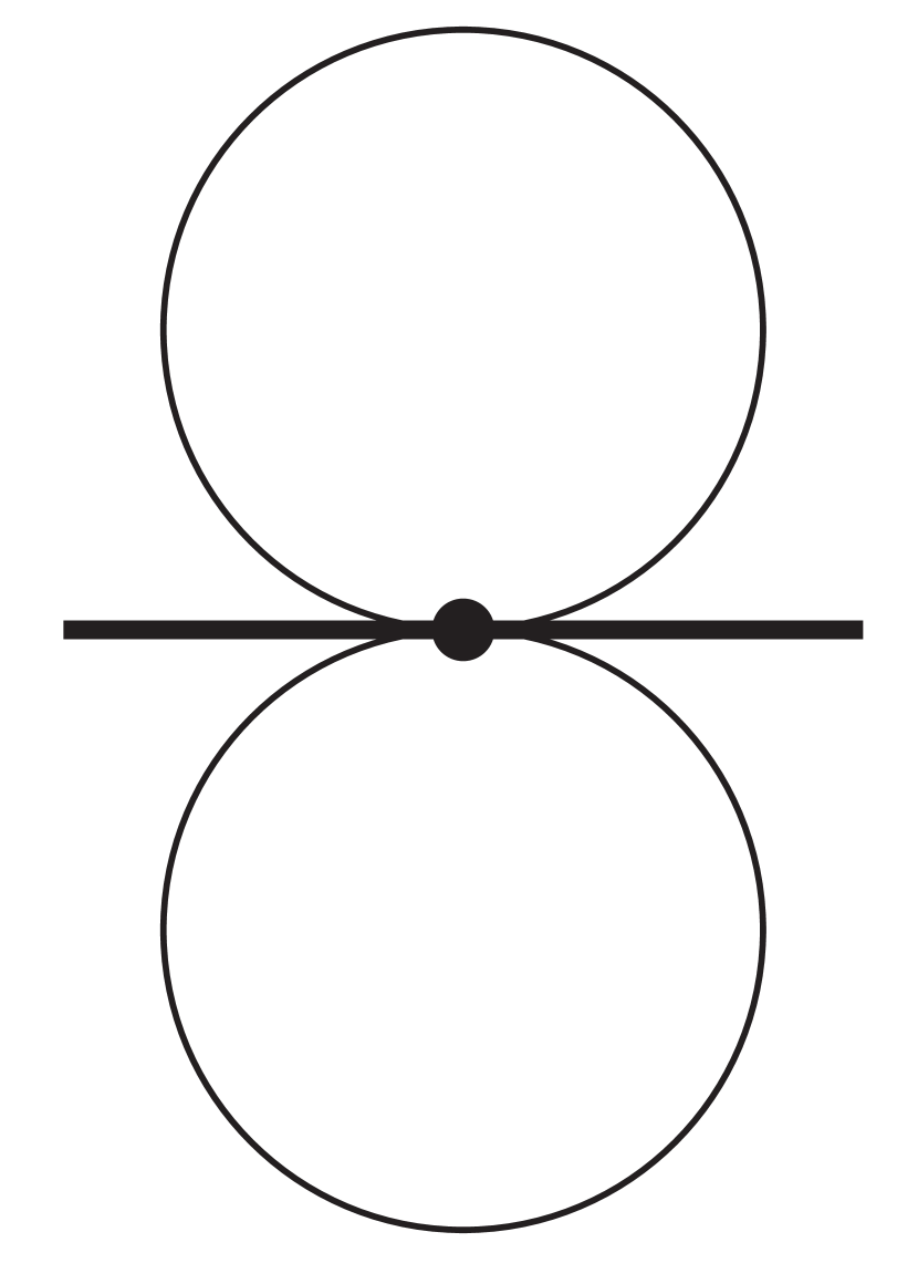
$S_{1}=J_{1}(0,1,1,0,0)$

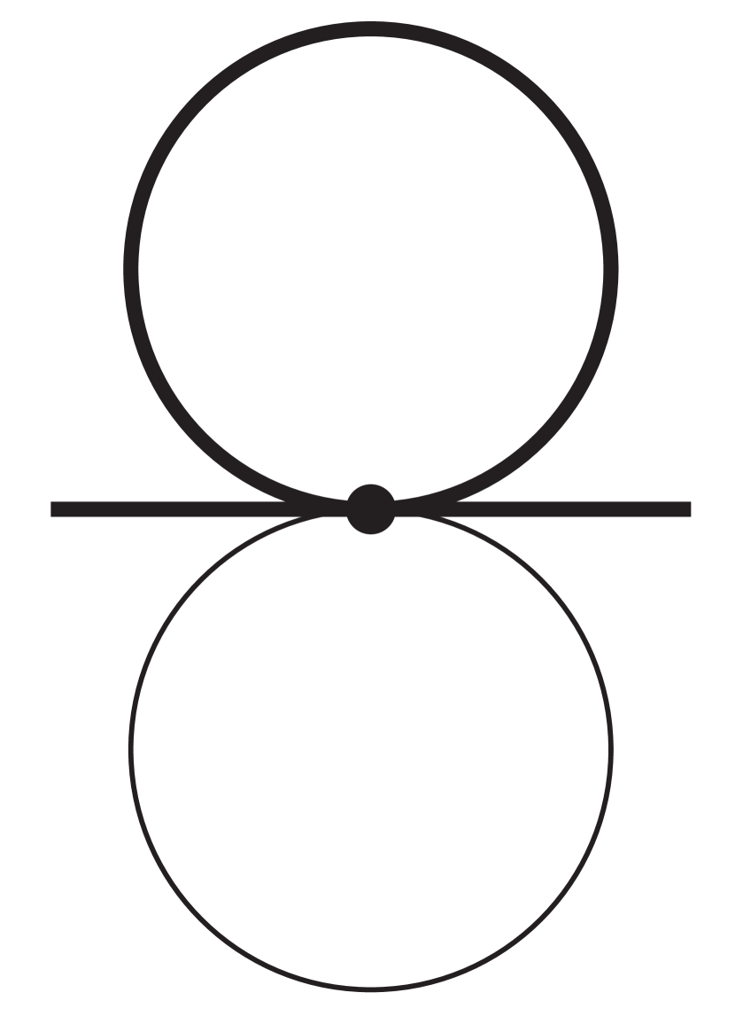
$S_{2}=J_{1}(0,0,1,1,0)$

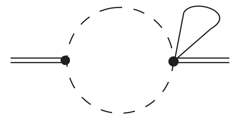
$S_{3}=J_{2}(0,0,1,1,1)$

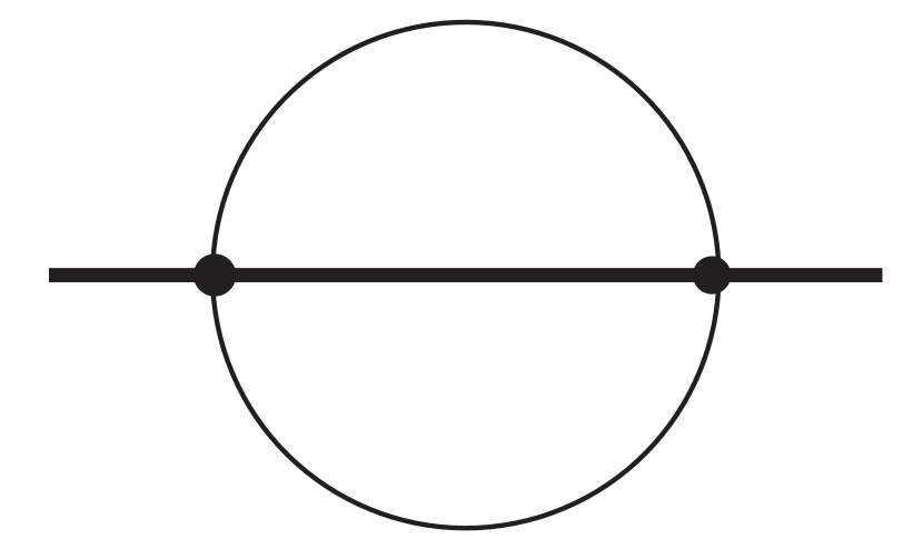
$S_{4}=J_{1}(0,1,1,1,0)$

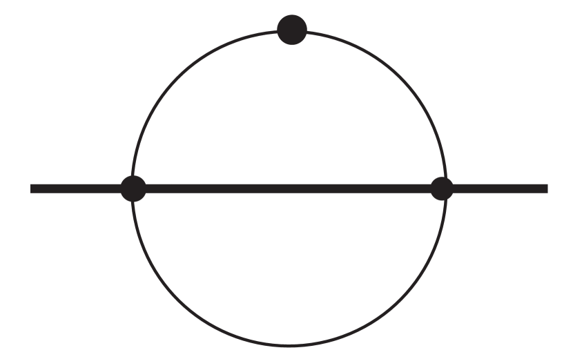
$S_{5}=J_{1}(0,2,1,1,0)$

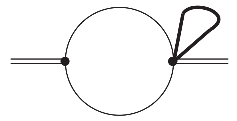
$S_{6}=J_{1}(1,1,0,1,0)$

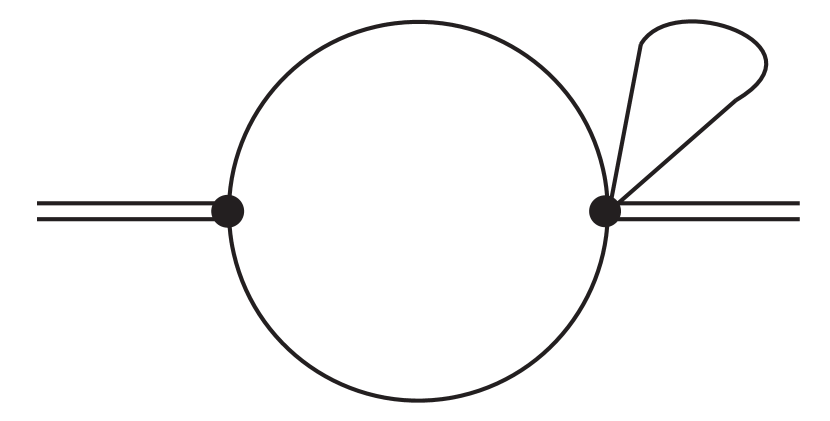
$S_{7}=J_{1}(1,1,1,0,0)$

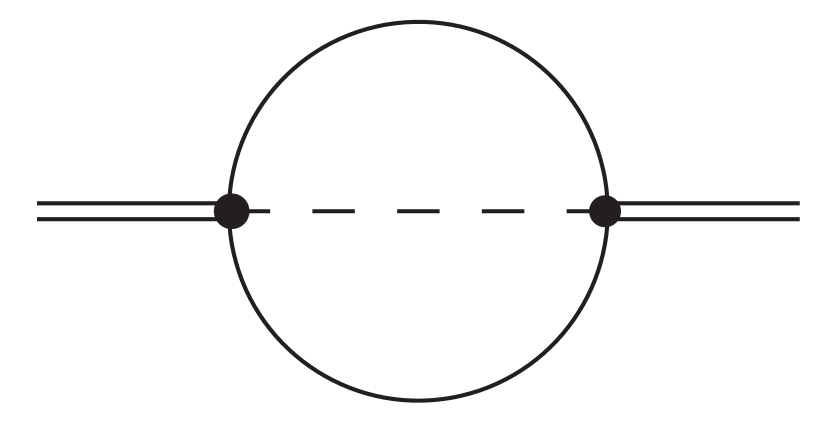
$S_{8}=J_{1}(0,1,1,0,1)$

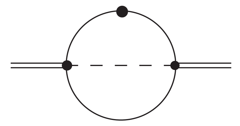
$S_{9}=J_{1}(0,2,1,0,1)$

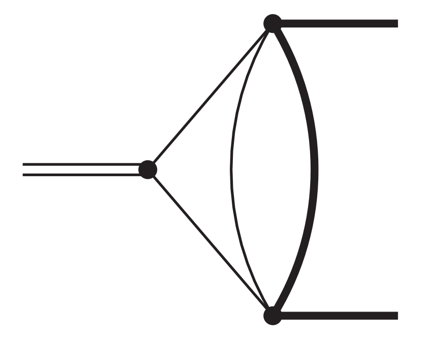
$S_{10}=J_{1}(1,1,1,1,0)$

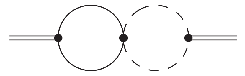
$S_{11}=J_{2}(1,1,0,1,1)$

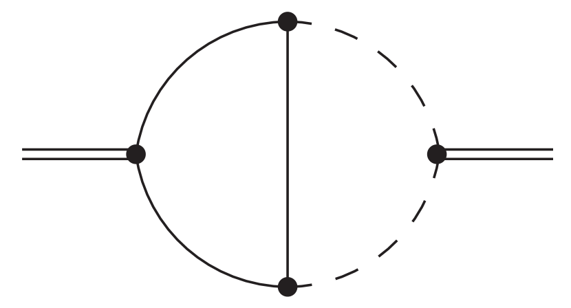
$S_{12}=J_{2}(1,1,1,1,1)$

Figure 3: Master integrals needed for the calculation of the singlet diagrams. Thick and thin lines represent scalar propagators with mass $m_{q}$ and $m_{2}$, respectively. Dashed lines represent massless scalar propagators. External double lines represent the momentum $q$ and thick lines the momentum $q/2$ with $q^{2}=4m_{q}^{2}$.

After inserting the master integrals into the integration-by-parts-reduced amplitude we obtain for the two-loop singlet contribution to the matching coefficient of the scalar current the following expression

$$c_{s,\rm sing}^{(2)}\Big{|}_{m_{2}} =n_{m}C_{F}T_{F}\Biggl{[}\frac{4t}{3\big{(}1+t^{2}\big{)}}+\pi^{2}\biggl{[}\frac{t\big{(}1-28t^{2}-35t^{4}\big{)}}{18\big{(}1+t^{2}\big{)}^{3}}+\frac{4t^{3}H_{1}}{3\big{(}1+t^{2}\big{)}^{3}}+\frac{2t\big{(}3+2t^{2}+3t^{4}\big{)}H_{\{4,1\}}}{3\big{(}1+t^{2}\big{)}^{3}}+\frac{4t^{3}H_{-1}}{\big{(}1+t^{2}\big{)}^{3}}\biggr{]}$$

$$+\log(2)\biggl{[}-\frac{8t^{3}H_{0}}{3\big{(}1+t^{2}\big{)}^{2}}+\biggl{(}-\frac{4t}{3\big{(}1+t^{2}\big{)}}+\frac{32t^{3}H_{-1}}{3\big{(}1+t^{2}\big{)}^{3}}\biggr{)}H_{1}+\frac{16t^{3}H_{1}^{2}}{3\big{(}1+t^{2}\big{)}^{3}}+\frac{4tH_{-1}}{3\big{(}1+t^{2}\big{)}}+\frac{16t^{3}H_{-1}^{2}}{3\big{(}1+t^{2}\big{)}^{3}}\biggr{]}$$

$$+\frac{4t^{3}H_{0}}{\big{(}1+t^{2}\big{)}^{2}}+\frac{4t^{3}\big{(}3+4t^{2}\big{)}H_{0}^{2}}{3\big{(}1+t^{2}\big{)}^{3}}+\biggl{(}\frac{4t\big{(}3t^{2}-5\big{)}H_{0}}{3\big{(}1+t^{2}\big{)}^{2}}+\frac{16t^{3}H_{0}^{2}}{3\big{(}1+t^{2}\big{)}^{3}}\biggr{)}H_{1}+\frac{16t^{3}H_{0}H_{1}^{2}}{3\big{(}1+t^{2}\big{)}^{3}}$$

$$+\biggl{(}-\frac{4t}{1+t^{2}}+\frac{8t(1-t^{2})H_{0}}{3\big{(}1+t^{2}\big{)}^{2}}-\frac{8t\big{(}3+2t^{2}+3t^{4}\big{)}H_{0}^{2}}{3\big{(}1+t^{2}\big{)}^{3}}\biggr{)}H_{\{4,1\}}+\biggl{(}\frac{4t\big{(}5-3t^{2}\big{)}}{3\big{(}1+t^{2}\big{)}^{2}}-\frac{32t^{3}H_{0}}{\big{(}1+t^{2}\big{)}^{3}}$$

$$-\frac{32t^{3}H_{1}}{3\big{(}1+t^{2}\big{)}^{3}}\biggr{)}H_{0,1}+\biggl{(}\frac{8t\big{(}3t^{2}-1\big{)}}{3\big{(}1+t^{2}\big{)}^{2}}+\frac{8t\big{(}3+2t^{2}+3t^{4}\big{)}H_{0}}{\big{(}1+t^{2}\big{)}^{3}}\biggr{)}H_{0,\{4,1\}}+\frac{8tH_{1,\{4,1\}}}{3\big{(}1+t^{2}\big{)}}$$

$$+\biggl{(}\frac{4t\big{(}5-3t^{2}\big{)}}{3\big{(}1+t^{2}\big{)}^{2}}+\frac{64t^{3}H_{0}}{3\big{(}1+t^{2}\big{)}^{3}}+\frac{32t^{3}H_{1}}{3\big{(}1+t^{2}\big{)}^{3}}\biggr{)}H_{-1,0}-\biggl{(}\frac{8t}{3\big{(}1+t^{2}\big{)}}+\frac{64t^{3}H_{1}}{3\big{(}1+t^{2}\big{)}^{3}}\biggr{)}H_{-1,\{4,1\}}$$

$$+\frac{160t^{3}H_{0,0,1}}{3\big{(}1+t^{2}\big{)}^{3}}-\frac{8t\big{(}3-2t+3t^{2}\big{)}\big{(}3+2t+3t^{2}\big{)}H_{0,0,\{4,1\}}}{3\big{(}1+t^{2}\big{)}^{3}}+\frac{32t^{3}H_{0,1,1}}{3\big{(}1+t^{2}\big{)}^{3}}-\frac{64t^{3}H_{1,1,\{4,1\}}}{3\big{(}1+t^{2}\big{)}^{3}}$$

$$-\frac{160t^{3}H_{-1,0,0}}{3\big{(}1+t^{2}\big{)}^{3}}-\frac{32t^{3}H_{-1,0,1}}{3\big{(}1+t^{2}\big{)}^{3}}+\frac{64t^{3}H_{-1,\{4,1\},1}}{3\big{(}1+t^{2}\big{)}^{3}}+\frac{32t^{3}H_{-1,-1,0}}{3\big{(}1+t^{2}\big{)}^{3}}-\frac{64t^{3}H_{-1,-1,\{4,1\}}}{3\big{(}1+t^{2}\big{)}^{3}}$$

$$-\frac{2t\log^{2}(2)}{3\big{(}1+t^{2}\big{)}}-\frac{t\big{(}3+4t^{2}+3t^{4}\big{)}\zeta(3)}{\big{(}1+t^{2}\big{)}^{3}}$$

$$+i\pi\Biggl{\{}\frac{2\pi^{2}t^{3}}{3\big{(}1+t^{2}\big{)}^{3}}+\frac{2t^{3}}{\big{(}1+t^{2}\big{)}^{2}}+\biggl{(}\frac{4t^{3}\big{(}4+5t^{2}\big{)}}{3\big{(}1+t^{2}\big{)}^{3}}+\frac{32t^{3}H_{-1}}{3\big{(}1+t^{2}\big{)}^{3}}\biggr{)}H_{0}$$

$$-\biggl{(}\frac{8t(1-t^{2})}{3\big{(}1+t^{2}\big{)}^{2}}-\frac{16t^{3}H_{0}}{3\big{(}1+t^{2}\big{)}^{3}}\biggr{)}H_{1}+\biggl{(}\frac{4t(1-t^{2})}{3\big{(}1+t^{2}\big{)}^{2}}-\frac{8t\big{(}3+2t^{2}+3t^{4}\big{)}H_{0}}{3\big{(}1+t^{2}\big{)}^{3}}\biggr{)}H_{\{4,1\}}$$

$$+\frac{8t(1-t^{2})H_{-1}}{3\big{(}1+t^{2}\big{)}^{2}}-\frac{16t^{3}H_{0,1}}{\big{(}1+t^{2}\big{)}^{3}}+\frac{4t\big{(}3+2t^{2}+3t^{4}\big{)}H_{0,\{4,1\}}}{\big{(}1+t^{2}\big{)}^{3}}-\frac{16t^{3}H_{-1,0}}{\big{(}1+t^{2}\big{)}^{3}}+\frac{2t(1-t^{2})\log(2)}{3\big{(}1+t^{2}\big{)}^{2}}\Biggr{\}}\Biggr{]}\,,$$ (29)

with $t=(1-\sqrt{1-x^{2}})/x$ and $H_{\vec{a}}=H_{\vec{a}}(t)$. The imaginary part of the matching coefficient is displayed in the last three lines of Eq. (29). For the expansions around $x=0$ we find

$$c_{s,sing}^{(2)}\Big{|}_{m_{2},x\to 0} =n_{m}C_{F}T_{F}\biggr{[}x\biggl{(}\frac{2}{3}+\frac{\pi^{2}}{36}-\frac{\log^{2}(2)}{3}-\frac{3\zeta(3)}{2}\biggr{)}+x^{3}\biggl{(}-\frac{7}{24}-\frac{\pi^{2}}{12}+\frac{7}{12}\log(x)-\frac{3\log(2)}{4}-\frac{1}{3}\log(2)\log(x)$$

$$+\frac{\log^{2}(2)}{3}+\frac{\zeta(3)}{4}\biggr{)}+i\pi\biggl{\{}\frac{1}{3}x\log(2)+x^{3}\biggl{(}\frac{3}{8}+\frac{\pi^{2}}{12}+\frac{1}{6}\log(x)-\frac{\log(2)}{3}\biggr{)}\biggr{\}}+\mathcal{O}(x^{4})\biggr{]}\,.$$ (30)

As expected, this contribution to the matching coefficient is zero for vanishing quark mass in the closed triangle. Note that mass corrections are linear in $m_{2}$. On the other hand, for $x\to 1$ $c_{s,sing}^{(2)}\Big{|}_{m_{2}}$ approaches a constant. Higher order expansion terms are conveniently expressed in terms of $y=1-x$ and are given by

$$c_{s,sing}^{(2)}\Big{|}_{m_{2},x\to 1} =n_{m}C_{F}T_{F}\biggl{[}\frac{2}{3}-\frac{29\pi^{2}}{72}-\log(2)+\frac{2}{3}\pi^{2}\log(2)+y\biggl{(}-\frac{2}{3}+\frac{53\pi^{2}}{72}+\log(2)-\pi^{2}\log(2)-\frac{21\zeta(3)}{4}\biggr{)}$$

$$-\frac{1}{9}\pi^{2}\sqrt{2}y^{3/2}+y^{2}\biggl{(}-\frac{5}{2}+\frac{5\pi^{2}}{48}+4\log(2)+\frac{1}{2}\pi^{2}\log(2)+\frac{63\zeta(3)}{8}\biggr{)}-\frac{7}{30}\pi^{2}\frac{y^{5/2}}{\sqrt{2}}$$

$$+i\pi\biggl{\{}\frac{1}{2}-y\big{(}\frac{1}{2}-\frac{\pi^{2}}{4}\big{)}-y^{3/2}\sqrt{2}\biggl{(}\frac{23}{9}-\frac{8}{9}\log(y)-\frac{14}{9}\log(2)\biggr{)}-y^{2}\biggl{(}2+\frac{3}{8}\pi^{2}\biggr{)}$$

$$+y^{5/2}\sqrt{2}\biggl{(}\frac{1591}{300}-\frac{6}{5}\log(y)-\frac{79}{30}\log(2)\biggr{)}\biggr{\}}+\mathcal{O}(y^{3})\biggr{]}\,.$$ (31)

The expressions for the pseudo-scalar and axial-vector currents can be found in Appendix A, where we also show the non-singlet terms.

IV $\Gamma(\Upsilon(1S)\to\ell^{+}\ell^{-})$ and finite charm quark mass

In Ref. Beneke:2014qea the charm quark has been treated as massless and the decay rate has been expressed in terms of $\alpha_{s}^{(n_{l})}(\mu)$ with $n_{l}=4$. In the following we discuss the additional ingredients needed for the finite charm quark mass terms. As mentioned in the Introduction we consider two scenarios:

• $m_{c}$ is hard and the charm quark is integrated out when matching QCD to NRQCD. In this approach we express $\Gamma(\Upsilon(1S)\to\ell^{+}\ell^{-})$ in terms of $\alpha_{s}^{(3)}(\mu)$. There are finite-$m_{c}$ effects in the matching coefficient $c_{v}$ starting from two loops. These corrections have been computed in Section II. There are no finite-$m_{c}$ corrections to the binding energy and the wave function at the origin.

• $m_{c}$ is soft and thus the charm quark is a dynamical scale within NRQCD. We express $\Gamma(\Upsilon(1S)\to\ell^{+}\ell^{-})$ in terms of $\alpha_{s}^{(4)}(\mu)$. In this approach charm mass effects to bound-state energies and wave functions are needed. They are known at NLO Eiras:2000rh and NNLO Hoang:2000fm ; Beneke:2014pta . We use the expressions given in Ref. Beneke:2014pta .

  In case the decay rate shall be expressed in terms of the potential subtracted mass the charm quark mass effects are needed to NNLO Beneke:2014pta .

  All necessary expressions for this scenario are available in the program QQbar_threshold Beneke:2016kkb .

In both scenarios charm mass effects to the relation between the $\overline{\rm MS}$ (which we use as input) and on-shell bottom quark mass are taken into account. They are known to three-loop order Bekavac:2007tk ; Fael:2020bgs .

In scenario A we assume that $m_{c}$ is parametrically of the order of $m_{b}$. In such a situation both $m_{b}$ and $m_{c}$ have to be decoupled from the running of $\alpha_{s}$ and $\alpha_{s}^{(3)}$ is used as an expansion parameter. In fact it has been observed (see, e.g., Ref. Ayala:2014yxa ) that, e.g., the finite-$m_{c}$ terms to the $\overline{\rm MS}$-on-shell relation of the bottom quark are quite sizeable and do not converge in case $\alpha_{s}^{(4)}$ is used as parameter. On the other hand, charm quark mass corrections are small and well convergent for $\alpha_{s}^{(3)}$.

To arrive at the new result for $\Gamma(\Upsilon(1S)\to\ell^{+}\ell^{-})$ we proceed as follows. Our starting point is the expression derived in Ref. Beneke:2014qea where $\alpha_{s}^{(4)}$ has been used as expansion parameter. For the number of massless quarks we have $n_{l}=4$. We restore the dependence on (massless) charm quarks and write $n_{l}=n_{l}^{\prime}+n_{m}$ with $n_{l}^{\prime}=3$ and $n_{m}=1$. In scenario B we can simply add the finite-$m_{c}$ terms from the binding energy and wave function. This modifies the coefficient of $n_{m}$ such that in the limit $m_{c}\to 0$ the coefficient of $n_{l}^{\prime}$ is recovered.

In scenario A we interpret the result of Ref. Beneke:2014qea in the $n_{l}=3$-flavour PNRQCD with an expansion parameter $\alpha_{s}^{(3)}$. Finite-$m_{c}$ effects enter in Eq. (1) only via the matching coefficient $c_{v}$ (cf. Section II) which also has to be expressed in terms of $\alpha_{s}^{(3)}$.

We are now in the position to provide numerical results for the decay rate. For the numerical evaluation we use $\alpha(2m_{b})=1/132.3$ Jegerlehner:2011mw , $\alpha_{s}^{(5)}(M_{Z})=0.1179(10)$ Zyla:2020zbs and the renormalization scale $\mu=3.5$ GeV. We use the program RunDec Herren:2017osy to evolve the coupling with five-loop accuracy and obtain $\alpha_{s}^{(4)}(3.5\,\mbox{GeV})=0.2388$ and $\alpha_{s}^{(3)}(3.5\,\mbox{GeV})=0.2297$, respectively. Furthermore, we compute the pole mass $m_{b}=5.059$ GeV in the four-loop approximation from the $\overline{\mathrm{MS}}$ value $\overline{m}_{b}(\overline{m}_{b})=4.163(16)$ GeV given in Ref. Chetyrkin:2009fv . In our expressions we renormalize the charm quark in the $\overline{\rm MS}$ scheme at the renormalization scale $\mu_{c}=3$ GeV and use $\overline{m}_{c}(3~{}\mbox{GeV})=0.993$ GeV Chetyrkin:2009fv . Our results in the two scenarios read

$$\Gamma(\Upsilon(1S)\to\ell^{+}\ell^{-})|_{\mathrm{pole,A}} = \frac{2^{5}\alpha^{2}\alpha_{s}^{3}m_{b}}{3^{5}}\left[1+0.374+(0.916+0.020_{c_{v}})-0.032\right]$$

$$= 1.041+0.009_{c_{v}}$$

$$= [1.051\pm 0.047(\alpha_{s}){}^{+0.007}_{-0.217}(\mu)]~{}\mbox{keV}\,.$$

$$\Gamma(\Upsilon(1S)\to\ell^{+}\ell^{-})|_{\mathrm{pole,B}} = \frac{2^{5}\alpha^{2}\alpha_{s}^{3}m_{b}}{3^{5}}\left[1+(0.259+0.037_{m_{c}})+(0.869+0.039_{m_{c}})-0.178\right]$$ (32)

$$= 1.011+0.039_{m_{c}}$$

$$= [1.050\pm 0.045(\alpha_{s}){}^{+0.024}_{-0.155}(\mu)]~{}\mbox{keV}\,,$$

where the four terms in the first lines of the two equations refer to the LO, NLO, NNLO and N³LO results. At NNLO and in scenario B also at NLO we display the contributions from a finite charm quark mass separately. We remark that the finite-$m_{c}$ terms of $c_{v}^{(2)}$, which are computed in Section II, amount to about $2\%$ of the NNLO coefficient and they are of the same order of magnitude as the N³LO contribution. In scenario B the $m_{c}$ effects at NLO and NNLO are of the same order of magnitude and amount to about 15% and 5% of the corresponding $m_{c}$-independent coefficient. The scale uncertainty in the last line of Eq. (32) is computed from the variation of $\mu$ in the range $\mu\in[3,10]\,\mbox{GeV}$. We also show the uncertainty induced by $\delta\alpha_{s}^{(5)}(M_{Z})=0.001$. The variation of all other parameters leads to significantly smaller uncertainties.

It is interesting to note that both scenario A and scenario B lead to the same final prediction at N³LO although the contributions from the various orders is different. We oberserve a notable discrepancy to the experimental result which is given by $\Gamma(\Upsilon(1S)\to e^{+}e^{-})|_{\mathrm{exp}}=1.340(18)$ keV. We also want to mention a recent lattice evaluation Hatton:2021dvg where the value $\Gamma(\Upsilon(1S)\to e^{+}e^{-})=1.292(37)(3)$ keV has been reported.

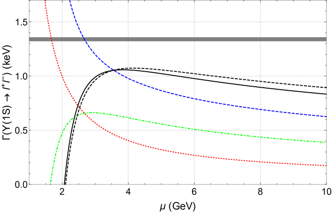
Figure 4: The decay rate obtained from scenario A in the OS scheme as a function of the renormalization scale $\mu$. Dotted (red), dash-dotted (green), short-dashed (blue) and solid (black) lines correspond to LO, NLO, NNLO and N³LO predictions. At N³LO we also show the result from scenario B as black dashed curve. The horizontal bar denotes the experimental value for $\Gamma(\Upsilon(1S)\to e^{+}e^{-})$.

In Fig. 4 we show the dependence of $\Gamma(\Upsilon(1S)\to e^{+}e^{-})|_{\mathrm{pole,A}}$ on $\mu$ successively including higher order corrections. The solid black line corresponds to the N³LO prediction. We observe that the inclusion of higher order corrections clearly stabilizes the perturbative predictions for $\mu\;\hbox to0.0pt{\lower 3.5pt\hbox{$\mathchar 0\relax\sim$}\hss}\raise 1.0pt\hbox{$>$}\;3$ GeV. Furthermore, it is interesting to note that the third-order corrections vanishes close to the value of $\mu$ where the N³LO curve has a maximum. The dashed black curve corresponds to the N³LO prediction of scenario B. The overall shape is very similar to the corresponding curve of scenario A. However, it is remarkable that the two N³LO lines cross the NNLO curve for the same value of $\mu$.

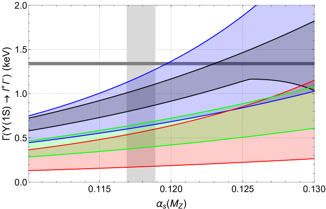
Figure 5: The decay rate obtained from scenario A in the OS scheme as a function of $\alpha_{s}(M_{Z})$ at LO (red, bottom), NLO (green, middle), NNLO (blue, top), and N³LO (black, inner top band). The bands denote the variation of $\mu$ between 3 GeV and 10 GeV. The horizontal bar denotes the experimental value, while the vertical bar denotes the world average of the strong coupling constant, $\alpha_{s}(M_{Z})=0.1179(10)$.

In Fig. 5 we show $\Gamma(\Upsilon(1S)\to e^{+}e^{-})|_{\mathrm{pole,A}}$ as a function of $\alpha_{s}^{(5)}(M_{Z})$. One observes that the third-order band is embedded by the NNLO band which can be interpreted as good convergence of the perturbative corrections. Note that we do not recompute the bottom pole mass when varying $\alpha_{s}$.

It is well-known that the pole mass suffers from so-called renormalon ambiguities. They are avoided by choosing a properly defined so-called threshold mass. Such masses have the advantages that they have nice convergence properties (as the $\overline{\rm MS}$ mass) and that they can also be used for the description of bound-state properties. In the following we want to consider the potential-subtracted (PS) mass scheme Beneke:1998rk as an example and discuss the perturbative corrections to $\Gamma(\Upsilon(1S)\to\ell^{+}\ell^{-})$.

Explicit results for the relation between the pole mass and the PS mass to $n$-th order can be derived from the $n$-loop expression for the Coulomb potential (see for example Ref. Beneke:2005hg ). For scenario A, we use this relation for $n=3$ and $n_{l}=3$, since in this scenario finite charm-quark mass effects are only included in the relation between the $\overline{\rm MS}$ mass and pole mass. In scenario B, however, we also have to include charm-mass effects in the relation between the pole mass and PS mass for $n=1$ and $n=2$. The latter can be found in Appendix B of Ref. Beneke:2014pta .

The numerical (input) value for the PS mass is conveniently obtained from $\bar{m}_{b}(\bar{m}_{b})=4.163$ GeV. Using N³LO accuracy we obtain for the two scenarios $m_{b}^{\mathrm{PS}}|_{A}=4.520$ GeV and $m_{b}^{\mathrm{PS}}|_{B}=4.484$ GeV, respectively, where the factorization scale $\mu_{f}$ is set to 2 GeV. For the decay rate of the $\Upsilon(1S)$ we obtain

$$\Gamma(\Upsilon(1S)\to\ell^{+}\ell^{-})|_{\mathrm{PS,A}} = \frac{2^{5}\alpha^{2}\alpha_{s}^{3}m_{b}}{3^{5}}\left[1+0.485+(1.001+0.017_{c_{v}})+0.125\right]$$

$$= 1.076+0.007_{c_{v}}$$

$$= [1.083\pm 0.053(\alpha_{s}){}^{+0.001}_{-0.270}(\mu)]~{}\mbox{keV}\,,$$

$$\Gamma(\Upsilon(1S)\to\ell^{+}\ell^{-})|_{\mathrm{PS,B}} = \frac{2^{5}\alpha^{2}\alpha_{s}^{3}m_{b}}{3^{5}}\left[1+(0.374+0.042_{m_{c}})+(0.939+0.048_{m_{c}})-0.029\right]$$ (33)

$$= 1.050+0.041_{m_{c}}$$

$$= [1.091\pm 0.052(\alpha_{s}){}^{+0.006}_{-0.218}(\mu)]~{}\mbox{keV}\,.$$

The final predictions for the decay rate are close to those in the on-shell scheme (cf. Eqs. (32)) and agree well within the uncertainties. However, the transition from the pole to the PS mass leads to a significant redistribution among the various perturbative orders. For example, in scenario A the N³LO term in the PS scheme is about four times larger as compared to the on-shell scheme but has a different sign. Similarly, in scenario B the N³LO coefficient gets reduced by a factor six.

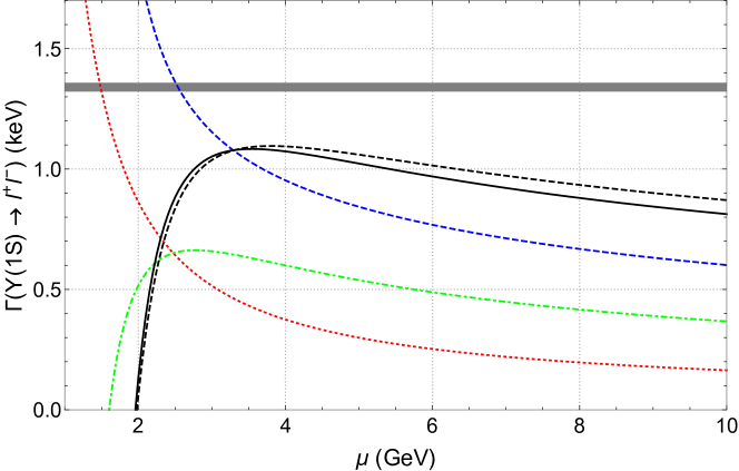
Figure 6: The decay rate obtained from scenario A in the PS scheme as a function of the renormalization scale $\mu$. Dotted (red), dash-dotted (green), short-dashed (blue) and solid (black) lines correspond to LO, NLO, NNLO and N³LO predictions. At N³LO we also show the result from scenario B as black dashed curve. The horizontal bar denotes the experimental value for $\Gamma(\Upsilon(1S)\to e^{+}e^{-})$.

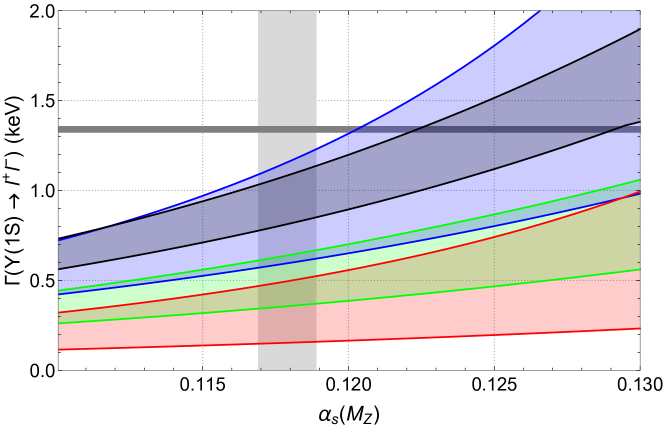
Figure 7: The decay rate obtained from scenario A in the PS scheme as a function of $\alpha_{s}(M_{Z})$ at LO (red, bottom), NLO (green, middle), NNLO (blue, top), and N³LO (black, inner top band). The bands denote the variation of $\mu$ between 3 GeV and 10 GeV. The horizontal bar denotes the experimental value, while the vertical bar denotes the world average of the strong coupling constant, $\alpha_{s}(M_{Z})=0.1179(10)$.

For completeness we show in Figs. 6 and 7 the dependence of $\Gamma(\Upsilon(1S)\to\ell^{+}\ell^{-})$ in the PS scheme on $\mu$ and $\alpha_{s}^{(5)}(M_{Z})$, respectively. The behaviour of the various perturbative orders and the interpretation of the results is very similar to Figs. 4 and 5.

The inclusion of the finite-$m_{c}$ effects leads to the same conclusions as in Ref. Beneke:2014qea : The perturbative predictions for $\Gamma(\Upsilon(1S)\to\ell^{+}\ell^{-})$ are well under control but there is a discrepancy with respect to the experimental result. In Beneke:2014qea one can find an extensive discussion on possible non-perturbative effects. However, no clear conclusion can be drawn and it remains an open question whether a full quantitative understanding of the decay rate based on perturbative and non-perturbative QCD is possible.

V $\Gamma(J/\Psi\to\ell^{+}\ell^{-})$ at N³LO

In this section we apply the formalism of Ref. Beneke:2014qea to the decay of the $J/\Psi$ to massless leptons. In general, the application to charm bound states is questionable, since the ultra-soft scale in PNRQCD is smaller then $\Lambda_{\rm QCD}$. Furthermore, even the hard scale ($m_{c}$) is below 2 GeV. Nevertheless, it is interesting to study the perturbative behaviour and to compare with the experimental result.

Figure 8: The decay rate $\Gamma(J/\Psi\to\ell^{+}\ell^{-})$ in the OS scheme as a function of the renormalization scale $\mu$. Dotted (red), dash-dotted (green), short-dashed (blue) and solid (black) lines correspond to LO, NLO, NNLO and N³LO prediction. The horizontal bar denotes the experimental value for $\Gamma(J/\Psi\to e^{+}e^{-})$.

We work with an on-shell charm quark mass value $m_{c}=1.65$ GeV and choose $\mu=2$ GeV for the renormalization scale. This leads to $\alpha_{s}^{(3)}(2\,\mbox{GeV})=0.2943$. For the decay rate we have

$$\Gamma(J/\Psi\to\ell^{+}\ell^{-})|_{\mathrm{pole}} = \frac{4\,2^{5}\alpha^{2}\alpha_{s}^{3}m_{c}}{3^{5}}\left[1+0.875+1.596+0.654\right]$$ (34)

$$= [5.08\pm 0.35(\alpha_{s}){}^{+0.03}_{-2.25}(\mu)]~{}\mbox{keV}\,,$$

where the scale uncertainty is computed from the variation of $\mu$ in the range $\mu\in[1.5,6]\,\mbox{GeV}$. Although the perturbative series does not converge it is instructive to compare to the experimental result. This is done in Fig. 8 where $\Gamma(J/\Psi\to\ell^{+}\ell^{-})$ is shown as a function of $\mu$. It is interesting to notice that there is agreement between the N³LO prediction and the experimental result $\Gamma(J/\Psi\to\ell^{+}\ell^{-})|_{\mathrm{exp}}=5.53\pm 0.10$ keV Zyla:2020zbs close to the value of $\mu$ where the N³LO curve has a maximum and thus the derivative with respect to $\mu$ vanishes. Furthermore, for this value of $\mu$ the third-order corrections are are quite small, as can be seen from Eq. (34). Note that the N³LO corrections vanish for $\mu=1.724$ GeV. For this value of the renormalization scale we have $\Gamma(J/\Psi\to\ell^{+}\ell^{-})|_{\mathrm{pole}}=5.03$ keV. From Fig. 8 we also observe that even the N³LO curve shows a sizable dependence on $\mu$. Furthermore, one notices that below $\mu\approx 1.5~{}\mbox{GeV}\approx m_{c}$ perturbation theory breaks down.

We want to remark that a similar feature has been observed in Ref. Kniehl:2003ap where next-to-leading logarithmic (NLL) corrections to the hyperfine splitting of heavy quark-antiquark bound states have been considered. The application to the 1S charmonium states shows good agreement for values of the renormalization scale where the NNL prediction has a maximum. The perturbative uncertainties are sizeable, as for the $J/\Psi$ decay rate.

A recent lattice computation of the leptonic decay width is given by $\Gamma(J/\Psi\to e^{+}e^{-})=5.637\pm 0.049$ Hatton:2020qhk , in agreement with the experimental value Zyla:2020zbs .

VI Conclusions

In this paper we consider the matching coefficients between QCD and NRQCD of external vector, axial-vector, scalar and pseudo-scalar currents. We compute all two-loop contributions which involve two mass scales, one from the external quarks and one present in a closed fermion loop. Whereas for the vector current only non-singlet contributions have to be considered there are also singlet contributions for the other three currents. We present analytic results including terms of order $\epsilon$, which are of relevance for a future three-loop calculation.

In Sections IV and V we apply our results for the vector current to the leptonic decay rates of the lowest spin-1 heavy-quark-anti-quark mesons, $\Upsilon(1S)$ and $J/\Psi$, and provide update numerical predictions. We discuss the decay rate $\Gamma(\Upsilon(1S)\to\ell^{+}\ell^{-})$, including charm quark mass effects, both in the three- and four-flavour scheme and for the heavy quark masses defined both in the on-shell and PS scheme. Although there is a good convergence of the perturbative corrections, we observe a discrepancy with respect to the experimental result which to date is not understood.

Appendix A Analytic results for $c_{a}$, $c_{s}$ and $c_{p}$

In this appendix we present analytic results for the two-mass matching coefficients for axial-vector, scalar and pseudo-scalar external currents. The non-singlet results are given by

$$c_{a,\rm non-sing}^{(2)}\Big{|}_{m_{2}} = n_{m}C_{F}T_{F}\Bigg{[}\frac{37}{72}+\frac{41x^{2}}{24}+\pi^{2}\bigg{(}\frac{1}{32x}-\frac{5x}{48}-\frac{19x^{3}}{32}+\frac{2x^{4}}{9}\bigg{)}+\frac{1}{24}\big{(}13+25x^{2}\big{)}H_{0}+\frac{4}{3}x^{4}H_{0}^{2}$$

$$\mbox{}+\bigg{(}\frac{1}{16x}-\frac{5x}{24}-\frac{19x^{3}}{16}+\frac{4x^{4}}{3}\bigg{)}H_{0}H_{1}+\bigg{(}-\frac{1}{16x}+\frac{5x}{24}+\frac{19x^{3}}{16}-\frac{4x^{4}}{3}\bigg{)}H_{0,1}$$

$$\mbox{}+\bigg{(}\frac{1}{16x}-\frac{5x}{24}-\frac{19x^{3}}{16}-\frac{4x^{4}}{3}\bigg{)}H_{-1,0}+\frac{1}{3}\log\bigg{(}\frac{\mu^{2}}{m_{2}^{2}}\bigg{)}\Bigg{]}\,,$$

$$c_{s,\rm non-sing}^{(2)}\Big{|}_{m_{2}} = n_{m}C_{F}T_{F}\Bigg{[}-\frac{1}{72}+\frac{27x^{2}}{8}+\pi^{2}\bigg{(}\frac{1}{32x}+\frac{x}{16}-\frac{35x^{3}}{32}+\frac{x^{4}}{3}\bigg{)}+\frac{1}{24}\big{(}5+57x^{2}\big{)}H_{0}+2x^{4}H_{0}^{2}$$

$$\mbox{}+\bigg{(}\frac{1}{16x}+\frac{x}{8}-\frac{35x^{3}}{16}+2x^{4}\bigg{)}H_{0}H_{1}+\bigg{(}-\frac{1}{16x}-\frac{x}{8}+\frac{35x^{3}}{16}-2x^{4}\bigg{)}H_{0,1}$$

$$\mbox{}+\bigg{(}\frac{1}{16x}+\frac{x}{8}-\frac{35x^{3}}{16}-2x^{4}\bigg{)}H_{-1,0}+\frac{1}{6}\log\bigg{(}\frac{\mu^{2}}{m_{2}^{2}}\bigg{)}\Bigg{]}\,,$$

$$c_{p,\rm non-sing}^{(2)}\Big{|}_{m_{2}} = n_{m}C_{F}T_{F}\Bigg{[}\frac{11}{24}+\frac{25x^{2}}{8}+\pi^{2}\bigg{(}\frac{3}{32x}-\frac{x}{16}-\frac{33x^{3}}{32}+\frac{x^{4}}{3}\bigg{)}+\frac{1}{8}\big{(}5+17x^{2}\big{)}H_{0}+2x^{4}H_{0}^{2}$$ (35)

$$\mbox{}+\bigg{(}\frac{3}{16x}-\frac{x}{8}-\frac{33x^{3}}{16}+2x^{4}\bigg{)}H_{0}H_{1}+\bigg{(}-\frac{3}{16x}+\frac{x}{8}+\frac{33x^{3}}{16}-2x^{4}\bigg{)}H_{0,1}$$

$$\mbox{}+\bigg{(}\frac{3}{16x}-\frac{x}{8}-\frac{33x^{3}}{16}-2x^{4}\bigg{)}H_{-1,0}+\frac{1}{2}\log\bigg{(}\frac{\mu^{2}}{m_{2}^{2}}\bigg{)}\Bigg{]}\,,$$

where $H_{\vec{a}}=H_{\vec{a}}(x)$.

Our results for the pseudo-scalar singlet contribution reads

$$c_{p,\rm sing}^{(2)}\Big{|}_{m_{2}} = n_{m}C_{F}T_{F}\Bigg{[}\pi^{2}\bigg{(}\frac{7t^{3}}{3\big{(}1+t^{2}\big{)}^{3}}+\frac{2tH_{\{4,1\}}}{1+t^{2}}\bigg{)}-\frac{4t^{3}H_{0}}{\big{(}1+t^{2}\big{)}^{2}}+\frac{4t^{3}H_{0}^{2}}{\big{(}1+t^{2}\big{)}^{3}}+\frac{16t^{3}H_{0}H_{1}}{\big{(}1+t^{2}\big{)}^{3}}$$ (36)

$$\mbox{}+\log(2)\bigg{(}-\frac{2t}{1+t^{2}}+\frac{16t^{3}H_{0}}{\big{(}1+t^{2}\big{)}^{3}}+\frac{16t^{3}H_{1}}{\big{(}1+t^{2}\big{)}^{3}}-\frac{16t^{3}H_{-1}}{\big{(}1+t^{2}\big{)}^{3}}\bigg{)}+\bigg{(}\frac{4t}{1+t^{2}}-\frac{8tH_{0}^{2}}{1+t^{2}}\bigg{)}H_{\{4,1\}}$$

$$\mbox{}-\frac{16t^{3}H_{0,1}}{\big{(}1+t^{2}\big{)}^{3}}+\bigg{(}-\frac{32t^{3}}{\big{(}1+t^{2}\big{)}^{3}}+\frac{24tH_{0}}{1+t^{2}}\bigg{)}H_{0,\{4,1\}}-\frac{32t^{3}H_{1,\{4,1\}}}{\big{(}1+t^{2}\big{)}^{3}}-\frac{16t^{3}H_{-1,0}}{\big{(}1+t^{2}\big{)}^{3}}$$

$$\mbox{}+\frac{32t^{3}H_{-1,\{4,1\}}}{\big{(}1+t^{2}\big{)}^{3}}-\frac{24tH_{0,0,\{4,1\}}}{1+t^{2}}+\frac{8t^{3}\log^{2}(2)}{\big{(}1+t^{2}\big{)}^{3}}-\frac{3t\zeta(3)}{1+t^{2}}$$

$$\mbox{}+i\pi\Biggl{\{}-\frac{(-1+t)t(1+t)}{\big{(}1+t^{2}\big{)}^{2}}-\frac{4t^{3}H_{0}}{\big{(}1+t^{2}\big{)}^{3}}-\frac{8tH_{0}H_{\{4,1\}}}{1+t^{2}}+\frac{12tH_{0,\{4,1\}}}{1+t^{2}}\Biggr{\}}\Bigg{]}\,.$$

For the expansions around $x=0$ and $x=1$ we find

$$c_{p,{\rm sing}}^{(2)}\Big{|}_{m_{2},x\to 0} = n_{m}C_{F}T_{F}\Bigg{[}x\bigg{(}-\log(2)-\frac{3\zeta(3)}{2}\bigg{)}+x^{3}\bigg{(}-\frac{1}{8}+\frac{5\pi^{2}}{12}-\frac{\log(2)}{4}-\log^{2}(2)+\frac{1}{4}(1+8\log(2))\log(x)\bigg{)}$$ (37)

$$\mbox{}+i\pi\biggl{\{}\frac{1}{2}x+x^{3}\bigg{(}\frac{1}{8}+\log(2)-\log(x)\bigg{)}\biggr{\}}+\mathcal{O}(x^{4})\Bigg{]}\,,$$

$$c_{p,{\rm sing}}^{(2)}\Big{|}_{m_{2},x\to 1} = n_{m}C_{F}T_{F}\Bigg{[}\frac{5\pi^{2}}{24}+\frac{1}{2}\pi^{2}\log(2)-\frac{21\zeta(3)}{8}-\sqrt{y}\frac{\pi^{2}}{\sqrt{2}}+y\bigg{(}-1-\frac{\pi^{2}}{8}+2\log(2)-\frac{1}{2}\pi^{2}\log(2)+\frac{21\zeta(3)}{8}\bigg{)}$$ (38)

$$\mbox{}+y^{3/2}\frac{7\pi^{2}}{12\sqrt{2}}+y^{2}\bigg{(}\frac{1}{3}+\frac{3\pi^{2}}{8}-\frac{\log(2)}{3}\bigg{)}+y^{5/2}\frac{71\pi^{2}}{480\sqrt{2}}$$

$$\mbox{}+i\pi\biggl{\{}\frac{\pi^{2}}{8}+\sqrt{y}\bigg{(}\sqrt{2}-\sqrt{2}\log(2)\bigg{)}+y\bigg{(}-1-\frac{\pi^{2}}{8}\bigg{)}+y^{3/2}\bigg{(}-\frac{11}{6\sqrt{2}}+\frac{7}{6\sqrt{2}}\log(2)\bigg{)}+\frac{y^{2}}{6}$$

$$\mbox{}+y^{5/2}\bigg{(}\frac{433}{240\sqrt{2}}+\frac{71}{240\sqrt{2}}\log(2)\bigg{)}\biggr{\}}+\mathcal{O}(y^{3})\Bigg{]}\,,$$

with $y=1-x$.

In the case of the singlet axial-vector current we explicitly specify the flavour of the quark in the final state to bottom quark. Furthermore, we split the matching coefficient into the contributions from the strange and charm quarks $c_{a,\rm sing}^{(2),s+c}\Big{|}_{m_{2}}$ and the contribution from the bottom and top quarks $c_{a,\rm sing}^{(2),b+t}\Big{|}_{m_{2}}$. For vanishing strange quark mass we have

$$c_{a,\rm sing}^{(2),s+c}\Big{|}_{m_{2}} = n_{m}C_{F}T_{F}\Bigg{[}\pi^{2}\bigg{(}-\frac{t^{2}\big{(}1+25t^{2}+19t^{4}+9t^{6}\big{)}}{9\big{(}1+t^{2}\big{)}^{4}}+\frac{2t^{2}H_{1}}{3\big{(}1+t^{2}\big{)}^{2}}+\frac{8t^{2}H_{\{4,1\}}}{3\big{(}1+t^{2}\big{)}^{2}}+\frac{2t^{2}H_{-1}}{\big{(}1+t^{2}\big{)}^{2}}\bigg{)}$$ (39)

$$\mbox{}+\log(2)\bigg{(}\frac{4t^{2}}{3\big{(}1+t^{2}\big{)}^{2}}-\frac{8t^{4}\big{(}5+2t^{2}+t^{4}\big{)}H_{0}}{3\big{(}1+t^{2}\big{)}^{4}}+\bigg{(}-\frac{4\big{(}1+2t^{2}+10t^{4}+2t^{6}+t^{8}\big{)}}{3\big{(}1+t^{2}\big{)}^{4}}+\frac{16t^{2}H_{-1}}{3\big{(}1+t^{2}\big{)}^{2}}\bigg{)}H_{1}$$

$$\mbox{}+\frac{8t^{2}H_{1}^{2}}{3\big{(}1+t^{2}\big{)}^{2}}+\frac{4\big{(}1+2t^{2}+10t^{4}+2t^{6}+t^{8}\big{)}H_{-1}}{3\big{(}1+t^{2}\big{)}^{4}}+\frac{8t^{2}H_{-1}^{2}}{3\big{(}1+t^{2}\big{)}^{2}}\bigg{)}+\frac{4t^{2}\big{(}3+8t^{2}+3t^{4}\big{)}H_{0}}{3\big{(}1+t^{2}\big{)}^{3}}$$

$$\mbox{}+\frac{4t^{4}\big{(}-1+2t^{2}+t^{4}\big{)}H_{0}^{2}}{3\big{(}1+t^{2}\big{)}^{4}}+\bigg{(}\frac{4\big{(}-3-6t^{2}-10t^{4}+2t^{6}+t^{8}\big{)}H_{0}}{3\big{(}1+t^{2}\big{)}^{4}}+\frac{8t^{2}H_{0}^{2}}{3\big{(}1+t^{2}\big{)}^{2}}\bigg{)}H_{1}$$

$$\mbox{}+\frac{8t^{2}H_{0}H_{1}^{2}}{3\big{(}1+t^{2}\big{)}^{2}}+\bigg{(}-\frac{4\big{(}-3-6t^{2}-10t^{4}+2t^{6}+t^{8}\big{)}}{3\big{(}1+t^{2}\big{)}^{4}}-\frac{16t^{2}H_{0}}{\big{(}1+t^{2}\big{)}^{2}}-\frac{16t^{2}H_{1}}{3\big{(}1+t^{2}\big{)}^{2}}\bigg{)}H_{0,1}$$

$$\mbox{}+\bigg{(}-\frac{4\big{(}3+8t^{2}+3t^{4}\big{)}}{3\big{(}1+t^{2}\big{)}^{2}}-\frac{32t^{2}H_{0}^{2}}{3\big{(}1+t^{2}\big{)}^{2}}\bigg{)}H_{\{4,1\}}+\bigg{(}\frac{16t^{4}\big{(}5+2t^{2}+t^{4}\big{)}}{3\big{(}1+t^{2}\big{)}^{4}}+\frac{32t^{2}H_{0}}{\big{(}1+t^{2}\big{)}^{2}}\bigg{)}H_{0,\{4,1\}}$$

$$\mbox{}+\frac{8\big{(}1+2t^{2}+10t^{4}+2t^{6}+t^{8}\big{)}H_{1,\{4,1\}}}{3\big{(}1+t^{2}\big{)}^{4}}+\bigg{(}-\frac{8\big{(}1+2t^{2}+10t^{4}+2t^{6}+t^{8}\big{)}}{3\big{(}1+t^{2}\big{)}^{4}}-\frac{32t^{2}H_{1}(t)}{3\big{(}1+t^{2}\big{)}^{2}}\bigg{)}H_{-1,\{4,1\}}$$

$$\mbox{}+\bigg{(}-\frac{4\big{(}-3-6t^{2}-10t^{4}+2t^{6}+t^{8}\big{)}}{3\big{(}1+t^{2}\big{)}^{4}}+\frac{32t^{2}H_{0}}{3\big{(}1+t^{2}\big{)}^{2}}+\frac{16t^{2}H_{1}}{3\big{(}1+t^{2}\big{)}^{2}}\bigg{)}H_{-1,0}+\frac{80t^{2}H_{0,0,1}}{3\big{(}1+t^{2}\big{)}^{2}}$$

$$\mbox{}-\frac{128t^{2}H_{0,0,\{4,1\}}}{3\big{(}1+t^{2}\big{)}^{2}}+\frac{16t^{2}H_{0,1,1}(t)}{3\big{(}1+t^{2}\big{)}^{2}}-\frac{32t^{2}H_{1,1,\{4,1\}}}{3\big{(}1+t^{2}\big{)}^{2}}-\frac{80t^{2}H_{-1,0,0}}{3\big{(}1+t^{2}\big{)}^{2}}-\frac{16t^{2}H_{-1,0,1}}{3\big{(}1+t^{2}\big{)}^{2}}+\frac{32t^{2}H_{-1,\{4,1\},1}}{3\big{(}1+t^{2}\big{)}^{2}}$$

$$\mbox{}+\frac{16t^{2}H_{-1,-1,0}}{3\big{(}1+t^{2}\big{)}^{2}}-\frac{32t^{2}H_{-1,-1,\{4,1\}}}{3\big{(}1+t^{2}\big{)}^{2}}+\frac{4(-1+t)^{2}t^{2}(1+t)^{2}\log^{2}(2)}{3\big{(}1+t^{2}\big{)}^{4}}-\frac{5t^{2}\zeta(3)}{\big{(}1+t^{2}\big{)}^{2}}$$

$$\mbox{}+i\pi\Biggl{\{}\frac{\pi^{2}t^{2}}{3\big{(}1+t^{2}\big{)}^{2}}+\frac{2t^{2}\big{(}2+t^{2}\big{)}\big{(}1+3t^{2}\big{)}}{3\big{(}1+t^{2}\big{)}^{3}}+\bigg{(}\frac{8t^{4}\big{(}2+2t^{2}+t^{4}\big{)}}{3\big{(}1+t^{2}\big{)}^{4}}+\frac{16t^{2}H_{-1}}{3\big{(}1+t^{2}\big{)}^{2}}\bigg{)}H_{0}$$

$$\mbox{}+\bigg{(}\frac{4(-1+t)(1+t)}{3\big{(}1+t^{2}\big{)}}+\frac{8t^{2}H_{0}}{3\big{(}1+t^{2}\big{)}^{2}}\bigg{)}H_{1}-\frac{32t^{2}H_{0}H_{\{4,1\}}}{3\big{(}1+t^{2}\big{)}^{2}}-\frac{4(-1+t)(1+t)H_{-1}}{3\big{(}1+t^{2}\big{)}}$$

$$\mbox{}-\frac{8t^{2}H_{0,1}}{\big{(}1+t^{2}\big{)}^{2}}+\frac{16t^{2}H_{0,\{4,1\}}}{\big{(}1+t^{2}\big{)}^{2}}-\frac{8t^{2}H_{-1,0}}{\big{(}1+t^{2}\big{)}^{2}}-\frac{4t^{2}\log(2)}{3\big{(}1+t^{2}\big{)}}\Biggr{\}}\Bigg{]}\,,$$

with $t=(1-\sqrt{1-x_{c}^{2}})/x_{c}$ and $x_{c}=m_{c}/m_{b}$. The expansion of $x_{c}\to 0$ is given by

$$c_{a,\rm sing}^{(2),s+c}\Big{|}_{m_{2},x_{c}\to 0} = n_{m}C_{F}T_{F}\Bigg{[}x_{c}^{2}\biggl{(}-\frac{\pi^{2}}{36}+\frac{1}{3}\log^{2}(2)-\frac{5}{4}\zeta(3)+i\pi\biggl{[}\frac{\pi^{2}}{12}-\frac{1}{3}\log(2)\biggr{]}\biggr{)}+\frac{\pi^{2}}{3}x_{c}^{3}+\mathcal{O}(x_{c}^{4})\Bigg{]}$$ (40)

Due to the large mass of the top quark it is convenient to provide for $c_{a,\rm sing}^{(2),{b+t}}|_{m_{2}}$ only the first few expansion terms in $x_{t}=m_{b}/m_{t}$. Our results read

$$c_{a,\rm sing}^{(2),{b+t}}\Big{|}_{m_{2}} = n_{m}C_{F}T_{F}\Bigg{[}\frac{55}{24}-\frac{3}{2}\log(x_{t})+\pi^{2}\biggl{(}\frac{19}{72}-\frac{2}{3}\log(2)\biggr{)}-x_{t}^{2}\biggl{(}\frac{47}{216}+\frac{5}{18}\log(x_{t})\biggr{)}$$ (41)

$$\mbox{}-x_{t}^{4}\biggl{(}\frac{1337}{21600}+\frac{23}{108}\log(x_{t})\biggr{)}+\mathcal{O}(x_{t}^{6})\Biggr{]}\,.$$

In progdata computer-readable expressions for the four non-singlet and the three singlet matching coefficients are provided. We include terms or order $\epsilon$, which are needed for a future three-loop calculation.

References

References

- (1) M. Beneke, Y. Kiyo, P. Marquard, A. Penin, J. Piclum, D. Seidel and M. Steinhauser, Phys. Rev. Lett. 112 (2014) no.15, 151801 [arXiv:1401.3005 [hep-ph]].
- (2) A. Pineda, Prog. Part. Nucl. Phys. 67 (2012), 735-785 [arXiv:1111.0165 [hep-ph]].
- (3) M. Beneke, Y. Kiyo and K. Schuller, [arXiv:1312.4791 [hep-ph]].
- (4) M. Beneke, Y. Kiyo and K. Schuller, Phys. Lett. B 658, 222 (2008), arXiv:0705.4518 [hep-ph].
- (5) A. Czarnecki and K. Melnikov, Phys. Rev. Lett. 80 (1998), 2531-2534 [arXiv:hep-ph/9712222 [hep-ph]].
- (6) M. Beneke, A. Signer and V. A. Smirnov, Phys. Rev. Lett. 80 (1998), 2535-2538 [arXiv:hep-ph/9712302 [hep-ph]].
- (7) P. Marquard, J. H. Piclum, D. Seidel and M. Steinhauser, Phys. Rev. D 89 (2014) no.3, 034027 [arXiv:1401.3004 [hep-ph]].
- (8) M. Beneke, Y. Kiyo and A. A. Penin, Phys. Lett. B 653, 53 (2007), arXiv:0706.2733 [hep-ph].
- (9) M. Beneke, A. Maier, J. Piclum and T. Rauh, Nucl. Phys. B 891 (2015), 42-72 [arXiv:1411.3132 [hep-ph]].
-
(10)
https://www.ttp.kit.edu/preprints/2021/ttp21-012/. - (11) M. Beneke and V. A. Smirnov, Nucl. Phys. B 522, 321 (1998) [hep-ph/9711391].
- (12) V. A. Smirnov, Springer Tracts Mod. Phys. 177 (2002), 1-262
- (13) A. V. Smirnov and F. S. Chuharev, Comput. Phys. Commun. 247 (2020), 106877 [arXiv:1901.07808 [hep-ph]].
- (14) R. N. Lee, arXiv:1212.2685 [hep-ph].
- (15) C. Meyer, Comput. Phys. Commun. 222 (2018), 295-312 [arXiv:1705.06252 [hep-ph]].
- (16) E. Remiddi and J. A. M. Vermaseren, Int. J. Mod. Phys. A 15 (2000), 725-754 [arXiv:hep-ph/9905237 [hep-ph]].
- (17) A. G. Grozin, P. Marquard, A. V. Smirnov, V. A. Smirnov and M. Steinhauser, Phys. Rev. D 102 (2020) no.5, 054008 [arXiv:2005.14047 [hep-ph]].
- (18) D. J. Broadhurst, N. Gray and K. Schilcher, Z. Phys. C 52 (1991), 111-122
- (19) S. Bekavac, A. Grozin, D. Seidel and M. Steinhauser, JHEP 10 (2007), 006 [arXiv:0708.1729 [hep-ph]].
- (20) A. I. Davydychev and A. G. Grozin, Phys. Rev. D 59 (1999), 054023 [arXiv:hep-ph/9809589 [hep-ph]].
- (21) M. Fael, K. Schönwald and M. Steinhauser, JHEP 10 (2020), 087 [arXiv:2008.01102 [hep-ph]].
- (22) B. A. Kniehl, A. Onishchenko, J. H. Piclum and M. Steinhauser, Phys. Lett. B 638 (2006), 209-213 [arXiv:hep-ph/0604072 [hep-ph]].
- (23) S. A. Larin, Phys. Lett. B 303 (1993), 113-118 [arXiv:hep-ph/9302240 [hep-ph]].
- (24) J. Vermaseren, Int. J. Mod. Phys. A 14 (1999), 2037-2076 [arXiv:hep-ph/9806280 [hep-ph]]; E. Remiddi and J. Vermaseren, Int. J. Mod. Phys. A 15 (2000), 725-754 [arXiv:hep-ph/9905237 [hep-ph]]; J. Blümlein, Comput. Phys. Commun. 180 (2009), 2218-2249 [arXiv:0901.3106 [hep-ph]]; J. Ablinger, Diploma Thesis, J. Kepler University Linz, 2009, arXiv:1011.1176 [math-ph]; J. Ablinger, J. Blümlein and C. Schneider, J. Math. Phys. 52 (2011) 102301 [arXiv:1105.6063 [math-ph]]; J. Ablinger, J. Blümlein and C. Schneider, J. Math. Phys. 54 (2013), 082301 [arXiv:1302.0378 [math-ph]]; J. Ablinger, Ph.D. Thesis, J. Kepler University Linz, 2012, arXiv:1305.0687 [math-ph]; J. Ablinger, J. Blümlein and C. Schneider, J. Phys. Conf. Ser. 523 (2014), 012060 [arXiv:1310.5645 [math-ph]]; J. Ablinger, J. Blümlein, C. Raab and C. Schneider, J. Math. Phys. 55 (2014), 112301 [arXiv:1407.1822 [hep-th]]; J. Ablinger, PoS LL2014 (2014), 019 [arXiv:1407.6180 [cs.SC]]; J. Ablinger, [arXiv:1606.02845 [cs.SC]]; J. Ablinger, PoS RADCOR2017 (2017), 069 [arXiv:1801.01039 [cs.SC]]; J. Ablinger, PoS LL2018 (2018), 063; J. Ablinger, [arXiv:1902.11001 [math.CO]].
- (25) J. H. Piclum, “Heavy quark threshold dynamics in higher order,” Dissertation, Hamburg University 2007.
- (26) J. Ablinger, J. Blümlein, P. Marquard, N. Rana and C. Schneider, Nucl. Phys. B 939 (2019), 253-291 [arXiv:1810.12261 [hep-ph]].
- (27) C. Schneider, Sém. Lothar. Combin. 56 (2007) 1, article B56b; C. Schneider, in: Computer Algebra in Quantum Field Theory: Integration, Summation and Special Functions Texts and Monographs in Symbolic Computation eds. C. Schneider and J. Blümlein (Springer, Wien, 2013) 325 arXiv:1304.4134 [cs.SC].
- (28) S. Gerhold, Uncoupling Systems of Linear Ore Operator Equations, Diploma Thesis, RISC, J. Kepler University, Linz, February 2002.
- (29) D. Eiras and J. Soto, Phys. Lett. B 491 (2000), 101-110 [arXiv:hep-ph/0005066 [hep-ph]].
- (30) A. H. Hoang, [arXiv:hep-ph/0008102 [hep-ph]].
- (31) M. Beneke, Y. Kiyo, A. Maier and J. Piclum, Comput. Phys. Commun. 209 (2016), 96-115 [arXiv:1605.03010 [hep-ph]].
- (32) C. Ayala, G. Cvetič and A. Pineda, JHEP 09 (2014), 045 [arXiv:1407.2128 [hep-ph]].
- (33) F. Jegerlehner, Nuovo Cim. C 034S1 (2011), 31-40 [arXiv:1107.4683 [hep-ph]].
- (34) P. A. Zyla et al. [Particle Data Group], PTEP 2020 (2020) no.8, 083C01
- (35) F. Herren and M. Steinhauser, Comput. Phys. Commun. 224 (2018), 333-345 doi:10.1016/j.cpc.2017.11.014 [arXiv:1703.03751 [hep-ph]].
- (36) K. G. Chetyrkin, J. H. Kuhn, A. Maier, P. Maierhofer, P. Marquard, M. Steinhauser and C. Sturm, Phys. Rev. D 80, 074010 (2009) [arXiv:0907.2110 [hep-ph]].
- (37) D. Hatton, C. T. H. Davies, J. Koponen, G. P. Lepage and A. T. Lytle, [arXiv:2101.08103 [hep-lat]].
- (38) M. Beneke, Phys. Lett. B 434, 115 (1998) [hep-ph/9804241].
- (39) M. Beneke, Y. Kiyo and K. Schuller, Nucl. Phys. B 714, 67 (2005) [hep-ph/0501289].
- (40) B. A. Kniehl, A. A. Penin, A. Pineda, V. A. Smirnov and M. Steinhauser, Phys. Rev. Lett. 92 (2004), 242001 [erratum: Phys. Rev. Lett. 104 (2010), 199901] [arXiv:hep-ph/0312086 [hep-ph]].
- (41) D. Hatton et al. [HPQCD], Phys. Rev. D 102 (2020) no.5, 054511 [arXiv:2005.01845 [hep-lat]].