FTPI-MINN-21-07, UMN-TH-4014/21, INR-TH-2021-011 Black hole induced false vacuum decay
from first principles

We provide a method to calculate the rate of false vacuum decay induced by a black hole. The method uses complex tunneling solutions and consistently takes into account the structure of different quantum vacua in the black hole metric via boundary conditions. The latter are connected to the asymptotic behavior of the time-ordered Green’s function in the corresponding vacua. We illustrate the technique on a two-dimensional toy model of a scalar field with inverted Liouville potential in an external background of a dilaton black hole. We analytically derive the exponential suppression of tunneling from the Boulware, Hartle–Hawking and Unruh vacua and show that they are parametrically different. The Unruh vacuum decay rate is exponentially smaller than the decay rate of the Hartle–Hawking state, though both rates become unsuppressed at high enough black hole temperature. We interpret the vanishing suppression of the Unruh vacuum decay at high temperature as an artifact of the two-dimensional model and discuss why this result can be modified in the realistic case of black holes in four dimensions.

1 Introduction and summary

Description of false vacuum decay in the presence of a black hole (BH) is a long-standing problem [1, 2, 3, 4]. The interest in it has been revived in recent years due to its possible phenomenological relevance. The electroweak vacuum determined by the Standard Model Higgs potential may not be absolutely stable [5, 6, 7, 8, 9, 10, 11]. In the absence of excitations its decay rate is exponentially suppressed and its lifetime exceeds the age of the Universe by many orders of magnitude [12]. However, it has been argued in [13, 14, 15, 16] that the decay can be strongly catalyzed if the Universe hosts at some stages of its evolution light primordial BHs that later evaporate via Hawking radiation. Such BHs appear in a variety of early Universe models and can play important roles in cosmology, including reheating of the Universe, production of baryon asymmetry and dark matter, etc. [17, 18, 19, 20, 21, 22, 23, 24] (see also [25] for a review of primordial BH production mechanisms and constraints). The results of Refs. [13, 14, 15, 16] would rule out the presence of any evaporating BHs in our causal past and thereby put stringent constraints on primordial BH models. Or, alternatively, would imply that the Standard Model is completed in the way to prevent the electroweak vacuum instability.

The intuitive reason behind the BH catalysis of vacuum decay is rather simple. Due to the Hawking effect, a BH can be thought of as a body with finite temperature. As the BH evaporates, it heats up scanning all temperatures up to Planckian. On the other hand, it is known that the false vacuum decay becomes unsuppressed at high enough temperatures, comparable to the height of the energy barrier between the false and the true vacuum. The latter height is given by the energy of the sphaleron configuration (also called critical bubble) — static unstable solution of the equations of motion separating the two vacua. Thus, one might expect a BH also to render the decay unsuppressed once it becomes sufficiently hot.

However, the above reasoning has a caveat. A realistic BH is not in thermal equilibrium with its environment. It radiates away a thermal spectrum of particles, but does not receive anything back. From the technical viewpoint, this corresponds to the Unruh vacuum state [27], as opposed to the Hartle–Hawking vacuum [28] describing a BH immersed in a thermal bath with the same temperature. The deviation from equilibrium is expected to reduce the catalyzing effect of BH and it is not clear if it can overcome the exponential suppression of vacuum decay at any BH temperature. The results in the literature addressing this issue have been controversial [29, 30, 31, 32, 33]. Even if the exponential suppression persists for all BHs, it is still important to know how much it is reduced compared to the no-BH case. Indeed, for a given density of primordial BHs, each of them can be a nucleation cite for the vacuum decay bubble. The small probability of this event for a single BH will be multiplied by the huge number of these BHs in the observable Universe [29, 30, 34]. Thus the condition that no vacuum decay occurs in our causal past can still put relevant constraints on the primordial BH scenarios and/or completion of the Standard Model.

Apart from the relevance for phenomenology, BH catalysis of vacuum decay is of considerable theoretical interest. First, its study is expected to give insight into nonperturbative quantum field theory in curved spacetimes with nontrivial causal structure. Second, when the dynamical metric is included, it can teach us about the properties of semiclassical quantum gravity, similarly to Coleman–De Luccia [36] and Hawking–Moss [37] instantons in de Sitter space. Third, Ref. [13] pointed out an intriguing connection between the probability of false vacuum decay and BH entropy, which may shed a new light on the origin of the latter.

All this calls for a self-consistent framework to calculate the effect of BH on vacuum instability that takes into account the properties of the Unruh vacuum. Developing such framework is the purpose of this work. To clarify the analysis, we will consider the dynamical sector consisting of a single scalar field $\varphi$ evolving in a fixed background geometry. Further, for most of the paper we will focus on a setup in two dimensions, commenting on its relation to spherically-symmetric four-dimensional dynamics at the end.

Even with these simplifications, our task is challenging. Being classically forbidden, the false vacuum decay represents a tunneling process. In the semiclassical limit one expects it to be described by a complex solution of the field equations representing the saddle point of the Feynman path integral [38]. The first question that arises is:

• On which section of complexified spacetime coordinates the tunneling solution is defined?

In equilibrium situations the answer to this question is well-known: the tunneling solution lives in purely imaginary (Euclidean) time. The standard way to arrive to these solutions is to work from the beginning with the Euclidean partition function [39, 40, 41]. In the case of a Schwarzschild BH this leads to the theory in the cigar-like geometry with compactified Euclidean time coordinate playing the role of the angular variable and the radial coordinate covering the region outside the horizon [28]. This picture corresponds to the partition function in the Hartle–Hawking vacuum, i.e., an equilibrium thermal state. It is not clear at all how it can be modified to accommodate the Unruh state.

Instead, we use an alternative approach that starts from the path integral expression for the transition amplitude in real time from the false vacuum at $t\to-\infty$ to the true vacuum at $t\to+\infty$. To obtain the tunneling solution, the real time axis is deformed into a contour in the complex time plane, on which the path integral can be evaluated in the saddle-point approximation [42, 43, 44, 45, 46] (see [47, 48, 49, 50] for related approaches). The contour consists of segments parallel to the real axis that are connected by imaginary-time evolution and goes around the singularities of the tunneling solution. This method is very flexible and allows one to fix the initial and final quantum states by an appropriate choice of the boundary conditions at $t\to\mp\infty$. It has been employed to describe baryon number violating processes in the Standard Model [51], false vacuum decay in de Sitter space [52], tunneling induced by particle collisions [53, 54, 55], creation of solitons by highly energetic particles [56, 57, 58], semiclassical black hole S-matrix [59, 60], as well as a variety of transitions in quantum mechanics [61, 62, 63, 64]. In this work we generalize this method to the case of mixed initial states described by a density matrix and show that it naturally fits into the in-in formalism of nonequilibrium quantum field theory. We will see that for equilibrium initial states this method recovers the standard Euclidean results.

It is still not clear at this point what time coordinate one shall use. The nontrivial causal structure of BH spacetime provides several inequivalent choices. First, one can work in Schwarzschild coordinates, in which the metric is static. The latter property appears desirable as it facilitates the analytic continuation into complex time. This coordinate chart, however, is geodesically incomplete covering only the region outside the BH horizon. A second option is presented by Painlevé or Finkelstein coordinates which preserve the stationarity of the metric while extending across the future horizon. The third option is Kruskal coordinates covering the whole maximally extended spacetime at the expense of rendering the metric time-dependent.

The Unruh vacuum is regular at the future BH horizon and is singular at the past horizon. At first sight, this suggests to use the second option above. However, one then encounters the following problem. If one works in the coordinate chart covering the BH interior, it appears that the analysis will depend on what happens inside the BH. Such dependence would be unphysical: the vacuum decay rate measured by an observer outside the BH must be insensitive to the dynamics shielded by the event horizon. Thus, we arrive to our second question:

• Is it possible to formulate the false vacuum decay problem referring only to the region outside the BH horizon?

We answer this question in the affirmative. In fact, we will carry out the whole analysis in the Schwarzschild coordinates and describe the Hartle–Hawking and Unruh vacua as mixed states outside the BH.

In doing so, we will address the third and last question:

• What are the boundary conditions on the tunneling solutions corresponding to different initial vacua?

We derive these boundary conditions by performing a saddle-point integration with the initial-state density matrix. This leads us to linear relations between positive- and negative-frequency components of the field in the asymptotic past. We show that the same relations are obeyed by the mode decompositions of the time-ordered Green’s functions in the respective vacua. In other words, the boundary conditions at $t\to-\infty$ for the tunneling solutions describing decay of a false vacuum are dictated by the time-ordered Green’s function in this vacuum. We argue that this result is general: it is valid for arbitrary geometry and any state with a Gaussian density matrix in the vicinity of the false vacuum. As for the final boundary conditions, we will see that they do not need to be precisely specified. It is enough to require that on the real axis the tunneling solution ends up in the basin of attraction of the true vacuum at $t\to+\infty$.

We provide a detailed illustration of our method using a solvable toy model of a scalar field with inverted Liouville potential and a mass term in two dimensions. We show that different boundary conditions indeed discriminate between different vacuum states and lead to manifestly different decay probabilities. In particular, we find the lifetime of the Unruh vacuum to be exponentially longer than that of the Hartle–Hawking state.

It is worth emphasizing that our method goes in an essential way beyond the thin-wall approximation often used in the literature. Indeed, the boundary conditions for the Unruh vacuum rely on the properties of the solutions to the wave equation that are not captured by the thin-wall Ansatz.

The paper is organized as follows. In Sec. 2 we develop the general formalism for description of vacuum decay in the presence of a BH. For concreteness, we consider a two-dimensional setup with a scalar field $\varphi$ which we introduce in Sec. 2.1. In Sec. 2.2 we discuss the mode decomposition and various vacua, whereas in Sec. 2.3 we present the corresponding Green’s functions. In Sec. 2.4 we formulate the vacuum decay problem using the in-in path integral and relate the boundary conditions for the tunneling solution to the properties of the time-ordered Green’s function.

In Sec. 3 we specify our toy model. To get insight into its dynamics, we first study it in flat geometry. In Sec. 3.1 we find the sphaleron solution separating the false vacuum from the run-away region $\varphi\to+\infty$, which in this model replaces the true vacuum. In Secs. 3.2 and 3.3 we discuss the tunneling solutions describing the false vacuum decay at zero and finite temperature, respectively. We show how the standard results are reproduced using our approach.

In Sec. 4 we consider tunneling in Rindler metric which describes the near-horizon region of a BH. This serves as a warm-up before turning to the full BH case and allows us to develop the necessary intuition. We revisit the decay of Minkowski vacuum from the viewpoint of the Rindler space where it corresponds to nontrivial boundary conditions, analogous to the Hartle–Hawking state in the BH metric [66].

Sec. 5 contains our key results for the toy model. In Sec. 5.1 we calculate the decay rate of the Hartle–Hawking state as a function of BH temperature using our method and show that it recovers the Euclidean result. As expected, the decay rate increases with temperature and becomes unsuppressed when the temperature gets high enough. In Sec. 5.2 we find the tunneling solutions describing the decay of the Unruh vacuum and evaluate their action. We consider both tunneling far away from the BH and in the near-horizon region. In both cases the decay rate is exponentially smaller that the decay rate of the Hartle–Hawking state. Nevertheless, the suppression diminishes with temperature and eventually disappears for sufficiently hot BHs. For completeness, we also consider the Boulware vacuum [67] in Appendix F and show that its decay probability does not essentially differ from that in flat space.

Sec. 6 is devoted to discussion and outlook. In particular, we point out that the vanishing suppression of the Unruh vacuum decay at high BH temperature found in Sec. 5.2 is likely to be a peculiarity of the two-dimensional theory. We highlight the properties of realistic four-dimensional BHs that can alter this behavior.

Several Appendices complement the analysis in the main text.

2 The method

2.1 Setup

We consider a scalar field $\varphi$ in two spacetime dimensions with the action

$$S=\dfrac{1}{\text{g}^{2}}\int d^{2}x\sqrt{-g}\left(-\dfrac{1}{2}g^{\mu\nu}\partial_{\mu}\varphi\partial_{\nu}\varphi-V(\varphi)\right)\;.$$ (2.1)

Note that we have factored out the small coupling constant g in front of the action, which can always be achieved by a field rescaling. This coupling will control the semiclassical expansion in what follows. The potential $V(\varphi)$ is assumed to have a local minimum at $\varphi=0$ where it vanishes, $V(0)=0$. This minimum corresponds to a false vacuum separated from the region $V<0$ by a potential barrier. Two situations are possible: (a) the potential is bounded from below and a true vacuum exists at a finite value $\varphi_{\rm true}$; or (b) the potential is unbounded and the true vacuum is replaced by the run-away $\varphi\to+\infty$. These options are depicted in Fig. 1.

To model the BH geometry, we consider the static metric,

$$ds^{2}=-\Omega(r)\,dt^{2}+\frac{dr^{2}}{\Omega(r)}\;,$$ (2.2)

where the function $\Omega$ approaches 1 at $r\to+\infty$ and has a simple zero at $r=r_{h}$ corresponding to the horizon. Near the horizon it is expanded as

$$\Omega\approx 2\lambda(r-r_{h})~{}~{}~{}~{}\text{at}~{}~{}r\approx r_{h}\;,$$ (2.3)

where the parameter $\lambda$ sets the horizon surface gravity and is related to the BH temperature, $\lambda=2\pi T_{\rm BH}$ (see, e.g., [68]). It is convenient to introduce the “tortoise” coordinate

$$x=\int\frac{dr}{\Omega}\;,$$ (2.4)

in which the metric becomes conformally-flat,

$$ds^{2}=\Omega(x)(-dt^{2}+dx^{2})\;.$$ (2.5)

The horizon is now located at $x\to-\infty$ and in the near-horizon region the metric function has an exponential fall-off,

$$\Omega\approx{\rm e}^{2\lambda x}~{}~{}~{}~{}\text{at}~{}~{}x\to-\infty\;.$$ (2.6)

Explicitly, we will consider the metric of a two-dimensional dilaton BH,

$$\Omega=\big{(}1+{\rm e}^{-2\lambda x}\big{)}^{-1}\;,$$ (2.7)

though most of our analysis will be insensitive to this precise form of the function $\Omega(x)$. Note that while the coordinate size of the near-horizon region in tortoise coordinates is infinite, its physical size is finite and inversely proportional to $\lambda$,

$$l_{h}\sim\int_{-\infty}^{0}\sqrt{\Omega}\,dx\sim\frac{1}{\lambda}\;.$$ (2.8)

With the choice of the metric (2.5) the scalar action becomes

$$S=\dfrac{1}{\text{g}^{2}}\int dtdx\left(-\dfrac{1}{2}\eta^{\mu\nu}\partial_{\mu}\varphi\partial_{\nu}\varphi-\Omega(x)V(\varphi)\right)\;,$$ (2.9)

where $\eta^{\mu\nu}=\text{diag}(-1,1)$ is the two-dimensional Minkowski metric. We observe that the dependence on geometry has been isolated into a position-dependent factor in front of the potential term.

a                       b

Figure 1: Scalar potential with false vacuum at $\varphi=0$. (a) The true vacuum exists at a finite value of the field. (b) The potential is unbounded from below and the false vacuum decay leads to the run-away $\varphi\to+\infty$.

The coordinates $(t,x)$ cover the BH exterior. This corresponds to the region I in the Penrose diagram of the maximally-extended BH spacetime, see Fig. 2. To obtain this maximal extension, one first introduces the light-like coordinates

$$u=t-x\;,~{}~{}~{}~{}v=t+x\;,$$ (2.10)

and then the Kruskal coordinates

$$\bar{u}=-\lambda^{-1}{\rm e}^{-\lambda u}\;,~{}~{}~{}~{}\bar{v}=\lambda^{-1}{\rm e}^{\lambda v}\;.$$ (2.11)

In the new coordinates the metric takes the form

$$ds^{2}=-\frac{d{\bar{u}}d\bar{v}}{1-\lambda^{2}{\bar{u}}\bar{v}}\;,$$ (2.12)

which is regular as long as ${\bar{u}}\bar{v}<1/\lambda^{2}$. The latter condition defines the range of $({\bar{u}},\bar{v})$ values covering the maximally-extended spacetime. In region I we have $-\infty<{\bar{u}}<0$, $0<\bar{v}<+\infty$. The future BH horizon $H^{+}$ corresponds to ${\bar{u}}=0$ and the past horizon $H^{-}$ to $\bar{v}=0$. An important role in our analysis will be played by the past boundary of the region I where we will impose the conditions defining different vacua in the BH background. It consists of the past horizon $H^{-}$, past time-like infinity $i^{-}$ and past light-like infinity ${\cal I}^{-}$.

Figure 2: Penrose diagram of the maximally-extended BH spacetime. The tortoise coordinates $(t,x)$ cover the exterior region I. The conditions defining different vacua in the BH background will be imposed on the past boundary of this region consisting of the past horizon $H^{-}$, past time-like infinity $i^{-}$ and past light-like infinity ${\cal I}^{-}$ (marked by the thick line).

Let us comment on the approximation of static geometry. The metric of a realistic BH will evolve due to its evaporation. Our approximation is valid as long as the evaporation time is larger than the inverse of the energy scale characterizing the vacuum decay. The latter should not be confused with the vacuum decay rate. Rather, it is set by the size of the bubble of the true vacuum inside the false one at the moment of nucleation. On the other hand, the exponentially suppressed decay rate determines the probability of bubble nucleation in a unit time interval. If the inverse decay rate exceeds the BH evaporation time, it just means that the probability for a single BH to catalyze vacuum decay is small. As with any probability, it acquires statistical significance when one considers an ensemble of identical BHs, whose overall catalyzing effect can become sizable due to their large number.

Our analysis does not capture the highly nonstationary stages of BH formation and complete evaporation which may have additional catalyzing effect on vacuum decay. The associated enhancement of the decay rate is expected to depend strongly on the details of these transient events. By contrast, the catalyzing effect of a quasi-stationary BH studied in this paper is universal and accumulates over the whole BH lifetime.

2.2 Mode decomposition and vacua

In this section we study the dynamics of linear perturbations around the false vacuum. Thus, we replace the potential term by the free-field part,

$$V(\varphi)\mapsto m^{2}\varphi^{2}/2\;,$$

where $m$ is the mass of the field in the false vacuum. This leads to the linearized field equation

$$\Box\varphi-m^{2}\Omega\varphi=0\;,$$ (2.13)

where $\Box=\eta^{\mu\nu}\partial_{\mu}\partial_{\nu}$. The false vacuum is a quantum state. To define it, we quantize the field $\varphi$ using a complete set of positive- and negative-frequency modes

$$\varphi^{+}_{\omega}(t,x)=f_{\omega}(x)e^{-i\omega t}~{},~{}~{}~{}~{}~{}\varphi^{-}_{\omega}(t,x)=f^{*}_{\omega}(x)e^{i\omega t}\;,~{}~{}~{}\omega>0\;,$$ (2.14)

where the mode functions $f_{\omega}(x)$ satisfy the eigenvalue equation

$$-\frac{d^{2}f_{\omega}}{dx^{2}}+m^{2}\Omega f_{\omega}=\omega^{2}f_{\omega}\;.$$ (2.15)

This is a Schrödinger equation with the potential $U_{\rm eff}(x)=m^{2}\Omega(x)$. The latter is shown in Fig. 3 for the case of the dilaton BH.

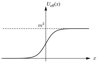
Figure 3: Potential for massive scalar linear modes in the dilaton BH background in two dimensions. The horizon is located at $x\to-\infty$.

At $\omega>m$ equation (2.15) has two linearly-independent solutions which we denote by $f_{R,\omega}$ and $f_{L,\omega}$. The first solution $f_{R,\omega}$ reduces to a right-moving plane wave at large positive $x$: it describes radiation directed outward the BH. In the near-horizon region $x\to-\infty$ it contains both left- and right-moving waves. We have

$$f_{R,\omega}=\begin{cases}\alpha_{\omega}\,{\rm e}^{i\omega x}+\beta_{\omega}\,{\rm e}^{-i\omega x}\;,&x\to-\infty\\ \gamma_{\omega}\,{\rm e}^{ikx}\;,&x\to+\infty\end{cases}$$ (2.16)

where

$$k=\sqrt{\omega^{2}-m^{2}}\;.$$ (2.17)

The second mode $f_{L,\omega}$ becomes a pure left-moving wave at large negative $x$: it describes radiation falling into BH. Far away from the BH it is a sum of two plane waves,

$$f_{L,\omega}=\begin{cases}\tilde{\beta}_{\omega}\,{\rm e}^{-i\omega x}\;,&x\to-\infty\\ \tilde{\gamma}_{\omega}\,{\rm e}^{ikx}+\tilde{\delta}_{\omega}\,{\rm e}^{-ikx}\;,&x\to+\infty\end{cases}\;,\qquad\omega>m\;.$$ (2.18)

The modes $f_{R,\omega}$, $f_{L,\omega}$ are orthogonal to each other,

$$\int_{-\infty}^{\infty}dx\;f_{R,\omega}(x)f^{*}_{L,\omega^{\prime}}(x)=0\;,$$ (2.19)

and are $\delta$-function normalizable. We fix their normalization as follows:

$$\begin{split}&\int_{-\infty}^{\infty}dx\;f_{R,\omega}(x)f^{*}_{R,\omega^{\prime}}(x)=2\pi\delta(\omega-\omega^{\prime})\;,\\ &\int_{-\infty}^{\infty}dx\;f_{L,\omega}(x)f^{*}_{L,\omega^{\prime}}(x)=2\pi\delta(\omega-\omega^{\prime})\;,~{}~{}~{}\omega>m\;.\end{split}$$ (2.20)

As explained in Appendix B, the coefficients of the asymptotic expansions (2.16), (2.18) are not independent. They can all be expressed through two parameters $\beta_{\omega}$ and $\gamma_{\omega}$ which are the reflection and transmission amplitudes through the potential barrier $U_{\rm eff}(x)$. Their absolute values are further related by Eq. (B.5a).

For $\omega<m$ only a single $\delta$-function normalizable mode exists, which is a sum of two plane waves in the near-horizon region and falls off exponentially at positive $x$. We keep for this mode the notation $f_{R,\omega}$ and still write its asymptotics in the form (2.16), where $k$ now is purely imaginary,

$$k=i\sqrt{m^{2}-\omega^{2}}\equiv i\varkappa\;.$$ (2.21)

In this case we clearly have

$$\alpha_{\omega}=1~{},~{}~{}~{}~{}|\beta_{\omega}|^{2}=1~{},\qquad\omega<m\;.$$ (2.22)

It is convenient to formally extend the definition of left-moving modes to $\omega<m$ by setting

$$f_{L,\omega}=0~{},\qquad\omega<m\;.$$ (2.23)

With this convention the completeness condition of the mode basis reads

$$\int_{0}^{\infty}\frac{d\omega}{2\pi}\sum_{I=R,L}f_{I,\omega}(x)f^{*}_{I,\omega}(x^{\prime})=\delta(x-x^{\prime})\;.$$ (2.24)

For the concrete choice of the conformal factor (2.7) the modes can be expressed in terms of the hypergeometric function (see Eq. (B.6) in Appendix B). Note, however, that the relations discussed above do not rely on this choice and apply to modes in any asymptotically-flat static metric with horizon.

Using the previously introduced modes, we write the quantum field as

$$\hat{\varphi}(t,x)={\rm g}\int_{0}^{\infty}\!\!\frac{d\omega}{\sqrt{4\pi\omega}}\sum_{I=R,L}\big{[}\hat{a}_{I,\omega}\varphi^{+}_{I,\omega}(t,x)+\hat{a}_{I,\omega}^{\dagger}\varphi^{-}_{I,\omega}(t,x)\big{]}\;.$$ (2.25)

Here $\hat{a}$, $\hat{a}^{\dagger}$ are the annihilation and creation operators satisfying the usual commutation relations

$$[\hat{a}_{R,\omega},\hat{a}_{R,\omega^{\prime}}^{\dagger}]=[\hat{a}_{L,\omega},\hat{a}_{L,\omega^{\prime}}^{\dagger}]=\delta(\omega-\omega^{\prime})\;,$$ (2.26)

with all other commutators vanishing. The state annihilated by all $\hat{a}_{R,\omega}$, $\hat{a}_{L,\omega}$ is known as the Boulware vacuum [67],

$$\hat{a}_{R,\omega}|0\rangle_{B}=\hat{a}_{L,\omega}|0\rangle_{B}=0\qquad\qquad\text{(Boulware)}\;.$$ (2.27)

This vacuum is a pure state and is empty from the viewpoint of a static observer outside the BH. It is well-known, however, that it leads to a divergent expectation value of the energy-momentum tensor at the horizon and thus is not a regular state in BH geometry.

Regular states must include entanglement between modes inside and outside the BH. In the part of spacetime outside BH they correspond to mixed states. This is the case for the Hartle–Hawking and Unruh vacua. The former is described by an exactly thermal density matrix with the Hawking temperature [68]. This implies that the occupation numbers of the modes follow the Bose–Einstein distribution,

$$\langle\hat{a}_{R,\omega}^{\dagger}\hat{a}_{R,\omega^{\prime}}\rangle_{HH}=\langle\hat{a}_{L,\omega}^{\dagger}\hat{a}_{L,\omega^{\prime}}\rangle_{HH}=\frac{\delta(\omega-\omega^{\prime})}{{\rm e}^{2\pi\omega/\lambda}-1}\qquad\qquad\text{(Hartle--Hawking)}\;.$$ (2.28)

This vacuum is regular both on the future and past BH horizons. It is time-reversal invariant and describes a BH in thermal equilibrium with the environment. It is not suitable to describe an isolated BH formed by a gravitational collapse.

For the latter physical situation one uses the Unruh vacuum where only the right-moving modes are thermally populated, whereas the left-moving modes remain empty,

$$\langle\hat{a}_{R,\omega}^{\dagger}\hat{a}_{R,\omega^{\prime}}\rangle_{U}=\frac{\delta(\omega-\omega^{\prime})}{{\rm e}^{2\pi\omega/\lambda}-1}\;,~{}~{}~{}~{}~{}\langle\hat{a}_{L,\omega}^{\dagger}\hat{a}_{L,\omega^{\prime}}\rangle_{U}=0\qquad\qquad\text{(Unruh)}\;.$$ (2.29)

The Unruh vacuum is regular at the future horizon and singular at the past horizon. The latter fact is not a problem, since the past horizon actually does not exist in the collapsing geometry, being shielded by the collapsing matter.

2.3 Time-ordered Green’s functions

In what follows an important role will be played by the time-ordered Green’s functions of the field in various vacua. These are defined as the time-ordered averages of the field operators in the respective states,

$${\mathcal{G}}(t,x;t^{\prime},x^{\prime})=\frac{1}{\text{g}^{2}}\langle T\big{(}\hat{\varphi}(t,x)\hat{\varphi}(t^{\prime},x^{\prime})\big{)}\rangle\;.$$ (2.30)

They satisfy the Klein–Gordon equation with a $\delta$-function source

$$\big{(}\Box-m^{2}\Omega(x)\big{)}\mathcal{G}(t,x;t^{\prime},x^{\prime})=i\delta(t-t^{\prime})\delta(x-x^{\prime})\;.$$ (2.31)

Due to the commutativity of the field operators at coincident times, the Green’s functions are real if $t=t^{\prime}$. It is straightforward to express them using the mode decomposition of the field operator.

We start with the Boulware Green’s function. An elementary calculation yields

$$\mathcal{G}_{B}(t,x;t^{\prime},x^{\prime})=\int_{0}^{\infty}\dfrac{d\omega}{4\pi\omega}\sum_{I=R,L}f_{I,\omega}(x)f^{*}_{I,\omega}(x^{\prime})\,e^{-i\omega|t-t^{\prime}|}\;,$$ (2.32)

where we have used the relations between the modes and their complex conjugate, Eqs. (B.3) from Appendix B. Note that, despite the appearance of an absolute value of the time difference in Eq. (2.32), $\mathcal{G}_{B}$ is an analytic function of $t-t^{\prime}$ in the complex plane, regular everywhere except the light-cone singularities on the real axis. To see this, one rewrites $\mathcal{G}_{B}$ in the form

$$\mathcal{G}_{B}(t,x;t^{\prime},x^{\prime})=i\int_{-\infty}^{\infty}\frac{d\tilde{\omega}}{2\pi}\int_{0}^{\infty}\frac{d\omega}{2\pi}\,\frac{\sum_{I=R,L}f_{I,\omega}(x)f^{*}_{I,\omega}(x^{\prime})}{\tilde{\omega}^{2}-\omega^{2}+i\epsilon}{\rm e}^{-i\tilde{\omega}(t-t^{\prime})}\;.$$ (2.33)

Now one can rotate $(t-t^{\prime})$ clockwise into the complex plane, simultaneously counter-rotating the contour of integration in $\tilde{\omega}$ to keep the argument in the exponent real.

For the Hartle–Hawking state we use the averages (2.28) and obtain

$$\begin{split}\mathcal{G}_{HH}(t,x;t^{\prime},x^{\prime})&=\int_{0}^{\infty}\dfrac{d\omega}{4\pi\omega}\sum_{I=R,L}f_{I,\omega}(x)f^{*}_{I,\omega}(x^{\prime})\left[\dfrac{e^{-i\omega|t-t^{\prime}|}}{1-e^{-2\pi\omega/\lambda}}+\dfrac{e^{i\omega|t-t^{\prime}|}}{e^{2\pi\omega/\lambda}-1}\right]\\ &=\mathcal{G}_{B}(t,x;t^{\prime},x^{\prime})+\int_{0}^{\infty}\dfrac{d\omega}{4\pi\omega}\sum_{I=R,L}f_{I,\omega}(x)f^{*}_{I,\omega}(x^{\prime})\frac{\cos\omega(t-t^{\prime})}{e^{2\pi\omega/\lambda}-1}.\end{split}$$ (2.34)

The second expression implies that $\mathcal{G}_{HH}$ is regular in the strips $\{-\frac{2\pi}{\lambda}<\mathop{\rm Im}\nolimits(t-t^{\prime})<0\}$ and $\{0<\mathop{\rm Im}\nolimits(t-t^{\prime})<\frac{2\pi}{\lambda}\}$. It has singularities on the lines $\mathop{\rm Im}\nolimits(t-t^{\prime})=\pm 2\pi/\lambda$ that replicate the singularities on the real axis. In fact, it happens to be periodic in the complex $(t-t^{\prime})$ plane with the period $2\pi i/\lambda$ [28].

Finally, for the Unruh Green’s function we use the averages (2.29) and after a straightforward calculation using Eqs. (B.3) arrive at

$$\begin{split}\mathcal{G}_{U}(t,x;t^{\prime},x^{\prime})=\int_{0}^{\infty}&\dfrac{d\omega}{4\pi\omega}\bigg{\{}f_{R,\omega}(x)f^{*}_{R,\omega}(x^{\prime})\left[\dfrac{e^{-i\omega|t-t^{\prime}|}}{1-e^{-2\pi\omega/\lambda}}+\dfrac{e^{i\omega|t-t^{\prime}|}}{e^{2\pi\omega/\lambda}-1}\right]\\ &+f_{L,\omega}(x)f^{*}_{L,\omega}(x^{\prime}){\rm e}^{-i\omega|t-t^{\prime}|}\\ &+\left(|\beta_{\omega}|^{2}-1\right)\left[f_{R,\omega}(x)f^{*}_{R,\omega}(x^{\prime})-f_{L,\omega}(x)f^{*}_{L,\omega}(x^{\prime})\right]\dfrac{e^{i\omega(t-t^{\prime})}}{e^{2\pi\omega/\lambda}-1}\\ &+\sqrt{\dfrac{k}{\omega}}\left[\gamma_{\omega}\beta^{*}_{\omega}f_{R,\omega}(x)f^{*}_{L,\omega}(x^{\prime})\!+\!\gamma^{*}_{\omega}\beta_{\omega}f_{L,\omega}(x)f^{*}_{R,\omega}(x^{\prime})\right]\dfrac{e^{i\omega(t-t^{\prime})}}{e^{2\pi\omega/\lambda}-1}\bigg{\}}.\end{split}$$ (2.35)

This expression is somewhat more complicated than in the previous cases. In the first two lines we recognize the thermal contributions for the right-moving modes and the vacuum term for left-movers. In addition, there are terms explicitly depending on the reflection and transmission amplitudes $\beta_{\omega}$, $\gamma_{\omega}$ in the BH effective potential. In particular, there is a term mixing the left and right modes. Note that this mixing term disappears in the massless limit $m=0$ since in that case $\beta_{\omega}=0$. Writing down $\mathcal{G}_{U}$ as a sum of $\mathcal{G}_{B}$ and a solution to the homogeneous Klein–Gordon equation, we conclude that $\mathcal{G}_{U}$ is an analytic function of $(t-t^{\prime})$ in the strip $|\mathop{\rm Im}\nolimits(t-t^{\prime})|<2\pi/\lambda$, apart from the usual singularities on the real axis.

Further properties of the Green’s functions are studied in Appendix B.

2.4 Bounce solution and tunneling rate

Very generally, the quantum amplitude of transition between an initial state $|i\rangle$ close to the false vacuum and a final state $|f\rangle$ in the basin of attraction of the true vacuum is given by the path integral

$$\langle f|i\rangle=\int D[\varphi_{i}(x)]D[\varphi_{f}(x)]D[\varphi(t,x)]\,\langle f|\varphi_{f},t_{f}\rangle{\rm e}^{iS[\varphi]}\langle\varphi_{i},t_{i}|i\rangle\;,$$ (2.36)

where $\varphi(t,x)$ are field configurations with boundary conditions $\varphi(t_{i,f},x)=\varphi_{i,f}(x)$, and $\langle\varphi_{i},t_{i}|i\rangle$, $\langle f|\varphi_{f},t_{f}\rangle$ are wavefunctions of the initial and final states in the configuration-space representation. Here we introduced the eigenstates of the field operator,

$$\hat{\varphi}(t_{i},x)|\varphi_{i},t_{i}\rangle=\varphi_{i}(x)|\varphi_{i},t_{i}\rangle\;,$$ (2.37)

and similarly for $|\varphi_{f},t_{f}\rangle$. The initial state $|i\rangle$ is assumed to belong to the Fock space of the linearized theory around the false vacuum. The transition probability is obtained by squaring the amplitude and summing over final states,

$${\cal P}_{\rm decay}=\sum_{f\in{\rm true}}\langle i|f\rangle\langle f|i\rangle\equiv\langle i|P_{\rm true}|i\rangle\;,$$ (2.38)

where $P_{\rm true}$ is a projector on states in the basin of attraction of the true vacuum. We observe that the tunneling probability is given by the average of this projector over the initial state. This average can also be written as a path integral over two sets of fields $\varphi(t,x)$ and $\varphi^{\prime}(t,x)$, such that their values at $t_{f}$ coincide, $\varphi(t_{f},x)=\varphi^{\prime}(t_{f},x)=\varphi_{f}(x)$. It is convenient to think of them as a single field $\varphi_{\cal C}$ on a doubly folded time contour ${\cal C}$ depicted in Fig. 4a: $\varphi(t,x)$ is the value of the field on the upper side of the contour, whereas $\varphi^{\prime}(t,x)$ is its value on the lower side. Of course, this is just the usual representation of averages in the in-in formalism. Thus, we can write

$$\langle i|P_{\rm true}|i\rangle=\int D[\varphi_{i}]D[\varphi_{i}^{\prime}]D[\varphi_{\cal C}]\,\langle i|\varphi^{\prime}_{i},t_{i}\rangle{\rm e}^{iS[\varphi_{\cal C}]}\langle\varphi_{i},t_{i}|i\rangle\;,$$ (2.39)

where the configuration $\varphi_{\cal C}$ is such that it is close to the true vacuum at $t_{f}$. Note that we can freely shift the endpoints of the contour, which we will denote by $t_{i}^{\rm up}$ and $t_{i}^{\rm low}$, to the upper and lower half-plane of complex time. We choose them to be complex conjugate, $t_{i}^{\rm low}=(t_{i}^{\rm up})^{*}$.

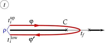
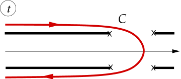
a                     b

Figure 4: (a) Contour ${\cal C}$ in the complex time plane for the calculation of the false vacuum decay probability in the in-in formalism. It supports the bounce solution in theories with unbounded scalar potential. Crosses show the branch-point singularities of the bounce. (b) Singularities of the bounce in theories with scalar potential bounded from below. The contour ${\cal C}$ must be deformed to encircle a pair of branch points.

It is now clear how to generalize this formula to an arbitrary mixed state described by a density matrix $\varrho$. To compute the decay probability, we have to average $P_{\rm true}$ with the density matrix,

$${\cal P}_{\rm decay}=\langle P_{\rm true}\rangle_{\varrho}=\int D[\varphi_{i}]D[\varphi_{i}^{\prime}]D[\varphi_{\cal C}]\,{\rm e}^{iS[\varphi_{\cal C}]}\langle\varphi_{i},t_{i}^{\rm up}|\varrho|\varphi^{\prime}_{i},t_{i}^{\rm low}\rangle\;.$$ (2.40)

In the semiclassical limit, ${\rm g}\ll 1$, the path integral can be evaluated in the saddle-point approximation. The saddle point corresponds to a solution of classical equations of motion on the contour ${\cal C}$ which we will denote by $\varphi_{\rm b}(t,x)$. It starts from the vicinity of the false vacuum at $t_{i}^{\rm up}$, evolves along the upper part of the contour to the basin of attraction of the true vacuum at $t_{f}$, and then bounces back to the false vacuum along the lower part of the contour. We refer to this solution as “bounce”. As discussed below, it provides a generalization of the Euclidean bounce describing the vacuum decay in flat spacetime [39, 40, 41].

The boundary conditions for $\varphi_{\rm b}$ at $t_{i}^{\rm up}$ and $t_{i}^{\rm low}$ are set by the density matrix $\varrho$, upon taking the saddle-point integrals in $\varphi_{i}$, $\varphi_{i}^{\prime}$. We relegate the derivation of these conditions to Appendix C. Here we present the result. When $t_{i}^{\rm up}$, $t_{i}^{\rm low}$ have large negative real part, the bounce solution linearizes and we can decompose it into the eigenmodes (2.14). At the upper part of the contour ${\cal C}$ we have

$$\varphi_{\rm b}\big{|}_{\mathop{\rm Re}\nolimits t_{i}^{\rm up}\to-\infty}=\int_{0}^{\infty}\frac{d\omega}{\sqrt{4\pi\omega}}\sum_{I=R,L}\big{[}c_{I,\omega}^{\rm up}\,\varphi_{I,\omega}^{+}(t_{i}^{\rm up},x)+\bar{c}_{I,\omega}^{\rm up}\,\varphi_{I,\omega}^{-}(t_{i}^{\rm up},x)\big{]}\;,$$ (2.41)

where $c_{I,\omega}^{\rm up}$, $\bar{c}_{I,\omega}^{\rm up}$ are constant coefficients. Similar expansion holds at the lower part of the contour for $\varphi_{\rm b}\big{|}_{\mathop{\rm Re}\nolimits t_{i}^{\rm low}\to-\infty}$ with the coefficients $c_{I,\omega}^{\rm low}$, $\bar{c}_{I,\omega}^{\rm low}$. The boundary conditions establish proportionality between the components of the upper and lower parts,

$$c_{I,\omega}^{\rm up}=r_{I}(\omega)\,c_{I,\omega}^{\rm low}~{},~{}~{}~{}~{}~{}r_{I}(\omega)\,\bar{c}_{I,\omega}^{\rm up}=\bar{c}_{I,\omega}^{\rm low}\;,$$ (2.42)

where for different vacua we have

$$r_{R}(\omega)=r_{L}(\omega)=0$$ (Boulware), (2.43a)

$$r_{R}(\omega)=r_{L}(\omega)=e^{-2\pi\omega/\lambda}$$ (Hartle–Hawking), (2.43b)

$$r_{R}(\omega)=e^{-2\pi\omega/\lambda}~{},~{}~{}~{}r_{L}(\omega)=0$$ (Unruh). (2.43c)

One can simplify these conditions by assuming that the bounce solution is unique. Then its values on the upper and lower parts of the contour must be complex conjugate,

$$\varphi_{\rm b}(t_{i}^{\rm low},x)=\varphi_{\rm b}^{*}(t_{i}^{\rm up},x)\;,$$ (2.44)

otherwise the complex conjugate configuration $\varphi_{\rm b}^{*}(t^{*},x)$ would be a different solution. This implies the relations between the frequency components, $c_{I,\omega}^{\rm low}=(\bar{c}_{I,\omega}^{\rm up})^{*}$, $\bar{c}_{I,\omega}^{\rm low}=(c_{I,\omega}^{\rm up})^{*}$, so that Eqs. (2.42) reduce to a single condition

$$c_{I,\omega}^{\rm up}=r_{I}(\omega)\,(\bar{c}_{I,\omega}^{\rm up})^{*}$$ (2.45)

imposed on the frequency components on the upper part of the contour.

We now make the following observation. Consider, instead of the tunneling probability, the generating functional for the time-ordered Green’s functions of the free theory,

$$Z[J]=\langle{\rm e}^{i(J\cdot\varphi)}\rangle_{\varrho}\;,\qquad\qquad(J\cdot\varphi)\equiv\int dtdx\sqrt{-g}\,J(t,x)\varphi(t,x)\;.$$ (2.46)

This can also be written in the in-in formalism as a path integral along the contour ${\cal C}$ from Fig. 4a,

$$Z[J]=\int D[\varphi_{i}]D[\varphi_{i}^{\prime}]D[\varphi_{\cal C}]\,{\rm e}^{iS^{(2)}[\varphi_{\cal C}]+i(J\cdot\varphi_{\cal C})}\langle\varphi_{i},t_{i}^{\rm up}|\varrho|\varphi_{i}^{\prime},t_{i}^{\rm low}\rangle\;,$$ (2.47)

where $S^{(2)}$ is the quadratic action, and the interval $(t_{i},t_{f})$ includes the support of the external source $J$. Whenever the density matrix $\varrho$ is Gaussian, the integrals are evaluated by the saddle point. The corresponding classical solution is given by a convolution of the source with the Green’s function,

$$\varphi_{J}(t,x)={\rm g}^{2}\int dt^{\prime}dx^{\prime}\mathcal{G}(t,x;t^{\prime},x^{\prime})J(t^{\prime},x^{\prime})\;.$$ (2.48)

Here the value of $\varphi_{J}$ on the lower part of the contour is obtained through the analytic continuation of the Green’s function into the lower half-plane of complex time. The asymptotic behavior of this solution at $t\to-\infty$ is determined by the saddle-point integrals over $\varphi_{i}$, $\varphi_{i}^{\prime}$. These are exactly the same as in the derivation of the boundary conditions for the bounce, implying that the boundary conditions for the bounce and for the time-ordered Green’s function coincide. Indeed, it is straightforward to check that the mode decomposition of the Green’s functions (2.32), (2.34) and (2.35) at $t\to-\infty+i\epsilon$ and $t^{\prime}$ fixed satisfies Eq. (2.45). Being real at $t=t^{\prime}$, they also satisfy the relation $\mathcal{G}(t^{*},x;t^{\prime*},x^{\prime})=\mathcal{G}^{*}(t,x;t^{\prime},x^{\prime})$, i.e., their values on the upper and lower parts of the contour ${\cal C}$ are complex conjugate to each other.

Turning the argument around, one can deduce the boundary conditions for the bounce from the asymptotics of the time-ordered Green’s function. To this aim, one just needs to find the full set of linear relations between the frequency components of the solution (2.48), which hold independently of the choice of the external source $J$. The mode decomposition of the bounce solution in the asymptotic past must then obey these relations. Note that this method is general and can be applied to tunneling from arbitrary mixed state described by a Gaussian density matrix.

The relation between the properties of the Green’s function and the bounce solution opens the following way to search for the latter. Let us split the scalar potential into the mass term $m^{2}\varphi^{2}/2$ and the interaction part $V_{\rm int}(\varphi)$. The bounce satisfies the classical field equations on the contour ${\cal C}$,

$$\Box\varphi_{\rm b}-m^{2}\Omega\varphi_{\rm b}-\Omega V^{\prime}_{\rm int}(\varphi_{\rm b})=0\;,$$ (2.49)

where prime on the potential stands for its derivative with respect to $\varphi$. This can be recast into an integral equation using the Green’s function,

$$\varphi_{\rm b}(t,x)=-i\int_{\mathcal{C}}dt^{\prime}dx^{\prime}\,\mathcal{G}(t,x;t^{\prime},x^{\prime})\,\Omega(x^{\prime})V^{\prime}_{\rm int}\big{(}\varphi_{\rm b}(t^{\prime},x^{\prime})\big{)}\;.$$ (2.50)

Taking in this expression the time-ordered Green’s function corresponding to a specific vacuum state automatically ensures the correct boundary condition for the bounce.

In general, the integral equation (2.50) is hard to solve, perhaps even harder than the boundary value problem (2.42) for the differential equation (2.49). However, there is a class of theories where the task is greatly simplified. These are theories where the nonlinear core of the bounce happens to be much smaller in size than the inverse mass $m^{-1}$. Then the source in the integral (2.50) is effectively pointlike and the solution outside the core is simply proportional to the Green’s function. On the other hand, the core of the bounce can be found by neglecting the mass. The full solution is obtained by matching the long-distance asymptotics of the core with the short-distance behavior of the Green’s function. We will encounter precisely this situation in the toy model studied later in this paper.

A few comments are in order. First, the condition (2.44) implies that the bounce solution is real at $t=t_{f}$. If $t_{f}$ is finite, the solution remains real when continued from that point along the real time axis. At $t>t_{f}$ it can be thought of as describing the evolution of the field after tunneling. On the other hand, the boundary conditions (2.45) are clearly incompatible with $\varphi_{\rm b}$, being real on the upper side of the contour ${\cal C}$. This implies that the bounce must have branch cuts in the complex time plane which the contour ${\cal C}$ must encircle [43, 52, 45, 46]. The details are somewhat different depending on whether the scalar potential is bounded or not from below, see cases (a) and (b) in Fig. 1. If the potential is unbounded, the bounce solution evolved from $t_{f}$ either forward or backward runs away to $\varphi_{\rm b}=+\infty$ in a finite time. This gives rise to singularities on the real axis shown by crosses in Fig. 4a. These singularities are also branch points and it suffices to draw the upper (lower) part of the contour ${\cal C}$ slightly above (below) the left branch cut. We will see this situation realized in our toy model. On the other hand, if the potential is bounded from below, the evolution of the scalar field along the real axis is regular. The singularities of the bounce are shifted into the complex plane. Due to the reality of the solution on the real axis, they come in complex conjugate pairs, see Fig. 4b. The contour ${\cal C}$ should then be deformed to bypass them, as shown in the figure.

Second, it may happen that the bounce solution does not exist for finite $t_{f}$. This is the case when tunneling proceeds via formation of the sphaleron, instead of a direct transition between the false and true vacua [45, 51, 69, 56, 54, 70, 63, 64, 55]. The tunneling solution can still be found if the contour ${\cal C}$ is stretched to infinity, which corresponds to $t_{f}=+\infty$. Then $\varphi_{\rm b}$ must asymptotically approach the same unstable configuration at $t\to+\infty$ along the upper and lower parts of the contour. However, because the contour actually splits into two disjoint parts, the solutions $\varphi_{\rm b}^{\rm up}$ and $\varphi_{\rm b}^{\rm low}$ need not be analytic continuations of each other. Still, their mode decompositions at $\mathop{\rm Re}\nolimits t\to-\infty$ must be related by Eqs. (2.42) and, assuming uniqueness of the bounce solution, they must be complex conjugate, $\varphi_{\rm b}^{\rm low}(t,x)=(\varphi_{\rm b}^{\rm up}(t^{*},x))^{*}$. We will see that bounce solutions of this type describe false vacuum decay at high temperatures, both in flat spacetime and in the BH background. They correspond to the transitions usually associated with thermal jumps onto the sphaleron.

Third, the boundary conditions (2.45), as well as the reality condition (2.44) are invariant under shifts of time by a real constant. Therefore, the spectrum of perturbations around the bounce contains a zero mode associated with time translations. As usual, the presence of such mode implies that the probability (2.40) linearly grows with time [39, 40, 41]. Dividing out this growth, one obtains the tunneling rate $\varGamma$.

Last, but not least, we need to know how to calculate $\varGamma$ once the bounce solution is found. In this paper we are interested only in the exponential dependence

$$\varGamma\sim{\rm e}^{-B}\;.$$ (2.51)

From Eq. (2.40) we see that $B$ is essentially equal to the imaginary part of the bounce action along the contour ${\cal C}$, plus boundary terms coming from the initial-state density matrix. It is shown in Appendix C that the latter have the form

$$\frac{i}{2{\rm g}^{2}}\int_{-\infty}^{\infty}dx\bigg{[}\varphi_{\rm b}\frac{\partial\varphi_{\rm b}}{\partial t}\bigg{|}_{t_{i}^{\rm up}}+\varphi_{\rm b}\frac{\partial\varphi_{\rm b}}{\partial t}\bigg{|}_{t_{i}^{\rm low}}\bigg{]}.$$ (2.52)

If we integrate by parts the kinetic term in the bounce action and use the equation of motion (2.49), the quadratic part of the action and the boundary terms cancel out. We end up with

$$B=-\frac{i}{{\rm\text{g}}^{2}}\int_{\mathcal{C}}dt\int_{-\infty}^{\infty}dx\;\Omega(x)\bigg{[}\frac{1}{2}\varphi_{\rm b}V^{\prime}_{\rm int}(\varphi_{\rm b})-V_{\rm int}(\varphi_{\rm b})\bigg{]},$$ (2.53)

where the time integral is taken along the contour ${\cal C}$. In this form it is manifest that only the region where the bounce solution is nonlinear contributes to the suppression.

3 Inverted Liouville potential with a mass term

In the rest of the paper we illustrate the general formalism of the previous section in a toy model with the scalar potential

$$V(\varphi)=\frac{m^{2}\varphi^{2}}{2}-2\kappa({\rm e}^{\varphi}-1)\;,$$ (3.1)

where $m^{2},\kappa>0$. The interaction term represents an inverted Liouville potential and is unbounded from below. The mass term ensures existence of a local minimum (false vacuum) at $\varphi=0$. The constant piece is chosen in such a way that $V(0)=0$. The potential is shown in Fig. 5. We assume that the parameters $m$ and $\kappa$ obey the hierarchy $m\gg\sqrt{\kappa}$ and, moreover, that the logarithm of their ratio is large,

$$\mathop{\rm ln}\nolimits\dfrac{m}{\sqrt{\kappa}}\gg 1\;.$$ (3.2)

This technical assumption will be crucial for analytic construction of the relevant semiclassical solutions.

The potential has local maximum at

$$\varphi_{\rm max}\approx\mathop{\rm ln}\nolimits{\frac{m^{2}}{2\kappa}}+\mathop{\rm ln}\nolimits{\mathop{\rm ln}\nolimits{\frac{m^{2}}{2\kappa}}}~{},~{}~{}~{}~{}~{}~{}V(\varphi_{\rm max})\approx 2m^{2}\mathop{\rm ln}\nolimits^{2}\frac{m}{\sqrt{\kappa}}\;,$$ (3.3)

where we evaluated $\varphi_{\rm max}$ up to doubly logarithmic corrections, whereas $V(\varphi_{\rm max})$ is calculated in the leading-log approximation. Above $\varphi_{\rm max}$, the potential quickly drops down and at $\varphi>\varphi_{1}\approx\mathop{\rm ln}\nolimits{\frac{m^{2}}{4\kappa}}+2\mathop{\rm ln}\nolimits{\mathop{\rm ln}\nolimits{\frac{m^{2}}{4\kappa}}}$ it becomes negative. Note that $\varphi_{1}$ differs from $\varphi_{\rm max}$ only by the doubly logarithmic terms. Thanks to the hierarchy (3.2), the theory possesses two intrinsic energy scales: the mass scale $m$ and the scale associated with the barrier $m\mathop{\rm ln}\nolimits\frac{m}{\sqrt{\kappa}}$. Both will play an important role in the studies of tunneling solutions in different environments.

Figure 5: The toy model potential.

We start by studying the dynamics of the model in flat spacetime. The equation of motion reads,

$$\Box\varphi-m^{2}\varphi+2\kappa\,{\rm e}^{\varphi}=0\;.$$ (3.4)

For large $\varphi\gtrsim\varphi_{\rm max}$ one can neglect the mass term and the equation reduces to the Liouville equation which has a general solution

$$\varphi=\mathop{\rm ln}\nolimits\bigg{[}\frac{4F^{\prime}(-u)G^{\prime}(v)}{\big{(}1+\kappa F(-u)G(v)\big{)}^{2}}\bigg{]}\;,$$ (3.5)

where $u$, $v$ are the advanced and retarded coordinates (2.10), $F(-u)$, $G(v)$ are arbitrary functions, and primes stand for the derivatives of these functions with respect to their arguments. On the other hand, at $\varphi\lesssim\varphi_{\rm max}$ the mass term dominates and the solution is the same as for the free massive theory. To find the solution of the full Eq. (3.4), we adopt the strategy of asymptotic expansion and matching. We will look for solutions in the form (3.5) (in the form of a free massive field) in the region where the second (third) term in (3.4) can be neglected. These two forms of solution will be patched together in the overlapping region where they are both valid. The condition (3.2) will be instrumental to ensure that such overlap region exists.

We now consider several solutions relevant for the false vacuum decay.

3.1 Sphaleron

Let us find the static unstable solution of Eq. (3.4) — the sphaleron $\varphi_{\rm sph}$. This solution can decay either to the true or to the false vacuum, so it can be thought of as sitting on the saddle of the potential energy functional separating the two vacua. The sphaleron energy gives the height of the energy barrier between the vacua.

Without loss of generality, we can place the center of the sphaleron at $x=0$. Then in the region $|x|\ll m^{-1}$ we can neglect the mass term and the solution reads

$$\varphi_{\rm sph}\Big{|}_{|x|\ll m^{-1}}=\mathop{\rm ln}\nolimits\bigg{[}\frac{\Lambda_{0}^{2}}{\kappa\mathop{\rm ch}\nolimits^{2}(\Lambda_{0}x)}\bigg{]}\;.$$ (3.6)

Here $\Lambda_{0}$ is a constant which must be fixed from matching with the long-distance solution. Assuming $\Lambda_{0}\gg m$, we expand (3.6) at $\Lambda_{0}^{-1}\ll|x|\ll m^{-1}$ and obtain

$$\varphi_{\rm sph}\approx-2\Lambda_{0}|x|+\mathop{\rm ln}\nolimits(4\Lambda_{0}^{2}/\kappa)\;.$$ (3.7)

On the other hand, in the outer region $|x|\gg\Lambda_{0}^{-1}$ the sphaleron is a solution to the free massive equation,

$$\varphi_{\rm sph}\Big{|}_{|x|\gg\Lambda_{0}^{-1}}=A_{\rm sph}{\rm e}^{-mx}\;,$$ (3.8)

where $A_{\rm sph}$ is another constant. At $\Lambda_{0}^{-1}\ll|x|\ll m^{-1}$ it becomes $\varphi_{\rm sph}=-A_{\rm sph}m|x|+A_{\rm sph}$. Comparing this expression with (3.7), we obtain $A_{\rm sph}=2\Lambda_{0}/m$ and an equation determining $\Lambda_{0}$,

$$\frac{\Lambda_{0}}{\mathop{\rm ln}\nolimits(2\Lambda_{0}/\sqrt{\kappa})}=m~{}~{}~{}\Longrightarrow~{}~{}~{}\Lambda_{0}=m\bigg{(}\mathop{\rm ln}\nolimits{\frac{2m}{\sqrt{\kappa}}}+\mathop{\rm ln}\nolimits\mathop{\rm ln}\nolimits{\frac{2m}{\sqrt{\kappa}}}+\ldots\bigg{)}\;.$$ (3.9)

We see that under the condition (3.2) our assumption $\Lambda_{0}\gg m$ is indeed justified. Note that the sphaleron has the following structure: a narrow nonlinear core of the size $\Lambda_{0}^{-1}$, where the field reaches $\varphi_{\rm sph}\sim\varphi_{1}$, and a wide tail (3.8), where the field is linear. This structure will be recurrent in the other semiclassical solutions that we consider below.

To calculate the sphaleron energy, it is convenient to integrate by parts the gradient term in the standard expression for the energy and use the equation of motion. This yields (up to a negligible contribution of order $\mathcal{O}(\kappa/m)$)

$$E_{\rm sph}=\frac{1}{{\rm\text{g}}^{2}}\int_{-\infty}^{\infty}dx\,\kappa\,(\varphi_{\rm sph}-2)\,{\rm e}^{\varphi_{\rm sph}}\;.$$ (3.10)

The integral is saturated by the nonlinear core and substituting Eq. (3.6), we obtain

$$E_{\rm sph}=\frac{4\Lambda_{0}}{{\rm\text{g}}^{2}}\bigg{(}\mathop{\rm ln}\nolimits\frac{\Lambda_{0}}{\sqrt{\kappa}}-2+\mathop{\rm ln}\nolimits{2}\bigg{)}\approx\frac{4m}{{\rm\text{g}}^{2}}\bigg{(}\mathop{\rm ln}\nolimits\frac{m}{\sqrt{\kappa}}\bigg{)}^{2}\;,$$ (3.11)

where the last expression is written in the leading-log approximation. Notice that the sphaleron energy is doubly enhanced: by the inverse of the small coupling constant g and by the large logarithm $\mathop{\rm ln}\nolimits(m/\sqrt{\kappa})$.

3.2 Tunneling from Minkowski vacuum

Next, we consider the bounce solution describing the false vacuum decay in empty Minkowski spacetime. We first adopt the standard Euclidean approach and then show how it is related to the in-in method developed in Sec. 2.

In the standard approach, the bounce represents a saddle point of the Euclidean partition function [39, 40, 41]. It is a solution of the field equations obtained upon Wick rotation of the time variable to purely imaginary values, $t\mapsto-i\tau$. The solution $\varphi_{\rm b}$ is assumed to be real for real $\tau$, vanish at infinity, and have zero time derivative at $\tau=0$. The latter property ensures that the analytic continuation of the bounce onto the real time axis is real and describes the evolution of the field after tunneling. It is customary to assume that the bounce with the smallest Euclidean action, and hence giving the least suppressed channel for the vacuum decay, is spherically-symmetric in the Euclidean spacetime. This means that the bounce depends only on $\rho=\sqrt{x^{2}+\tau^{2}}$ and obeys the equation

$$\partial^{2}_{\rho}\varphi_{\rm b}+\frac{1}{\rho}\partial_{\rho}\varphi_{\rm b}-m^{2}\varphi_{\rm b}+2\varkappa\,{\rm e}^{\varphi_{\rm b}}=0\;.$$ (3.12)

We again use the strategy of splitting the solution into a core and a tail and matching them in the overlap. At $\rho\ll m^{-1}$ we neglect the mass term and obtain

$$\varphi_{\rm b}\Big{|}_{\rho\ll m^{-1}}=\mathop{\rm ln}\nolimits\left[\frac{4C^{2}_{M}}{(1+\kappa C_{M}^{2}\rho^{2})^{2}}\right]\;,$$ (3.13)

where $C_{M}$ is a constant. This corresponds to the following choice of linear functions $F$, $G$ in the general solution (3.5):

$$F(z)=C_{M}\,z\;,~{}~{}~{}G(\bar{z})=C_{M}\,\bar{z}\;,$$ (3.14)

where we have adapted the notations to the Euclidean signature,

$$-u\mapsto z=x+i\tau\;,~{}~{}~{}~{}v\mapsto\bar{z}=x-i\tau\;.$$ (3.15)

At $(C_{M}\sqrt{\kappa})^{-1}\ll\rho\ll m^{-1}$ the core solution becomes

$$\varphi_{\rm b}\approx-4\mathop{\rm ln}\nolimits(\sqrt{\kappa}\rho)-2\mathop{\rm ln}\nolimits C_{M}+2\mathop{\rm ln}\nolimits 2\;.$$ (3.16)

On the other hand, the tail is given by the solution of the free massive equation,

$$\varphi_{\rm b}\Big{|}_{\rho\gg(C_{M}\sqrt{\kappa})^{-1}}=A_{M}K_{0}\left(m\rho\right)\;,$$ (3.17)

where $K_{0}$ is the modified Bessel function of the second kind and $A_{M}$ is another constant. Expansion at small $\rho$ gives $\varphi_{\rm b}\approx-A_{M}\mathop{\rm ln}\nolimits(m\rho)+A_{M}(\mathop{\rm ln}\nolimits 2-\gamma_{E})$, where $\gamma_{E}$ is the Euler constant. Comparing with Eq. (3.16), we obtain $A_{M}=4$ and

$$C_{M}=\frac{m^{2}}{2\kappa}{\rm e}^{2\gamma_{E}}\;.$$ (3.18)

We can now verify a posteriori that the matching region exists. The condition is $C_{M}\sqrt{\kappa}\gg m$, which is indeed implied by our assumption (3.2).

Let us see how the above results are reproduced by the method of Sec. 2. We notice that the core of the solution (3.13) is an analytic function of complex time with branch-cut singularities on the real axis at

$$t=\pm t_{M,s}(x)~{},~{}~{}~{}~{}t_{M,s}(x)=\sqrt{x^{2}+(C_{M}\sqrt{\kappa})^{-1}}\;.$$ (3.19)

Further, the tail of the solution (3.17) is proportional to the analytic continuation to the Euclidean time of the Feynman Green’s function

$$\mathcal{G}_{F}(t,x;0,0)=\frac{1}{2\pi}K_{0}\left(m\sqrt{x^{2}-t^{2}+i\epsilon}\right)\;.$$ (3.20)

This implies that the bounce solution can be analytically continued to the whole complex plane of $t$ with only singularities at (3.19), see Fig. 6. In particular, it is defined on the contour ${\cal C}$ introduced in Sec. 2.4. Moreover, at the endpoints of this contour it obeys the Feynman boundary conditions, as required for the tunneling from vacuum. We conclude that for the problem at hand the tunneling solution given by the method of Sec. 2.4 and the standard Euclidean bounce are just different representations of the same analytic function — simply stated, they coincide.

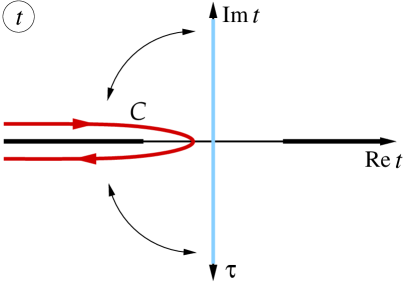
Figure 6: Structure of Minkowski bounce in the complex time plane. The standard Euclidean bounce is defined on the imaginary time axis (blue). Its analytic continuation to the contour ${\cal C}$ (red) satisfies Feynman boundary conditions at $\mathop{\rm Re}\nolimits t\to-\infty$. Thick black lines show the branch cuts.

The singularity of the bounce solution at $t>0$ has a natural physical interpretation. It corresponds to the run-away of the field towards $\varphi=+\infty$ after tunneling. We observe that it is mirrored by a twin singularity at $t<0$. The latter does not appear to have any transparent physical meaning. However, as discussed in Sec. 2.4, its presence is necessary for existence of a nontrivial tunneling solution on the contour ${\cal C}$.

To compute the tunneling suppression, we can either integrate the bounce action in the Euclidean time, as in the standard approach, or use the integral (2.53) along the contour ${\cal C}$. The two results will coincide, because we can continuously deform the contour ${\cal C}$ into the imaginary time axis, and vice versa, see Fig. 6. Notice that the integrals along the arcs at infinity vanish. Indeed, at $|t|\to\infty$, $\mathop{\rm Im}\nolimits t\neq 0$ the field linearizes and does not contribute into the tunneling suppression, as is clear from the expression (2.53). The result reads

$$B_{M}=\frac{16\pi}{{\rm\text{g}}^{2}}\bigg{(}\mathop{\rm ln}\nolimits\frac{m}{\sqrt{\kappa}}+\gamma_{E}-1\bigg{)}\;.$$ (3.21)

We observe that the suppression is enhanced by the large logarithm (3.2). This contribution can be traced back to the large value of the field at the core of the bounce $\varphi_{\rm b}(0)=4\big{(}\mathop{\rm ln}\nolimits(m/\sqrt{\kappa})+\gamma_{E}\big{)}$. It is easily computed by replacing the field in the integral for $B$, when it appears outside the exponent, by its value at the core and taking the resulting integral with residues,

$$\begin{split}B_{M}\Big{|}_{\rm leading-log}&=\frac{i}{{\rm g}^{2}}\int_{\cal C}dt\int_{-\infty}^{\infty}dx\,\kappa\,\varphi_{\rm b}(0)\,{\rm e}^{\varphi_{\rm b}(t,x)}\\ &=\frac{2\pi\varphi_{\rm b}(0)}{{\rm g}^{2}}\int_{-\infty}^{\infty}dx\,\kappa\,\mathop{\mathrm{Res}}_{t=-t_{M,s}(x)}{\rm e}^{\varphi_{\rm b}(t,x)}=\frac{4\pi}{{\rm g}^{2}}\varphi_{\rm b}(0)\;.\end{split}$$ (3.22)

One can use this replacement to quickly get the leading-log contribution to the suppression in the cases when the full calculation may be complicated.

3.3 Thermal transitions in flat spacetime

Here we study false vacuum decay in flat spacetime at finite temperature. The results of this section will be important in what follows for the analysis of instanton solutions in the Hartle–Hawking and Unruh vacua. To make contact with those cases, we denote the temperature by $\lambda/(2\pi)$ and assume $\lambda$ to be much larger than $m$.

We again begin with the standard approach which prescribes to look for a real solution of the Euclidean field equation periodic in Euclidean time $\tau$ with the period $2\pi/\lambda$. This periodic instanton is the saddle point of the thermal partition function. We make an educated guess for the functions $F$ and $G$ describing the core of the instanton,

$$F(z)=\dfrac{C_{th}}{\lambda}\left({\rm e}^{\lambda z}-d_{th}\right)\;,~{}~{}~{}~{}~{}G(\bar{z})=\dfrac{C_{th}}{\lambda}\left({\rm e}^{\lambda\bar{z}}-d_{th}\right)\;,$$ (3.23)

with real constants $C_{th}$, $d_{th}$. Substituting into the expression for the field (3.5), after some elementary manipulations we obtain

$$\varphi_{\rm b}\Big{|}_{\rm core}=\mathop{\rm ln}\nolimits\left[\frac{\lambda^{2}b_{th}}{\kappa\left(\mathop{\rm ch}\nolimits\lambda x-\sqrt{1-b_{th}}\cos\lambda\tau\right)^{2}}\right]\;,$$ (3.24)

where we have denoted

$$b_{th}=\frac{\lambda^{2}}{\kappa C^{2}_{th}}$$ (3.25)

and have placed the center of the instanton at $x=0$ by setting $d_{th}=\sqrt{1-b_{th}}$. We have provisionally denoted the solution as $\varphi_{\rm b}$, and we will see shortly that it indeed describes the bounce in the sense of Sec. 2.4. The solution is real as long as $b_{th}<1$.

Let us first assume that $b_{th}\ll 1$. Then at $|x|,|\tau|\gtrsim 1/\lambda$ the solution becomes

$$\varphi_{\rm b}\approx-2\mathop{\rm ln}\nolimits\left[4\mathop{\rm sh}\nolimits\bigg{(}\frac{\lambda z}{2}\bigg{)}\mathop{\rm sh}\nolimits\bigg{(}\frac{\lambda\bar{z}}{2}\bigg{)}\right]+\mathop{\rm ln}\nolimits\left[\frac{4\lambda^{2}b_{th}}{\kappa}\right]\;.$$ (3.26)

This has the same form as the Wick rotated thermal Green’s function when its two arguments are separated by less than $1/m$ (“close separation”), see Eq. (B.32). Thus, the tail of the instanton is given by this Green’s function,

$$\varphi_{\rm b}\Big{|}_{\rm tail}=8\pi\mathcal{G}_{th}(-i\tau,x;0,0)\;,$$ (3.27)

where the proportionality coefficient has been fixed by matching the singular part of $\mathcal{G}_{th}$. Comparing the constant pieces in (3.26) and (B.32), we fix

$$b_{th}=\frac{\kappa}{4\lambda^{2}}{\rm e}^{\frac{2\lambda}{m}}\;,$$ (3.28)

which is indeed small if the temperature does not exceed a certain critical value. It is easy to see that the latter coincides with $\Lambda_{0}$ determined by Eq. (3.9).

This is not an accident: when $\lambda$ approaches $\Lambda_{0}$ and $b_{th}$ approaches $1$, the periodic instanton becomes $\tau$-independent and degenerates into the sphaleron. The matching procedure used above becomes problematic in this limit and fails to describe this transition since the region where the instanton can be written in the form (3.26) seizes to exist in Euclidean time (we will see shortly how to remedy this problem). Still, the transition of periodic instantons into the sphaleron is expected on general grounds. It is well-known that in field theory at high temperature there are no nontrivial periodic instantons and the false vacuum decay proceeds by thermal jumps over the barrier separating it from the true vacuum [74]. The probability of the latter process is suppressed by the Boltzmann exponent involving the height of the barrier, i.e., the sphaleron energy, divided by the temperature, $\Gamma\sim\exp(-2\pi E_{\rm sph}/\lambda)$. Alternatively, the suppression can be obtained as the sphaleron action over the Euclidean time interval $2\pi/\lambda$.

Let us now reinterpret the above results along the lines of Sec. 2. Periodic instanton (3.24) is an analytic function of complex time with branch cuts on the real axis starting at

$$t=\pm t_{th,s}(x)~{},~{}~{}~{}~{}t_{th,s}(x)=\frac{1}{\lambda}\mathop{\rm arcch}\nolimits\left(\frac{\mathop{\rm ch}\nolimits\lambda x}{\sqrt{1-b_{th}}}\right)\;,$$ (3.29)

see Fig. 7a. This structure is similar to that of the vacuum Minkowski bounce (cf. Fig. 6). The singularity at $t>0$ corresponds to the run-away of the field after tunneling. On the other hand, the branch cut at $t<0$ ensures the correct asymptotics of the solution along the contour ${\cal C}$. Indeed, in the far past the solution linearizes and coincides with the thermal Green’s function, see Eq. (3.27). Therefore, its mode decomposition on the upper part of the contour (2.41) satisfies the relations (2.42) with the thermal coefficient (2.43b). Thus, the periodic instanton, analytically continued onto the contour ${\cal C}$, satisfies all the requirements on the bounce solution formulated in Sec. 2.4.

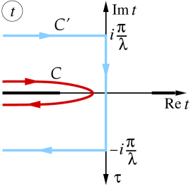
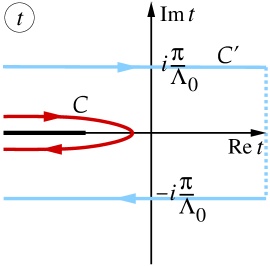
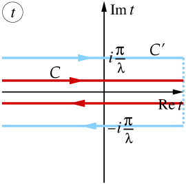
a               b                c

Figure 7: Structure of the thermal bounce in the complex time plane. (a) Low temperature solutions at $\lambda<\Lambda_{0}$ correspond to periodic instantons in Euclidean time. At real $t>0$ they describe run-away of the field $\varphi$ to the true vacuum at $\varphi=+\infty$. (b) The bounce solution at $\lambda=\Lambda_{0}$ tends to the sphaleron at $\mathop{\rm Re}\nolimits t\to+\infty$. (c) Solutions at $\lambda>\Lambda_{0}$ describe tunneling onto the sphaleron. They are given by different analytic functions on the upper and lower parts of the contour ${\cal C}$ that runs from $t=-\infty$ to $t=+\infty$ and backward. See the text for more details.

The corresponding tunneling suppression can be computed along the contour ${\cal C}$. It is convenient, however, to deform the latter into the contour ${\cal C}^{\prime}$ shown with blue in Fig. 7a. Due to the periodicity of $\varphi_{\rm b}$ in complex time, the integrals over the parts of this contour at $\mathop{\rm Im}\nolimits t=\pm\pi/\lambda$ cancel each other and we are left with the contribution along the portion of the imaginary time axis from $t=i\pi/\lambda$ to $t=-i\pi/\lambda$. This is nothing but the Euclidean action of the periodic instanton over a single period. We evaluate it in Appendix D with the result

$$B_{th}=\dfrac{16\pi}{\text{g}^{2}}\left(\mathop{\rm ln}\nolimits\dfrac{\lambda}{\sqrt{\kappa}}-\dfrac{\lambda}{2m}+\mathop{\rm ln}\nolimits 2-1\right)~{},~{}~{}~{}~{}~{}\lambda<\Lambda_{0}\;.$$ (3.30)

Notice that for $\lambda\sim m$ we recover the vacuum suppression (3.21) in the leading-log approximation. The $\mathcal{O}(1)$-terms are different, because in deriving (3.30) we used the assumption $\lambda\gg m$.

When $b_{th}\to 1$, i.e., when we approach the sphaleron regime, the singularities (3.29) move away from the origin and at $b_{th}=1$ run to infinity. One may be puzzled how one can obtain a bounce solution with correct asymptotics in this case, given that the sphaleron is time-independent and thus never linearizes. The answer is simple: one just needs to slightly modify the limit by shifting the periodic instanton in time in such a way that the left singularity is kept at a finite distance. Namely, one makes a replacement

$$t\mapsto t+\frac{1}{2\lambda}\mathop{\rm ln}\nolimits(1-b_{th})\;,$$ (3.31)

so that the core solution (3.24) becomes

$$\varphi_{\rm b}\Big{|}_{\rm core}=\mathop{\rm ln}\nolimits\bigg{[}\frac{\lambda^{2}b_{th}}{\kappa\left(\mathop{\rm ch}\nolimits\lambda x-\tfrac{1}{2}{\rm e}^{-\lambda t}-\tfrac{1}{2}(1-b_{th}){\rm e}^{\lambda t}\right)^{2}}\bigg{]}\;.$$ (3.32)

This can now be matched to the tail (3.27) at $\mathop{\rm Re}\nolimits t<0$ for any values of $b_{th}$, not necessarily small. The matching is performed in the region $\mathop{\rm Re}\nolimits t<0$; $\lambda^{-1}\ll|\mathop{\rm Re}\nolimits t|$; $|t|,|x|\ll m^{-1}$. In this region the coefficient of the term ${\rm e}^{\lambda t}$ in Eq. (3.32) is irrelevant. If we set it to $1/2$, we recover the form of the Green’s function at close separation, Eq. (B.32). Matching the constant parts of $\varphi_{\rm b}\big{|}_{\rm core}$ and $\varphi_{\rm b}\big{|}_{\rm tail}$ reproduces Eq. (3.28) for $b_{th}$, which is now valid for any $b_{th}\leq 1$.

Importantly, when $b_{th}=1$ the solution (3.32) still linearizes at $\mathop{\rm Re}\nolimits t\to-\infty$ and obeys the boundary conditions appropriate for tunneling from a thermal state with temperature $\Lambda_{0}$. The solution does not have singularities at $\mathop{\rm Re}\nolimits t>0$, thus it does not directly interpolate to the true vacuum (see Fig. 7b). Instead, at $\mathop{\rm Re}\nolimits t\to+\infty$ it asymptotically tends to the sphaleron, approaching it along the unstable direction. This phenomenon can be called “tunneling onto the sphaleron” and has been previously observed in the context of semiclassical transitions induced by particle collisions [51, 54, 56, 55] and in quantum mechanics with multiple degrees of freedom [45, 69, 70, 63, 64]. The sphaleron formed in this way later decays into the true vacuum with order-one probability, therefore, all exponential suppression comes from the first stage of the process — formation of the sphaleron — which is captured by the semiclassical solution.

What is the structure of the bounce at $\lambda>\Lambda_{0}$? Naively, one could think that it is given by the continuation of the expression (3.32) to $b_{th}>1$. However, this does not work: it is straightforward to see that the resulting configurations decay back to the false vacuum at $t>0$ and thus do not describe appropriate transitions. The true bounce solution is still expected to tunnel on top of the sphaleron. However, at this temperature there is no single analytic function that would be a solution of the field equations, satisfy the boundary conditions (2.42), (2.43b) at $\mathop{\rm Re}\nolimits t\to-\infty$, and approach the sphaleron at $\mathop{\rm Re}\nolimits t\to+\infty$. We are in the regime discussed at the end of Sec. 2.4 when the bounce cannot be found on a contour ${\cal C}$ with a finite turn-around point $t_{f}$. However, we can still construct the solution if we pull the turn-around point to infinity as in Fig. 7c. In this case the solution on the upper and lower halves of the contour need not be the same analytic function, the only requirement being that they have the same limit at $\mathop{\rm Re}\nolimits t\to+\infty$. It is straightforward to see that the following Ansatz will do the job:

$$\begin{split}&\varphi_{\rm b}^{\rm up}(t,x)=\varphi_{\rm b}^{(\Lambda_{0})}\left(t+i\pi\big{(}\tfrac{1}{\Lambda_{0}}-\tfrac{1}{\lambda}\big{)},x\right)\;,\\ &\varphi_{\rm b}^{\rm low}(t,x)=\varphi_{\rm b}^{(\Lambda_{0})}\left(t-i\pi\big{(}\tfrac{1}{\Lambda_{0}}-\tfrac{1}{\lambda}\big{)},x\right)\;,\end{split}$$ (3.33)

where $\varphi_{\rm b}^{(\Lambda_{0})}$ is the bounce solution for the critical temperature $\lambda=\Lambda_{0}$.

The corresponding tunneling suppression can be evaluated along the contour ${\cal C}$. It is simpler, however, to deform it into the contour ${\cal C}^{\prime}$ as shown in Figs. 7b,c. The integrals over the upper and lower halves of the contour cancel due to the periodicity of $\varphi_{\rm b}^{(\Lambda_{0})}$, and the only remaining contribution comes from the piece at $\mathop{\rm Re}\nolimits t=+\infty$ (shown with dashed lines in the figure). The solution there simply coincides with the static sphaleron and the suppression is given by its energy times the difference in the imaginary time between the upper and lower parts of the contour,

$$B_{th}=\frac{2\pi E_{\rm sph}}{\lambda}~{},~{}~{}~{}~{}~{}\lambda\geq\Lambda_{0}\;.$$ (3.34)

Thus, we have recovered with the in-in formalism of Sec. 2 the standard high-energy transition rate associated with jumps over the potential barrier.

Recalling the formula for the sphaleron energy (3.11), we see that at $\lambda=\Lambda_{0}$ the two expressions (3.30), (3.34) smoothly match, up to the first derivative with respect to $\lambda$, whereas the second derivative is discontinuous. At the matching point the suppression is roughly equal to half the suppression of the vacuum tunneling (3.21). These findings are summarized in Fig. 8.

Figure 8: Tunneling suppression $B_{th}$ in flat spacetime at different temperatures $\lambda/(2\pi)$. Dashed line represents the decay channel via the sphaleron. The change to sphaleron dominated transitions occurs at $\Lambda_{0}$ given by Eq. (3.9). $B_{M}$ represents suppression in empty space, Eq. (3.21).

Finally, let us make an observation which will be useful later, when studying decay of the Unruh vacuum. The leading term in the suppression of transitions at high temperature can be found with a different method. When $\lambda/(2\pi)\gg m$, the occupation numbers of modes with $\omega\sim m$ are large. Hence, $\varphi$ can be viewed as a classical stochastic field. The low-frequency modes dominate thermal field fluctuations. Their variance is found from the thermal Green’s function at coincident points, upon renormalizing it by subtraction of the Green’s function in empty space,

$$\delta\varphi_{th}^{2}=\text{g}^{2}\lim_{t,x\to 0}\big{[}\mathcal{G}_{th}(t,x;0,0)-\mathcal{G}_{F}(t,x;0,0)\big{]}\approx\frac{{\rm g}^{2}\lambda}{4\pi m}\;,$$ (3.35)

where we have used Eqs. (B.14), (B.32). Now we can estimate the transition probability as the probability of the field fluctuation reaching beyond the maximum of the potential barrier $\varphi_{\rm max}$. Since the interaction quickly dies out at $\varphi<\varphi_{\rm max}$, we can take the fluctuations to be Gaussian, so that

$$\varGamma_{\text{high-}\lambda}\sim\exp\left(-\frac{\varphi_{\rm max}^{2}}{2\,\delta\varphi_{th}^{2}}\right)\sim\exp\left[-\frac{8\pi m}{{\rm g}^{2}\lambda}\left(\mathop{\rm ln}\nolimits\frac{m}{\sqrt{\kappa}}\right)^{2}\right]\;,$$ (3.36)

where we used the leading term in the expression (3.3) for $\varphi_{\rm max}$. This coincides with the leading-log part of the exact high-temperature suppression (3.34).

It is worth stressing that the possibility to make the simple estimate (3.36) hinges on two peculiar properties of our model. The first is the dominance of the field fluctuations by long modes with wavelengths of order $1/m$, which is due to the two-dimensional nature of the model. Thanks to this property, the field changes coherently in large regions of space, comparable to the size of the sphaleron. The second property is the abrupt variation of the scalar potential around $\varphi_{\rm max}$, which implies that the field is essentially linear at $\varphi<\varphi_{\rm max}$, whereas almost any fluctuation towards $\varphi>\varphi_{\rm max}$ leads to a roll-over of the field into the true vacuum. In principle, the stochastic approach can also work in more general situations, but will require full-fledged simulations of the classical field dynamics to determine the vacuum decay rate [75, 76, 77, 78].

4 Minkowski bounce as periodic instanton in Rindler space

Rindler spacetime presents the simplest example of a nontrivial metric to test our approach. It corresponds to the line element (2.5) with

$$\Omega={\rm e}^{2\lambda x}\;.$$ (4.1)

The curvature of spacetime is still zero,

$$R=-\Omega^{-1}\Box\mathop{\rm ln}\nolimits\Omega=0\;,$$ (4.2)

and the change of variables

$$T=\lambda^{-1}{\rm e}^{\lambda x}\mathop{\rm sh}\nolimits\lambda t\;,~{}~{}~{}~{}~{}X=\lambda^{-1}{\rm e}^{\lambda x}\mathop{\rm ch}\nolimits\lambda t$$ (4.3)

brings the line element to the Minkowski form $ds^{2}=-dT^{2}+dX^{2}$. The original coordinates $(t,x)$ cover the right wedge of Minkowski space $X>|T|$. The lines of constant $x$ represent trajectories of uniformly accelerated observers with the acceleration $\lambda{\rm e}^{-\lambda x}$. Note that the acceleration decreases at large $x$. The time variable $t$ is the proper time of the observer at $x=0$. While Rindler space is interesting on its own right, for us it has an additional value since it describes the near-horizon region of a BH, as it is clear from Eq. (2.6). Thus, understanding the bounce solutions in the Rindler geometry will give us insight about tunneling in BH background.

The field equation now reads

$$\Box\varphi-m^{2}\,\Omega\,\varphi+2\kappa\,\Omega\,{\rm e}^{\varphi}=0\;.$$ (4.4)

If we neglect the mass term, it is still exactly solvable due to the property (4.2) with the general solution

$$\varphi=\mathop{\rm ln}\nolimits\left[\frac{4F^{\prime}(-u)G^{\prime}(v)}{\Omega(u,v)\big{(}1+\kappa F(-u)G(v)\big{)}^{2}}\right]\;.$$ (4.5)

This is, of course, a consequence of the solvability of the Liouville equation in flat spacetime.

The complete set of Rindler mode functions is given by Eq. (B.9) from the Appendix. Due to the unbounded growth of the effective potential in the mode equation (2.15), all modes quickly vanish at $x\to+\infty$. At $x\to-\infty$ they represent the sum of right- and left-moving waves with equal amplitudes. This means that, unlike flat or BH background, there is no separation into left- and right-moving modes. In particular, in Rindler space there is no analog of the Unruh vacuum which requires different occupation of left and right modes.

On the other hand, an analog of the Hartle–Hawking state does exist and is given by the Minkowski vacuum. We focus on tunneling from this state. In principle, one can find the bounce directly in the coordinates $(t,x)$ by using an appropriate Ansatz for the core and matching it to the Green’s function at the tail. We do not need to do it, however, because we already know the form of the bounce in flat spacetime, Eqs. (3.13), (3.17). We consider a bounce centered at a point $(\mathcal{T}=0,X=X_{0})$ in flat Euclidean space, with $\mathcal{T}=iT$. Then replacing $\rho$ in Eq. (3.13) by $\sqrt{\mathcal{T}^{2}+(X-X_{0})^{2}}$ and performing the Euclidean version of the coordinate change (4.3),

$$\mathcal{T}=\lambda^{-1}{\rm e}^{\lambda x}\sin{\lambda\tau}~{},~{}~{}~{}~{}~{}X=\lambda^{-1}{\rm e}^{\lambda x}\cos{\lambda\tau}\;,$$ (4.6)

we obtain in the Rindler frame

$$\varphi_{\rm b}\Big{|}_{\text{core}}=\mathop{\rm ln}\nolimits\left[\dfrac{\lambda^{2}b_{R}}{\kappa\left(\mathop{\rm ch}\nolimits\lambda(x-x_{0})\mp\sqrt{1-b_{R}}\cos\lambda\tau\right)^{2}}\right]-2\lambda x\;.$$ (4.7)

Here

$$x_{0}=\frac{1}{2\lambda}\mathop{\rm ln}\nolimits\left[\frac{\lambda^{2}}{\kappa C^{2}_{M}}+\lambda^{2}X_{0}^{2}\right]~{},~{}~{}~{}~{}~{}~{}b_{R}=\frac{\lambda^{2}}{\kappa C^{2}_{M}}{\rm e}^{-2\lambda x_{0}}\;,$$ (4.8)

and the minus (plus) sign corresponds to $X_{0}>0$ ($X_{0}<0$). Similar transformations with Eq. (3.17) give

$$\varphi_{\rm b}\Big{|}_{\text{tail}}=4K_{0}\left(\frac{m}{\lambda}\sqrt{{\rm e}^{2\lambda x}\mp 2\sqrt{1-b_{R}}\,{\rm e}^{\lambda(x+x_{0})}\cos\lambda\tau+(1-b_{R}){\rm e}^{2\lambda x_{0}}}\right)\;.$$ (4.9)

We first focus on the solutions with the minus sign in Eqs. (4.7), (4.9). We observe that the core solution (4.7) is the same as the core of the periodic instanton in flat space, Eq. (3.24), up to a linear term that comes from the factor $\Omega^{-1}(x)$ inside the logarithm in the general solution (4.5). Thus, the flat-space vacuum bounce in Cartesian coordinates becomes a periodic instanton in the Rindler frame. This is what one expects because the Minkowski vacuum corresponds to a thermal state from the viewpoint of an accelerated observer [66].

The physical temperature seen by observers at different positions $x$ is, however, different due to the redshift introduced by the space-dependent metric. The Green’s function probes the field nonlocally and is sensitive to this deviation from equithermality. As a consequence, the tail of the Rindler bounce (4.9) is not the same as in the flat-space periodic instanton. To see this explicitly, let us expand the tail (4.9) in the region where the argument of the Bessel function is small. Assuming for simplicity $b_{R}\ll 1$, we obtain

$$\varphi_{\rm b}\approx-2\mathop{\rm ln}\nolimits\left[4\mathop{\rm sh}\nolimits\left(\frac{\lambda z}{2}\right)\mathop{\rm sh}\nolimits\left(\frac{\lambda\bar{z}}{2}\right)\right]-2\lambda x-2\lambda x_{0}+4\mathop{\rm ln}\nolimits\frac{\lambda}{m}+4\mathop{\rm ln}\nolimits 2-4\gamma_{E}\;.$$ (4.10)

This must be contrasted with the flat-space thermal Green’s function at close separation, Eq. (B.32). We see that while the singular parts of the two expressions are proportional to each other, the constants have different dependence on $\lambda/m$. Furthermore, the expression (4.10) contains a linear-in-$x$ piece, which is absent from (B.32). It matches a similar linear piece in the core solution (4.7). Different constant in Eqs. (4.10), (B.32) lead to different expressions for the parameter $b$, cf. Eqs. (3.28), (4.8). This, in turn, translates into different tunneling suppressions, see below.

Let us now discuss the choice of sign in Eqs. (4.7), (4.9). We notice that the evident freedom in choosing the center of the instanton at $X=X_{0}$ in Minkowski coordinates becomes somewhat nontrivial when expressed in terms of $(\tau,x)$. For different values of $X_{0}$, the solutions (4.7) on the real positive time axis describe different dynamics of a true vacuum region (see Fig. 9):

• $X_{0}>0$ (negative sign in Eqs. (4.7), (4.9)). In Cartesian coordinates, $\varphi_{\rm b}$ is a vacuum bounce shifted to the right with respect to the origin. On the real positive time axis $t$, $\varphi_{b}$ describes a bubble of true vacuum expanding outwards the horizon.

• $X_{0}=0$. Then $b_{R}=1$ and $\varphi_{\rm b}$ becomes $\tau$-independent. It represents the sphaleron of Rindler observers. In Cartesian coordinates this sphaleron is a flat vacuum bounce sitting symmetrically around the origin $X=0$.

• $X_{0}<0$ (positive sign in Eqs. (4.7), (4.9)). In Cartesian coordinates, $\varphi_{\rm b}$ is a vacuum bounce shifted to the left with respect to the origin. Its part in the Rindler wedge at real positive $t$ describes a bubble of true vacuum collapsing towards the horizon. This leaves the false vacuum in the Rindler wedge intact. We conclude that this branch of solutions is irrelevant for the false vacuum decay in Rindler space and should be discarded.

Figure 9: Schematic plot of the family of periodic instantons in Rindler spacetime (left) and their form in Euclidean time in Cartesian coordinates (right). Red line marks the surface at which the instanton is continued to real time. From left to right: the collapsing bubble (brown), the sphaleron (blue), the expanding bubble (green).

We draw one more lesson from the above discussion. Although the Rindler metric is not homogeneous, there is still a freedom in choosing the center of the instanton $x_{0}$ in Eq. (4.7), corresponding to the choice of $X_{0}>0$. This is a nontrivial observation. Shifts in $X$ do not preserve the position of the horizon. Hence, they are not an isometry of the Rindler spacetime. Nevertheless, $x_{0}$ represents a zero mode of the solution. By varying $x_{0}$, the branch of periodic instantons is continuously connected to the sphaleron.

Finally, we compute the tunneling action. As usual, we take the general formula (2.53), substitute the solution in the core (4.7) and integrate over one period of oscillation in Euclidean time, $0<\tau<2\pi/\lambda$. We obtain, as we should, that the action does not depend on $x_{0}$ or $\lambda$ and coincides with the action of the flat vacuum bounce (3.21).

Two comments are in order. First, the independence of the action of the position of the instanton and of temperature might seem counter-intuitive from the viewpoint of a Rindler observer. However, it follows inevitably from the invariance of the tunneling probability under changes of the reference frame. Second, note that the Rindler observer does not have access to the portion of the Minkowski vacuum bubble hidden by the horizon. In particular, the Rindler sphaleron is only half of the Minkowski bubble on the slice $T=0$. It is this half that we use to compute the sphaleron Rindler energy and the corresponding suppression. However puzzling it might seem at first, the result we obtain coincides with the full flat-space integration. This supports the conclusion that parts of spacetime outside the physical wedge are not relevant for tunneling and one can exclude them completely from consideration.

5 Tunneling in black hole background

We are now ready to address tunneling in the BH background. The field equation has the form (4.4) with the metric function given by Eq. (2.7). Even if we neglect the mass term, this equation is not in general exactly solvable. One could try to maintain solvability by adding a coupling between the field $\varphi$ and curvature to ensure the conformal invariance of the Liouville part of the action. This path is, however, not suitable for our purposes. As discussed in Appendix E, the nonminimal coupling leads to a deformation of the classical vacuum in the presence of BH and increases the barrier between the false and true vacua. This leads to an artificial suppression of the tunneling rate, which is not present in realistic situations.

Therefore, we stick to the minimal coupling case and notice that, in the absence of mass, Eq. (4.4) can still be solved in two regions: near horizon, and far away from BH. In both these cases we have $|x|\gg 1/\lambda$ and $(\mathop{\rm ln}\nolimits\Omega)^{\prime\prime}=0$, hence the general solution is given by Eq. (4.5). This will suffice to find the bounce solutions whose cores are contained entirely in one of those regions. Notice that this does not impose any restrictions on the tails of the solutions described by the Green’s functions of the free massive theory, which can extend across the boundary between the two regions. We are going to see that the majority of bounce solutions satisfy this requirement.

In the main text we focus on the physically relevant cases of tunneling from the Hartle–Hawking and Unruh states. For completeness we also consider the Boulware vacuum in Appendix F. We find that the suppression in the latter case is essentially the same as in flat space, with only a minor enhancement due to the vacuum polarization by the gravitational field. On the other hand, the thermal excitations present in the Hartle–Hawking and Unruh vacua have a dramatic effect on the decay rate, as we presently show. Throughout this section we assume $\lambda\gg m$.

5.1 Hartle–Hawking vacuum

5.1.1 Moderate temperature: Tunneling near horizon

Let us make an assumption that tunneling is dominated by periodic instantons with the core in the near-horizon region $x<0$, $|x|\gg 1/\lambda$. We will see that this is indeed the case as long as the BH temperature does not exceed a certain critical value $\Lambda_{HH}$. We will work in the Euclidean signature to make contact with previous studies and refer the reader to Sec. 3.3 for the discussion of the relation to the in-in formalism. We make the thermal Ansatz for the functions parameterizing the solution in the core (cf. Eq. (3.23)),

$$F(z)=\frac{C_{HH}}{\lambda}\left({\rm e}^{\lambda z}-d_{HH}\right)\;,~{}~{}~{}~{}~{}G(\bar{z})=\frac{C_{HH}}{\lambda}\left({\rm e}^{\lambda\bar{z}}-d_{HH}\right)\;.$$ (5.1)

This yields

$$\varphi_{\rm b}\Big{|}_{\text{core}}=\mathop{\rm ln}\nolimits\left[\frac{\lambda^{2}b_{HH}}{\kappa\big{(}\mathop{\rm ch}\nolimits\lambda(x-x_{HH})-\sqrt{1-b_{HH}}\cos\lambda\tau\big{)}^{2}}\right]-2\lambda x\;,$$ (5.2)

where

$$x_{HH}=\frac{1}{2\lambda}\mathop{\rm ln}\nolimits\left[\frac{\lambda^{2}}{\kappa C_{HH}^{2}}+d_{HH}^{2}\right]\;,~{}~{}~{}~{}~{}b_{HH}=\frac{\lambda^{2}}{\kappa C_{HH}^{2}}{\rm e}^{-2\lambda x_{HH}}\;.$$ (5.3)

Notice the similarity of these expressions with Eqs. (4.7), (4.8) in Rindler space. It is not surprising, since the physics in the near-horizon region of a BH is the same as in Rindler space.

We now have to match the core to the tail of the solution given by the Green’s function in the Hartle–Hawking vacuum which in the near-horizon region has the form (B.36). The matching is most easily performed if $b_{HH}\ll 1$. In this case

$$\varphi_{\rm b}\Big{|}_{\text{tail}}=8\pi\mathcal{G}_{HH}(-i\tau,x;0,x_{HH})$$ (5.4)

and the matching region exists in the Euclidean strip $-\pi/\lambda<\tau<\pi/\lambda$. Notice that the last linear-in-$x$ term in the core solution (5.2) has an exact counterpart in the Green’s function (B.36). One obtains the following relation between the parameters:

$$b_{HH}=\frac{\kappa}{4\lambda^{2}}{\rm e}^{\frac{4\lambda}{m}-2\lambda x_{HH}}\;.$$ (5.5)

By extending the matching region into the complex time plane, as in the case of periodic instantons in flat space (see Sec. 3.3), one can show that this relation remains valid even if $b_{HH}$ is order-one.

Thus, we have obtained a family of solutions labeled by a single parameter — the position of the bounce core $x_{HH}$. By construction, this parameter is restricted to negative values in order for the bounce to fit into the near-horizon region, $x_{HH}<0$. Besides, we have the requirement that $b_{HH}$ cannot exceed unity, $b_{HH}\leq 1$. Together these two conditions restrict from above the range of temperatures for the existence of periodic instantons, $\lambda<\Lambda_{HH}$, where

$$\frac{\Lambda_{\rm HH}}{\mathop{\rm ln}\nolimits(2\Lambda_{HH}/\sqrt{\kappa})}=\frac{m}{2}~{}~{}~{}\Longrightarrow~{}~{}~{}\Lambda_{HH}=\frac{m}{2}\bigg{(}\mathop{\rm ln}\nolimits{\frac{m}{\sqrt{\kappa}}}+\mathop{\rm ln}\nolimits\mathop{\rm ln}\nolimits{\frac{m}{\sqrt{\kappa}}}+\ldots\bigg{)}\ \;.$$ (5.6)

This can be compared to the similar situation with thermal transitions in flat spacetime where periodic instantons exist only at temperatures below the critical value $\Lambda_{0}$ given by Eq. (3.9). Notice that $\Lambda_{HH}$ is approximately half of $\Lambda_{0}$.

The calculation of the tunneling suppression corresponding to the periodic instantons parallels the calculation in flat space. It is outlined in Appendix D. The result is independent of the instanton position and reads

$$B_{HH}=\dfrac{16\pi}{\text{g}^{2}}\left(\mathop{\rm ln}\nolimits\dfrac{\lambda}{\sqrt{\kappa}}-\dfrac{\lambda}{m}+\mathop{\rm ln}\nolimits 2-1\right)~{},~{}~{}~{}~{}~{}\lambda<\Lambda_{HH}\;.$$ (5.7)

It starts from the flat vacuum suppression $B_{M}$ (see Eq. (3.21)) at $\lambda\sim m$ and decreases down to $B_{M}/2$ at $\lambda\sim\Lambda_{HH}$.

When $x_{HH}$ takes the value

$$x_{HH,{\rm sph}}=\frac{2}{m}-\frac{1}{\lambda}\mathop{\rm ln}\nolimits\frac{2\lambda}{\sqrt{\kappa}}\;,$$ (5.8)

the parameter $b_{HH}$ becomes equal to $1$ and the bounce reduces to a static sphaleron with the core

$$\varphi_{\rm sph}\Big{|}_{\text{core}}=\mathop{\rm ln}\nolimits\left[\frac{\lambda^{2}}{\kappa\mathop{\rm ch}\nolimits^{2}\big{(}\lambda(x-x_{HH,{\rm sph}})\big{)}}\right]-2\lambda x\;,$$ (5.9)

which at $(x-x_{HH,{\rm sph}})\gg 1/\lambda$ matches to a static solution of the free massive equation. Note that this sphaleron differs from its flat-space counterpart in two respects. First, its width depends on the BH temperature, and second, it gives the same suppression as the periodic instantons and thus provides a valid tunneling channel at low temperatures. In Appendix G we show that the family of sphalerons extends to $\lambda\lesssim m$, and at $\lambda\to 0$ their suppression coincides precisely with the vacuum suppression (3.21), including the subleading terms.

Existence of a one-parameter family of periodic instantons with identical suppression continuously connected to a sphaleron reproduces the situation in Rindler space discussed in Sec. 4. This is natural, since the latter describes the BH near-horizon region. In Rindler space this was a consequence of the exact translation invariance of the underlying Minkowski geometry. However, no such invariance exists for a BH. Thus, one does not expect the flat direction corresponding to the parameter $x_{HH}$ to be exact. It will be tilted by the terms of order ${\rm e}^{4\lambda x}$ in the expansion of the function $\Omega(x)$ at $x<0$ distinguishing the BH from the Rindler metric. As a result, one expects to get a unique tunneling solution with the least suppression. The most likely candidate for this unique solution is the sphaleron that lies at the endpoint of the flat direction. Unlike other periodic instantons, it has a monotonic field profile with the maximum achieved at the horizon, see the left panel of Fig. 10. This appears to be the most natural morphology for a tunneling solution ‘seeded’ by the BH. We plan to address the relation between Hartle–Hawking periodic instantons and sphalerons in more detail elsewhere.

The procedure of finding the tunneling solutions presented above breaks down when $\lambda$ exceeds $\Lambda_{HH}$. So, what are the solutions at higher BH temperatures? To answer this question, let us focus on the sphaleron and understand what happens with it when $\lambda$ approaches $\Lambda_{HH}$ from below. It is instructive to estimate the physical size of its core,

$$l_{HH,{\rm sph}}\sim\int_{-\infty}^{x_{HH,{\rm sph}}}dx\;{\rm e}^{\lambda x}=\frac{\sqrt{\kappa}}{2\lambda^{2}}\>{\rm e}^{\frac{2\lambda}{m}}\;.$$ (5.10)

We see that the size grows with temperature and at $\lambda=\Lambda_{HH}$ reaches the physical size of the near-horizon region $l_{h}\sim 1/\lambda$. At higher temperatures the core of the sphaleron simply does not fit inside. The study of thermal tunneling in flat space teaches us that at high temperature the transition must still proceed through jumps onto the sphaleron, just now the sphaleron core will extend outside the near-horizon region. We presently study this case.

5.1.2 High-temperature sphaleron

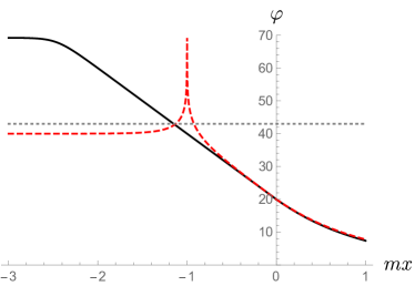
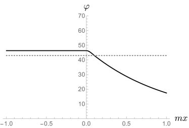
Figure 10: Left: Profiles of the Hartle–Hawking sphaleron (black solid) and a slice of periodic instanton at $\tau=0$ (red dashed) for $\lambda=0.5\Lambda_{HH}$. The center of the periodic instanton is taken at $x_{HH}=-1/m$. The grey dotted line marks the field value $\varphi_{\rm max}$ corresponding to the top of the potential barrier, see Fig. 5. We take $\mathop{\rm ln}\nolimits(m/\sqrt{\kappa})=20$. Right: High-temperature sphaleron for the same model parameters.

For the static sphaleron configuration the general equation (4.4) reduces to

$$\partial_{x}^{2}\varphi_{\rm sph}-m^{2}\,\Omega\,\varphi_{\rm sph}+2\kappa\,\Omega\,{\rm e}^{\varphi_{\rm sph}}=0\;.$$ (5.11)

Its solution can be easily found numerically for any given values of parameters. In the previous subsection we have found the solution analytically at $\lambda<\Lambda_{HH}$. Now we construct it in the opposite limit $\lambda\gg\Lambda_{HH}$.

We notice that at high BH temperatures, $\Omega$ can be approximated by a step-function: $\Omega=0$ at $x<0$ and $\Omega=1$ and $x>0$. Therefore, Eq. (5.11) can be solved separately at negative and positive $x$, with matching at $x=0$. In the inner region, $x<0$, the equation is simply $\partial_{x}^{2}\varphi_{\rm sph}=0$. Requiring regularity at the horizon leads to a constant solution, $\varphi_{\rm sph}(x<0)=$ const. In the outer region, $x>0$, the equation coincides with the flat-space one. Hence, one can employ the same strategy as with the flat-space sphaleron studied in Sec. 3.1: find the nonlinear core centered at $x=0$ (as required for the smooth matching with the inner region) and glue it with the massive linear tail. Overall, we obtain

$$\varphi_{\rm sph}=\begin{cases}\mathop{\rm ln}\nolimits\frac{\Lambda_{0}^{2}}{\kappa}\;,&x<0\\ \mathop{\rm ln}\nolimits\left[\frac{\Lambda_{0}^{2}}{\kappa\mathop{\rm ch}\nolimits^{2}(\Lambda_{0}x)}\right]\;,&x>0\;,~{}~{}x\ll 1/m\\ \frac{2\Lambda_{0}}{m}{\rm e}^{-mx}\;,&x>0\;,~{}~{}x\gg 1/\Lambda_{0}\end{cases}$$ (5.12)

where $\Lambda_{0}$ is given in Eq. (3.9). The solution is shown in the right panel of Fig. 10.

As $\lambda\to\infty$, the physical size of the near-horizon region shrinks to zero. Hence, the high-temperature Hartle–Hawking sphaleron is just a half of the flat-space sphaleron. Correspondingly, its energy is one half of the energy of the flat-space sphaleron (cf. Eqs. (3.10), (3.11)),

$$E_{\text{sph, high-}\lambda}=\frac{1}{{\rm\text{g}}^{2}}\int_{-\infty}^{\infty}dx\,\Omega(x)\kappa(\varphi_{\rm sph}-2){\rm e}^{\varphi_{\rm sph}}\approx\frac{2\Lambda_{0}}{{\rm g}^{2}}\left(\mathop{\rm ln}\nolimits\frac{\Lambda_{0}}{\sqrt{\kappa}}-2+\mathop{\rm ln}\nolimits 2\right)\;.$$ (5.13)

This reduction of the sphaleron energy by a factor 2 can be viewed as the purely geometric effect of the BH on the height of the energy barrier between the false and true vacua. Its analog in four-dimensional Schwarzschild metric was studied in [29, 34]. Finally, the tunneling suppression due to the Hartle–Hawking sphaleron at high temperatures is

$$B_{HH}=\frac{4\pi\Lambda_{0}}{{\text{g}}^{2}\lambda}\left(\mathop{\rm ln}\nolimits\frac{\Lambda_{0}}{\sqrt{\kappa}}-2+\mathop{\rm ln}\nolimits 2\right)~{},~{}~{}~{}~{}~{}\lambda\gg\Lambda_{HH}\;.$$ (5.14)

At $\lambda\simeq\Lambda_{HH}$ this expression matches with (5.7) to the leading-log approximation, providing a smooth transition between the low- and high-temperature regimes.

It is worth mentioning that, similarly to the flat-space case, the tunneling rate at high BH temperature can be estimated using the stochastic picture. From the expressions for the Green’s function at close separation — the upper line in Eq. (B.34) and Eq. (B.36) — one reads out the variance of the thermal fluctuations of the field in the neighborhood of the BH,

$$\delta\varphi_{HH}^{2}\approx\frac{{\rm g}^{2}\lambda}{2\pi m}\;.$$ (5.15)

Note that it is twice bigger than in flat space at the same temperature, Eq. (3.35), due to the contribution of modes localized on the BH. This gives the vacuum decay rate

$$\varGamma_{HH,\,\text{high-}\lambda}\sim\exp\left(-\frac{\varphi_{\rm max}^{2}}{2\delta\varphi_{HH}^{2}}\right)\sim\exp\left[-\frac{4\pi m}{{\rm g}^{2}\lambda}\left(\mathop{\rm ln}\nolimits\frac{m}{\sqrt{\kappa}}\right)^{2}\right]\;.$$ (5.16)

It coincides with the suppression (5.14) in the leading-log approximation.

Figure 11: Suppression of the decay rate of the Hartle–Hawking vacuum as a function of the BH temperature $T_{BH}=\lambda/(2\pi)$ (thick line). Transition between the low- and high-temperature regimes occurs at $\Lambda_{HH}$ given by Eq. (5.6). The tunneling suppression in flat spacetime at the same temperature is shown with the thin line (cf. Fig. 8). For $\Lambda_{0}$ and $B_{M}$ see Eqs. (3.9), (3.21).

Let us summarize. At low temperatures, the decay of the Hartle–Hawking vacuum in the vicinity of a BH proceeds via periodic configurations. One of these configurations is static, and it is plausible that it is actually preferred when the subleading corrections to the metric are taken into account. The suppression is given by Eq. (5.7). At the critical temperature $\Lambda_{HH}$ the nonlinear core of the tunneling solution stops fitting the near-horizon region. At higher temperatures, the tunneling proceeds via the sphaleron that extends outside the near-horizon region, and the tunneling suppression is half of that in flat space. The summary of our findings is shown in Fig. 11.

5.2 Unruh vacuum

5.2.1 Tunneling far from the black hole

The Unruh state corresponds to a flux of thermal radiation emitted by the BH. In one spatial dimension the flux propagates without spreading and leads to an enhancement of vacuum decay rate at an arbitrary distance from the BH. It is instructive to first consider this case, where tunneling proceeds in flat geometry, with the difference from the Minkowski vacuum entirely due to the presence of (out-of-equilibrium) excitations. This will serve us as a benchmark for the subsequent study of tunneling near horizon where both effects of the geometry and excitations are present.

Specifically, we look for a bounce centered at $x_{1}\gg 1/m$. The Euclidean formalism is no longer useful, so we work with the Lorentzian time $t$ and construct the solution on the contour ${\cal C}$ of Sec. 2.4. As before, we assume that outside the nonlinear core, the solution is proportional to the time-ordered Green’s function,

$$\varphi_{\rm b}\Big{|}_{\rm tail}=8\pi\mathcal{G}_{U}(t,x;0,x_{1})\;,$$ (5.17)

where we take the same proportionality coefficient as in the cases studied above. When $(t,x)$ gets close to the center $(0,x_{1})$, the tail must be matched to the solution (3.5) of the nonlinear Liouville equation. The Green’s function at close separation for the case at hand is given by the lower line in Eq. (B.43) from the Appendix. Its singular part is a mixture of a thermal contribution for the right-moving modes and a vacuum contribution for left-movers. This suggests to take the thermal (vacuum) Ansatz for the function $F$ ($G$) of the general Liouville solution. Namely, we write

$$F(-u)=\frac{C_{U1}}{\lambda}\left({\rm e}^{-\lambda(u-u_{1})}-1\right)\;,~{}~{}~{}~{}~{}G(v)=C_{U1}(v-v_{1})\;,$$ (5.18)

where $v_{1}=-u_{1}=x_{1}$ and $C_{U1}$ is an unknown constant. Substituting this into Eq. (3.5), we obtain

$$\varphi_{\rm b}\Big{|}_{\rm core}=\mathop{\rm ln}\nolimits\left[\frac{4\lambda^{2}b_{U1}}{\kappa\left(-2\lambda(v-v_{1})\mathop{\rm sh}\nolimits\left(\frac{\lambda}{2}(u-u_{1})\right)+b_{U1}{\rm e}^{\frac{\lambda}{2}(u-u_{1})}\right)^{2}}\right]$$ (5.19)

with

$$b_{U1}=\frac{\lambda^{2}}{\kappa C_{U1}^{2}}\;.$$ (5.20)

This indeed matches to Eq. (B.43) (lower line) describing the Green’s function at close separation when the first term in the denominator wins over the second,

$$\left|2\lambda(v-v_{1})\mathop{\rm sh}\nolimits\left(\tfrac{\lambda}{2}(u-u_{1})\right)\right|\gg\left|b_{U1}{\rm e}^{\frac{\lambda}{2}(u-u_{1})}\right|\;.$$ (5.21)

Equating the constant parts in $\varphi_{\rm b}\big{|}_{\rm core}$ and $\varphi_{\rm b}\big{|}_{\rm tail}$ fixes

$$b_{U1}=\frac{\kappa}{m^{2}}\>{\rm e}^{\frac{8\lambda}{3\pi m}-2\gamma_{E}+\frac{1}{2}}\;.$$ (5.22)

Note that $b_{U1}\ll 1$ for not-so-large $\lambda\gtrsim m$, but grows exponentially with $\lambda$.

Clearly, the solution (5.17), (5.19) is real on the real time axis and describes run-away towards $\varphi\to+\infty$ at positive time. What distinguishes it from vacuum or thermal bounces, is the absence of a constant-time slice on which the solution would have zero time derivative $\dot{\varphi}_{\rm b}$. The profiles of $\varphi_{\rm b}$ and $\dot{\varphi}_{\rm b}$ at $t=0$ are shown in Fig. 12.

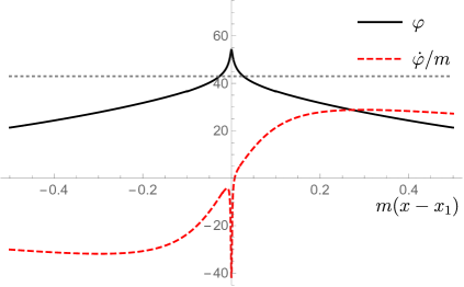
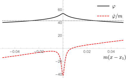
Figure 12: Bounce solution describing tunneling from the Unruh vacuum far away from the BH. Left: Profiles of the bounce (black solid) and its time derivative (red dashed) at $t=0$ for $\lambda=0.87\Lambda_{U1}$, where $\Lambda_{U1}$ is defined in Eq. (5.25). Right: Zoom-in on the central region of the left plot. We take $\mathop{\rm ln}\nolimits(m/\sqrt{\kappa})=20$. The grey dotted line marks the field value $\varphi_{\rm max}$ at the maximum of the potential barrier, see Fig. 5.

Let us scrutinize the matching procedure. For this purpose, we deform the contour ${\cal C}$ on which the bounce is defined into ${\cal C}^{\prime}$ consisting of semi-infinite parts at $\mathop{\rm Im}\nolimits t=\pm\pi/\lambda$, $\mathop{\rm Re}\nolimits t<0$ and a Euclidean portion at $-\pi/\lambda<\mathop{\rm Im}\nolimits t<\pi/\lambda$, $\mathop{\rm Re}\nolimits t=0$ (see Fig. 7a). If

$$b_{U1}\ll 1\;,$$ (5.23)

the core of the bounce fits entirely inside the Euclidean part of the contour. In other words, the matching region where (5.21) is satisfied surrounds the core in Euclidean time. This region also comfortably overlaps with the domain of validity of the expression for the Green’s function at close separation, which is bounded by (see Appendix B.2)

$$|x-x_{1}|,~{}|t|\ll 1/\sqrt{\lambda m}\;.$$ (5.24)

On the other hand, when $b_{U1}>1$, the matching procedure in Euclidean time breaks down. It is unclear if it can be extended to higher values of $b_{U1}$ by matching on the parts of the contour parallel to the real axis. A careful analysis of this issue would require studying corrections to the core and tail of the bounce which is beyond the scope of this paper. Thus, we take (5.23) as a conservative condition for the validity of the bounce solution constructed above. In view of the formula (5.22), it translates into an upper bound on the BH temperature, $\lambda\lesssim\Lambda_{U1}$, where

$$\Lambda_{U1}=\dfrac{3\pi m}{4}\bigg{(}\mathop{\rm ln}\nolimits\frac{m}{\sqrt{\kappa}}+\gamma_{E}-\frac{1}{4}\bigg{)}\;.$$ (5.25)

We will discuss what happens at higher BH temperatures shortly.

Turning to the tunneling suppression, we need to compute the integral (2.53). Unlike Minkowski or thermal cases, we cannot deform the contour to cast this integral into the form of an Euclidean action. Therefore, we work directly with the contour ${\cal C}$. The computation requires some care and is relegated to Appendix D. The result reads

$$B_{U1}=\frac{16\pi}{\text{g}^{2}}\bigg{(}\mathop{\rm ln}\nolimits\sqrt{\frac{\lambda m}{\kappa}}-\frac{2\lambda}{3\pi m}+\frac{\mathop{\rm ln}\nolimits 2+\gamma_{E}}{2}-\frac{9}{8}\bigg{)}\;,~{}~{}~{}~{}~{}\lambda\lesssim\Lambda_{U1}\;.$$ (5.26)

Notice that the leading logarithmic part of the suppression can be easily found by the method outlined at the end of Sec. 3.2 which relates it to the field value at the core of the bounce. Substituting

$$\varphi_{\rm b}(t=0,x=x_{1})\approx\mathop{\rm ln}\nolimits\bigg{(}\frac{4\lambda^{2}}{\kappa b_{U1}}\bigg{)}$$ (5.27)

into Eq. (3.22) and using Eq. (5.22), we indeed recover Eq. (5.26) up to order-one corrections in the brackets.

We observe that the suppression decreases with the BH temperature and reaches down to approximately half of the vacuum suppression at $\lambda\approx\Lambda_{U1}$. Comparing it with the suppression of the flat thermal bounce (3.30), we see that the main difference is in the linear-in-$\lambda/m$ term. The latter is smaller in the case of Unruh vacuum, hence tunneling from it is more suppressed. This is, of course, expected due to the deviation of the Unruh state from thermality.

We presently discuss transitions at BH temperature higher than $\Lambda_{U1}$. The lessons learned from thermal and Hartle–Hawking cases suggest that this will be driven by jumps onto sphaleron. An indication in favour of this guess is that the value of the field in the core of the bounce (5.19) decreases from $\sim 4\mathop{\rm ln}\nolimits(m/\sqrt{\kappa})$ at $\lambda\approx m$ (the value in the center of the Minkowski bounce) down to $\sim 2\mathop{\rm ln}\nolimits(m/\sqrt{\kappa})\approx\varphi_{\rm max}$ at $\lambda\approx\Lambda_{U1}$, which is the same as the value in the center of the sphaleron. Of course, due to asymmetry of the Unruh particle flux, the sphaleron will not be produced at rest. Rather, one expects the created sphaleron to move in the direction of the flux and be accompanied by particle excitations (see [56, 45, 63, 64, 55] for the formation of similar “excited sphalerons” in quantum mechanical and field theoretical models). Our analytic cut-and-match procedure does not allow us to capture this type of solutions, which do not have a well-localized core in time and space.

Still, we can try to estimate the corresponding suppression using the stochastic approach, which we saw to give the right leading-log results for the thermal and Hartle–Hawking vacuum decays. We expect it to work in the Unruh case as well, because the Unruh flux in our model is dominated by soft modes with low frequencies $\omega\sim m\ll\lambda$ and large occupation numbers. In other words, the fluctuations of the field in this flux are essentially semiclassical. This will lead to classical “jumps on the barrier”, for which the stochastic picture provides a fair description.

Similarly to Eq. (3.35), we estimate the field fluctuations in the Unruh flux as

$$\delta\varphi_{U1}^{2}=\text{g}^{2}\lim_{\begin{smallmatrix}t\to 0\\ x\to x_{1}\end{smallmatrix}}\big{[}\mathcal{G}_{U}(t,x;0,x_{1})-\mathcal{G}_{F}(t,x;0,x_{1})\big{]}\approx\frac{{\rm g}^{2}\lambda}{3\pi^{2}m}\;,$$ (5.28)

where we have used the lower line of Eq. (B.43) and retained only the leading term. Then, the vacuum decay rate is

$$\varGamma_{U1,\,\text{high-}\lambda}\sim\exp\left(-\frac{\varphi_{\rm max}^{2}}{2\delta\varphi_{U1}^{2}}\right)\sim\exp\left[-\frac{6\pi^{2}m}{{\rm g}^{2}\lambda}\left(\mathop{\rm ln}\nolimits\frac{m}{\sqrt{\kappa}}\right)^{2}\right]\;.$$ (5.29)

At $\lambda\approx\Lambda_{U1}$ the stochastic estimate coincides with the bounce suppression (5.26) in the leading-log approximation. It is exponentially smaller than the thermal rate (3.36). Still, it reaches order-one values at $\lambda\to\infty$. In other words, the exponential suppression disappears at high enough BH temperatures. As we will explain in Sec. 6, we believe this property to be special for our model and do not expect it to be generic.

The results of this subsection for the suppression of the Unruh vacuum decay far from the BH are summarized in Fig. 13.

Figure 13: Suppression of the Unruh vacuum decay far from the BH as a function of the BH temperature $T_{BH}=\lambda/(2\pi)$ (thick line). The transition between the low-temperature bounces and the high-temperature stochastic jumps happens at $\Lambda_{U1}$, see Eq. (5.25). Thin line shows for comparison the suppression of false vacuum decay in a thermal bath with the same temperature. Expressions for $\Lambda_{0}$ and $B_{M}$ are given in Eqs. (3.9), (3.21).

5.2.2 Tunneling near horizon

In the BH vicinity the vacuum decay is affected both by excitations and by the nontrivial geometry. The latter significantly contributes to the enhancement of the decay rate, as we are now going to see.

With the insight from the previous subsection, we can immediately write down the Ansatz for the bounce centered at a point $(t_{2},x_{2})$ in the near-horizon region,

$$\varphi_{\rm b}\Big{|}_{\rm core}=\mathop{\rm ln}\nolimits\left[\frac{4\lambda^{2}b_{U2}}{\kappa\left(-2\lambda(v-v_{2})\mathop{\rm sh}\nolimits\left(\frac{\lambda}{2}(u-u_{2})\right)+b_{U2}\,{\rm e}^{\frac{\lambda}{2}(u-u_{2})}\right)^{2}}\right]-2\lambda x\;,$$ (5.30a)

$$\varphi_{\rm b}\Big{|}_{\rm tail}=8\pi\mathcal{G}_{U}(t,x;t_{2},x_{2})\;,$$ (5.30b)

where $u_{2}=t_{2}-x_{2}$, $v_{2}=t_{2}+x_{2}$. The term $-2\lambda x$ in the first expression comes from the metric factor $\Omega(x)$ in the general solution (4.5) of the Liouville equation in the near-horizon geometry. The Green’s function at close separation near horizon is given by Eq. (B.47) from Appendix B. Matching it to the asymptotics of the expression (5.30a), we find

$$b_{U2}=\bar{b}_{U2}{\rm e}^{-2\lambda x_{2}}~{},~{}~{}~{}~{}~{}\bar{b}_{U2}=\frac{\kappa}{m^{2}}{\rm e}^{\frac{32\lambda}{3\pi m}-2\gamma_{E}-\frac{3}{2}}\;.$$ (5.31)

Let us discuss the conditions for the validity of the matching procedure, which are quite subtle. It is convenient to introduce the advance Kruskal coordinate $\bar{u}$ as in Eq. (2.11). In the new coordinates $(\bar{u},v)$ the expression for the bounce core takes the form

$$\varphi_{\rm b}\Big{|}_{\rm core}=\mathop{\rm ln}\nolimits\left[\frac{4\lambda^{2}\bar{b}_{U2}{\rm e}^{-\lambda v_{2}}}{\kappa\left(-\lambda^{2}(v-v_{2})(\bar{u}-\bar{u}_{2})+\bar{b}_{U2}{\rm e}^{-\lambda v_{2}}\right)^{2}}\right]-\lambda v\;,$$ (5.32)

where $\bar{u}_{2}=-\lambda^{-1}{\rm e}^{-\lambda u_{2}}$. We observe that, apart from the last linear-in-$v$ term, this has the same form as for the bounce in flat spacetime. The expression (B.47) for the Green’s function at close separation is valid as long as all points are in the near-horizon region and $|v-v_{2}|\ll 1/\sqrt{\lambda m}$ (note that there are no restrictions on $|u-u_{2}|$). Thus, the matching region in the two-dimensional complex space of variables $(\bar{u},v)$ is determined by the conditions

$$\big{|}\lambda^{2}(v-v_{2})(\bar{u}-\bar{u}_{2})\big{|}\gg\bar{b}_{U2}{\rm e}^{-\lambda v_{2}}~{},~{}~{}~{}~{}~{}|v-v_{2}|\ll 1/\sqrt{\lambda m}~{},~{}~{}~{}~{}~{}\mathop{\rm Re}\nolimits\big{(}\lambda v+\mathop{\rm ln}\nolimits(-\lambda\bar{u})\big{)}<0\;.$$ (5.33)

The last condition here ensures that in the matching region one can use the near-horizon form of the metric. We additionally require that there must be a continuous deformation of the contour ${\cal C}$, such that on this deformation the matching region surrounds the core.

The combination of the first and last conditions in (5.33) turns out to provide the strongest restrictions. Any deformation of the contour must cross the wedge where both $\bar{u}$ and $v$ are real and $\bar{u}<\bar{u}_{2}$, $v>v_{2}$ (i.e., the right wedge with respect to the point $(u_{2},v_{2})$ in the original coordinates). The possibility to have an overlap on this intersection implies that there is $v_{*}>v_{2}$, such that

$$\lambda(v_{*}-v_{2})\big{(}{\rm e}^{-\lambda(v_{*}-v_{2})}+\lambda\bar{u}_{2}{\rm e}^{\lambda v_{2}}\big{)}\gg\bar{b}_{U2}.$$ (5.34)

Given that $\bar{u}_{2}<0$, the l.h.s. of the above inequality does not exceed a value of order one. Hence, we conclude that the necessary condition for matching is

$$\bar{b}_{U2}\ll 1\;.$$ (5.35)

One can verify that this condition is also sufficient. It restricts the validity of the bounce solutions (5.30) to $\lambda\lesssim\Lambda_{U2}$, where

$$\Lambda_{U2}=\frac{3\pi m}{16}\bigg{(}\mathop{\rm ln}\nolimits\frac{m}{\sqrt{\kappa}}+\gamma_{E}+\frac{3}{4}\bigg{)}\;.$$ (5.36)

Note that this critical temperature is higher than its counterpart (5.6) for tunneling from the Hartle–Hawking vacuum.

Similarly to the Hartle–Hawking case, we have obtained a family of bounces parameterized by the position of the center. Their shape depends on $x_{2}$. Still, their suppression is $x_{2}$-independent and reads (see Appendix D for the calculation)

$$B_{U2}=\frac{16\pi}{\text{g}^{2}}\left(\mathop{\rm ln}\nolimits\sqrt{\frac{\lambda m}{\kappa}}-\dfrac{8\lambda}{3\pi m}+\frac{\mathop{\rm ln}\nolimits 2+\gamma_{E}}{2}-\frac{5}{8}\right)\;,~{}~{}~{}~{}~{}\lambda\lesssim\Lambda_{U2}\;.$$ (5.37)

This implies less suppression than for tunneling far away from the BH, Eq. (5.26). The enhancement of the transition rate is due to the excitation of modes localized on the BH by the potential barrier $U_{\rm eff}(x)=m^{2}\Omega(x)$ (see Fig. 3). The existence of such localized states is, in turn, a consequence of the nontrivial geometry. On the other hand, as one could conjecture [3], the suppression is stronger than for the decay of the Hartle–Hawking vacuum, Eq. (5.7). Our result (5.37) provides the first confirmation of this conjecture from first principles.

As in the Hartle–Hawking case, we expect the degeneracy between the bounces with different $x_{2}$ to be lifted if we take into account deviation of the near-horizon metric from the Rindler form. What is then the least suppressed solution? A natural candidate is the “Unruh sphaleron” obtained by taking the limit $\bar{u}_{2}\to 0^{-}$ in Eq. (5.32). Setting for simplicity $v_{2}=0$, we have in the original coordinates

$$\varphi_{\rm sph}\Big{|}_{\rm core}=\mathop{\rm ln}\nolimits\left[\frac{4\lambda^{2}\bar{b}_{U2}}{\kappa(\lambda v\,{\rm e}^{-\lambda u}+\bar{b}_{U2})^{2}}\right]-\lambda v\;.$$ (5.38)

This solution is regular at $t>0$, thus it does not exhibit run-away towards the true vacuum. We conjecture that it may instead describe at late times formation of the Hartle–Hawking sphaleron of Sec. 5.1 plus excitations flying away from the BH. Our analytic method does not allow us to trace this late-time evolution, which would require a numerical study. Notice that, unlike any other solutions considered so far, the sphaleron profile (5.38) diverges linearly when $x\to-\infty$ at fixed $t$. We do not know if this is a serious drawback. The above limit corresponds to approaching the bifurcation point between the past and future horizons on the extended Penrose diagram of the BH spacetime, see Fig. 2. So, the divergence is consistent with the fact that the Unruh vacuum is singular on the past horizon. On the other hand, it violates an implicit assumption made throughout our analysis that the field is bounded at $x\to-\infty$. In any case, even if the sphaleron (5.38) should be excluded from the space of admissible solutions, it is likely to reappear as the limiting configuration of regular bounces (5.30) that in the full treatment will arise as constrained instantons (cf. [79]).

Figure 14: Suppression of the Unruh vacuum decay as a function of BH temperature $T_{BH}=\lambda/(2\pi)$ (thick line). The critical temperature $\Lambda_{U2}$ (Eq. (5.36)) marks the transition from the low-temperature regime dominated by bounce solutions in the near-horizon region to high-temperature stochastic jumps over the potential barrier. The suppression of the Hartle–Hawking vacuum decay is shown by the thin line for comparison, with the critical temperature $\Lambda_{HH}$ given by Eq. (5.6). $B_{M}$ is the value of the suppression in the absence of BH, Eq. (3.21).

At BH temperature above $\Lambda_{U2}$, the bounce core stops fitting into the near-horizon region, and our analytic method fails to produce the solution. However, we can again estimate the tunneling rate using the stochastic picture. From the expression (B.43) (upper line) for the Green’s function outside, but not very far from the BH we read out the amplitude of the field fluctuations,

$$\delta\varphi_{U2}^{2}\approx\frac{4{\rm g}^{2}\lambda}{3\pi^{2}m}\;.$$ (5.39)

Substituting this into the estimate of the decay rate gives

$$\varGamma_{U2,\,\text{high-}\lambda}\sim\exp\left(-\frac{\varphi_{\rm max}^{2}}{2\delta\varphi_{U2}^{2}}\right)\sim\exp\left[-\frac{3\pi^{2}m}{2{\rm g}^{2}\lambda}\left(\mathop{\rm ln}\nolimits\frac{m}{\sqrt{\kappa}}\right)^{2}\right]\;.$$ (5.40)

We observe that in the leading-log approximation the suppression is continuous across the transition from the low- to high-temperature regime.

The suppression of the false vacuum decay from the Unruh vacuum is plotted in Fig. 14, where it is compared to the suppression of tunneling from the Hartle–Hawking state. We see that the former is always larger than the latter, though it also goes to zero with the increase of the BH temperature. The situation is qualitatively similar to the case of tunneling far away from the BH, cf. Fig. 13. We are going to argue, however, that vanishing of the Unruh suppression at high BH temperature is not expected to be generic.

6 Discussion and outlook

In this paper we have developed an approach for the analysis of false vacuum decay in BH background. This approach is rooted in the in-in formalism and treats various vacua in the BH geometry as mixed states. It reduces the task of finding the vacuum decay rate to the solution of classical field equations on a contour in complex Schwarzschild time. The solution — bounce — must interpolate between the basins of attraction of the false and true vacua and is subject to boundary conditions in the asymptotic past that encode the details of the initial quantum state. These are the same boundary conditions as for the time-ordered Green’s function in the respective state. They allow one to discriminate between different vacua in the BH background: Boulware, Hartle–Hawking and Unruh.

Our method is general and can be applied to many situations other than an isolated BH. For example, realistic BHs in the early Universe are immersed in thermal plasma whose temperature may be different from that of the BH [34]. Another example of nontrivial environment is the de Sitter spacetime relevant for inflation, which also possesses its own ambient temperature. These cases present an interesting arena for the use of our approach. Our method can also be of interest beyond the BH physics, for the study of tunneling in various non-equilibrium quantum systems.

It is worth comparing our method to the approach of [80, 81] proposing to describe tunneling as classical evolution with stochastic initial conditions. Despite some resemblance, there are important differences. Refs. [80, 81] assume that the fields are purely real and evolve in real time. Whereas in our method the tunneling solutions are essentially complex and live on a contour in the complex time that in general cannot be continuously deformed into the real axis because of branch-cut singularities. Further, in the case of false vacuum decay in flat space the stochastic approach tends to significantly overestimate the decay rate [82], whereas our method recovers exactly the results of the standard Euclidean description. On the other hand, we expect the stochastic approach to work well for tunneling from states with large occupation numbers [75, 76, 77, 78], such as the Hartle–Hawking and Unruh vacua in the background of a two-dimensional BH with high temperature. It will be interesting to apply the method of [80, 81, 82] to this case and compare it with our results.

We have demonstrated the efficiency of our method on an example of a two-dimensional scalar toy model with self-interaction given by the inverted Liouville potential. Due to the specific properties of the model, the bounce solutions could be found analytically in most regimes. Their structure is in a sense opposite to the widely used thin-wall picture where the size of the bounce solution is much larger than the Compton wavelength of the field. By contrast, the bounces in our model have a tiny nonlinear core with the size much smaller than the Compton wavelength, and a wide tail of size $1/m$ where the field is linear.

Using this example, we connected our method to the standard Euclidean approach to tunneling from equilibrium states, such as the flat-space vacuum, thermal bath and the Hartle–Hawking state. We clarified several details of these processes along the way. We further found the bounce solutions describing decay of the Unruh vacuum where the Euclidean formalism is not available.

In the Hartle–Hawking case the tunneling regime changes from what can be called “direct tunneling” at low BH temperature, where the bounce describes run-away to the true vacuum at late times, to the “sphaleron-driven” transitions at high temperature that proceed via formation of the sphaleron. The latter can be viewed as jumps on the saddle point of the potential separating the two vacua, driven by stochastic thermal fluctuations. We saw indications of a similar change of the tunneling regime in the case of Unruh vacuum, but were unable to find the high-temperature sphaleron-forming solutions analytically. Still, we could estimate the tunneling suppression using the stochastic picture and showed that it continuously connects in the leading order to the rate found from the analytic bounces at low temperature. It will be interesting to perform a numerical study of the high-temperature Unruh bounces in order to rigorously establish the transition between different tunneling regimes and refine the computation of the transition rate at high BH temperatures.

To our knowledge, the present work gives the first calculation of the catalyzing effect of BH on vacuum decay fully taking into account the structure of the Unruh state. This catalyzing effect is twofold. Part of it is due to the change in geometry. Another part is due to the excitation of the field modes by the BH. We found that the two effects are of the same order and are closely intertwined. Namely, the gravitational redshift near the BH horizon gives rise to extra states localized on the BH, in addition to the modes radiated away to infinity. These bound states get excited and significantly enhance the field fluctuations in the BH vicinity, thereby facilitating the vacuum decay.

Our results confirm the conjecture [3] that the decay rate of the Unruh vacuum is exponentially smaller than that of the Hartle–Hawking state. Still, we found that the suppression disappears at high BH temperature. As discussed in the Introduction, if this result were to hold for realistic four-dimensional BHs, it would have dramatic consequences for phenomenological model building. There are, however, important properties of the four-dimensional setup that are not captured by the two-dimensional model and may alter the conclusion.

One of them is the structure of the effective potential for the field modes. In the two-dimensional case, it is a monotonic function of the tortoise coordinate $x$, varying between $0$ and $m^{2}$, see Fig. 3. This allows all modes with frequencies below and of order $m$ to contribute into the field fluctuations within the distance $\sim 1/m$ from the horizon. Due to large occupation numbers, these modes dominate tunneling at high temperature. On the other hand, the effective potential in the Schwarzschild metric, obtained upon spherical reduction, has the form depicted in Fig. 15. The important new feature is the presence of a potential barrier with the height scaling as $\sim r_{h}^{-2}$, where $r_{h}$ is the Schwarzschild radius. It suppresses the escape of the low-frequency modes, the effect being encapsulated by the well-known fall-off of the BH grey-body factors at small $\omega$. This is expected to suppress the field fluctuations outside the BH resulting in a qualitatively different behavior of the vacuum decay rate at high temperature [30]. Another effect that is expected to further reduce particle number density outside the BH is the geometric $1/r^{2}$ spreading of the particle flux. The general formalism developed in Sec. 2 of the paper in principle allows one to take both these effects into account, and we plan to return to this topic in future work.

Figure 15: Effective potential for spherically symmetric linear massive modes in the four-dimensional Schwarzschild geometry.

One more direction for future research is calculation of the pre-exponential factor in the decay rate formula (2.51). Of course, its effect is subleading to that of the exponential suppression which was the focus of this paper. Still, it is important to set the overall dimensionful scale of the rate. A related question is inclusion of the thermal corrections to the scalar field potential. Again, these are generally expected to be small [33], but may be enhanced in theories with large number of particle species and not-so-small couplings [34, 32]. The latter class includes the Standard Model — admittedly, the most interesting case from the phenomenological perspective.

Finally, one would like to include dynamical gravity. This would open the way to address such questions as the relation between the tunneling probability and the BH entropy, or the possibility for a complete BH disappearance as a result of tunneling [13]. Several obstacles must be overcome to achieve this goal. The most important one is the generalization of the boundary conditions on the bounce solution formulated in this work to the case when the position of the BH horizon is not fixed, but is itself a dynamical variable.

Appendix A Dilaton black holes

Two-dimensional dilaton gravity includes the metric $g_{\mu\nu}$ and the dilaton $\phi$ with the action [83]

$$S_{\rm DG}=\int d^{2}x\sqrt{-g}\;{\rm e}^{-2\phi}\big{[}R+4(\nabla_{\mu}\phi)^{2}+4\lambda^{2}\big{]}\;.$$ (A.1)

Here $R$ is the scalar curvature and $\lambda$ is a constant parameter. The strength of gravitational interactions is governed by the field-dependent coupling ${\rm e}^{2\phi}$. The theory admits a one-parameter family of solutions with the metric of the form (2.2) and

$$\Omega=1-\frac{M}{2\lambda}{\rm e}^{-2\lambda r}~{},~{}~{}~{}~{}~{}\phi=-\lambda r\;.$$ (A.2)

They describe BHs with the mass $M$ and horizon radius

$$r_{h}=\frac{1}{2\lambda}\mathop{\rm ln}\nolimits\frac{M}{2\lambda}\;.$$ (A.3)

Introducing the tortoise coordinate

$$x=\frac{1}{2\lambda}\mathop{\rm ln}\nolimits\bigg{(}{\rm e}^{2\lambda r}-\frac{M}{2\lambda}\bigg{)}-\frac{1}{2\lambda}\mathop{\rm ln}\nolimits\frac{M}{2\lambda}$$ (A.4)

and re-expressing $\Omega$ as a function of $x$, we obtain Eq. (2.7) from the main text.

Throughout the paper we neglect the back-reaction of the tunneling field $\varphi$ on the geometry. This is justified if the gravitational coupling is sufficiently small. The maximal value of the coupling in the BH exterior, which is the only region relevant for the false vacuum decay, is achieved at the BH horizon and equals $2\lambda/M$. Thus, the back-reaction can indeed be neglected for heavy enough BHs. Note that due to peculiarities of the two-dimensional theory, the BH temperature does not depend on its mass, being set by the parameter $\lambda$ in the dilaton gravity action.

Appendix B More on modes and Green’s functions

B.1 Solutions to the Shrödinger equation

Here we study some general properties of the massive linear modes $f_{R,\omega}$, $f_{L,\omega}$ introduced in Sec. 2.2 and give their explicit expressions for a number of cases.

B.1.1 General properties

We assume that the effective potential for the modes $U_{\rm eff}(x)$ behaves as $\propto{\rm e}^{2\lambda x}$ at large negative $x$ and goes to $1$ at large positive $x$, see Fig. 3. This is the case for the dilaton BH where $U_{\rm eff}(x)=m^{2}\Omega(x)$ and $\Omega(x)$ is given in Eq. (2.7). In this case the potential grows monotonically as $x$ increases. However, the latter property is not used in this subsection which also applies to more general nonmonotonic potentials like the one in Fig. 15.

The asymptotic expansions of the modes $f_{R,\omega}$, $f_{L,\omega}$ are given in Eqs. (2.16), (2.18). We focus on $\omega>m$ as only in this case two linearly-independent solutions exist and the relation between their expansions is nontrivial. Note that $\gamma_{\omega}$ and $\beta_{\omega}$ are the transmission and reflection amplitudes of the potential $U_{\rm eff}$. We will now show that all other coefficients in the asymptotic expansions (2.16), (2.18) are expressed through these amplitudes.

The eigenfunctions $f_{R,\omega}$, $f_{L,\omega}$ belong to the continuous spectrum of a Schrödinger equation. Thus their norms and orthogonality are determined by their behavior at infinity. Each plane-wave integral should be treated as contributing half of the $\delta$-function,

$$\int_{-\infty}dx\,{\rm e}^{i(\omega-\omega^{\prime})x}\sim\frac{1}{2}\delta(\omega-\omega^{\prime})~{},~{}~{}~{}~{}~{}\int^{+\infty}dx\,{\rm e}^{i(k-k^{\prime})x}\sim\frac{1}{2}\delta(k-k^{\prime})=\frac{k}{2\omega}\delta(\omega-\omega^{\prime})\;.$$

Then the orthogonality and normalization conditions (2.19), (2.20) imply

$$\beta\tilde{\beta}^{*}+\frac{k}{\omega}\gamma\tilde{\gamma}^{*}=0\;,$$ (B.1a)

$$\frac{1}{2}|\alpha|^{2}+\frac{1}{2}|\beta|^{2}+\frac{k}{2\omega}|\gamma|^{2}=1\;,$$ (B.1b)

$$\frac{1}{2}|\tilde{\beta}|^{2}+\dfrac{k}{2\omega}|\tilde{\gamma}|^{2}+\frac{k}{2\omega}|\tilde{\delta}|^{2}=1\;,$$ (B.1c)

where we have omitted the subscript “$\omega$” to avoid clutter of notations. Next, from the viewpoint of the effective Schrödinger equation, the modes $f_{R,\omega}$, $f_{L,\omega}$ represent wavefunctions of a particle scattering off the potential barrier. These wavefunctions preserve the probability flux which gives us two more conditions,

$$|\alpha|^{2}=|\beta|^{2}+\dfrac{k}{\omega}|\gamma|^{2}\;,$$ (B.2a)

$$\dfrac{k}{\omega}|\tilde{\delta}|^{2}=|\tilde{\beta}|^{2}+\dfrac{k}{\omega}|\tilde{\gamma}|^{2}\;.$$ (B.2b)

Finally, we note that the complex conjugated functions $f_{R,\omega}^{*}$, $f_{L,\omega}^{*}$ must be linear combinations of $f_{R,\omega}$, $f_{L,\omega}$ as the latter form a complete set of linearly-independent solutions,

$$f^{*}_{R,\omega}=Af_{R,\omega}+Bf_{L,\omega}\;,~{}~{}~{}~{}f^{*}_{L,\omega}=Cf_{R,\omega}+Df_{L,\omega}\;.$$ (B.3a)

We write these relations at $$x\to\pm\infty A,..,D$$ using the expressions (2.16), (2.18) and equate terms with the same exponential factors to obtain eight conditions on six amplitudes and four complex coefficients . Solving them with respect to the latter gives

$$A=\dfrac{\beta^{*}}{\alpha}\;,~{}~{}~{}B=\dfrac{\gamma^{*}}{\tilde{\delta}}\;,~{}~{}~{}C=\dfrac{\tilde{\beta}^{*}}{\alpha}\;,~{}~{}~{}D=\dfrac{\tilde{\gamma}^{*}}{\tilde{\delta}}\;.$$ (B.3b)

The remaining conditions become

$$\alpha^{*}=\dfrac{|\beta|^{2}}{\alpha}+\dfrac{\gamma^{*}\tilde{\beta}}{\tilde{\delta}}\;, \tilde{\delta}^{*}=\dfrac{\tilde{\beta}^{*}\gamma}{\alpha}+\dfrac{|\tilde{\gamma}|^{2}}{\tilde{\delta}}\;,$$ (B.4a)

$$\dfrac{\tilde{\beta}^{*}\beta}{\alpha}+\dfrac{\tilde{\gamma}^{*}\tilde{\beta}}{\tilde{\delta}}=0\;, \dfrac{\beta^{*}\gamma}{\alpha}+\dfrac{\gamma^{*}\tilde{\gamma}}{\tilde{\delta}}=0\;.$$ (B.4b)

Note that not all of the relations (B.1), (B.2), (B.4) are independent.

From Eqs. (B.1b), (B.2a) we get $|\alpha|=1$ and the relation between the absolute values of $\beta$ and $\gamma$

$$|\gamma_{\omega}|^{2}=\frac{\omega}{k}\big{(}1-|\beta_{\omega}|^{2}\big{)}~{},\qquad\qquad\omega>m\;,$$ (B.5a)

where we have restored the index $$\omega \omega>m$$ and have explicitly emphasized that this relation is valid at . We use the freedom in choosing the overall phase to set

$$\alpha_{\omega}=1\;.$$ (B.5b)

Next, combining Eqs. (B.1c), (B.2b) gives $$|\tilde{\delta}_{\omega}|=\sqrt{\omega/k} \tilde{\delta}_{\omega} \tilde{\gamma}_{\omega} \tilde{\beta}_{\omega}$$. Again, we fix the phase so that is positive real. Finally, the last of Eqs. (B.4b) and Eq. (B.1a) yield the expressions for and . Collecting them together, we get

$$\tilde{\beta}_{\omega}=\sqrt{\frac{k}{\omega}}\,\gamma_{\omega}~{},~{}~{}~{}~{}\tilde{\gamma}_{\omega}=-\sqrt{\frac{\omega}{k}}\,\frac{\gamma_{\omega}\beta^{*}_{\omega}}{\gamma^{*}_{\omega}}~{},~{}~{}~{}~{}\tilde{\delta}_{\omega}=\sqrt{\frac{\omega}{k}}~{},\qquad\qquad\omega>m\;.$$ (B.5c)

Thus, we have expressed all coefficients in terms of the reflection and transmission amplitudes $\beta_{\omega}$, $\gamma_{\omega}$ of the potential $U_{\rm eff}$. It is straightforward to check that the remaining relations in (B.4) are satisfied and do not yield any further restrictions.

B.1.2 Special cases

Dilaton black hole background.

In this case $\Omega$ is given by Eq. (2.7) and the eigenmode equation can be solved exactly,

$$f_{R,\omega}=\mathcal{N}_{\omega}{\rm e}^{ikx}\>_{2}F_{1}\left({\frac{i}{2\lambda}(\omega-k)\>,\>-\frac{i}{2\lambda}(\omega+k)\>,\>-\frac{ik}{\lambda}+1\>;\>-{\rm e}^{-2\lambda x}}\right)\;,$$ (B.6a)

$$f_{L,\omega}=\mathcal{N}_{\omega}\sqrt{\frac{k}{\omega}}{\rm e}^{-i\omega x}\>_{2}F_{1}\left({\frac{i}{2\lambda}(k-\omega)\>,\>-\frac{i}{2\lambda}(\omega+k)\>,\>-\frac{i\omega}{\lambda}+1\>;\>{\rm e}^{2\lambda x}}\right)\theta(\omega-m)\;,$$ (B.6b)

where ${}_{2}F_{1}$ is the hypergeometric function. The momentum $k$ is given by $\sqrt{\omega^{2}-m^{2}}$ when $\omega>m$ and by the analytic continuation $k=i\sqrt{m^{2}-\omega^{2}}$ when $\omega<m$. Only modes $f_{R,\omega}$ exist for $\omega<m$, whereas $f_{L,\omega}$ vanish, which is ensured by the $\theta$-function in Eq. (B.6b). The normalization factor $\mathcal{N}_{\omega}$ reads

$$\mathcal{N}_{\omega}=\frac{\Gamma\left(-\frac{i}{2\lambda}(\omega+k)\right)\Gamma\left(1-\frac{i}{2\lambda}(\omega+k)\right)}{\Gamma\left(-\frac{i\omega}{\lambda}\right)\Gamma\left(1-\frac{ik}{\lambda}\right)}\;.$$ (B.7)

To calculate the Green’s functions, we need the explicit form of the amplitudes $\beta_{\omega}$, $\gamma_{\omega}$ at $\omega\ll\lambda$. Expanding Eqs. (B.6) in the limits $x\to\pm\infty$ and comparing with Eqs. (2.16), (2.18), we obtain

$$\beta_{\omega}=\frac{\omega-k}{\omega+k}~{},~{}~{}~{}~{}\gamma_{\omega}=\frac{2\omega}{\omega+k}\;,~{}~{}~{}~{}~{}~{}~{}~{}\omega\ll\lambda\;.$$ (B.8)

In this derivation we have used the asymptotics of the hypergeometric function following from Eq. (H.2). Note that these amplitudes are the same as for a step-like potential of height $m^{2}$. They are valid both for $\omega>m$ and for $\omega<m$ with the analytic continuation of momentum (2.21).

Rindler metric.

In Sec. 4 we consider dynamics of the scalar field in Rindler spacetime. In this case the eigenmodes are still solutions to the Schrödinger equation (2.15), but now with the effective potential $U_{\rm eff}=m^{2}{\rm e}^{2\lambda x}$ that grows to infinity at large positive $x$. Therefore, there is no separation into left- and right-moving modes: all modes must decay at $x\to+\infty$. The complete set of eigenfunctions is given by

$$f_{\omega}=\sqrt{\frac{4\omega}{\pi\lambda}\mathop{\rm sh}\nolimits\frac{\pi\omega}{\lambda}}\,K_{\frac{i\omega}{\lambda}}\left(\frac{m}{\lambda}{\rm e}^{\lambda x}\right)\;,$$ (B.9)

where $K$ is the modified Bessel function of the second kind. Note that these modes are real. They decay faster than exponentially at $x\to+\infty$ and become a sum of massless plane waves at $x\to-\infty$.

B.2 Green’s functions at close separation

In the main text we use the expressions for various Green’s functions in the dilaton BH background when the two points in their arguments are close to each other. In this Appendix we derive these expressions. Given that the Green’s functions are time-translation invariant, we can set $t^{\prime}=0$. Then we consider the limit

$$|x-x^{\prime}|\ll m^{-1}\;,~{}~{}~{}~{}~{}|t|\ll m^{-1}\;,~{}~{}t^{\prime}=0\;,$$ (B.10)

which we will denote with the superscript “close”. On top of this, to derive analytic formulae, we will assume high BH temperature, $\lambda\gg m$, and will place the two points in the Green’s function either to the right of the transition region where the BH potential changes significantly,

$$x,x^{\prime}>0\;,~{}~{}~{}~{}~{}x,x^{\prime}\gg\lambda^{-1}\qquad\qquad\text{(``right'')},$$ (B.11)

or to the left of it in the near-horizon region,

$$x,x^{\prime}<0\;,~{}~{}~{}~{}~{}|x|,|x^{\prime}|\gg\lambda^{-1}\qquad\qquad\text{(``left'')}.$$ (B.12)

In these regions we can use the asymptotics for the mode functions in terms of plane waves (2.16), (2.18). Note that in both cases $|x+x^{\prime}|$, can be smaller or larger than $m^{-1}$.

B.2.1 Boulware Green’s function

Right region $x,x^{\prime}>0$.

Using the expression (2.32) and the asymptotics of the mode functions (2.16), (2.18) with the relations between the coefficients (B.5), we obtain

$$\begin{split}&\mathcal{G}_{B}\big{|}_{\rm right}=\int_{m}^{\infty}\frac{d\omega}{4\pi k}\big{[}{\rm e}^{ik(x-x^{\prime})}+{\rm e}^{-ik(x-x^{\prime})}\big{]}{\rm e}^{-i\omega|t|}\\ &-\int_{m}^{\infty}\frac{d\omega}{4\pi k}\bigg{[}\frac{\gamma_{\omega}\beta_{\omega}^{*}}{\gamma_{\omega}^{*}}{\rm e}^{ik(x+x^{\prime})}+\frac{\gamma_{\omega}^{*}\beta_{\omega}}{\gamma_{\omega}}{\rm e}^{-ik(x+x^{\prime})}\bigg{]}{\rm e}^{-i\omega|t|}+\int_{0}^{m}\frac{d\omega}{4\pi\omega}|\gamma_{\omega}|^{2}{\rm e}^{-\varkappa(x+x^{\prime})-i\omega|t|},\end{split}$$ (B.13)

where $k$ and $\varkappa$ are defined in Eqs. (2.17) and (2.21). In the first line we recognize the expression for the Feynman Green’s function in flat spacetime given by Eq. (3.20). At close separation it reduces to

$$\mathcal{G}_{F}\big{|}^{\rm close}=-\frac{1}{4\pi}\mathop{\rm ln}\nolimits\big{[}m^{2}(x-x^{\prime}-t)(x-x^{\prime}+t)+i\epsilon\big{]}+\frac{\mathop{\rm ln}\nolimits 2-\gamma_{E}}{2\pi}\;,$$ (B.14)

where $\gamma_{E}$ is the Euler constant. Notice that away from the coincident points it splits into a sum of right- and left-moving contributions depending only on $(x-x^{\prime}-t)$ and $(x-x^{\prime}+t)$, respectively.

The terms in the second line of Eq. (B.13), which we denote by $\mathcal{G}_{B}^{(2)}\big{|}_{\rm right}$, arise due to the nontrivial BH potential. To compute them, we make the following transformations. First, we use the expressions (B.8) for the reflection and transmission amplitudes. Second, we notice that the integrals in $\mathcal{G}_{B}^{(2)}\big{|}_{\rm right}$ are saturated by $\omega\sim m$, implying that we can use $\omega|t|\ll 1$ to drop the time dependence in the integrands. Third, we change the integration variable from $\omega$ to $k$ in the first integral and to $\varkappa$ in the second one. Finally, we flip the sign of the variable $k$ in the part of the integral involving ${\rm e}^{-ik(x+x^{\prime})}$. This yields

$$\mathcal{G}_{B}^{(2)}\big{|}_{\rm right}^{\rm close}=-\!\int_{-\infty}^{0}\frac{dk\,(\omega+k)}{4\pi\omega(\omega-k)}{\rm e}^{ik(x+x^{\prime})}\!-\!\int^{\infty}_{0}\!\frac{dk\,(\omega-k)}{4\pi\omega(\omega+k)}{\rm e}^{ik(x+x^{\prime})}\!+\!\int_{0}^{m}\frac{d\varkappa\,\varkappa}{\pi m^{2}}{\rm e}^{-\varkappa(x+x^{\prime})},$$ (B.15)

where now $\omega=\sqrt{m^{2}+k^{2}}$. Next, using that $(x+x^{\prime})>0$, we rotate the integration contours in the first two integrals as shown in Fig. 16. The parts of the integrals from $0$ to $im$ cancel with the third term, whereas the parts from $im$ to $+i\infty$ combine into

$$\mathcal{G}_{B}^{(2)}\big{|}_{\rm right}^{\rm close}=-\int_{m}^{\infty}\frac{d\varkappa}{2\pi\sqrt{\varkappa^{2}-m^{2}}}\cdot\frac{\sqrt{\varkappa^{2}-m^{2}}-\varkappa}{\sqrt{\varkappa^{2}-m^{2}}+\varkappa}\cdot{\rm e}^{-\varkappa(x+x^{\prime})}.$$ (B.16)

This contribution exponentially decays as ${\rm e}^{-m(x+x^{\prime})}$ at large $x+x^{\prime}$. On the other hand, when $m(x+x^{\prime})\ll 1$, it evaluates to $(4\pi)^{-1}$. Combining it with Eq. (B.14), we arrive at

$$\mathcal{G}_{B}\big{|}_{\rm right}^{\rm close}=-\frac{1}{4\pi}\mathop{\rm ln}\nolimits\big{[}m^{2}(x-x^{\prime}-t)(x-x^{\prime}+t)+i\epsilon\big{]}+\begin{cases}\frac{\mathop{\rm ln}\nolimits 2-\gamma_{E}}{2\pi}+\frac{1}{4\pi},&x+x^{\prime}\ll m^{-1}\\ \frac{\mathop{\rm ln}\nolimits 2-\gamma_{E}}{2\pi},&x+x^{\prime}\gg m^{-1}\end{cases}$$ (B.17)

Figure 16: Contours in the $k$-plane used in the calculation of the Boulware Green’s function at positive $x$, $x^{\prime}$.

Left region $x,x^{\prime}<0$.

Here we have

$$\mathcal{G}_{B}\big{|}_{\rm left}=\int_{0}^{\infty}\frac{d\omega}{4\pi\omega}\big{(}{\rm e}^{i\omega(x-x^{\prime})}+{\rm e}^{-i\omega(x-x^{\prime})}+\beta_{\omega}^{*}{\rm e}^{i\omega(x+x^{\prime})}+\beta_{\omega}{\rm e}^{-i\omega(x+x^{\prime})}\big{)}{\rm e}^{-i\omega|t|},$$ (B.18)

where we have again used the asymptotics (2.16), (2.18) and the relations (B.5). Notice that the presence of reflected waves (contributions proportional to $\beta_{\omega}$ and $\beta_{\omega}^{*}$) ensures convergence of the integral at $\omega=0$. We split the integral (B.18) into two parts by introducing an arbitrary separation point $\omega_{1}$, such that

$$m\ll\omega_{1}\ll|t|^{-1},~{}|x-x^{\prime}|^{-1}\;.$$ (B.19)

In the integral over $\omega>\omega_{1}$ the reflections amplitudes can be neglected. Then it reads,

$$\mathcal{G}_{B}^{(1)}\big{|}_{\rm left}^{\rm close} =\int_{\omega_{1}}^{\infty}\frac{d\omega}{4\pi\omega}\big{(}{\rm e}^{i\omega(x-x^{\prime})}+{\rm e}^{-i\omega(x-x^{\prime})}\big{)}{\rm e}^{-i\omega|t|}$$

$$=-\frac{1}{4\pi}\big{\{}\mathop{\rm ln}\nolimits\big{[}\omega_{1}^{2}(x-x^{\prime}-t)(x-x^{\prime}+t)+i\epsilon\big{]}+2\gamma_{E}\big{\}}.$$ (B.20)

We recognize here the characteristic logarithmic singularity at coincident points. For the remaining integral we write

$$\begin{split}\mathcal{G}_{B}^{(2)}\big{|}_{\rm left}^{\rm close}=&\int_{0}^{m}\frac{d\omega}{4\pi\omega}\bigg{(}2+\frac{\omega+i\varkappa}{\omega-i\varkappa}{\rm e}^{i\omega(x+x^{\prime})}+\frac{\omega-i\varkappa}{\omega+i\varkappa}{\rm e}^{-i\omega(x+x^{\prime})}\bigg{)}\\ &+\int_{m}^{\omega_{1}}\frac{d\omega}{2\pi\omega}\bigg{(}1+\frac{\omega-k}{\omega+k}\cos{\omega(x+x^{\prime})}\bigg{)}\;.\end{split}$$ (B.21)

It can be easily evaluated in two limits. If $|x+x^{\prime}|\ll m^{-1}$, we can set the exponents and the cosine to 1 and get elementary integrals that evaluate to

$$\mathcal{G}_{B}^{(2)}\big{|}_{\rm left}^{\rm close}=\frac{1}{2\pi}\mathop{\rm ln}\nolimits\frac{\omega_{1}}{m}+\frac{\mathop{\rm ln}\nolimits 2}{2\pi}+\frac{1}{4\pi}~{},\qquad\qquad|x+x^{\prime}|\ll m^{-1}.$$ (B.22)

On the other hand, if $|x+x^{\prime}|\gg m^{-1}$, the exponents and the cosine quickly oscillate and their contribution vanishes outside a small vicinity of $\omega=0$. Thus, we have

$$\mathcal{G}_{B}^{(2)}\big{|}_{\rm left}^{\rm close} =\int_{0}^{m}\frac{d\omega}{2\pi\omega}\big{(}1-\cos\omega(x+x^{\prime})\big{)}+\int_{m}^{\omega_{1}}\frac{d\omega}{2\pi\omega}$$

$$=\frac{1}{2\pi}\big{[}\mathop{\rm ln}\nolimits(\omega_{1}|x+x^{\prime}|)+\gamma_{E}\big{]}~{},\qquad\qquad|x+x^{\prime}|\gg m^{-1}.$$ (B.23)

Combining Eqs. (B.2.1), (B.22), (B.23), we arrive at the final result,

$$\mathcal{G}_{B}\big{|}_{\rm left}^{\rm close}=\begin{cases}-\frac{1}{4\pi}\mathop{\rm ln}\nolimits\big{[}m^{2}(x-x^{\prime}-t)(x-x^{\prime}+t)+i\epsilon\big{]}+\frac{\mathop{\rm ln}\nolimits 2-\gamma_{E}}{2\pi}+\frac{1}{4\pi},&|x+x^{\prime}|\ll m^{-1}\\ -\frac{1}{4\pi}\mathop{\rm ln}\nolimits\bigg{[}\frac{(x-x^{\prime}-t)(x-x^{\prime}+t)}{(x+x^{\prime})^{2}}+i\epsilon\bigg{]}~{},&|x+x^{\prime}|\gg m^{-1}\end{cases}$$ (B.24)

Notice that the upper expression here coincides exactly with the expansion of $\mathcal{G}_{B}$ on the right not-so-far from BH, see the upper expression in Eq. (B.17). In other words, the Boulware Green’s function appears to be continuous through the region where the BH potential rapidly changes. We will see that this property is shared by other Green’s functions.

B.2.2 Hartle–Hawking Green’s function

Right region $x,x^{\prime}>0$.

Using the mode asymptotics, we find

$$\begin{split}&\mathcal{G}_{HH}\big{|}_{\rm right}=\int_{m}^{\infty}\frac{d\omega}{2\pi k}\cos[k(x-x^{\prime})]\,Q(\omega)\\ &-\int_{m}^{\infty}\frac{d\omega}{4\pi k}\bigg{[}\frac{\gamma_{\omega}\beta^{*}_{\omega}}{\gamma_{\omega}^{*}}{\rm e}^{ik(x+x^{\prime})}+\frac{\gamma_{\omega}^{*}\beta_{\omega}}{\gamma_{\omega}}{\rm e}^{-ik(x+x^{\prime})}\bigg{]}\,Q(\omega)+\int_{0}^{m}\frac{d\omega}{4\pi\omega}|\gamma_{\omega}|^{2}{\rm e}^{-\varkappa(x+x^{\prime})}\,Q(\omega)\;,\end{split}$$ (B.25)

where

$$Q(\omega)=\frac{{\rm e}^{-i\omega|t|}}{1-{\rm e}^{-2\pi\omega/\lambda}}+\frac{{\rm e}^{i\omega|t|}}{{\rm e}^{2\pi\omega/\lambda}-1}\;.$$ (B.26)

The term in the first line is just the thermal Green’s function with temperature $\lambda/(2\pi)$ in flat spacetime. Let us focus on it first.

We will perform the computation assuming $|x-x^{\prime}|>|t|$ and then analytically continue to the remaining portion of spacetime. Writing cosine as the sum of exponents ${\rm e}^{\pm ik|x-x^{\prime}|}$ and changing the sign of $\omega$ in the part containing the second exponent, we obtain

$$\mathcal{G}_{th}=-\!\int_{-\infty}^{-m}\!\!\frac{d\omega}{4\pi\sqrt{\omega^{2}\!-\!m^{2}}}{\rm e}^{-i\sqrt{\omega^{2}-m^{2}}|x-x^{\prime}|}\,Q(\omega)+\!\int_{m}^{\infty}\!\!\frac{d\omega}{4\pi\sqrt{\omega^{2}\!-\!m^{2}}}{\rm e}^{i\sqrt{\omega^{2}-m^{2}}|x-x^{\prime}|}\,Q(\omega)\;,$$ (B.27)

where we have used that $Q(-\omega)=-Q(\omega)$. We now notice that the analytic continuation of $k$ from $\omega>m$ to $\omega<-m$ results in a minus sign, $k=-\sqrt{\omega^{2}-m^{2}}$ at $\omega<-m$. Therefore, the expression (B.27) can be written as the integral of a single analytic function with a branch cut from $-m$ to $m$ along the sum of contours ${\cal C}_{1}$ and ${\cal C}_{2}$ shown in Fig. 17. We complete this contour by adding and subtracting the integral along the path ${\cal C}_{3}$,

$$\mathcal{G}_{th}=\int\limits_{{\cal C}_{1}+{\cal C}_{3}+{\cal C}_{2}}\frac{d\omega}{4\pi k}{\rm e}^{ik|x-x^{\prime}|}\,Q(\omega)-\int\limits_{{\cal C}_{3}}\frac{d\omega}{4\pi i\varkappa}{\rm e}^{-\varkappa|x-x^{\prime}|}\,Q(\omega)\;.$$ (B.28)

The union of ${\cal C}_{1}+{\cal C}_{3}+{\cal C}_{2}$ can be now deformed into the contour ${\cal C}_{4}$ encircling the poles of the function $Q(\omega)$ at $\omega_{n}=in\lambda$, $n>0$. Summing the residues at the poles, we obtain for the first term in Eq. (B.28),

$$\mathcal{G}_{th}^{(1)}\big{|}^{\rm close} =\sum_{n=1}^{\infty}\frac{1}{4\pi n}\big{(}{\rm e}^{-n\lambda(|x-x^{\prime}|+|t|)}+{\rm e}^{-n\lambda(|x-x^{\prime}|-|t|)}\big{)}$$

$$=-\frac{1}{4\pi}\mathop{\rm ln}\nolimits\Big{[}1-2{\rm e}^{-\lambda|x-x^{\prime}|}\mathop{\rm ch}\nolimits{\lambda t}+{\rm e}^{-2\lambda|x-x^{\prime}|}\Big{]}\;.$$ (B.29)

In deriving this formula, we have used the approximation $\lambda\gg m$ to write $k(\omega_{n})\approx\omega_{n}$.

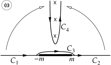
Figure 17: Contours in the $\omega$-plane used in the calculation of the thermal, Hartle–Hawking and Unruh Green’s functions.

In the second term in Eq. (B.28), due to the antisymmetry of $Q(\omega)$, the only contribution comes from the half-residue at $\omega=0$ and is equal to

$$\mathcal{G}_{th}^{(2)}=\frac{\lambda}{4\pi m}{\rm e}^{-m|x-x^{\prime}|}\approx\frac{\lambda}{4\pi}\bigg{(}\frac{1}{m}-|x-x^{\prime}|\bigg{)}\;.$$ (B.30)

Combining with Eq. (B.29), we obtain

$$\mathcal{G}_{th}\big{|}^{\rm close}=-\frac{1}{4\pi}\mathop{\rm ln}\nolimits\big{[}2\mathop{\rm ch}\nolimits{\lambda(x-x^{\prime})}-2\mathop{\rm ch}\nolimits{\lambda t}\big{]}+\frac{\lambda}{4\pi m}\;.$$ (B.31)

Recall that this result has been derived under the assumption of spacelike separation, ${|x-x^{\prime}|>|t|}$. The continuation inside the future and past light-cones is straightforward and is implemented by adding $+i\epsilon$ to the argument of the logarithm. Finally, representing the difference of the hyperbolic cosines as the product of sines, we arrive at our final result for the thermal Green’s function,

$$\mathcal{G}_{th}\big{|}^{\rm close}=-\frac{1}{4\pi}\mathop{\rm ln}\nolimits\left[4\mathop{\rm sh}\nolimits\bigg{(}\frac{\lambda}{2}(x-x^{\prime}-t)\bigg{)}\mathop{\rm sh}\nolimits\bigg{(}\frac{\lambda}{2}(x-x^{\prime}+t)\bigg{)}+i\epsilon\right]+\frac{\lambda}{4\pi m}\;.$$ (B.32)

Notice the large constant piece inversely proportional to the mass in this expression. Its appearance is a peculiarity of two dimensions where the integrals for the Green’s function are infrared divergent in the massless limit. Finite mass regulates this divergence.

We return to the remaining contributions in the Hartle–Hawking Green’s function (B.25). Using the expressions (B.8) for $\beta_{\omega}$ and $\gamma_{\omega}$, we notice that the integrals are saturated at $\omega\sim m\ll\lambda$. Expanding $Q(\omega)$ in this limit, we obtain

$$\mathcal{G}_{HH}^{(2)}\big{|}^{\rm close}_{\rm right}=-\lambda\int_{m}^{\infty}\frac{d\omega}{4\pi^{2}k\omega}\cdot\frac{\omega-k}{\omega+k}\big{(}{\rm e}^{ik(x+x^{\prime})}+{\rm e}^{-ik(x+x^{\prime})}\big{)}+\lambda\int_{0}^{m}\frac{d\omega}{\pi^{2}m^{2}}{\rm e}^{-\varkappa(x+x^{\prime})}\;.$$

We proceed similarly to the case of the thermal Green’s function above. Namely, we flip the sign of $\omega$ in the integral containing ${\rm e}^{-ik(x+x^{\prime})}$; notice that we obtain the integrals along the contours ${\cal C}_{1}$ and ${\cal C}_{2}$ of the same analytic function, with $k(\omega)$ analytically continued through the upper half-plane; add and subtract the integral along ${\cal C}_{3}$; deform the union of the contours ${\cal C}_{1}+{\cal C}_{3}+{\cal C}_{2}$ into the upper half-plane (this is allowed because $x+x^{\prime}$ is positive). The latter contour now does not encounter any singularities, so the integral along it vanishes. We are left with

$$\mathcal{G}_{HH}^{(2)}\big{|}^{\rm close}_{\rm right} =\lambda\int_{{\cal C}_{3}}\frac{d\omega}{4\pi^{2}i\omega\varkappa}\cdot\frac{\omega-i\varkappa}{\omega+i\varkappa}{\rm e}^{-\varkappa(x+x^{\prime})}+\lambda\int_{0}^{m}\frac{d\omega}{\pi^{2}m^{2}}{\rm e}^{-\varkappa(x+x^{\prime})}$$

$$=\frac{\lambda}{4\pi m}{\rm e}^{-m(x+x^{\prime})}\;,$$ (B.33)

where again only the half-residue at $\omega=0$ contributes.

Combining Eqs. (B.32) and (B.33), we obtain the Hartle–Hawking Green’s function in the right region. It is convenient to write it in two limits,

$$\begin{split}\mathcal{G}_{HH}\big{|}^{\rm close}_{\rm right}=&-\frac{1}{4\pi}\mathop{\rm ln}\nolimits\left[4\mathop{\rm sh}\nolimits\bigg{(}\frac{\lambda}{2}(x-x^{\prime}-t)\bigg{)}\mathop{\rm sh}\nolimits\bigg{(}\frac{\lambda}{2}(x-x^{\prime}+t)\bigg{)}+i\epsilon\right]\\ &+\begin{cases}-\frac{\lambda}{4\pi}(x+x^{\prime})+\frac{\lambda}{2\pi m}~{},&x+x^{\prime}\ll m^{-1}\\ \frac{\lambda}{4\pi m}~{},&x+x^{\prime}\gg m^{-1}\end{cases}\end{split}$$ (B.34)

Left region $x,x^{\prime}<0$.

Using the asymptotics of the modes, we obtain

$$\mathcal{G}_{HH}\big{|}_{\rm left}=\int_{0}^{\infty}\frac{d\omega}{4\pi\omega}\big{[}2\cos\omega(x-x^{\prime})+\beta_{\omega}{\rm e}^{-i\omega(x+x^{\prime})}+\beta^{*}_{\omega}{\rm e}^{i\omega(x+x^{\prime})}\big{]}Q(\omega)\;.$$ (B.35)

We again assume $|x-x^{\prime}|>|t|$, keeping in mind that we can always analytically continue to $|t|<|x-x^{\prime}|$ by the $i\epsilon$-prescription. The calculation is very similar to the one described in the previous paragraph, so we only briefly outline it here, without going into details. One uses the expression (B.8) for $\beta_{\omega}$ and separates Eq. (B.35) into the integrals over $0<\omega<m$ and $m<\omega$. One further rewrites the second integral as the sum of integrals over the contours ${\cal C}_{1}$ and ${\cal C}_{2}$ (see Fig. 17) of a single analytic function decreasing into the upper half-plane. Upon adding and subtracting the integral over ${\cal C}_{3}$, one deforms the contour into ${\cal C}_{4}$ to pick up the residues at the poles of the thermal factor $Q(\omega)$. In this way one arrives at

$$\begin{split}\mathcal{G}_{HH}\big{|}_{\rm left}\!=&-\frac{1}{4\pi}\mathop{\rm ln}\nolimits\Big{[}1\!-\!2{\rm e}^{-\lambda|x-x^{\prime}|}\mathop{\rm ch}\nolimits{\lambda t}\!+\!{\rm e}^{-2\lambda|x-x^{\prime}|}\Big{]}\!-\!\!\int_{{\cal C}_{3}}\!\frac{d\omega}{4\pi\omega}\bigg{[}{\rm e}^{i\omega|x-x^{\prime}|}+\frac{\omega\!-\!i\varkappa}{\omega\!+\!i\varkappa}{\rm e}^{-i\omega(x+x^{\prime})}\bigg{]}Q(\omega)\\ &+\int_{0}^{m}\frac{d\omega}{4\pi\omega}\bigg{[}2\cos{\omega|x-x^{\prime}|}+\frac{\omega-i\varkappa}{\omega+i\varkappa}{\rm e}^{-i\omega(x+x^{\prime})}+\frac{\omega+i\varkappa}{\omega-i\varkappa}{\rm e}^{i\omega(x+x^{\prime})}\bigg{]}Q(\omega)\;.\end{split}$$

The two integrals in the last formula almost cancel each other, up to a half-residue at $\omega=0$. Evaluating this residue, one obtains the final result

$$\mathcal{G}_{HH}\big{|}_{\rm left}=-\frac{1}{4\pi}\mathop{\rm ln}\nolimits\left[4\mathop{\rm sh}\nolimits\!\bigg{(}\frac{\lambda}{2}(x-x^{\prime}-t)\!\bigg{)}\mathop{\rm sh}\nolimits\!\bigg{(}\frac{\lambda}{2}(x-x^{\prime}+t)\!\bigg{)}\!+\!i\epsilon\right]-\frac{\lambda}{4\pi}(x+x^{\prime})+\frac{\lambda}{2\pi m}\,,$$ (B.36)

where $i\epsilon$ has been inserted to ensure the analytic continuation. Note that this expression is the same as the upper case in Eq. (B.34). Note also that it is valid without any restrictions on $|x+x^{\prime}|$, $|x-x^{\prime}|$, $|t|$ provided $x$ and $x^{\prime}$ are in the near-horizon region (i.e., they satisfy the condition (B.12)). If we keep $x^{\prime}$ fixed and send $x$ to $-\infty$, the Green’s function goes to a constant,

$$\mathcal{G}_{HH}\big{|}_{\rm left}\to\frac{\lambda}{2\pi}\big{(}m^{-1}-x^{\prime}\big{)}~{},\qquad\qquad x\to-\infty.$$ (B.37)

This reflects the regularity of the Hartle–Hawking state at the BH horizon.

B.2.3 Unruh Green’s function

Right region $x,x^{\prime}>0$.

A convenient way to compute the Unruh Green’s function on the right is to relate it to the Boulware Green’s function. Using Eq. (2.35) and the modes’ asymptotics (2.16), (2.18), we obtain

$$\begin{split}\mathcal{G}_{U}\big{|}_{\rm right}\!=\mathcal{G}_{B}\big{|}_{\rm right}\!+\!\int_{m}^{\infty}\!\!\dfrac{d\omega}{2\pi\omega}|\gamma_{\omega}|^{2}\dfrac{\cos[k(x\!-\!x^{\prime})\!-\!\omega t]}{{\rm e}^{2\pi\omega/\lambda}-1}+\!\int_{0}^{m}\!\!\dfrac{d\omega}{2\pi\omega}|\gamma_{\omega}|^{2}\dfrac{\cos{\omega t}}{{\rm e}^{2\pi\omega/\lambda}\!-\!1}{\rm e}^{-\varkappa(x+x^{\prime})}.\end{split}$$ (B.38)

Let us assume $x-x^{\prime}-t>0$ and compute the second term. Using the expression (B.8) for $\gamma_{\omega}$ and performing analytic continuation in $\omega$, we can write it in the form

$$\mathcal{G}_{U}^{(2)}\big{|}_{\rm right}=\int\limits_{{\cal C}_{1}+{\cal C}_{2}}\frac{d\omega\,\omega}{\pi(\omega+k)^{2}}\cdot\frac{{\rm e}^{ik(x-x^{\prime})-i\omega t}}{1-{\rm e}^{-2\pi\omega/\lambda}}-\int_{m}^{\infty}\frac{d\omega\,\omega}{\pi(\omega+k)^{2}}{\rm e}^{ik(x-x^{\prime})-i\omega t},$$ (B.39)

where the contours ${\cal C}_{1}$ and ${\cal C}_{2}$ are shown in Fig. 17. Next, we complete the first integral with the contour ${\cal C}_{3}$ and deform it into the upper half-plane, picking up the poles at $\omega=i\lambda n$. In the second integral we split the integration domain by introducing a separation scale $m\ll\omega_{1}\ll|x-x^{\prime}|^{-1},|t|^{-1}$. This yields

$$\begin{split}\mathcal{G}_{U}^{(2)}\big{|}_{\rm right}^{\rm close}=&-\frac{1}{4\pi}\mathop{\rm ln}\nolimits\big{[}1-{\rm e}^{-\lambda(x-x^{\prime}-t)}\big{]}-\int_{-m}^{m}\frac{d\omega\,\omega}{\pi(\omega+i\varkappa)^{2}}\cdot\frac{{\rm e}^{-\varkappa(x-x^{\prime})-i\omega t}}{1-{\rm e}^{-2\pi\omega/\lambda}}\\ &-\int_{m}^{\omega_{1}}\frac{d\omega\,\omega}{\pi(\omega+k)^{2}}\,{\rm e}^{ik(x-x^{\prime})-i\omega t}-\int_{\omega_{1}}^{\infty}\frac{d\omega\,\omega}{\pi(\omega+k)^{2}}\,{\rm e}^{ik(x-x^{\prime})-i\omega t}\;.\end{split}$$ (B.40)

Now we can simplify the integrands. In the integral in the first line we expand the exponents at small $\omega$. As the leading term is enhanced by the large ratio $\lambda/\omega$, we keep subleading terms to retain $\mathcal{O}(1)$-contributions. In the first integral in the second line we set the exponent to $1$. Whereas in the last integral we use the approximation $k\approx\omega$. After these simplifications the evaluation of the integrals is straightforward and we arrive at

$$\mathcal{G}_{U}^{(2)}\big{|}_{\rm right}^{\rm close}=-\frac{1}{4\pi}\mathop{\rm ln}\nolimits\bigg{[}\frac{2\mathop{\rm sh}\nolimits\frac{\lambda}{2}(x-x^{\prime}-t)}{m(x-x^{\prime}-t)}\bigg{]}+\frac{\lambda}{3\pi^{2}m}-\frac{\mathop{\rm ln}\nolimits 2-\gamma_{E}}{4\pi}+\frac{1}{16\pi}\;.$$ (B.41)

The calculation at $x-x^{\prime}-t<0$ proceeds in a similar way and gives the same result.

We still have to evaluate the last term in Eq. (B.38). Clearly, this term vanishes if $x+x^{\prime}\gg m^{-1}$. In the opposite limit, $x+x^{\prime}\ll m^{-1}$, we expand the integrand to subleading order and after an elementary integration obtain

$$\mathcal{G}_{U}^{(3)}\big{|}_{\rm right}=\begin{cases}\frac{\lambda}{\pi^{2}m}-\frac{\lambda(x+x^{\prime})}{4\pi}-\frac{1}{2\pi}~{},&x+x^{\prime}\ll m^{-1}\\ 0~{},&x+x^{\prime}\gg m^{-1}\end{cases}$$ (B.42)

Combining together the expression (B.17) for the Boulware Green’s function and Eqs. (B.41), (B.42), we end up with

$$\begin{split}\mathcal{G}_{U}\big{|}_{\rm right}^{\rm close}=&-\frac{1}{4\pi}\mathop{\rm ln}\nolimits\left[2\mathop{\rm sh}\nolimits\left(\frac{\lambda}{2}(x-x^{\prime}-t)\right)m(x-x^{\prime}+t)+i\epsilon\right]\\ &+\begin{cases}-\frac{\lambda}{4\pi}(x+x^{\prime})+\frac{4\lambda}{3\pi^{2}m}+\frac{\mathop{\rm ln}\nolimits 2-\gamma_{E}}{4\pi}-\frac{3}{16\pi}~{},&x+x^{\prime}\ll m^{-1}\\ \frac{\lambda}{3\pi^{2}m}+\frac{\mathop{\rm ln}\nolimits 2-\gamma_{E}}{4\pi}+\frac{1}{16\pi}~{},&x+x^{\prime}\gg m^{-1}\end{cases}\end{split}$$ (B.43)

We observe that the Unruh Green’s function is a mixture of the thermal right-moving and vacuum left-moving contributions. It is important to note, however, that this mixture is not a simple linear superposition: the nonsingular part in $\mathcal{G}_{U}$ is not an arithmetic mean of the nonsingular parts of $\mathcal{G}_{HH}$ and $\mathcal{G}_{B}$. In particular, the large terms $\propto\lambda/m$ produced by soft modes with $\omega\sim m$ have different coefficients in Eqs. (B.43) and (B.34). These terms play the key role in determining the tunneling solution and the vacuum decay probability in the model studied in the main text.

Note that an enhanced $\mathcal{O}(\lambda/m)$-term is present in $\mathcal{G}_{U}$ even far away from the BH implying that the soft modes are still highly populated in the asymptotic region. This is a feature of two dimensions: the radiation emitted by the BH does not spread out and persists as a constant flux of particles at arbitrarily large distance from the horizon.

Finally, the leading corrections to the expression (B.43) come from the last term in (B.38) and the second term in (B.40) and are of order ${{\cal O}\big{(}\lambda m(x\!-\!x^{\prime})^{2},\lambda mt^{2},\lambda m(x\!-\!x^{\prime})t\big{)}}$. Requiring that these corrections are smaller than the ${\cal O}(1)$ terms kept in Eq. (B.43) restricts the domain of validity of this formula to

$$|x-x^{\prime}|,~{}|t|\ll 1/\sqrt{\lambda m}\;.$$ (B.44)

Left region $x,x^{\prime}<0$.

Here it is convenient to relate the Unruh Green’s function to the Hartle–Hawking Green’s function. Upon using the mode asymptotics, we get

$$\mathcal{G}_{U}\big{|}_{\rm left}=\mathcal{G}_{HH}\big{|}_{\rm left}-\int_{m}^{\infty}\dfrac{d\omega\,k}{2\pi\omega^{2}}\,|\gamma_{\omega}|^{2}\,\dfrac{\cos[\omega(x-x^{\prime}+t)]}{{\rm e}^{2\pi\omega/\lambda}-1}\;.$$ (B.45)

Evaluation of the additional integral proceeds in complete analogy with the calculation of $\mathcal{G}_{U}^{(2)}\big{|}_{\rm right}$ above. We do not repeat this calculation, and just give the result,

$$\mathcal{G}_{U}^{(2)}\big{|}_{\rm left}^{\rm close}=\frac{1}{4\pi}\mathop{\rm ln}\nolimits\bigg{[}\frac{2\mathop{\rm sh}\nolimits\frac{\lambda}{2}(x-x^{\prime}+t)}{m(x-x^{\prime}+t)}\bigg{]}+\frac{\lambda}{m}\bigg{(}-\frac{1}{2\pi}+\frac{4}{3\pi^{2}}\bigg{)}+\frac{\mathop{\rm ln}\nolimits 2-\gamma_{E}}{4\pi}-\frac{3}{16\pi}\;.$$ (B.46)

Combining with Eq. (B.36) we obtain the final answer,

$$\begin{split}\mathcal{G}_{U}\big{|}_{\rm left}^{\rm close}=-\frac{1}{4\pi}\mathop{\rm ln}\nolimits\left[2\mathop{\rm sh}\nolimits\bigg{(}\!\frac{\lambda}{2}(x\!-\!x^{\prime}\!-\!t)\!\bigg{)}m(x\!-\!x^{\prime}\!+\!t)\!+\!i\epsilon\right]\!-\!\frac{\lambda(x\!+\!x^{\prime})}{4\pi}\!+\!\frac{4\lambda}{3\pi^{2}m}\!+\!\frac{\mathop{\rm ln}\nolimits 2\!-\!\gamma_{E}}{4\pi}\!-\!\frac{3}{16\pi}\;.\end{split}$$ (B.47)

The leading corrections to this formula are of order ${\cal O}\big{(}\lambda m(x-x^{\prime}+t)^{2}\big{)}$. On the other hand, there are no corrections in $(x-x^{\prime}-t)$. This is clear from the representation (B.45) and the fact that the form (B.36) of the Hartle–Hawking Green’s function is valid in the entire near-horizon region. Thus, the expressions (B.47) can be used as long as

$$|x-x^{\prime}+t|\ll 1/\sqrt{\lambda m}\;.$$

As expected, Eq. (B.47) coincides with the expression for $\mathcal{G}_{U}\big{|}_{\rm right}^{\rm close}$ at $x+x^{\prime}\ll m^{-1}$ (upper case in Eq. (B.43)).

Appendix C Boundary conditions for the bounce

Here we derive the boundary conditions for the bounce solution formulated in Sec. 2.4. The path integral for the false vacuum decay probability (2.40) contains the elements of the density matrix in the configuration-space basis, $\langle\varphi_{i},t_{i}^{\rm up}|\varrho|\varphi_{i}^{\prime},t_{i}^{\rm low}\rangle$. It is convenient to switch to the (over-complete) basis of coherent states

$$|a\rangle=\exp\Big{\{}\int_{0}^{\infty}d\omega\sum_{I=R,L}\Big{[}-\tfrac{1}{2}|a_{I,\omega}|^{2}+a_{I,\omega}\hat{a}_{I,\omega}^{\dagger}\Big{]}\Big{\}}|0\rangle_{B}\;.$$ (C.1)

They are eigenstates of the annihilation operator,

$$\hat{a}_{I,\omega}|a\rangle=a_{I,\omega}|a\rangle~{},~{}~{}~{}~{}~{}~{}I=R,L\;,$$ (C.2)

and provide a decomposition of unity,

$$\int D[a]D[a^{*}]\;|a\rangle\langle a|=\mathbbm{1}\;.$$ (C.3)

Therefore, the matrix element of interest takes the form

$$\langle\varphi_{i},t_{i}|\varrho|\varphi_{i}^{\prime},t_{i}^{\prime}\rangle=\int D[a]D[a^{*}]D[a^{\prime}]D[a^{\prime*}]\langle\varphi_{i},t_{i}|a\rangle\langle a|\varrho|a^{\prime}\rangle\langle a^{\prime}|\varphi_{i}^{\prime},t_{i}^{\prime}\rangle\;.$$ (C.4)

We now compute the elements entering into this formula.

In Boulware, Hartle–Hawking and Unruh vacua different modes are populated incoherently, according to the thermal distribution. Their temperature $T_{I}$ is either equal to the BH temperature $\lambda/(2\pi)$ or is zero (the mode is in vacuum). The single-mode thermal density matrix is

$$\varrho_{I,\omega}=\sum_{n}\frac{(\hat{a}^{\dagger}_{I,\omega})^{n}}{\sqrt{n!}}|0\rangle\langle 0|\frac{(\hat{a}_{I,\omega})^{n}}{\sqrt{n!}}{\rm e}^{-n\omega/T_{I}}$$ (C.5)

and its elements in the coherent-state representation are easily calculated,

$$\langle a|\varrho_{I,\omega}|a^{\prime}\rangle=\exp\Big{\{}-\tfrac{1}{2}|a_{I,\omega}|^{2}-\tfrac{1}{2}|a^{\prime}_{I,\omega}|^{2}+{\rm e}^{-\omega/T_{I}}a^{*}_{I,\omega}a^{\prime}_{I,\omega}\Big{\}}.$$ (C.6)

The total density matrix is obtained as the product of single-mode density matrices over all modes. For all states of interest the result has the general form

$$\langle a|\varrho|a^{\prime}\rangle=\exp\Big{\{}\int_{0}^{\infty}d\omega\sum_{I=R,L}\Big{[}-\tfrac{1}{2}|a_{I,\omega}|^{2}-\tfrac{1}{2}|a^{\prime}_{I,\omega}|^{2}+r_{I}(\omega)a^{*}_{I,\omega}a^{\prime}_{I,\omega}\Big{]}\Big{\}}\;,$$ (C.7)

and the difference between the Boulware, Hartle–Hawking and Unruh states is encapsulated by the coefficients $r_{I}(\omega)$, whose values are given in Eqs. (2.43).

Next, we need the wavefunction of the coherent state, $\langle\varphi_{i},t_{i}|a\rangle$. To this aim, we derive a set of differential equations that this wavefunction obeys. We notice that the annihilation and creation operators can be represented as

$$\hat{a}_{I,\omega}={\rm e}^{i\omega t_{i}}\int\frac{dx}{\sqrt{4\pi}}f^{*}_{I,\omega}(x)\bigg{(}\frac{\sqrt{\omega}}{{\rm g}}\hat{\varphi}(t_{i},x)+\frac{i{\rm g}}{\sqrt{\omega}}\hat{\pi}(t_{i},x)\bigg{)},$$ (C.8a)

$$\hat{a}_{I,\omega}^{\dagger}={\rm e}^{-i\omega t_{i}}\int\frac{dx}{\sqrt{4\pi}}f_{I,\omega}(x)\bigg{(}\frac{\sqrt{\omega}}{{\rm g}}\hat{\varphi}(t_{i},x)-\frac{i{\rm g}}{\sqrt{\omega}}\hat{\pi}(t_{i},x)\bigg{)},$$ (C.8b)

where

$$\hat{\pi}(t,x)={\rm g}^{-2}\partial_{t}\varphi(t,x)$$ (C.9)

is the canonical momentum operator. It acts by derivative on the configuration-space wavefunctions,

$$\langle\varphi_{i},t_{i}|\hat{\pi}(t_{i},x)|\psi\rangle=-i\frac{\delta}{\delta\varphi_{i}(x)}\langle\varphi_{i},t_{i}|\psi\rangle$$ (C.10)

for any quantum state $|\psi\rangle$. Hence, we can write

$$a_{I,\omega}\langle\varphi_{i},t_{i}|a\rangle=\langle\varphi_{i},t_{i}|\hat{a}_{I,\omega}|a\rangle={\rm e}^{i\omega t_{i}}\int\frac{dx}{\sqrt{4\pi}}f_{I,\omega}^{*}(x)\bigg{[}\frac{\sqrt{\omega}}{{\rm g}}\varphi_{i}(x)+\frac{{\rm g}}{\sqrt{\omega}}\frac{\delta}{\delta\varphi_{i}(x)}\bigg{]}\langle\varphi_{i},t_{i}|a\rangle\;,$$ (C.11a)

$$\bigg{[}\frac{\delta}{\delta a_{I,\omega}}\!+\!\frac{1}{2}a^{*}_{I,\omega}\bigg{]}\!\langle\varphi_{i},t_{i}|a\rangle\!=\!\langle\varphi_{i},t_{i}|\hat{a}_{I,\omega}^{\dagger}|a\rangle\!=\!{\rm e}^{-i\omega t_{i}}\!\!\int\!\!\frac{dx}{\sqrt{4\pi}}f_{I,\omega}(x)\!\bigg{[}\frac{\sqrt{\omega}}{{\rm g}}\varphi_{i}(x)\!-\!\frac{{\rm g}}{\sqrt{\omega}}\frac{\delta}{\delta\varphi_{i}(x)}\bigg{]}\!\langle\varphi_{i},t_{i}|a\rangle,$$ (C.11b)

$$\bigg{[}\frac{\delta}{\delta a^{*}_{I,\omega}}+\frac{1}{2}a_{I,\omega}\bigg{]}\langle\varphi_{i},t_{i}|a\rangle=0\;.$$ (C.11c)

The solution of this system is straightforward and yields the following result:

$$\begin{split}\langle\varphi_{i},t_{i}|a\rangle\propto\exp\Big{\{}&-\tfrac{1}{2{\rm g}^{2}}\int dxdx^{\prime}\,A(x,x^{\prime})\varphi_{i}(x)\varphi_{i}(x^{\prime})\\ &+\tfrac{1}{{\rm g}}\int d\omega dx\,\sqrt{\omega/\pi}\sum_{I}f_{I,\omega}(x)\varphi_{i}(x)a_{I,\omega}{\rm e}^{-i\omega t_{i}}\\ &-\tfrac{1}{2}\int d\omega\Big{[}\sum_{I}|a_{I,\omega}|^{2}+\sum_{I,J}B_{IJ}a_{I,\omega}a_{J,\omega}{\rm e}^{-2i\omega t_{i}}\Big{]}\Big{\}},\end{split}$$ (C.12)

where

$$A(x,x^{\prime})=\int\frac{d\omega}{2\pi}\,\omega\sum_{I}f_{I,\omega}(x)f^{*}_{I,\omega}(x^{\prime})\;,$$ (C.13a)

$$2\pi B_{IJ}\,\delta(\omega-\omega^{\prime})=\int dx\,f_{I,\omega}(x)f_{J,\omega}(x)\;.$$ (C.13b)

Note the absence of complex conjugation in the expression for $B_{IJ}$. Though Eq. (C.12) looks lengthy, its structure is simple: it is just an exponent of a quadratic form in the field $\varphi_{i}$ and the mode amplitudes $a_{I,\omega}$.

We are now ready to combine Eqs. (C.7), (C.12) and substitute them into the path integral for the decay probability. The integrals over $\varphi_{i}$, $a$, $a^{*}$ and their primed counterparts are Gaussian and hence are saturated by the saddle point. The saddle-point condition obtained by variation with respect to $\varphi_{i}(x)$, $a_{I,\omega}$, $a_{I,\omega}^{*}$ are

$$i\frac{\delta S[\varphi_{\rm b}]}{\delta\varphi_{i}(x)}\!-\!\frac{1}{{\rm g}^{2}}\int dx^{\prime}\,A(x,x^{\prime})\varphi_{i}(x^{\prime})\!+\!\frac{1}{{\rm g}}\int d\omega\sqrt{\frac{\omega}{\pi}}\sum_{I}f_{I,\omega}(x)a_{I,\omega}{\rm e}^{-i\omega t_{i}^{\rm up}}=0\;,$$ (C.14a)

$$\frac{1}{{\rm g}}\sqrt{\frac{\omega}{\pi}}\int dx\,f_{I,\omega}(x)\varphi_{i}(x){\rm e}^{-i\omega t_{i}^{\rm up}}-\sum_{J}B_{IJ}a_{J,\omega}{\rm e}^{-2i\omega t_{i}^{\rm up}}-a^{*}_{I,\omega}=0\;,$$ (C.14b)

$$-a_{I,\omega}+r_{I}(\omega)\,a^{\prime}_{I,\omega}=0\;.$$ (C.14c)

Next, we notice that the variation of the action evaluated on the bounce solution with respect to the initial value of the field is the initial momentum, taken with minus sign,

$$\frac{\delta S[\varphi_{\rm b}]}{\delta\varphi_{i}(x)}=-\pi(t_{i}^{\rm up},x)=-{\rm g}^{-2}\partial_{t}\varphi_{\rm b}(t_{i}^{\rm up},x)\;.$$ (C.15)

Substituting this into Eq. (C.14a) and performing a series of straightforward manipulations, one arrives to a very simple relation

$$c_{I,\omega}^{\rm up}=a_{I,\omega}\;,$$ (C.16a)

where $$c_{I,\omega}^{\rm up} {\cal C}$$ are the positive-frequency amplitudes of the bounce solution on the upper side of the contour (see Eq. (2.41) and Fig. 4). Inserting this result into Eq. (C.14b) leads once more to a massive simplification and yields

$$\bar{c}_{I,\omega}^{\rm up}=a_{I,\omega}^{*}\;,$$ (C.16b)

where $\bar{c}_{I,\omega}^{\rm up}$ are the negative-frequency amplitudes of the bounce on the upper side of the contour. The third equation (C.14c) is left as it is.

The saddle-point conditions following from variation with respect to the primed variables are handled in exactly the same manner. They read

$$c_{I,\omega}^{\rm low}=a^{\prime}_{I,\omega}~{},~{}~{}~{}~{}\bar{c}_{I,\omega}^{\rm low}=a^{\prime*}_{I,\omega}~{},~{}~{}~{}~{}r_{I}(\omega)\,a^{*}_{I,\omega}=a^{\prime*}_{I,\omega}\;,$$ (C.17)

where $c_{I,\omega}^{\rm low}$, $\bar{c}_{I,\omega}^{\rm low}$ are the positive- and negative-frequency amplitudes of the bounce on the lower part of the contour ${\cal C}$. Eliminating $a$, $a^{*}$, $a^{\prime}$, $a^{\prime*}$ from Eqs. (C.14c), (C.16), (C.17), we arrive at the boundary conditions (2.42) from the main text.

Finally, let us work out the initial state contribution into the tunneling exponent. This is given by the saddle-point value of the density matrix. As discussed above, both the matrix elements $\langle a|\varrho|a^{\prime}\rangle$ and the wavefunction $\langle\varphi_{i},t_{i}|a\rangle$ are exponents of homogeneous quadratic forms in $\varphi_{i}$ and $a$. On the other hand, the bounce action $S[\varphi_{\rm b}]$ is linear in $\varphi_{i}$, $\varphi_{i}^{\prime}$. Hence, the evaluation of all Gaussian integrals in the initial state variables leaves behind a simple expression,

$$\langle\varphi_{i},t_{i}^{\rm up}|\varrho|\varphi_{i}^{\prime},t_{i}^{\rm low}\rangle\big{|}_{\rm saddle}\propto\exp\bigg{\{}\int dx\bigg{[}-\frac{i}{2}\varphi_{i}(x)\frac{\delta S[\varphi_{\rm b}]}{\delta\varphi_{i}(x)}-\frac{i}{2}\varphi^{\prime}_{i}(x)\frac{\delta S[\varphi_{\rm b}]}{\delta\varphi^{\prime}_{i}(x)}\bigg{]}\bigg{\}}$$ (C.18)

This gives Eq. (2.52) upon using the relation (C.15).

Appendix D Calculation of the bounce suppression

Periodic instanton in flat space.

The suppression of the periodic instanton in flat space is given by Eq. (2.53) where one should substitute the inner core of the instanton (3.24). As discussed in the main text, the integration can be performed over the contour ${\cal C}^{\prime}$ consisting of two semi-infinite rays with $-\infty<\mathop{\rm Re}\nolimits t<0$, $\mathop{\rm Im}\nolimits t=\pm\pi/\lambda$ and a piece of imaginary time axis $\mathop{\rm Re}\nolimits t=0$, $-\pi/\lambda<\mathop{\rm Im}\nolimits t<\pi/\lambda$ connecting them, see Fig. 7a. The integrals over the rays cancel each other due to the periodicity of the solution in imaginary time. Thus, we are left with an integral over one period of the instanton in Euclidean time:

$$B_{th}=\frac{1}{{\rm\text{g}}^{2}}\!\!\int\limits_{-\pi/\lambda}^{\pi/\lambda}\!\!d\tau\!\int\limits_{-\infty}^{\infty}\!\!dx\;\frac{\lambda^{2}b_{th}}{\big{(}\mathop{\rm ch}\nolimits\lambda x\!-\!\sqrt{1\!-\!b_{th}}\cos\lambda\tau\big{)}^{2}}\Bigg{\{}\!\mathop{\rm ln}\nolimits\left[\frac{\lambda^{2}b_{th}{\rm e}^{-2\lambda x}}{\kappa\big{(}\mathop{\rm ch}\nolimits\lambda x\!-\!\sqrt{1\!-\!b_{th}}\cos\lambda\tau\big{)}^{2}}\right]\!-\!2\!+\!2\lambda x\Bigg{\}},$$ (D.1)

where we have added and subtracted a linear piece $2\lambda x$ in the square brackets. Because of the symmetry of the first factor under $x\mapsto-x$, the integral of this linear piece vanishes, so we omit it in what follows. Next, we make a change of variables

$$\mathcal{T}={\rm e}^{\lambda x}\sin{\lambda\tau}~{},~{}~{}~{}~{}X={\rm e}^{\lambda x}\cos\lambda\tau\;.$$ (D.2)

Note that this is the same transformation that connects the inertial frame coordinates $(\mathcal{T},X)$ with the frame of a uniformly accelerating observer $(\tau,x)$ in the Euclidean signature. Of course, there is no physical accelerating frame in the present calculation and we are using the change of variables (D.2) simply as a mathematical tool. The domain of integration is mapped to $-\infty<\mathcal{T},X<\infty$, and the integral becomes

$$\begin{split}B_{th}=\frac{1}{{\rm\text{g}}^{2}}\!\!\int\limits_{-\infty}^{\infty}\!d\mathcal{T}\!\!\int\limits_{-\infty}^{\infty}\!dX\;\frac{4b_{th}}{\big{(}\mathcal{T}^{2}\!+\!(X\!-\!\sqrt{1\!-\!b_{th}})^{2}\!+\!b_{th}\big{)}^{2}}\Bigg{\{}\!\mathop{\rm ln}\nolimits\left[\frac{4\lambda^{2}b_{th}}{\kappa\big{(}\mathcal{T}^{2}\!+\!(X\!-\!\sqrt{1-b_{th}})^{2}\!+\!b_{th}\big{)}^{2}}\right]\!-\!2\Bigg{\}}.\end{split}$$ (D.3)

This is easily evaluated in polar coordinates centered at $\mathcal{T}=0$, $X=\sqrt{1-b_{th}}$ and yields

$$B_{th}=\frac{4\pi}{{\rm g}^{2}}\bigg{[}\mathop{\rm ln}\nolimits\bigg{(}\frac{4\lambda^{2}}{\kappa b_{th}}\bigg{)}-4\bigg{]}\;.$$ (D.4)

Upon substitution of $b_{th}$ from Eq. (3.28), we arrive at Eq. (3.30).

Hartle–Hawking bounce.

For the periodic instantons (bounces) in the vicinity of the BH we use the expression (5.2). Then the bounce action integrated by parts is

$$\begin{split}B_{HH}=&\frac{1}{{\rm g}^{2}}\int_{-\pi/\lambda}^{\pi/\lambda}d\tau\int_{-\infty}^{\infty}dx\,\Omega(x)\kappa(\varphi_{\rm b}-2){\rm e}^{\varphi_{\rm b}}\\ =&\frac{1}{\text{g}^{2}}\int_{-\pi/\lambda}^{\pi/\lambda}d\tau\int_{-\infty}^{\infty}dx\;\frac{\lambda^{2}b_{HH}}{\big{(}\mathop{\rm ch}\nolimits\lambda(x-x_{HH})-\sqrt{1-b_{HH}}\cos\lambda\tau\big{)}^{2}}\\ &\qquad\times\Bigg{\{}\mathop{\rm ln}\nolimits\left[\frac{\lambda^{2}b_{HH}{\rm e}^{-2\lambda(x-x_{HH})}}{\kappa\big{(}\mathop{\rm ch}\nolimits\lambda(x-x_{HH})-\sqrt{1-b_{HH}}\cos\lambda\tau\big{)}^{2}}\right]-2-2\lambda x_{HH}\Bigg{\}}.\end{split}$$ (D.5)

This integral is analogous to Eq. (D.1) and is computed using the same change of variables (D.2). Upon using the relation (5.5) between $b_{HH}$ and $x_{HH}$, we obtain the result (5.7) given in the main text.

Unruh bounce far from horizon.

Substituting the expression (5.19) in the general formula (2.53), we get

$$\begin{split}B_{U1}=\frac{i}{{\rm g}^{2}}&\int_{-\infty}^{\infty}dx\int_{\cal C}dt\frac{4\lambda^{2}b_{U1}}{\left(-2\lambda(v-v_{1})\mathop{\rm sh}\nolimits\left(\frac{\lambda}{2}(u-u_{1})\right)+b_{U1}{\rm e}^{\frac{\lambda}{2}(u-u_{1})}\right)^{2}}\\ &\times\left\{\mathop{\rm ln}\nolimits\left[\frac{4\lambda^{2}b_{U1}}{\kappa\left(-2\lambda(v-v_{1})\mathop{\rm sh}\nolimits\left(\frac{\lambda}{2}(u-u_{1})\right)+b_{U1}{\rm e}^{\frac{\lambda}{2}(u-u_{1})}\right)^{2}}\right]-2\right\}.\end{split}$$ (D.6)

Recall that the time integral is performed over a contour ${\cal C}$ running along the real axis and encircling the singularity of the integrand. This singularity is quite complicated: it is a second-order pole superimposed on a logarithmic branch cut. The calculation is greatly simplified by a change of variables. First, we introduce a new advanced coordinate

$$\tilde{u}=\lambda^{-1}\big{(}1-{\rm e}^{-\lambda(u-u_{1})}\big{)}\;.$$ (D.7)

Notice that when $u$ varies from $-\infty$ to $+\infty$, $\tilde{u}$ varies from $-\infty$ to $1/\lambda$. Second, we introduce new time and space variables

$$\tilde{t}=\tfrac{\lambda}{2}(v-v_{1}+\tilde{u})~{},~{}~{}~{}~{}~{}\tilde{x}=\tfrac{\lambda}{2}(v-v_{1}-\tilde{u})\;.$$ (D.8)

With this replacement the integral becomes

$$\begin{split}B_{U1}=\frac{i}{{\rm g}^{2}}\!\int\limits_{-\infty}^{\infty}\!d\tilde{x}\!\int\limits_{\tilde{\cal C}_{\tilde{x}}}\!d\tilde{t}\;\frac{4b_{U1}}{\left(-\tilde{t}^{2}\!+\!\tilde{x}^{2}\!+\!b_{U1}\right)^{2}}\left\{\mathop{\rm ln}\nolimits\left[\frac{4\lambda^{2}b_{U1}}{\kappa\left(-\tilde{t}^{2}\!+\!\tilde{x}^{2}\!+\!b_{U1}\right)^{2}}\right]\!-\!2\!+\!\mathop{\rm ln}\nolimits(1\!-\!\tilde{t}\!+\!\tilde{x})\right\}.\end{split}$$ (D.9)

The time contour $\tilde{\cal C}_{\tilde{x}}$, which is now $\tilde{x}$-dependent, runs along the real axis and encircles the singularity at $\tilde{t}=-\sqrt{\tilde{x}^{2}+b_{U1}}$, but avoids the logarithmic cut of the last term in braces at $\tilde{t}=\tilde{x}+1$, see Fig. 18. We make a crucial observation: if we restrict the integrand to the first two terms in braces, the contour can be freely deformed into the imaginary time axis. The resulting integral has the same form as in Eq. (D.3) and can be easily evaluated in polar coordinates. It leads to the same result as Eq. (D.4) with the replacement $b_{th}\mapsto b_{U1}$.

The remaining contribution is computed by residues and turns out to vanish,

$$\begin{split}&\frac{2\pi}{{\rm g}^{2}}\int_{-\infty}^{\infty}d\tilde{x}\;\frac{\partial}{\partial\tilde{t}}\bigg{[}\frac{4b_{U1}\mathop{\rm ln}\nolimits(1-\tilde{t}+\tilde{x})}{(\tilde{t}-\sqrt{\tilde{x}^{2}+b_{U1}})^{2}}\bigg{]}\bigg{|}_{\tilde{t}=-\sqrt{\tilde{x}^{2}+b_{U1}}}\\ &=\frac{2\pi}{{\rm g}^{2}}\int_{-\infty}^{\infty}d\tilde{x}\;\bigg{[}\frac{b_{U1}\mathop{\rm ln}\nolimits(1+\tilde{x}+\sqrt{\tilde{x}^{2}+b_{U1}})}{(\tilde{x}^{2}+b_{U1})^{3/2}}-\frac{b_{U1}}{(\tilde{x}^{2}+b_{U1})(1+\tilde{x}+\sqrt{\tilde{x}^{2}+b_{U1}})}\bigg{]}=0\;.\end{split}$$ (D.10)

Thus, we conclude that

$$B_{U1}=\frac{4\pi}{{\rm g}^{2}}\bigg{[}\mathop{\rm ln}\nolimits\bigg{(}\frac{4\lambda^{2}}{\kappa b_{U1}}\bigg{)}-4\bigg{]}\;,$$ (D.11)

which upon substitution of $b_{U1}$ from Eq. (5.22) yields Eq. (5.26).

Figure 18: Time integration contour in Eq. (D.9).

Unruh bounce near horizon.

Here the starting expression is

$$\begin{split}B_{U2}=\frac{i}{{\rm g}^{2}}&\int_{-\infty}^{\infty}dx\int_{\cal C}dt\frac{4\lambda^{2}b_{U2}}{\left(-2\lambda(v-v_{2})\mathop{\rm sh}\nolimits\left(\frac{\lambda}{2}(u-u_{2})\right)+b_{U2}{\rm e}^{\frac{\lambda}{2}(u-u_{2})}\right)^{2}}\\ &\times\left\{\mathop{\rm ln}\nolimits\left[\frac{4\lambda^{2}b_{U2}}{\kappa\left(-2\lambda(v-v_{2})\mathop{\rm sh}\nolimits\left(\frac{\lambda}{2}(u-u_{2})\right)+b_{U2}{\rm e}^{\frac{\lambda}{2}(u-u_{2})}\right)^{2}}\right]-2\lambda x-2\right\}.\end{split}$$ (D.12)

Upon the change of variables analogous to the previous paragraph, we obtain

$$\begin{split}B_{U2}=\frac{i}{{\rm g}^{2}}\!\int\limits_{-\infty}^{\infty}\!d\tilde{x}\!\int\limits_{\tilde{\cal C}_{\tilde{x}}}\!d\tilde{t}\;\frac{4b_{U2}}{\left(-\tilde{t}^{2}\!+\!\tilde{x}^{2}\!+\!b_{U2}\right)^{2}}\left\{\mathop{\rm ln}\nolimits\left[\frac{4\lambda^{2}b_{U2}}{\kappa\left(-\tilde{t}^{2}\!+\!\tilde{x}^{2}\!+\!b_{U2}\right)^{2}}\right]\!-\!\tilde{t}\!-\!\tilde{x}\!-\!2\lambda x_{2}\!-\!2\right\}.\end{split}$$ (D.13)

We can now deform the time integration contour into the imaginary axis and take the integral in polar coordinates. In this way we obtain

$$B_{U2}=\frac{4\pi}{{\rm g}^{2}}\bigg{[}\mathop{\rm ln}\nolimits\bigg{(}\frac{4\lambda^{2}}{\kappa b_{U2}}\bigg{)}-2\lambda x_{2}-4\bigg{]}\;,$$ (D.14)

which yields Eq. (5.37) after substituting $b_{U2}$ from Eq. (5.31).

Appendix E A failed attempt: Nonminimal coupling

Throughout the main text we consider a minimally coupled scalar field. As a result, the field equation for our toy model (4.4) is not exactly solvable, even in the massless limit, unless the metric function $\Omega$ satisfies $(\mathop{\rm ln}\nolimits\Omega)^{\prime\prime}=0$. On the other hand, it is well-known that the classical Liouville theory remains exactly solvable in an arbitrary metric if one adds a nonminimal coupling of the scalar field to curvature. In this Appendix we consider such coupling and explain why it is not suitable for our purposes.

The nonminimal coupling in question has the form

$$S_{\rm nm}=-\frac{1}{\text{g}^{2}}\int d^{2}x\sqrt{-g}\,R\varphi\;,$$ (E.1)

where $R$ is the Ricci scalar given by Eq. (4.2) for an arbitrary metric written in the conformally flat form. Notice that this coupling is linear in the field $\varphi$ and thus leads to a source term $-\Box\mathop{\rm ln}\nolimits\Omega$ on the r.h.s. of the field equation (4.4). It is straightforward to see that in the presence of this source the expression (4.5) provides the general solution for $\varphi$ in the massless limit, for an arbitrary metric function $\Omega$.

However, the presence of the source in the field equation has an unwanted consequence. It modifies the classical false vacuum by shifting it away from $\varphi=0$. To see this, we use the metric of dilaton BH (2.7). The result does not qualitatively depend on this particular choice, as long as the metric has a horizon with the temperature $\lambda\gg m$. Due to the space-dependent source the false vacuum configuration $\varphi_{\rm fv}(x)$ becomes inhomogeneous. To find it, we omit the nonlinear term in the potential and obtain the equation

$$\varphi_{\rm fv}^{\prime\prime}-m^{2}\Omega\varphi_{\rm fv}+(\mathop{\rm ln}\nolimits\Omega)^{\prime\prime}=0\;.$$ (E.2)

In the region $x\ll 1/m$ the mass term can be neglected and the solution is

$$\varphi_{\rm fv}=-\mathop{\rm ln}\nolimits\Omega+2\lambda x+C_{\rm fv}\;.$$ (E.3)

The linear term has been fixed by the regularity of the field at the horizon, $x\to-\infty$, whereas the constant term $C_{\rm fv}$ must be determined from the behavior at $x\gg 1/\lambda$. In that region the field has the usual exponential form, $\varphi_{\rm fv}=A_{\rm fv}{\rm e}^{-mx}$. Comparing to Eq. (E.3), we get $C_{\rm fv}=A_{\rm fv}=-2\lambda/m$. We see that in the near-horizon region the field acquires large negative values: $\varphi_{\rm fv}=-2\lambda/m$ at $x\to-\infty$. In other words, it is driven away from the tunneling region located at large positive $\varphi$.

It is instructive to compute the false vacuum energy. A straightforward calculation gives

$$E_{\rm fv}=-\frac{2\lambda^{2}}{{\text{g}}^{2}m}\bigg{(}1-\frac{m}{2\lambda}\bigg{)}\;,$$ (E.4)

where we have taken into account the potential energy coming from the nonminimal coupling term (E.1). We see that $E_{\rm fv}$ is negative and its absolute value grows with $\lambda$ faster than the BH temperature $T_{BH}\propto\lambda$.

To get a sense of how this property affects false vacuum decay, let us find the sphaleron energy separating the false and true vacua in the vicinity of the BH. We add the Liouville term to Eq. (E.2) and, as usual, solve it separately for the core and tail. At $x\ll 1/m$ we have

$$\varphi_{\rm sph}\Big{|}_{x\ll m^{-1}}=\mathop{\rm ln}\nolimits\left[\frac{\lambda^{2}}{\Omega(x)\kappa\mathop{\rm ch}\nolimits^{2}\lambda(x-x_{\rm sph})}\right]$$ (E.5)

with $x_{\rm sph}$ an arbitrary constant. By matching to the solution of the free massive equation at $x\gg 1/\lambda$,

$$\varphi_{\rm sph}\Big{|}_{x\gg\lambda^{-1}}=A_{\rm sph}{\rm e}^{-mx}\;,$$ (E.6)

we find

$$x_{\rm sph}=\frac{1}{m}-\frac{1}{\lambda}\mathop{\rm ln}\nolimits\frac{2\lambda}{\sqrt{\kappa}}~{},~{}~{}~{}~{}~{}A_{\rm sph}=\frac{2\lambda}{m}\;.$$ (E.7)

Note that $x_{\rm sph}$ is always smaller than $1/m$ and the matching region always exists. The sphaleron energy then reads

$$E_{\rm sph}=\frac{\lambda}{{\text{g}}^{2}}\bigg{[}8\mathop{\rm ln}\nolimits\frac{2\lambda}{\sqrt{\kappa}}-\frac{2\lambda}{m}-7\bigg{]}\;.$$ (E.8)

Thus, the energy difference between the sphaleron and the false vacuum,

$$E_{\rm sph}-E_{\rm fv}=\frac{8\lambda}{{\text{g}}^{2}}\bigg{(}\mathop{\rm ln}\nolimits\frac{\lambda}{\sqrt{\kappa}}+\mathop{\rm ln}\nolimits 2-1\bigg{)}\;,$$ (E.9)

increases with the growth of $\lambda$ and for $\lambda>\Lambda_{0}/2$ becomes bigger than the sphaleron energy in flat space, Eq. (3.11). The corresponding suppression of jumps over the sphaleron in the Hartle–Hawking state is (cf. Sec. 5.1)

$$B_{HH}=\frac{2\pi(E_{\rm sph}-E_{\rm fv})}{\lambda}=\frac{16\pi}{{\rm g}^{2}}\left(\mathop{\rm ln}\nolimits\frac{\lambda}{\sqrt{\kappa}}+\mathop{\rm ln}\nolimits 2-1\right)\;,$$ (E.10)

which is larger than the suppression in flat spacetime, Eq. (3.21) (recall that we assume $\lambda\gg m$). This means that in the theory with the nonminimal coupling transitions from the false to true vacuum in the BH vicinity are suppressed, instead of being catalyzed. In fact, the vacuum decay will be dominated by tunneling far away from the BH, in the asymptotically flat region.

In realistic situations, such as, e.g., a scalar field in the background of a Schwarzschild BH, one does not expect any modification of the classical false vacuum. Thus, we do not want this property to be present in the toy model. This is why we focus on the study of a minimally coupled scalar in this paper.

Appendix F Decay of the Boulware vacuum

In this Appendix we construct bounce solutions describing tunneling from the Boulware vacuum in the BH background. This vacuum is empty from the viewpoint of an observer at asymptotic infinity. However, the corresponding vacuum energy-momentum tensor diverges at the horizon [68] rendering this state unphysical. The problem of decay of this state is still of academic interest for comparison with the realistic cases of Hartle–Hawking and Unruh vacua. Also, the Boulware vacuum may provide an adequate description for the quantum field state in the metric of BH mimickers: horizonless compact objects with the size only slightly exceeding the gravitational radius [84] (see [85] for review).

We observe that the singular part of the Boulware Green’s function in Eqs. (B.17), (B.24) is similar to that of the Feynman function in flat spacetime. This suggests to use a linear Ansatz for the functions $F$ and $G$ in the general solution (4.5) for the bounce core. Working in the Euclidean time, we write

$$F(z)=C_{B}\,(z-x_{B})~{},~{}~{}~{}~{}~{}G(\bar{z})=C_{B}\,(\bar{z}-x_{B})\;,$$ (F.1)

where $z,\bar{z}$ are defined in Eq. (3.15) and $x_{B}$ is the coordinate of the bounce center. To determine the constant $C_{B}$, we need to match the core to the Green’s function, including the subleading nonsingular terms. This matching works differently when the bounce center is in one of the following four regions:

$$(a)~{}~{}x_{B}>0~{},~{}~{}x_{B}\gg 1/m\;, (b)~{}~{}x_{B}>0~{},~{}~{}1/\lambda\ll x_{B}\ll 1/m\;,$$

$$(c)~{}~{}x_{B}<0~{},~{}~{}1/\lambda\ll|x_{B}|\ll 1/m\;, (d)~{}~{}x_{B}<0~{},~{}~{}|x_{B}|\gg 1/m\;.$$

We consider these possibilities one after the other.

(a) In this case, the Green’s function is the same as in flat spacetime. Correspondingly, one obtains $C_{B}=C_{M}$, with $C_{M}$ given by Eq. (3.18). The tunneling suppression is also the same as in flat space, Eq. (3.21).

(b) Since $\Omega\approx 1$ in this region, the bounce core still has the same form as in flat space,

$$\varphi_{\rm b}\Big{|}_{\text{core},\;x_{B}>0}=\mathop{\rm ln}\nolimits\left[\frac{4C_{B}^{2}}{(1+\kappa C_{B}^{2}|z-x_{B}|^{2})^{2}}\right]\;.$$ (F.2)

On the other hand, the constant in the Green’s function differs from that in flat space, see the upper line in Eq. (B.17). This can be interpreted as a manifestation of the vacuum polarization by the geometry. The matching gives

$$C_{B}=\frac{m^{2}}{2\kappa}{\rm e}^{2\gamma_{E}-1}\;,$$ (F.3)

which is smaller than $C_{M}$ by a factor ${\rm e}$. The suppression is calculated in the same way as in flat space and we obtain

$$B_{B}=\frac{16\pi}{{\rm g}^{2}}\left(\mathop{\rm ln}\nolimits\frac{m}{\sqrt{\kappa}}+\gamma_{E}-\frac{3}{2}\right)\;.$$ (F.4)

This is slightly below the flat-space suppression (3.21) due to the difference in the last term. Notice, however, that the leading logarithmic part does not change.

(c) One might think that tunneling could be further enhanced in the near-horizon region. However, this does not happen, as we now show. Here the metric function is $\Omega\approx{\rm e}^{2\lambda x}$ and the bounce core gets modified,

$$\varphi_{\rm b}\Big{|}_{\text{core},\;x_{B}<0}=\mathop{\rm ln}\nolimits\left[\frac{4C_{B}^{2}}{(1+\kappa C_{B}^{2}|z-x_{B}|^{2})^{2}}\right]-2\lambda x\;.$$ (F.5)

This brings a problem: we cannot match the linear term in this expression to the expansion of the Green’s function, see the upper line in Eq. (B.24). It is straightforward to check that modifying the Ansatz (F.1) will not help. In particular, quadratic corrections added to the functions $F$ and $G$ will cancel in the long-distance asymptotics of the core, whereas the cubic ones will produce quadratic contributions in $\varphi_{\rm b}$, instead of the required linear term. We conclude that precise matching is impossible, excluding bounce solutions with the core localized in the near-horizon region.

To see this in more detail, let us perform a ‘partial’ matching assuming that the gradients of the first term in Eq. (F.5) are much larger than $\lambda$. This will hold in the matching region if the following inequalities can be simultaneously satisfied:

$$(\sqrt{\kappa}C_{B})^{-1}\ll|z-x_{B}|\ll\lambda^{-1}\;.$$ (F.6)

Then we can set $x\approx x_{B}$ in the second term in Eq. (F.5) and, comparing with the expansion of the Green’s function, we obtain

$$C_{B}=\frac{m^{2}}{2\kappa}{\rm e}^{2\gamma_{E}-1+\lambda|x_{B}|}\;.$$ (F.7)

Since $|x_{B}|\gg 1/\lambda$, this is much larger than the value of $C_{B}$ in the outer region, Eq. (F.3). Thus, our assumption (F.6) is a posteriori justified. Using the found value of $C_{B}$, we compute the bounce suppression as a function of the core position,

$$B_{B}=\frac{16\pi}{\text{g}^{2}}\left(\mathop{\rm ln}\nolimits\dfrac{m}{\sqrt{\varkappa}}+\gamma_{E}-\frac{3}{2}+\lambda|x_{B}|\right)\;.$$ (F.8)

This grows for bounces that are deeper in the near-horizon region, and decreases towards the value (F.4) when the bounce core approaches the outer boundary of this region.

(d) One can check that in this region the suppression of ‘partially matched’ bounces further increases with $|x_{B}|$. Therefore, these bounces are even further suppressed than in the region (c).

To sum up, we have found that the Boulware bounces are ‘pushed out’ from the near-horizon region and the optimal tunneling rate is achieved when the bounce center is in the region ${\it(b)}$. The corresponding suppression (F.4) is only marginally weaker than in flat spacetime.

A comment is in order. With our analytic approach we cannot exclude existence of a bounce solution with the core at $|x_{B}|\lesssim 1/\lambda$, i.e., right at the boundary between the near-horizon and the outer regions. Such solution, if it exists, can have a lower suppression than (F.4). Still, we do not expect it to differ in the first logarithmically enhanced term. A detailed investigation of this issue requires numerical analysis, which is beyond the scope of this paper.

Appendix G Hartle–Hawking sphaleron at low temperatures

Here we study the static sphaleron solution which provides a tunneling channel from the Hartle–Hawking vacuum. We focus on the BH temperatures below the critical value (5.6). Unlike in the main text, we do not assume $\lambda\gg m$. The sphaleron satisfies the equation (5.11). As usual, we will look for the solution separately in two regions. In the core (tail) we will neglect the mass (Liouville) term. Then we will glue the two solutions in the overlap.

In the inner region the form of the solution is fixed by the requirement of regularity at the horizon and is given by Eq. (5.9). It is straightforward to see that the derivation of this expression does not assume any hierarchy between $\lambda$ and $m$.

In the outer region, the sphaleron is given by the zero-frequency solution of the Schrödinger equation (2.15) vanishing at $x\to+\infty$. This is expressed in terms of the hypergeometric function,

$$\varphi_{\rm sph}=A_{HH,{\rm sph}}\,{\rm e}^{-mx}\,{}_{2}F_{1}\left(\frac{m}{2\lambda},\frac{m}{2\lambda},1+\frac{m}{\lambda}\>;-{\rm e}^{-2\lambda x}\right)\;.$$ (G.1)

Its asymptotics at large negative $x$ is inferred from Eq. (H.3),

$$\varphi_{\rm sph}\approx A_{HH,{\rm sph}}\,\frac{\Gamma\left(1+\frac{m}{\lambda}\right)}{\left[\Gamma\left(1+\frac{m}{2\lambda}\right)\right]^{2}}\bigg{[}1-mx+\frac{m}{\lambda}\bigg{(}\psi(1)-\psi\Big{(}1+\frac{m}{2\lambda}\Big{)}\bigg{)}\bigg{]}\;.$$ (G.2)

where $\psi(s)=\Gamma^{\prime}(s)/\Gamma(s)$. Matching this to the expansion of Eq. (5.9) at $(x-x_{HH,{\rm sph}})\gg 1/\lambda$, we find

$$x_{HH,{\rm sph}}=\frac{2}{m}-\frac{1}{\lambda}\mathop{\rm ln}\nolimits\dfrac{2\lambda}{\sqrt{\kappa}}+4\bigg{(}\psi(1)-\psi\Big{(}1+\frac{m}{2\lambda}\Big{)}\bigg{)}~{},~{}~{}~{}A_{HH,{\rm sph}}=\frac{4\lambda\left[\Gamma\left(1+\frac{m}{2\lambda}\right)\right]^{2}}{m\,\Gamma\left(1+\frac{m}{\lambda}\right)}\;.$$ (G.3)

Note that the expression for $x_{HH,{\rm sph}}$ reduces to Eq. (5.8) in the limit $\lambda\gg m$.

Let us compute the sphaleron energy and the associated tunneling suppression. As usual, it is convenient to integrate by parts in the expression for the energy. The boundary terms vanish, because $\varphi_{\rm sph}\partial_{x}\varphi_{\rm sph}\to 0$ both at the horizon (due to the vanishing of $\partial_{x}\varphi_{\rm sph}$) and at infinity. Then for the energy we obtain

$$\begin{split}E_{\rm sph}=\frac{1}{\text{g}^{2}}\!\int\limits_{-\infty}^{\infty}\!dx\;\Omega(x)\kappa(\varphi_{\rm sph}\!-\!2){\rm e}^{\varphi_{\rm sph}}=\frac{8\lambda}{\text{g}^{2}}\bigg{[}\!\mathop{\rm ln}\nolimits\frac{\lambda}{\sqrt{\kappa}}\!-\!\frac{\lambda}{m}\!+\!\mathop{\rm ln}\nolimits 2\!-\!1\!+\!\psi\bigg{(}\!1\!+\!\frac{m}{2\lambda}\bigg{)}\!-\!\psi(1)\bigg{]}.\end{split}$$ (G.4)

Thus, at $\lambda\lesssim\Lambda_{HH}$ the sphaleron provides a tunneling channel with the suppression

$$B_{\rm sph}=\frac{16\pi}{\text{g}^{2}}\left[\mathop{\rm ln}\nolimits\frac{\lambda}{\sqrt{\kappa}}-\frac{\lambda}{m}+\mathop{\rm ln}\nolimits 2-1+\psi\bigg{(}1+\frac{m}{2\lambda}\bigg{)}-\psi(1)\right]\;.$$ (G.5)

Using $\psi(1)=-\gamma_{E}$ and Eq. (H.1) for the asymptotics of $\psi(s)$ at large values of its argument, one can check that at $\lambda\to 0$ the expression (G.5) tends to the vacuum suppression (3.21) with the corrections starting at the quadratic order ${\cal O}(\lambda^{2}/m^{2})$. In the regime $\lambda\gg m$ it coincides with the periodic instanton action (5.7) computed in Sec. 5.1.

Appendix H Some useful formulas

Asymptotic expansion of the $\psi$-function at infinity (Eq. (5.11.2) from [86]):

$$\psi(z)\sim\mathop{\rm ln}\nolimits{z}-\frac{1}{2z}-\sum_{k=1}^{\infty}\frac{B_{2k}}{2k\,z^{2k}}\;,~{}~{}~{}~{}~{}~{}z\to\infty,~{}|\arg z|<\pi\;,$$ (H.1)

where $B_{2k}$ are the Bernoulli numbers.

Transformation of variables in the hypergeometric function (from Eqs. (15.8.2), (15.1.2) of [86]):

$$\begin{split}\frac{\sin(\pi(b\!-\!a))}{\pi\Gamma(c)}~{}_{2}F_{1}(a,b,c;z)&=\frac{(-z)^{-a}}{\Gamma(b)\Gamma(c\!-\!a)\Gamma(a\!-\!b\!+\!1)}~{}_{2}F_{1}\bigg{(}a,a\!-\!c\!+\!1,a\!-\!b\!+\!1;\frac{1}{z}\bigg{)}\\ &-\frac{(-z)^{-b}}{\Gamma(a)\Gamma(c\!-\!b)\Gamma(b\!-\!a\!+\!1)}~{}_{2}F_{1}\bigg{(}b,b\!-\!c\!+\!1,b\!-\!a\!+\!1;\frac{1}{z}\bigg{)}.\end{split}$$ (H.2)

Asymptotic expansion of the hypergeometric function when $b-a$ is a nonnegative integer (from Eqs. (15.8.8), (15.1.2) of [86]):

$$\begin{split}_{2}F_{1}&(a,a+m,c;z)=\frac{(-z)^{-a}\Gamma(c)}{\Gamma(a+m)}\sum_{k=0}^{m-1}\frac{(a)_{k}(m-k-1)!}{k!\,\Gamma(c-a-k)}z^{-k}\\ &+\frac{(-z)^{-a}\Gamma(c)}{\Gamma(a)}\sum_{k=0}^{\infty}\frac{(a+m)_{k}}{k!\,(k+m)!\,\Gamma(c-a-k-m)}(-1)^{k}z^{-k-m}\\ &\times\big{(}\mathop{\rm ln}\nolimits(-z)+\psi(k+1)+\psi(k+m+1)-\psi(a+k+m)-\psi(c-a-k-m)\big{)}\;.\end{split}$$ (H.3)

In both above equations it is assumed that $|\arg(-z)|<\pi$. In addition, in the second equation $|z|>1$, $m$ is a nonnegative integer, $(a)_{k}=a(a+1)\ldots(a+k-1)$ and $\psi(s)=\Gamma^{\prime}(s)/\Gamma(s)$.

References

- [1] W. A. Hiscock, Can black holes nucleate vacuum phase transitions?, Phys. Rev. D35 (1987) 1161.
- [2] V. A. Berezin, V. A. Kuzmin and I. I. Tkachev, O(3) Invariant Tunneling in General Relativity, Phys. Lett. B207 (1988) 397.
- [3] P. B. Arnold, Gravity and false vacuum decay rates: O(3) solutions, Nucl. Phys. B346 (1990) 160.
- [4] V. A. Berezin, V. A. Kuzmin and I. I. Tkachev, Black holes initiate false vacuum decay, Phys. Rev. D43 (1991) 3112.
- [5] R. A. Flores and M. Sher, Upper Limits to Fermion Masses in the Glashow-Weinberg-Salam Model, Phys. Rev. D 27 (1983) 1679.
- [6] M. Sher, Electroweak Higgs Potentials and Vacuum Stability, Phys. Rept. 179 (1989) 273.
- [7] G. Isidori, G. Ridolfi and A. Strumia, On the metastability of the standard model vacuum, Nucl. Phys. B 609 (2001) 387 [hep-ph/0104016].
- [8] F. Bezrukov, M. Yu. Kalmykov, B. A. Kniehl and M. Shaposhnikov, Higgs Boson Mass and New Physics, JHEP 10 (2012) 140 [1205.2893].
- [9] G. Degrassi, S. Di Vita, J. Elias-Miro, J. R. Espinosa, G. F. Giudice, G. Isidori et al., Higgs mass and vacuum stability in the Standard Model at NNLO, JHEP 08 (2012) 098 [1205.6497].
- [10] D. Buttazzo, G. Degrassi, P. P. Giardino, G. F. Giudice, F. Sala, A. Salvio et al., Investigating the near-criticality of the Higgs boson, JHEP 12 (2013) 089 [1307.3536].
- [11] A. V. Bednyakov, B. A. Kniehl, A. F. Pikelner and O. L. Veretin, Stability of the Electroweak Vacuum: Gauge Independence and Advanced Precision, Phys. Rev. Lett. 115 (2015) 201802 [1507.08833].
- [12] A. Andreassen, W. Frost and M. D. Schwartz, Scale Invariant Instantons and the Complete Lifetime of the Standard Model, Phys. Rev. D97 (2018) 056006 [1707.08124].
- [13] R. Gregory, I. G. Moss and B. Withers, Black holes as bubble nucleation sites, JHEP 03 (2014) 081 [1401.0017].
- [14] P. Burda, R. Gregory and I. Moss, Gravity and the stability of the Higgs vacuum, Phys. Rev. Lett. 115 (2015) 071303 [1501.04937].
- [15] P. Burda, R. Gregory and I. Moss, Vacuum metastability with black holes, JHEP 08 (2015) 114 [1503.07331].
- [16] P. Burda, R. Gregory and I. Moss, The fate of the Higgs vacuum, JHEP 06 (2016) 025 [1601.02152].
- [17] J. Garcia-Bellido, A. D. Linde and D. Wands, Density perturbations and black hole formation in hybrid inflation, Phys. Rev. D 54 (1996) 6040 [astro-ph/9605094].
- [18] T. Fujita, M. Kawasaki, K. Harigaya and R. Matsuda, Baryon asymmetry, dark matter, and density perturbation from primordial black holes, Phys. Rev. D 89 (2014) 103501 [1401.1909].
- [19] R. Allahverdi, J. Dent and J. Osinski, Nonthermal production of dark matter from primordial black holes, Phys. Rev. D 97 (2018) 055013 [1711.10511].
- [20] O. Lennon, J. March-Russell, R. Petrossian-Byrne and H. Tillim, Black Hole Genesis of Dark Matter, JCAP 04 (2018) 009 [1712.07664].
- [21] L. Morrison, S. Profumo and Y. Yu, Melanopogenesis: Dark Matter of (almost) any Mass and Baryonic Matter from the Evaporation of Primordial Black Holes weighing a Ton (or less), JCAP 05 (2019) 005 [1812.10606].
- [22] D. Hooper, G. Krnjaic and S. D. McDermott, Dark Radiation and Superheavy Dark Matter from Black Hole Domination, JHEP 08 (2019) 001 [1905.01301].
- [23] D. Hooper, G. Krnjaic, J. March-Russell, S. D. McDermott and R. Petrossian-Byrne, Hot Gravitons and Gravitational Waves From Kerr Black Holes in the Early Universe, 2004.00618.
- [24] V. De Luca, G. Franciolini, A. Kehagias and A. Riotto, Standard model baryon number violation seeded by black holes, Phys. Lett. B 819 (2021) 136454 [2102.07408].
- [25] B. Carr, K. Kohri, Y. Sendouda and J. Yokoyama, Constraints on Primordial Black Holes, 2002.12778.
- [26] F. R. Klinkhamer and N. S. Manton, A Saddle Point Solution in the Weinberg-Salam Theory, Phys. Rev. D 30 (1984) 2212.
- [27] W. G. Unruh, Notes on black hole evaporation, Phys. Rev. D14 (1976) 870.
- [28] J. B. Hartle and S. W. Hawking, Path Integral Derivation of Black Hole Radiance, Phys. Rev. D13 (1976) 2188.
- [29] N. Tetradis, Black holes and Higgs stability, JCAP 1609 (2016) 036 [1606.04018].
- [30] D. Gorbunov, D. Levkov and A. Panin, Fatal youth of the Universe: black hole threat for the electroweak vacuum during preheating, JCAP 1710 (2017) 016 [1704.05399].
- [31] K. Mukaida and M. Yamada, False Vacuum Decay Catalyzed by Black Holes, Phys. Rev. D96 (2017) 103514 [1706.04523].
- [32] K. Kohri and H. Matsui, Electroweak Vacuum Collapse induced by Vacuum Fluctuations of the Higgs Field around Evaporating Black Holes, Phys. Rev. D98 (2018) 123509 [1708.02138].
- [33] T. Hayashi, K. Kamada, N. Oshita and J. Yokoyama, On catalyzed vacuum decay around a radiating black hole and the crisis of the electroweak vacuum, JHEP 08 (2020) 088 [2005.12808].
- [34] D. Canko, I. Gialamas, G. Jelic-Cizmek, A. Riotto and N. Tetradis, On the Catalysis of the Electroweak Vacuum Decay by Black Holes at High Temperature, Eur. Phys. J. C78 (2018) 328 [1706.01364].
- [35] D.-C. Dai, R. Gregory and D. Stojkovic, Connecting the Higgs Potential and Primordial Black Holes, Phys. Rev. D 101 (2020) 125012 [1909.00773].
- [36] S. R. Coleman and F. De Luccia, Gravitational Effects on and of Vacuum Decay, Phys. Rev. D21 (1980) 3305.
- [37] S. W. Hawking and I. G. Moss, Supercooled Phase Transitions in the Very Early Universe, Phys. Lett. B 110 (1982) 35.
- [38] S. Tomsovic, Tunneling in Complex Systems. WORLD SCIENTIFIC, 1998, https://doi.org/10.1142/3768.
- [39] S. R. Coleman, The Fate of the False Vacuum. 1. Semiclassical Theory, Phys. Rev. D15 (1977) 2929.
- [40] C. G. Callan, Jr. and S. R. Coleman, The Fate of the False Vacuum. 2. First Quantum Corrections, Phys. Rev. D16 (1977) 1762.
- [41] S. R. Coleman, The Uses of Instantons, Subnucl. Ser. 15 (1979) 805.
- [42] W. H. Miller, Classical-limit quantum mechanics and the theory of molecular collisions, in Advances in Chemical Physics, pp. 69–177. John Wiley & Sons, Ltd, 1974.
- [43] V. A. Rubakov, D. T. Son and P. G. Tinyakov, Classical boundary value problem for instanton transitions at high-energies, Phys. Lett. B 287 (1992) 342.
- [44] G. F. Bonini, A. G. Cohen, C. Rebbi and V. A. Rubakov, The Semiclassical description of tunneling in scattering with multiple degrees of freedom, Phys. Rev. D 60 (1999) 076004 [hep-ph/9901226].
- [45] F. L. Bezrukov and D. Levkov, Dynamical tunneling of bound systems through a potential barrier: complex way to the top, J. Exp. Theor. Phys. 98 (2004) 820 [quant-ph/0312144].
- [46] S. F. Bramberger, G. Lavrelashvili and J.-L. Lehners, Quantum tunneling from paths in complex time, Phys. Rev. D 94 (2016) 064032 [1605.02751].
- [47] N. Turok, On Quantum Tunneling in Real Time, New J. Phys. 16 (2014) 063006 [1312.1772].
- [48] A. Cherman and M. Unsal, Real-Time Feynman Path Integral Realization of Instantons, 1408.0012.
- [49] A. Andreassen, D. Farhi, W. Frost and M. D. Schwartz, Direct Approach to Quantum Tunneling, Phys. Rev. Lett. 117 (2016) 231601 [1602.01102].
- [50] A. Andreassen, D. Farhi, W. Frost and M. D. Schwartz, Precision decay rate calculations in quantum field theory, Phys. Rev. D95 (2017) 085011 [1604.06090].
- [51] F. L. Bezrukov, D. Levkov, C. Rebbi, V. A. Rubakov and P. Tinyakov, Semiclassical study of baryon and lepton number violation in high-energy electroweak collisions, Phys. Rev. D68 (2003) 036005 [hep-ph/0304180].
- [52] V. A. Rubakov and S. M. Sibiryakov, False vacuum decay in de Sitter space-time, Theor. Math. Phys. 120 (1999) 1194 [gr-qc/9905093].
- [53] A. N. Kuznetsov and P. G. Tinyakov, False vacuum decay induced by particle collisions, Phys. Rev. D 56 (1997) 1156 [hep-ph/9703256].
- [54] D. Levkov and S. Sibiryakov, Real-time instantons and suppression of collision-induced tunneling, JETP Lett. 81 (2005) 53 [hep-th/0412253].
- [55] S. Demidov and D. Levkov, High-energy limit of collision-induced false vacuum decay, JHEP 06 (2015) 123 [1503.06339].
- [56] D. G. Levkov and S. M. Sibiryakov, Induced tunneling in QFT: Soliton creation in collisions of highly energetic particles, Phys. Rev. D71 (2005) 025001 [hep-th/0410198].
- [57] S. V. Demidov and D. G. Levkov, Soliton-antisoliton pair production in particle collisions, Phys. Rev. Lett. 107 (2011) 071601 [1103.0013].
- [58] S. V. Demidov and D. G. Levkov, Semiclassical description of soliton-antisoliton pair production in particle collisions, JHEP 11 (2015) 066 [1509.07125].
- [59] F. Bezrukov, D. Levkov and S. Sibiryakov, Semiclassical S-matrix for black holes, JHEP 12 (2015) 002 [1503.07181].
- [60] M. Fitkevich, D. Levkov and S. Sibiryakov, Semiclassical -matrix and black hole entropy in dilaton gravity, JHEP 08 (2020) 142 [2006.03606].
- [61] D. G. Levkov, A. G. Panin and S. M. Sibiryakov, Complex trajectories in chaotic dynamical tunneling, Phys. Rev. E 76 (2007) 046209 [nlin/0701063].
- [62] D. G. Levkov, A. G. Panin and S. M. Sibiryakov, On the over-barrier reflection in quantum mechanics with multiple degrees of freedom, Phys. Rev. A 76 (2007) 032114 [0704.0409].
- [63] D. G. Levkov, A. G. Panin and S. M. Sibiryakov, Unstable Semiclassical Trajectories in Tunneling, Phys. Rev. Lett. 99 (2007) 170407 [0707.0433].
- [64] D. G. Levkov, A. G. Panin and S. M. Sibiryakov, Signatures of unstable semiclassical trajectories in tunneling, J. Phys. A 42 (2009) 205102 [0811.3391].
- [65] T. Miyachi and J. Soda, False vacuum decay in a two-dimensional black hole spacetime, Phys. Rev. D 103 (2021) 085009 [2102.02462].
- [66] W.-Y. Ai, Correspondence between Thermal and Quantum Vacuum Transitions around Horizons, JHEP 03 (2019) 164 [1812.06962].
- [67] D. G. Boulware, Quantum Field Theory in Schwarzschild and Rindler Spaces, Phys. Rev. D11 (1975) 1404.
- [68] N. D. Birrell and P. C. W. Davies, Quantum Fields in Curved Space, Cambridge Monographs on Mathematical Physics. Cambridge Univ. Press, Cambridge, UK, 1984, 10.1017/CBO9780511622632.
- [69] K. Takahashi and K. S. Ikeda, Complex-classical mechanism of the tunnelling process in strongly coupled 1.5-dimensional barrier systems, Journal of Physics A: Mathematical and General 36 (2003) 7953.
- [70] K. Takahashi and K. S. Ikeda, An intrinsic multi-dimensional mechanism of barrier tunneling, Europhysics Letters (EPL) 71 (2005) 193.
- [71] S. R. Coleman, V. Glaser and A. Martin, Action Minima Among Solutions to a Class of Euclidean Scalar Field Equations, Commun. Math. Phys. 58 (1978) 211.
- [72] K. Blum, M. Honda, R. Sato, M. Takimoto and K. Tobioka, O() Invariance of the Multi-Field Bounce, JHEP 05 (2017) 109 [1611.04570].
- [73] J. Byeon, L. Jeanjean and M. Mariş, Symmetry and monotonicity of least energy solutions, arXiv e-prints (2008) arXiv:0806.0299 [0806.0299].
- [74] A. D. Linde, Decay of the False Vacuum at Finite Temperature, Nucl. Phys. B 216 (1983) 421.
- [75] D. Y. Grigoriev and V. A. Rubakov, Soliton Pair Creation at Finite Temperatures. Numerical Study in (1+1)-dimensions, Nucl. Phys. B 299 (1988) 67.
- [76] D. Y. Grigoriev, V. A. Rubakov and M. E. Shaposhnikov, Sphaleron Transitions at Finite Temperatures: Numerical Study in (1+1)-dimensions, Phys. Lett. B 216 (1989) 172.
- [77] D. Y. Grigoriev, V. A. Rubakov and M. E. Shaposhnikov, Topological transitions at finite temperatures: a real time numerical approach, Nucl. Phys. B 326 (1989) 737.
- [78] S. Khlebnikov, L. Kofman, A. D. Linde and I. Tkachev, First order nonthermal phase transition after preheating, Phys. Rev. Lett. 81 (1998) 2012 [hep-ph/9804425].
- [79] I. Affleck, On Constrained Instantons, Nucl. Phys. B 191 (1981) 429.
- [80] J. Braden, M. C. Johnson, H. V. Peiris, A. Pontzen and S. Weinfurtner, New Semiclassical Picture of Vacuum Decay, Phys. Rev. Lett. 123 (2019) 031601 [1806.06069].
- [81] M. P. Hertzberg and M. Yamada, Vacuum Decay in Real Time and Imaginary Time Formalisms, Phys. Rev. D 100 (2019) 016011 [1904.08565].
- [82] M. P. Hertzberg, F. Rompineve and N. Shah, Quantitative Analysis of the Stochastic Approach to Quantum Tunneling, Phys. Rev. D 102 (2020) 076003 [2009.00017].
- [83] C. G. Callan, Jr., S. B. Giddings, J. A. Harvey and A. Strominger, Evanescent black holes, Phys. Rev. D45 (1992) R1005 [hep-th/9111056].
- [84] N. Oshita, M. Yamada and M. Yamaguchi, Compact objects as the catalysts for vacuum decays, Phys. Lett. B791 (2019) 149 [1808.01382].
- [85] V. Cardoso and P. Pani, Testing the nature of dark compact objects: a status report, Living Rev. Rel. 22 (2019) 4 [1904.05363].
- [86] “Nist digital library of mathematical functions.” https://dlmf.nist.gov.