Numerical differentiation on scattered data through multivariate polynomial interpolation

Abstract.

We discuss a pointwise numerical differentiation formula on multivariate scattered data, based on the coefficients of local polynomial interpolation at Discrete Leja Points, written in Taylor’s formula monomial basis. Error bounds for the approximation of partial derivatives of any order compatible with the function regularity are provided, as well as sensitivity estimates to functional perturbations, in terms of the inverse Vandermonde coefficients that are active in the differentiation process. Several numerical tests are presented showing the accuracy of the approximation.

1. Introduction

Let $\Pi_{d}\left(\mathbb{R}^{s}\right)$ be the space of polynomials of total degree at most $d$ in the variable $\mathbf{x}=\left(\xi_{1},\dots,\xi_{s}\right)$. A basis for this space, in the multi-index notation, is given by the monomials $\mathbf{x}^{\alpha}\mathbf{=}\xi_{1}^{\alpha_{1}}\dots\xi_{s}^{\alpha_{s}}$, where $\alpha=\left(\alpha_{1},\dots,\alpha_{s}\right)\in\mathbb{N}_{0}^{s}$, $\left|\alpha\right|=\alpha_{1}+\dots+\alpha_{s}\leq d$ and therefore $\dim\Pi_{d}\left(\mathbb{R}^{s}\right)=\binom{d+s}{s}$. We introduce a total order in the set of all multi-indices $\alpha$. More precisely, we assume $\alpha<\beta$ if $\left|\alpha\right|<\left|\beta\right|$, otherwise, if $\left|\alpha\right|=\left|\beta\right|$ we follow the lexicographic order of the dictionary of words of $\left|\alpha\right|$ letters from the ordered alphabet $\left\{\xi_{1},\dots,\xi_{s}\right\}$ with the possibility to repeat each letter $\xi_{i}$ only consecutively many times. For instance, if $\left|\alpha\right|=3$, we have $\left(3,0,0\right)<\left(2,1,0\right)<\left(2,0,1\right)<\left(1,2,0\right)<\left(1,1,1\right)<\left(1,0,2\right)<\left(0,3,0\right)<\left(0,2,1\right)<\left(0,1,2\right)<\left(0,0,3\right)$. Further details on multivariate polynomials and related multi-index notations can be found in [5, Ch. $4$].

Let us consider a set

(1.1) $$\sigma=\left\{\mathbf{x}_{1},\dots,\mathbf{x}_{m}\right\}$$

of $m=\binom{d+s}{s}$ pairwise distinct points in $\mathbb{R}^{s}$ and let us assume that they are unisolvent for Lagrange interpolation in $\Pi_{d}\left(\mathbb{R}^{s}\right)$, that is for any choice of $y_{1},\dots,y_{m}\in\mathbb{R}$, there exists and it is unique $p\in\Pi_{d}\left(\mathbb{R}^{s}\right)$ satisfying

(1.2) $$p(\mathbf{x}_{i})=y_{i},\text{ }i=1,\dots,m.$$

An equivalent result [5, Ch. 1] is the non singularity of the Vandermonde matrix

$$V\left(\sigma\right)=\left[\mathbf{x}_{i}^{\alpha}\right]_{\begin{subarray}{c}i=1,\dots,m\\ \left|\alpha\right|\leq d\end{subarray}},$$

where the index $i$, related to the points, varies along the rows while the index $\alpha$, related to the powers, increases with the column index by following the above introduced order. By denoting with $\overline{\mathbf{x}}$ any point in $\mathbb{R}^{s}$ and by fixing the basis

(1.3) $$\left(\mathbf{x}-\overline{\mathbf{x}}\right)^{\alpha}:=\prod_{i=1}^{s}\left(\xi_{i}-\overline{x}_{i}\right)^{\alpha_{i}}=\left(\xi_{1}-\overline{x}_{1}\right)^{\alpha_{1}}\left(\xi_{2}-\overline{x}_{2}\right)^{\alpha_{2}}\dots\left(\xi_{s}-\overline{x}_{s}\right)^{\alpha_{s}},$$

the Vandermonde matrix centered at $\overline{\mathbf{x}}$

(1.4) $$V_{\overline{\mathbf{x}}}\left(\sigma\right)=\left[\left(\mathbf{x}_{i}-\overline{\mathbf{x}}\right)^{\alpha}\right]_{\begin{subarray}{c}i=1,\dots,m\\ \left|\alpha\right|\leq d\end{subarray}}$$

is non singular as well [5, Theorem $3$, Ch. $5$]. Therefore, for any choice of the vector

(1.5) $$y=\left[f(\mathbf{x}_{i})\right]_{i=1,\dots,m}\in\mathbb{R}^{m},$$

the solution $p\left[y,\sigma\right]\left(\mathbf{x}\right)$ of the interpolation problem (1.2) in the basis (1.3), can be obtained by solving the linear system

(1.6) $$V_{\overline{\mathbf{x}}}\left(\sigma\right)c=y$$

and by setting, using matrix notation,

(1.7) $$p\left[y,\sigma\right]\left(\mathbf{x}\right)=\left[\left(\mathbf{x}-\overline{\mathbf{x}}\right)^{\alpha}\right]_{\left|\alpha\right|\leq d}c,$$

where $c=\left[c_{\alpha}\right]_{\left|\alpha\right|\leq d}^{T}\in\mathbb{R}^{m}$ is the solution of the system (1.6). This approach, for $s=2$ and $\overline{\mathbf{x}}$ the barycenter of the node set $\sigma$, has been recently proposed in [11] in connection with the use of the $PA=LU$ factorization of the matrix $V_{\overline{\mathbf{x}}}\left(\sigma\right)$.

The main goal of the paper is to provide a pointwise numerical differentiation method of a target function $f$ sampled at scattered points, by locally using the interpolation formula (1.7). The key tools are the connection to Taylor’s formula via the shifted monomial basis (1.3), suitably preconditioned by local scaling to reduce the conditioning of the Vandermonde matrix, together with the extraction of Leja-like local interpolation subsets from the scattered sampling set via basic numerical linear algebra. Our approach is complementary to other existing techniques, based on least-square approximation or on different function spaces, see for example [6, 7, 1, 14] with the references therein. In Section 2 we provide error bounds in approximating function and derivative values at a given point $\overline{\mathbf{x}}$, as well as sensitivity estimates to perturbations of the function values, and in Section 3 we conduct some numerical experiments to show the accuracy of the proposed method.

2. Error bounds and sensitivity estimates

In the following we assume that $\Omega\subset\mathbb{R}^{s}$ is a convex body containing $\sigma$ and that the sampled function $f:\Omega$ $\rightarrow\mathbb{R}$ is of class $C^{d,1}\left(\Omega\right)$, that is $f\in C^{d}\left(\Omega\right)$ and all its partial derivatives of order $d$

$$D^{\alpha}f=\prod\limits_{i=1}^{s}\frac{\partial^{\alpha_{i}}f}{\partial\xi_{i}^{\alpha_{i}}}=\frac{\partial^{\left|\alpha\right|}f}{\partial\xi_{1}^{\alpha_{1}}\partial\xi_{2}^{\alpha_{2}}\dots\partial\xi_{s}^{\alpha_{s}}},\text{ }\left|\alpha\right|=d,$$

are Lipschitz continuous in $\Omega$. Let $K\subseteq\Omega$ compact convex: we equip the space $C^{d,1}\left(K\right)$ with the semi-norm [12]

(2.1) $$\left\|f\right\|_{d,1}^{K}=\sup\left\{\frac{\left|D^{\alpha}f(\mathbf{u})-D^{\alpha}f(\mathbf{v})\right|}{\left\|\mathbf{u}-\mathbf{v}\right\|_{2}}:\mathbf{u},\mathbf{v}\in K,\text{ }\mathbf{u}\neq\mathbf{v},\text{ }\left|\alpha\right|=d\right\}$$

and we denote by $T_{d}\left[f,\overline{\mathbf{x}}\right]\left(\mathbf{x}\right)$ the truncated Taylor expansion of $f$ of order $d$ centered at $\overline{\mathbf{x}}\in\Omega$

(2.2) $$T_{d}\left[f,\overline{\mathbf{x}}\right]\left(\mathbf{x}\right)=\sum_{l=0}^{d}\frac{D_{\mathbf{x}-\overline{\mathbf{x}}}^{l}f\left(\overline{\mathbf{x}}\right)}{l!}$$

and by $R_{T}\left[f,\overline{\mathbf{x}}\right]\left(\mathbf{x}\right)$ the corresponding remainder term in integral form [17]

(2.3) $$R_{T}\left[f,\overline{\mathbf{x}}\right]\left(\mathbf{x}\right)=\int_{0}^{1}\frac{D_{\mathbf{x-}\overline{\mathbf{x}}}^{d+1}f\left(\overline{\mathbf{x}}+t\left(\mathbf{x-}\overline{\mathbf{x}}\right)\right)}{d!}\left(1-t\right)^{d}dt,$$

where [5, Ch. $4$]

(2.4) $$D_{\mathbf{x-}\overline{\mathbf{x}}}^{l}f\left(\mathbf{\cdot}\right):=\left(\left[D^{\beta}f\left(\mathbf{\cdot}\right)\right]_{\left|\beta\right|=1}\cdot\left(\mathbf{x-}\overline{\mathbf{x}}\right)\right)^{l}=\sum\limits_{\left|\beta\right|=l}\frac{l!}{\beta!}D^{\beta}f\left(\mathbf{\cdot}\right)\left(\mathbf{x-}\overline{\mathbf{x}}\right)^{\beta},\text{ }l\in\mathbb{N}_{0},$$

with the multi-indices $\beta$ following the order specified in Section 1.
Let us denote by $\ell_{i}\left(\mathbf{x}\right)$ the $i^{th}$ bivariate fundamental Lagrange polynomial. Since

$$\ell_{i}\left(\mathbf{x}_{j}\right)=\delta_{ij}=\left\{\begin{array}[]{cc}1,&i=j,\\ 0,&\text{otherwise,}\end{array}\right.$$

by setting for each $i=1,\dots,m,$

$$\begin{array}[]{c}\delta^{i}=\left[\begin{array}[]{lllllll}0&\dots&0&1&0&\dots&0\end{array}\right]^{T}\\ \quad\quad\overset{\uparrow}{i^{th}~{}\text{column}}\end{array}$$

and by solving the linear system $V_{\overline{\mathbf{x}}}\left(\sigma\right)a^{i}=\delta^{i}$, we get the expression of $\ell_{i}\left(\mathbf{x}\right)$ in the translated canonical basis (1.3), that is

(2.5) $$\ell_{i}\left(\mathbf{x}\right)=\sum_{\left|\alpha\right|\leq d}a_{\alpha}^{i}\left(\mathbf{x}-\overline{\mathbf{x}}\right)^{\alpha},$$

where $a^{i}=\left[a_{\alpha}^{i}\right]_{\left|\alpha\right|\leq d}^{T}$.

Remark 2.1.

Denoting by

(2.6) $$h=\max\limits_{i=1,\dots,m}\left\|\mathbf{x}_{i}-\overline{\mathbf{x}}\right\|_{2},$$

in order to control the conditioning, it is useful to consider the scaled canonical polynomial basis centered at $\overline{\mathbf{x}}$

(2.7) $$\left[\left(\frac{\mathbf{x}-\overline{\mathbf{x}}}{h}\right)^{\alpha}\right]_{\left|\alpha\right|\leq d},$$

in such a way that $\left(\mathbf{x}-\overline{\mathbf{x}}\right)/h$ belongs to the unit disk (cf. [11]), and to rewrite the expression (2.5) in the scaled basis (2.7) as

(2.8) $$\ell_{i}\left(\mathbf{x}\right)=\sum_{\left|\alpha\right|\leq d}a_{\alpha,h}^{i}\left(\frac{\mathbf{x}-\overline{\mathbf{x}}}{h}\right)^{\alpha},$$

where $a_{\alpha,h}^{i}=a_{\alpha}^{i}h^{\left|\alpha\right|}$. The interpolation polynomial $p\left[y,\sigma\right]$ (1.7) can also be expressed in the basis (2.7) as

(2.9) $$p\left[y,\sigma\right]\left(\mathbf{x}\right)=\left[\left(\frac{\mathbf{x}-\overline{\mathbf{x}}}{h}\right)^{\alpha}\right]_{\left|\alpha\right|\leq d}c_{h},$$

where $c_{h}=\left[c_{\alpha,h}\right]_{\left|\alpha\right|\leq d}^{T}$, with $c_{\alpha,h}=c_{\alpha}h^{\left|\alpha\right|}$.

In the following we denote by $V_{\overline{\mathbf{x}},h}(\sigma)$ the Vandermonde matrix in the scaled basis (2.7)

(2.10) $$V_{\overline{\mathbf{x}},h}(\sigma)=\left[\left(\frac{\mathbf{x}_{i}-\overline{\mathbf{x}}}{h}\right)^{\alpha}\right]_{\begin{subarray}{c}i=1,\dots,m\\ \left|\alpha\right|\leq d\end{subarray}},$$

and by $B_{h}\left(\mathbf{\overline{\mathbf{x}}}\right)$ the ball of radius $h$ centered at $\mathbf{\overline{\mathbf{x}}}$.

Proposition 2.2.

Let $\overline{\mathbf{x}}\in\Omega$ and $f\in C^{d,1}\left(\Omega\right)$. Then for any $\mathbf{x}\in K=B_{h}(\overline{\mathbf{x}})\cap\Omega$ and for any $\nu\in\mathbb{N}_{0}^{s}$ such that $\left|\nu\right|\leq d$, we have

(2.11) $$\left|\left(D^{\nu}f-D^{\nu}p\left[y,\sigma\right]\right)\left(\mathbf{x}\right)\right|\leq k_{d-\left|\nu\right|}\left\|\mathbf{x}-\overline{\mathbf{x}}\right\|_{2}^{d-\left|\nu\right|+1}\left\|f\right\|_{d,1}^{K}+\left|D^{\nu}\left(\sum\limits_{i=1}^{m}\ell_{i}\left(\mathbf{x}\right)R_{T}\left[f,\overline{\mathbf{x}}\right]\left(\mathbf{x}_{i}\right)\right)\right|,$$

where $k_{j}=\frac{s^{j}}{\left(j-1\right)!}$ for $j>0$, $k_{0}=1$. In particular, for $\mathbf{x}=\overline{\mathbf{x}}$, we have

$$\left|\left(D^{\nu}f-D^{\nu}p\left[y,\sigma\right]\right)\left(\overline{\mathbf{x}}\right)\right|\leq\left|D^{\nu}\left(\sum\limits_{i=1}^{m}\ell_{i}\left(\mathbf{x}\right)R_{T}\left[f,\overline{\mathbf{x}}\right]\left(\mathbf{x}_{i}\right)\right)\right|.$$

Proof.

Since

(2.12) $$p\left[y,\sigma\right]\left(\mathbf{x}\right)=\sum\limits_{i=1}^{m}\ell_{i}\left(\mathbf{x}\right)y_{i},$$

by (2.8), we have

$$f\left(\mathbf{x}\right)-p\left[y,\sigma\right]\left(\mathbf{x}\right)=f\left(\mathbf{x}\right)-\sum\limits_{i=1}^{m}\ell_{i}\left(\mathbf{x}\right)y_{i}.$$

By representing $f\left(\mathbf{x}\right)$ and $f\left(\mathbf{x}_{i}\right)=y_{i}$ in truncated Taylor series of order $d$ centered at $\overline{\mathbf{x}}$ (2.2) with integral remainder (2.3), we obtain

$$f\left(\mathbf{x}\right)-p\left[y,\sigma\right]\left(\mathbf{x}\right) = \sum_{l=0}^{d}\frac{1}{l!}D_{\mathbf{x}-\overline{\mathbf{x}}}^{l}f\left(\overline{\mathbf{x}}\right)+R_{T}\left[f,\overline{\mathbf{x}}\right]\left(\mathbf{x}\right)-\sum\limits_{i=1}^{m}\ell_{i}\left(\mathbf{x}\right)$$

$$\times\left(\sum_{l=0}^{d}\frac{1}{l!}D_{\mathbf{x}_{i}-\overline{\mathbf{x}}}^{l}f\left(\overline{\mathbf{x}}\right)+R_{T}\left[f,\overline{\mathbf{x}}\right]\left(\mathbf{x}_{i}\right)\right).$$

On the other hand

$$\sum\limits_{i=1}^{m}\ell_{i}\left(\mathbf{x}\right)\left(\mathbf{x}_{i}-\overline{\mathbf{x}}\right)^{\beta}=\left(\mathbf{x}-\overline{\mathbf{x}}\right)^{\beta},\text{ }\left|\beta\right|\leq d,$$

since interpolation of degree $d$ at the nodes in $\sigma$ reproduces exactly polynomials of total degree less than or equal to $d$. Therefore by (2.4) we have

(2.14) $$\sum\limits_{i=1}^{m}\ell_{i}\left(\mathbf{x}\right)\sum\limits_{l=0}^{d}\frac{1}{l!}D_{\mathbf{x}_{i}-\overline{\mathbf{x}}}^{l}f\left(\overline{\mathbf{x}}\right) = \sum\limits_{i=1}^{m}\ell_{i}\left(\mathbf{x}\right)\sum\limits_{l=0}^{d}\frac{1}{l!}\sum\limits_{\left|\beta\right|=l}\frac{l!}{\beta!}D^{\beta}f\left(\overline{\mathbf{x}}\right)\left(\mathbf{x}_{i}\mathbf{-}\overline{\mathbf{x}}\right)^{\beta}$$

$$= \sum\limits_{l=0}^{d}\frac{1}{l!}\sum\limits_{\left|\beta\right|=l}\frac{l!}{\beta!}D^{\beta}f\left(\overline{\mathbf{x}}\right)\sum\limits_{i=1}^{m}\ell_{i}\left(\mathbf{x}\right)\left(\mathbf{x}_{i}\mathbf{-}\overline{\mathbf{x}}\right)^{\beta}$$

$$= \sum\limits_{l=0}^{d}\frac{1}{l!}\sum\limits_{\left|\beta\right|=l}\frac{l!}{\beta!}D^{\beta}f\left(\overline{\mathbf{x}}\right)\left(\mathbf{x}-\overline{\mathbf{x}}\right)^{\beta}$$

$$= \sum\limits_{l=0}^{d}\frac{1}{l!}D_{\mathbf{x-}\overline{\mathbf{x}}}^{l}f\left(\overline{\mathbf{x}}\right).$$

Consequently, by substituting (2.14) in (2), we get

(2.15) $$f\left(\mathbf{x}\right)-p\left[y,\sigma\right]\left(\mathbf{x}\right)=R_{T}\left[f,\overline{\mathbf{x}}\right]\left(\mathbf{x}\right)-\sum\limits_{i=1}^{m}\ell_{i}\left(\mathbf{x}\right)R_{T}\left[f,\overline{\mathbf{x}}\right]\left(\mathbf{x}_{i}\right).$$

By applying the differentiation operator $D^{\nu}$ to the expression (2.15) and by using the triangular inequality, we obtain

$$\left|\left(D^{\nu}f-D^{\nu}p\left[y,\sigma\right]\right)\left(\mathbf{x}\right)\right|\leq\left|D^{\nu}R_{T}\left[f,\overline{\mathbf{x}}\right]\left(\mathbf{x}\right)\right|+\left|D^{\nu}\left(\sum\limits_{i=1}^{m}\ell_{i}\left(\mathbf{x}\right)R_{T}\left[f,\overline{\mathbf{x}}\right]\left(\mathbf{x}_{i}\right)\right)\right|,$$

where [12, Lemma 2.1]

(2.16) $$\left|D^{\nu}R_{T}\left[f,\overline{\mathbf{x}}\right]\left(\mathbf{x}\right)\right|\leq k_{d-\left|\nu\right|}\left\|\mathbf{x}-\overline{\mathbf{x}}\right\|_{2}^{d-\left|\nu\right|+1}\left\|f\right\|_{d,1}^{K}.$$

Consequently,

$$\left|\left(D^{\nu}f-D^{\nu}p\left[y,\sigma\right]\right)\left(\mathbf{x}\right)\right|\leq k_{d-\left|\nu\right|}\left\|\mathbf{x}-\overline{\mathbf{x}}\right\|_{2}^{d-\left|\nu\right|+1}\left\|f\right\|_{d,1}^{K}+\left|D^{\nu}\left(\sum\limits_{i=1}^{m}\ell_{i}\left(\mathbf{x}\right)R_{T}\left[f,\overline{\mathbf{x}}\right]\left(\mathbf{x}_{i}\right)\right)\right|.$$

$\blacksquare$

∎

The estimates in Theorem 2.2 can be written in terms of the Lebesgue constant of interpolation at the node set $\sigma$, defined by

$$\Lambda_{d}\left(\sigma\right)=\max\limits_{\mathbf{x}\in\Omega}\sum\limits_{i=1}^{m}\left|\ell_{i}\left(\mathbf{x}\right)\right|.$$

Proposition 2.3.

Let $f\in C^{d,1}\left(\Omega\right)$ and $B_{h}\left(\mathbf{\overline{\mathbf{x}}}\right)\subset\Omega$. Then for any $\mathbf{x}\in K=B_{h}\left(\mathbf{\overline{\mathbf{x}}}\right)$ and for any $\nu\in\mathbb{N}_{0}^{s}$ such that $\left|\nu\right|\leq d$, we have

(2.17) $$\left|\left(D^{\nu}f-D^{\nu}p\left[y,\sigma\right]\right)\left(\mathbf{x}\right)\right|\leq\left\|f\right\|_{d,1}^{K}\left(k_{d-\left|\nu\right|}+k_{d}\,M_{d,\nu}\,\Lambda_{d}\left(\sigma\right)\right)\,h^{d-\left|\nu\right|+1},$$

where $k_{j}=\frac{s^{j}}{\left(j-1\right)!}$ for $j>0$, $k_{0}=1$, and

(2.18) $$M_{d,\nu}=\prod_{j=0}^{\left|\nu\right|-1}\left(d-j\right)^{2}.$$

In particular, for $\mathbf{x}=\overline{\mathbf{x}}$, the following inequality holds

(2.19) $$\left|\left(D^{\nu}f-D^{\nu}p\left[y,\sigma\right]\right)\left(\overline{\mathbf{x}}\right)\right|\leq\left\|f\right\|_{d,1}^{K}\,k_{d}\,M_{d,\nu}\,\Lambda_{d}(\sigma)\,h^{d-\left|\nu\right|+1}.$$

Proof.

Since $\sum\limits_{i=1}^{m}R_{T}\left[f,\overline{\mathbf{x}}\right]\left(\mathbf{x}_{i}\right)\ell_{i}\left(\mathbf{x}\right)$ is a polynomial of total degree less than or equal to $d$, by repeatedly applying the Markov inequality [18] for a ball with radius $h$ in the form

$$\left\|\frac{\partial q}{\partial\xi_{i}}\right\|_{\infty}\leq\frac{n^{2}}{h}\,\|q\|_{\infty},\;\;\forall q\in\Pi_{n}(\mathbb{R}^{s}),\;n=d,d-1,\dots,d-\left|\nu\right|+1,$$

and recalling that each partial derivative lowers the degree by one, we easily obtain

$$\left|D^{\nu}\left(\sum\limits_{i=1}^{m}R_{T}\left[f,\overline{\mathbf{x}}\right]\left(\mathbf{x}_{i}\right)\ell_{i}\left(\mathbf{x}\right)\right)\right| \leq \frac{M_{d,\nu}}{h^{\left|\nu\right|}}\left\|\sum\limits_{i=1}^{m}R_{T}\left[f,\overline{\mathbf{x}}\right]\left(\mathbf{x}_{i}\right)\ell_{i}\right\|_{\infty}$$

$$\leq \frac{M_{d,\nu}}{h^{\left|\nu\right|}}\max_{\mathbf{x}\in B_{h}\left(\mathbf{\overline{\mathbf{x}}}\right)}\sum\limits_{i=1}^{m}\left|R_{T}\left[f,\overline{\mathbf{x}}\right]\left(\mathbf{x}_{i}\right)\right|\left|\ell_{i}\left(\mathbf{x}\right)\right|$$

$$\leq \frac{M_{d,\nu}}{h^{\left|\nu\right|}}\max_{i=1,\dots,m}\left|R_{T}\left[f,\overline{\mathbf{x}}\right]\left(\mathbf{x}_{i}\right)\right|\max_{\mathbf{x}\in B_{h}\left(\mathbf{\overline{\mathbf{x}}}\right)}\sum\limits_{i=1}^{m}\left|\ell_{i}\left(\mathbf{x}\right)\right|$$

$$\leq \frac{M_{d,\nu}}{h^{\left|\nu\right|}}\max_{i=1,\dots,m}\left|R_{T}\left[f,\overline{\mathbf{x}}\right]\left(\mathbf{x}_{i}\right)\right|\Lambda_{d}\left(\sigma\right),$$

where [12, Lemma 2.1]

(2.20) $$\begin{array}[]{cc}\left|R_{T}\left[f,\overline{\mathbf{x}}\right]\left(\mathbf{x}_{i}\right)\right|\leq k_{d}\left\|\mathbf{x}_{i}-\overline{\mathbf{x}}\right\|_{2}^{d+1}\left\|f\right\|_{d,1}^{K},&\text{for all }i=1,\dots,m.\end{array}$$

Consequently

(2.21) $$\left|D^{\nu}\left(\sum\limits_{i=1}^{m}\ell_{i}\left(\mathbf{x}\right)R_{T}\left[f,\overline{\mathbf{x}}\right]\left(\mathbf{x}_{i}\right)\right)\right|\leq k_{d}\,M_{d,\nu}\,\left\|f\right\|_{d,1}^{K}h^{d-\left|\nu\right|+1}\Lambda_{d}\left(\sigma\right).$$

Based on the inequality (2.11) in Theorem 2.2, we have

(2.22) $$\left|\left(D^{\nu}f-D^{\nu}p\left[y,\sigma\right]\right)\left(\mathbf{x}\right)\right|\leq k_{d-\left|\nu\right|}\left\|\mathbf{x}-\overline{\mathbf{x}}\right\|_{2}^{d-\left|\nu\right|+1}\left\|f\right\|_{d,1}^{K}+k_{d}\,M_{d,\nu}\left\|f\right\|_{d,1}^{K}h^{d-\left|\nu\right|+1}\Lambda_{d}\left(\sigma\right),$$

and since $\mathbf{x}\in B_{h}\left(\mathbf{\overline{\mathbf{x}}}\right)$, it follows that

$$\left|\left(D^{\nu}f-D^{\nu}p\left[y,\sigma\right]\right)\left(\mathbf{x}\right)\right|\leq\left\|f\right\|_{d,1}^{K}h^{d-\left|\nu\right|+1}\left(k_{d-\left|\nu\right|}+k_{d}\,M_{d,\nu}\,\Lambda_{d}\left(\sigma\right)\right),$$

while (2.19) follows easily by evaluating (2.22) at $\overline{\mathbf{x}}$. $\blacksquare$

∎

Proposition 2.4.

Let $\overline{\mathbf{x}}\in\Omega$ and $f\in C^{d,1}\left(\Omega\right)$. Then for any $\mathbf{x}\in K=B_{h}(\overline{\mathbf{x}})\cap\Omega$ and for any $\nu\in\mathbb{N}_{0}^{s}$ such that $\left|\nu\right|\leq d$, we have

(2.23) $$\left|\left(D^{\nu}f-D^{\nu}p\left[y,\sigma\right]\right)\left(\mathbf{x}\right)\right|\leq\left\|f\right\|_{d,1}^{K}h^{d+1}\left(k_{d-\left|\nu\right|}h^{-\left|\nu\right|}+k_{d}\sum\limits_{i=1}^{m}\left|\sum_{\begin{subarray}{c}\left|\alpha\right|\leq d\\ \alpha\geq\nu\end{subarray}}a_{\alpha,h}^{i}h^{-\left|\alpha\right|}\frac{\alpha!}{\left(\alpha-\nu\right)!}\left(\mathbf{x}-\overline{\mathbf{x}}\right)^{\alpha-\nu}\right|\right),$$

where $k_{j}=\frac{s^{j}}{\left(j-1\right)!}$ for $j>0$, $k_{0}=1$. The inequalities between multi-indices are interpreted componentwise, that is $\alpha\leq\beta$ if and only if $\alpha_{i}\leq\beta_{i}$, $i=1,\dots,s$. In particular, for $\mathbf{x}=\overline{\mathbf{x}}$, the following inequality holds

(2.24) $$\left|\left(D^{\nu}f-D^{\nu}p\left[y,\sigma\right]\right)\left(\overline{\mathbf{x}}\right)\right|\leq\nu!k_{d}\left\|f\right\|_{d,1}^{K}h^{d-\left|\nu\right|+1}\sum\limits_{i=1}^{m}\left|a_{\nu,h}^{i}\right|.$$

Proof.

By using the expression of the fundamental Lagrange polynomial $\ell_{i}\left(\mathbf{x}\right)$ in the scaled basis (2.8) and by applying the differentiation operator $D^{\nu}$ to the expression (2.15), we obtain

(2.25) $$\left(D^{\nu}f-D^{\nu}p\left[y,\sigma\right]\right)\left(\mathbf{x}\right)=D^{\nu}R_{T}\left[f,\overline{\mathbf{x}}\right]\left(\mathbf{x}\right)-\sum\limits_{i=1}^{m}\left(\sum_{\left|\alpha\right|\leq d}a_{\alpha,h}^{i}h^{-\left|\alpha\right|}D^{\nu}\left(\mathbf{x}-\overline{\mathbf{x}}\right)^{\alpha}\right)R_{T}\left[f,\overline{\mathbf{x}}\right]\left(\mathbf{x}_{i}\right),$$

where

(2.26) $$D^{\nu}\left(\mathbf{x}-\overline{\mathbf{x}}\right)^{\alpha}=\left\{\begin{array}[]{cc}\frac{\alpha!}{\left(\alpha-\nu\right)!}\left(\mathbf{x}-\overline{\mathbf{x}}\right)^{\alpha-\nu}&\text{if }\nu\leq\alpha\text{,}\\ 0&\text{otherwise.}\end{array}\right.$$

By taking the modulus of both sides of (2.25) and by using the triangular inequality, we get

$$\left|\left(D^{\nu}f-D^{\nu}p\left[y,\sigma\right]\right)\left(\mathbf{x}\right)\right|\leq\left|D^{\nu}R_{T}\left[f,\overline{\mathbf{x}}\right]\left(\mathbf{x}\right)\right|+\sum\limits_{i=1}^{m}\left|\sum_{\left|\alpha\right|\leq d}a_{\alpha,h}^{i}h^{-\left|\alpha\right|}D^{\nu}\left(\mathbf{x}-\overline{\mathbf{x}}\right)^{\alpha}\right|\left|R_{T}\left[f,\overline{\mathbf{x}}\right]\left(\mathbf{x}_{i}\right)\right|,$$

Therefore, (2.16), (2.26) and (2.20) imply

$$\left|\left(D^{\nu}f-D^{\nu}p\left[y,\sigma\right]\right)\left(\mathbf{x}\right)\right| \leq k_{d-\left|\nu\right|}\left\|f\right\|_{d,1}^{K}\left\|\mathbf{x}-\overline{\mathbf{x}}\right\|_{2}^{d-\left|\nu\right|+1}$$

$$+k_{d}\left\|f\right\|_{d,1}^{K}\sum\limits_{i=1}^{m}\left|\sum_{\begin{subarray}{c}\left|\alpha\right|\leq d\\ \alpha\geq\nu\end{subarray}}a_{\alpha,h}^{i}h^{-\left|\alpha\right|}\frac{\alpha!}{\left(\alpha-\nu\right)!}\left(\mathbf{x}-\overline{\mathbf{x}}\right)^{\alpha-\nu}\right|\left\|\mathbf{x}_{i}-\overline{\mathbf{x}}\right\|_{2}^{d+1}.$$

Since $\mathbf{x}\in B_{h}\left(\mathbf{\overline{\mathbf{x}}}\right)$, we get

$$\left|\left(D^{\nu}f-D^{\nu}p\left[y,\sigma\right]\right)\left(\mathbf{x}\right)\right|\leq\left\|f\right\|_{d,1}^{K}h^{d+1}\left(k_{d-\left|\nu\right|}h^{-\left|\nu\right|}+k_{d}\sum\limits_{i=1}^{m}\left|\sum_{\begin{subarray}{c}\left|\alpha\right|\leq d\\ \alpha\geq\nu\end{subarray}}a_{\alpha,h}^{i}h^{-\left|\alpha\right|}\frac{\alpha!}{\left(\alpha-\nu\right)!}\left(\mathbf{x}-\overline{\mathbf{x}}\right)^{\alpha-\nu}\right|\right).$$

Evaluating (2) at $\overline{\mathbf{x}}$ yields to (2.24). $\blacksquare$

∎

In line with [11] we can write the bounds in Proposition 2.4 in terms of the $1$-norm condition number, say $\operatorname{cond}_{h}\left(\sigma\right)$, of the Vandermonde matrix $V_{\overline{\mathbf{x}},h}\left(\sigma\right)$.

Corollary 2.5.

Let $\overline{\mathbf{x}}\in\Omega$ and $f\in C^{d,1}\left(\Omega\right)$. Then for any $\mathbf{x}\in K=B_{h}\left(\mathbf{\overline{\mathbf{x}}}\right)\cap\Omega$ and for any $\nu\in\mathbb{N}_{0}^{s}$ such that $\left|\nu\right|\leq d$, we have

(2.28) $$\left|\left(D^{\nu}f-D^{\nu}p\left[y,\sigma\right]\right)\left(\mathbf{x}\right)\right|\leq\left\|f\right\|_{d,1}^{K}h^{d-\left|\nu\right|+1}\left(k_{d-\left|\nu\right|}+k_{d}\max_{\begin{subarray}{c}\left|\alpha\right|\leq d\\ \alpha\geq\nu\end{subarray}}\left(\frac{\alpha!}{\left(\alpha-\nu\right)!}\right)\operatorname{cond}_{h}\left(\sigma\right)\right),$$

where $k_{j}=\frac{s^{j}}{\left(j-1\right)!}$ for $j>0$, $k_{0}=1$. The inequalities between multi-indices are interpreted componentwise, that is $\alpha\leq\beta$ if and only if $\alpha_{i}\leq\beta_{i}$, $i=1,\dots,s$. In particular, for $\mathbf{x}=\overline{\mathbf{x}}$, the following inequality holds

(2.29) $$\left|\left(D^{\nu}f-D^{\nu}p\left[y,\sigma\right]\right)\left(\overline{\mathbf{x}}\right)\right|\leq\nu!k_{d}\left\|f\right\|_{d,1}^{K}h^{d-\left|\nu\right|+1}\operatorname{cond}_{h}\left(\sigma\right).$$

Proof.

By applying the triangular inequality to (2), we get

$$\left|\left(D^{\nu}f-D^{\nu}p\left[y,\sigma\right]\right)\left(\mathbf{x}\right)\right| \leq k_{d-\left|\nu\right|}\left\|f\right\|_{d,1}^{K}\left\|\mathbf{x}-\overline{\mathbf{x}}\right\|_{2}^{d-\left|\nu\right|+1}$$

$$+k_{d}\left\|f\right\|_{d,1}^{K}h^{d+1}\sum\limits_{i=1}^{m}\sum_{\begin{subarray}{c}\left|\alpha\right|\leq d\\ \alpha\geq\nu\end{subarray}}\left|a_{\alpha,h}^{i}\right|h^{-\left|\alpha\right|}\frac{\alpha!}{\left(\alpha-\nu\right)!}\left|\left(\mathbf{x}-\overline{\mathbf{x}}\right)^{\alpha-\nu}\right|$$

$$\leq k_{d-\left|\nu\right|}\left\|f\right\|_{d,1}^{K}\left\|\mathbf{x}-\overline{\mathbf{x}}\right\|_{2}^{d-\left|\nu\right|+1}$$

$$+k_{d}\left\|f\right\|_{d,1}^{K}\max_{\begin{subarray}{c}\left|\alpha\right|\leq d\\ \alpha\geq\nu\end{subarray}}\left(h^{-\left|\alpha\right|}\frac{\alpha!}{\left(\alpha-\nu\right)!}\left|\left(\mathbf{x}-\overline{\mathbf{x}}\right)^{\alpha-\nu}\right|\right)h^{d+1}\sum\limits_{i=1}^{m}\sum_{\begin{subarray}{c}\left|\alpha\right|\leq d\\ \alpha\geq\nu\end{subarray}}\left|a_{\alpha,h}^{i}\right|$$

$$\leq k_{d-\left|\nu\right|}\left\|f\right\|_{d,1}^{K}\left\|\mathbf{x}-\overline{\mathbf{x}}\right\|_{2}^{d-\left|\nu\right|+1}$$

$$+k_{d}\left\|f\right\|_{d,1}^{K}\max_{\begin{subarray}{c}\left|\alpha\right|\leq d\\ \alpha\geq\nu\end{subarray}}\left(h^{-\left|\alpha\right|}\frac{\alpha!}{\left(\alpha-\nu\right)!}\left|\left(\mathbf{x}-\overline{\mathbf{x}}\right)^{\alpha-\nu}\right|\right)h^{d+1}\sum\limits_{i=1}^{m}\left\|a_{h}^{i}\right\|_{1},$$

where $a_{h}^{i}=\left[a_{\alpha,h}^{i}\right]_{\left|\alpha\right|\leq d}^{T}$. Based on the expression of $\ell_{i}\left(\mathbf{x}\right)$ (2.8), we have [11]

$$V_{\overline{\mathbf{x}},h}^{-1}(\sigma)=\left[\begin{tabular}[]{l|l|l|l|l}$a_{h}^{1}$&$a_{h}^{2}$&$\cdots$&$a_{h}^{m-1}$&$a_{h}^{m}$\end{tabular}\right],$$

and then

$$\max\limits_{i=1,\dots m}\left\|a_{h}^{i}\right\|_{1}=\left\|V_{\overline{\mathbf{x}},h}^{-1}\left(\sigma\right)\right\|_{1}.$$

Moreover, since $\left\|V_{\overline{\mathbf{x}},h}\left(\sigma\right)\right\|_{1}=m$ then $\sum\limits_{i=1}^{m}\left\|a_{h}^{i}\right\|_{1}\leq\operatorname{cond}_{h}\left(\sigma\right)$ and therefore

$$\left|\left(D^{\nu}f-D^{\nu}p\left[y,\sigma\right]\right)\left(\mathbf{x}\right)\right| \leq k_{d-\left|\nu\right|}\left\|f\right\|_{d,1}^{K}\left\|\mathbf{x}-\overline{\mathbf{x}}\right\|_{2}^{d-\left|\nu\right|+1}$$

$$+k_{d}\left\|f\right\|_{d,1}^{K}\max_{\begin{subarray}{c}\left|\alpha\right|\leq d\\ \alpha\geq\nu\end{subarray}}\left(h^{-\left|\alpha\right|}\frac{\alpha!}{\left(\alpha-\nu\right)!}\left|\left(\mathbf{x}-\overline{\mathbf{x}}\right)^{\alpha-\nu}\right|\right)h^{d+1}\operatorname{cond}_{h}\left(\sigma\right)$$

$$\leq k_{d-\left|\nu\right|}\left\|f\right\|_{d,1}^{K}\left\|\mathbf{x}-\overline{\mathbf{x}}\right\|_{2}^{d-\left|\nu\right|+1}$$

$$+k_{d}\left\|f\right\|_{d,1}^{K}\max_{\begin{subarray}{c}\left|\alpha\right|\leq d\\ \alpha\geq\nu\end{subarray}}\left(h^{-\left|\alpha\right|}\frac{\alpha!}{\left(\alpha-\nu\right)!}\left\|\mathbf{x}-\overline{\mathbf{x}}\right\|_{2}^{\left|\alpha\right|-\left|\nu\right|}\right)h^{d+1}\operatorname{cond}_{h}\left(\sigma\right).$$

Being $\mathbf{x}\in B_{h}\left(\mathbf{\overline{\mathbf{x}}}\right)$, it follows that

$$\left|\left(D^{\nu}f-D^{\nu}p\left[y,\sigma\right]\right)\left(\mathbf{x}\right)\right|\leq\left\|f\right\|_{d,1}^{K}h^{d-\left|\nu\right|+1}\left(k_{d-\left|\nu\right|}+k_{d}\max_{\begin{subarray}{c}\left|\alpha\right|\leq d\\ \alpha\geq\nu\end{subarray}}\left(\frac{\alpha!}{\left(\alpha-\nu\right)!}\right)\operatorname{cond}_{h}\left(\sigma\right)\right).$$

By evaluating (2) at $\overline{\mathbf{x}}$, we obtain (2.29). $\blacksquare$ ∎

The results of Table 1 in Section 3 show that the bounds (2.19) and (2.29) are much larger than (2.24), which is only based on the “active coefficients” in the differentiation process. Therefore, in the analysis of the sensitivity to the perturbation of the function values, we use only the “active coefficients”.

Proposition 2.6.

Let $\widetilde{y}=y+\Delta y$, where $\Delta y=\left[\Delta y_{i}\right]_{i=1,\dots,m}$ corresponds to the perturbation on the function values $y=\left[y_{i}\right]_{i=1,\dots,m}$. Then for any $\mathbf{x}\in K=B_{h}\left(\mathbf{\overline{\mathbf{x}}}\right)\cap\Omega$, for any $\nu\in\mathbb{N}_{0}^{s}$ such that $\left|\nu\right|\leq d$ and for any $\Delta y$ with $\left|\Delta y\right|\leq\varepsilon$, we have

$$\left|\left(D^{\nu}p\left[y,\sigma\right]-D^{\nu}p\left[\widetilde{y},\sigma\right]\right)\left(\mathbf{x}\right)\right|\leq\varepsilon\sum\limits_{i=1}^{m}\left|\sum_{\begin{subarray}{c}\left|\alpha\right|\leq d\\ \alpha\geq\nu\end{subarray}}a_{\alpha,h}^{i}h^{-\left|\alpha\right|}\frac{\alpha!}{\left(\alpha-\nu\right)!}\left(\mathbf{x}-\overline{\mathbf{x}}\right)^{\alpha-\nu}\right|,$$

where $k_{j}=\frac{s^{j}}{\left(j-1\right)!}$ for $j>0$, $k_{0}=1$. The inequalities between multi-indices are interpreted componentwise, that is $\alpha\leq\beta$ if and only if $\alpha_{i}\leq\beta_{i}$, $i=1,\dots,s$. In particular, for $\mathbf{x}=\overline{\mathbf{x}}$, the following inequality holds

(2.31) $$\left|\left(D^{\nu}p\left[y,\sigma\right]-D^{\nu}p\left[\widetilde{y},\sigma\right]\right)\left(\overline{\mathbf{x}}\right)\right|\leq\varepsilon\,\sum_{i=1}^{m}{|D^{\nu}\ell_{i}(\overline{\mathbf{x}})|}=\,\varepsilon\,\nu!h^{-\left|\nu\right|}\sum\limits_{i=1}^{m}\left|a_{\nu,h}^{i}\right|.$$

Proof.

Denoting by $\widetilde{y}=y+\Delta y$, where $\Delta y=\left[\Delta y_{i}\right]_{i=1,\dots,m}$ corresponds to the perturbation on the function values $y=\left[y_{i}\right]_{i=1,\dots,m}$, by (2.12) we get

$$p\left[\widetilde{y},\sigma\right]\left(\mathbf{x}\right) = \sum\limits_{i=1}^{m}\ell_{i}\left(\mathbf{x}\right)\widetilde{y_{i}}$$

$$= \sum\limits_{i=1}^{m}\ell_{i}\left(\mathbf{x}\right)\left(y_{i}+\Delta y_{i}\right)$$

$$= p\left[y,\sigma\right]\left(\mathbf{x}\right)+\sum\limits_{i=1}^{m}\ell_{i}\left(\mathbf{x}\right)\Delta y_{i}.$$

Then for any $\Delta y$ such that $\left|\Delta y\right|\leq\varepsilon$,

$$\left|\left(D^{\nu}p\left[y,\sigma\right]-D^{\nu}p\left[\widetilde{y},\sigma\right]\right)\left(\mathbf{x}\right)\right| = \left|D^{\nu}\left(\sum\limits_{i=1}^{m}\ell_{i}\left(\mathbf{x}\right)\Delta y_{i}\right)\right|$$

$$= \left|\sum\limits_{i=1}^{m}D^{\nu}\ell_{i}\left(\mathbf{x}\right)\Delta y_{i}\right|$$

$$\leq \varepsilon\sum\limits_{i=1}^{m}\left|D^{\nu}\ell_{i}\left(\mathbf{x}\right)\right|$$

$$\leq \varepsilon\sum\limits_{i=1}^{m}\left|D^{\nu}\left(\sum_{\left|\alpha\right|\leq d}a_{\alpha,h}^{i}\left(\frac{\mathbf{x}-\overline{\mathbf{x}}}{h}\right)^{\alpha}\right)\right|.$$

Since, using (2.26), we have

$$D^{\nu}\left(\sum_{\left|\alpha\right|\leq d}a_{\alpha,h}^{i}\left(\frac{\mathbf{x}-\overline{\mathbf{x}}}{h}\right)^{\alpha}\right)=\sum_{\begin{subarray}{c}\left|\alpha\right|\leq d\\ \alpha\geq\nu\end{subarray}}a_{\alpha,h}^{i}h^{-\left|\alpha\right|}\frac{\alpha!}{\left(\alpha-\nu\right)!}\left(\mathbf{x}-\overline{\mathbf{x}}\right)^{\alpha-\nu},$$

then

(2.32) $$\left|\left(D^{\nu}p\left[y,\sigma\right]-D^{\nu}p\left[\widetilde{y},\sigma\right]\right)\left(\mathbf{x}\right)\right|\leq\varepsilon\sum\limits_{i=1}^{m}\left|\sum_{\begin{subarray}{c}\left|\alpha\right|\leq d\\ \alpha\geq\nu\end{subarray}}a_{\alpha,h}^{i}h^{-\left|\alpha\right|}\frac{\alpha!}{\left(\alpha-\nu\right)!}\left(\mathbf{x}-\overline{\mathbf{x}}\right)^{\alpha-\nu}\right|.$$

For $\mathbf{x}=\overline{\mathbf{x}}$, it follows that

$$\left|\left(D^{\nu}p\left[y,\sigma\right]-D^{\nu}p\left[\widetilde{y},\sigma\right]\right)\left(\overline{\mathbf{x}}\right)\right|\leq\varepsilon\nu!h^{-\left|\nu\right|}\sum\limits_{i=1}^{m}\left|a_{\nu,h}^{i}\right|.$$

$\blacksquare$

∎

Remark 2.7.

It is worth observing that the quantity

(2.33) $$\sum_{i=1}^{m}{|D^{\nu}\ell_{i}(\overline{\mathbf{x}})|}=\nu!h^{-\left|\nu\right|}\sum\limits_{i=1}^{m}\left|a_{\nu,h}^{i}\right|$$

is the “stability constant” of pointwise differentiation via local polynomial interpolation, namely the value at the center of the “stability function” for the ball, that is

(2.34) $$\sum_{i=1}^{m}{|D^{\nu}\ell_{i}(\mathbf{x})|}=\sum\limits_{i=1}^{m}\left|\sum_{\begin{subarray}{c}\left|\alpha\right|\leq d\\ \alpha\geq\nu\end{subarray}}a_{\alpha,h}^{i}h^{-\left|\alpha\right|}\frac{\alpha!}{\left(\alpha-\nu\right)!}\left(\mathbf{x}-\overline{\mathbf{x}}\right)^{\alpha-\nu}\right|\;.$$

Notice also that in view of (2.24) and (2.33) the overall numerical differentiation error, in the presence of perturbations on the the function values of size not exceeding $\varepsilon$, can be estimated as

(2.35) $$\left|\left(D^{\nu}f-D^{\nu}p\left[\widetilde{y},\sigma\right]\right)\left(\overline{\mathbf{x}}\right)\right|\leq\left(k_{d}\|f\|_{d,1}^{K}h^{d+1}+\varepsilon\right)\,\nu!h^{-\left|\nu\right|}\sum\limits_{i=1}^{m}\left|a_{\nu,h}^{i}\right|\;.$$

For the purpose of illustration, in Table 2 and Figure 14 of Section 3 we show the magnitude of the stability constant (2.33) relative to some numerical tests.

Remark 2.8.

The previous results are useful to estimate the error of approximation in several processes of scattered data interpolation which use polynomials as local interpolants, like for example triangular Shepard [10, 3], hexagonal Shepard [9] and tetrahedral Shepard methods [4]. They are also crucial to realize extensions of those methods to higher dimensions [8].

3. Numerical experiments

In this section we provide some numerical tests to support the above theoretical results in approximating function, gradient and second order derivative values. We fix $s=2$, $\Omega=[0,1]^{2}$ and we take different positions for the point $\overline{\mathbf{x}}$ in $\Omega$: at the center, and near/on a side and a corner of the square. We use different distributions of scattered points in $\Omega$, namely Halton points [13] and uniform random points. We focus on the scattered points in the ball $B_{r}(\overline{\mathbf{x}})$ centered at $\overline{\mathbf{x}}$ for different radii, from which we extract an interpolation subset $\sigma$ of $m=\binom{d+2}{2}$ Discrete Leja Points computed through the algorithm proposed in [2] (see Figure 1).

The reason for adopting Discrete Leja Points is twofold. We recall that they are extracted from a finite set of points (in this case the scattered points in the ball) by LU factorization with row pivoting of the corresponding rectangular Vandermonde matrix. Indeed, Gaussian elimination with row pivoting performs a sort of greedy optimization of the Vandermonde determinant, by searching iteratively the new row (that is selecting the new interpolation point) in such a way that the modulus of the augmented determinant is maximized. In addition, if the polynomial basis is lexicographically ordered, the Discrete Leja Points form a sequence, that is the first ${\binom{k+s}{s}}$ are the Discrete Leja Points for interpolation of degree $k$ in $s$ variables, $1\leq k\leq d$; see [2] for a comprehensive discussion.

Then, on one hand Discrete Leja Points provide, with a low computational cost, a unisolvent interpolation set, since a nonzero Vandermonde determinant is automatically seeked. On the other hand, since they are computed by a greedy maximization, one can expect, as a qualitative guideline, that the elements of the corresponding inverse Vandermonde matrix (that are cofactors divided by the Vandermonde determinant), and thus also the relevant sum in the error bound (2.24) as well as the condition number, are not allowed to increase rapidly. These results are in line with those shown in [11, Table 1]. In addition, using Discrete Leja Points has also the effect of trying to minimize the sup-norm of the fundamental Lagrange polynomials $\ell_{i}$ (which, as it is well-known, can be written as ratio of determinants, cf. [2]) and thus the Lebesgue constant, which is relevant to estimate (2.19). Nevertheless, it is clear from Table 1 that the bounds involving the Lebesgue constant and the condition number are much larger than (2.24) which rests only on the “active coefficients” in the differentiation process. Further numerical experiments show that, while decreasing $r$, for each value of $\left|\nu\right|$, the first and third rows in Table 1 remain of the same order of magnitude thanks to the scaling of the basis, for the feasible degrees (since unisolvence of interpolation of degree $d$ is possible until there are enough scattered points in the ball).

			$d=5$	$d=10$	$d=15$	$d=20$	$d=25$
		$\nu!\sum\limits_{i=1}^{m}\left|a_{\nu,h}^{i}\right|$	2.31	2.43	6.69	2.41e+1	3.51e+1
	$\left|\nu\right|=0$	$M_{d,\nu}\Lambda_{d}\left(\sigma\right)$	6.22	6.91	2.50e+1	6.07e+1	1.21e+3
		$\nu!\operatorname{cond}_{h}\left(\sigma\right)$	1.96e+3	1.25e+6	8.89e+8	3.38e+11	2.05e+14
		$\nu!\sum\limits_{i=1}^{m}\left|a_{\nu,h}^{i}\right|$	1.32e+1	3.63e+1	2.27e+2	4.53e+2	3.87e+2
	$\left|\nu\right|=1$	$M_{d,\nu}\Lambda_{d}\left(\sigma\right)$	1.55e+2	6.91e+2	5.63e+3	2.43e+4	7.57e+5
		$\nu!\operatorname{cond}_{h}\left(\sigma\right)$	1.96e+3	1.25e+6	8.89e+8	3.38e+11	2.05e+14
		$\nu!\sum\limits_{i=1}^{m}\left|a_{\nu,h}^{i}\right|$	2.48e+1	3.53e+2	8.25e+2	4.55e+3	7.62e+3
	$\left|\nu\right|=2$	$M_{d,\nu}\Lambda_{d}\left(\sigma\right)$	2.49e+3	5.60e+4	1.10e+6	8.76e+6	4.36e+8
		$\nu!\operatorname{cond}_{h}\left(\sigma\right)$	3.27e+3	2.08e+6	1.48e+9	5.63e+11	3.42e+14

Table 1. Numerical comparison among the mean value of the uncommon terms of the estimates (2.24), (2.19) and (2.29) with $\left|\nu\right|\leq 2$, for interpolation at a sequence of degrees $d$ on Discrete Leja Points extracted from the subset of $1000$ Halton points in $[0,1]^{2}$ contained in the ball of radius $r=1/2$ centered at $\overline{\mathbf{x}}=(0.5,0.5)$.

For simplicity, from now on we set

$$p:=p[y,\sigma]$$

and, to measure the error of approximation, we compute the relative errors

(3.1) $$fe=\frac{\left|f(\overline{\mathbf{x}})-p(\overline{\mathbf{x}})\right|}{\left|f(\overline{\mathbf{x}})\right|},$$

(3.2) $$ge=\frac{\left\|\nabla{f}(\overline{\mathbf{x}})-\nabla{p}(\overline{\mathbf{x}})\right\|_{2}}{\left\|\nabla{f}(\overline{\mathbf{x}})\right\|_{2}},$$

and

(3.3) $$sde=\frac{\left\|\left(f_{xx}(\overline{\mathbf{x}}),f_{xy}(\overline{\mathbf{x}}),f_{yy}(\overline{\mathbf{x}})\right)-\left(p_{xx}(\overline{\mathbf{x}}),p_{xy}(\overline{\mathbf{x}}),p_{yy}(\overline{\mathbf{x}})\right)\right\|_{2}}{\left\|\left(f_{xx}(\overline{\mathbf{x}}),f_{xy}(\overline{\mathbf{x}}),f_{yy}(\overline{\mathbf{x}})\right)\right\|_{2}},$$

using the following bivariate test functions

$$\begin{array}[]{ll}f_{1}\left(x,y\right)&=0.75\exp\Bigl{(}-\dfrac{(9x-2)^{2}+(9y-2)^{2}}{4}\Bigr{)}+0.50\exp\Bigl{(}-\dfrac{\left(9x-7\right)^{2}+\left(9y-3\right)^{2}}{4}\Bigr{)}\\ &+0.75\exp\Bigl{(}-\dfrac{(9x+1)^{2}}{49}-\dfrac{(9y+1)^{2}}{10}\Bigr{)}-0.20\exp\Bigl{(}-(9x-4)^{2}-(9y-7)^{2}\Bigr{)},\\ &\\ f_{2}\left(x,y\right)&=e^{x+y},\\ &\\ f_{3}\left(x,y\right)&=2\cos(10x)\sin(10y)+\sin(10xy),\end{array}$$

where $f_{1}$ is the well known Franke’s function and $f_{3}$ is an oscillating function (see Figure 6) both in Renka’s test set [15], whereas $f_{2}$ is obtained by a superposition of the univariate exponential with an inner product and then is constant on the parallel hyperplanes $x+y=q$, $q\in\mathbb{R}$ (ridge function). For each test function we approximate $D^{\nu}f\left(\overline{\mathbf{x}}\right)$ by

(3.4) $$D^{\nu}f\left(\overline{\mathbf{x}}\right)\approx\nu!\dfrac{c_{\nu,h}}{h^{\left|\nu\right|}},\qquad\left|\nu\right|\leq 2,$$

where $c_{\nu,h}$, with $h\leq r$ defined in (2.6), are the coefficients of the interpolating polynomial (2.9) at the point $\overline{\mathbf{x}}$. Interpolation is made at Discrete Leja Points in $B_{r}(\overline{\mathbf{x}})$ for $r=\frac{1}{2},\frac{3}{8},\frac{1}{4},\frac{1}{8}$ at a sequence of degrees $d$. We stress that for a fixed radius $r$, unisolvence of interpolation is possible only for a finite number of degrees, that is until there are enough scattered points in the ball.

In the first experiment we start from $1000$, $2000$ and $4000$ Halton and uniform random points and we set $\overline{\mathbf{x}}=\left(0.5,0.5\right)$ (see Figure 1). For the test function $f_{1}$, the numerical results are displayed in Figures 2-3.

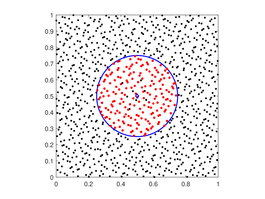
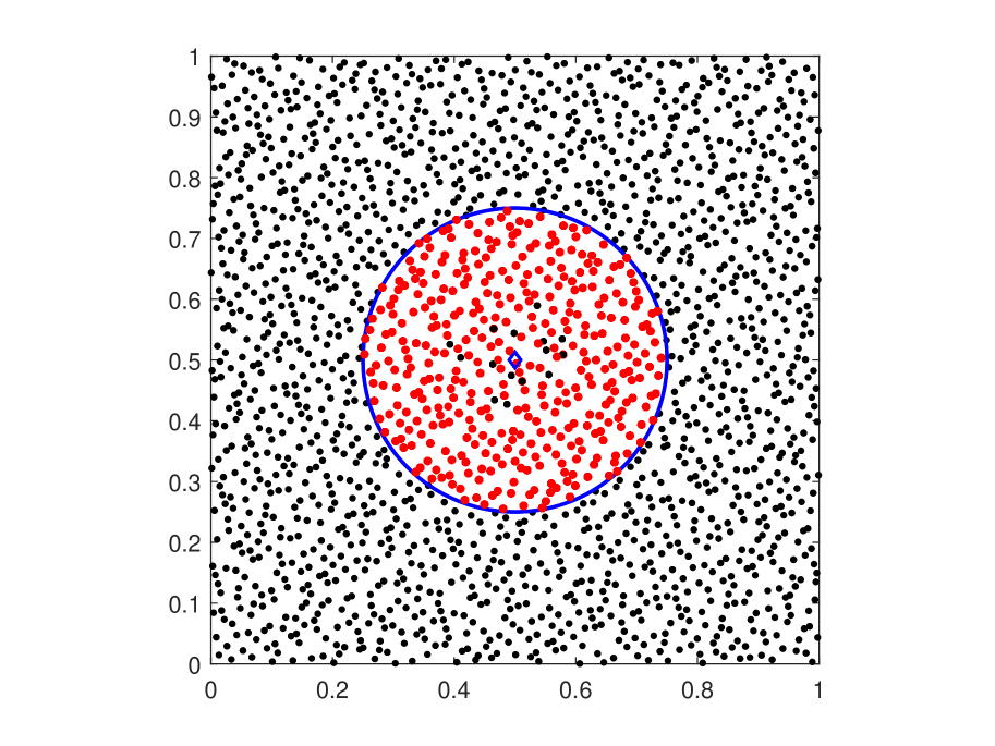
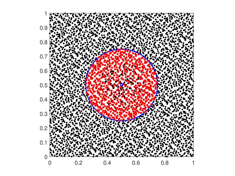
Figure 1. The interpolation points (in red) in the ball of radius $r=1/4$ centered at $(0.5,0.5)$ selected from $1000$ (left), $2000$ (center) and $4000$ (right) Halton points at degrees $d=17,25,35$, respectively, corresponding to minimal errors in Figure 2.

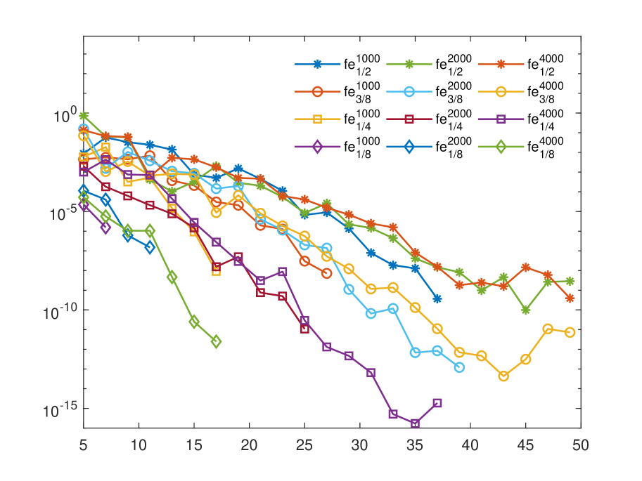
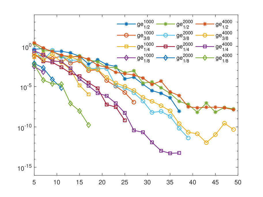
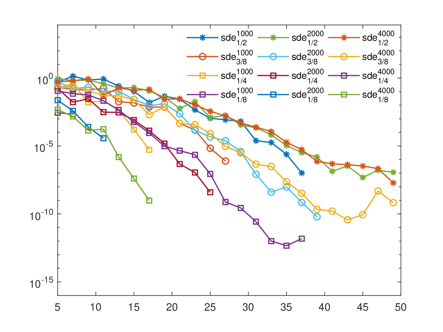
Figure 2. Relative errors (3.1)-(3.3) for function $f_{1}$ by using the subsets of $1000$, $2000$ and $4000$ Halton points intersecting $B_{r}\left(\overline{\mathbf{x}}\right)$, where $\overline{\mathbf{x}}=\left(0.5,0.5\right)$ and $r=\frac{1}{2},\frac{3}{8},\frac{1}{4},\frac{1}{8}$ on a sequence of degrees. Note that shorter sequences (missing marks) are due to a lack of points for interpolation of higher degree.

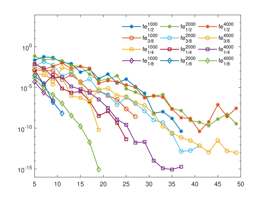
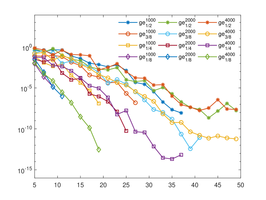
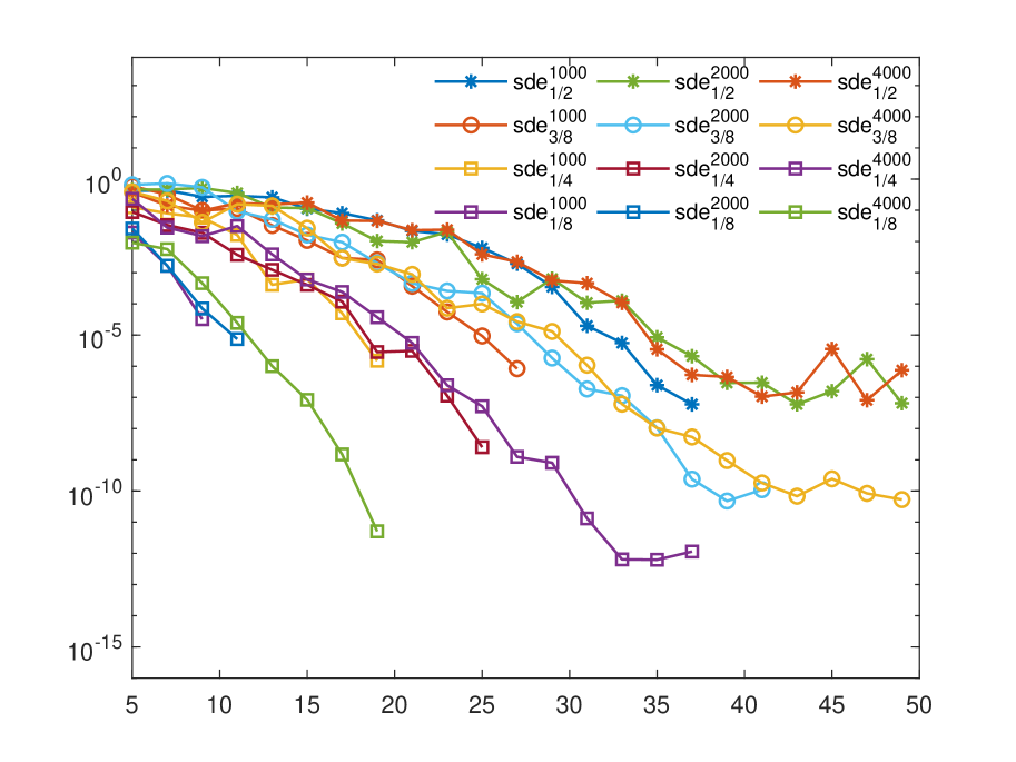
Figure 3. As in Figure 2 starting from uniform random points.

In the second experiment, we start from $2000$ Halton points for the test function $f_{2}$, again with $\overline{\mathbf{x}}=\left(0.5,0.5\right)$. The numerical results are displayed in Figure 4.

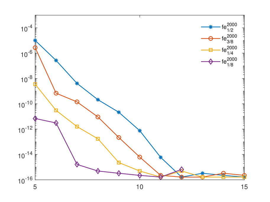
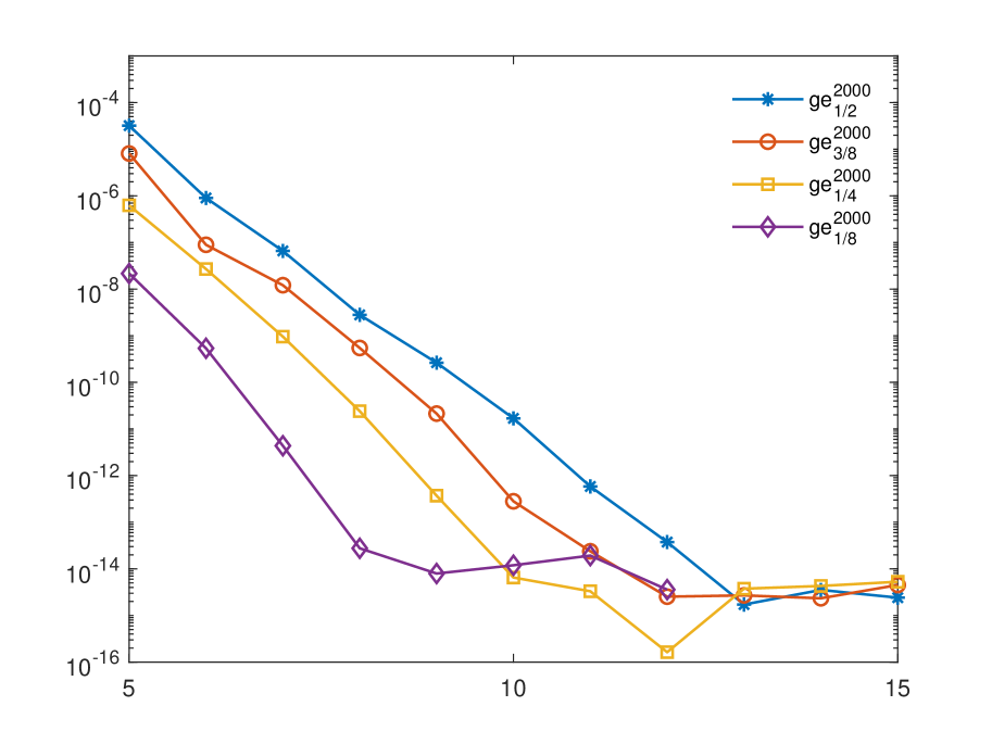
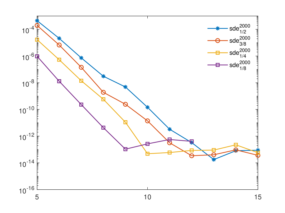
Figure 4. Relative errors (3.1)-(3.3) for function $f_{2}$ using $2000$ Halton points with $\overline{\mathbf{x}}=\left(0.5,0.5\right)$.

In the third experiment, for the test function $f_{3}$, we start from $4000$ Halton points choosing $\overline{\mathbf{x}}$ at the center, then close to the right side and finally close to the north-east corner (see Figures 5-6). The numerical results are displayed in Figures 7, 8 and 10. We repeat the same experiments choosing $\overline{\mathbf{x}}$ on the right side and at the north-east corner and we report the results in Figures 9 and 11.

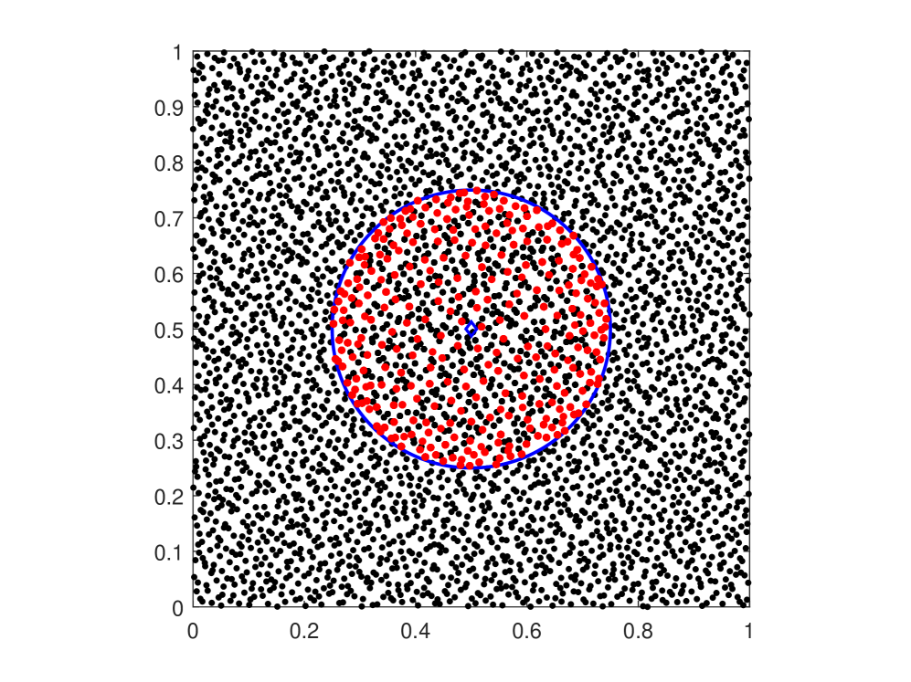
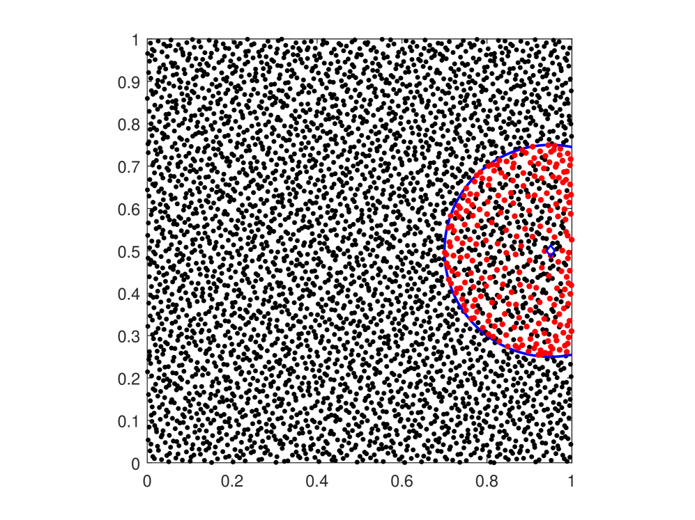
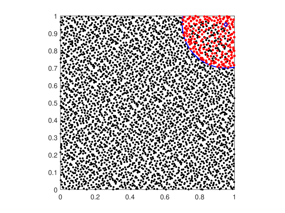
Figure 5. The interpolation points (in red) in the ball of radius $r=1/4$ centered at $\overline{\mathbf{x}}=(0.5,0.5)$ (left), $(0.95,0.5)$ (center), $(0.95,0.95)$ (right) selected from $4000$ Halton points for $d=20$.

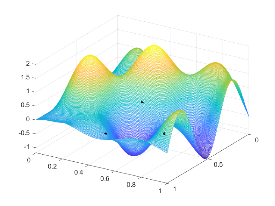
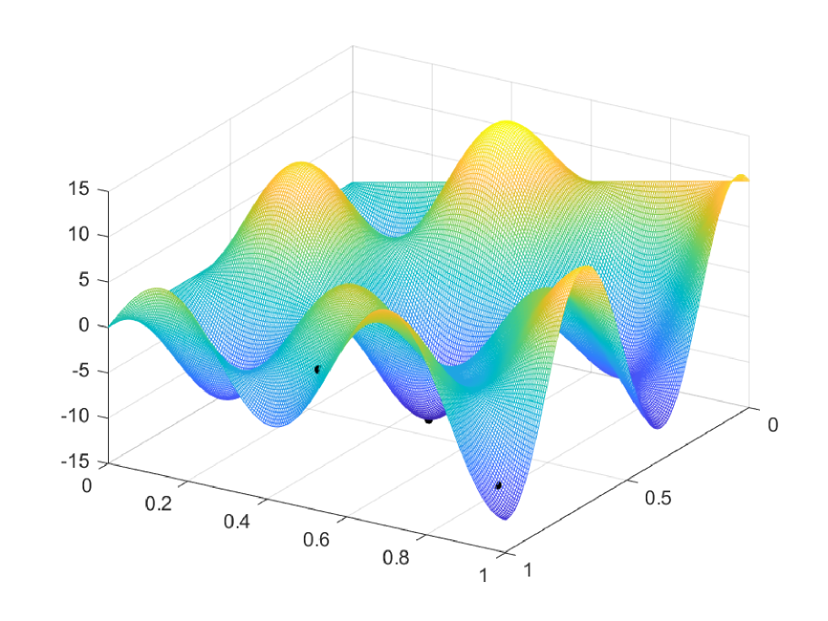
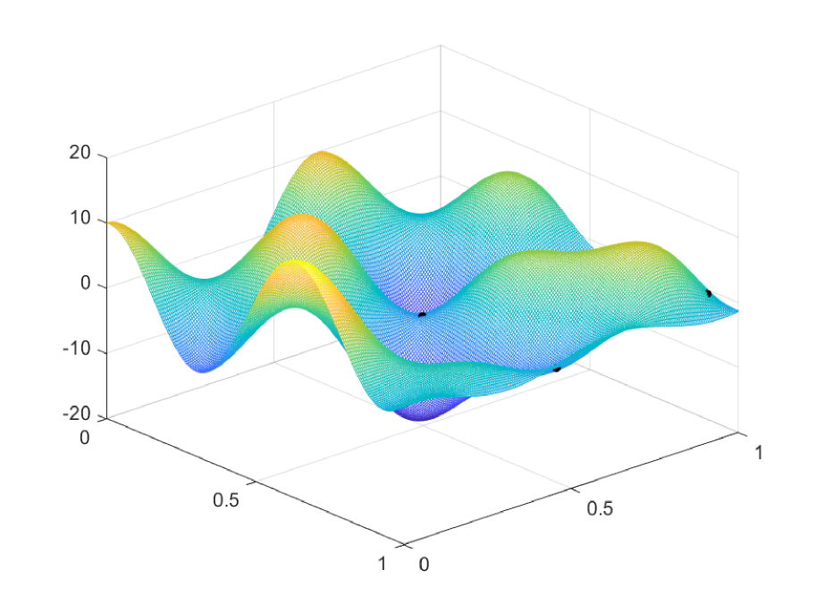
Figure 6. Plot of the function $f_{3}$ (left), $\frac{\partial f_{3}}{\partial x}$ (center), $\frac{\partial f_{3}}{\partial y}$ (right); the surface points corresponding to $\overline{\mathbf{x}}=(0.5,0.5)$, $(0.95,0.5)$, and $(0.95,0.95)$ are displayed with black circles.

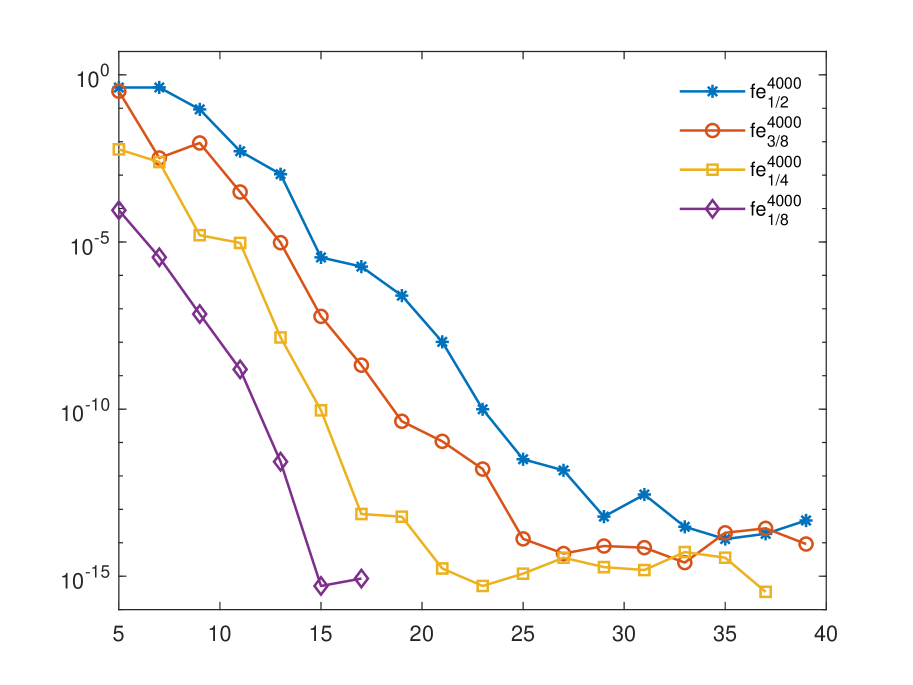
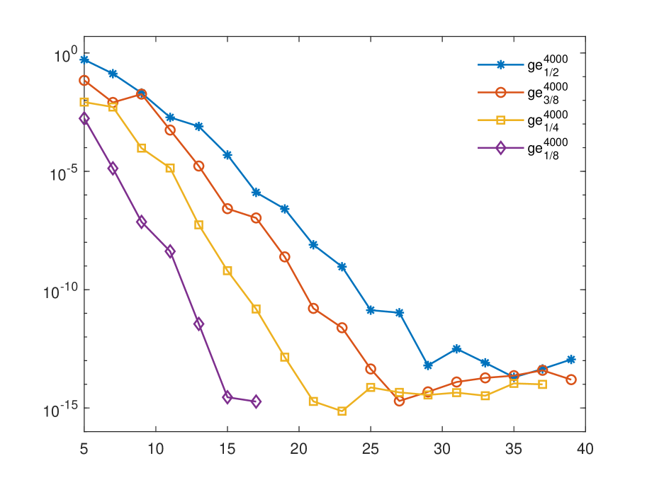
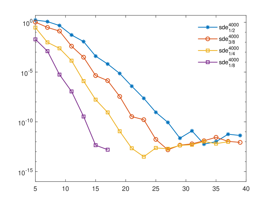
Figure 7. Relative errors (3.1)-(3.3) for function $f_{3}$ by using $4000$ Halton points with $\overline{\mathbf{x}}=(0.5,0.5)$.

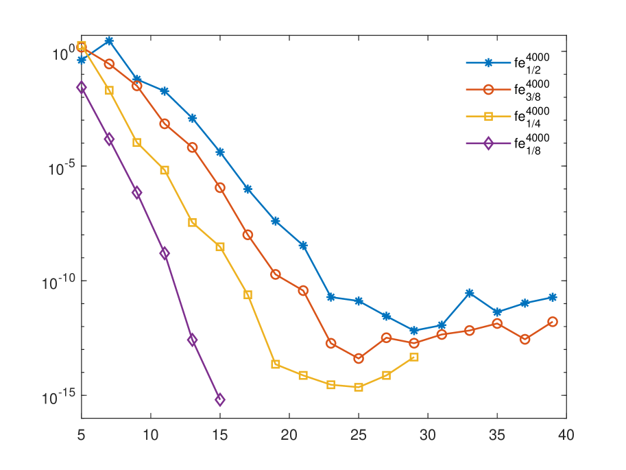
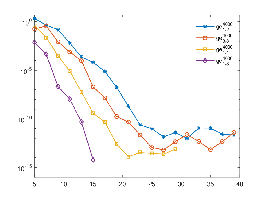
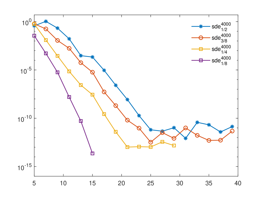
Figure 8. Relative errors (3.1)-(3.3) for function $f_{3}$ by using $4000$ Halton points with $\overline{\mathbf{x}}=(0.95,0.5)$.

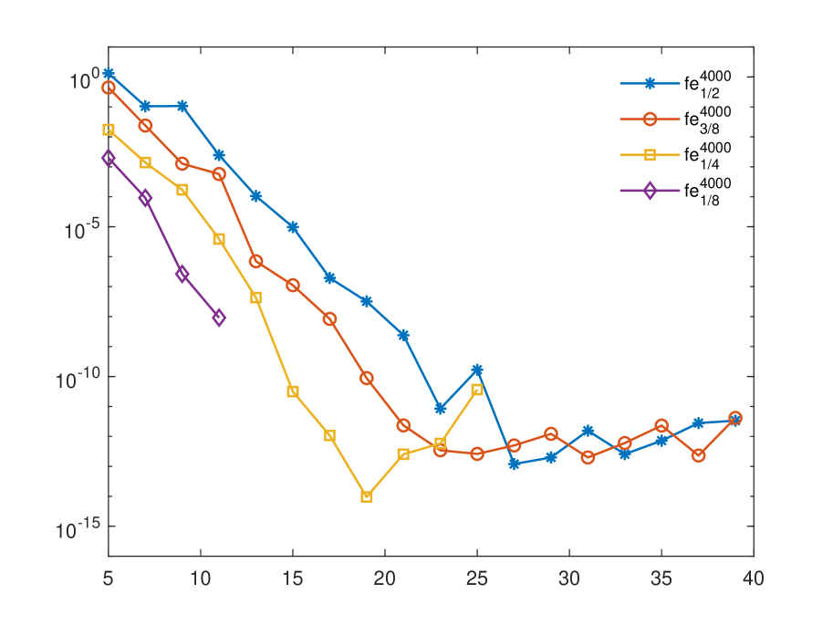
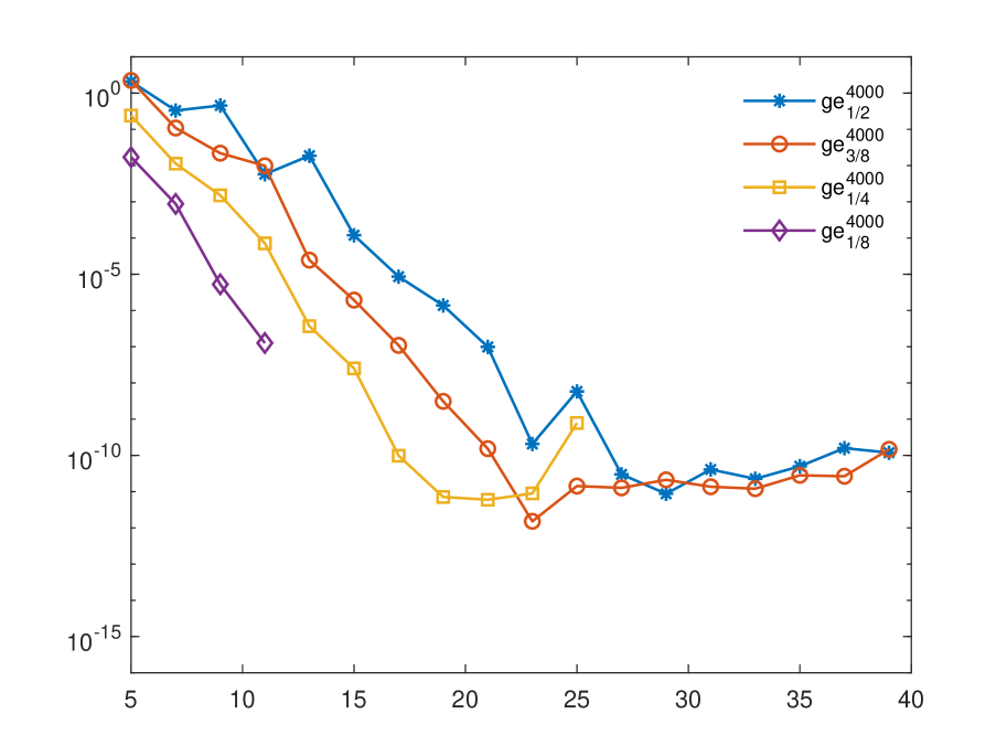
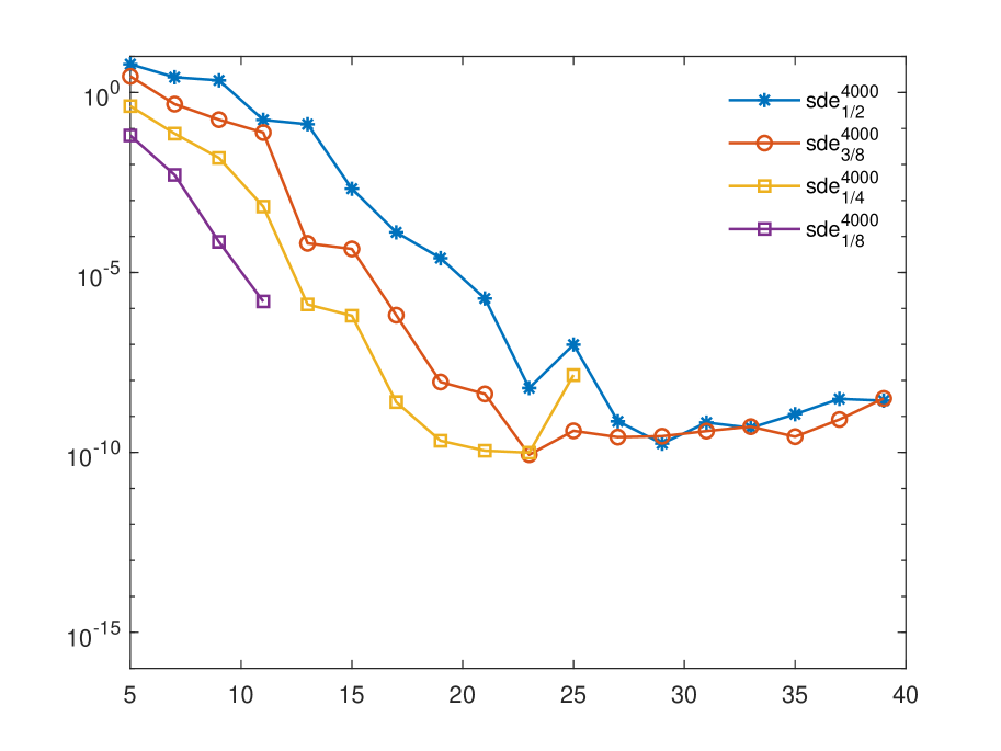
Figure 9. Relative errors (3.1)-(3.3) for function $f_{3}$ by using $4000$ Halton points with $\overline{\mathbf{x}}=(1,0.5)$.

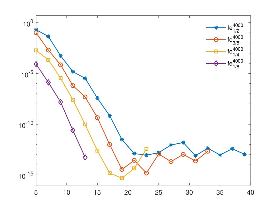
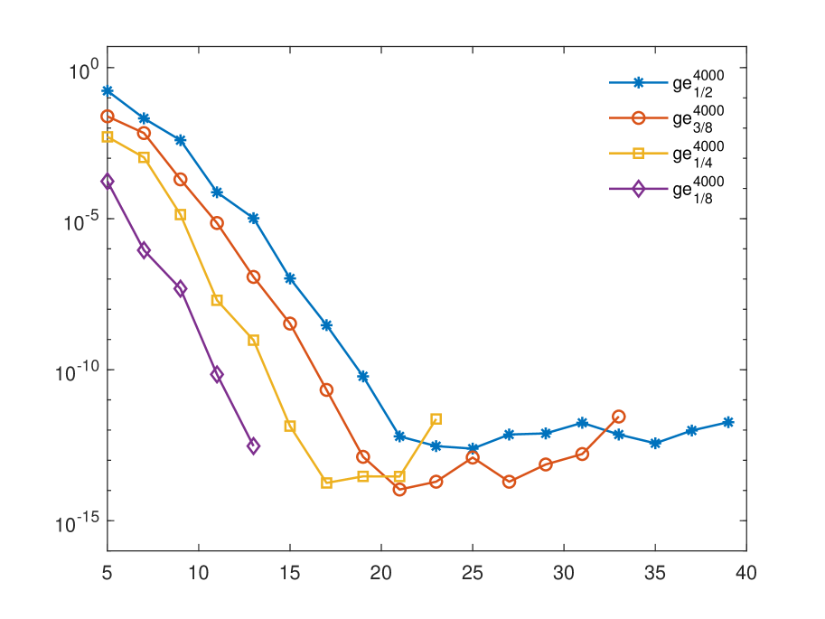
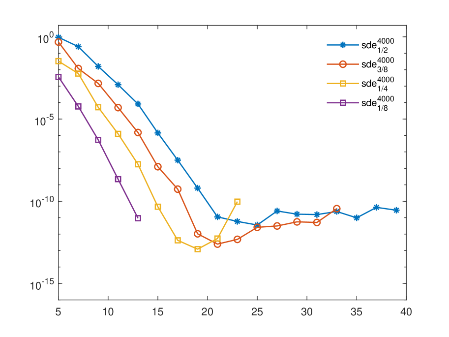
Figure 10. Relative errors (3.1)-(3.3) for function $f_{3}$ by using $4000$ Halton points with $\overline{\mathbf{x}}=(0.95,0.95)$.

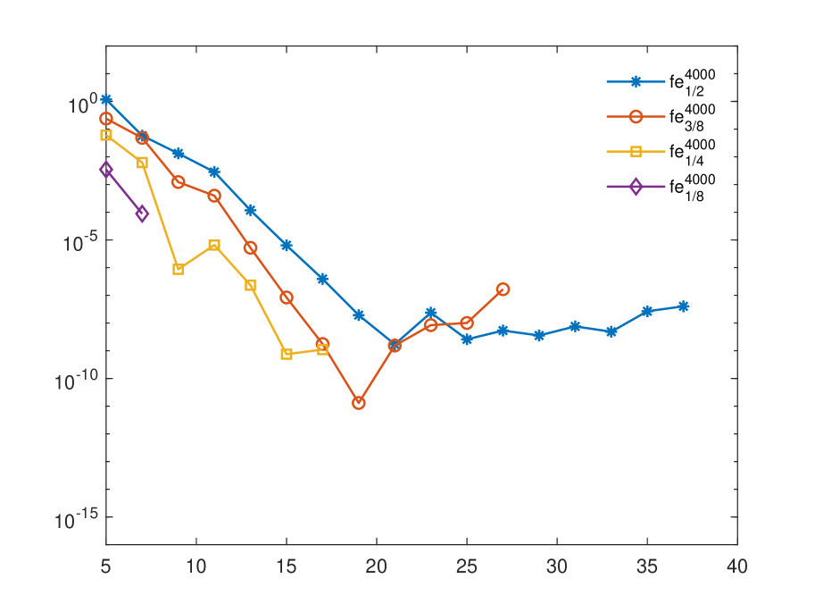
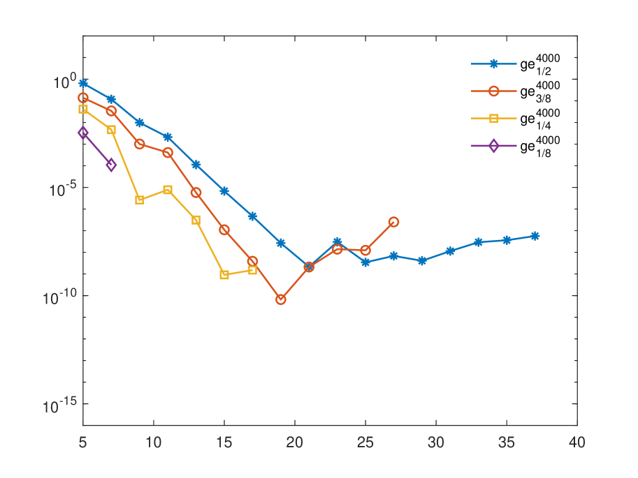
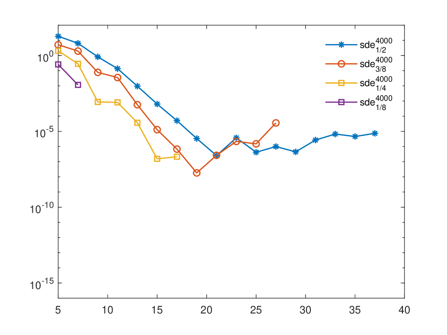
Figure 11. Relative errors (3.1)-(3.3) for function $f_{3}$ by using $4000$ Halton points with $\overline{\mathbf{x}}=(1,1)$.

In the last experiment, for each test function $f_{k}$, $k=1,2,3$, we include a random noise in the $m$ function values, namely

(3.5) $$\tilde{y}=y+U(-\varepsilon,\varepsilon),$$

where $U(-\varepsilon,\varepsilon)$ denotes the multivariate uniform distribution in $[-\varepsilon,\varepsilon]^{m}$. In Figure 12 we display the relative error

(3.6) $$gep=\frac{\left\|\nabla{f}(\overline{\mathbf{x}})-\nabla\widetilde{{p}}(\overline{\mathbf{x}})\right\|_{2}}{\left\|\nabla{f}(\overline{\mathbf{x}})\right\|_{2}}$$

for the gradient at $\overline{\mathbf{x}}=\left(0.5,0.5\right)$, computed using $1000$ Halton points with exact function values (3.2) and perturbed function values (3.6) for $\varepsilon=10^{-6}$. In Figure 13 we display the relative sensitivity in computing the gradient of the interpolating polynomial $p$ under the perturbation of the function values ($\varepsilon=10^{-6}$)

(3.7) $$gs=\frac{\left\|\nabla{p}(\overline{\mathbf{x}})-\nabla\widetilde{{p}}(\overline{\mathbf{x}})\right\|_{2}}{\left\|\nabla{f}(\overline{\mathbf{x}})\right\|_{2}},$$

together with its estimate involving the stability constant of the gradient (2.33)

(3.8) $$gse=\frac{\left\|\left(\varepsilon h^{-1}\sum\limits_{i=1}^{m}\left|a_{(1,0),h}^{i}\right|,\varepsilon h^{-1}\sum\limits_{i=1}^{m}\left|a_{(0,1),h}^{i}\right|\right)\right\|_{2}}{\left\|\nabla{f}(\overline{\mathbf{x}})\right\|_{2}}.$$

Notice that the relative errors $gep$ in Figure 12 and sensitivity $gs$ in Figure 13 are of the same order of magnitude when the errors $ge$ become negligible with respect to $gs$. Moreover, $gse$ turns out to be a slight overestimate of the relative sensitivity $gs$. This fact, as we can see in Table 2 where $\overline{\mathbf{x}}=(0.5,0.5)$, is due to the relative small values of the stability constant that varies slowly while decreasing the radius $r$ or increasing the degree of the interpolating polynomial.

Finally, it is worth stressing that the stability constant (2.33) is a function of $\overline{\mathbf{x}}$ and then it depends on the position of $\overline{\mathbf{x}}$ in the square. More precisely, for a fixed interpolation degree $d$, it slowly varies except for a neighborhood of the boundary where it increases rapidly, expecially near the vertices, as can be observed in Figure 14, where for clarity we restrict the stability constant to lines. On the other hand, it can be noticed that by increasing the degree, the stability constant tends to increase, much more rapidly at the boundary. Such a behavior, that explains the worsening of the accuracy at the boundary (see Figures 8-9) and at the vertex (see Figures 10-11) of the square, can be ascribed to the fact that the stability functions (2.34) increase rapidly near the boundary of the local interpolation domains $B_{h}(\overline{\mathbf{x}})\cap\Omega$. This phenomenon, that resembles the behavior at the boundary of Lebesgue functions of univariate interpolation at equispaced points [16], is worth of further investigation.

			$d=5$	$d=10$	$d=15$	$d=20$	$d=25$
		$r=1/2$	2.31	2.43	6.69	2.41e+1	3.51e+1
	$\left|\nu\right|=0$	$r=3/8$	1.75	4.10	1.11e+1	2.91e+1	3.03e+1
		$r=1/4$	2.14	4.73	7.16	-	-
		$r=1/8$	1.80	-	-	-	-
		$r=1/2$	2.63e+1	7.26e+1	4.53e+2	9.06e+2	7.74e+2
	$\left|\nu\right|=1$	$r=3/8$	2.85e+1	1.64e+2	3.51e+2	6.04e+2	9.55e+2
		$r=1/4$	3.61e+1	1.67e+2	3.84e+2	-	-
		$r=1/8$	1.27e+2	-	-	-	-
		$r=1/2$	9.94e+1	1.41e+3	3.30e+3	1.82e+4	3.05e+4
	$\left|\nu\right|=2$	$r=3/8$	1.72e+2	2.80e+3	7.94e+3	3.61e+4	5.15e+4
		$r=1/4$	4.02e+2	4.54e+3	2.02e+4	-	-
		$r=1/8$	1.73e+3	-	-	-	-

Table 2. Numerical comparison among the mean value of the stability constant (2.33) with $\left|\nu\right|\leq 2$, for interpolation at a sequence of degrees $d$ on Discrete Leja points extracted from the subset of $1000$ Halton points in $[0,1]^{2}$ contained in the ball $B_{r}(\overline{\mathbf{x}})$ centered at $\overline{\mathbf{x}}=(0.5,0.5)$.

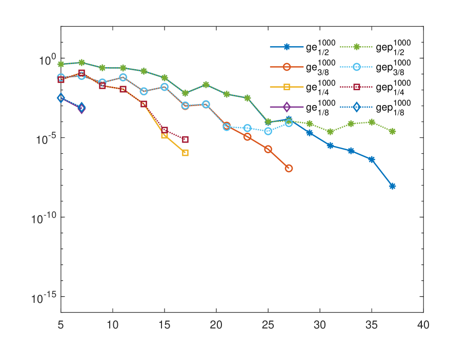
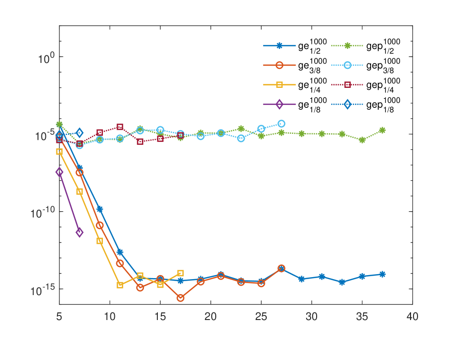
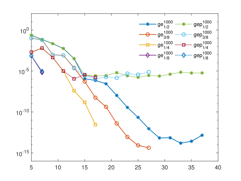
Figure 12. Relative error (3.2) for the gradient computed with exact ($ge$) and perturbed ($gep$) function values (3.5) for the functions $f_{1}$ (left), $f_{2}$ (center) and $f_{3}$ (right) by using $1000$ Halton points with $\overline{\mathbf{x}}=(0.5,0.5)$.

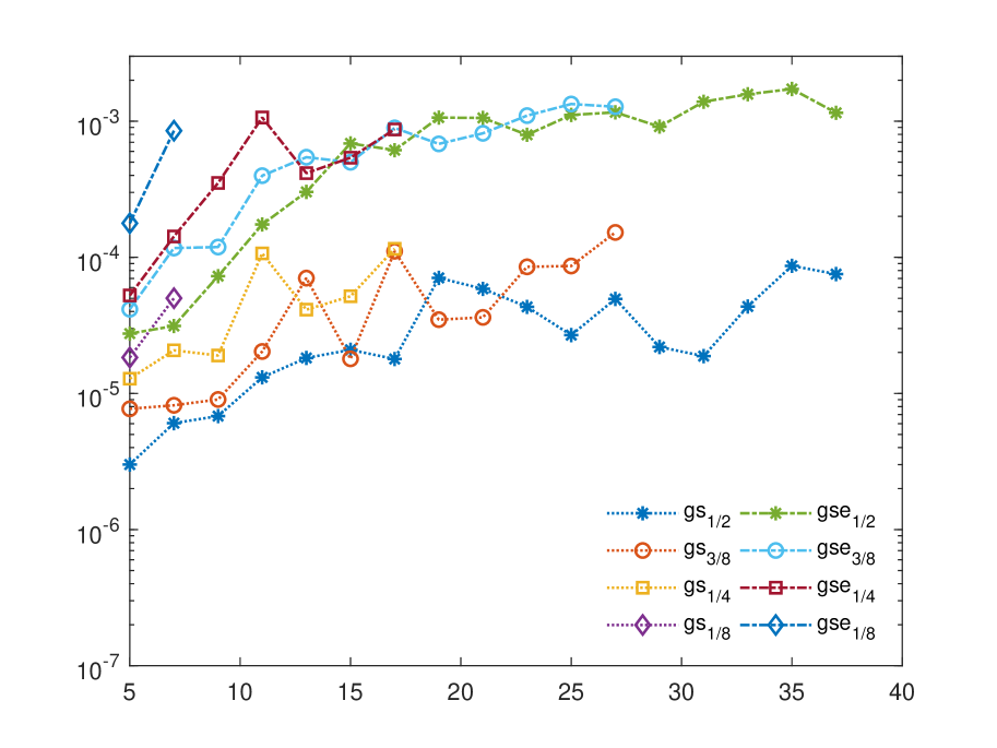
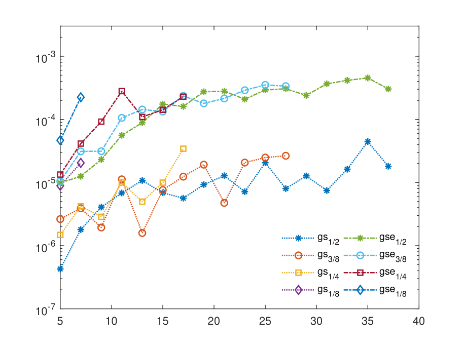
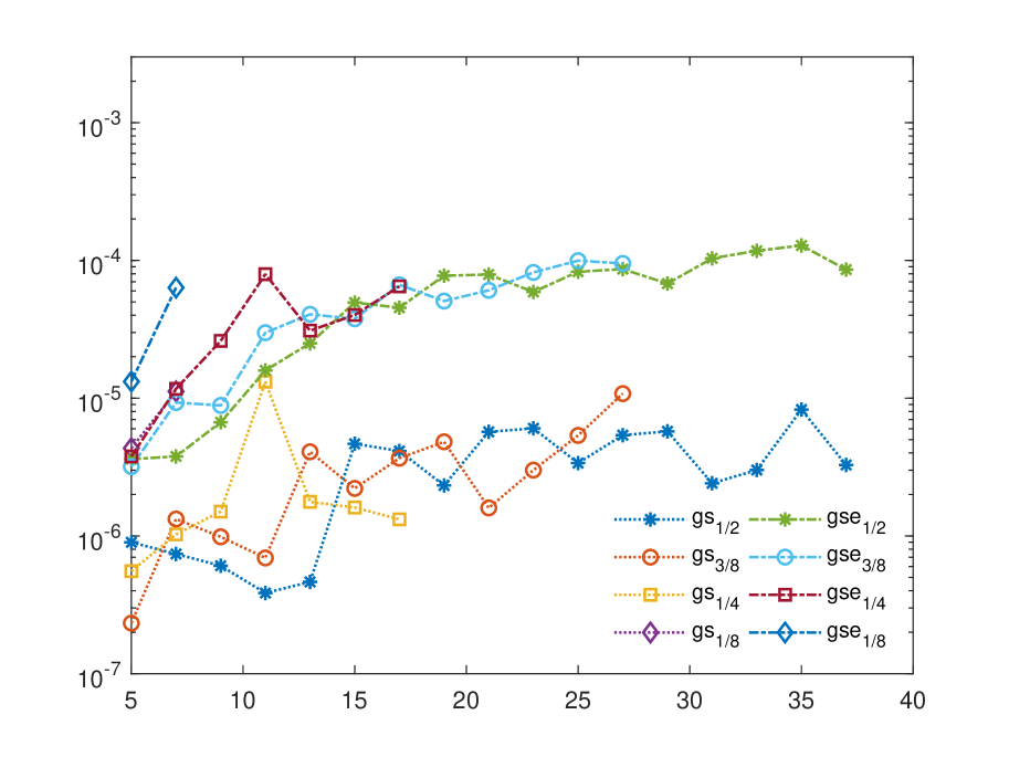
Figure 13. Relative sensitivity (3.7) for the gradient of $p$ computed with perturbed function values ($gs$) and its estimate (3.8) involving the stability constant of the gradient ($gse$) for the functions $f_{1}$ (left), $f_{2}$ (center) and $f_{3}$ (right) by using $1000$ Halton points with $\overline{\mathbf{x}}=(0.5,0.5)$.

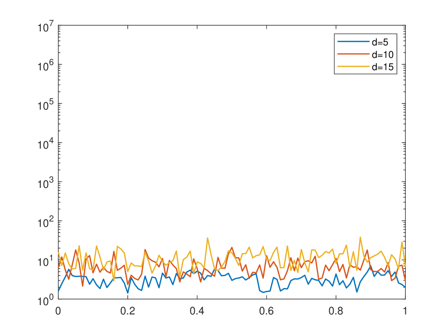
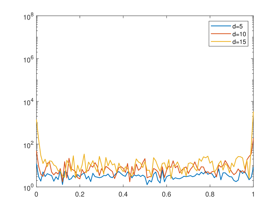
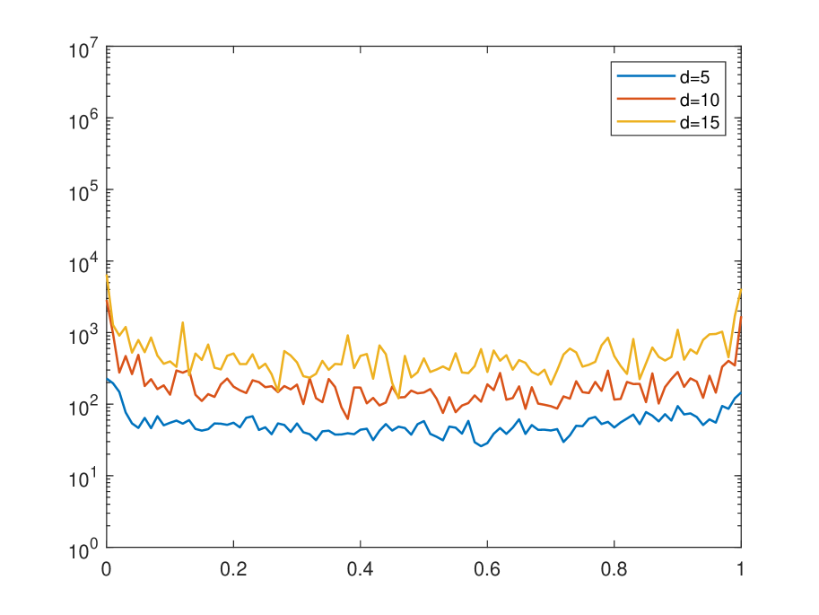
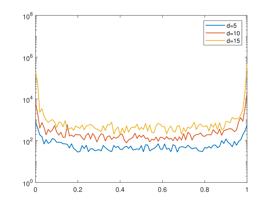
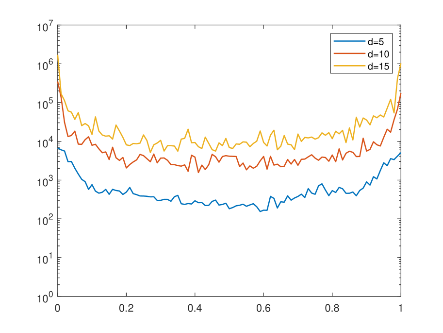
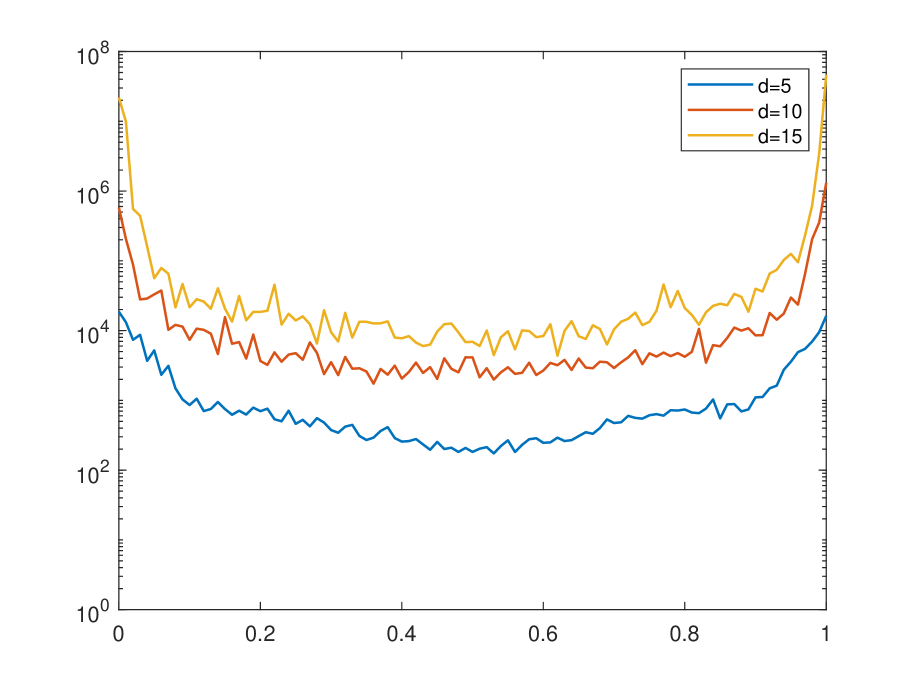
Figure 14. The stability constant (2.33), for degrees $d=5,10,15$ and $|\nu|=0$ (left), $|\nu|=1$ (center) and $|\nu|=2$ (right) computed by using $4000$ Halton points with $r=1/2$ and $\overline{\mathbf{x}}$ being $101$ equispaced points on the horizontal line $y=0.5$ (top) and on the diagonal $y=x$ (bottom).

References

[1]
John A Belward, Ian W Turner, and Miloš Ilić.
On derivative estimation and the solution of least squares problems.
Journal of Computational and Applied Mathematics,
222(2):511–523, 2008.
[2]
Len Bos, Stefano De Marchi, Alvise Sommariva, and Marco Vianello.
Computing multivariate Fekete and Leja points by numerical linear
algebra.
SIAM Journal on Numerical Analysis, 48(5):1984–1999, 2010.
[3]
Roberto Cavoretto, Alessandra De Rossi, Francesco Dell’Accio, and Filomena
Di Tommaso.
Fast computation of triangular Shepard interpolants.
Journal of Computational and Applied Mathematics, 354:457–470,
2019.
[4]
Roberto Cavoretto, Alessandra De Rossi, Francesco Dell’Accio, and Filomena
Di Tommaso.
An efficient trivariate algorithm for tetrahedral Shepard
interpolation.
Journal of Scientific Computing, 82(3):1–15, 2020.
[5]
Elliott Ward Cheney and William Allan Light.
A course in approximation theory, volume 101.
American Mathematical Soc., 2009.
[6]
Oleg Davydov and Robert Schaback.
Error bounds for kernel-based numerical differentiation.
Numerische Mathematik, 132(2):243–269, 2016.
[7]
Oleg Davydov and Robert Schaback.
Minimal numerical differentiation formulas.
Numerische Mathematik, 140(3):555–592, 2018.
[8]
Francesco Dell’Accio and Filomena Di Tommaso.
Rate of convergence of multinode Shepard operators.
Dolomites Research Notes on Approximation, 12(1), 2019.
[9]
Francesco Dell’Accio and Filomena Di Tommaso.
On the hexagonal Shepard method.
Applied Numerical Mathematics, 150:51–64, 2020.
[10]
Francesco Dell’Accio, Filomena Di Tommaso, and Kai Hormann.
On the approximation order of triangular Shepard interpolation.
IMA Journal of Numerical Analysis, 36(1):359–379, 2016.
[11]
Francesco Dell’Accio, Filomena Di Tommaso, and Najoua Siar.
On the numerical computation of bivariate Lagrange polynomials.
Applied Mathematics Letters, page 106845, 2020.
[12]
Reinhard Farwig.
Rate of convergence of Shepard’s global interpolation formula.
Mathematics of Computation, 46(174):577–590, 1986.
[13]
Ladislav Kocis and William J Whiten.
Computational investigations of low-discrepancy sequences.
ACM Transactions on Mathematical Software (TOMS),
23(2):266–294, 1997.
[14]
Leevan Ling and Qi Ye.
On meshfree numerical differentiation.
Analysis and Applications, 16(05):717–739, 2018.
[15]
Robert J Renka and Ron Brown.
Algorithm 792: accuracy test of ACM algorithms for interpolation of
scattered data in the plane.
ACM Transactions on Mathematical Software (TOMS), 25(1):78–94,
1999.
[16]
Lloyd N Trefethen.
Approximation Theory and Approximation Practice,
Extended Edition.
SIAM, 2019.
[17]
Shayne Waldron.
Multipoint Taylor formulæ.
Numerische Mathematik, 80(3):461–494, 1998.
[18]
Don R Wilhelmsen.
A Markov inequality in several dimensions.
Journal of Approximation Theory, 11(3):216–220, 1974.