From parcel to continental scale - A first European crop type map based on Sentinel-1 and LUCAS Copernicus in-situ observations

Abstract

Detailed parcel-level crop type mapping for the whole European Union (EU) is necessary for the evaluation of agricultural policies in the European Union (EU). The Copernicus program, and Sentinel-1 (S1) in particular, offers the opportunity to monitor agricultural land at a continental scale and in a timely manner. However, so far the potential of S1 has not been explored at such a scale. Capitalizing on the unique LUCAS 2018 Copernicus module, we present the first continental crop type map at 10-m spatial resolution for the European Union (EU) based on S1A and S1B Synthetic Aperture Radar observations for the year 2018. We combined time series of 10-day average VV and VH S1 sigma backscattering coefficients from January to end of July with crop type information from the LUCAS 2018 survey. Random forest classification algorithms are tuned for two strata (a northern continental and a southern Mediterranean) and a two-phase classification procedure that distinguishes three main vegetation classes in the first phase and 19 different crop types (or crop type groups) in the second phase. Non-vegetation land cover classes are masked out using auxiliary information and areas above 1,000 m and with a steep slope are discarded. We assess the accuracy of this EU crop map with three approaches. First, the accuracy is assessed with independent LUCAS core in-situ observations across the EU. Second, an accuracy assessment is done specifically for main crop types from farmers declarations (GSAA, geospatial aid application) from 6 EU member countries or regions totaling $>$3M parcels and 8.21 Mha. Finally, for the main crops, the crop areas derived by classification are compared to the subnational (NUTS 2) area statistics reported by Eurostat. The overall accuracy for the map is reported as 80.3% when grouping main crop classes and 76% when considering all 19 crop type classes separately. Highest accuracies are obtained for rape and turnip rape with user and produced accuracies higher than 96%. Crop specific and phenology driven features determine the classification accuracy throughout the growing season. We highlight confusion between common wheat and barley, mainly due to the crop structure and phenology. A confusion between sugar beet and maize is also observed and likely due to the early time constraint we imposed for the classification production, i.e. end of July. The correlation between the remotely sensed estimated and Eurostat reported crop area ranges from 0.93 (potatoes) to 0.99 (rape and turnip rape). Finally, we discuss how the framework presented here can underpin the operational delivery of in-season high-resolution based crop mapping for the EU.

1 Introduction

The European Union (EU) is the largest global exporter of agri-food products, with exports reaching €138 billion in 2018 [European Commission, 2019]. Farmlands are an important feature of the EU landscape with about 42% of the EU’s land area dedicated to agriculture. At the same time, the EU’s Common Agricultural Policy (CAP) makes up about 37% of the European Commission’s (EC) budget (€58.8 billion in 2018). Besides underpinning resilient food production, the CAP could contribute to mitigate climate change, improve the sustainable management of natural resources, and preserve biodiversity and landscapes. This is in line with the European Green Deal, and the Farm to Fork and Biodiversity strategies. Updated EU-wide information on crop types is essential to evaluate the implementation of these agricultural policies. The EU’s Copernicus space programme and technological advances provide the opportunity to transform the ways in which we monitor crops, agricultural practices, as well as CAP expenditure. Moreover, in order to forecast crop yields and production in the EU, independent and timely information is needed to support decisions regarding agricultural markets of cereals and other crops. [van der Velde et al., 2019].

The Copernicus Sentinel-1 (S1) mission adds unique features to our global Earth Observation (EO) capacity. The frequency of observations is guaranteed by the S1A and S1B polar-orbiting satellites acquiring all-weather (not affected by atmospheric conditions) C-band Synthetic Aperture Radar imagery. Here we exploit this capability for continental scale agricultural monitoring at 10-m resolution. The use of microwave detection for large scale crop type mapping remains underexploited, opposed to applications using optical imagery, e.g. Belgiu & Csillik [2018], Immitzer et al. [2016] and Defourny et al. [2019]. Recently, the use of high performance cloud computing on platforms such as Google Earth Engine (GEE, Gorelick et al. [2017]) has been demonstrated for detailed continental scale crop-type mapping. Massey et al. [2018] and Teluguntla et al. [2018] used large collections of 30-m optical LANDSAT imagery to respectively classify crops over North America, and over China and Australia.

Besides the recent developments in computational capacity to handle such large data streams and related algorithms, complementary in-situ observations remain essential for training and validation purposes. In the EU, continental in-situ data collection is organised through the Land Use/Cover Area frame Survey (LUCAS) [Gallego & Delincé, 2010, Eurostat, 2018a]. In 2018, the Copernicus module - a survey protocol specifically tailored to EO - was introduced [d’Andrimont et al., 2021], providing a unique set of polygons with homogeneous land cover (covering up to 0.52 ha) with land cover as well as crop specific information. Another source of in-situ data is the parcel-level crop declarations by farmers in the context of the CAP, which are increasingly publicly available. Here, we bring these elements together to create the first validated crop type map for the EU at 10-m resolution. After reviewing the pertinent literature in detail, we present the specific objectives of this study.

1.1 Crop mapping with Sentinel-1

The SAR S1 constellation provides minimum consistent 6-day revisits over the EU since 2016. The negligible dependence of microwave backscatter on atmospheric conditions provides consistent calibrated time series that are particularly well-suited for automated processing and machine learning. The sensitivity of microwave backscattering to crop canopy structure [Dobson & Ulaby, 1981, Ulaby et al., 1981, Veloso et al., 2017, d’Andrimont et al., 2020a, Meroni et al., 2021], along with its sensitivity to soil surface structure and moisture content [Dobson & Ulaby, 1981] makes it an ideal data source for crop mapping. One of the overall principles in electromagnetic scattering models of crop canopies is that (back)scattering depends on leaf size and shape, relative to the microwave wavelength, their orientation in space, relative to the polarization plane of the microwaves, and the water content of those leafs. Leaf geometry and orientation determines, to a large extent, the preferential (back)scattering direction. This explains the large differences in vertically structured crop canopies (e.g. cereals) versus broad-leaf crops (e.g. sugarbeet, potatoes). It also implies that backscattering changes are expected for phenological stages of the crop that cause structural change in the canopy (ear formation in cereals, fruit formation after flowering). The leaf water content relates to the effective dielectric properties of the canopy, which determines (back)scattering intensity. Vigorous, well-watered crop canopies are more effective scatterers than stressed or senescent crops, which scattering behavior may be modulated by simultaneous change in leaf orientation. Scattering of bare soil is primarily dependent on surface roughness and soil moisture content, which has parallels to canopy scattering because the relative size and orientation of the surface structure is important, as well as row direction of the soil cultivation and soil water content, which determines scattering effectivity via the dielectric properties. It follows that scattering of partially vegetated soil, e.g., at the crop emergence stage, is related to the ensemble of canopy and soil scattering effects and that variation over time is related to the relative contributions of each component. Polarization of the microwaves determines the (Fresnel) reflection coefficients of the canopy and soil material.

Synthetic Aperture Radar (SAR) has been used as a data source for crop type mapping in different studies [McNairn & Brisco, 2004, Kenduiywo et al., 2018, Clauss et al., 2018], as well as in synergistic combination with optical data [Van Tricht et al., 2018, Gao et al., 2018, Kussul et al., 2018, Orynbaikyzy et al., 2020, Chakhar et al., 2021]. Despite all the advantages of SAR, relatively few studies have focused on crop mapping based on S1 only. Kussul et al. [2017] and Van Tricht et al. [2018] derived a crop type map from a combination of S1 with optical data over Ukraine and Belgium respectively. Other local studies over the Chinese Fuyu City [Wei et al., 2019] and the French Camargue region [Ndikumana et al., 2018], demonstrate the potential of using S1 for crop type mapping. The consistent availability of S1 observations is particularly relevant in machine learning contexts. Such consistency is difficult to achieve with optical Sentinel-2 data, due to unpredictable cloud cover gaps in a multi-annual monitoring setting. Early results with the use of S1 time series in a deep neural network approach [Lemoine et al., 2019] demonstrated this successfully in a national EU crop mapping context.

1.2 In-situ data in the European Union

There is growing interest in using LUCAS in-situ data for land cover and land use research [Pflugmacher et al., 2019, Weigand et al., 2020]. However, until the recent harmonization of the five past LUCAS surveys by d’Andrimont et al. [2020b], use of different LUCAS survey data remained difficult. In addition, the LUCAS protocol was designed for EU-wide standardized reporting of land cover and land use area statistics and not for Earth Observation (EO) applications.

Past remote sensing studies that incorporated LUCAS core data have been limited to statistical area estimates [Gallego & Delincé, 2010]. The LUCAS sampling frame was used to assess availability of crowd-sourced pictures potentially relevant for agriculture across the EU [d’Andrimont et al., 2018b]. Little experience exists in using LUCAS data for large scale land cover generation processes, especially on the usability of the LUCAS data set as training data base for supervised classification approaches [Mack et al., 2017]. The 2015 survey was used in several land cover and land use mapping exercises. Close et al. [2018] provided a Sentinel-2 LUCAS-based classification over southern Belgium in the context of Land Use, Land-Use Change, and Forestry (LULUCF) monitoring. Pflugmacher et al. [2019] demonstrated the potential of using LUCAS survey 2015 to map pan-European land cover (13 classes) with Landsat data. Weigand et al. [2020] showed the suitability of the LUCAS 2015 survey as reference information for high resolution land cover mapping using Sentinel-2 imagery at the scale of Germany (7 classes).

In 2018, a new LUCAS module (the Copernicus module) specifically tailored to EO was introduced, see d’Andrimont et al. [2021]. A specific protocol was designed to collect in-situ information with specific characteristics fitting EO processing requirements. As a result, a total of 58,428 polygons are provided with a level-3 land cover (66 specific classes including crop type) and land use (38 classes) information. This represent a unique set of data opening the possibility for applications with higher thematic detail as compared to previous LUCAS surveys, such as crop type mapping.

1.3 Objectives

The overall aim of this study is to assess the potential of combining the LUCAS Copernicus module with S1 data to generate an EU-wide crop type map at 10-m spatial resolution for crops in the year 2018. Beyond the production of the map, this study aims to set a benchmark for continental crop type mapping at 10-m spatial resolution. More specifically, we address the following research objectives:

• To highlight the untapped potential of the LUCAS Copernicus survey as training data for land monitoring applications in general and crop type mapping in particular;

• To demonstrate the value of S1 data for continental crop type map production;

• To evaluate the effectiveness of various S1 indices and time periods for the discrimination of specific crop types;

• To benchmark accuracies against independent LUCAS core point data and EU farmers’ declarations at parcel level;

• To determine the crop specific evolution of mapping accuracy throughout the growing season relevant for prospective operational tasks;

• To assess crop surface areas derived from the 10-m crop type map against reported EU statistics at subnational level.

2 Materials and Methods

The study area is the EU-28 as in 2018, covering $4,469,169$ km² (Fig. 2). A 10-km buffer was applied around the EU-28 to avoid mapping issues at the border.

Fig. 1 provides a flow chart illustrating the general approach and specific methodological steps of the study. First, the input data is detailed: S1 in section 2.1 and in-situ data in Section 2.2. Then, Section 2.3 defines the legend used for the study. While Section 2.4 sets out how the features and the parameters for the crop classification models are selected, Section 2.5 describes how the classification is applied at the continental scale. Finally, Section 2.6 presents the three accuracy assessment approaches.

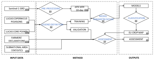
Fig. 1: General overview (references to section number are highlighted in grey).

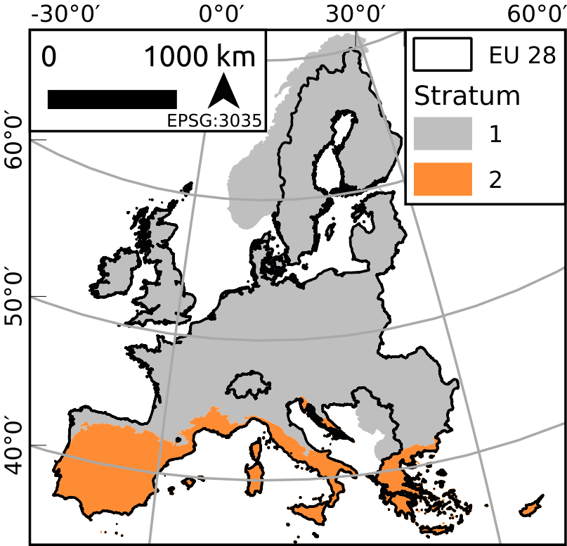
Fig. 2: The study area is the European Union 28 (EU-28). The study area is divided in 2 strata based on a combination of biomes from Dinerstein et al. [2017] as described in Section 2.4.3.

2.1 Sentinel-1 data

The S1 C-band operates at a central frequency of 5.404 Ghz in the microwave portion of the electromagnetic spectrum which corresponds to a wavelength of 5.55 cm. S1 acquisitions over the European land mass are in the so-called interferometric wave (IW) mode, which registers the backscattering of a vertically transmitted microwave signal in a vertical and horizontal receiver, creating a VV and VH polarized band, respectively.

Over Europe, S1 acquires data both in descending and ascending orbits, as it does not rely on solar illumination (as opposed to optical sensors). This leads to a doubling of the revisit cycle, though from two distinct sensor viewing configurations due to different azimuth and look directions. Furthermore, the S1 swath width is designed to guarantee gap free coverage at the equator. At higher latitudes, this design leads to considerable overlap between adjacent orbits, and an effective higher revisit, more than daily at latitude above 55 degrees North.

2.1.1 Geocoded backscattering coefficients

Application ready S1 data are accessed on the GEE platform. On GEE, S1 data are processed from the GRD Level-1 product with the S1 Toolbox to remove thermal noise and to create geocoded and radiometrically calibrated backscattering coefficients ($\sigma^{0}$) at 10-m pixel spacing.

Due to the side-looking nature of the SAR sensor, the incidence angle varies over the swath in the range direction, for S1 IW mode between 25-40 degrees. Normalization of the incidence effect is normally desired, and simple corrections can be applied to convert $\sigma^{0}$ to $\gamma^{0}$. A more robust approach would be to apply a correction that takes the local terrain height variation into account, known as terrain flattening (Small [2011]), which can also partially compensate for the look angle differences in ascending and descending orbit acquisitions. However, terrain flattening is not applied in the GEE processing workflow and our analysis is thus based on $\sigma^{0}$ as most of the crops are typically on flat areas and the steep slopes are masked out as described in Section 2.5.

To be ingested in the machine learning classification algorithm, a spatially and temporally consistent time series needs to be derived from the S1 VV and VH $\sigma^{0}$ scenes. In addition, the backscattering coefficient ratio VH/VV (cross polarization ratio, CR) is computed from the VV and VH scenes. Several studies highlighted the advantages of the CR for mapping and monitoring of crops (Veloso et al. [2017], Meroni et al. [2021]). We proceeded as follows to generate the required archive:

1. Edge masking. The edge of each scene should be masked before the compositing. This is done by masking groups of neighboring pixels with values lower than -25 dB in the VV polarization (as described in d’Andrimont et al. [2018a]).

2. Averaging over a 10-day period. $\sigma^{0}$ values are then averaged over subsequent time periods of 10 days for each pixel and for all ascending and descending acquisitions available in that period, separately for the VV and VH polarizations. The averaged $\sigma^{0}$ value is converted to decibels (dB).

3. Computing the cross polarization ratio. The CR is computed for each scene and averaged to the same 10-days periods.

In this way, we generate a regularly timed, gridded, equal sized set of temporal features for VV, VH and CR to use as input for the subsequent machine learning runs (n = 36 10-day composites over the period 2018-01-01 to 2018-12-31), independent of the number of actual S1 acquisitions in the 10-day period. The S1 data were processed in GEE and then downloaded.

2.2 LUCAS 2018 in-situ data

This section describes the LUCAS 2018 survey data that were used for training the classification models and assessing the accuracy of the crop type map.

2.2.1 LUCAS 2018 survey

The LUCAS 2018 survey collected 97 variables at $337,854$ core points. Most of the points surveyed fall in a homogeneous area for which the minimum mapping unit is about 7 m²(a circle of 1.5 m radius). When the land cover is not homogeneous, for example when it is composed of trees or shrubs interspersed with grass, the scale of observation is extended to classify it. In these cases, a systematic observation of the “environment” in the vicinity of the point, which in LUCAS is called the extended window of observation, has to be adopted. The extended window of observation expands to a radius of 20 meters from the point (representing an area of 0.13 ha) for forest and shrublands. Detailed information about the survey can be found in Eurostat [2018b]. The land cover surveyed is classified according to a harmonized 3-level legend system Eurostat [2018c]. Additionally to the core variables collected, other specific modules were carried out on demand on a subset of points, such as (i) the topsoil module and (iii) the grassland module. The LUCAS 2018 core data are available in an harmonised open database in d’Andrimont et al. [2020b].

2.2.2 LUCAS Copernicus module

The LUCAS 2018 Copernicus module was applied to a subset of points to collect the land cover extent up to 51 meters in four cardinal directions around a point of observation, offering in-situ data compatible with the spatial resolution of high-resolution sensors (see d’Andrimont et al. [2021] for the open ready-to-use dataset). The LUCAS Copernicus dataset contains $63,287$ polygons at level-2. When filtering the data for which a level-3 legend is available, $58,426$ polygons with a level-3 land cover (66 specific classes including crop type) and land use (38 classes) are available. The minimum mapping unit (MMU) of the in-situ data is 78.53 m² (i.e. a circle of 5-m radius) as the Copernicus module survey is not executed for smaller areas. The data from the LUCAS Copernicus module is used to train the classification models.

2.3 Legend definition

The LUCAS survey legend is re-organised to serve the purpose of the study (for details of the LUCAS legend classification see Eurostat [2018c] and Supplementary material). As the objective of the study is to classify the main EU-28 crop types based on LUCAS in-situ data, the class definitions differ slightly from the LUCAS legend. The four vegetation classes of LUCAS (B-cropland, C-woodland, D-shrubland and E-grassland) are organized here in three main classes: arable land, woodlands and shrubland, and grasslands. The arable class is further divided in 19 specific classes of crop types or crop groups. The final legend is presented in Table 1.

The main differences with the LUCAS legend are the following. The woodlands and shrublands classes are regrouped in a single class. The LUCAS cropland (B) class is re-organized to keep the arable land classes separated from the grasslands and permanent crops. First, the temporary grasslands (B55) are grouped with the grasslands class (E). Second, the permanent crops (B70 and B80) are grouped with the woody vegetation class. Third, the bare arable land (F40) with an agricultural land use (U111/112/113) is regrouped with the arable land classes. The grassland class encompasses grasslands from natural and agricultural land uses.

Table 1: The legend of the EU crop map. For the two-phase hierarchical classification procedure, the legend is divided into two levels: level 1 with seven broad land cover classes, and level 2 containing 19 crop types or crop groups.

Level 1		Level 2
100			Artificial land	A11, A12, A13, A21, A22
200			Arable land	See below
	Cereals	211	Common wheat	B11
		212	Durum wheat	B12
		213	Barley	B13
		214	Rye	B14
		215	Oats	B15
		216	Maize	B16
		217	Rice	B17
		218	Triticale	B18
		219	Other cereals	B19
	Root crops	221	Potatoes	B21
		222	Sugar beet	B22
		223	Other roots crops	B23
	Non permanent industrial crops	230	Other non permanent industrial crops	B34, B35, B36, B37
		231	Sunflower	B31
		232	Rape and turnip rape	B32
		233	Soya	B33
	Dry pulses, vegetables and flowers	240	Dry pulses, vegetables and flowers	B41, B42, B43, B44, B45
	Fodder crops	250	Other fodder crops (excl. temp. grasslands)	B51, B52, B53, B54
	Bare arable land	290	Bare arable land	F40*
300			Woodland and shrubland type of vegetation	B71-B77, B81-B84, C10, C21, C22, C23, C31, C32, C33, D10, D20
500			Grassland (permanent and temporary)	B55, E10, E20, E30
600			Bare land and lichens/moss	F10, F20, F30, F40**

*U111/112/113 (agriculture), **other than U111/U112/U113

2.4 Crop type classification

This section describes the training data (input reference data and classification features) selection and the parametrization of the classification models used for the continental crop type mapping.

2.4.1 Reference training data

The classifiers are trained with the in-situ information collected in the LUCAS Copernicus module. The polygons corresponding to the LUCAS labels mentioned in Table 1 are selected and reclassified according to the legend of the study. In total, $58.178$ polygons from the $63.287$ Copernicus polygons available are selected to train the classifier.

2.4.2 Stratification

To take into account climatic and ecological spatial gradients, the EU-28 is stratified in two strata based on the main biomes defined by Dinerstein et al. [2017]. One main continental northern stratum and one southern Mediterranean stratum (see map in Fig. 2):

• Stratum 1 (Str1): Temperate Broadleaf & Mixed Forests and Temperate Grasslands, Savannas & Shrublands, Boreal Forests/Taiga and Tundra, Temperate Conifer Forests

• Stratum 2 (Str2): Mediterranean Forests, Woodlands & Shrub

More detailed stratification schemes (e.g. country- or a regional-level) have been adopted in previous crop type mapping exercises in Europe [Defourny et al., 2019, Wang et al., 2019]. However, this is feasible where crop type in-situ data are abundant, e.g. provided by national crop data survey. In this study, we had to face a trade-off between stratification detail and sample size available for the resulting strata and we opted for a simple and broad stratification.

2.4.3 Two-phase classification

For each stratum, a two-phase classification procedure is followed. The first step distinguishes between five broad land cover classes: Artificial land, Arable land, Woodland and shrubland type of vegetation, Grassland and Bare land (Level 1 in Table 1). In a second step, the Arable land class is further classified into 19 different crop types or crop groups (Level 2 in Table 1). Therefore, a total of four supervised classification (2 strata x 2 hierarchical levels) models are trained.

For the supervised classifications, we trained Random forests (RF) models on the S1 time series to map level 1 and 2 classes. RF is an ensemble machine learning method known to be robust against multi-colinearity and overfitting [Breiman, 2001] and currently is a standard classification algorithm in the remote sensing domain [Belgiu & Drăguţ, 2016]. RF was reported to yield classification accuracies comparable to more sophisticated algorithms such as support vector machines, but with a much lower computational complexity [Inglada et al., 2017]. RF models are also stable with respect to the choice of parameters [Pelletier et al., 2016] and easy to implement, making them suited for operational processing chains (such as Sen2-Agri [Defourny et al., 2019]).

2.4.4 Features selection

In order to produce a single crop type map at the continental map, the most significant features in term of S1 backscatter and time period are selected. To do so, different combinations of the 10-day averaged S1 indices, and different time periods from January to December are evaluated using the training reference dataset.

The first part of the features selection evaluates, throughout the growing season period, the progression of the overall accuracy (O.A.) of the classifications and the F-score for the main crop types. The accuracy is evaluated using hindcasting with monthly time step from January to December, thus extending the analysed period beyond the end of the average European time of harvest. For the two classification levels and in the two strata, RF models are trained for twelve different time period using a 80/20 split of the reference (polygon) training data. The resulting O.A. and F-score are evaluated at the continental and the stratum level to select the best time period. From the analysis presented in section 3.1, we consider the period from January to July (included) as a good trade-off between accuracy and timeliness. The period of January to end of July is used for all further processing.

Second, the performance of the two S1 $\sigma^{0}$ (VV and VH), one index (VH/VV), and their combinations are evaluated in terms of overall accuracy over the period January to end of July (included) .

2.5 Classification at scale

A final map is produced at the scale of EU-28 using the best features defined by the previous analysis. This final map derived with S1 information from January to the end of July is referred to as the EU crop map in the manuscript.

The RF models are trained for the two strata with the best features in term of indices and time period.

A random search cross validation is used to define the best hyperparameters for each of the four RF models (level-1 and level-2 for each strata). We are tuning seven parameters (Supplementary Table S3) and define a grid of ranges, and randomly sample from this grid of possible parameter values to perform a 3-fold cross-validation with 100 possible combination of values, totalling 300 fits. Among the seven parameters, two are considered as key parameters: the number of decision trees (Ntrees) and the number of features to consider when looking for the best split when growing the trees (Mtry) Belgiu & Drăguţ [2016]. For Ntrees, we defined a range from 300 to 1200 with a step size of 100 and and for Mtry, we tested two options: the square root of the number of features and the binary logarithm of the number of features.

The RF classification algorithms and the hyperparameter tuning is implemented using the Python’s scikit-learn (Pedregosa et al. [2011]) packages RandomForestClassifier and RandomizedSearchCV. The final hyperparameters used for each RF model are summarized in the supplementary materials (Supplementary Table S3).

The classification was performed at the continental scale on the JRC Big Data Analytics Platform (BDAP) using an HTCondor environment (Soille et al. [2018]).

The final map is further processed for distribution. The main focus of the map being the arable land, areas located at an altitude above 1000m and on a slope of more than 10 ^∘ is masked out. The ALOS Global Digital Surface Model ”ALOS World 3D - 30m (AW3D30)” is used to mask steep slopes. In addition, classes that were poorly represented in the LUCAS Copernicus module and consequently poorly classified (i.e. built-up, water, wetlands, and bare lands classes) are masked out with auxiliary products. Built-up areas are masked with the JRC GHSL European Settlement Map for 2015 at 10 m [Corbane et al., 2020, Sabo et al., 2019]. Water is masked with the permanent water from the 2019 version of the JRC Global Surface Water product[Pekel et al., 2016]. Then, a number of classes are masked with the Corine Land Cover 2018 map [EEA, 2018] (inland and coastal wetlands, bare land, moors and heathlands) see Supplementary Table S4 for details.

The EU crop map is re-projected to the Lambert azimuthal equal area (ETRS89-LAEA, EPSG:3035) projection for the analysis.

2.6 Accuracy assessment

Three approaches to estimate the accuracy of the EU crop map are tested. The first approach is taking as reference data the high quality LUCAS core points not surveyed by the Copernicus module. The second approach is comparing the EU crop map with a selection of GSAA data based on farmers’ declarations. The third approach compares the area of several main crops obtained from the EU crop map to the corresponding official subnational statistics.

2.6.1 LUCAS 2018 core points

In the first approach, validation was focused on all the vegetation classes (i.e. crop types, woodland and shrubland, and grassland). To obtain data relevant for the assessment, LUCAS core points were filtered to keep only high quality information. While the LUCAS core points were not initially designed for EO analysis, Weigand et al. [2020] showed that the data can be used in land cover applications although no detailed analysis for crop type mapping applications were done to date. We therefore defined four criteria to select only high-quality points suitable for crop type mapping applications: keep only direct and in-situ observations, remove parcels smaller than 0.1 ha and only keep data with an homogeneous land cover class. In addition, the subset of (63,364) core points also surveyed for the Copernicus module and used for training were not included in this validation set. This screening resulted in a total of 87,853 LUCAS core points covering the selected vegetation classes (spatial distribution overview in Figure Supplementary Fig. S4).

The reference data is used in combination with the EU crop map to report the confusion matrix, the overall, user, and producer accuracy. LUCAS is a two-phase sampling scheme. The LUCAS 2018 survey followed a stratified random sample design [Scarno et al., 2018]. The first-phase is a systematic sampling scheme and we treat the second-phase, the 2018 samples, as collected under a stratified random sampling, due to the large amount of collected data. Accordingly, the accuracy metrics are reported based on the estimated area proportion of correctly and mis-classified classes according to the equations of Olofsson et al. [2014] for a 95% confidence level. The accuracy metrics are provided first for a set of grouped crop classes (Table 1) and second considering all the classes.

2.6.2 Comparison with GSAA

In the second approach, a subset of the classes are assessed and compared wall-to-wall with vector parcels from the GSAA for specific regions. The GSAA refers to the annual crop declarations made by EU farmers for CAP area-aid support measures. The electronic GSAA records include a spatial delineation of the parcels. A GSAA element is always a polygon of an agricultural parcel with one crop (or a single crop group with the same payment eligibility). The GSAA is operated at the region or country level in the EU-28, resulting in about 65 different designs and implementation schemes over the EU. Since these infrastructures are set up in each region, at the moment data is not interoperable, nor are legends semantically harmonized. Furthermore, most GSAA data is not publicly available, although several countries are increasingly opening the data for public use. In this study, six regions with publicly available GSAA are selected representing a contrasting gradient across the EU (Table 2). The selected regions along with the acronym used in this study are: bevl2018 (Flanders in BE), dk2018 (DK), frcv2018 (Centre - Val de Loire in FR), nld2018 (NL), nrw2018 (North Rhine-Westphalia in DE)) and si2018 (SI). The six selected regions with GSAA data have comparable sizes, ranging from 401,833 parcels in Flanders to 659,302 parcels in the Netherlands, facilitating the comparison. As each national GSAA records set can contain more than 300 distinct classes, only the parcels for crop classes covering at least 1% cumulative GSAA area of a given region were selected (see Supplementary Fig. S2 for the distribution and Supplementary Fig. S3 for the count distribution). Excluding marginal classes with percentage cover smaller than 1% results in a coverage of the total area ranging from from 84% (Denmark) to 92% (Slovenia) of the total parcels for each respective GSAA. In total, 3,149,334 parcels were extracted covering 8.21 Millions of hectares. Of our pixel-based classification predicted classes within each GSAA parcels, we extracted the class mode and compared it to the declared crop, mapped to the LUCAS legend (semantic mapping in Supplementary Table S10). See also the Discussion Section 4.2 about semantic harmonization of GSAA.

For each of the selected parcels, the majority predicted class was computed for the enclosed pixel ensemble and then compared to the declared crop label, mapped to the LUCAS legend. Then Producer Accuracy (PA) and User Accuracy (UA) were computed. The extraction of the data was implemented with the Python ”Checks by Monitoring” (CbM) package (https://pypi.org/project/cbm/). This package provides Big Data Analytics routines for parcel crop monitoring using the Sentinel sensors and cloud compute infrastructure.

Table 2: Summary of GSAA data used in the study.

Region	Description	Area (Mha)	Area Ratio of the total (%)	Parcels (#)
bevl2018	Flanders (Belgium)	0.59	85	409,884
dk2018	Denmark	2.23	84	445122
frcv2018	Centre - Val de Loire (France)	1.95	85	336,212
nld2018	Netherlands	1.62	87	659,302
nrw2018	North Rhine-Westphalia (Germany)	1.39	91	613,012
si2018	Slovenia	0.43	92	685,802
Total		8.21	-	3,149,334

2.6.3 Comparison with reported subnational statistics

In the third and final validation approach, the area of the crop obtained from the EU crop map is compared to the official subnational statistics for the main crops in EU-28. In order perform do the comparison, subnational area data is obtained from the ”Area (cultivation/harvested/production) (1000 ha)” by NUTS 2 regions. The legend of the Eurostat crop classes is then semantically matched with the EU crop map legend as described in Supplementary Table S17.

The areas estimated from the EU crop map are obtained with a zonal histogram per administrative zone and then compared to the one reported by Eurostat at the finest spatial detail available (i.e. NUTS2 regions for most of the EU-28 except for the UK and DE where only NUTS1 is reported). For each crop with enough data available, the Pearson correlation coefficient is calculated. Additionally, the relative percentage difference in area is computed for each administrative region and mapped, highlighting the difference between the reported and here estimated surface area for each crop. The distribution of these differences for each crop is finally summarized to draw conclusion at the crop level.

3 Results

3.1 Features selection

The reference data consists of S1 time series retrieved from $58,178$ polygons derived from the LUCAS Copernicus polygons corresponding to 2,296,889 S1 10-m pixels (Supplementary Table S1). The training data are distributed into 23 thematic classes and two geographical strata (Str1 and Str2) as described in the methodology. Each of the pixels thus have time-series of synthesized 10-day - or 36 dekads per year - with VV, VH and VH/VV data. The VV and VH temporal $\sigma^{0}$ signatures for the 12 main crops are averaged per stratum and presented in Fig. 3 for the crop growing season.

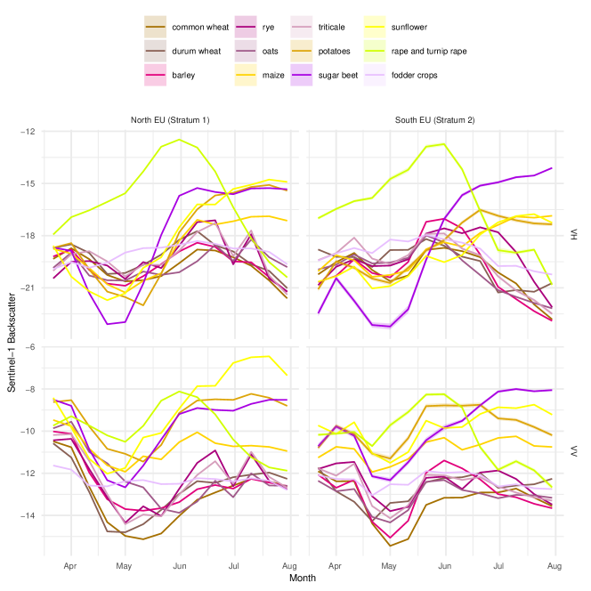
Fig. 3: Evolution of VV and VH backscatter for the growing season for the 12 main crops. The value are averaged per stratum. The ribbon around the line corresponds to one standard deviation.

Fig. 4 summarizes the overall accuracy through time. An initial steep increase in accuracy is observed from February to June when only very small increases are achieved by adding more data. By the end of July the accuracy reaches a value of 78.8% (Fig. 4).

The dynamic of the Fscore through time for each crop separately (Fig. 5) shows expected patterns. The rape and turnip rape Fscore is booming when the crop is flowering in May (Fscore 0.86) indicating that the model could identify them quite early in the growing season (March). The figure also shows that common wheat has a steep increase in Fscore in April which coincides with the reproductive growth period. Grain maize, a summer crop which is harvested later in the season than winter wheat and rape and turnip rape, is reaching the plateau in Fscore at the beginning of July. Interestingly, the Fscore for sugar beet continuous to increase until October which is logical as sugar beet is harvested in late autumn in Europe. Finally, as expected, we observe a very low Fscore value for mixed classes (such as other fodder crops).

As detailed earlier, and considering also any future operational application, we opted for using time-series from January until the end of July for further processing (evaluation of indices and final training of the RF algorithms).

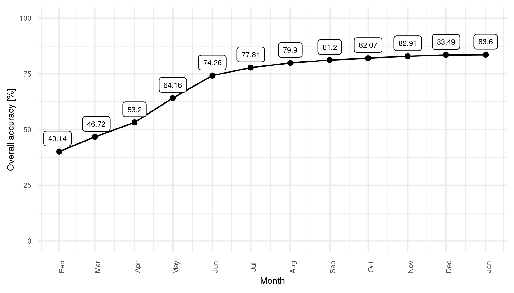
Fig. 4: Overall accuracy at a monthly time step for the crop type level and the two strata combined

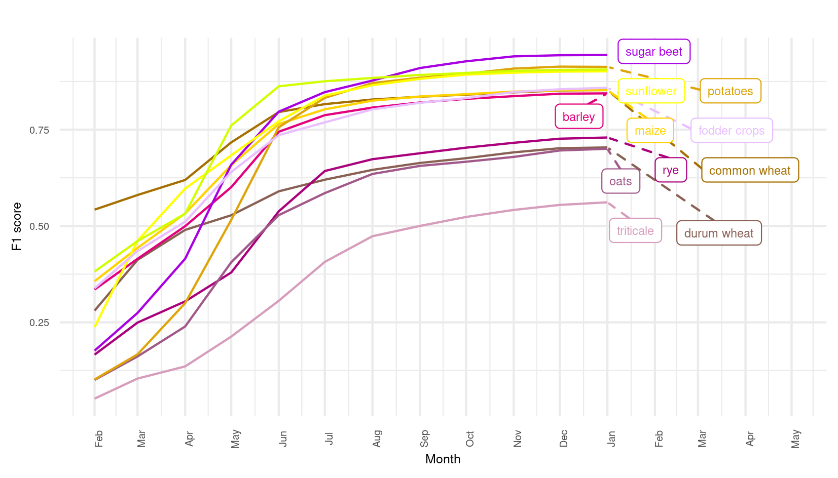
Fig. 5: Evolution of The F-score through time for the 12 mains crops over the EU-28.

From the comparison (Table 3) of the overall accuracy for the polarization backscattering coefficients (VV and VH), the cross-ratio index (VH/VV) along with their combinations, we observe that the combination of VV and VH gives the highest accuracy (79.89 %) and is selected for the EU crop map. The training data for the EU crop map therefore consists of 10-day time series of VV and VH backscatter coefficients from 1st of January to 31st of July (22 dekads).

Table 3: Overall accuracy for S1 indices (dates are fixed from Jan to end of July).

Indice	Overal Accuracy
VV	71.96
VH	72.70
VH/VV	50.90
VV and VH	79.89
VV and VH and VH/VV	77.91

3.2 Crop type over EU

3.2.1 Visual assessment

The EU crop map presented in Fig. 6 is representative of a number of crop types and main vegetation classes and covers 91 Mha of cropland (9,174 M 10 m pixels). The map is available for download and visualization (see section Data dissemination).

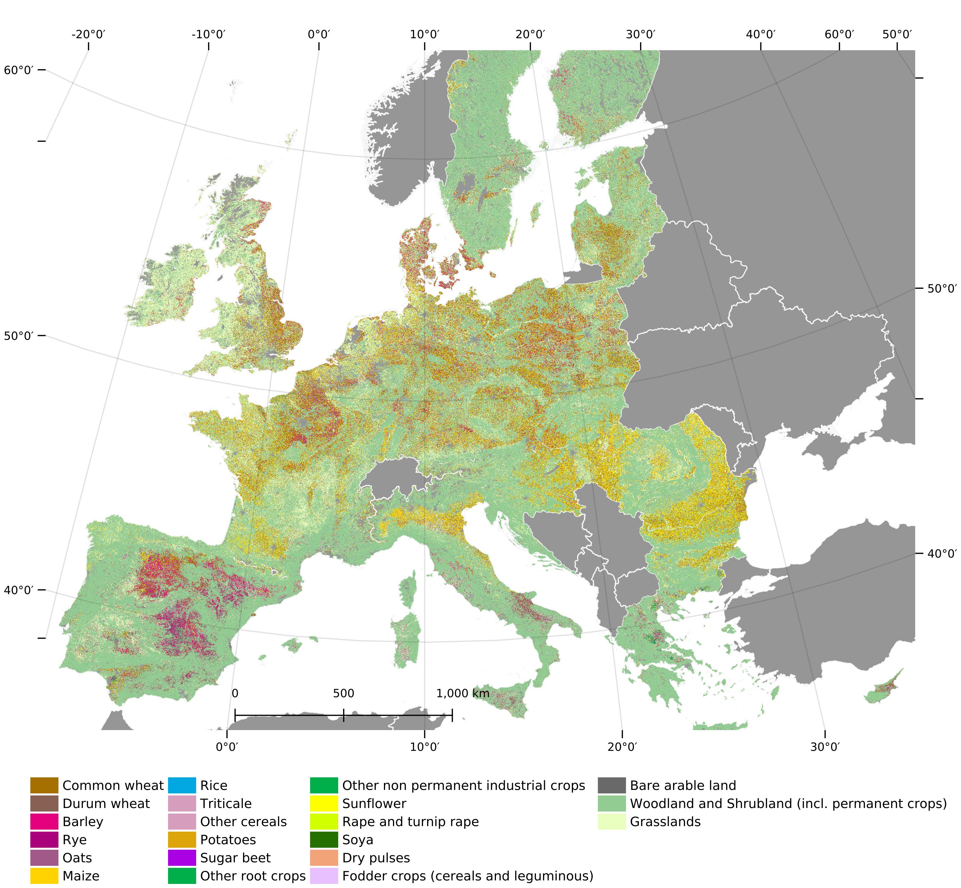
Fig. 6: EU crop type map for 2018.

The resulting map is consistent over different landscapes at the level of the main land cover classes. A naive area estimation by pixel counting for each class is provided in Supplementary Table S5. Woodlands and shrublands are regrouped in a single class covering more than 2 M km²; i.e. more than half of the area mapped because it is a very broad class covering broadleaved and needleleaved natural and managed forests as well as permanent crops. The arable land class has an extend of about 0.9 million km². The grassland class, grouping the permanent and temporary grasslands covers 0.7 million km². The woodland and shrubland class covers forests patches but also tree lines and hedges in agricultural landscapes.

Over the EU-28, the three most detected crop types in term of area are common wheat, maize and barley. Despite using a pixel based classification approach, separated parcels can clearly be recognized. The difference in the size of parcels is well captured, as illustrated in Fig. 7, by comparing Fig. 7 (b) Austria and the Czech Republic Fig. 7 (c). The crop types are identified over the EU without a priori knowledge of country practices. The ability of the map to represent different agricultural landscapes is well illustrated in the examples of Fig. 7 for North of Orleans, France (a) where the diversity of crop types cultivated in the area are distinctly classified (wheat, barley, sugar beet, maize, potatoes, rape and turnip rape, dry pulses). North West of Valladolid, Spain Fig. 7(c) the major crops cultivated in Castilla y Leon: barley and sunflower are clearly detected together with some parcels of wheat, dry pulses and bare arable land. In Romania, North East of Bucharest Fig. 7 (d), the diversity of small and large parcels of wheat, maize, rape and turnip rape, sunflower and barley are well captured.

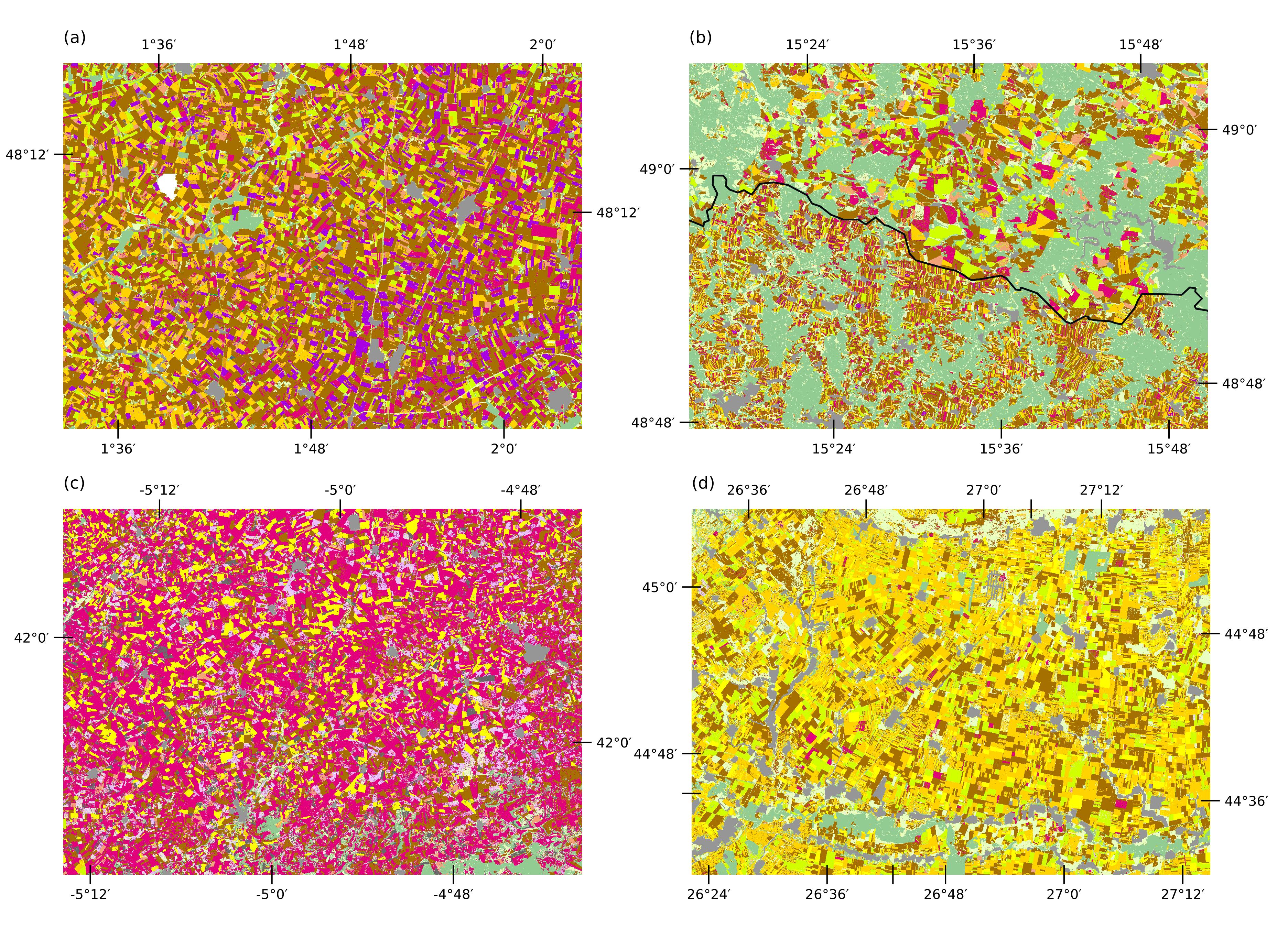
Fig. 7: EU crop map for (a) Orleans (France), (b) border between Austria and Czech Republic, (c) Castilla and Leon (Spain), (d) (Romania).

3.2.2 F-score per crop type and administrative unit

As agricultural practices vary across Europe, in terms of crop type cultivated and crop calendar, we expect our mapping approach using a minimal stratification to represent the field reality with different fidelity in different areas. To investigate this aspect, a first assessment of spatial discrepancy for arable land class accuracy is done by calculating the F-score at country level, when enough LUCAS points were available, for the six main crops over EU, i.e. common wheat, barley, maize, sugar beet, sunflower, rape and turnip rape. This allows to quickly grasp how well the classification is performing spatially as highlighted in Fig. 8 (see Supplementary Table S9 for number details). The F-score for most crops is higher in the northern part of the study area than in the southern part. The F-score for common wheat is about 0.7 for Belgium, Bulgaria, Czech republic, Denmark, France, Luxembourg and Slovakia. Maize reaches high scores in the North (above 0.8 for Germany, Czech Republic, Hungary and Slovenia) and rape and turnip rape have an F-score higher than 0.9 in Austria, Czech Republic, Germany, Lithuania, Luxembourg, Latvia, Poland and Slovakia.

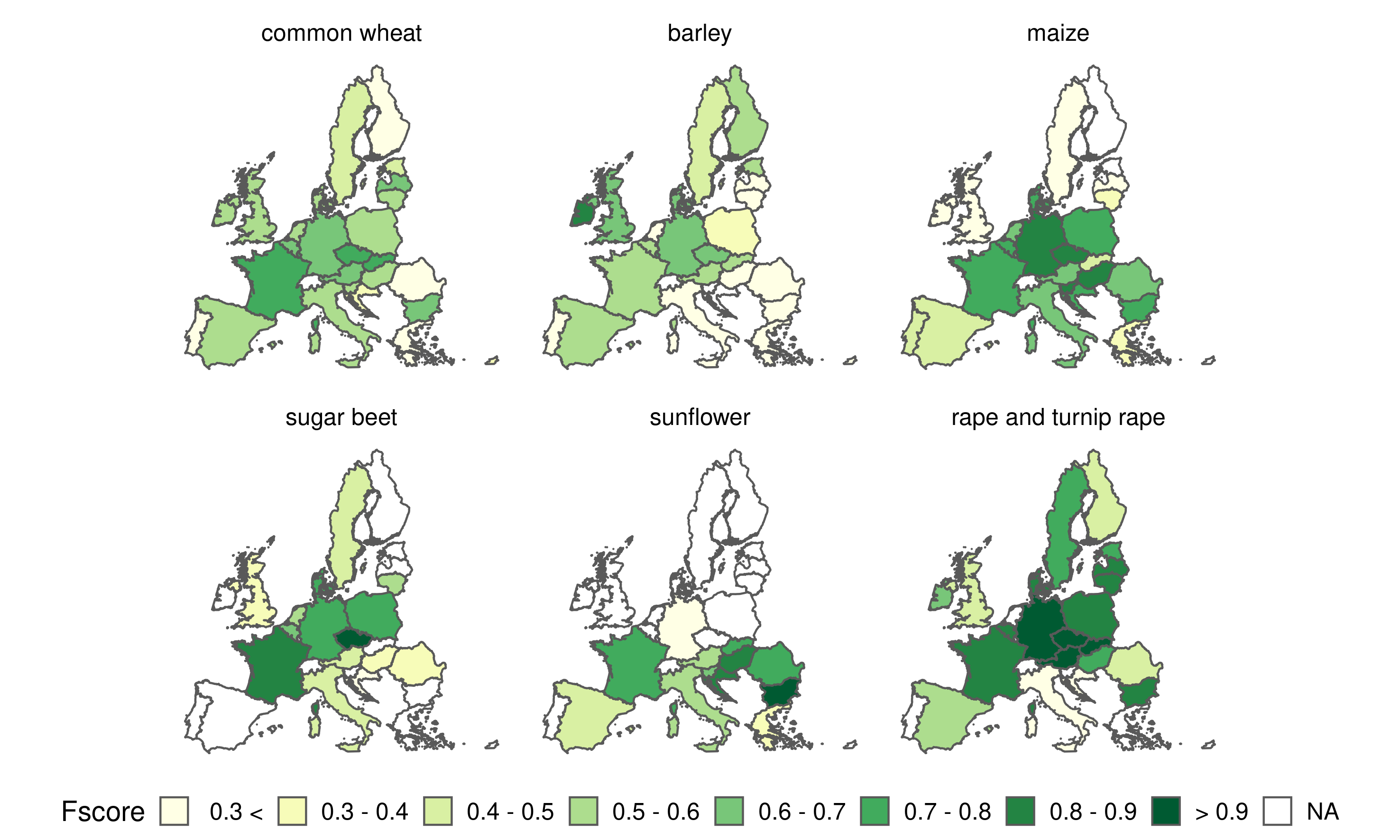
Fig. 8: The F-score per country for the 6 main crops in Europe.

3.3 Accuracy Assessment

3.3.1 LUCAS core points

The accuracy of the EU crop map is evaluated using $87.853$ points selected from the LUCAS 2018 survey. An overall accuracy of 76.1% (Supplementary Table S2) is achieved over the EU when considering the 19 crop type classes with the woodland and shrubland and grassland classes. An accuracy of 80.3% (Table 4) is achieved when grouping the crops by the main crop type classes (groups defined in the Table 1). The woodland and shrubland class is well discriminated from the rest (PA of 97% and UA of 83%). A confusion is observed between the grasslands class and the woodland and shrubland class, as highlighted by a PA of 58% for grasslands indicating an omission error. The UA of grassland is 82% indicating a commission error for grassland and again a confusion between the grassland and woodland and shrubland class. The pixels mapped as woodland and shrubland instead of grassland and vice versa could be linked with the class definition of woodland and shrubland including open tree/shrub cover canopy (10%). In terms of land cover some classes of grasslands are very similar to open canopy class of woodland and shrubland. The point information provided by the LUCAS core dataset is also not the most suitable to assess more complex land cover classes characterised by discontinuous canopies.

Regarding arable land, cereals are well discriminated, reaching a producer accuracy (PA) of 84% and user accuracy (UA) of 72%. Omission errors for the cereals class are mainly occurring with the woodland and grassland classes while commission errors are happening mainly with grasslands. Root crops have a lower PA of 59%, with many points labelled as root crops being mapped as cereals instead. However the root crops present a high UA of 90% showing little commission errors with the other classes. The non permanent industrial crops have high PA (89%) and UA (79%) with good discrimination of sunflower and rape and turnip rape. The fodder crops class including cereals and leguminous cultivated for fodder is not well discriminated and is confused with the cereals and grassland class (PA of 7% and UA of 29%).

Regarding specific crop type (Table 5), the LUCAS accuracy assessment highlights a difference between the northern and the southern stratum with an OA of respectively 78% and 70.8%. The overall best-performing crop classes are rape and turnip rape, sunflower and maize. In the northern stratum, common wheat, maize, sunflower and rape and turnip rape have PA above 80% but the value of their UA is lower, indicating commission errors. The commission error is specifically high for the common wheat.

Table 4: Confusion matrix for crop type group class for the EU-28. The values represent weighted area UA Users accuracy PA Producer Accuracy.

		Reference class (LUCAS point)
	Map Class	210	220	230	240	250	290	300	500	UA (%)	SE (%)	OA(%)
210	Cereals	0.13	0.003	0.002	0.002	0.005	0.009	0.002	0.026	72.3	0.6	80.3
220	Root Crops	0	0.006	0	0	0	0	0	0	90.1	2
230	Non permanent industrial crops	0.001	0	0.024	0.002	0	0.001	0	0.001	79.5	6.2
240	Dry pulses, Vegetables and Flowers	0	0	0	0.002	0	0	0	0.001	43.6	4.4
250	Fodder Crops	0.001	0	0	0	0.001	0	0	0.002	28.8	3.3
290	Bare Arable Land	0.001	0	0	0	0	0.006	0.001	0.003	50.3	2.7
300	Tree and Shrub Cover	0.01	0	0	0.001	0.004	0.004	0.483	0.077	83.4	0.4
500	Grassland	0.01	0	0	0	0.009	0.001	0.013	0.151	82.1	0.5
	Producer accuracy (%)	84.4	58.6	89.3	23.6	6.9	25.7	96.9	58.1
	Standard Error (%)	0.8	3	1.3	3.9	0.8	1.7	0.1	0.6

Table 5: Weighted area accuracy metrics, overall accuracy for the crop types classification (level-2) and producer and user accuracies for the main crop type classes (for the whole study area and for the two strata)

	All		stratum 1		stratum 2
class	P.A.	U.A	P.A.	U.A	P.A.	U.A
common wheat	78.2	49.6	82.5	49.9	44.5	46.0
durum wheat	25.9	49.7	1.8	92.3	45.2	49.0
barley	53.8	51.6	50.0	57.8	67.2	44.2
maize	84.0	58.5	87.6	58.3	22.7	66.7
potatoes	37.3	73.5	39.8	74.1	\	\
sugar beet	57.1	75.0	57.9	75.0	\	\
sunflower	86.7	62.2	90.7	72.0	64.3	32.4
rape and turnip rape	82.7	80.2	83.5	80.2	17.9	78.9
Overall accuracy	76.1		78.0		70.8

3.3.2 GSAA

The LUCAS core points are giving a first evaluation of the accuracy of the crop type at the continental level. A more detail assessment is done with the GSAA data for specific countries or regions. For each region, the classified crop of each parcel from a crop representing an area greater than 1% of the region is compared to the one from the GSAA. After removing the grassland and woodland classes the confusion matrices are computed. The confusion matrices along with the PA and UA for each region are presented in Supplementary Material see (Supplementary Table S11 for bevl2018, Supplementary Table S12 for dk2018, Supplementary Table S15 for nld2018, Supplementary Table S16 and Supplementary Table S13 for si2018). The PA and UA for the main crops are summarized in 9(a) and 9(b) respectively.

The analysis shows very promising results for the detection of common wheat, barley, maize, sunflower and rape and turnip rape in all the regions analysed. Rape and turnip rape are detected without almost any confusion in the three regions where it is present (dk2018, frcv2018 and nrw2018), reaching PA above 98% and UA above 97%. It is worth noting that common wheat and barley have much better accuracies for both PA and UA compared to the LUCAS points based assessment, with the exception of si2018. Except for nrw2018 and si2018, common wheat has a PA above 80%, while the UAs are above 92% in all regions except si2018. In nrw2018, the most common confusion for common wheat are omission error towards barley and triticale classes. On the other hand any parcels of triticale in GSAA are correctly mapped as triticale. The confusion of common wheat with triticale is due to the similarity of the two crops, both in general crop structure and seasonality. In si2018, omission errors are observed towards barley and the other cereals class. Barley is present in the six regions with a PA above 92% except for dk2018 (88%) and nld2018 (82%). In Denmark, this is explained by a confusion between common wheat and barley while in nld2018 the confusion is mainly with maize. The UA for barley are a bit lower than the PA value but still above 80% for bevl2018, dk2018 and frcv2018. Both in nrw2018 (UA 76%) and nld2018 (UA 64%), the main commission error is due to a confusion with common wheat. Sugar beet presents very promising results in bevl2018 (PA 97% and UA 93%) and nrw2018 (PA 84% and UA 85%). In bevl2018, dk2018 and nld2018 where UA are lower, the confusion is mainly with maize and to a lesser extent with potatoes. The class potatoes, presents in four regions, shows high PA (91% in bevl2018, 96% in dk2018, 95% in nld2018 and 94% in nrw2018) and relatively low UA. In nrw2018, dk2018 and bevl2018, the UA (respectively 47%, 54% and 50%) of potatoes is explained by commission errors with maize. However, the UA of maize is showing little commission errors (99%). In nld2018, confusion is happening with maize and sugar beet and probably linked to the time period made available to the classifier. Maize and sugar beet maturity phases are reached in autumn, between September and November. A better discrimination would thus be expected later in the season.

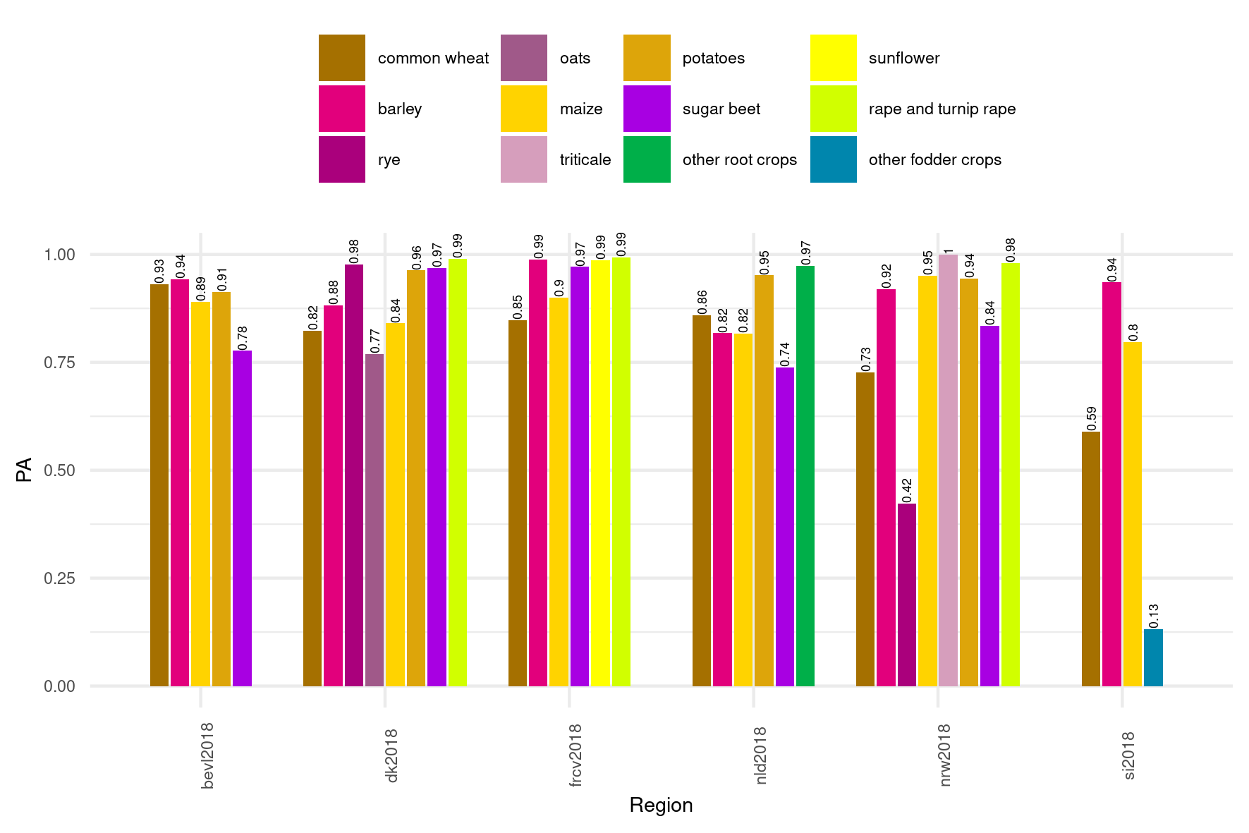
(a) PA

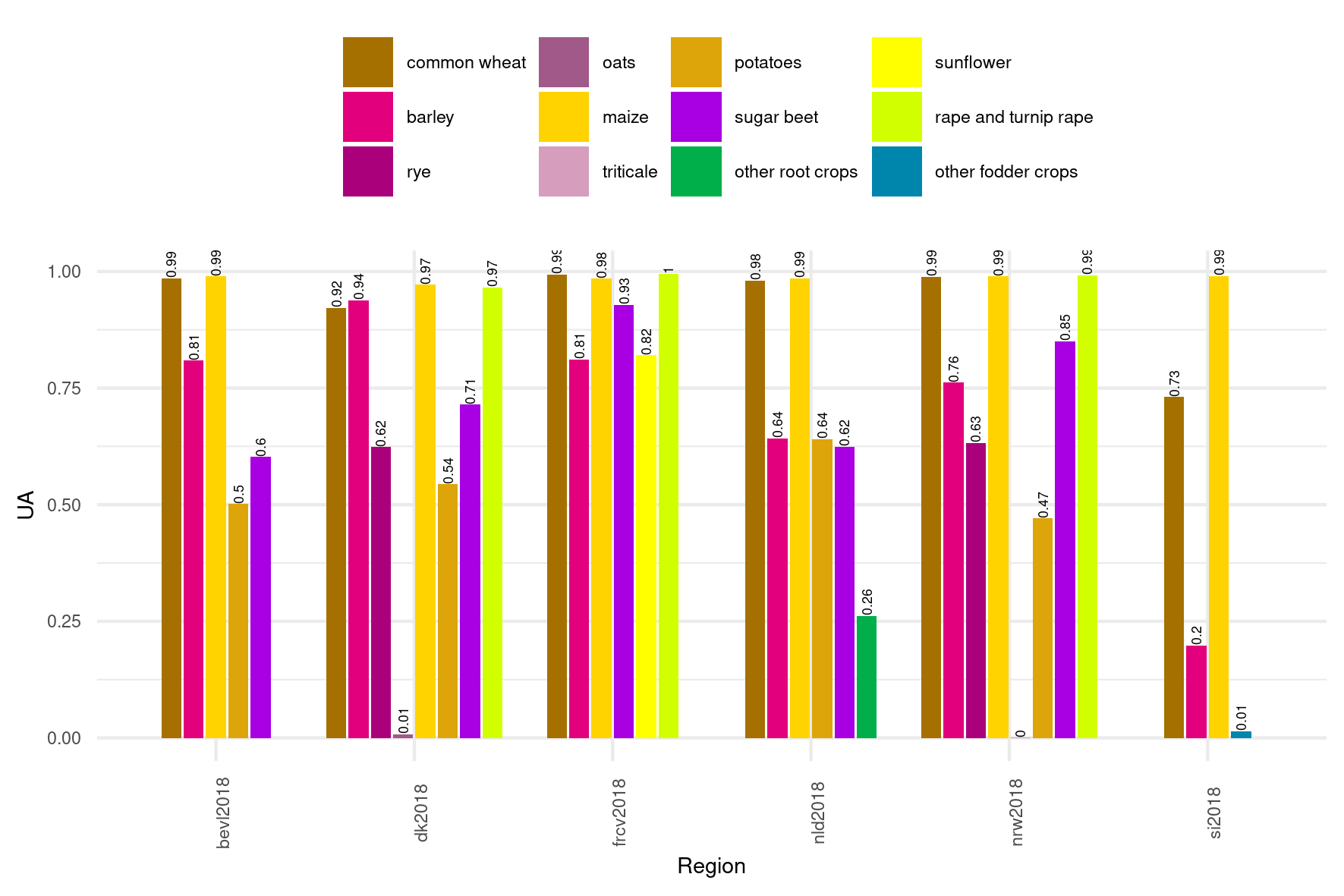
(b) UA

Fig. 9: User and Producer accuracy obtained from the comparison of the EU crop map and the parcel data from the GSAA. The detailed confusion matrices are in Supplementary Material.

3.3.3 Subnational statistics

The crop area data is extracted and compared for 220 administrative regions covering most of the EU-28. The matching with the reported statistics was done at the NUTS2 level(Supplementary Table S17). For DE and UK no data is available at NUTS2 level, the comparison was thus done at NUTS1 level for which statistics are available. Fig. 10 shows how the area estimated by the EU crop map compared with the area reported by Eurostat. The calculated Pearson’s correlations (r) range from 0.93 for potatoes and rye to 0.99 for rape and turnip rape. Additionally, the relative difference in area (%) is computed for each region and presented in Supplementary Fig. S5 (Supplementary Fig. S6 provides the histogram of the differences for each crop). The maps show that while for common wheat and maize the EU crop map estimations are generally higher compared to Eurostat without a distinct spatial pattern in observed differences, this is not the case for other crops, whose overestimation and underestimation are more localised. Barley for example is underestimated in the center of Europe but overestimated in both the north and the south of Europe. The distribution of the difference shows that common wheat and maize are underestimated in our EU crop map compared to Eurostat. Barley is under-estimated in the northern part and over-estimated in the southern part. The other main crop area estimations are close to the official Eurostat statistics.

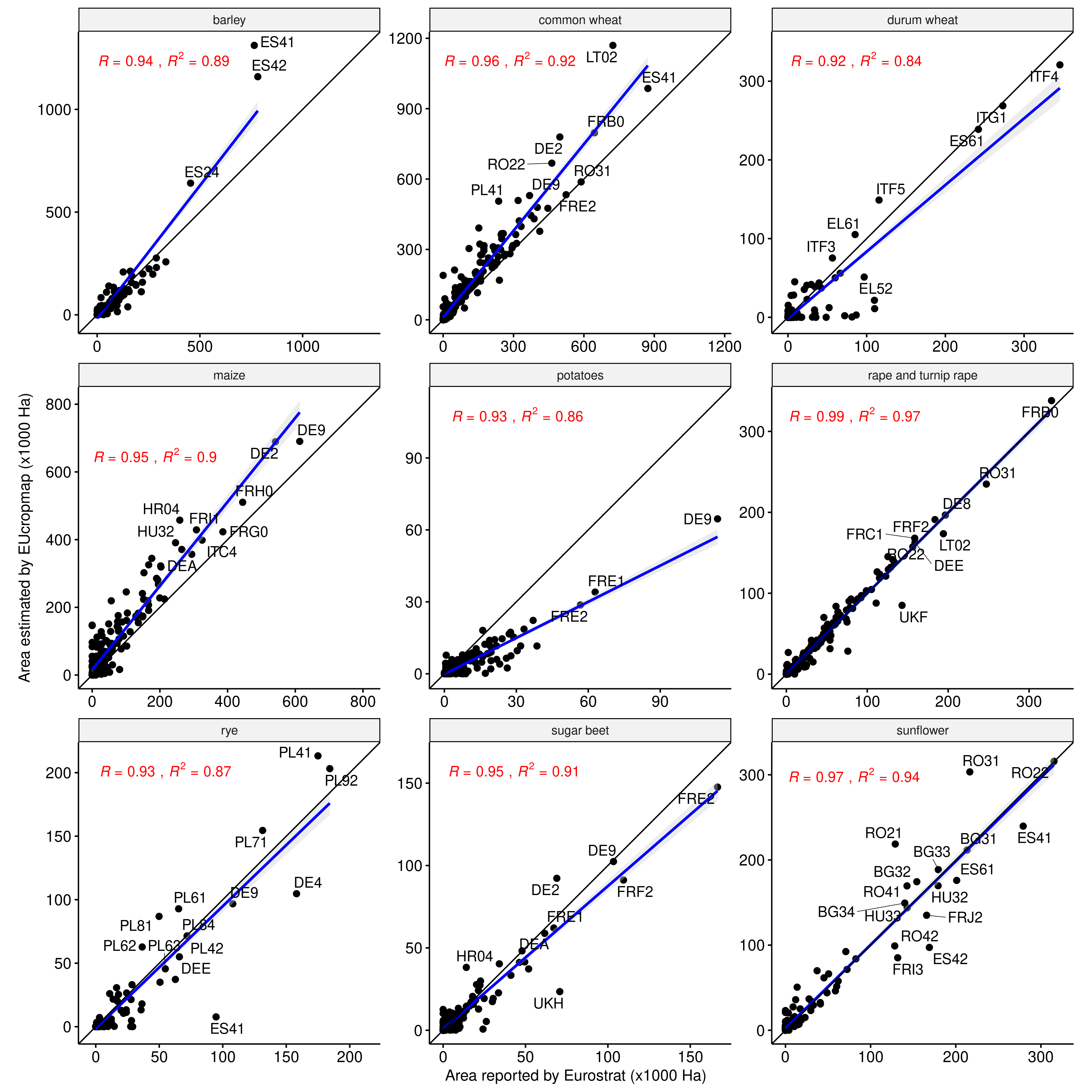
Fig. 10: The areas reported by Eurostat at NUTS2 level (except for UK and DE at NUTS1) are compared with the area retrieved from the EU crop map. $R$ is the Pearson correlation coefficient, $R^{2}$ is the the coefficient of determination.

4 Discussion

4.1 Timeliness and accuracy of the crop type classification

The final map presented in this study is built with S1 observations from January to end of July. The overall accuracy at the end of July across all crops is relatively high at 76%. As the season progresses, discrimination of crop types and parcels keeps improving as shown in Fig. 11. However, for an operational application specific crops can be mapped earlier during the season depending on the specificity of the region and requirements regarding accuracy for specific crop types. The timing when the F-score is highest for each specific crop is linked to canopy structure and phenological stage as these affect the backscattering signal. For in-season applications, a trade-off can be found between the required level of accuracy and timely map production.

While covering only 2018, the current study shows potential for developing in season prediction of crop type and confirms the observations of [Veloso et al., 2017, You & Dong, 2020] at the EU scale. A key element is that the S1 SAR signal is not affected by atmospheric perturbation. Any acquisitions can thus be used for crop type mapping. Although dependent on year to year phenological development, findings regarding the best timing for specific crop types are likely to be valid for future studies.

Supplementary Fig. S7 shows that the time series of VV and VH backscatter for specific crop types have a similar shape in the northern and the southern stratum but often appear shifted in time. This relates to phenological development that occurs later when going northward. As a consequence, the F-score for the same class may peak at different times as revealed by the analysis of the temporal evolution of the F-score in the two strata.

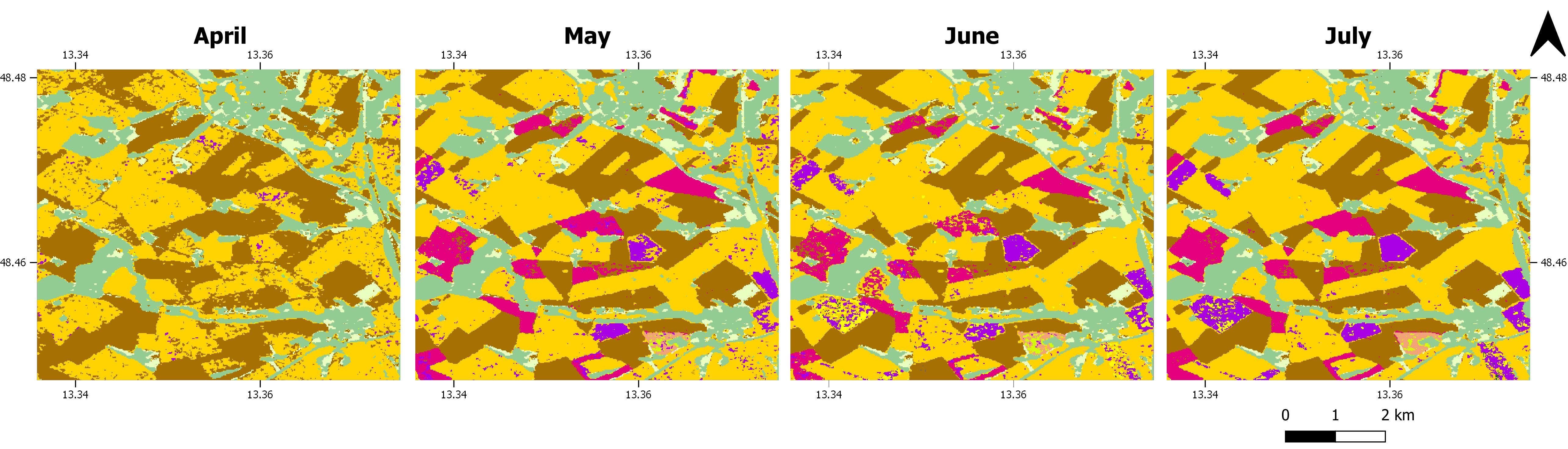
Fig. 11: Crop type mapping results for different time periods, considering the data from January to respectively April, May, June, and July (the EU crop map presented in this study) in South East Germany.

In the northern stratum (Supplementary Fig. S1), the F-score reaches a plateau at the end of June for common wheat, rape and turnip rape. Other cereals (rye, barley and maize) can be predicted with a high F-score at the end of July, even if the F-score keeps increasing slightly until the end of the summer. The F-score for sunflower, potatoes and other fodder crops reaches a plateau one month later, at the end of August, while sugar beet reaches the plateau in September, in agreement with its longer growth cycle that extends into autumn. Winter wheat and rape and turnip rape that are already established in the field at the beginning of the year, present a structure, reflected by the VV and VH backscatter, that is already different for the other classes earlier in the year.

Similar results were found in other studies exploring the potential of S1 for crop type monitoring in northern European countries. For Belgium, Van Tricht et al. [2018] illustrates that while winter cereals were already well discriminated at the end of June, end of August was more appropriate for potatoes, maize or sugar beets. For France, Veloso et al. [2017] showed that S1 backscatter clearly separates winter wheat and rapeseed between March and July during the tillering and senescence stages and distinguishes maize, soybean and sunflower during the heading/flowering phase between June and the end of August.

In contrast, the highest accuracies are achieved earlier in the Mediterranean stratum. Already at the end of June, plateaus in F-score are reached for the accuracies of wheat (common and durum wheat), rape and turnip rape, other fodder crops, and the mixed class ”other non permanent industrial crops” (including e.g. cotton, fibre and oleaginous crops). At the end of July, the plateau is reached for barley, sunflower and root crops while it is reached end of August for maize. The earlier time at which the highest accuracies are achieved in the southern stratum can be explained by typical timings of the growing season in the two strata. As shown in (Figure S4) Meroni et al. [2021] there is latitudinal gradient in the timing of the growing season with earlier growing seasons in the south of Europe. This gradient justifies the observed lag in achieving the best performances in the two strata

To assess the accuracy of the EU crop type map produced at the end of July, three different and complementary approaches were presented in the Section 3.3. We discuss here the pros and cons of each.

The first one using high-quality LUCAS points (Section 3.3.1) enables an accuracy assessment for the whole continental area but on the other hand the protocol to collect the in-situ information is not designed for EO applications and we filtered out ”low-accuracy” points, working only with a subset of the 2018 survey. In addition, the point information is difficult to reconcile with the assessment of crop type classes that present spatial heterogeneity in a small area and especially where only few acquisitions contribute to the 10-day average (e.g. in the South). Speckle filtering, not used in the present study, may attenuate such undesired heterogeneity.

The information about the crop type is then assessed more precisely with the GSAA (Section 3.3.2). The main differences between the LUCAS point based and GSAA parcel based accuracies are due to the parcel aggregation of the pixel classification within the GSAA parcel, which uses a majority filter. In this way, the analysis is not deteriorated by possible geometric inaccuracies that can affect the LUCAS points. In addition, speckle-induced variation affecting the pixel classification result within the parcel is removed. However, the GSAA assessment is limited to specific areas in the northern part of the study, due to a lack of openly accessible GSAA sets for 2018.

Finally, the comparison with the official statistics (Section 3.3.3 ) has the obvious advantage of covering the whole area of interest but the drawback of being a rather coarse evaluation of the classification as the comparison with official statistics can only be performed at some aggregate administrative spatial level.

Useful observations can be derived from the comparative analysis of of the three complementary level of accuracy assessment. For instance, some specific errors are detected with all approaches.

From the comparison with official statistics (Fig. Supplementary Fig. S5 and Supplementary Fig. S6) we observe an overestimation of common wheat in the northern part of our study. Similarly, for common wheat, an important commission error with other cereals classes is depicted by the LUCAS points assessments. The same confusion (common wheat versus barley and triticale) is reported by the GSAA assessment even with a smaller severity.

An over-estimation in the northern stratum is also observed for maize. This is consistent with what is observed in the accuracy assessment based on the LUCAS point(a low UA associated with an important commission error). In contrast, this is not reported in the GSAA assessment where the high UA of maize illustrates a low commission error for that class. Contrastingly, an under-estimation of maize is observed in the southern part of our study area. This is in agreement with the omission errors reported in the LUCAS assessment. We however lack of the GSAA comparison in the South to confirm this observation.

While barley is over-estimated in the southern part of the study, it is under-estimated in the northern part according to the official statistic assessment. The underestimation of barley in the North is in agreement with the LUCAS point assessment reporting low PA and UA. In contrast, the GSAA assessement reports PA are above 80% in all GSAA analyzed, not confirming an omission error. An hypothesis is that the GSAA assessment filters the pixels that are not yet detected as barley at the parcel level. The overestimation of barley in the South is confirmed by the LUCAS point assessment.

The confusion observed at the level of the study area with the LUCAS points assessment (Table 4) between the cereals and the root crops and for the GSAA between sugar beet and maize and potatoes is directly related to the time period (January to end of July) selected for EU crop map. The evolution of the VH backscatter coefficient in time Supplementary Fig. S7 illustrates what is also visible from the F-score Supplementary Fig. S1, that the discrimination between broad leaf crops, cereals and maize increases from June onwards in the Northern stratum. Extending the period of a few month would alleviate these problems.

4.2 Recommendation for an operational service

More than 6 years after the successful launch of the first Copernicus satellite, S1 A, Europe still lacks access to a full, free and open archive of Level-2 Copernicus Application Ready Data for the S1 (A and B) sensors (S1-CARD). Whereas Sentinel-2 Level-2 data is produced as a routine ESA output, this is not the case for S1. Level 2 S1-CARD generation is a required expensive processing task that should be done once with the results made available to the community.

The scale of this study requires the use of advanced cloud computing solutions closely coupled to the massive on-line data archives of Sentinel data. The requirements for such cloud solutions are that they provide access to application ready data (ARD) and a programming interface that allows the application of advanced machine learning algorithms, for instance, in support of supervised classification, as was applied in this study. GEE is currently the only platform that provides access to consistently processed S1 ARD (backscattering coefficients only, for now), which is processed with a standard recipes using the open source SNAP s1tbx software. Nevertheless, although GEE offers a number of routines for supervised classification (including RF used in this study), it has some limitations in the hyperparameter tuning along with some processing issues when the model is applied to very large areas. This is why the pre-processing of the S1 data into 10-day temporal synthesized mosaics was done in GEE while the results were downloaded on a local facility to perform the classification. For this study, this represented about 10 TB of data. This data transfer is clearly sub-optimal and, in addition, while GEE is free to use for non commercial application, the download of large amount of data has to be done via a paid Google Cloud account. In our study, we have processed the annual volume of data for 2018 in a post-hoc fashion (i.e. the classification was done off-line after the growing season). However, with the effective use of cloud based solutions, our method can be run in quasi-real time, for instance as a combination of transfer learning with early season in situ collection and GSAA for training and testing. Cloud based capacities allow integration of daily acquisitions in 10-day compositing with automatic re-run of the ML classifiers. Deep learning approaches that learn to extract discriminative temporal information from the data, such as convolutional Neural Networks and Recurrent Neural Networks could provide a more robust alternative to RF and should be considered for further studies.

Finally, it is interesting to reflect on the actual utility of a EU crop map against other potential sources. We in fact acknowledge that there would be no need for a post-harvest crop map with 70-85% accuracy for only a limited set of major crops if the annual GSAA declaration set is available in July, with a typical accuracy of 90-95% (for a far more significant set of crops). However, so far, most of the EU Member States’ GSAA are not openly accessible and, when this is the case, they are usually available after the growing season (the Netherlands being an exception, with a preliminary version published in July of the current year). Recently, the Integrated Administration and Control System (IACS) spatial data sharing initiatives is promoting EU member states to share their IACS data within the infrastructure for spatial information in Europe (INSPIRE) portal. The expected outcome of this new regulation is the expanded public availability of GSAA.

While LUCAS is performed every three years, the GSAA data are collected every year in Europe, making them and ideal source of ground data for crop classification training and validation. Beside the legal and technical challenge to make the data open access already discussed, the legend semantic harmonization is key to use in classification approaches across different regions. While the semantic matching was done for this specific study, a common semantic model would be very useful to integrate GSAA in a more detailed EU-wide classification context.

Besides LUCAS and GSAA, other information source could be considered. The use of crowd sourcing to collect in-situ data and generate LUCAS-like information could enrich data availability [Laso Bayas et al., 2020]. The use of geo-tagged street-view pictures has been already investigated for agriculture monitoring [d’Andrimont et al., 2018b] and could represent an alternative in-situ dataset. Application like Pl@ntnet [Joly et al., 2016] or i-naturalist [Van Horn et al., 2018] collect massive plant and species occurrence information via their portal. Finally, leveraging mobile gaming solutions such as the impact games (https://world.game/) could represent an additional alternative to collect massive in-situ data.

4.3 The EU crop map 2018: perspectives for improvement

There are a number of limitations in the proposed mapping approach. Some are coming from the lack of information in the LUCAS survey and other from methodological choices.

From the LUCAS data, the limitation comes mainly form the crop type surveyed, the number of samples per classes and details about the agriculture practices such as irrigation. We did not distinguish between rain-fed and irrigated parcels due to a lack of samples in each category. This particularly affects the maize detection in the South of Europe where most of the maize is irrigated. The Supplementary Fig. S5 shows that the maize is indeed underestimated in Spain, southern Italy and Greece. Another limitation is that the approach proposed doesn’t capture rice. While that class is usually easy to discriminate from other crops, it is here missed due to the lacking of training data (i.e. 14 polygons). The west area of northern Italy is particularly affected, with a confusion between rice and maize. Future studies could consider using information about the water management available in the LUCAS survey. Better understanding and taking into account on the backscatter signal of irrigated surfaces would also certainly improve the discrimination of irrigated crops.

In term of methodological choices, improvements are possible taking into consideration crop classes not considered in this study. Specifically, permanent crops are covering a considerable extent of agricultural land and are currently classified in the broad class Woodland and shrubland. The Copernicus information for the two classes of permanent crops (fruit trees and the other permanent crops such as olive and vineyard) can be used to explore classification workflows identifying them. Distinction between temporary, permanent and natural grasslands would also be worth considering in future developments which would include multi-season temporal profiles.

Although we have not considered using S1 coherence in this study we are well aware of the potential use of this alternative Level 2 product in agricultural use contexts (e.g. Tamm et al. [2016], De Vroey et al. [2021]) . We realize that a future extension of S1 use in national or continental crop mapping requires the introduction of terrain flattening to better compensate for incidence angle and look direction differences in the multi-orbit compositions for 10-day periods. Although we have masked terrain with steep slopes ($>$ 10^∘) above 1000 m limiting these effects somewhat, we expect improvements especially for crops with an extended bare soil phase (e.g. summer crops) for which angular variability in backscattering can be significant. We have not applied speckle filtering, because speckle variance is already reduced in the averaging step we apply to create the 10-day composites and using polygon averaged values for the RF training. However, the sparser revisit frequency in the Southern areas makes speckle filtering potentially useful. Furthermore, we could consider speckle filtering with a shorter averaging period (e.g. 5 days) in the North, to better capture abrupt temporal changes in the $\sigma^{0}$ signatures (e.g. at harvest).

This study demonstrates the potential of S1 as a baseline for continental mapping. However Sentinel-2 (S2) would certainly improve the results as already demonstrated by Van Tricht et al. [2018], Gao et al. [2018], Kussul et al. [2018], Orynbaikyzy et al. [2020], Chakhar et al. [2021]. In particular, we expect that the inclusion of S2 data would improve the discrimination of main cropping practices. For example helping to separate winter crops from permanent grassland, for the detection of bare soil conditions in spring to delineate summer crops, and to highlight crop specific phenology events (e.g. d’Andrimont et al. [2020a]). Additionally, S2 would be particularly useful in the South where there is less cloud coverage and also less S1 acquisitions [Lemoine, 2017]. More generally, to facilitate S2 ingestion in the machine learning processing, smoothed time series of cloud free biophysical variables would be useful (e.g. the Copernicus pan-European High-Resolution Vegetation Phenology and Productivity products (HR-VPP) [Tian et al., 2021]).

The EU crop map provides a coherent and unique continental view with a spatial detail that is relevant for crop management interventions at the parcel level. As such, the information can be relevant for EU wide policy monitoring, e.g. by deriving indicators such as crop diversity [Merlos & Hijmans, 2020], and be a source of input data for EU wide models and assessments requiring detailed information on crop location.

Another perspective is to derive national or sub-national area statistics from the EU crop map. This was not considered in this study. Area estimation can be done directly from the crop map (pixel counting) but this is not taking into account the bias inherent of remote sensing: the presence of mixed (border) pixels and the misclassification of pure pixels Gallego [2004]. Estimating area from a satellite-based map typically requires the use of an un-biased estimators [Olofsson et al., 2014, Stehman, 2014, Gallego & Delincé, 2010] by combining data from a ground survey or from another source of higher quality data in combination with the map. LUCAS 2018 survey is a source of reference data, providing information until the NUTS2 level. However, further exploration is needed in order to use it for area estimation at a finer scale. While the approach of Gallego & Bamps [2008] for area estimation with CLC as post-stratification could be a first naive approach, a more precise approach would be the one of Stehman [2014] to take into account the fact that the strata from our map and the strata from the LUCAS survey are not similar. However, for this purpose, the sampling weight of each LUCAS point should be made available by Eurostat. In addition, further care should used to account for the fact that a subset of the 2018 survey was used in the training.

This study sets up a framework that could apply for other years. While the approach demonstrated is robust, using model trained for 2018 on other years could result in not satisfying result. Indeed, it is noted that 2018 was a peculiar year, with droughts and severe heatwaves affecting Europe. Drought conditions in central and northern Europe caused yield reductions up to 50% for the main crops, yet wet conditions in southern Europe saw yield gains up to 34%, both with respect to the previous 5-year mean [Buras et al., 2019, Toreti et al., 2019]. To tackle year to year seasonality and the limited availability of in-situ data, classification methodological developments are still needed to apply the proposed approach to other years.

5 Conclusions

Arable land represents almost half of total EU area and its monitoring is crucial for efficient environmental, agriculture and climate policies’ implementation. In this study, a framework to derive a 10-m crop type from S1 at continental level has been designed, implemented and assessed rigorously. The proposed framework opens avenues to develop a synergistic robust information system to monitor agriculture consistently both at fine spatial-and-temporal scale over large areas. This demonstrates the current momentum combining the unique Copernicus Sentinel fleet, high quality massive in-situ data along with cloud computing. The method and data developed will serve communities ranging from scientific modellers to policy makers.

6 Author contributions

R.D and A.V conceptualized the study and designed the methodology, R.D., A.V., G.L., P.K. processed the data. R.D., A.V., G.L., P.K., M. M. , M. V. analyzed the data and wrote the paper.

7 Acknowledgements

The authors would like to thank Kostas Anastasakis as jrc-cbm developer, Javier Sanchez Lopez for his agronomicic advices, the JRC JEODPP colleagues for their continuous support and the Google Earth Engine team for their technical help.

Data dissemination

The EU crop map masked with the non-vegetation classes and steep slopes is available for download and visualization.

Contents

1. 1 Introduction
   1. 1.1 Crop mapping with Sentinel-1
   2. 1.2 In-situ data in the European Union
   3. 1.3 Objectives
2. 2 Materials and Methods
   1. 2.1 Sentinel-1 data
      1. 2.1.1 Geocoded backscattering coefficients
   2. 2.2 LUCAS 2018 in-situ data
      1. 2.2.1 LUCAS 2018 survey
      2. 2.2.2 LUCAS Copernicus module
   3. 2.3 Legend definition
   4. 2.4 Crop type classification
      1. 2.4.1 Reference training data
      2. 2.4.2 Stratification
      3. 2.4.3 Two-phase classification
      4. 2.4.4 Features selection
   5. 2.5 Classification at scale
   6. 2.6 Accuracy assessment
      1. 2.6.1 LUCAS 2018 core points
      2. 2.6.2 Comparison with GSAA
      3. 2.6.3 Comparison with reported subnational statistics
3. 3 Results
   1. 3.1 Features selection
   2. 3.2 Crop type over EU
      1. 3.2.1 Visual assessment
      2. 3.2.2 F-score per crop type and administrative unit
   3. 3.3 Accuracy Assessment
      1. 3.3.1 LUCAS core points
      2. 3.3.2 GSAA
      3. 3.3.3 Subnational statistics
4. 4 Discussion
   1. 4.1 Timeliness and accuracy of the crop type classification
   2. 4.2 Recommendation for an operational service
   3. 4.3 The EU crop map 2018: perspectives for improvement
5. 5 Conclusions
6. 6 Author contributions
7. 7 Acknowledgements

List of Figures

1. Fig. 1 General overview (references to section number are highlighted in grey).
2. Fig. 2 The study area is the European Union 28 (EU-28). The study area is divided in 2 strata based on a combination of biomes from Dinerstein et al. [2017] as described in Section 2.4.3.
3. Fig. 3 Evolution of VV and VH backscatter for the growing season for the 12 main crops. The value are averaged per stratum. The ribbon around the line corresponds to one standard deviation.
4. Fig. 4 Overall accuracy at a monthly time step for the crop type level and the two strata combined
5. Fig. 5 Evolution of The F-score through time for the 12 mains crops over the EU-28.
6. Fig. 6 EU crop type map for 2018.
7. Fig. 7 EU crop map for (a) Orleans (France), (b) border between Austria and Czech Republic, (c) Castilla and Leon (Spain), (d) (Romania).
8. Fig. 8 The F-score per country for the 6 main crops in Europe.
9. Fig. 9 User and Producer accuracy obtained from the comparison of the EU crop map and the parcel data from the GSAA. The detailed confusion matrices are in .
10. (a) PA
11. (b) UA
12. Fig. 10 The areas reported by Eurostat at NUTS2 level (except for UK and DE at NUTS1) are compared with the area retrieved from the EU crop map. $R$ is the Pearson correlation coefficient, $R^{2}$ is the the coefficient of determination.
13. Fig. 11 Crop type mapping results for different time periods, considering the data from January to respectively April, May, June, and July (the EU crop map presented in this study) in South East Germany.
14. Supplementary Fig. S1 Evolution of The F-score for each Stratum through time for the 12 mains crops over the EU-28.
15. (a)
16. (b)
17. Supplementary Fig. S2 Proportion of total GSAA declared area in 2018 by crop in the six regions of interest. Crop type covering an area smaller than 1% of the total are neglected.
18. Supplementary Fig. S3 Area of total GSAA declared area in 2018 by crop in the six regions of interest. Crop type covering an area smaller than 1% of the total are neglected.
19. Supplementary Fig. S4 Validation points (87,853) are high-quality point of the LUCAS core survey 2018 not used for training
20. Supplementary Fig. S5 Relative difference of area [%] reported by Eurostat and retrieved from the EU crop map. The difference is the Eurostat reported value minus the value estimated from the EU crop map. Green values means that the EU crop map underestimates the area compared to the data reported from Eurostat while the brown values means that there is an overestimation.
21. Supplementary Fig. S6 The areas reported by Eurostat at NUTS2 level (except for UK and DE at NUTS1) are compared with the area retrieved from the EUcropmap. The difference is the Eurostat reported value minus the value estimated from the EU crop map. Green values means that the EU crop map underestimates the area compared to the data reported from Eurostat while the brown values means that there is an overestimation.
22. Supplementary Fig. S7 Sentinel-1 backscattering coefficient VV and VH are grouped for broad leaf crops (potato, sugar beet, sunflower), cereals (common wheat, durum wheat, barley, rye, oats, triticale), maize and rapeseed. This grouping better illustrates the differences observed in the north (stratum 1) and in the south (stratum 2).

List of Tables

1. Table 1 The legend of the EU crop map. For the two-phase hierarchical classification procedure, the legend is divided into two levels: level 1 with seven broad land cover classes, and level 2 containing 19 crop types or crop groups.
2. Table 2 Summary of GSAA data used in the study.
3. Table 3 Overall accuracy for S1 indices (dates are fixed from Jan to end of July).
4. Table 4 Confusion matrix for crop type group class for the EU-28. The values represent weighted area UA Users accuracy PA Producer Accuracy.
5. Table 5 Weighted area accuracy metrics, overall accuracy for the crop types classification (level-2) and producer and user accuracies for the main crop type classes (for the whole study area and for the two strata)
6. Supplementary Table S1 The training data consist of 58,178 polygons derived from the LUCAS Copernicus module corresponding to 2,956,889 S1 10-m pixels and associated time series. The training data are distributed into 21 thematic classes and two geographical strata (Str1 and Str2).
7. Supplementary Table S2 Weighted area accuracy for all the classes
8. Supplementary Table S3 Hyperparameters of the RF models used in the final version
9. Supplementary Table S4 Masking the EU crop map for visualization and area estimation
10. Supplementary Table S5 Area (ha) of the EU crop type classes, with the projection EPSG 3035
11. Supplementary Table S6 Confusion matrix for the EU-28 region. The values represent sample counts. UA = User’s accuracy, PA=Producer Accuracy
12. Supplementary Table S7 Confusion matrix for the EU-28 region. The values represent the estimated area proportions. UA = User’s accuracy, PA=Producer Accuracy
13. Supplementary Table S8 Confusion matrix for main crop type group for the EU-28 region. The values represent sample counts. UA = User’s accuracy, PA=Producer Accuracy
14. Supplementary Table S9 F-score by country for the 6 main crops
15. Supplementary Table S10 Summary of GSAA legend matching data used in the study.
16. Supplementary Table S11 Confusion matrix for bevl2018
17. Supplementary Table S12 Confusion matrix for dk2018
18. Supplementary Table S13 Confusion matrix for si2018
19. Supplementary Table S14 Confusion matrix for frcv2018
20. Supplementary Table S15 Confusion matrix for nld2018
21. Supplementary Table S16 Confusion matrix for nrw2018
22. Supplementary Table S17 Legend convergence between Eurostat and EU crop map classes

Supplementary Material

Supplementary Table S1: The training data consist of 58,178 polygons derived from the LUCAS Copernicus module corresponding to 2,956,889 S1 10-m pixels and associated time series. The training data are distributed into 21 thematic classes and two geographical strata (Str1 and Str2).

		# polygons			# pixels
class	label	Str1	Str2	Sum	Str1	Str2	Sum
100	Artificial land	$157$	$56$	$213$	$2449$	$772$	$3221$
211	Common wheat	$4210$	$619$	$4829$	$261,290$	$28,826$	$290,116$
212	Durum wheat	$198$	$388$	$586$	$10,863$	$17,962$	$28,825$
213	Barley	$1615$	$930$	$2545$	$98,670$	$44,216$	$142,886$
214	Rye	$528$	$75$	$603$	$31,956$	$3259$	$35,215$
215	Oats	$433$	$209$	$642$	$25,021$	$8984$	$34,005$
216	Maize	$2241$	$140$	$2381$	$119,697$	$5947$	$125,644$
217	Rice	$11$	$3$	$14$	$661$	$207$	$868$
218	Triticale	$297$	$32$	$329$	$17,686$	$1588$	$19,274$
219	Other cereals	$86$	$4$	$90$	$4625$	$99$	$4724$
221	Potatoes	$285$	$23$	$308$	$14,965$	$850$	$15,815$
222	Sugar beet	$396$	$7$	$403$	$22,706$	$468$	$23,174$
223	Other root crops	$75$	$19$	$94$	$4036$	$884$	$4920$
230	Other non perm. ind. crops	$141$	$106$	$247$	$7600$	$4400$	$12,000$
231	Sunflower	$462$	$222$	$684$	$24,369$	$10,208$	$34,577$
232	Rape and turnip rape	$1096$	$15$	$1111$	$63,899$	$553$	$64,452$
233	Soya	$154$	$1$	$155$	$7020$	$74$	$7094$
240	Dry pulse vegetables and flowers	$423$	$285$	$708$	$22,440$	$11,627$	$34,067$
250	Other fodder crops	$859$	$472$	$1331$	$40,453$	$18,600$	$59,053$
290	Bare arable land	$628$	$683$	$1311$	$35,167$	$28,442$	$63,609$
300	Woodland	$15,507$	$6845$	$22,352$	$932,467$	$284,063$	$1,216,530$
500	Grassland	$14,021$	$3086$	$17,107$	$624,627$	$108,337$	$732,964$
600	Bare land	$75$	$60$	$135$	$2488$	$1368$	$3856$
Total		$43,898$	$14,280$	$58,178$	$2,375,155$	$581,734$	$2,956,889$

Supplementary Table S2: Weighted area accuracy for all the classes

		211	212	213	214	215	216	217	218	219	221	222	223	230	231	232	233	240	250	290	300	500	U.A
common wheat	211	0.039	0.003	0.007	0.002	0.003	0.001	0	0.002	0	0	0	0	0	0	0.001	0	0	0.002	0.005	0.001	0.012	49.6
durum wheat	212	0	0.002	0	0	0	0	0	0	0	0	0	0	0	0	0	0	0	0	0	0	0.001	49.7
barley	213	0.003	0.001	0.015	0.001	0.001	0	0	0	0	0	0	0	0	0	0	0	0.001	0.001	0.002	0	0.003	51.6
rye	214	0	0	0	0.002	0	0	0	0.001	0	0	0	0	0	0	0	0	0	0	0	0	0	48.3
oats	215	0	0	0	0	0	0	0	0	0	0	0	0	0	0	0	0	0	0	0	0	0	37.3
maize	216	0.001	0	0.001	0	0	0.033	0	0	0.001	0.001	0.001	0	0	0	0	0.001	0.001	0.002	0.001	0.001	0.009	58.5
rice	217	0	0	0	0	0	0	0	0	0	0	0	0	0	0	0	0	0	0	0	0	0
triticale	218	0	0	0	0	0	0	0	0	0	0	0	0	0	0	0	0	0	0	0	0	0	50.0
other cereals	219	0	0	0	0	0	0	0	0	0	0	0	0	0	0	0	0	0	0	0	0	0	57.1
potatoes	221	0	0	0	0	0	0	0	0	0	0.002	0	0	0	0	0	0	0	0	0	0	0	73.5
sugar beet	222	0	0	0	0	0	0	0	0	0	0	0.003	0	0	0	0	0	0	0	0	0	0	75.0
other roots crops	223	0	0	0	0	0	0	0	0	0	0	0	0	0	0	0	0	0	0	0	0	0
other non permanent industrial crops	230	0	0	0	0	0	0	0	0	0	0	0	0	0.001	0	0	0	0	0	0	0	0	76.5
sunflower	231	0	0	0	0	0	0.001	0	0	0	0	0	0	0	0.007	0	0	0	0	0	0	0.001	62.2
rape and turnip rape	232	0	0	0	0	0	0	0	0	0	0	0	0	0	0	0.014	0	0	0	0.001	0	0.001	80.2
soya	233	0	0	0	0	0	0	0	0	0	0	0	0	0	0	0	0	0	0	0	0	0	88.9
dry pulses, vegetables and flowers	240	0	0	0	0	0	0	0	0	0	0	0	0	0	0	0	0	0.002	0	0	0	0.001	40.35cm
fodder crops (cereals and leguminous)	250	0	0	0	0	0	0	0	0	0	0	0	0	0	0	0	0	0	0.001	0	0	0.001	28.4
bare arable land	290	0	0	0	0	0	0	0	0	0	0	0	0	0	0	0	0	0	0	0.005	0.001	0.002	49.1
woodland and shrubland vegetation (incl. permanent crops)	300	0.002	0.001	0.002	0	0.001	0.003	0	0	0	0	0	0	0	0	0.001	0	0.001	0.004	0.004	0.49	0.078	83.3
permanent and temporary grasslands	500	0.004	0.001	0.002	0.001	0.001	0.001	0	0	0	0	0	0	0	0	0	0	0	0.009	0.001	0.013	0.151	82.0
		0.0504	0.0087	0.0286	0.0067	0.0077	0.0389	0.0009	0.0043	0.0015	0.0039	0.0058	0.0010	0.0027	0.0076	0.0168	0.0018	0.0069	0.0195	0.0209	0.5058	0.2595
P.A.		78.1	22.1	52.7	31.1	6.0	83.7	0.0	1.0	1.6	38.7	58.3	0.0	24.6	85.9	82.1	7.2	24.7	6.2	22.0	96.9	58.1
O.A.	0.766

Supplementary Table S3: Hyperparameters of the RF models used in the final version

	Stratum 1	Stratum 2
Level1	n_estimators=1200 max_features=’sqrt’ min_samples_leaf=1, min_samples_split=2, max_depth=None, criterion=’gini’, bootstrap = True	n_estimators=900 max_features=’sqrt’ min_samples_leaf=1, min_samples_split=3 max_depth=None, criterion=’gini’, bootstrap = True
Level2	n_estimators=1200 max_features=’log2’ min_samples_leaf=1 min_samples_split=2, max_depth=None, criterion=’gini’, bootstrap = True	n_estimators=900 max_features=’log2’ min_samples_leaf=1, min_samples_split=2, max_depth=None, criterion=’gini’, bootstrap = True

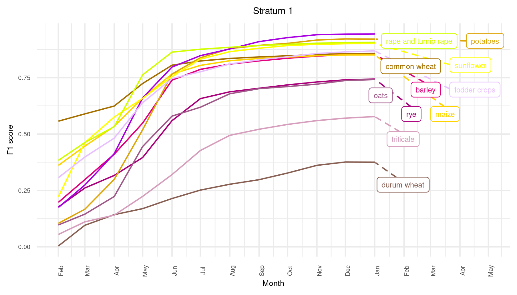
(a)

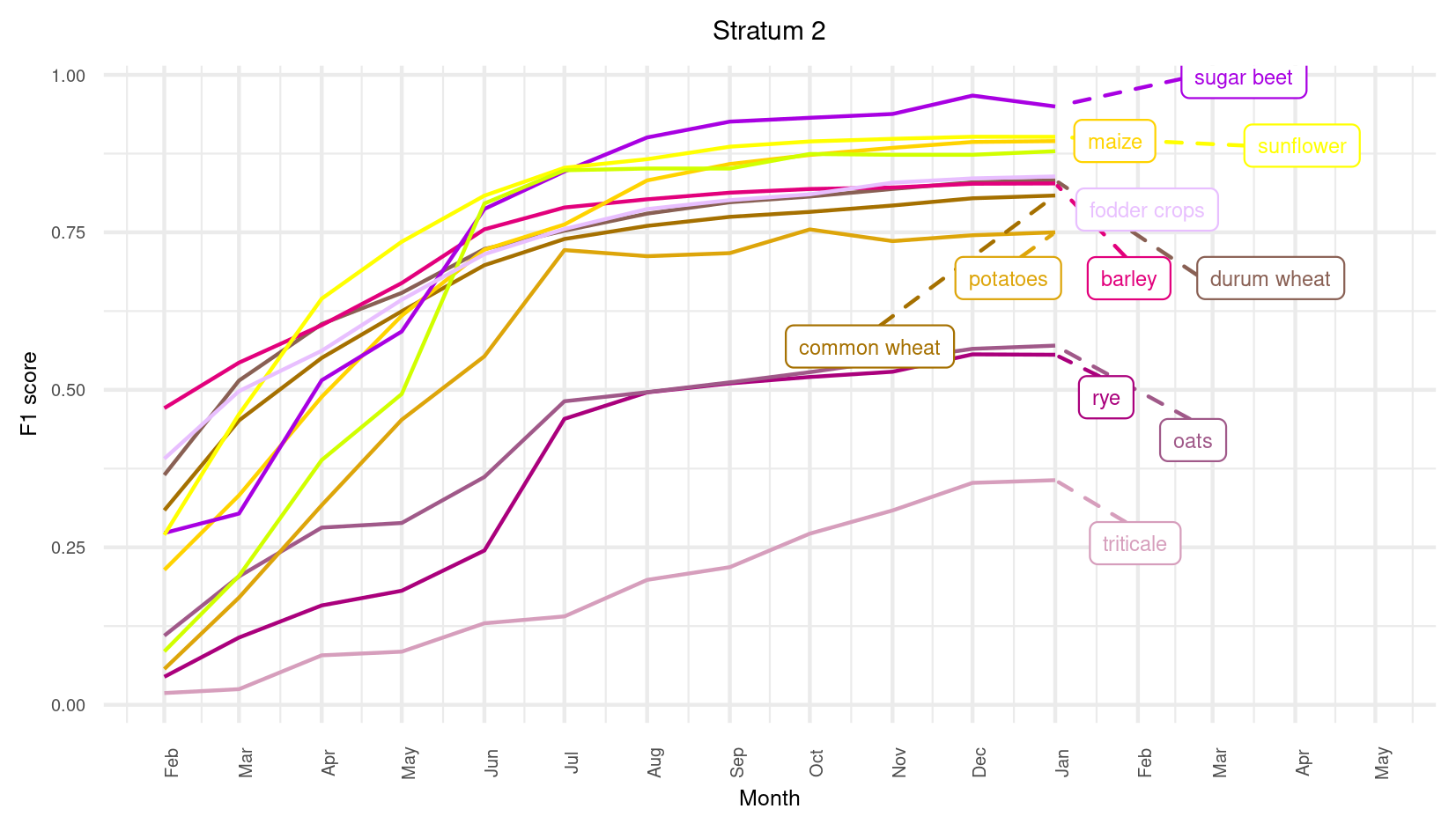
(b)

Supplementary Fig. S1: Evolution of The F-score for each Stratum through time for the 12 mains crops over the EU-28.

Supplementary Table S4: Masking the EU crop map for visualization and area estimation

	Classes labels	Class codes
Corine Land Cover 2018
	Inland and coastal wetlands	411-412, 421-423
	Moors and Heatlands	322
	Bare Lands	331-333,335
	Port and airports	123,124
JRC GHSL European Settlement Map R2019	Residential and non residential built-up area	250, 255
JRC Surface Water 2019	2019 permanent water bodies	3

Supplementary Table S5: Area (ha) of the EU crop type classes, with the projection EPSG 3035

Class	Area (ha)
211	$31,325,983.42$
212	$1,842,598.45$
213	$11,822,095.11$
214	$1,641,600.28$
215	$457,025.1$
216	$22,188,829.6$
217	$3380.94$
218	$33,631.6$
219	$13,944.24$
221	$785,300.85$
222	$1,753,491.13$
223	$19,124.88$
230	$393,616.4$
231	$4,551,610.89$
232	$6,868,240.33$
233	$62,272.83$
240	$1,731,230.9$
250	$1,872,904.25$
290	$4,375,965.4$
Total arable land	$91,742,847$
300	$223,436,295.7$
500	$70,941,202.43$

Supplementary Table S6: Confusion matrix for the EU-28 region. The values represent sample counts. UA = User’s accuracy, PA=Producer Accuracy

	Reference class (LUCAS point)
	211	212	213	214	215	216	217	218	219	221	222	223	230	231	232	233	240	250	290	300	500	total	UA	OA
211	4624	367	833	287	348	99	7	269	25	8	11	12	52	4	93	3	47	205	598	69	1369	9330	49.6	74.0
212	68	402	61	2	37	3	1	3	0	0	0	1	2	0	0	0	10	60	43	5	111	809	49.7
213	372	121	2117	112	206	47	6	38	4	3	0	10	24	3	23	0	78	164	255	49	467	4099	51.6
214	34	3	41	236	11	2	0	99	1	1	0	0	2	0	12	0	1	1	19	0	26	489	48.3
215	26	3	14	3	56	0	0	1	0	0	0	0	1	0	0	0	1	15	8	1	21	150	37.3
216	128	16	105	21	44	3464	28	16	81	124	149	38	36	45	36	120	133	169	139	98	936	5926	58.5
217	0	0	0	0	0	0	0	0	0	0	0	0	0	0	0	0	0	0	0	0	0	0
218	2	0	1	1	0	0	0	4	0	0	0	0	0	0	0	0	0	0	0	0	0	8	50.0
219	0	0	0	0	0	0	0	0	4	1	0	0	0	0	1	0	0	0	0	0	1	7	57.1
221	0	0	0	0	0	1	0	0	0	180	35	4	0	5	2	2	6	0	5	0	5	245	73.5
222	0	0	2	0	0	21	0	0	1	68	476	7	0	17	3	11	14	1	7	2	5	635	75.0
223	0	0	0	0	0	0	0	0	0	0	0	1	0	0	0	0	2	0	0	0	0	3	33.3
230	0	0	1	0	0	0	5	0	1	1	0	0	124	5	0	0	10	1	7	0	7	162	76.5
231	5	3	9	0	1	46	4	1	1	17	28	7	36	530	3	22	40	8	37	7	47	852	62.2
232	15	1	12	3	1	4	0	5	3	1	10	4	5	2	1415	1	34	11	135	8	94	1764	80.2
233	0	0	0	0	0	1	0	0	0	0	0	0	0	0	0	8	0	0	0	0	0	9	88.9
240	5	13	13	2	1	9	1	1	6	21	4	16	8	3	37	2	213	26	51	7	89	528	40.3
250	36	44	45	4	31	21	4	3	2	0	0	2	2	1	8	0	32	203	29	16	232	715	28.4
290	21	15	24	0	13	34	34	1	0	11	2	4	11	20	12	0	35	28	667	91	335	1358	49.1
300	137	93	117	26	47	179	8	18	11	10	9	2	14	14	62	9	70	275	251	31981	5082	38415	83.3
500	441	79	253	84	131	144	2	38	19	1	1	5	22	1	18	3	46	1039	163	1532	18327	22349	82.0
Total	5914	1160	3648	781	927	4075	100	497	159	447	725	113	339	650	1725	181	772	2206	2414	33866	27154
Producer ’s accuracy	78.2	34.7	58.0	30.2	6.0	85.0	0.0	0.8	2.5	40.3	65.7	0.9	36.6	81.5	82.0	4.4	27.6	9.2	27.6	94.4	67.5

Supplementary Table S7: Confusion matrix for the EU-28 region. The values represent the estimated area proportions. UA = User’s accuracy, PA=Producer Accuracy

	Reference class (LUCAS point)
Map class	211	212	213	214	215	216	217	218	219	221	222	223	230	231	232	233	240	250	290	300	500	UA	SE	OA
211	0.04	0.003	0.007	0.002	0.003	0.001	0	0.002	0	0	0	0	0	0	0.001	0	0	0.002	0.005	0.001	0.012	49.6	1	76.3
212	0	0.002	0	0	0	0	0	0	0	0	0	0	0	0	0	0	0	0	0	0	0.001	49.7	3.4
213	0.003	0.001	0.016	0.001	0.002	0	0	0	0	0	0	0	0	0	0	0	0.001	0.001	0.002	0	0.003	51.6	1.5
214	0	0	0	0.002	0	0	0	0.001	0	0	0	0	0	0	0	0	0	0	0	0	0	48.3	4.4
215	0	0	0	0	0	0	0	0	0	0	0	0	0	0	0	0	0	0	0	0	0	37.3	7.8
216	0.001	0	0.001	0	0	0.034	0	0	0.001	0.001	0.001	0	0	0	0	0.001	0.001	0.002	0.001	0.001	0.009	58.5	1.3
217	0	0	0	0	0	0	0	0	0	0	0	0	0	0	0	0	0	0	0	0	0
218	0	0	0	0	0	0	0	0	0	0	0	0	0	0	0	0	0	0	0	0	0	50	37
219	0	0	0	0	0	0	0	0	0	0	0	0	0	0	0	0	0	0	0	0	0	57.1	39.6
221	0	0	0	0	0	0	0	0	0	0.001	0	0	0	0	0	0	0	0	0	0	0	73.5	5.5
222	0	0	0	0	0	0	0	0	0	0	0.003	0	0	0	0	0	0	0	0	0	0	75	3.4
223	0	0	0	0	0	0	0	0	0	0	0	0	0	0	0	0	0	0	0	0	0	33.3	65.3
230	0	0	0	0	0	0	0	0	0	0	0	0	0.001	0	0	0	0	0	0	0	0	76.5	6.5
231	0	0	0	0	0	0.001	0	0	0	0	0	0	0	0.007	0	0	0.001	0	0.001	0	0.001	62.2	3.3
232	0	0	0	0	0	0	0	0	0	0	0	0	0	0	0.014	0	0	0	0.001	0	0.001	80.2	1.9
233	0	0	0	0	0	0	0	0	0	0	0	0	0	0	0	0	0	0	0	0	0	88.9	21.8
240	0	0	0	0	0	0	0	0	0	0	0	0	0	0	0	0	0.002	0	0	0	0.001	40.3	4.2
250	0	0	0	0	0	0	0	0	0	0	0	0	0	0	0	0	0	0.001	0	0	0.002	28.4	3.3
290	0	0	0	0	0	0	0	0	0	0	0	0	0	0	0	0	0	0	0.006	0.001	0.003	49.1	2.7
300	0.002	0.001	0.002	0	0.001	0.003	0	0	0	0	0	0	0	0	0.001	0	0.001	0.004	0.004	0.482	0.077	83.3	0.4
500	0.004	0.001	0.002	0.001	0.001	0.001	0	0	0	0	0	0	0	0	0	0	0	0.009	0.001	0.013	0.151	82	0.5
PA(%)	78	25.5	53.4	30.2	5.6	83.8	0	1	1.4	37.6	57.5	1.6	26.8	86.7	82.3	7.5	25	6.9	25	96.9	58
SE(%)	1	1.9	1.4	2.6	1.2	1.2	0	0.7	1	3.3	3.2	3.1	3.2	2.2	1.7	2	2.5	0.8	1.4	0.1	0.5

Supplementary Table S8: Confusion matrix for main crop type group for the EU-28 region. The values represent sample counts. UA = User’s accuracy, PA=Producer Accuracy

		Reference class (LUCAS point)
	Map Class	210	220	230	240	250	290	300	500	Total	UA (%)	OA(%)
210	Cereals	14904	358	240	270	614	1062	222	2931	20601	72.3	79.2
220	Root Crops	25	771	13	22	1	12	2	10	856	90.1
230	Non permanent industrial crops	8	1	132	10	1	7	0	7	166	79.5
240	Dry pulses, Vegetables and Flowers	51	41	10	213	26	51	7	89	488	43.6
250	Fodder Crops	190	2	2	32	203	29	16	232	706	28.8
290	Bare Arable Land	142	17	11	35	28	667	91	335	1326	50.3
300	Tree and Shrub Cover	636	21	23	70	275	251	31981	5082	38339	83.4
500	Grassland	1191	7	25	46	1039	163	1532	18327	22330	82.1
	Total	17147	1218	456	698	2187	2242	33851	27013
	PA (%)	86.9	63.3	28.9	30.5	9.3	29.8	94.5	67.8

Supplementary Table S9: F-score by country for the 6 main crops

Country	# points	Fscore 211	Fscore 213	Fscore 216	Fscore 222	Fscore 231	Fscore 232
AT	1750	0.63	0.54	0.70	0.46	0.50	0.96
BE	946	0.69	0.51	0.72	0.65		0.83
BG	1751	0.68	0.27	0.71		0.97	0.87
CY	487	0.32	0.15
CZ	2084	0.78	0.65	0.85	0.98		0.96
DE	9170	0.67	0.62	0.85	0.75	0.22	0.90
DK	1069	0.57	0.69	0.77	0.74		0.87
EE	666	0.46	0.57				0.70
EL	2991	0.09	0.26	0.33		0.31
ES	13242	0.53	0.60	0.42		0.46	0.51
FI	3183	0.18	0.54				0.41
FR	15024	0.74	0.57	0.72	0.80	0.78	0.87
HR	983	0.36		0.74	0.22	0.84	0.13
HU	1428	0.58	0.16	0.83	0.36	0.86	0.78
IE	1329	0.56	0.81	0.21			0.67
IT	6280	0.55	0.17	0.64	0.47	0.55	0.26
LT	1138	0.56	0.20	0.33	0.57		0.88
LU	106	0.71	0.75	0.67			1.00
LV	1313	0.67	0.28	0.12			0.88
MT	11
NL	1437	0.58	0.23	0.69	0.58
PL	7810	0.51	0.32	0.70	0.75		0.88
PT	2230	0.05	0.29	0.48
RO	3528	0.26	0.08	0.62	0.30	0.76	0.47
SE	4756	0.48	0.50	0.16	0.40		0.74
SI	634	0.55		0.81		0.67
SK	818	0.73	0.54	0.46		0.75	0.92
UK	5037	0.58	0.64	0.27	0.38		0.48

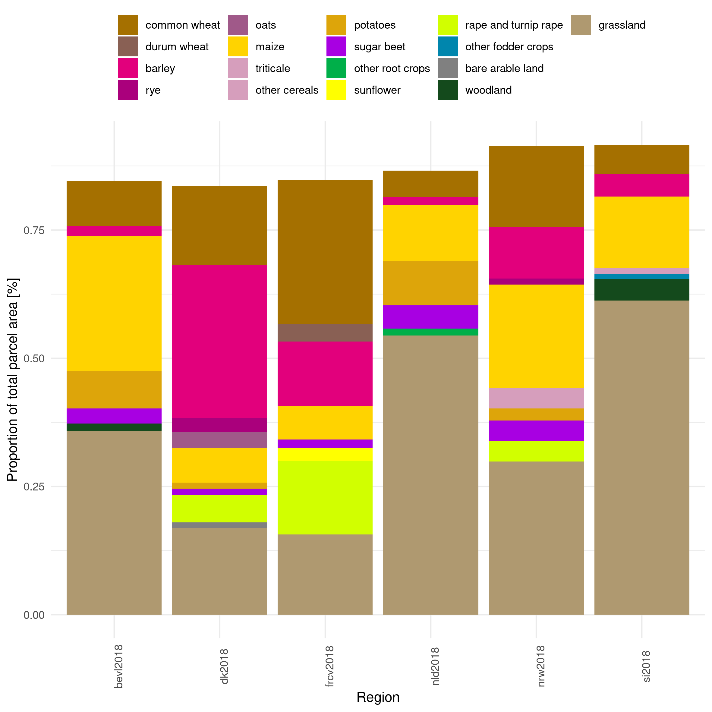
Supplementary Fig. S2: Proportion of total GSAA declared area in 2018 by crop in the six regions of interest. Crop type covering an area smaller than 1% of the total are neglected.

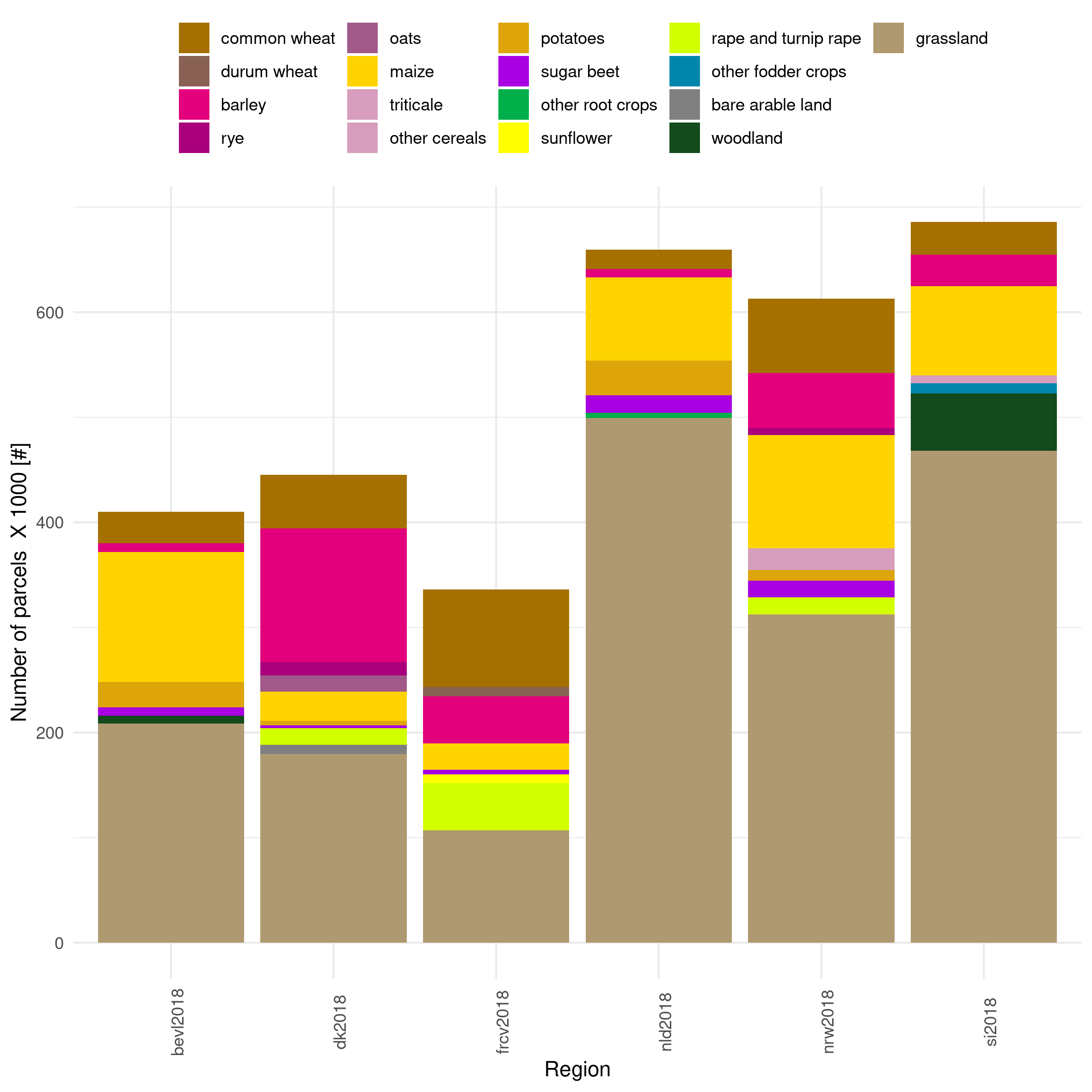
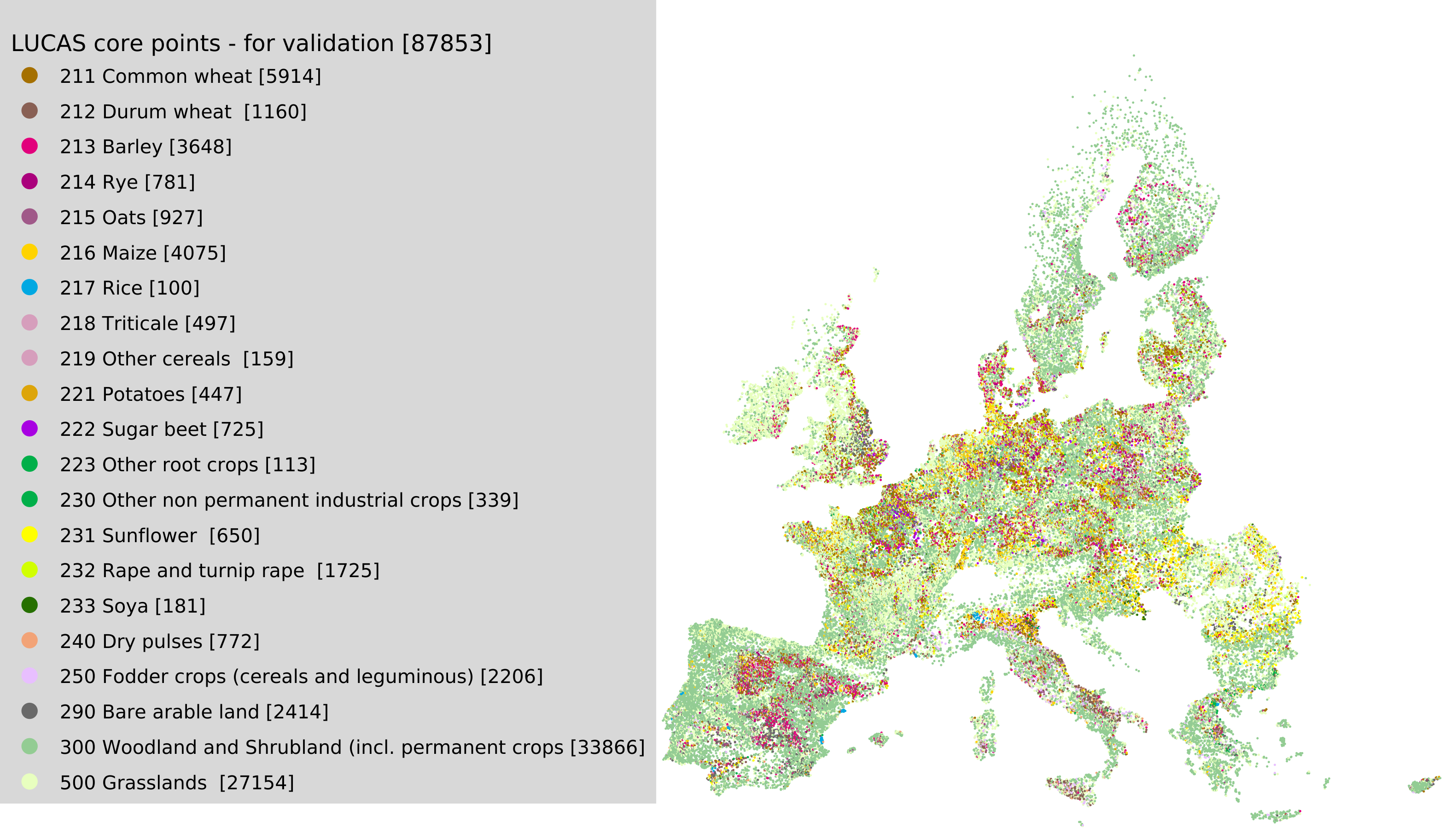
Supplementary Fig. S3: Area of total GSAA declared area in 2018 by crop in the six regions of interest. Crop type covering an area smaller than 1% of the total are neglected.

Supplementary Fig. S4: Validation points (87,853) are high-quality point of the LUCAS core survey 2018 not used for training

Supplementary Table S10: Summary of GSAA legend matching data used in the study.

Region	Crop code	211	212	213	214	215	216	218	219	221	222	223	231	232	250	290	300	500
bevl2018	hfdtlt	311	0	321	0	0	201,202	0	0	901,904	91	0	0	0	0	0	9711	60,700
dk2018	afgkode	2,11	0	1,10	15	3	216	0	0	151	160	0	0	22	0	318	0	101,252,254,260,263,276,308
frcv2018	cropcode	801	1	809	0	0	5,6	0	807	0	1	0	1	1	208	0	100,699	201,203,204
nld2018	gws_gewasc	233	0	236	0	0	259	0	0	2014,2015,2017	256	262	0	0	0	0	0	265,266,331,335,336
nrw2018	mon10_cr_1	115	0	131,132	121	0	171,411	156	0	602	603	0	0	311	0	0	0	424,459
si2018	sifra_kmrs	1	10	6,7	0	0	4,5	0	1	0	189	0	39	37	1	0	2	149,150,151

Supplementary Table S11: Confusion matrix for bevl2018

	211	213	216	221	222	TOTAL	UA
211	26456	118	262	4	6	26846	0.9855
213	1168	5401	107	0	1	6677	0.8089
216	734	196	102799	107	42	103878	0.9896
221	37	10	10086	11555	1332	23020	0.502
222	16	7	2170	982	4804	7979	0.6021
TOTAL	28411	5732	115424	12648	6185	168400
PA	0.9312	0.9423	0.8906	0.9136	0.7767

Supplementary Table S12: Confusion matrix for dk2018

	211	213	214	215	216	221	222	232	290	TOTAL	UA
211	41660	3267	56	7	167	3	0	30	0	45190	0.9219
213	4593	100065	103	11	1679	37	39	97	7	106631	0.9384
214	2423	2088	7524	0	30	1	0	4	0	12070	0.6234
215	1546	7060	14	70	386	5	0	15	3	9099	0.0077
216	213	513	3	2	25374	10	1	1	0	26117	0.9716
221	9	26	0	0	1788	2197	21	0	0	4041	0.5437
222	11	52	0	0	679	28	1929	0	0	2699	0.7147
232	135	312	4	0	66	0	1	14467	1	14986	0.9654
290	5	8	0	1	20	0	0	0	0	34	0
TOTAL	50595	113391	7704	91	30189	2281	1991	14614	11	220867
PA	0.8234	0.8825	0.9766	0.7692	0.8405	0.9632	0.9689	0.9899	0

Supplementary Table S13: Confusion matrix for si2018

	211	213	216	219	250	TOTAL	UA
211	18662	155	6689	0	31	25537	0.7308
213	8539	4118	7979	0	98	20734	0.1986
216	608	31	69898	0	13	70550	0.9908
219	3633	72	1765	0	10	5480	0
250	184	27	1373	0	23	1607	0.0143
TOTAL	31626	4403	87704	0	175	123908
PA	0.5901	0.9353	0.797	NaN	0.1314

Supplementary Table S14: Confusion matrix for frcv2018

	211	212	213	216	222	231	232	TOTAL	UA
211	88981	0	233	224	10	10	122	89580	0.9933
212	8413	0	88	31	3	0	8	8543	0
213	7186	0	34060	636	13	9	75	41979	0.8114
216	217	0	49	21902	10	11	54	22243	0.9847
222	25	0	7	173	3723	51	33	4012	0.928
231	59	0	9	1317	74	6768	25	8252	0.8202
232	124	0	24	49	1	11	43836	44045	0.9953
TOTAL	105005	0	34470	24332	3834	6860	44153	218654
PA	0.8474	-	0.9881	0.9001	0.971	0.9866	0.9928

Supplementary Table S15: Confusion matrix for nld2018

	211	213	216	221	222	223	TOTAL	UA
211	17352	148	178	6	4	0	17688	0.981
213	1873	4224	473	4	3	1	6578	0.6421
216	564	420	73207	57	14	16	74278	0.9856
221	71	38	7823	20472	3565	9	31978	0.6402
222	32	25	5229	969	10416	7	16678	0.6245
223	306	311	2674	10	108	1210	4619	0.262
TOTAL	20198	5166	89584	21518	14110	1243	151819
PA	0.8591	0.8177	0.8172	0.9514	0.7382	0.9735

Supplementary Table S16: Confusion matrix for nrw2018

	211	213	214	216	218	221	222	232	TOTAL	UA
211	69259	274	164	268	0	4	15	45	70029	0.989
213	10833	37528	220	556	0	1	7	125	49270	0.7617
214	1455	754	3918	48	0	1	1	17	6194	0.6325
216	824	135	43	102231	0	17	23	61	103334	0.9893
218	12692	2064	4921	92	8	2	0	42	19821	4e-04
221	96	15	2	2204	0	4365	2564	29	9275	0.4706
222	41	13	0	2039	0	231	13238	5	15567	0.8504
232	94	17	0	28	0	0	0	16175	16314	0.9915
TOTAL	95294	40800	9268	107466	8	4621	15848	16499	289804
PA	0.7268	0.9198	0.4227	0.9513	1	0.9446	0.8353	0.9804

Supplementary Table S17: Legend convergence between Eurostat and EU crop map classes

estat_crop_class	estat_crop_label	eucropmap_class	eucropmap_label
C1110	Common wheat and spelt	211	common wheat
C1120	Durum wheat	212	durum wheat
C1200	Rye and winter cereal mixtures (maslin)	214	rye
C1300	Barley	213	barley
C1410	Oats	215	oats
C1500	Grain maize and corn-cob-mix	216	maize
C1600	Triticale	218	triticale
C2000	Rice	217	rice
G3000	Green maize	216	maize
R1000	Potatoes (including seed potatoes)	221	potatoes
R2000	Sugar beet (excluding seed)	222	sugar beet
I1110	Rape and turnip rape seeds	232	rape and turnip rape
I1120	Sunflower seed	231	sunflower
I1130	Soya	233	soya

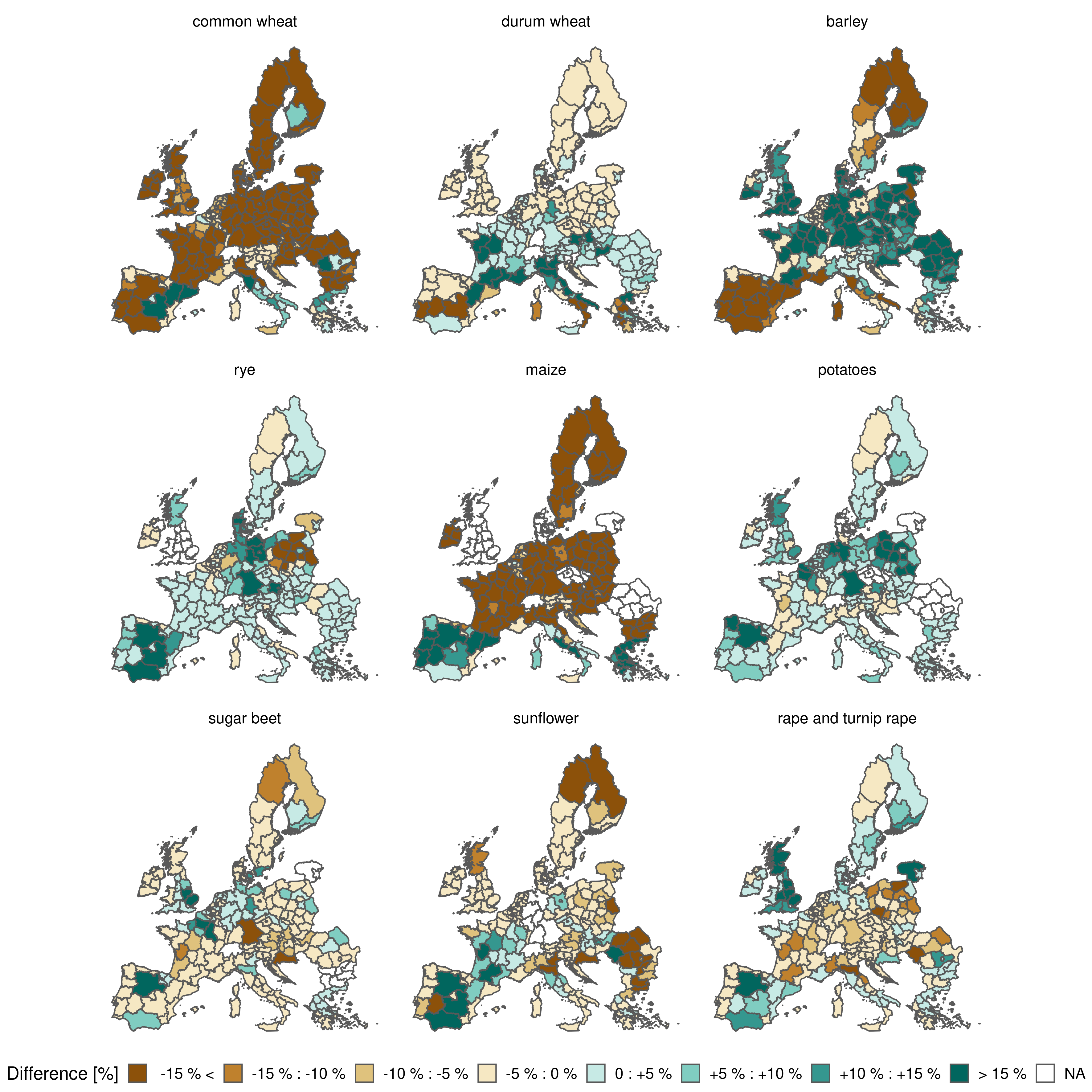
Supplementary Fig. S5: Relative difference of area [%] reported by Eurostat and retrieved from the EU crop map. The difference is the Eurostat reported value minus the value estimated from the EU crop map. Green values means that the EU crop map underestimates the area compared to the data reported from Eurostat while the brown values means that there is an overestimation.

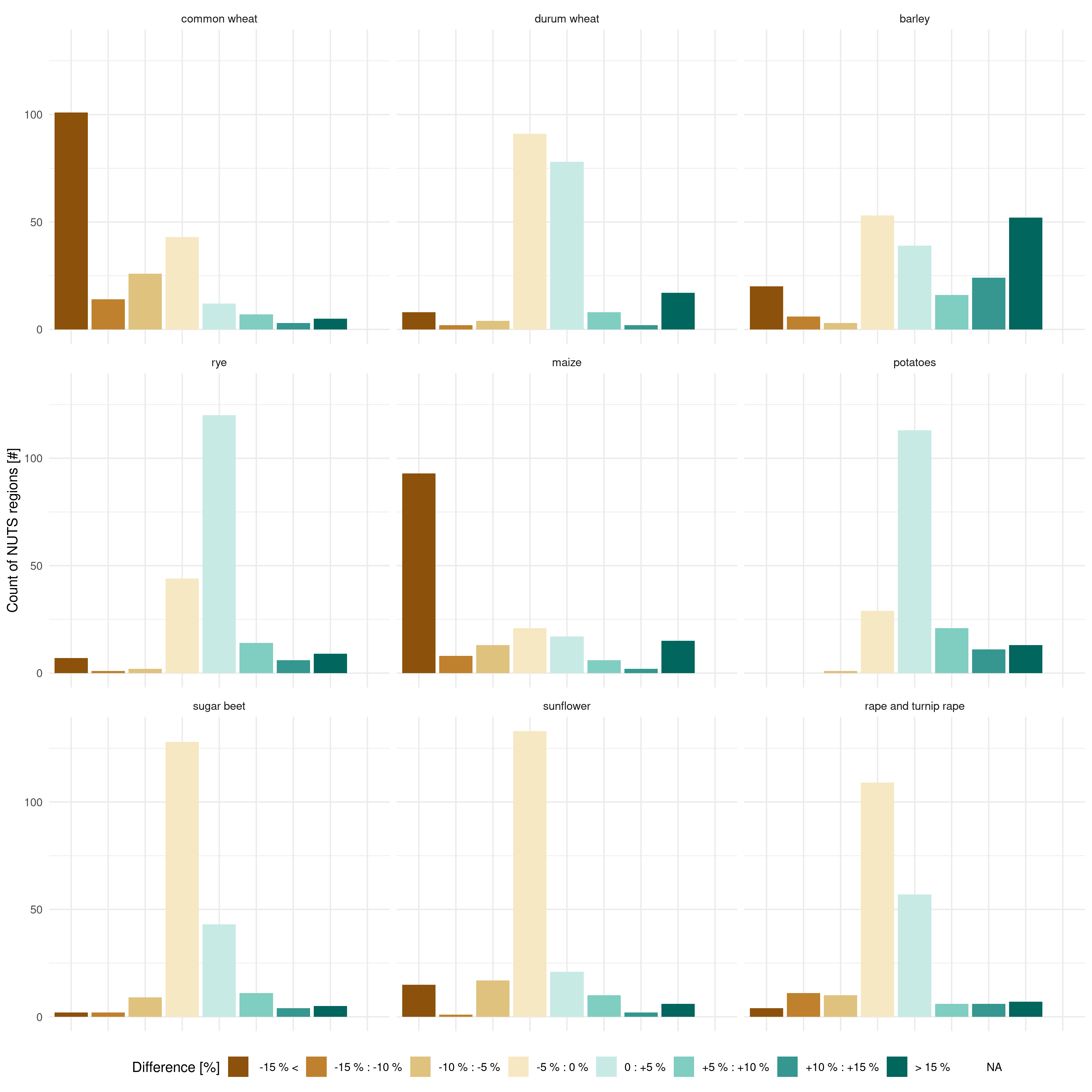
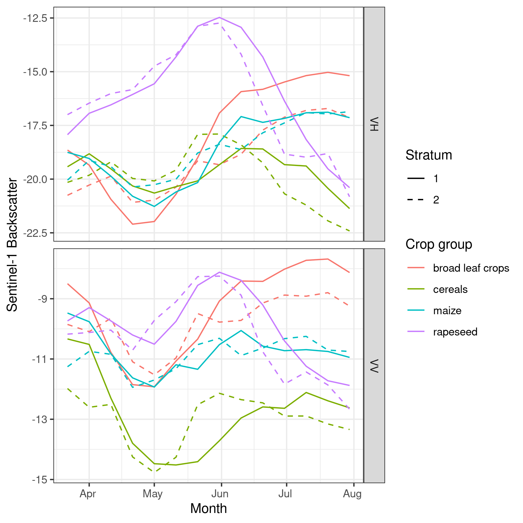
Supplementary Fig. S6: The areas reported by Eurostat at NUTS2 level (except for UK and DE at NUTS1) are compared with the area retrieved from the EUcropmap. The difference is the Eurostat reported value minus the value estimated from the EU crop map. Green values means that the EU crop map underestimates the area compared to the data reported from Eurostat while the brown values means that there is an overestimation.

Supplementary Fig. S7: Sentinel-1 backscattering coefficient VV and VH are grouped for broad leaf crops (potato, sugar beet, sunflower), cereals (common wheat, durum wheat, barley, rye, oats, triticale), maize and rapeseed. This grouping better illustrates the differences observed in the north (stratum 1) and in the south (stratum 2).

References

- Belgiu & Csillik [2018] Belgiu, M., & Csillik, O. (2018). Sentinel-2 cropland mapping using pixel-based and object-based time-weighted dynamic time warping analysis. Remote sensing of environment, 204, 509–523.
- Belgiu & Drăguţ [2016] Belgiu, M., & Drăguţ, L. (2016). Random forest in remote sensing: A review of applications and future directions. ISPRS Journal of Photogrammetry and Remote Sensing, 114, 24–31.
- Breiman [2001] Breiman, L. (2001). Random forests. Machine learning, 45, 5–32.
- Buras et al. [2019] Buras, A., Rammig, A., & Zang, C. S. (2019). Quantifying impacts of the drought 2018 on european ecosystems in comparison to 2003. arXiv preprint arXiv:1906.08605, .
- Chakhar et al. [2021] Chakhar, A., Hernández-López, D., Ballesteros, R., & Moreno, M. A. (2021). Improving the accuracy of multiple algorithms for crop classification by integrating sentinel-1 observations with sentinel-2 data. Remote Sensing, 13, 243.
- Clauss et al. [2018] Clauss, K., Ottinger, M., & Künzer, C. (2018). Mapping rice areas with sentinel-1 time series and superpixel segmentation. International Journal of Remote Sensing, 39, 1399–1420.
- Close et al. [2018] Close, O., Benjamin, B., Petit, S., Fripiat, X., & Hallot, E. (2018). Use of Sentinel-2 and LUCAS Database for the Inventory of Land Use, Land Use Change, and Forestry in Wallonia, Belgium. Land, 7, 154. URL: http://www.mdpi.com/2073-445X/7/4/154. doi:10.3390/land7040154.
- Corbane et al. [2020] Corbane, C., Sabo, F., Syrris, V., Kemper, T., Politis, P., Pesaresi, M., Soille, P., & Osé, K. (2020). Application of the symbolic machine learning to copernicus vhr imagery: The european settlement map. IEEE Geoscience and Remote Sensing Letters, 17, 1153–1157. doi:10.1109/LGRS.2019.2942131.
- d’Andrimont et al. [2018a] d’Andrimont, R., Lemoine, G., & Van der Velde, M. (2018a). Targeted grassland monitoring at parcel level using sentinels, street-level images and field observations. Remote Sensing, 10, 1300.
- d’Andrimont et al. [2020a] d’Andrimont, R., Taymans, M., Lemoine, G., Ceglar, A., Yordanov, M., & van der Velde, M. (2020a). Detecting flowering phenology in oil seed rape parcels with sentinel-1 and-2 time series. Remote sensing of environment, 239, 111660.
- d’Andrimont et al. [2021] d’Andrimont, R., Verhegghen, A., Meroni, M., Lemoine, G., Strobl, P., Eiselt, B., Yordanov, M., Martinez-Sanchez, L., & van der Velde, M. (2021). Lucas copernicus 2018: Earth-observation-relevant in situ data on land cover and use throughout the european union. Earth System Science Data, 13, 1119–1133.
- d’Andrimont et al. [2018b] d’Andrimont, R., Yordanov, M., Lemoine, G., Yoong, J., Nikel, K., & van der Velde, M. (2018b). Crowdsourced street-level imagery as a potential source of in-situ data for crop monitoring. Land, 7, 127.
- d’Andrimont et al. [2020b] d’Andrimont, R., Yordanov, M., Martinez-Sanchez, L., Eiselt, B., Palmieri, A., Dominici, P., Gallego, J., Reuter, H. I., Joebges, C., Lemoine, G. et al. (2020b). Harmonised lucas in-situ land cover and use database for field surveys from 2006 to 2018 in the european union. Scientific Data, 7, 1–15.
- De Vroey et al. [2021] De Vroey, M., Radoux, J., & Defourny, P. (2021). Grassland mowing detection using sentinel-1 time series: Potential and limitations. Remote Sensing, 13, 348.
- Defourny et al. [2019] Defourny, P., Bontemps, S., Bellemans, N., Cara, C., Dedieu, G., Guzzonato, E., Hagolle, O., Inglada, J., Nicola, L., Rabaute, T. et al. (2019). Near real-time agriculture monitoring at national scale at parcel resolution: Performance assessment of the sen2-agri automated system in various cropping systems around the world. Remote Sensing of Environment, 221, 551–568.
- Dinerstein et al. [2017] Dinerstein, E., Olson, D., Joshi, A., Vynne, C., Burgess, N. D., Wikramanayake, E., Hahn, N., Palminteri, S., Hedao, P., Noss, R. et al. (2017). An ecoregion-based approach to protecting half the terrestrial realm. BioScience, 67, 534–545.
- Dobson & Ulaby [1981] Dobson, M. C., & Ulaby, F. (1981). Microwave backscatter dependence on surface roughness, soil moisture, and soil texture: Part iii-soil tension. IEEE Transactions on Geoscience and Remote Sensing, (pp. 51–61).
- EEA [2018] EEA (2018). Corine land cover (clc) 2018, version 20b2. Release Date: 21-12-2018, .
- European Commission [2019] European Commission (2019). Agri-food trade in 2018: another successful year for agri-food trade. https://ec.europa.eu/info/sites/info/files/food-farming-fisheries/news/documents/agri-food-trade-2018_en.pdf. (Accessed on 03/16/2021).
- Eurostat [2018a] Eurostat (2018a). Lucas web site. https://ec.europa.eu/eurostat/web/lucas. (Accessed on 08/30/2018).
- Eurostat [2018b] Eurostat (2018b). Technical reference document c-1: Instructions for surveyors. https://ec.europa.eu/eurostat/documents/205002/8072634/LUCAS2018-C1-Instructions.pdf. (Accessed on 07/30/2019).
- Eurostat [2018c] Eurostat (2018c). Technical reference document c-3: Classification. https://ec.europa.eu/eurostat/documents/205002/8072634/LUCAS2018-C3-Classification.pdf. (Accessed on 07/30/2019).
- Gallego [2004] Gallego, F. J. (2004). Remote sensing and land cover area estimation. International Journal of Remote Sensing, 25, 3019–3047.
- Gallego & Bamps [2008] Gallego, J., & Bamps, C. (2008). Using corine land cover and the point survey lucas for area estimation. International Journal of Applied Earth Observation and Geoinformation, 10, 467–475.
- Gallego & Delincé [2010] Gallego, J., & Delincé, J. (2010). The european land use and cover area-frame statistical survey. Agricultural survey methods, (pp. 149–168).
- Gao et al. [2018] Gao, H., Wang, C., Wang, G., Zhu, J., Tang, Y., Shen, P., & Zhu, Z. (2018). A crop classification method integrating gf-3 polsar and sentinel-2a optical data in the dongting lake basin. Sensors, 18, 3139.
- Gorelick et al. [2017] Gorelick, N., Hancher, M., Dixon, M., Ilyushchenko, S., Thau, D., & Moore, R. (2017). Google earth engine: Planetary-scale geospatial analysis for everyone. Remote Sensing of Environment, .
- Immitzer et al. [2016] Immitzer, M., Vuolo, F., & Atzberger, C. (2016). First experience with sentinel-2 data for crop and tree species classifications in central europe. Remote Sensing, 8, 166.
- Inglada et al. [2017] Inglada, J., Vincent, A., Arias, M., Tardy, B., Morin, D., & Rodes, I. (2017). Operational high resolution land cover map production at the country scale using satellite image time series. Remote Sensing, 9, 95.
- Joly et al. [2016] Joly, A., Bonnet, P., Goëau, H., Barbe, J., Selmi, S., Champ, J., Dufour-Kowalski, S., Affouard, A., Carré, J., Molino, J.-F. et al. (2016). A look inside the pl@ ntnet experience. Multimedia Systems, 22, 751–766.
- Kenduiywo et al. [2018] Kenduiywo, B. K., Bargiel, D., & Soergel, U. (2018). Crop-type mapping from a sequence of sentinel 1 images. International Journal of Remote Sensing, 39, 6383–6404.
- Kussul et al. [2017] Kussul, N., Lavreniuk, M., Skakun, S., & Shelestov, A. (2017). Deep learning classification of land cover and crop types using remote sensing data. IEEE Geoscience and Remote Sensing Letters, 14, 778–782.
- Kussul et al. [2018] Kussul, N., Mykola, L., Shelestov, A., & Skakun, S. (2018). Crop inventory at regional scale in ukraine: developing in season and end of season crop maps with multi-temporal optical and sar satellite imagery. European Journal of Remote Sensing, 51, 627–636.
- Laso Bayas et al. [2020] Laso Bayas, J. C., See, L., Bartl, H., Sturn, T., Karner, M., Fraisl, D., Moorthy, I., Busch, M., van der Velde, M., & Fritz, S. (2020). Crowdsourcing lucas: Citizens generating reference land cover and land use data with a mobile app. Land, 9, 446.
- Lemoine [2017] Lemoine, G. (2017). Data access and data analysis software.. (1st ed.). Rome: Handbook on Remote Sensing for Agricultural Statistics (Chapter 1). Handbook of the Global Strategy to improve Agricultural and Rural Statistics (GSARS). doi:10.13140/RG.2.2.13259.69920.
- Lemoine et al. [2019] Lemoine, G., Devos, W., Milenov, P., & d’Andrimont, R. (2019). Machine learning for crop type identification using country-wide, consistent sentinel-1 time series. In Proc. 2019 Conference on Big Data from Space (BiDS ’19) (pp. 81–74).
- Mack et al. [2017] Mack, B., Leinenkugel, P., Kuenzer, C., & Dech, S. (2017). A semi-automated approach for the generation of a new land use and land cover product for germany based on landsat time-series and lucas in-situ data. Remote Sensing Letters, 8, 244–253.
- Massey et al. [2018] Massey, R., Sankey, T. T., Yadav, K., Congalton, R. G., & Tilton, J. C. (2018). Integrating cloud-based workflows in continental-scale cropland extent classification. Remote Sensing of Environment, 219, 162–179.
- McNairn & Brisco [2004] McNairn, H., & Brisco, B. (2004). The application of c-band polarimetric sar for agriculture: A review. Canadian Journal of Remote Sensing, 30, 525–542.
- Merlos & Hijmans [2020] Merlos, F. A., & Hijmans, R. J. (2020). The scale dependency of spatial crop species diversity and its relation to temporal diversity. Proceedings of the National Academy of Sciences, 117, 26176–26182.
- Meroni et al. [2021] Meroni, M., d’Andrimont, R., Vrieling, A., Fasbender, D., Lemoine, G., Rembold, F., Seguini, L., & Verhegghen, A. (2021). Comparing land surface phenology of major european crops as derived from sar and multispectral data of sentinel-1 and-2. Remote sensing of environment, 253, 112232.
- Ndikumana et al. [2018] Ndikumana, E., Ho Tong Minh, D., Baghdadi, N., Courault, D., & Hossard, L. (2018). Deep recurrent neural network for agricultural classification using multitemporal sar sentinel-1 for camargue, france. Remote Sensing, 10, 1217.
- Olofsson et al. [2014] Olofsson, P., Foody, G. M., Herold, M., Stehman, S. V., Woodcock, C. E., & Wulder, M. A. (2014). Good practices for estimating area and assessing accuracy of land change. Remote Sensing of Environment, 148, 42–57. URL: http://www.sciencedirect.com/science/article/pii/S0034425714000704http://dx.doi.org/10.1016/j.rse.2014.02.015. doi:10.1016/j.rse.2014.02.015.
- Orynbaikyzy et al. [2020] Orynbaikyzy, A., Gessner, U., Mack, B., & Conrad, C. (2020). Crop type classification using fusion of sentinel-1 and sentinel-2 data: Assessing the impact of feature selection, optical data availability, and parcel sizes on the accuracies. Remote Sensing, 12, 2779.
- Pedregosa et al. [2011] Pedregosa, F., Varoquaux, G., Gramfort, A., Michel, V., Thirion, B., Grisel, O., Blondel, M., Prettenhofer, P., Weiss, R., Dubourg, V., Vanderplas, J., Passos, A., Cournapeau, D., Brucher, M., Perrot, M., & Duchesnay, E. (2011). Scikit-learn: Machine learning in Python. Journal of Machine Learning Research, 12, 2825–2830.
- Pekel et al. [2016] Pekel, J.-F., Cottam, A., Gorelick, N., & Belward, A. S. (2016). High-resolution mapping of global surface water and its long-term changes. Nature, 540, 418–422. URL: http://www.nature.com/articles/nature20584. doi:10.1038/nature20584.
- Pelletier et al. [2016] Pelletier, C., Valero, S., Inglada, J., Champion, N., & Dedieu, G. (2016). Assessing the robustness of random forests to map land cover with high resolution satellite image time series over large areas. Remote Sensing of Environment, 187, 156–168.
- Pflugmacher et al. [2019] Pflugmacher, D., Rabe, A., Peters, M., & Hostert, P. (2019). Mapping pan-european land cover using landsat spectral-temporal metrics and the european lucas survey. Remote Sensing of Environment, 221, 583–595.
- Sabo et al. [2019] Sabo, F., Corbane, C., Politis, P., Pesaresi, M., & Kemper, T. (2019). Update and improvement of the european settlement map. In 2019 Joint Urban Remote Sensing Event (JURSE) (pp. 1–4). doi:10.1109/JURSE.2019.8808933.
- Scarno et al. [2018] Scarno, M., Ballin, M., Barcaroli, G., & Masselli, M. (2018). Redesign sample for Land Use/Cover Area frame Survey (LUCAS) 2018. Statistical Working Papers, . doi:10.2785/132365.
- Small [2011] Small, D. (2011). Flattening gamma: Radiometric terrain correction for sar imagery. IEEE Transactions on Geoscience and Remote Sensing, 49, 3081–3093.
- Soille et al. [2018] Soille, P., Burger, A., De Marchi, D., Kempeneers, P., Rodriguez, D., Syrris, V., & Vasilev, V. (2018). A versatile data-intensive computing platform for information retrieval from big geospatial data. Future Generation Computer Systems, 81, 30–40. URL: https://doi.org/10.1016/j.future.2017.11.007. doi:10.1016/j.future.2017.11.007.
- Stehman [2014] Stehman, S. V. (2014). Estimating area and map accuracy for stratified random sampling when the strata are different from the map classes. International Journal of Remote Sensing, 35, 4923–4939. URL: http://dx.doi.org/10.1080/01431161.2014.930207. doi:10.1080/01431161.2014.930207.
- Tamm et al. [2016] Tamm, T., Zalite, K., Voormansik, K., & Talgre, L. (2016). Relating sentinel-1 interferometric coherence to mowing events on grasslands. Remote Sensing, 8, 802.
- Teluguntla et al. [2018] Teluguntla, P., Thenkabail, P., Oliphant, A., Xiong, J., Gumma, M. K., Congalton, R. G., Yadav, K., & Huete, A. (2018). A 30-m landsat-derived cropland extent product of australia and china using random forest machine learning algorithm on google earth engine cloud computing platform. ISPRS journal of photogrammetry and remote sensing, 144, 325–340.
- Tian et al. [2021] Tian, F., Cai, Z., Jin, H., Hufkens, K., Scheifinger, H., Tagesson, T., Smets, B., Van Hoolst, R., Bonte, K., Ivits, E. et al. (2021). Calibrating vegetation phenology from sentinel-2 using eddy covariance, phenocam, and pep725 networks across europe. Remote Sensing of Environment, 260, 112456.
- Toreti et al. [2019] Toreti, A., Belward, A., Perez-Dominguez, I., Naumann, G., Luterbacher, J., Cronie, O., Seguini, L., Manfron, G., Lopez Lozano, R., Baruth, B. et al. (2019). The exceptional 2018 european water seesaw calls for action on adaptation. Earth’s Future, .
- Toth & Milenov [2020] Toth, K., & Milenov, P. (2020). Technical guidelines on iacs spatial data sharing. part 1, data discovery - publications office of the eu. EUR 30330 EN, .
- Ulaby et al. [1981] Ulaby, F. T., Moore, R. K., & Fung, A. K. (1981). Microwave remote sensing: Active and passive. volume 1-microwave remote sensing fundamentals and radiometry. .
- Van Horn et al. [2018] Van Horn, G., Mac Aodha, O., Song, Y., Cui, Y., Sun, C., Shepard, A., Adam, H., Perona, P., & Belongie, S. (2018). The inaturalist species classification and detection dataset. In Proceedings of the IEEE conference on computer vision and pattern recognition (pp. 8769–8778).
- Van Tricht et al. [2018] Van Tricht, K., Gobin, A., Gilliams, S., & Piccard, I. (2018). Synergistic use of radar sentinel-1 and optical sentinel-2 imagery for crop mapping: a case study for belgium. Remote Sensing, 10, 1642.
- van der Velde et al. [2019] van der Velde, M., van Diepen, C., & Baruth, B. (2019). The european crop monitoring and yield forecasting system: Celebrating 25 years of jrc mars bulletins. Agricultural Systems, 168, 56–57.
- Veloso et al. [2017] Veloso, A., Mermoz, S., Bouvet, A., Le Toan, T., Planells, M., Dejoux, J.-F., & Ceschia, E. (2017). Understanding the temporal behavior of crops using sentinel-1 and sentinel-2-like data for agricultural applications. Remote sensing of environment, 199, 415–426.
- Wang et al. [2019] Wang, S., Azzari, G., & Lobell, D. B. (2019). Crop type mapping without field-level labels: Random forest transfer and unsupervised clustering techniques. Remote Sensing of Environment, 222, 303–317. doi:10.1016/j.rse.2018.12.026.
- Wei et al. [2019] Wei, S., Zhang, H., Wang, C., Wang, Y., & Xu, L. (2019). Multi-temporal sar data large-scale crop mapping based on u-net model. Remote Sensing, 11, 68.
- Weigand et al. [2020] Weigand, M., Staab, J., Wurm, M., & Taubenböck, H. (2020). Spatial and semantic effects of lucas samples on fully automated land use/land cover classification in high-resolution sentinel-2 data. International Journal of Applied Earth Observation and Geoinformation, 88, 102065.
- You & Dong [2020] You, N., & Dong, J. (2020). Examining earliest identifiable timing of crops using all available sentinel 1/2 imagery and google earth engine. ISPRS Journal of Photogrammetry and Remote Sensing, 161, 109–123.