SDP-based bounds for graph partition via extended ADMM††thanks: This project has received funding from the European Union’s Horizon 2020 research and innovation programme under the Marie Skłodowska-Curie grant agreement MINOA No 764759.
Abstract
We study two NP-complete graph partition problems, -equipartition problems and graph partition problems with knapsack constraints (GPKC). We introduce tight SDP relaxations with nonnegativity constraints to get lower bounds, the SDP relaxations are solved by an extended alternating direction method of multipliers (ADMM). In this way, we obtain high quality lower bounds for -equipartition on large instances up to vertices within as few as five minutes and for GPKC problems up to vertices within as little as one hour. On the other hand, interior point methods fail to solve instances from due to memory requirements. We also design heuristics to generate upper bounds from the SDP solutions, giving us tighter upper bounds than other methods proposed in the literature with low computational expense.
keywords:
Graph partitioning, Semidefinite programming, ADMM, Combinatorial optimization1 Introduction
Graph partition problems have gained importance recently due to their applications in the area of engineering and computer science such as telecommunication [16] and parallel computing [12]. The solution of a graph partition problem would serve to partition the vertices of a graph into several groups under certain constraints for capacity or cardinality in each group. The optimal solution is expected to have the smallest total weight of cut edges. This problem is NP-complete [8]. Previous studies worked on improving quadratic programming or linear programming formulations to reduce the computational expense with commercial solvers [6]. Relaxations are also used to approximate this problem. Garey et al. [8] were the first to use eigenvalue and eigenvector information to get relaxations for graph partition. Ghaddar et al. [9] have recently used a branch-and-cut algorithm based on SDP relaxations to compute global optimal solutions of -partition problems.
The -equipartition problem, which is to find a partition with the minimal total weight of cut edges and the vertex set is equally partitioned into groups, is one of the most popular graph partition problems. Another problem that interests us is the graph partition problem under knapsack constraints (GPKC). In the GPKC, each vertex of the graph network is assigned a weight and the knapsack constraint needs to be satisfied in each group.
Lisser and Rendl [16] compared various semidefinite programming (SDP) relaxations and linear programming (LP) relaxations for -equipartition problems. They showed that the nonnegativity constraints become dominating in the SDP relaxation when increases. However, the application of this formulation is limited by the computing power of SDP solvers, because adding all the sign constraints for a symmetric matrix of dimension causes new constraints and entails a huge computational burden especially for large instances. Nguyen [19] proposed a tight LP relaxation for GPKC problems and a heuristic to build upper bounds as well. Semidefinite programming has shown advantages in generating tight lower bounds for quadratic problems with knapsack constraints [11] and -equipartition problem, but so far there have been no attempts to apply SDP relaxations to GPKC.
Algorithms for solving SDPs have been intensively studied in the previous years. Malick et al. [18] designed the boundary point method to solve SDP problems with equations. It can solve instances with a huge number of constraints that interior point methods (IPMs) fail to solve. This method falls into the class of alternating direction method of multipliers (ADMM). ADMM has been studied in the area of convex optimization and been proved of linear convergence when one of the objective terms is strongly convex [20]. In recent years, there have been studies focusing on generalizing this idea on solving convex optimizations with more blocks of variables. Chen et al. [3], for example, have proved the convergence of 3-block ADMM on certain scenarios, but the question as to whether the direct extension 3-block ADMM on SDP problems is convergent is still open.
There have also been varied ideas about combining other approaches with ADMM for solving SDP problems. De Santis et al. [4] added the dual factorization in the ADMM update scheme, while Sun et al. [23] combined ADMM with Newton’s methods. Both attempts have improved the performance of the algorithms.
Main results and outline
In this paper, we will introduce an extended ADMM algorithm and apply it to the tight SDP relaxations for graph partition problems with nonnegativity constraints. We will also introduce heuristics to obtain a feasible partition from the solution of the SDP relaxation.
This paper is structured as follows. In Section 2, we will introduce two graph partition problems, the -equipartition problem and the graph partition problems with knapsack constraints (GPKC). We will discuss different SDP relaxations for both problems. In Section 3, we will design an extended ADMM and illustrate its advantages in solving large SDP problems with nonnegativity constraints. In Section 4, we will introduce two post-processing methods used to generate lower bounds using the output from the extended ADMM. In Section 5, we will design heuristics to build a tight upper bound from the SDP solution to address the original problem. Numerical results of experiments carried out on graphs with different sizes and densities will be presented in Section 6. Section 7 concludes the paper.
Notation
We define by the vector of all ones of length , by the vector of all zeros of length and by the square matrix of all zeros of dimension . We omit the subscript in case the dimension is clear from the context. The notation stands for the set of integers . Let denote the set of all real symmetric matrices. We denote by that the matrix is positive semidefinite and let be the set of all positive semidefinite matrices of order . We denote by the trace inner product. That is, for any , we define . Its associated norm is the Frobenius norm, denoted by . We denote by the operation of getting the diagonal entries of matrix as a vector. The projection on the cone of positive semidefinite matrices is denoted by . The projection onto the interval is denoted by . We denote by the eigenvalues. That is, for any , we define the set of all eigenvalues of . Also, we denote the largest eigenvalue. We denote by a variable from uniform distribution between 0 and 1. We define by the index set of the largest elements.
2 Graph partition problems
2.1 -equipartition problem
For a graph , the -equipartition problem is the problem of finding an equipartition of the vertices in with groups that has the minimal total weight of edges cut by this partition. The problem can be described with binary variables,
| (1) | ||||
| s.t. | ||||
where is the Laplacian matrix for , variable indicates which group each vertex is assigned to and (resp. ) is the all-one vector of dimension (resp. ).
This problem is NP-hard and Lisser and Rendl [16] proposed the SDP relaxation
| (2) | ||||
| s.t. | ||||
where , and is the all-one vector.
To tighten this SDP relaxation, we can add more inequalities to problem (2). Here, we introduce two common inequalities for SDP relaxations derived from problems.
The process of relaxing to implies that is a nonnegative matrix, hence the first group of inequalities we consider is and the corresponding new SDP relaxation is
| (3) | ||||
| s.t. | ||||
This kind of SDP is also called a doubly nonnegative program (DNN) since the matrix variable is both, positive semidefinite and elementwise nonnegative.
Another observation is the following. For any vertices triple , if vertices and are in the same group, and vertices and are in the same group, then vertices and must be in the same group. This can be modeled by the transitivity constraints [16] given as follows
The set formed by these inequalities is the so-called metric polytop. Adding the transitivity constraints to the SDP relaxation (3) gives
| (4) | ||||
| s.t. | ||||
2.2 Graph partition problem under knapsack constraints (GPKC)
Given a graph with nonnegative weights on the vertices and a capacity bound , the GPKC asks to partition the vertices such that the total weight of cut edges is minimized and the total weight of vertices in each group does not exceed the capacity bound .
A mathematical programming formulation is given as
| (5) | ||||
| s.t. | ||||
where , is the vertex weight vector and is the capacity bound. We assume , otherwise the problem is infeasible. Again, we can derive the SDP relaxation
| (6) | ||||
| s.t. | ||||
Similar as the -equipartition problem, we can tighten the relaxation by imposing sign constraints, i.e.,
| (7) | ||||
| s.t. | ||||
and additionally by imposing the transitivity constraints which gives
| (8) | ||||
| s.t. | ||||
3 Extended ADMM
The SDP relaxations introduced in Section 2 have a huge number of constraints, even for medium-sized graphs. The total number of sign constraints for is and adding the constraint in the SDP relaxations causes extra constraints. Therefore, solving these tight relaxations is out of reach for state-of-the-art algorithms like interior point methods (IPMs). However, finding high quality lower bounds by tight SDP relaxations for graph partition problems motivates us to develop an efficient algorithm that can deal with SDP problems with inequalities and sign constraints on large-scale instances. Since the 2-block alternating direction method of multiplier (ADMM) has shown efficiency in solving large-scale instances that interior point methods fail to solve, we are encouraged to extend this algorithm for SDP problems with inequalities in the form
| (9) | ||||
| s.t. | ||||
where , , , , . We have the slack variable to form the inequality constraints, and and can be set to and respectively. Also, and can be symmetric matrices filled with all elements as and respectively. That makes formulation (9) able to represent SDP problems with any equality and inequality constraints. This formulation is inspired by the work of Sun et al. [23]. All semidefinite programs given above fit into this formulation. E.g., in (3) operator includes the diagonal-constraint and the constraint , the operator as well as the variables are not present, is the matrix of all zeros and the matrix having everywhere.
Following the ideas for the 2-block ADMM [18], we form the update scheme in Algorithm 1 to solve the dual of problem (9).
Lemma 3.1.
Proof.
We derive this dual problem by rewriting the primal SDP problem (9) in a more explicit way, namely
| (11) | ||||
| s.t. | ||||
Then, the dual of (11) is
| (12) | ||||
| s.t. | ||||
The following equivalences hold for each entry of the dual variables and in (12)
If we let , then for each entry of
Thus, in the dual objective function, we have
| (13) |
Expressing element-wisely gives
| (14) |
Combining the observations above, we end up with
| (15) |
Similarly, let , then we have
| (16) |
We now form the augmented Lagrangian function corresponding to (10).
| (17) | ||||
The saddle point of this augmented Lagrangian function is
| (18) |
which is also an optimal solution for the primal and dual problems. If both, the primal and the dual problem, have strictly feasible points, then a point is optimal if and only if
| (19a) | |||
| (19b) | |||
| (19c) | |||
| (19d) | |||
| (19e) | |||
Remark 3.1.
We solve problem (18) coordinatewise, i.e., we optimize only over a block of variables at a time while keeping all other variables fixed. The procedure is outlined in Algorithm 1.
In Step 1, the minimization over , we force the first order optimality conditions to hold, i.e., we set the gradient with respect to to zero and thereby obtain the explicit expression
| (21) |
Note that the size of is the number of equality constraints and the size of the number of inequality constraints. By abuse of notation we write for the matrix product formed by the system matrix underlying the operator . Similarly for , .
In practice, we solve (21) in the following way. First, we apply the Cholesky decomposition
| (22) |
Since and are row independent, the Cholesky decomposition exists. Moreover, the Cholesky decomposition only needs to be computed once since matrix remains the same in all iterations. Then, we update as
| (23) |
by solving two systems of equations subsequently, i.e., and then solve the system and thereby having solved .
In Step 1, the minimization amounts to a projection onto the non-negative orthant.
| (24) | ||||
where . Hence,
| (25) |
Similarly, in Step 1 for we have
| (26) |
In Step 1, for , the minimizer is found via a projection onto the cone of positive semidefinite matrices
| (27) | ||||
where .
Finally, by substituting and into Step 1 we obtain
| (28) | ||||
Remark 3.2.
Throughout Algorithm 1, the complementary slackness condition for holds. This is since is the projection onto the positive semidefinite cone of matrix , while is a projection onto the negative semidefinite cone of the same matrix .
3.1 Stepsize adjustment
Previous numerical results showed that the practical performance of an ADMM is strongly influenced by the stepsize . The most common way is to adjust to balance primal and dual infeasibilities: if for some constant , then increase ; if , then decrease .
Lorenz and Tran-Dinh [17] derived an adaptive stepsize for the Douglas-Rachford Splitting (DRS) scheme. In the setting of the 2-block ADMM, this translates to the ratio between norms of the primal and dual variables in the -th iteration. In general, for the 2-block ADMM this update rule yields a better performance than the former one.
In this paper, we use either of these update rules, depending on the type of problems we solve. For SDP problems with equations and nonnegativity constraints only, we apply the adaptive stepsize method from Lorenz and Tran-Dinh [17] since it works very well in practice. However, the situation is different for SDP problems with inequalities different than nonnegativity constraints. In this case, we use the classic method to adjust the stepsize according to the ratio between the primal and dual infeasibilities.
4 Lower bound post-processing algorithms
We relax the original graph partition problem to an SDP problem, thereby generating a lower bound on the original problem. However, when solving the SDP by a first-order method, it is hard to reach a solution to high precision in reasonable computational time. Therefore, we stop the ADMM already when a medium precision is reached. In this way, however, the solution obtained by the ADMM is not always a safe underestimate for the optimal solution of the SDP problem. Hence, we need a post-processing algorithm that produces a safe underestimate for the SDP relaxation, which is then also a lower bound for the graph partition problem.
Theorem 4.1 leads to the first post-processing algorithm. Before stating it, we rewrite Lemma 3.1 from [13] in our context.
Lemma 4.1.
Let , and , where indicates the operation of getting the eigenvalues of the respective matrix. Then
Theorem 4.1.
Given , , , , , and let be an optimal solution for (9) and , then we have a safe lower bound for the optimal value
| (29) |
Proof.
We recall the alternative formulation of (9),
| (11) | ||||
| s.t. | ||||
and the corresponding dual problem
| (12) | ||||
| s.t. | ||||
Given an optimal solution from (11) and the free variable and nonnegative variables , we define and have
| (30a) | ||||
| (30b) | ||||
| (30c) | ||||
| (30d) | ||||
| (30e) | ||||
| (30f) | ||||
where inequality (30c) holds because and are nonnegative. This gives us a lower bound for the problem (11) as
| (31) |
On substituting and into the objective function we have
| (32) | |||
Consequently, we can rewrite (31) as
| (29) |
∎
For specifically structured SDP problems, a value of might be known. Otherwise, without any information about an upper bound in (29) for the maximal eigenvalue , we approximate as where the output from the extended ADMM is . Then, we scale it with , e.g., , to have a safe bound . Note that this requires that the solution of the extended ADMM, i.e., Algorithm 1, is satisfied with reasonable accuracy, say .
The complete post-processing algorithm is summarized in Algorithm 2.
As for the -equipartition problem (3), we have for any feasible solution . Hence, we let when applying post-processing Algorithm 2 for -equipartition problems. As for the GPKC, we have no value at hand.
Another way to get a safe lower bound for (9) is to tune the output results and get a feasible solution for its dual problem (10). This is outlined as Algorithm 3. The brief idea is to build a feasible solution from an approximate solution . To guarantee feasibility of , , we first get a by projecting on the cone of positive semidefinite matrices. We then keep fixed and hence have a linear problem. The final step is to find the optimal solution for this linear programming problem.
In Algorithm 1, the condition is guaranteed by the projection operation onto the cone of positive semidefinite matrices. Hence, we can skip Step 3 in Algorithm 3.
We would like to remark that the linear program can be infeasible, but this algorithm works well when the input solution has a good precision. The comparisons of numerical results of these two post processing algorithms are given in Section 6.2.
5 Building upper bounds from the SDP solutions
Computing upper bounds of a minimization problem is typically done via finding feasible solutions of the original problem by heuristics.
A -equipartition problem can be transformed into a quadratic assignment problem (QAP), and we can find feasible solutions for a QAP by simulated annealing (SA), see, e.g., [22]. However, this method comes with a high computational expense for large graphs. Moreover, it cannot be generalized to GPKC problems.
Here we consider building upper bounds from the optimizer of the SDP relaxations. We apply different rounding strategies to the solution of the SDP relaxations presented in Section 2.
5.1 Randomized algorithm for -equipartition
The first heuristic is a hyperplane rounding algorithm that is inspired by the Goemans and Williamson algorithm for the max-cut problem [10] and Frieze and Jerrum [7]’s improved randomized rounding algorithm for -cut problems.
Note that the Goemans and Williamson algorithm as well as the Frieze and Jerrum algorithm are designed for cut-problems formed as models on variables in , while our graph partition problems are formed on . Therefore, we need to transform the SDP solutions of problems (3) and (7) before applying the hyperplane rounding procedure. Our hyperplane rounding algorithm for -equipartition is given in Algorithm 4.
5.2 Vector clustering algorithm for -equipartition
We next propose a heuristic via the idea of vector clustering. Given a feasible solution of (3), we can get with . Let be the -th row of and associate it with vertex in the graph. The problem of building a feasible solution from can then be interpreted as the problem of clustering vectors into groups. This can be done heuristically as follows.
-
1.
Form a new group with an unassigned vector.
-
2.
Select its closest unassigned neighbors and add them in the same group.
-
3.
Update the status of those vectors as assigned.
This process is repeated times until all vectors are assigned in a group, yielding a -equipartition for the vertices in . The details are given in Algorithm 5.
5.2.1 Measure closeness between vertices
We explain in this section how we determine the closest neighbor for a vector. The idea of vector clustering is to have vectors with more similarities in the same group. In our setting, we need a measure to define the similarity between two vectors according to the SDP solution.
For a pair of unit vectors , , using the relationship one can measure the angle between and .
By the setting , we have for any
| (33) |
where is the -th row vector in .
Hence, consists of the cosines of the angle between and other vectors. We define and use this as a measure in Algorithm 5. In other words, we measures the closeness between and by their geometric relationships with other vectors.
In Algorithm 5, we choose a vector as the center of its group and then find vectors surrounding it and assign them to this group.
In each iteration we randomly choose one vector to be the center.
5.3 Vector clustering algorithms for GPKC
Using similar ideas as in Algorithm 5, we construct a rounding algorithm (see Algorithm 6) for GPKC as follows.
-
1.
In each iteration, randomly choose an unassigned vector to start with.
-
2.
Add vectors in the group of in the order according to , , until the capacity constraint is violated.
-
3.
If no more vector fits into the group, then this group is completed and we start forming a new group.
5.4 2-opt for graph partition problems
2-opt heuristics are used to boost solution qualities for various combinatorial problems, e.g., TSP [15]. We apply this method after running our rounding algorithms for the graph partition problems to improve the upper bounds. According to the rounding method we choose, the hybrid strategies are named as Hyperplane+2opt (also short as Hyp+2opt) and Vc+2opt for Algorithms 4 and 5, respectively.
The 2-opt heuristic for bisection problems is outlined in Algorithm 7. Given a partition with more than two groups, we apply 2-opt on a pair of groups , which is randomly chosen from all groups in the partition, and repeat it on a different pair of groups until no more improvement can be found.
For GPKC, some adjustments are needed because of the capacity constraints. We only traverse among swaps of vertices that still give feasible solutions to find the best swap that improves the objective function value.
6 Numerical results
We implemented all the algorithms in MATLAB and run the numerical experiments on a ThinkPad-X1-Carbon-6th with 8 Intel(R) Core(TM) i7-8550U CPU @ 1.80GHz. The maximum iterations for extended ADMM is set to be 20 000 and the stopping tolerance is set to be by default.
The code can be downloaded from https://github.com/shudianzhao/ADMM-GP.
6.1 Instances
In order to evaluate the performance of our algorithms, we run numerical experiments on several classes of instances. All instances can be downloaded from https://github.com/ shudianzhao/ADMM-GP. The first set of instances for the -equipartition problem are described in [16], the construction is as follows.
-
1.
Choose edges of a complete graph randomly with probability , and .
-
2.
The nonzero edge weights are integers in the interval .
-
3.
Choose the partition numbers as divisors of the graph size .
We name those three groups of instances rand20, rand50 and rand80, respectively.
Furthermore, we consider instances that have been used in [2]. These are constructed in the following way.
-
•
: Graphs , with and four individual edge probabilities . These probabilities were chosen depending on , so that the average expected degree of each node was approximately [14].
-
•
: For a graph , first choose independent numbers uniformly from the interval and view them as coordinates of nodes on the unit square. Then, an edge is inserted between two vertices if and only if their Euclidian distance is less or equal to some pre-specified value [14]. Here and .
-
•
: Instances from finite element meshes; all edge weights are equal to one [5].
For GPKC we generate instances as described in [19]. This is done by the following steps.
-
1.
Generate a random matrix with , and of nonzeroes edge weights between and , as vertex weights choose integers from the interval .
-
2.
Determine a feasible solution for this instance for a -equipartition problem by some heuristic method.
-
3.
Produce permutations of the vertices in this -equipartition.
-
4.
Calculate the capacity bound for each instance and select the one such that only of instances are feasible.
We name those three groups of instances GPKCrand20, GPKCrand50 and GPKCrand80, respectively.
6.2 Comparison of Post-processing Methods
Our first numerical comparisons evaluate the different post-processing methods used to produce safe lower bounds for the graph partition problems. Recall that in Section 4, we introduced Algorithms 2 and 3.
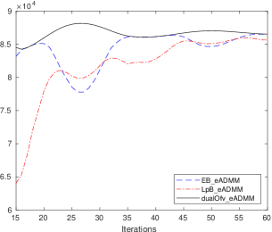
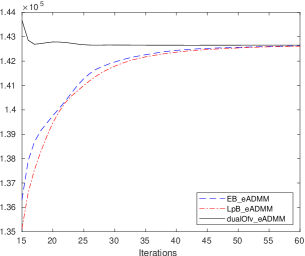

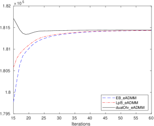
Figure 1 shows how the lower bounds from the post-processing methods evolve as the number of iterations of the extended ADMM increases. We used the DNN relaxation on an instance of the -equipartition problem of size and . There are three lines: EB_eADMM represents the lower bounds obtained by the rigorous lower bound method given in Algorithm 3, LpB_eADMM represents the linear programming bound given in Algorithm 2 and dualOfv_eADMM displays the approximate dual objective function value obtained by our extended ADMM. Figure 1a shows that the rigorous error bound method gives tighter bounds in general, while the linear programming bound method is more stable and less affected by the quality of the dual objective function value. The other figures indicate that for small , the rigorous error bound method gives tighter bounds (see Figure 1b), but as increases, the linear programming bound method dominates (see Figure 1c and 1d).
6.3 Results for -equipartition
6.3.1 Comparison of the Lower Bounds using SDP, DNN and Transitivity Constraints
In this section we want to highlight the improvement of the bounds obtained from the relaxations introduced in Section 2. Note that the timings for computing these bounds are discussed later in Section 6.3.2.
In practice, adding all the transitivity constraints is computationally too expensive, we run a DNN-based loop instead. The idea is as follows.
-
1.
Solve the DNN (3) to obtain the solution .
-
2.
Add transitivity constraints that are most violated by to the relaxation.
-
3.
Solve the resulting relaxation and repeat adding newly violated constraints until the maximum number of iterations is reached or no more violated constraints are found.
Tables LABEL:tab:keq_lb_80, LABEL:tab:keq_lb_50 and LABEL:tab:keq_lb_20 compare the lower bounds obtained from the relaxations for the -equipartition problem. The improvements are calculated as and , respectively; a ‘’ indicates that no transitivity constraints violated by the SDP solution of problem (3) have been found. In [21] it has been observed that the violation of the transitivity constraints is small and the nonnegativity constraints are more important than when the partition number increases. In our experiments we also observe that the improvement due to the nonnegativity constraints gets even better as increases.
| Imp % | Imp % | |||||
|---|---|---|---|---|---|---|
| – | – | |||||
| – | – | |||||
| – | – | |||||
| – | – | |||||
| – | – | |||||
| – | – | |||||
| – | – | |||||
| – | – | |||||
| – | – | |||||
| – | – | |||||
| – | – | |||||
| – | – | |||||
| – | – | |||||
| – | – | |||||
| – | – |
| Imp % | Imp % | |||||
|---|---|---|---|---|---|---|
| – | – | |||||
| – | – | |||||
| – | – | |||||
| – | – | |||||
| – | – | |||||
| – | – | |||||
| – | – | |||||
| – | – | |||||
| – | – | |||||
| – | – | |||||
| – | – | |||||
| – | – | |||||
| – | – | |||||
| – | – |
| – | – | |||||
| – | – | |||||
| – | – | |||||
| – | – | |||||
| – | – | |||||
| – | – | |||||
| – | – | |||||
| – | – | |||||
| – | – | |||||
| – | – | |||||
| – | – | |||||
| – | – |
6.3.2 Comparisons between extended ADMM and Interior Point Methods (IPMs) on -equipartition
In this section we want to demonstrate the advantage of our extended ADMM over interior point methods. For our comparisons we use Mosek [1], one of the currently best performing interior point solvers.
Note that computing an equipartition for these graphs using commercial solvers is out of reach. For instance, Gurobi obtains for a graph with vertices and after 120 seconds a gap of at least 80 %, whereas we obtain gap up to at most 7 %.
We list the results for solving the SDP (2) using an ADMM, and the results when solving the DNN relaxation (3) by our extended ADMM and by Mosek. We run the experiments on randomly generated graphs with 80% density, the results are given in Table LABEL:tab:time_keq.
| ADMM | Mosek | |||||
|---|---|---|---|---|---|---|
| SDP (2) | DNN (3) | DNN (3) | ||||
| Iter | CPU time | Iter | CPU time | CPU time | ||
| () | () | () | ||||
| – | ||||||
| – | ||||||
| – | ||||||
| – | ||||||
| – | ||||||
| – | ||||||
| – | ||||||
| – | ||||||
| – | ||||||
| – | ||||||
| – | ||||||
| – | ||||||
| – | ||||||
| – | ||||||
| – | ||||||
| – | ||||||
| – | ||||||
| – | ||||||
| – | ||||||
| – | ||||||
| – | ||||||
| – | ||||||
| – | ||||||
| – | ||||||
| – | ||||||
| – | ||||||
| – | ||||||
| – | ||||||
| – | ||||||
| – | ||||||
| – | ||||||
| – | ||||||
| – | ||||||
| – | ||||||
| – | ||||||
| – | ||||||
| – | ||||||
| – | ||||||
| – | ||||||
| – | ||||||
| – | ||||||
| – | ||||||
| – | ||||||
| – | ||||||
| – | ||||||
| – | ||||||
| – | ||||||
| – | ||||||
| – | ||||||
| – | ||||||
| – | ||||||
| – | ||||||
| – | ||||||
| – | ||||||
| – | ||||||
| – | ||||||
| – | ||||||
| – | ||||||
| – | ||||||
| – | ||||||
| – | ||||||
| – | ||||||
| – | ||||||
| – | ||||||
| – | ||||||
Table LABEL:tab:time_keq shows that the convergence behavior of the extended ADMM is not worse than the 2-block ADMM for SDP problems, and we can get a tighter lower bound by forcing nonnegativity constraints in the model without higher computational expense.
The results for Mosek solving problem (3) clearly show that these problems are out of reach for interior point solvers. A “” indicates that Mosek failed to solve this instance due to memory requirements.
6.3.3 Heuristics on -equipartition Problems
We now compare the heuristics introduced in Section 5 to get upper bounds for the graph partition problems.
We use the solutions obtained from the DNN relaxation to build upper bounds for the -equipartition problem since the experimental results in Section 6.4.1 showed that the DNN relaxation has a good tradeoff between quality of the bound and solution time.
We compare to the best know primal solution given in [2]; we set the time limit for our heuristics to 5 seconds. The gaps between the upper bounds by Vc+2opt (resp. Hyp+2opt) and the best know solution are shown in Table LABEL:tab:keq_armbruster. The primal bounds that are proved to be optimal are marked with “∗”.
| Graph | Vc+2opt | Gap | Hyp+2opt | Gap | Best Bound | ||
|---|---|---|---|---|---|---|---|
| 500 | 2 | ||||||
| 500 | 2 | ||||||
| 500 | 2 | ||||||
| 500 | 2 | ||||||
| 1000 | 2 | ||||||
| 1000 | 2 | ||||||
| 1000 | 2 | ||||||
| 1000 | 2 | ||||||
| 124 | 2 | ||||||
| 124 | 2 | ||||||
| 124 | 2 | ||||||
| 124 | 2 | ||||||
| 250 | 2 | ||||||
| 250 | 2 | ||||||
| 250 | 2 | ||||||
| 250 | 2 | ||||||
| 500 | 2 | ||||||
| 500 | 2 | ||||||
| 500 | 2 | ||||||
| 500 | 2 | ||||||
| 1000 | 2 | ||||||
| 1000 | 2 | ||||||
| 1000 | 2 | ||||||
| 1000 | 2 | ||||||
| mesh.138.232 | 138 | 2 | |||||
| mesh.148.265 | 148 | 2 | |||||
| mesh.274.469 | 274 | 2 | |||||
| mesh.70.120 | 70 | 2 | |||||
| mesh.74.129 | 74 | 2 |
Table LABEL:tab:keq_armbruster shows that on small instances our heuristics can find upper bounds not worse than the best known upper bounds. For large instances, Vc+2opt performs better than Hyp+2opt. The corresponding upper bounds are less than 10 % away from the best known upper bounds, some of them computed using 5 hours.
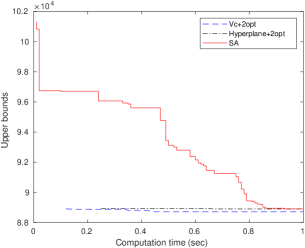
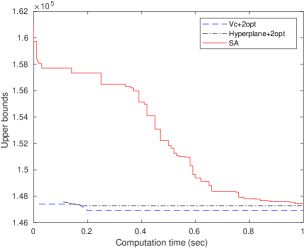
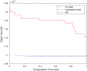
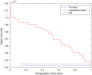
We next compare the upper bounds for the instances rand80, rand50, and rand20. Figure 2 shows that, for small instances (i.e., ), our hybrid methods (eg. Vc+2opt and Hyp+2opt) can find tight upper bounds quickly while simulated annealing (SA) needs a longer burning down time to achieve an upper bound of good quality.
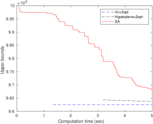
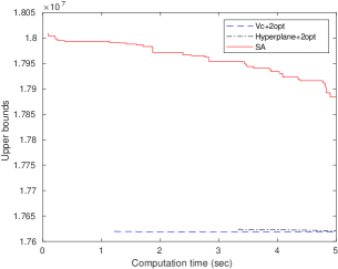
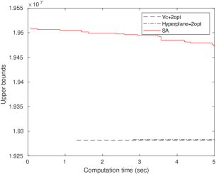
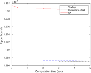
Figure 3 shows how the heuristics behave for large-scale instances (i.e, ). The time limit is set to 5 seconds. Compared to Figure 2, Vc+2opt and Hyp+2opt take more time to generate the first upper bounds but these upper bounds are much tighter than the one found by SA. Also, when the time limit is reached, the upper bounds found by Vc+2-opt and Hyp+2opt are much tighter than those from SA.
Tables LABEL:tab:keq_ub, LABEL:tab:keq_ub_50 and LABEL:tab:keq_ub_20 give a detailed comparison of the upper bounds for the instances rand80, rand50, and rand20, respectively. We display the gap between the lower bounds obtained from the DNN relaxation (3) and the upper bounds built by varied heuristics. The time limit for the heuristics is set to 1 second for and 3 seconds for for rand80. For rand50 and rand20 we set the limit to 5 seconds. The best upper bounds are typeset in bold.
The numbers confirm that Vc+2opt and Hyp+2opt can build tighter upper bounds than SA, in particular for the dense graphs rand80. Overall, Vc+2opt has the best performance.
Comparing lower and upper bounds, the numerical results show that our methods perform very well on dense graphs; for rand80 the largest gap is less than 4%, for rand50 the largest gap is less than 6%. As the randomly generated graph gets sparser, the gap between lower bounds and upper bounds increases, for rand20 the gap is bounded by 12%.
| Vc+2opt | Gap | Hyp+2opt | Gap | SA | Gap | |||
| 100 | 2 | |||||||
| 4 | ||||||||
| 5 | ||||||||
| 10 | ||||||||
| 20 | ||||||||
| 25 | ||||||||
| 200 | 2 | |||||||
| 4 | ||||||||
| 5 | ||||||||
| 10 | ||||||||
| 20 | ||||||||
| 40 | ||||||||
| 900 | 2 | |||||||
| 5 | ||||||||
| 10 | ||||||||
| 20 | ||||||||
| 30 | ||||||||
| 50 | ||||||||
| 100 | ||||||||
| 300 | ||||||||
| 1000 | 2 | |||||||
| 5 | ||||||||
| 10 | ||||||||
| 20 | ||||||||
| 40 | ||||||||
| 50 | ||||||||
| 100 | ||||||||
| 200 |
| Vc+2opt | Gap | Hyp+2opt | Gap | SA | Gap | |||
|---|---|---|---|---|---|---|---|---|
| 100 | 2 | |||||||
| 4 | ||||||||
| 5 | ||||||||
| 10 | ||||||||
| 20 | ||||||||
| 25 | ||||||||
| 200 | 2 | |||||||
| 4 | ||||||||
| 5 | ||||||||
| 10 | ||||||||
| 20 | ||||||||
| 40 | ||||||||
| 900 | 2 | |||||||
| 5 | ||||||||
| 10 | ||||||||
| 20 | ||||||||
| 30 | ||||||||
| 50 | ||||||||
| 1000 | 2 | |||||||
| 5 | ||||||||
| 10 | ||||||||
| 20 | ||||||||
| 40 | ||||||||
| 50 |
Comparing Tables LABEL:tab:keq_ub, LABEL:tab:keq_ub_50 and LABEL:tab:keq_ub_20, it can be observed that the gaps get larger as the graph gets sparser. We conjecture that this is due to less tightness of the lower bound which is supported by the following experiment.
We regard the best upper bounds obtained from all three heuristics within an increased time limit of 10 seconds. In this way, we should have an upper bound that approximates the optimal solution well enough for all densities. As an example, in Table LABEL:tab:keq_rand_100_5 we report for a graph on 100 vertices and three different densities the lower and these upper bounds. We can clearly see that when the graph gets sparser, adding the nonnegativity constraints to the SDP relaxation (2) gains more improvement. However, the gap between lower and upper bound gets worse as the graph gets sparser.
| Density | Improvement | Gap | |||
|---|---|---|---|---|---|
| 80 | 2.92 | ||||
| 50 | 4.83 | ||||
| 20 | 8.87 |
6.4 Results for GPKC
6.4.1 Comparison of the Lower Bounds using SDP, DNN and Transitivity Constraints
We now turn our attention to the GPKC problem. We run experiments similar to those presented in Section 6.3.1, i.e., we solve DNN (7) to obtain the solution . Table LABEL:tab:gpkc-lb shows the lower bounds for GPKC problems on the randomly generated graphs rand80. The improvements are calculated in the same way as in the previous section. The experimental results on GPKCrand50 and GPKCrand20 are omitted since they have a similar behavior.
The lower bounds obtained from different SDP relaxations show that when the capacity bound decreases (and thus the number of groups increases), the improvement of the nonnegativity constraints gets more significant. This is in line with the results for -equipartition. And, also similar to -equipartition, for GPKC the improvement due to the transitivity constraints is only minor.
| 26536 | ||||||
| 14023 | ||||||
| 11434 | ||||||
| 6321 | ||||||
| 3668 | ||||||
| 3043 | ||||||
| 50084 | ||||||
| 25787 | ||||||
| 21741 | ||||||
| 11404 | ||||||
| 6686 | ||||||
| 3419 |
6.4.2 Comparisons between extended ADMM and IPMs for GPKC
Table LABEL:tab:gpkc_time compares the computation times when solving the DNN relaxations for the GPKC (7) by the extended ADMM and Mosek, respectively. A “–” indicates for extended ADMM that the maximum number of iterations is reached, and for Mosek that the instance could not be solved due to memory requirements. The results of the SDP relaxation (6) in Table LABEL:tab:gpkc-lb are computed using Mosek, hence we omit these timings in Table LABEL:tab:gpkc_time.
In the thesis [19], numerical results on the GPKC are presented using an LP relaxation. However, the method therein is capable of getting bounds either for very sparse graphs of density at most 6 % (up to 2000 vertices) or for graphs with up to 140 vertices and density of at most 50 %. We clearly outperform these results in terms of the density of the graphs that can be considered.
| extended ADMM | Mosek | |||
|---|---|---|---|---|
| DNN (6) | DNN (6) | |||
| Iterations | CPU time | CPU time | ||
| () | () | |||
| – | – | |||
| 2167 | ||||
| 2241 | ||||
| 2369 | ||||
| 2760 | ||||
| 3198 | ||||
| 4918 | ||||
| 3257 | ||||
| 3431 | ||||
| 3760 | ||||
| 3564 | ||||
| 3538 | ||||
| – | – | – | ||
| 4837 | – | |||
| 5798 | – | |||
| 5820 | – | |||
| 5191 | – | |||
| 4010 | – | |||
| 4728 | – | |||
| 5355 | – | |||
| – | – | – | ||
| 4837 | – | |||
| 5798 | – | |||
| 5820 | – | |||
| 5191 | – | |||
| 4010 | – | |||
| 4728 | – | |||
| 5355 | – | |||
| – | – | – | ||
| 10061 | – | |||
| 8710 | – | |||
| 8982 | – | |||
| 9834 | – | |||
| 7054 | – | |||
| 6858 | – | |||
While for instances of size , the timings of the extended ADMM and Mosek are comparable, the picture rapidly changes as increases. For , Mosek cannot solve any instance while the extended ADMM manages to obtain bounds for instances with within one hour.
6.4.3 Heuristics on GPKC problems
As mentioned in Section 5, the simulated annealing heuristic for the QAP cannot be applied to the GPKC, because there is no equivalence between the GPKC and the QAP. Therefore, we compare the upper bounds for the GPKC from the heuristic introduced in Section 5.3 with the lower bounds given by the DNN relaxation (7). We set a time limit of 5 seconds.
Also, we set the maximum number of iterations to be 50 000 for the sparse graph GPKCrand20, while the maximum numbers of iterations for GPKCrand50 and GPKCrand80 are 20 000. In Table LABEL:tab:gpkc_ub, LABEL:tab:gpkc_ub_50 and LABEL:tab:gpkc_ub_20, a ∗ indicates for the extended ADMM that the maximum number of iterations is reached.
Table LABEL:tab:gpkc_ub shows that the gaps between the lower and upper bounds are less than 3% for GPKCrand80, they are less than 7% for GPKCrand50, see Table LABEL:tab:gpkc_ub_50, and for GPKCrand20, the gaps are less than 15%, see Table LABEL:tab:gpkc_ub_20. Similar to the -equipartition problem, we note that computing the lower bound on the sparse instances is harder. The maximum number of iterations is reached for rand20 much more often than for rand80 or rand50.
| VC+2opt | Gap | |||
|---|---|---|---|---|
| VC+2opt | Gap | |||
|---|---|---|---|---|
| VC+2opt | Gap | |||
|---|---|---|---|---|
7 Conclusions
In this paper we first introduce different SDP relaxations for -equipartition problems and GPKC problems. Our tightest SDP relaxations, problems (4) and (8), contain all nonnegativity constraints and transitivity constraints, which bring constraints in total. Another kind of tight SDP relaxation, (3) and (7), has only nonnegativity constraints. While it is straight forward to consider the constraint in a 3-block ADMM, including all the transitivity constraints is impractical. Therefore, our strategy is to solve (3) and (7) and then adding violated transitivity constraints in loops to tighten both SDP relaxations.
In order to deal with the SDP problems with inequality and bound constraints, we extend the classical 2-block ADMM, which only deals with equations, to the extended ADMM for general SDP problems. This algorithm is designed to solve large instances that interior point methods fail to solve. We also introduce heuristics that build upper bounds from the solutions of the SDP relaxations. The heuristics include two parts, first we round the SDP solutions to get a feasible solution for the original graph partition problem, then we apply 2-opt methods to locally improve this feasible solution. In the procedure of rounding SDP solutions, we introduce two algorithms, the vector clustering method and the generalized hyperplane rounding method. Both methods perform well with the 2-opt method.
The extended ADMM can solve general SDP problems efficiently. For SDP problems with bound constraints, the extended ADMM deals with them separately from inequalities and equations, thereby solving the problems more efficiently. Mosek fails to solve the DNN relaxations of problems with due to memory requirements while the extended ADMM can solve the DNN relaxations for -equipartition problems on large instances up to within as few as 5 minutes and for GPKC problems up to within as little as 1 hour.
We run numerical tests on instances from the literature and on randomly generated graphs with different densities. The results show that SDP relaxations can produce tighter bounds for dense graphs than sparse graphs. In general, the results show that nonnegativity constraints give more improvement when increases.
We compare our heuristics with a simulated annealing method in the generation of upper bounds for -equipartition problems. Our heuristics obtain upper bounds displaying better quality within a short time limit, especially for large instances. Our methods show better performance on dense graphs, where the final gaps are less than 4% for graphs with 80% density, while the gaps between lower and upper bounds for sparse graphs with 20% density are bounded by 12%. This is mainly due to the tighter lower bounds for dense graphs.
Acknowledgments
We thank Kim-Chuan Toh for bringing our attention to [13] and for providing an implementation of the method therein. We would like to thank the reviewers for their thoughtful comments and efforts towards improving this paper.
References
- ApS [2020] MOSEK ApS. The MOSEK optimization toolbox for MATLAB manual. Version 9.1.13, 2020. URL http://docs.mosek.com/9.1.13/toolbox/index.html.
- Armbruster [2007] Michael Armbruster. Branch-and-Cut for a Semidefinite Relaxation of Large-scale Minimum Bisection Problems. 2007.
- Chen et al. [2016] Caihua Chen, Bingsheng He, Yinyu Ye, and Xiaoming Yuan. The direct extension of ADMM for multi-block convex minimization problems is not necessarily convergent. Mathematical Programming, 155(1-2):57–79, 2016.
- De Santis et al. [2018] Marianna De Santis, Franz Rendl, and Angelika Wiegele. Using a factored dual in augmented Lagrangian methods for semidefinite programming. Operations Research Letters, 46(5):523–528, 2018.
- de Souza [1993] Cid Carvalho de Souza. The graph equipartition problem: Optimal solutions, extensions and applications. PhD thesis, PhD-Thesis, Université Catholique de Louvain, Louvain-la-Neuve, Belgium, 1993.
- Fan and Pardalos [2010] Neng Fan and Panos M Pardalos. Linear and quadratic programming approaches for the general graph partitioning problem. Journal of Global Optimization, 48(1):57–71, 2010.
- Frieze and Jerrum [1995] Alan Frieze and Mark Jerrum. Improved approximation algorithms for MAX -CUT and MAX bisection. In International Conference on Integer Programming and Combinatorial Optimization, pages 1–13. Springer, 1995.
- Garey et al. [1974] Michael R Garey, David S Johnson, and Larry Stockmeyer. Some simplified NP-complete problems. In Proceedings of the sixth annual ACM symposium on Theory of computing, pages 47–63, 1974.
- Ghaddar et al. [2011] Bissan Ghaddar, Miguel F Anjos, and Frauke Liers. A branch-and-cut algorithm based on semidefinite programming for the minimum -partition problem. Annals of Operations Research, 188(1):155–174, 2011.
- Goemans and Williamson [1995] Michel X Goemans and David P Williamson. Improved approximation algorithms for maximum cut and satisfiability problems using semidefinite programming. Journal of the ACM (JACM), 42(6):1115–1145, 1995.
- Helmberg et al. [1996] Christoph Helmberg, Franz Rendl, and Robert Weismantel. Quadratic knapsack relaxations using cutting planes and semidefinite programming. In International Conference on Integer Programming and Combinatorial Optimization, pages 175–189. Springer, 1996.
- Hendrickson and Kolda [2000] Bruce Hendrickson and Tamara G Kolda. Graph partitioning models for parallel computing. Parallel computing, 26(12):1519–1534, 2000.
- Jansson et al. [2007] Christian Jansson, Denis Chaykin, and Christian Keil. Rigorous error bounds for the optimal value in semidefinite programming. SIAM Journal on Numerical Analysis, 46(1):180–200, 2007.
- Johnson et al. [1989] David S Johnson, Cecilia R Aragon, Lyle A McGeoch, and Catherine Schevon. Optimization by simulated annealing: An experimental evaluation; part i, graph partitioning. Operations research, 37(6):865–892, 1989.
- Lin [1965] Shen Lin. Computer solutions of the traveling salesman problem. Bell System Technical Journal, 44(10):2245–2269, 1965.
- Lisser and Rendl [2003] Abdel Lisser and Franz Rendl. Graph partitioning using linear and semidefinite programming. Mathematical Programming, 95(1):91–101, 2003.
- Lorenz and Tran-Dinh [2018] Dirk A Lorenz and Quoc Tran-Dinh. Non-stationary Douglas-Rachford and alternating direction method of multipliers: adaptive stepsizes and convergence. arXiv preprint arXiv:1801.03765, 2018.
- Malick et al. [2009] Jérôme Malick, Janez Povh, Franz Rendl, and Angelika Wiegele. Regularization methods for semidefinite programming. SIAM Journal on Optimization, 20(1):336–356, 2009.
- Nguyen [2016] Dang Phuong Nguyen. Contributions to graph partitioning problems under resource constraints. PhD thesis, 2016.
- Nishihara et al. [2015] Robert Nishihara, Laurent Lessard, Ben Recht, Andrew Packard, and Michael Jordan. A general analysis of the convergence of ADMM. In International Conference on Machine Learning, pages 343–352, 2015.
- Rendl [1999] Franz Rendl. Semidefinite programming and combinatorial optimization. Applied Numerical Mathematics, 29(3):255–281, 1999.
- Sotirov [2012] Renata Sotirov. SDP relaxations for some combinatorial optimization problems. In Handbook on Semidefinite, Conic and Polynomial Optimization, pages 795–819. Springer, 2012.
- Sun et al. [2019] Defeng Sun, Kim-Chuan Toh, Yancheng Yuan, and Xin-Yuan Zhao. SDPNAL+: A matlab software for semidefinite programming with bound constraints (version 1.0). Optimization Methods and Software, pages 1–29, 2019.