Towards Performance Clarity of Edge Video Analytics

Abstract.

Edge video analytics is becoming the solution to many safety and management tasks. Its wide deployment, however, must first address the tension between inference accuracy and resource (compute/network) cost. This has led to the development of video analytics pipelines (VAPs), which reduce resource cost by combining DNN compression/speedup techniques with video processing heuristics. Our measurement study, however, shows that today’s methods for evaluating VAPs are incomplete, often producing premature conclusions or ambiguous results. This is because each VAP’s performance varies substantially across videos and time, and is sensitive to different subsets of video content characteristics.

We argue that accurate VAP evaluation must first characterize the complex interaction between VAPs and video characteristics, which we refer to as VAP performance clarity. We design and implement Yoda, the first VAP benchmark to achieve performance clarity. Using primitive-based profiling and a carefully curated benchmark video set, Yoda builds a performance clarity profile for each VAP to precisely define its accuracy/cost tradeoff and its relationship with video characteristics. We show that Yoda substantially improves VAP evaluations by (1) providing a comprehensive, transparent assessment of VAP performance and its dependencies on video characteristics; (2) explicitly identifying fine-grained VAP behaviors that were previously hidden by large performance variance; and (3) revealing strengths/weaknesses among different VAPs and new design opportunities.

1. Introduction

Edge video analytics is becoming the modern solution to many critical tasks (videoanalyticsapp, ). With the ability to accurately detect, recognize and track objects on the fly, it can quickly detect and respond to traffic accidents and hazard events (trafficvision, ; traffictechnologytoday, ; goodvision, ; intuvisiontech, ; vision-zero, ; visionzero-bellevue, ; msr-bellevue, ), monitor and enforce physical distance during COVID-19 (cameracovid, ; cameracovid1, ), auto-manage retail stores and factories (smartretail, ), and perform surveillance functions to make the world safer (ChicagoCam, ; LondonCCTV, ).

Deployment of edge video analytics at scale, however, must address the tension between inference accuracy and resource cost, i.e., compute cost to run inference tasks and/or bandwidth cost to transfer data from cameras to servers (chen2019deep, ; noghabi2020emerging, ). This tension continues to grow as video sources proliferate at the network’s edge (ChicagoCam, ; LondonCCTV, ; VideoAnalyticsMarket, ; slate-video-news, ; infowatch16, ), separated from the heavy compute power necessary to run large deep neural networks (DNNs) by a bandwidth-constrained mobile network.

In response, researchers have developed numerous video analytics pipelines (VAPs) to optimize the accuracy and cost tradeoff (noscope, ; chameleon, ; fast, ; videostorm, ; mainstream, ; videoedge, ; mcdnn, ; glimpse, ; awstream, ; dds-hotcloud, ; rexcam-hotmobile, ; vigil, ; emmons2019cracking, ; eaar, ), by combining DNN model compression/speedup techniques with video processing heuristics such as frame sampling and image downsizing (see Figure 1). For instance, Chameleon (chameleon, ) shows that intelligently subsampling traffic video frames at the cameras can effectively reduce network and compute costs without degrading inference accuracy.

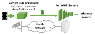
Figure 1. Illustration of a video analytics pipeline (VAP).

As edge video analytics and VAPs continue to evolve, accurate and transparent evaluation of VAPs becomes critical. For instance, operators of edge video analytics need to know what the optimal VAP is for a given video input, how often the network/compute usage exceeds a budget, or how often accuracy drops below a threshold.

Evaluating VAPs:  Today, VAPs are evaluated using some corpus of past video samples that represent the target scenario(s). After running VAPs on these videos, their performance (i.e., the accuracy and cost tradeoff) is analyzed and compared against each other. Following this method, we run an empirical study to evaluate seven VAPs from recent papers, using a large chunk (14.5 hours) of traffic videos. Our study shows that today’s evaluation method is insufficient to characterize VAPs, often leading to partial/premature conclusions on the efficacy of a VAP and across VAPs. This is because VAP performance has a strong dependency on video content – it can vary substantially across videos even in the same scenario (e.g., highway traffic cameras), and drift dramatically over time when operating on the same camera. Therefore, today’s evaluation is either biased by the use of short video clips or produces vague results over long videos, i.e., an excessively wide distribution of possible cost-accuracy outcomes.

Our measurement study suggests that an ideal evaluation of VAPs must have high performance coverage and low performance variance. Here, “high coverage” means the evaluation reveals both good and bad performance of a VAP, whereas “low variance” means the evaluation could accurately estimate the VAP’s performance on individual videos. And the strong dependency of VAP performance on video content suggests such ideal evaluation must characterize the complex interactions between video workloads and a VAP’s performance. Doing so presents three distinct benefits for VAP design and deployment: (1) providing a comprehensive assessment of VAPs under diverse video characteristics; (2) understanding how/why each VAP’s performance varies across videos; (3) revealing relative strengths among VAPs under different video content characteristics. We refer to this new evaluation requirement as VAP performance clarity.

Achieving performance clarity:  A direct approach would test VAPs exhaustively on a large collection of mobile video workloads, e.g. existing video collections developed for testing DNN models (imagenet, ; coco, ; google-benchmark, ; tbd, ; dawnbench, ; visual-road, ; coleman2019analysis, ). Yet these are designed to evaluate DNN architectures rather than VAPs, thus lack sufficient coverage of video characteristics that will affect VAP performance. An alternative is to build a database of empirical workloads that covers all possible video feature value combinations, and use them to test VAPs. This is intractable, however, since it would require a large database capturing an exponential number of video feature combinations.

Instead, we propose to characterize VAP performance using a carefully curated set of videos that serve to evaluate different aspects of VAPs. Our design is based on the observation that each VAP is inherently modular and can be broken into a set of “global” primitives. Each primitive leverages a distinct set of video processing heuristics to optimize the accuracy/cost tradeoff, and thus can be profiled independently (against its associated video features) and then (re)assembled to profile full VAPs. This modular structure allows us to efficiently profile each full VAP by combining its corresponding primitive-specific profiles. Note that some prior works also observe independent VAP modules but use it to refine particular VAP designs (videoedge, ; chameleon, ). In contrast, we leverage this observation to design accurate evaluation of many VAPs.

We present Yoda, the first VAP benchmark designed to achieve performance clarity. Using a carefully curated set of benchmark videos (67 minutes in length), Yoda focuses on characterizing the complex dependencies of VAP performance on mobile video content characteristics, and does so efficiently. For each VAP $v$, Yoda builds a performance clarity profile $(\mathbb{P}_{v})$ by running $v$ on a set of benchmark videos parameterized by a set of video features, both chosen based on $v$’s design primitives. The resulting $\mathbb{P}_{v}$ is a lookup table that lists $v$’s performance (the accuracy/cost relationship) under different video feature values. This provides a comprehensive and transparent assessment of $v$’s performance and its dependencies on video features. We show Yoda’s contributions towards VAP evaluation, in three concrete aspects.

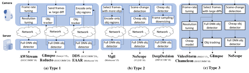
Figure 2. Schematic illustration of some example VAPs grouped into three general types. (Differences within each general scheme are omitted here.) Our goal is not to list all VAPs; instead, we seek to identify common techniques and their performance.

• Performance clarity – Yoda accurately captures existing VAPs’ performance and their dependencies on video features. It largely outperforms existing VAP evaluations with higher coverage (the completeness of the evaluation) and lower variance (the ambiguity of the evaluation outcome).

• Performance prediction – Using $\mathbb{P}_{v}$, Yoda can efficiently estimate $v$’s performance for videos not included in the benchmark set, without running $v$. This takes 2 orders of magnitude less computation than running $v$ on the video.

• Practical insight for VAP deployment – Yoda’s VAP profiles expose strengths and weaknesses among existing VAPs, and the underlying deployment scenarios and video features associated with these conclusions. These insights allow us to identify previously hidden gaps and opportunities to guide/motivate future VAP designs.

Though Yoda serves well on the seven VAPs considered in this work, it is not without limitations. Currently, Yoda’s content features and benchmark videos are not future-proof (e.g., Yoda does not support multi-stream/multi-query VAPs). For distributed VAPs that handle bandwidth-constrained connections, Yoda only evaluates reductions in average network bandwidth usage but not the impact of bandwidth fluctuation.

Nonetheless, as the first attempt at benchmarking VAPs’ performance clarity, Yoda suggests a viable path towards profiling the dependencies of VAPs’ performance on video content via a modularized approach. Our goal is not to realize an “ideal” benchmark; rather, we provide a concrete implementation of the proposed benchmark, which validates the need for performance clarity and initial feasibility on accurate performance evaluations of VAPs, and provides new insights for VAP design and deployment. We release the Yoda toolkit in https://yoda.cs.uchicago.edu and plan to expand our study to include other VAPs and additional video features.

2. Background

In this section, we present an overview on existing VAPs, focusing on their design objectives and evaluations.

2.1. VAP Design

Computer-vision DNNs are generally optimized for high accuracy. However, the compute and network cost to achieve such accuracy can be high. This tension between accuracy and cost has stimulated many ongoing efforts to develop video analytics pipelines (VAPs) (awstream, ; chameleon, ; vigil, ; eaar, ; videostorm, ; mainstream, ; noscope, ; reducto, ; dds-sigcomm, ). VAPs reduce network/compute cost while maintaining high inference accuracy, by combining DNN compression/speedup methods and video processing heuristics such as frame sampling and image downsizing.

Existing VAPs fall in three general types (Figure 2).

• Type 1: Saving network cost when the camera has low local compute power. The camera only encodes video frames and runs simple tracking algorithms, but does not perform any inference that requires accelerators such as GPUs. Instead, a VAP saves network cost by selecting a subset of frames/pixels to send to the server for DNN inference. For example, AWStream (awstream, ) adapts video frame rate, resolution and quality. Glimpse (glimpse, ) and Reducto (reducto, ) send only frames that contain new objects (e.g., identified by measuring inter-frame difference). Similarly, EAAR (eaar, ) and DDS (dds-sigcomm, ) only encode regions that are likely relevant to the inference task.

• Type 2: Saving network cost when the camera and the server split the inference task. Here the camera device is equipped with some inference power (e.g., with a low-power GPU) and thus can run a cheap DNN. For example, Vigil (vigil, ) runs a cheap object detector on the camera to identify regions containing most objects and sends only these regions to the server for full DNN inference. NoScope (noscope, ) first identifies frames with significant pixel changes and runs a cheap DNN (fine-tuned per video stream) on these frames. Only when the cheap DNN has low confidence will the frames be sent to the server for further inference.

• Type 3: Saving compute cost of a resource-constrained edge device. The third type of VAPs reduces compute cost, when a camera device (or edge server) has moderate compute power to run some inference locally. Videostorm (videostorm, ) and Chameleon (chameleon, ) uniformly sample frames, downsize the sampled frames to a lower resolution, and process them using a less accurate yet cheaper DNN model. We note that Glimpse (Type 1), NoScope (Type 2) can also be applied here to reduce compute cost, and thus fall into this type.

2.2. How Are VAPs Evaluated Today?

Today’s evaluation empirically tests and compares the VAPs’ performance (accuracy, cost) on a set of videos collected from the target scenario(s) (noscope, ; videostorm, ; videoedge, ; chameleon, ), e.g., some traffic videos recorded by fixed cameras in urban crossroads. Table 1 lists the target scenarios and videos (sources and lengths) used to evaluate some recent VAPs.

Such evaluation relies on an implicit assumption:

• Today’s evaluation assumption: A VAP’s performance under a target scenario can be represented by its performance seen on a set of long videos of the same scenario.
  

Unfortunately, this is not always true. Our own measurement study shows that a VAP’s performance can vary dramatically among videos of the same scenario (see §3.2).

VAP	Target scenarios (sources of videos) “YT” = YouTube, “P” = proprietary	Total duration (# of videos)
Glimpse (glimpse, )	Moving traffic cams (YT) + Face (P)	65min (30)
AWStream (awstream, )	Fixed traffic cams (MOT16) + AR (P)	6.3min (4)
Vigil (vigil, )	Campus cams + Indoor (P)	3min (3)
Reducto (reducto, )	Fixed traffic cams (YT)	250min (25)
Chameleon (chameleon, )	Fixed traffic cams + Indoor (P)	525min (15)
DDS (dds-sigcomm, )	Fixed & Moving traffic cams (YT)	30.7min (16)

Table 1. Today, VAPs are evaluated on videos of one or two scenarios as a whole. For consistency, we only list object detection datasets.

3. Our Empirical Study on VAP Evaluation

As video analytics and VAPs continue to evolve, accurate and transparent evaluation of VAPs is crucial to their real-world adoption. In this work, we are interested in understanding whether today’s VAP evaluation methods (§2.2) can fulfill this requirement. Since existing VAP proposals generally run evaluation using different datasets, one cannot directly assess and compare their performance from their reported results. Instead, our empirical study evaluates 7 popular VAP designs using the same video datasets (14.5 hours in total) that consist of a much larger and more diverse collection of traffic videos. Our analysis reveals significant VAP performance variability across videos of the same target scenario, suggesting that today’s evaluation method is insufficient to characterize VAPs. We then discuss its implications for a better VAP evaluation, which lead to the development of Yoda.

3.1. Methodology and Dataset

We start by discussing the methodology behind our measurement study.

VAPs studied:  We study and compare the performance of 7 recent VAPs on the task of object detection. These include AWStream (awstream, ), Glimpse (glimpse, ), Vigil (vigil, ), NoScope (noscope, ), Videostorm (videostorm, ), Reducto (reducto, ), and DDS (dds-sigcomm, ). They cover a wide range of today’s VAP design techniques illustrated in Figure 2.

For consistency, we configure all these VAPs to operate on videos of (30fps, 720p) and all use the same pre-trained DNN model as their full DNN model. To choose the full DNN model, we experimente with several popular choices (e.g., FasterRCNN-ResNet101 (google-model-zoo, ), Yolo (yolov3, )) and select FasterRCNN-ResNet101 since it produces the highest accuracy in object detection. Later we also repeat our experiments using Yolo, and find that while the absolute VAP performance varies slightly, the key findings remain the same. Finally, we consider the scenario where VAPs are “optimally configured” to eliminate potential inconsistency or errors introduced by imperfect system configuration. For each video segment ($\approx$30s), we configure each VAP by picking its best parameter values (e.g., frame sampling rate of VideoStorm, or inter-frame difference threshold of Glimpse) that minimize cost while achieving over 0.9 inference accuracy in the first 1/3 of the segment. We then test and report the VAP performance on the rest of the video segment. We believe this consideration helps increase the fairness and transparency of our VAP evaluation.

Our “coverage” dataset:  To show a more complete picture of VAP performance, we compile a coverage set of public traffic videos from a diverse video sources at a much larger scale than existing works. We target specifically traffic videos since they are commonly used in VAP evaluation (see Table 1). When compiling our dataset, we seek to include public traffic videos from diverse sources, covering different scenarios (fixed or moving cameras; day or night; highway, city or rural streets), and videos displaying a wide range of content characteristics and dynamics, e.g., object speeds, sizes, object arrival rate.

With these in mind, our final coverage set consists of 14.5 hours of traffic videos from multiple sources: YouTube (32 long videos, 10-47 minutes each), Waymo (sun2019scalability, ) (5 hours), KITTI (Geiger2012CVPR, ) (20 minutes), and MOT (MOT16, ) (8 minutes). All videos are split into 2112 segments ($\approx$30s per segment).

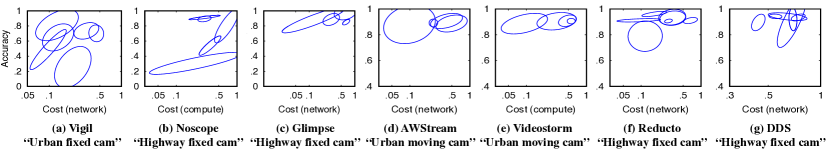
Figure 3. Significant performance variability of the same VAP among videos of the same scenario. Each ellipse outlines the 1-$\sigma$ range of VAP performance across the segments of a video.

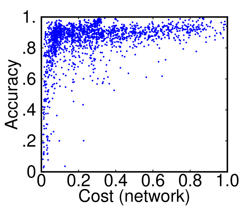
(a) AWStream (Type 1)

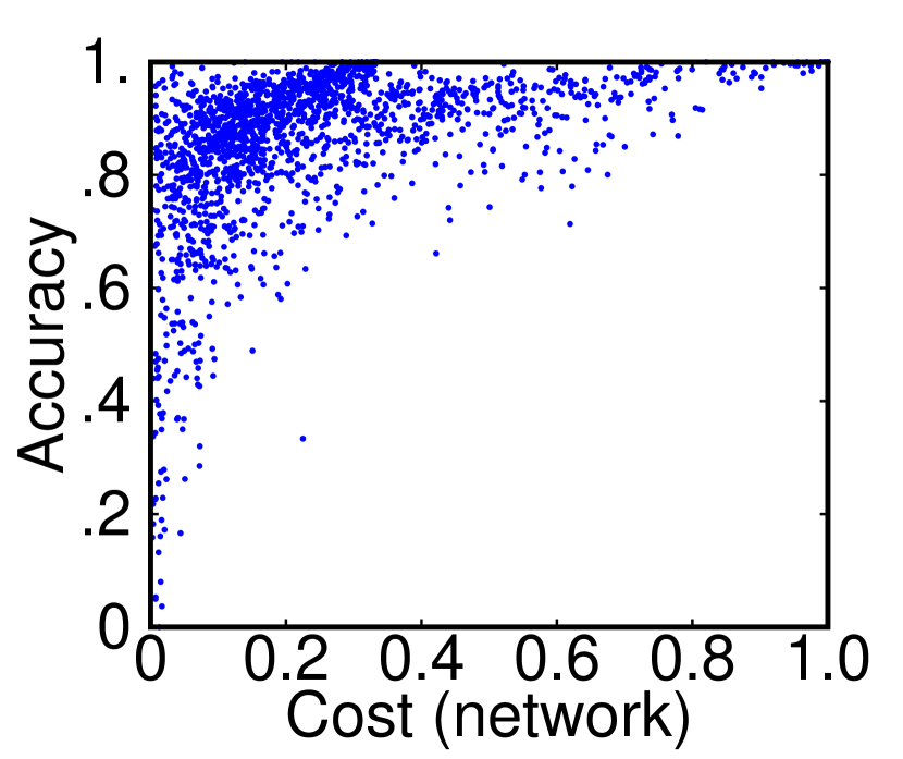
(b) Glimpse (Type 1)

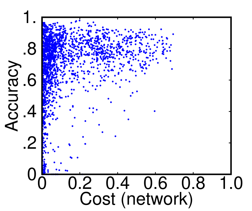
(c) Vigil (Type 2)

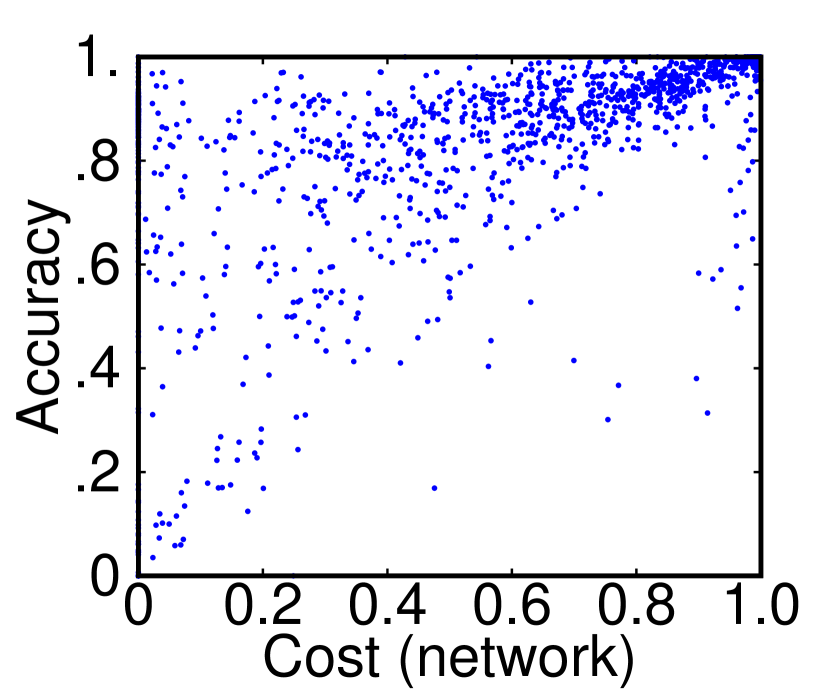
(d) NoScope (Type 2)

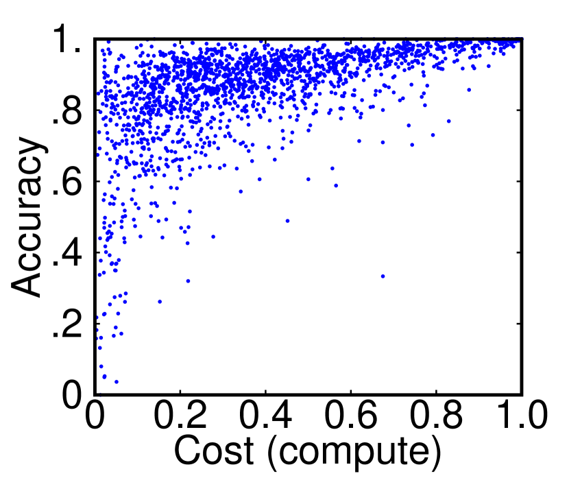
(e) Glimpse (Type 3)

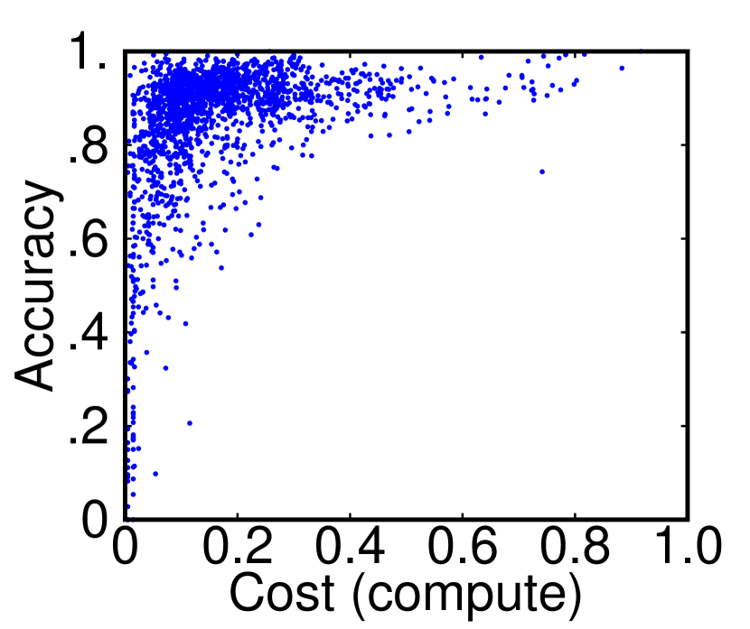
(f) VideoStorm (Type 3)

Figure 4. Significant performance variability across video segments. Each dot shows the accuracy and cost of a segment.

Performance metrics used:  We measure each VAP’s performance using the following three metrics:

• Accuracy is measured by the F1 score of a VAP’s detected objects (everingham2010pascal, ). We obtain the “ground truth” results by running the full DNN on the uncompressed video frames (rather than the human-annotated labels). This way, any inaccuracy will be due to VAP designs (e.g., video compression, DNN distillation), rather than errors made by the full DNN itself. This is consistent with recent work (e.g., (awstream, ; vigil, ; videostorm, ; chameleon, ; mullapudi2019online, ; noscope, )).

• Normalized network cost defines the data size sent by the camera to the server divided by the size of the original video. Reducing network cost is crucial when deploying VAPs in bandwidth-constrained networks (noghabi2020emerging, ).

• Normalized compute cost is the average GPU usage (on a NVidia GTX Titan Xp) per frame divided by that of the full DNN model. Since the cost is normalized against running the full DNN model on the same GPU, it is less dependent on the particular choice of GPU. Note that when a VAP (e.g., Glimpse) reduces both compute and network costs, we will specify which is being considered.

We acknowledge that there are other aspects of VAP performance beyond these metrics. Our choice of these metrics is based on two reasons. First, these metrics are directly related to video content. For example, evaluating things like how adaptive a VAP is to bandwidth variations is important but deviates from our main goal of understanding the impact of video content. Similarly, metrics like throughput, processing delay or energy consumption are crucial but also highly sensitive to the implementation details (e.g., pipelining or parallelization) and hardware platform. Second, these metrics can be translated into practical objectives. The feasibility of deploying a VAP depends on whether its costs fit the provisioned compute/network resources or the deployment budget. Although we do not evaluate other performance metrics (e.g., throughput, latency) explicitly, we believe they are highly correlated with the network and compute cost considered by our study. For example, when a VAP reduces network cost by 2x, this saving can translate into serving 2x video streams while meeting the same inference accuracy target (i.e., 2x throughput).

3.2. Key Findings

• Performance of a VAP can vary dramatically even among videos of the same scenario.
  

Following the traditional assumption (§2), we test each VAP’s performance (cost vs. accuracy) in one of the four scenarios: {fix-positioned traffic monitoring cameras, moving dashboard cameras} $\times$ {on urban streets, or on highway}. Figure 3 summarizes each VAP performance range in each video (each over 20 minutes) in one ellipse. We see each VAP’s performance can vary dramatically across videos in the same scenario. Such performance heterogeneity is prevalent across all 7 VAPs and four scenarios considered by our study.

To reveal the full range of performance variability, Figure 4 plots the performance distributions of the 5 VAPs on all the video segments in the coverage dataset (each dot shows the performance on one segment). While the overall trends align with findings of prior work (VAPs trade accuracy drop for saving network/compute cost), we do see that each VAP has a significant performance variability across video segments.

Cost when acc. is in [0.9, 0.95]	VAP type 1		VAP type 2		VAP type 3
	AWStream	Glimpse	Vigil	NoScope	Glimpse	VideoStorm
Mean	0.34	0.27	0.15	0.67	0.41	0.20
Relative StdDev	73%	64%	102%	48%	45%	68%

Table 2. Even when we narrow the range of accuracy in Figure 4 to [0.90,0.95], the cost (network or compute) across segments could vary significantly. This can be seen from the relative standard deviation values in the table.

Even when we restrict the accuracy to a small range ([0.90, 0.95]), the relative standard deviation of cost across segments can be 45-102% and the gap between $5^{\textrm{th}}$ and $95^{\textrm{th}}$ percentiles is always over 90% (shown in Table 2). Here, relative standard deviation is defined as the ratio of the standard deviation to the mean, which is a popular metric to measure the dispersion of a distribution.

• Choice of optimal VAP is content-dependent.
  

Performance variance does not always lead to suboptimal choice of VAP, if one VAP always outperforms others. Unfortunately, that is not true for VAPs. We illustrate this by comparing VAPs in pairs. In each pair, one VAP acts as a “reference”, and we subtract the other VAP’s cost and accuracy on each video segment by those of the reference. Figure 5 shows the results of three VAP pairs and marks the region where one VAP is strictly better than the other (higher accuracy and lower cost). Clearly, the choice of best VAP varies across video segments and is content-dependent. Thus, it is crucial for VAP operators and developers to understand under what videos would one VAP perform better than others.

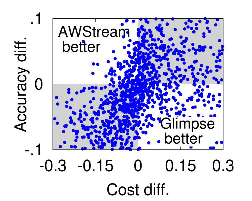
(a) AWStream vs.
Glimpse (Type 1)

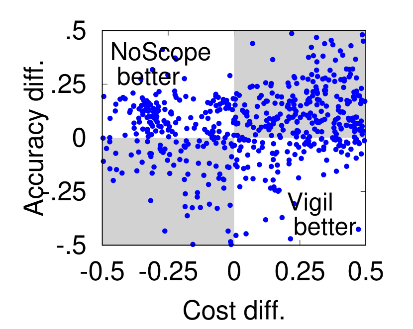
(b) NoScope vs.
Vigil (Type 2)

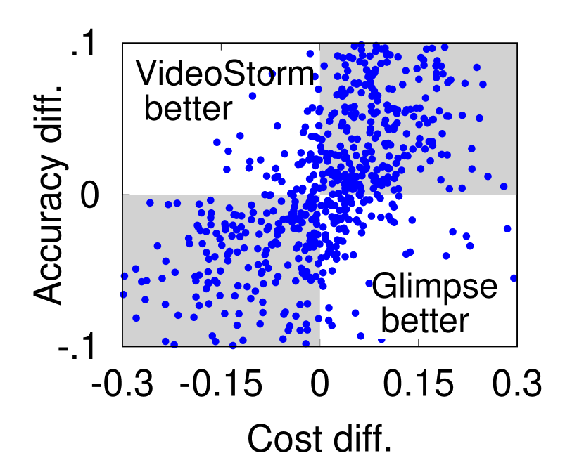
(c) VideoStorm vs.
Glimpse (Type 3)

Figure 5. Each VAP outperforms the other on many video segments. each dot shows the relative accuracy & cost between two VAPs on one video segment.

Together, these findings cast doubt over the current VAP evaluation methodology:

• Key Takeaway: Empirically testing and comparing VAPs on some specific video workloads can be incomplete.
  

3.3. Discussion

Our measurement has shown that if a VAP is evaluated on only a handful of videos, the results may fail to reveal its true performance range and variance in a target scenario. An immediate response is “why not using a better test dataset?”

Why not using a representative dataset?  Intuitively, with a set of “representative” videos per scenario, we can get the most common VAP performance by testing VAPs on these videos. Unfortunately, this solution is impractical for two reasons. First, cameras deployed at different locations or future locations will likely generate video workloads with different content characteristics beyond those captured by the empirical tests. Second, since video analytics applications are continuously evolving, representative workloads do not yet exist. Thus, these tests might overestimate/underestimate the VAP performance and lead to wrong choice of VAP in deployment.

Why not using a larger dataset?  Testing a VAP on a larger number of videos might offer a more complete view of its performance range and variance. Yet a “just adding data” approach will provide little insight on performance distribution on videos outside of the test dataset, and why a VAP’s performance varies across videos.

4. Achieving Performance Clarity

Different from prior work that evaluates VAPs using only empirical tests, we propose a new methodology for VAP evaluation: achieving performance clarity. The goal of performance clarity is to not only identify a VAP’s performance under a wide range of video content, but also characterize how video content characteristics affect its performance. This produces a comprehensive and transparent assessment of VAP performance. In the following, we first present the key concept behind performance clarity and its benefits, and then discuss potential solutions to achieve performance clarity.

To facilitate the discussion below, Table 3 summarizes the key terminologies and notations used by our work.

Terminology	Definition
Video content features	Features that measure content-level characteristics of a video (e.g., avg object speed). See §5.2.
Performance Clarity (PC)	Comprehensive performance assessment of VAPs under different video content features. See §4.1.
PC Profile ($\mathbb{P}_{v}$)	A lookup table that maps video content features to performance of VAP $v$ (e.g., Figure 6)
Cost-saving Strategy	A particular heuristic to save computer/network cost. See §5.1.
VAP Primitives	A set of cost-saving strategies that seek to reduce same type of redundancies. See §5.1.

Table 3. Definition of terminologies used in Yoda.

4.1. Defining Performance Clarity (PC)

The performance clarity (PC) of a VAP defines how video content features affect the VAP’s performance. Formally, PC of a VAP $v$ is a lookup table $\mathbb{P}_{v}$ that maps from a point $x$ in the space of video content features to $v$’s performance (in cost and accuracy) on videos that match $x$. This is illustrated by Figure 6. Compared to existing evaluations that are either incomplete (e.g., single-scenario tests in Figure 3) and/or ambiguous (e.g., high performance variability in Figure 4), PC offers a comprehensive and clear characterization of VAP performance and its variation.

The key insight behind PC is the following. It is the VAP performance’s dependencies on video content features that cause the VAP performance variabilities. As these content features vary across videos (in the same scenario), so does VAP performance. To illustrate this, we featurize each video in our coverage dataset along four content features (more features discussed later in §5.2), and plot in Figure 7 the Pearson’s correlation coefficients between individual features and cost of VAPs when keeping accuracy between 0.9 and 0.95 (to avoid cost variance caused by accuracy variance). We single out the impact of each feature by restricting other features to a small range less than 50% of their respective value ranges. The results show a strong correlation between each VAP’s performance and the content features.

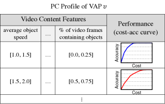
Figure 6. An abstract illustration of a VAP $v$’s performance clarity (PC) profile. Compared to either testing a VAP on few videos or reporting its performance distribution over many videos, this profile provides a more complete picture of the VAP’s performance by describing its relationship with video content features, which drastically reduces the ambiguity of performance compared to those in Figure 4.

Benefits of PC:  A VAP $v$’s performance variation and its content dependency come from the $v$’s design, i.e. they are inherent to $v$. Thus $v$’s PC profile ($\mathbb{P}_{v}$) can offer useful insights on its design and deployment. Below are two usage cases.

• To estimate $v$’s performance on any target video, we can directly combine $\mathbb{P}_{v}$ with the content feature distribution of the video, which can be quickly obtained by scanning through the video. The computation cost is significantly less than running $v$ on the video (verified in §6).

• To identify when one VAP outperforms another, we can directly compare two VAPs’ PC profiles to identify in which parts of the content feature space is one VAP better. Again there is no need to run VAPs on any video.

Later in §6 we use these two tasks to evaluate the accuracy and benefits of our PC profiler Yoda.

4.2. Feature-based Profiling: Why It Fails

Building an accurate PC profile is challenging. A straightforward solution is to create a corpus of videos that span all combinations of relevant content feature values, and test VAPs on these videos. Unfortunately, this can be prohibitively expensive due to the complex relationship between VAP performance and content features. Specifically, our measurement study (e.g. Figure 7) lead to two observations.

• Heterogeneity impact of features: Different VAPs are affected by different sets of features. For example, VideoStorm is sensitive to average object speed ($f_{1}$) but not per-object area ($f_{3}$); yet NoScope is highly sensitive to $f_{3}$ but not $f_{1}$.

• Combinatorial impact of features: A VAP can be affected by multiple features. For instance, Glimpse is highly correlated with the features of object speed ($f_{1}$) and fraction of frames with objects ($f_{2}$), and AWStream is sensitive to $f_{1}$ and $f_{3}$. Therefore, it is insufficient to test VAPs on videos that vary along only one feature at a time.

Thus, to cover all possible feature value combinations, we need $O(n^{|\mathbb{F}|})$ videos, where $\mathbb{F}$ is the list of content features and $n$ is the number of possible values per feature. To put it into perspective, let us assume that there are 7 content features, each having 4 distinct value buckets (e.g., low, median, high and very high), and we need three 30-second videos to measure VAP performance for each of the $4^{7}$ feature value combinations. These are not overestimation: there are at least 7 content features that might affect DNN accuracy or VAP performance (see §5.2), and in our dataset we split each feature in four buckets as well. The resulting dataset would be over 400 hours, much longer than any VAP test datasets ever created. Since many VAPs do not reduce compute cost, evaluating their performance on this hypothetical dataset would take 400 hours even when using one NVidia GTX Titan X GPU card running the state-of-the-art object detector at 30fps (google-benchmark, ).

(a) VideoStorm

(b) AWStream

(c) Glimpse

(d) NoScope

Figure 7. Strong correlation between video content features and VAP performance. The four features are: ($f_{1}$) avg. object speed, ($f_{2}$) % of frames with objects, ($f_{3}$) 10%ile of per-object area, and ($f_{4}$) avg. confidence score per object.

4.3. Proposed: Primitive-based Profiling

Instead of profiling a VAP as a monolithic entity, we modularize it into multiple primitives (§5.1), each of which can be profiled separately. The rationale is two-fold.

• A primitive is affected by fewer features than a VAP. Each primitive only leverages, and is thus affected by, a particular set of video content characteristics. For example, many VAPs reduce video frame rates to save cost, and its efficacy depends only on temporal-related features like object speeds. Yet these features have little impact on “orthogonal” techniques like image downsizing or model compression.

• Primitives have independent impacts on a VAP’s performance. As we will show in §5.1, the performance of a VAP can be approximated by multiplying the performance of each primitive when other primitives are set to their corresponding most accurate, expensive strategies. In other words, these primitives can be profiled individually, based on which the full VAP performance can be constructed.

Reducing profiling cost:  Since each primitive is profiled using only the video features relevant to its cost-saving strategy, the VAP profiling overhead can be drastically reduced, from $O(n^{|\mathbb{F}|})$ to $O(n^{|\mathbb{F}_{1}|}+n^{|\mathbb{F}_{2}|}+\cdots)=O(n^{\textrm{max}_{i}|\mathbb{F}_{i}|})\ll O(n^{|\mathbb{F}|})$, where $\mathbb{F}_{i}$ is the feature set related to the $i^{\textrm{th}}$ primitive. Using primitive-based profiling, our eventual dataset consists of only 67.5 minutes of videos, more than two orders of magnitudes less than that of feature-based profiling (400 hours)!

5. Yoda: Practical VAP Profiling

We now describe our design of Yoda, the first VAP benchmark to achieve performance clarity. Yoda builds a PC profile for each VAP, by applying the aforementioned primitive-based profiling. In the following, we first present how Yoda modularizes a VAP into independent primitives (§5.1) and chooses content features and benchmark videos to profile each primitive (§5.2), followed by two core functions offered by Yoda: VAP profiler and VAP performance predictor (§5.3).

5.1. Modularizing VAPs into Primitives

A VAP may employ one or more cost-saving strategies to reduce redundancies in video frames, pixels, and DNN parameters. Observing this inherent modularity, Yoda categorizes these strategies into three primitives (see Table 4).

VAP	Temporal pruning	Spatial pruning	Model pruning
VideoStorm(videostorm, )	✔ (uniform sampling)	✔(quality downsize)	✔ (model selection)
NoScope(noscope, )	✔ (diff-triggered)		✔(specialization)
AWStream(awstream, )	✔ (uniform sampling)	✔(quality downsize)
Glimpse(glimpse, )	✔ (diff-triggered)		✔(fixed tiny model)
Vigil(vigil, )	✔ (diff-triggered)	✔ (region cropping)
Chameleon(chameleon, )	✔ (uniform sampling)	✔(quality downsize)	✔(model selection)
VideoEdge(videoedge, )	✔(uniform sampling)	✔(quality downsize)
DDS(dds-hotcloud, )		✔ (region cropping)
EAAR(eaar, )	✔ (diff-triggered)	✔ (region cropping)
Reducto(reducto, )	✔ (diff-triggered)
WEG(fast, )			✔(specialization)

Table 4. Modularizing some example VAPs into primitives.

• Primitive #1: Temporal pruning drops frames to reduce inter-frame redundancies using at least two strategies. Uniform frame selection (e.g., (awstream, ; videostorm, )) uniformly samples a fraction of frames for further analysis and then carries over their detected objects to future unsampled frames (e.g., via object tracking). It works well if neighboring frames are similar. Trigger-based frame selection (e.g., (noscope, ; glimpse, )) skips frames until a heuristic (e.g., significant difference between frames) signals potential arrivals of new objects. It works well when most frames have few objects of interest.

• Primitive #2: Spatial pruning reencodes video to reduce redundancies among pixels. Specifically, image quality downsizing (e.g., (awstream, ; chameleon, )) reduces the video quality (e.g., from 1080p to 360p), which still achieves high accuracy if objects are large. Another strategy, region cropping (e.g., (vigil, ; dds-hotcloud, )), saves bandwidth by encoding only pixels relevant to the task. It can be very effective in, for instance, traffic videos where most vehicles/pedestrians appear small.

• Primitive #3: Model pruning leverages the fact that videos often have specific object classes/scenes (e.g., traffic videos contain mostly vehicles/pedestrians with static background), and trims the full DNN to reduce compute cost while still achieving high accuracy. Model selection (e.g., (videostorm, ; chameleon, )) picks a simple yet accurate DNN model from a few pre-trained models with various capacities. Model specialization (e.g., (noscope, ; fast, )) trains a smaller DNN just for particular scenes/objects and if it fails, falls back to the full DNN.

Finally, for each primitive, Yoda also defines an oracle strategy that does no cost reduction: 100% frame selection (for temporal pruning, original video quality (for spatial pruning), and full-size DNN (for model pruning). Since the primitives essentially trade accuracy for cost savings, these oracle strategies serve as the most accurate yet most costly strategies.

Figure 8. Empirical validation of the cross-primitive independence on AWStream, NoScope and Vigil: VAP performance can be approximated by the product of individual cost-saving strategies’ performance. Each dot is a video segment in our dataset. Table 5 validates the independence property on more strategy pairs.

	Model pruning + Temporal pruning				Spatial pruning + Temporal pruning				Spatial pruning + Model pruning
	$M_{1}+T_{1}$	$M_{2}+T_{1}$	$M_{1}+T_{2}$	$M_{2}+T_{2}$	$S_{1}+T_{1}$	$S_{2}+T_{1}$	$S_{1}+T_{2}$	$S_{2}+T_{2}$	$S_{1}+M_{1}$	$S_{2}+M_{1}$	$S_{1}+M_{2}$	$S_{2}+M_{2}$
Accuracy	0.994	0.997	0.991	0.994	0.992	0.993	0.989	0.993	0.955	0.914	0.993	0.999
Cost	1	1	1	0.999	0.996	0.987	0.999	0.996	1	1	1	1

Table 5. Independence property between any pair of strategies from model-pruning strategies ($M_{1}$: model selection, $M_{2}$: model specialization), temporal-pruning strategies ($T_{1}$: uniform sampling, $T_{2}$: trigger-based frame selection), and spatial-pruning strategies ($S_{1}$: image downsizing, $S_{2}$: region cropping). Each value shows the Pearson’s correlation coefficient between the performance (accuracy or network cost) when the two strategies are combined and the product of the performance when each strategy is used separately. The high correlations suggest the cross-primitive independence is common.

Independence across primitives:  As different primitives seek to remove agnostic redundancies in video/model, we empirically observe that individual primitives affect VAP performance independently. For instance, the efficacy of spatial-pruning strategies is largely dependent on object sizes/shapes, whereas the efficacy of model-pruning strategies depends on the scene complexity or skewness in object class distributions, both of which are agnostic to object sizes/shapes.

Figure 8 and Table 5 empirically validate the property of cross-primitive independence on existing VAPs. For a VAP $v$, we first measure performance of each individual strategy by replacing other strategies with their respective oracle strategies. For instance, we measure the performance (cost and accuracy) of $v$’s spatial-pruning strategy by running it on all video segments in the coverage set while setting $v$’s temporal-pruning primitive to the oracle strategy (full frame rate). We then compare the performance of the full VAP and the multiplication of performance of its individual primitives. We do so using Pearson’s correlation. Using this methodology, Table 5 shows that the independence property largely holds on different pairs of strategies from two distinct primitives. Figure 8 shows three concrete examples (AWStream, NoScope and Vigil), where each VAP’s performance (both accuracy and cost) closely matches the multiplication of its primitives.

We acknowledge that the cross-primitive independence is empirical and there can be exceptions to it. For instance, when spatial pruning downsizes video frames to an extremely low resolution, no object can be detected regardless of the temporal pruning strategy. In this case, the efficacy of temporal pruning is affected by spatial pruning, though this is unlikely to occur in practice as VAPs aim to maintain a high accuracy.

Nevertheless, we believe cross-primitive independence property is still valuable. By breaking down each VAP to individual primitives (strategies) each related to a subset of content characteristics, we can dramatically reduce the cost of profiling VAPs in an exponential feature space. Likewise, developers of new strategies can apply the same method (of Figure 8) to verify if the independence assumption holds.

5.2. Selecting Benchmark Features and Videos

Following the above discussion, Yoda profiles a VAP by first profiling its individual primitives and assembling them to construct the full VAP profile. To profile a primitive, Yoda first selects its associated video features and video datasets.

Video content feature		Definition
Per object	object speed	the reciprocal of IoU between the bounding boxes of the same object detected in two consecutive frames
	object area	the bounding box size of each object divided by the frame size
	confidence score	the confidence score of each detected object given by the full DNN
Per frame	total area of objects	fraction of pixels covered by all object bounding boxes in a frame
	object count	the number of objects per frame
Per second	object arrival rate	# of new arrival objects per second
Per segment	% frames with objects	percentage of frames containing objects

Table 6. Summary of video content features

Feature selection:  We first create a set of 43 candidate content features based on 7 general content-level features (summarized in Table 6) known in the computer vision community to influence object detection accuracy (e.g., (coco, ; everingham2010pascal, )) and potentially VAP performance. Among them, 6 features are defined either per object, per frame, or per second. We pair them with 7 statistics per video segment: mean, standard deviation, and {10, 25, 50, 75, 90}th percentiles. Thereby, together with one per-segment feature (i.e., % frames with objects), each video segment can be represented by 43 content features.

For each primitive, we then select the subset of features (from the candiate set) that correlate with its strategies. Specifically, we pick features that have strong correlations (over 0.3 absolute Pearson correlation, a threshold suggested in (mukaka2012guide, )) with at least one strategy of the four VAPs studied in §3. Here we intentionally leave out three VAPs (AWStream, Reducto, DDS) and use them as a holdout to test the generalizability of Yoda (§6.2). To avoid selecting strongly correlated features while capturing as many distinct factors as possible, we iteratively select a new feature only when it has a low correlation with those already selected. Table 7 summarizes the selected features of each primitive. These features can characterize the PC profiles of existing VAPs at a sufficient fine granularity. We observe only diminishing improvements with more features. That said, Yoda can be expanded with more features as more VAPs are developed.

Primitives	Selected features
Temporal pruning	% of frames with objects, avg. object speed, avg. confidence score
Spatial pruning	% of frames with objects, avg. total area of objects, 10%ile of per-object area
Model pruning	10%ile of per-object area, avg. confidence score

Table 7. Yoda selects a subset of features for each of the three primitives, from the 43 candidate video features.

Video selection:  For each primitive, Yoda selects a subset of video segments from our coverage set (§3) to cover all of its feasible feature value combinations. We first evenly split the range of values per feature into $n=4$ feature value buckets (we use feature value and feature value bucket interchangeably). For each combination of feature values, we pick at most $k=4$ video segments from our coverage set. $n$ and $k$ can be increased if more videos are added. As a result, Yoda selects 29 minutes of videos for temporal pruning, 19 minutes for spatial pruning, and 21 minutes for model pruning.

We should stress that the goal of video selection is not to be representative of a certain scenario (in fact it includes videos from different scenarios); instead, it finds videos to cover each important feature value combinations that heavily influence VAP performance. This process enables PC profiling which ultimately helps produce accurate performance estimation of any particular scenario and workload (explained in §4.1). On the other hand, Yoda meets this goal with only a small fraction of the coverage video set, because there is a highly uneven distribution of content features across video segments (e.g., highway traffic videos contain mostly fast objects).

Potential selection bias and mitigation:  The features selected by Yoda might be biased, since we only pick the features relevant to the existing four VAPs. We partially examine Yoda’s generality by showing that it can successfully profile AWStream, the VAP held out from our feature/video selection process (§6.2). As future work, we plan to expand/refine Yoda by applying the above feature/video selection process to additional and future VAPs.

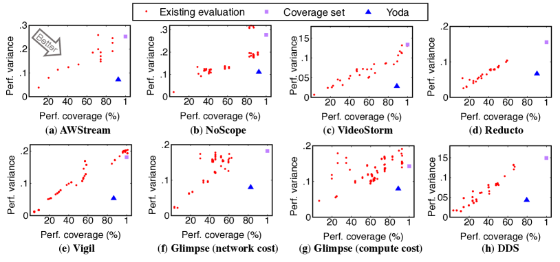
Figure 9. Yoda achieves a much higher level of performance clarity (higher coverage and lower variance), compared to existing evaluation methods. A high coverage means Yoda reveals both good and bad performance of a VAP, whereas a low variance means Yoda accurately estimates a VAP’s performance on new videos.

5.3. YODA’s Workflow

Using the proposed primitive-based profiling, Yoda offers two key functions for its users: VAP profiler that produces a PC profile $\mathbb{P}_{v}$ for each VAP $v$, and VAP performance estimator that directly estimates $v$’s performance on a target video using $\mathbb{P}_{v}$ without the need to run $v$ on the video.

In the following, we use $v=(t,s,m)$ to denote a VAP, with $t,s$ and $m$ being its temporal-pruning strategy, spatial-pruning strategy, and model-pruning strategy, respectively. The PC profile of $v=(t,s,m)$ is a lookup table $\mathbb{P}_{v}$ (or $\mathbb{P}_{t,s,m}$) that maps a feature value combination $x$ in the feature space of $\mathbb{F}$ to the expected performance in accuracy and cost $\mathbb{P}_{t,s,m}(x)$.

VAP profiler:  Leveraging the property of cross-primitive independence (§5.1), Yoda builds the PC profile of $v=(t,s,m)$ in two steps. First, we build a per-primitive profile of each of its strategies. The temporal-pruning profile of $v$, for instance, is $\mathbb{P}_{t,s^{*},m^{*}}$, where $t^{*},s^{*}$ and $m^{*}$ denote the oracle strategies (see §5.1) of temporal pruning, spatial pruning and model pruning, respectively. That is, we build $\mathbb{P}_{t,s^{*},m^{*}}$ by setting $v$’s spatial and model pruning strategies to their oracle ones and testing it on the benchmark videos for temporal pruning (introduced in §5.2). Second, we build the full PC profile as

(1) $$\mathbb{P}_{t,s,m}(x)=\mathbb{P}_{t,s^{*},m^{*}}(x)\cdot\mathbb{P}_{t^{*},s,m^{*}}(x)\cdot\mathbb{P}_{t^{*},s^{*},m}(x)$$

VAP performance estimator:  In practice, operators often need to estimate a VAP’s performance on a new (long) video. The challenge is that naive featurization will require annotating every object (by human annotation or running a full DNN), which can be painstakingly slow. Fortunately, obtaining the distribution of feature values over an entire video does not require accurate results on each single frame. Instead, we show that running a low-cost object detector (e.g., MobileNet-SSD) on aggressively sampled frames can still yield reliable estimate of the overall feature value distribution. For instance, to get the distribution of per-object area, we run Mobilenet-SSD on 10x uniformly sampled frames to get the area of each detected object and use the distribution of these areas as the result. This way, Yoda can quickly scan a long video and produce reliable estimation of the distribution of each feature value. Once the feature distribution is known, Yoda then uses $\mathbb{P}_{v}$ to directly map the feature value distribution to $v$’s performance on the video.

We implement Yoda as a ready-to-use toolkit for profiling and evaluating VAPs, and plan to release the toolkit to the research community. The toolkit provides a shared library (API) for emulating and benchmarking VAPs.

6. Evaluation

We evaluate the efficacy of Yoda in achieving VAP performance clarity. Specifically, we conduct experiments to answer the following questions:

• Does Yoda achieve higher VAP performance clarity, compared to existing solutions that emprically test VAPs on a corpus of videos? (§6.1)

• Is Yoda’s primitive-based profiling accurate and efficient? Can it generalize to new VAPs? (§6.2)

• Can Yoda accurately predict a VAP’s performance on new videos at a low computation cost? (§6.3)

• Does Yoda provide new insights for VAP design and deployment? (§6.4)

6.1. Yoda’s Performance Clarity

As defined in §4.1, performance clarity aims at providing a comprehensive characterization of VAP performance. Here, we measure the level of achieved performance clarity by two dimensions: coverage (the completeness of the evaluation, the higher the better) and variance (the ambiguity of the evaluation outcome, the lower the better). The intuition is that an ideal VAP performance evaluation should have high performance coverage and low variance. A high coverage means Yoda reveals both good and bad performance of a VAP, whereas a low variance means Yoda accurately estimates a VAP’s performance on new videos. The specific metrics of coverage and variance are defined as follows. Given a VAP $v$’s PC profile $\mathbb{P}_{v}$ (measured from our benchmark dataset of 67-minute videos), Yoda first uses $\mathbb{P}_{v}$ to estimate $v$’s cost at a specific accuracy range ([0.9,0.95]) for all videos in the coverage dataset excluding our benchmark videos. Then, we compute Yoda’s coverage as the observed cost value range, normalized by the observed cost value range when testing $v$ on the whole coverage dataset (14.5 hours of videos). Next, we compute the standard deviation of Yoda’s cost values as Yoda’s variance. Figure 9 shows the results of 7 pipelines in the blue boxes: Yoda achieves high coverage ($>$90%) and low variance ($<$0.2). The figures show one scenario per VAP, but the conclusion holds in other scenarios.

Yoda vs. existing methods:  Figure 9 also compares the (coverage, variance) results from the traditional evaluation method, which tests the performance on a long video (or a set of videos) from the target scenario (represented by the red dots). For fairness, each test video is no shorter than our benchmark video. We see that the coverage fluctuates significantly across videos and the variance per video is much higher. This confirms that traditional evaluations lead to either incomplete/partial conclusions or ambiguous results (as we have shown in §3.2). As a reference point, when the traditional evaluation uses the entire coverage dataset (14.5 hours), the variance exceeds 0.25, again significantly larger than Yoda.

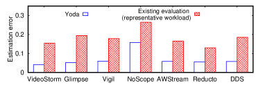
Figure 10. Yoda provides more accurate estimation of VAP performance on new videos than traditional profiling using representative workload per scenario.

Microscopic study on VAP performance estimation:  We take a further step to examine the benefit of elevated performance clarity, using the task of per-video VAP performance estimation. Given Yoda’s $\mathbb{P}_{v}$, we directly estimate a VAP $v$’s performance on any video, and compare it to the ground truth result obtained by running $v$ on the video. Again we keep the accuracy to [0.9,0.95] and measure the absolute difference between the cost value predicted by $\mathbb{P}_{v}$ and the ground truth, which we refer to as cost “estimation error”. As reference, we apply an “ traditional profiler” to estimate $v$’s cost in the same accuracy range by running $v$ on a representative long workload under the same scenario of the test video, and compare it against the ground truth.

Figure 10 plots the median estimation errors of both Yoda’s profiler and the traditional profiler, across all the long videos in the coverage dataset (that are not used for profiling). We see that Yoda’s profiler is much more accurate than the traditional profiler at estimating VAP performance on new videos.

6.2. Primitive-based Profiling: Accuracy, Cost, and Generality

Yoda’s efficiency partly stems from its primitive-based profiling, which tests a VAP on only videos that vary along the primitive-related features. To evaluate it, we compare Yoda with an expensive profiler built on the whole coverage set.

Accuracy:  We measure the discrepancy between the PC profile built on the whole coverage set and Yoda’s PC profile. The average differences between the profiled performance curves (cost differences at same accuracy levels) are listed in Table 8 for each of the seven VAPs, and are all very low. This corroborates our intuition in §5.2 that a small subset of videos is sufficient to profile PC, since the feature distribution in the coverage set is highly uneven.

Profiling cost:  Profiling a VAP is a one-time cost (i.e., no need to repeat unless the VAP changes its design). The computation cost of profiling depends on the VAP design. Intuitively, VAPs that do not optimize/reduce compute cost will incur a higher overhead. Thus we present the result of AWStream, a VAP that does not optimize for compute cost. To profile AWStream, Yoda needs to run the VAP process on $\sim$72k frames using the full DNN model for object detection, at four different video quality levels and twelve different frame sampling rates. When running on an Amazon EC2 machine (instance p2.16xlarge that has 16 GPUs and costs $14.4/hr), the profiling takes 8.5 minutes and cost $2. Even a VAP, such as VideoStorm, that needs to profile all three primitives takes only 22.2 minutes and cost $5.3.

	Glimpse	Vigil	VideoStorm	AWStream	NoScope	Reducto	DDS
Profile diff (Yoda vs. coverage set)	0.043	0.005	0.048	0.063	0.083	0.030	0.058

Table 8. Discrepancy between the PC profile built on Yoda selected videos and the PC profile built on coverage set videos.

Generality:  Can Yoda accurately profile a new VAP not considered by Yoda’s feature and benchmark video selection process? As mentioned earlier, we intentionally held out three of the seven VAPs (AWStream, Reducto, and DDS) from the feature/video selection process (§5.2). Nonetheless, Figures 9 & 10 and Table 8 show that Yoda achieve similar profiling effectiveness on these holdout VAPs as on other VAPs. While this does not prove that Yoda generalizes to all future VAPs, it does indicates that Yoda might profile new VAPs as accurately as the other VAPs used in its feature selection process.

6.3. Fast-yet-accurate Performance Estimation

Recall that Yoda offers a useful function of directly estimating a VAP $v$’s performance on any video, without running $v$ on the video. We have validated the quality of performance estimation in Figure 10 (§6.1), using the task of estimating cost at a specific accuracy range ([0.9,0.95]). Below we provide more results on its estimation accuracy and computation cost.

We consider the task to understand the variability of VAP accuracy throughout a target video. For this we define two metrics on accuracy variability: (1) fraction of video segments whose accuracy is above 0.85, denoted by $\alpha$; and (2) fraction of video segments whose accuracy is below 0.7, denoted by $\beta$. Such metrics are useful in practice since operators often need to maintain accuracy at an acceptable level. We use the accuracy distribution of actually running the VAP on the video as the ground truth and define the estimation error by $|\alpha_{estimated}-\alpha_{real}|$ and $|\beta_{estimated}-\beta_{real}|$.

We also evaluate Yoda against a “resource friendly” baseline that actually runs $v$ on a sample set of video frames, whose estimation accuracy and overhead depend on the sampling rate. Note that as explained in §5.3, Yoda’s performance estimator also needs to scan a sample set of video frames to measure the video’s feature value distribution. Thus its accuracy and overhead also vary with the sampling rate.

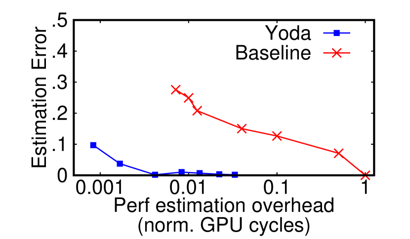
(a) Estimating VideoStorm’s fraction of high accuracy ($\alpha$)

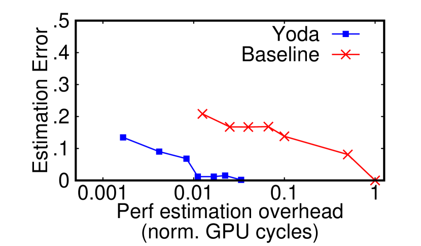
(b) Estimating VideoStorm’s fraction of low accuracy ($\beta$)

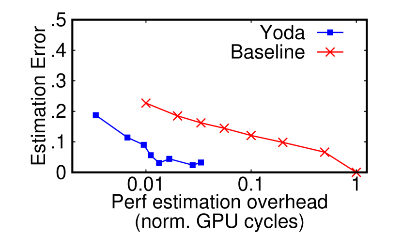
(c) Estimating AWStream’s fraction of high accuracy ($\alpha$)

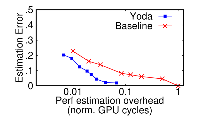
(d) Estimating AWStream’s fraction of low accuracy ($\beta$)

Figure 11. Yoda estimates VAP performance faster and more accurately than actually running VAP on the test videos.

Figure 11 shows the estimation errors of Yoda and baseline on VideoStorm and AWStream, as a function of the estimation overhead (amount of GPU cycles consumed), for 5 hours of dashcam videos (not used during profiling). Here Yoda uses MobileNet-SSD (google-model-zoo, ) as the cheap object detector to scan the videos. For clarity, we normalize the estimation overhead by the amount of GPU cycles consumed by running each VAP on the full video. We see that Yoda achieves nearly perfect estimation at a much lower cost, i.e., nearly 2 orders of magnitude faster than running the VAP on the video.

6.4. Practical Insights for VAP Deployment

By providing a comprehensive profiling on VAP performance, Yoda also identifies new insights for guiding VAP design and deployment. We highlight two concrete use cases here.

Conditional correlations among features:  Figure 12 shows the performance of Glimpse’s temporal pruning strategy against two features: $x_{1}$ (% of frames with objects) and $x_{2}$ (average object speed). For better visualization, we only show the minimum cost while maintaining accuracy over 0.9 (i.e., a slice of the cost-accuracy tradeoff). Figure 12(a) and (b) show that both compute and network costs are strongly correlated with $x_{1}$ when $x_{2}$ is over 1.6 (which is a typical vehicle speed in highway videos). But when $x_{2}$ is below 1.6 (Figure 12(c)), the correlation becomes remarkably weaker.

This result implies that when testing VAPs that use this pruning strategy (e.g., NoScope, Glimpse), the traditional method may either miss this correlation (if most test videos have slow moving objects) or claim a strong correlation (if most test videos have fast moving objects). In contrast, Yoda reveals not only both correlation patterns, but also when they emerge, which helps to decide if a VAP should be deployed in certain video content.

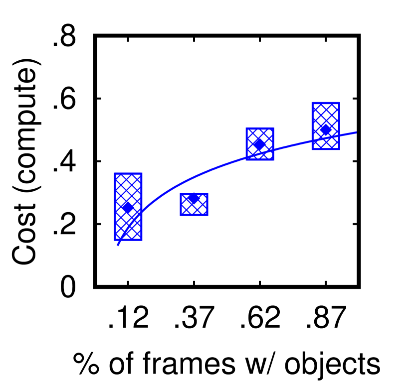
(a) Compute cost v.s. $x_{1}$ when $x_{2}$ >= 1.6.

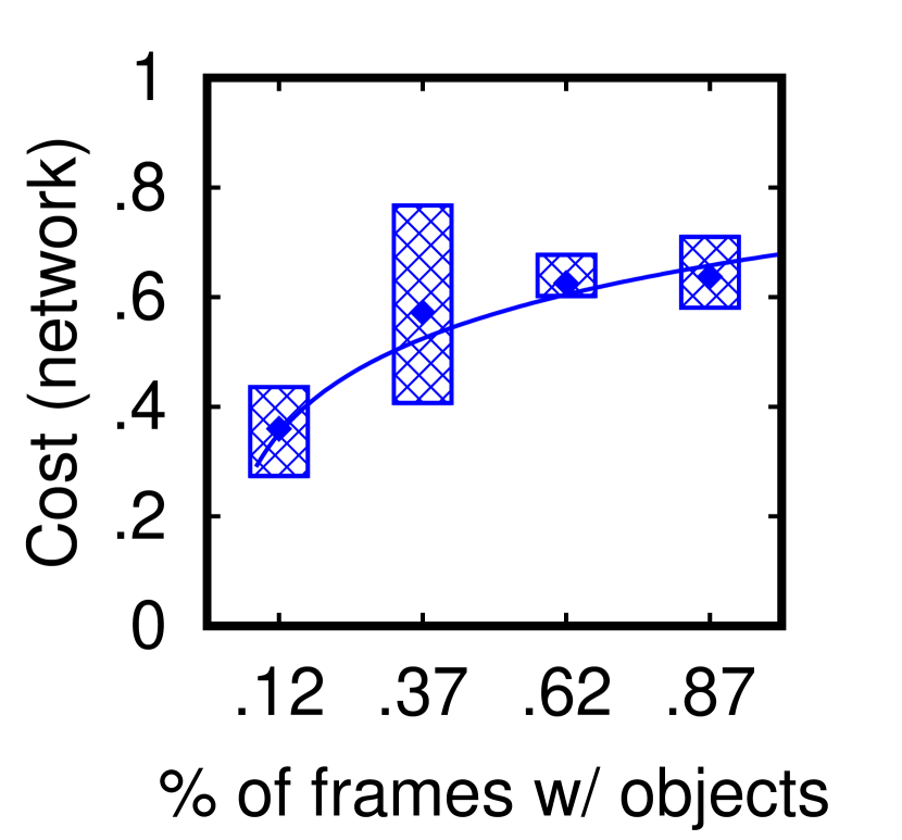
(b) Network cost v.s. $x_{1}$ when $x_{2}$ >= 1.6.

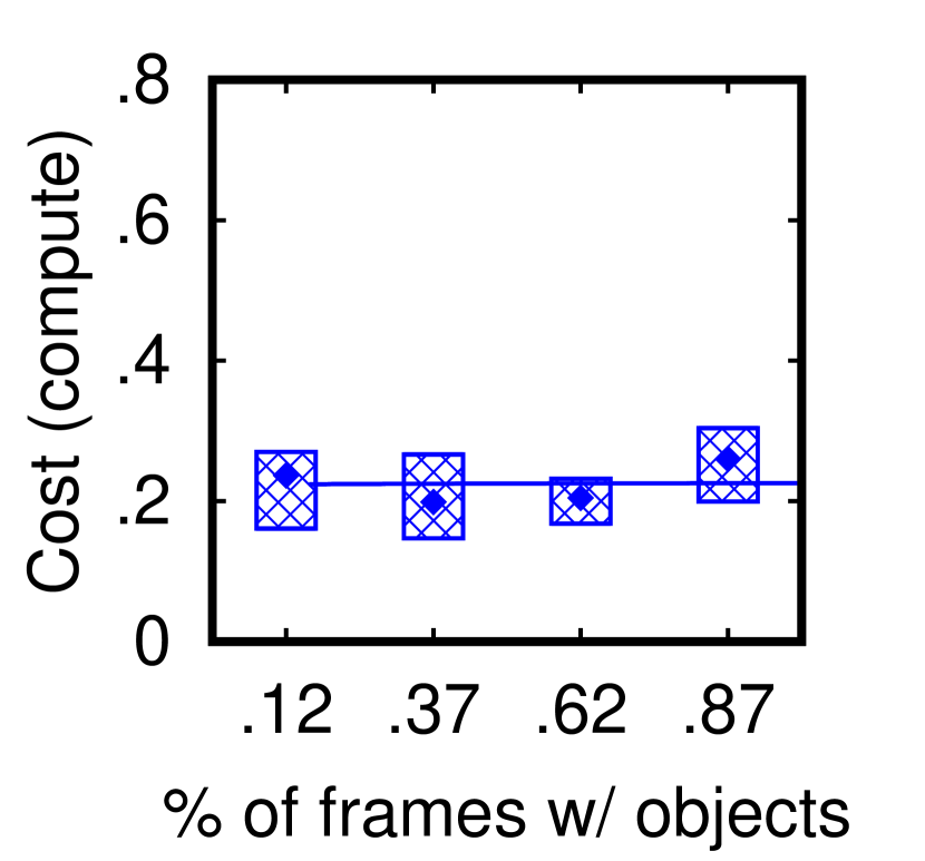
(c) Compute cost v.s. $x_{1}$ when $x_{2}$ < 1.6.

Figure 12. Impact of feature $x_{1}$ (% of frames with objects) on performance depends on the value of feature $x_{2}$ (avg. object speed). Each box shows the mean and 25${}^{\textrm{th}}$ and 75${}^{\textrm{th}}$ %iles.

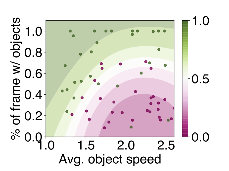
(a) Temporal pruning: Uniform vs. frame diff-triggered selection

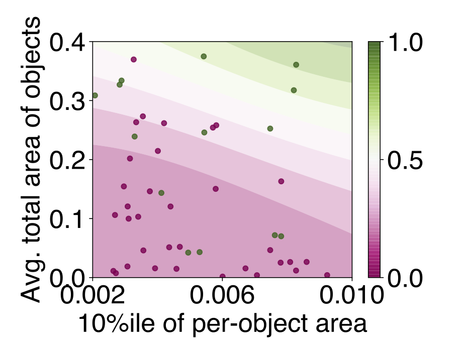
(b) Spatial pruning: Image quality downsizing vs. region cropping

Figure 13. In both primitives, there is no single strategy that fits in all type of content. The coloring indicates that where one strategy is likely better than the other.

Informed choices of VAP strategies:  As a case study, let us consider two temporal-pruning strategies (uniform frame selection vs. frame difference-triggered frame selection) and two spatial-pruning strategies (image quality downsizing vs. image region cropping). Figure 13(a) shows the operating regime of each temporal-pruning strategy: frame difference-triggered selection is better when only a small fraction of frames contain objects and these objects move fast (magenta). Otherwise, uniform frame sampling is better (green). Similarly, Figure 13(b) shows that image quality downsizing is likely to be better if the objects are large and occupy more space in frames (green), and otherwise the image cropping strategy is better (magenta). These differences stem from how various strategies interact with videos. For instance, image quality downsizing eliminates redundant pixels in large objects of interest (which can be detected with less pixels), whereas image cropping eliminates redundant pixels outside of objects of interest by subtracting background.

These results have significant practical implications. For instance, for urban traffic videos during peak hours, AWStream (uniform frame sampling and image downsizing) is better than Glimpse (frame difference-triggered frame selection), because the vehicles appear frequently and in large numbers and move slowly and often in relatively big sizes (crossroad cameras tend to be closer to the road than highway cameras), so it falls in the green regions of both graphs. In contrast, for urban traffic videos during off-peak hours, where many large-size objects move quickly (i.e., magenta in Figure 13(a) and green in Figure 13(b)), we should create a new VAP that combines Glimpse’s temporal-pruning strategy and AWStream’s spatial pruning strategy.

7. Related work

Video analytics pipelines:  Besides the VAPs described in §2, there are other VAPs that utilize the same three primitives: temporal pruning (e.g., (eaar, ; emo, ; clownfish, ; scaling, ; wang2018bandwidth, ; deepdecision, )), spatial pruning (e.g., (eaar, ; grace, ; catdet, ; deepdecision, )) and model pruning (e.g., (nestdnn, ; clownfish, ; approxdet, ; resolution, ; deepdecision, )). Some work also reduces the compute/communication cost of computer-vision inference pipelines, through super resolution (e.g., (cloudseg, ; shermeyer2019effects, ; adascale, )), splitting the DNN between camera and server (e.g., (rexcam-hotmobile, ; ddnn, ; mcdnn, ; emmons2019cracking, ; hsu2019couper, )), DNN-aware cloud/edge resource scheduling (e.g., (mcdnn, ; blazeit, ; hotnets, ; e2m, ; distream, )), cross-camera or cross-application correlations (e.g., (amvp, ; spatula, ; distream, ; liu2019caesar, ; kestrel, )), scalable data management and execution frameworks (e.g., (optasia, ; deeplens-sanjay, ; scanner, ; edgeeye, )), and DNN architectures tailored to balance throughput and accuracy (e.g., (yolov3, ; huang2017multi, ; bolukbasi2017adaptive, ; wang2018skipnet, ; tsm, ; mainstream, ; flexdnn, )). Many of these techniques leverage content-level characteristics, such as the ones we have discussed. We hope that by revealing the importance (and feasibility) of PC, future work can extend Yoda to support these VAPs. While a few prior works have mentioned the issue of performance variability on some VAPs, the results were limited and only based on a handful of video features (e.g., object size (dds-sigcomm, )). To the best of our knowledge, our work is the first to systematically study (using measurements & building benchmarks) how video content features affect VAP performances.

Edge/video analytics benchmarks:  Several benchmarks of video analytics systems have been proposed for various focuses, including throughput of video database (e.g., (visual-road, ; scanner, )), video encoding efficiency (e.g., (xiph, ; vbench, )), and shared library to implement video inference pipelines (e.g., (rocket, )). More general benchmarks catered for edge network environments are proposed as well (benchmarkingTinyML, ; defog, ; kolosov2020benchmarking, ). Also related to Yoda are those benchmarking vision-task accuracies (e.g., (kitti, ; dukemtmc, )) and their tradeoffs with throughput/latency (e.g., (google-benchmark, )). While most benchmarks focus on average performance across images/videos, some did observe that vision models perform differently across content (objectnet, ) and can be sensitive to video encoding (hendrycks2019benchmarking, ) or training data quality (zhao2020role, ). Yoda takes one step further to systematically reveal the influence of video content features on VAP performance. Recent efforts in computer vision similarly demonstrate that features of the test data affect the performance of a classification model (e.g., (balaji2019instance, ; gebru2017fine, )), though they focus on perturbing the features to improve model robustness whereas Yoda seeks to reveal the hidden relationship between VAP performance and content features.

Traditionally, the systems community has benefited from thorough performance benchmarking of data analytics systems under a wide range of workloads (e.g., (armstrong2013linkbench, ; ycsb, )), and our work is one example of this line of work in the context of video analytics.

8. Conclusion

Our work is a response to the recent trend of building efficient mobile video analytics systems, at the expense of significant performance variability caused by video content dependency. We present a measurement study to shed light on this issue for the first time, and propose the first VAP benchmark that elevates performance clarity (how video content affects performance). Although Yoda only scratches the surface of VAP performance clarity, it is shown to be effective and capable of identifying hidden design tradeoffs.

- (1) Ai traffic video analytics platform being developed. https://www.traffictechnologytoday.com/news/traffic-management/ai-traffic-video-analytics-platform-being-developed.html.
- (2) At&t unlimited data plans with talk & text. https://www.att.com/plans/unlimited-data-plans/. (Accessed on 06/15/2020).
- (3) British transport police: Cctv. http://www.btp.police.uk/advice_and_information/safety_on_and_near_the_railway/cctv.aspx. Accessed: 2018-10-27.
- (4) Can 30,000 cameras help solve chicago’s crime problem? https://www.nytimes.com/2018/05/26/us/chicago-police-surveillance.html. Accessed: 2018-10-27.
- (5) Can physical distance monitoring & smart cameras help businesses reopen faster? https://www.wwt.com/article/can-physical-distance-monitoring-and-smart-cameras-help-businesses-reopen-faster.
- (6) Duke mtmc (multi-target, multi-camera). https://megapixels.cc/duke_mtmc/.
- (7) Goodvision: Smart traffic data analytics. https://goodvisionlive.com/.
- (8) A guide to video analytics: Applications and opportunities. https://tryolabs.com/resources/video-analytics-guide/.
- (9) Humans can’t watch all the surveillance cameras out there, so computers are. https://slate.com/technology/2019/06/video-surveillance-analytics-software-artificial-intelligence-dangerous.html. Accessed: 2019-3-4.
- (10) intuvision va traffic use case. https://www.intuvisiontech.com/intuvisionVA_solutions/intuvisionVA_traffic.
- (11) Microsoft rocket video analytics platform. https://github.com/microsoft/Microsoft-Rocket-Video-Analytics-Platform.
- (12) Smart retail, digital transformation of retail business. https://gyrus.ai/blog/smart-retail-location-point-of-sale-analytics-camera/.
- (13) Tensorflow detection model zoo. https://github.com/tensorflow/models/blob/master/research/object_detection/g3doc/detection_model_zoo.md.
- (14) Traffic video analytics – case study report. https://www.microsoft.com/en-us/research/publication/traffic-video-analytics-case-study-report/.
- (15) Trafficvision: Traffic intelligence from video. http://www.trafficvision.com/.
- (16) Video analytics for public health use cases. https://www.briefcam.com/video-analytics-for-public-health-use-cases/.
- (17) Video analytics market size worth $9.4 billion by 2025 | cagr: 22.8%. https://www.grandviewresearch.com/press-release/global-video-analytics-market. Accessed: 2019-2-13.
- (18) The vision zero initiative. http://www.visionzeroinitiative.com/. Accessed: 2019-3-1.
- (19) Vision zero video analytics partnerships. https://bellevuewa.gov/city-government/departments/transportation/safety-and-maintenance/traffic-safety/vision-zero/video-analytics.
- (20) Xiph.org video test media. https://media.xiph.org/video/derf/.
- (21) Data generated by new surveillance cameras to increase exponentially in the coming years. http://www.securityinfowatch.com/news/12160483/, 2016.
- (22) Armstrong, T. G., Ponnekanti, V., Borthakur, D., and Callaghan, M. Linkbench: a database benchmark based on the facebook social graph. In Proc. of SIGMOD (2013).
- (23) Balaji, Y., Goldstein, T., and Hoffman, J. Instance adaptive adversarial training: Improved accuracy tradeoffs in neural nets. arXiv preprint arXiv:1910.08051 (2019).
- (24) Banbury, C. R., Reddi, V. J., Lam, M., Fu, W., Fazel, A., Holleman, J., Huang, X., Hurtado, R., Kanter, D., Lokhmotov, A., et al. Benchmarking tinyml systems: Challenges and direction. Proc. of MLsys workshop (2020).
- (25) Barbu, A., Mayo, D., Alverio, J., Luo, W., Wang, C., Gutfreund, D., Tenenbaum, J., and Katz, B. Objectnet: A large-scale bias-controlled dataset for pushing the limits of object recognition models. In Proc. of NeurIPS (2019).
- (26) Bolukbasi, T., Wang, J., Dekel, O., and Saligrama, V. Adaptive neural networks for efficient inference. In Proc. of ICML (2017), vol. 70.
- (27) Canel, C., Kim, T., Zhou, G., Li, C., Lim, H., Andersen, D. G., Kaminsky, M., and Dulloor, S. R. Scaling video analytics on constrained edge nodes.
- (28) Chao, M., Stoleru, R., Jin, L., Yao, S., Maurice, M., and Blalock, R. Amvp: Adaptive cnn-based multitask video processing on mobile stream processing platforms. In Proc. of ACM/IEEE Symposium on Edge Computing (SEC) (2020).
- (29) Chen, J., and Ran, X. Deep learning with edge computing: A review. Proceedings of the IEEE 107 (2019).
- (30) Chen, T. Y.-H., Ravindranath, L., Deng, S., Bahl, P., and Balakrishnan, H. Glimpse: Continuous, real-time object recognition on mobile devices. In Proc. of Sensys (2015).
- (31) Chin, T.-W., Ding, R., and Marculescu, D. Adascale: Towards real-time video object detection using adaptive scaling.
- (32) Coleman, C., Kang, D., Narayanan, D., Nardi, L., Zhao, T., Zhang, J., Bailis, P., Olukotun, K., Ré, C., and Zaharia, M. Analysis of dawnbench, a time-to-accuracy machine learning performance benchmark. ACM SIGOPS Operating Systems Review 53 (2019).
- (33) Coleman, C., Narayanan, D., Kang, D., Zhao, T., Zhang, J., Nardi, L., Bailis, P., Olukotun, K., Ré, C., and Zaharia, M. Dawnbench: An end-to-end deep learning benchmark and competition. Training 100 (2017).
- (34) Cooper, B. F., Silberstein, A., Tam, E., Ramakrishnan, R., and Sears, R. Benchmarking cloud serving systems with ycsb. In Proc. of SoCC (2010).
- (35) Deng, J., Dong, W., Socher, R., Li, L.-J., Li, K., and Fei-Fei, L. Imagenet: A large-scale hierarchical image database. In Proc. of CVPR (2009).
- (36) Du, K., Pervaiz, A., Yuan, X., Chowdhery, A., Zhang, Q., Hoffmann, H., and Jiang, J. Server-driven video streaming for deep learning inference. In Proc. of SIGCOMM (2020).
- (37) Emmons, J., Fouladi, S., Ananthanarayanan, G., Venkataraman, S., Savarese, S., and Winstein, K. Cracking open the dnn black-box: Video analytics with dnns across the camera-cloud boundary. In Proc. of HotEdgeVideo (2019).
- (38) Everingham, M., Van Gool, L., Williams, C. K., Winn, J., and Zisserman, A. The pascal visual object classes (voc) challenge. International journal of computer vision 88 (2010).
- (39) Fang, B., Zeng, X., Zhang, F., Xu, H., and Zhang, M. Flexdnn: Input-adaptive on-device deep learning for efficient mobile vision. In Proc. of ACM/IEEE Symposium on Edge Computing (SEC) (2020).
- (40) Fang, B., Zeng, X., and Zhang, M. Nestdnn: Resource-aware multi-tenant on-device deep learning for continuous mobile vision. In Proc. of Mobicom (2018).
- (41) Gebru, T., Hoffman, J., and Fei-Fei, L. Fine-grained recognition in the wild: A multi-task domain adaptation approach. In Proc. of ICCV (2017).
- (42) Geiger, A., Lenz, P., and Urtasun, R. Are we ready for autonomous driving? the kitti vision benchmark suite. In Proc. of CVPR (2012).
- (43) Geiger, A., Lenz, P., and Urtasun, R. Are we ready for autonomous driving? the kitti vision benchmark suite. In Proc. of CVPR (2012).
- (44) Han, S., Shen, H., Philipose, M., Agarwal, S., Wolman, A., and Krishnamurthy, A. Mcdnn: An approximation-based execution framework for deep stream processing under resource constraints. In Proc. of Mobisys (2016).
- (45) Haynes, B., Mazumdar, A., Balazinska, M., Ceze, L., and Cheung, A. Visual road: A video data management benchmark. In Proc. of SIGMOD (2019).
- (46) Hendrycks, D., and Dietterich, T. Benchmarking neural network robustness to common corruptions and perturbations. arXiv preprint arXiv:1903.12261 (2019).
- (47) Hsu, K.-J., Bhardwaj, K., and Gavrilovska, A. Couper: Dnn model slicing for visual analytics containers at the edge. In Proc. of ACM/IEEE Symposium on Edge Computing (SEC) (2019).
- (48) Huang, G., Chen, D., Li, T., Wu, F., van der Maaten, L., and Weinberger, K. Q. Multi-scale dense networks for resource efficient image classification. arXiv preprint arXiv:1703.09844 (2017).
- (49) Huang, J., Rathod, V., Sun, C., Zhu, M., Korattikara, A., Fathi, A., Fischer, I., Wojna, Z., Song, Y., Guadarrama, S., et al. Speed/accuracy trade-offs for modern convolutional object detectors. In Proc. of CVPR (2017).
- (50) Hung, C.-C., Ananthanarayanan, G., Bodik, P., Golubchik, L., Yu, M., Bahl, V., and Philipose, M. Videoedge: Processing camera streams using hierarchical clusters. In Proc. of ACM/IEEE Symposium on Edge Computing (SEC) (2018).
- (51) Jain, S., Ananthanarayanan, G., Jiang, J., Shu, Y., and Gonzalez, J. Scaling video analytics systems to large camera deployments. In Proc. of HotMobile (2019).
- (52) Jain, S., Zhang, X., Zhou, Y., Ananthanarayanan, G., Jiang, J., Shu, Y., Bahl, P., and Gonzalez, J. Spatula: Efficient cross-camera video analytics on large camera networks.
- (53) Jiang, A. H., Wong, D. L.-K., Canel, C., Tang, L., Misra, I., Kaminsky, M., Kozuch, M. A., Pillai, P., Andersen, D. G., and Ganger, G. R. Mainstream: Dynamic stem-sharing for multi-tenant video processing. In Proc. of USENIX ATC (2018).
- (54) Jiang, J., Ananthanarayanan, G., Bodik, P., Sen, S., and Stoica, I. Chameleon: scalable adaptation of video analytics. In Proc. of SIGCOMM (2018).
- (55) Kang, D., Bailis, P., and Zaharia, M. Blazeit: optimizing declarative aggregation and limit queries for neural network-based video analytics. Proc. of VLDB 13 (2019).
- (56) Kang, D., Emmons, J., Abuzaid, F., Bailis, P., and Zaharia, M. Noscope: optimizing neural network queries over video at scale. In Proc. of VLDB (2017).
- (57) Kolosov, O., Yadgar, G., Maheshwari, S., and Soljanin, E. Benchmarking in the dark: On the absence of comprehensive edge datasets. In Proc. of USENIX Workshop on Hot Topics in Edge Computing (HotEdge) (2020).
- (58) Krishnan, S., Dziedzic, A., and Elmore, A. J. Deeplens: Towards a visual data management system. arXiv preprint arXiv:1812.07607 (2018).
- (59) Li, Y., Padmanabhan, A., Zhao, P., Wang, Y., Xu, H., and Netravali, R. Reducto: On-camera filtering for resource-efficient real-time video analytics. In Proc. of SIGCOMM (2020).
- (60) Lin, J., Gan, C., and Han, S. Tsm: Temporal shift module for efficient video understanding. In Proc. of ICCV (2019).
- (61) Lin, T.-Y., Maire, M., Belongie, S., Hays, J., Perona, P., Ramanan, D., Dollár, P., and Zitnick, C. L. Microsoft coco: Common objects in context. In Proc. of ECCV (2014).
- (62) Liu, L., Chen, J., Brocanelli, M., and Shi, W. E2m: an energy-efficient middleware for computer vision applications on autonomous mobile robots. In Proc. of ACM/IEEE Symposium on Edge Computing (SEC) (2019).
- (63) Liu, L., Li, H., and Gruteser, M. Edge assisted real-time object detection for mobile augmented reality. In Proc. of Mobicom (2019).
- (64) Liu, P., Qi, B., and Banerjee, S. Edgeeye: An edge service framework for real-time intelligent video analytics. In Proc. of International Workshop on Edge Systems, Analytics and Networking (2018).
- (65) Liu, X., Ghosh, P., Ulutan, O., Manjunath, B., Chan, K., and Govindan, R. Caesar: cross-camera complex activity recognition. In Proc. of Sensys (2019).
- (66) Lottarini, A., Ramirez, A., Coburn, J., Kim, M. A., Ranganathan, P., Stodolsky, D., and Wachsler, M. vbench: Benchmarking video transcoding in the cloud. In ACM SIGPLAN Notices (2018), vol. 53.
- (67) Lu, Y., Chowdhery, A., and Kandula, S. Optasia: A relational platform for efficient large-scale video analytics. In Proc. of SoCC (2016), ACM.
- (68) Mao, H., Kong, T., and Dally, W. J. Catdet: Cascaded tracked detector for efficient object detection from video.
- (69) McChesney, J., Wang, N., Tanwer, A., de Lara, E., and Varghese, B. Defog: fog computing benchmarks. In Proc. of ACM/IEEE Symposium on Edge Computing (SEC) (2019).
- (70) Milan, A., Leal-Taixé, L., Reid, I., Roth, S., and Schindler, K. MOT16: A benchmark for multi-object tracking. arXiv:1603.00831 (2016).
- (71) Mukaka, M. M. A guide to appropriate use of correlation coefficient in medical research. Malawi medical journal 24 (2012).
- (72) Mullapudi, R. T., Chen, S., Zhang, K., Ramanan, D., and Fatahalian, K. Online model distillation for efficient video inference. In Proc. of ICCV (2019).
- (73) Nigade, V., Wang, L., and Bal, H. Clownfish: Edge and cloud symbiosis for video stream analytics. In Proc. of ACM/IEEE Symposium on Edge Computing (SEC) (2020).
- (74) Noghabi, S. A., Cox, L., Agarwal, S., and Ananthanarayanan, G. The emerging landscape of edge computing. GetMobile: Mobile Computing and Communications 23 (2020).
- (75) P. Chinchali, S., Cidon, E., Pergament, E., Chu, T., and Katti, S. Neural networks meet physical networks: Distributed inference between edge devices and the cloud. In Proc. of HotNets (2018).
- (76) Pakha, C., Chowdhery, A., and Jiang, J. Reinventing video streaming for distributed vision analytics. In Proc. of HotCloud (2018).
- (77) Poms, A., Crichton, W., Hanrahan, P., and Fatahalian, K. Scanner: Efficient video analysis at scale. ACM Transactions on Graphics (TOG) 37 (2018).
- (78) Qiu, H., Liu, X., Rallapalli, S., Bency, A. J., Chan, K., Urgaonkar, R., Manjunath, B., and Govindan, R. Kestrel: Video analytics for augmented multi-camera vehicle tracking. In Proc. of International Conference on Internet-of-Things Design and Implementation (IoTDI) (2018).
- (79) Ran, X., Chen, H., Zhu, X., Liu, Z., and Chen, J. Deepdecision: A mobile deep learning framework for edge video analytics. In Proc. of INFOCOM (2018).
- (80) Redmon, J., and Farhadi, A. Yolov3: An incremental improvement. arXiv (2018).
- (81) Shen, H., Han, S., Philipose, M., and Krishnamurthy, A. Fast video classification via adaptive cascading of deep models. In Proc. of CVPR (2017).
- (82) Shermeyer, J., and Van Etten, A. The effects of super-resolution on object detection performance in satellite imagery. In Proc. of CVPR Workshops (2019).
- (83) Sun, P., Kretzschmar, H., Dotiwalla, X., Chouard, A., Patnaik, V., Tsui, P., Guo, J., Zhou, Y., Chai, Y., Caine, B., Vasudevan, V., Han, W., Ngiam, J., Zhao, H., Timofeev, A., Ettinger, S., Krivokon, M., Gao, A., Joshi, A., Zhang, Y., Shlens, J., Chen, Z., and Anguelov, D. Scalability in perception for autonomous driving: Waymo open dataset. In Proc. of CVPR (2019).
- (84) Teerapittayanon, S., McDanel, B., and Kung, H. Distributed deep neural networks over the cloud, the edge and end devices. In Proc. of ICDCS (2017).
- (85) Wang, J., Feng, Z., Chen, Z., George, S., Bala, M., Pillai, P., Yang, S.-W., and Satyanarayanan, M. Bandwidth-efficient live video analytics for drones via edge computing. In Proc. of ACM/IEEE Symposium on Edge Computing (SEC) (2018).
- (86) Wang, X., Yu, F., Dou, Z.-Y., Darrell, T., and Gonzalez, J. E. Skipnet: Learning dynamic routing in convolutional networks. In Proc. of ECCV (2018).
- (87) Wang, Y., Wang, W., Zhang, J., Jiang, J., and Chen, K. Bridging the edge-cloud barrier for real-time advanced vision analytics. In Proc. of HotCloud (2019).
- (88) Wu, H., Feng, J., Tian, X., Sun, E., Liu, Y., Dong, B., Xu, F., and Zhong, S. Emo: Real-time emotion recognition from single-eye images for resource-constrained eyewear devices. In Proc. of Mobisys (2020).
- (89) Xie, X., and Kim, K.-H. Source compression with bounded dnn perception loss for iot edge computer vision. In Proc. of Mobicom (2019).
- (90) Xu, R., Zhang, C.-l., Wang, P., Lee, J., Mitra, S., Chaterji, S., Li, Y., and Bagchi, S. Approxdet: content and contention-aware approximate object detection for mobiles. In Proc. of Sensys (2020).
- (91) Yang, L., Han, Y., Chen, X., Song, S., Dai, J., and Huang, G. Resolution adaptive networks for efficient inference. In Proc. of CVPR (2020).
- (92) Zeng, X., Fang, B., Shen, H., and Zhang, M. Distream: scaling live video analytics with workload-adaptive distributed edge intelligence. In Proc. of Sensys (2020).
- (93) Zhang, B., Jin, X., Ratnasamy, S., Wawrzynek, J., and Lee, E. A. Awstream: adaptive wide-area streaming analytics. In Proc. of SIGCOMM (2018).
- (94) Zhang, H., Ananthanarayanan, G., Bodik, P., Philipose, M., Bahl, P., and Freedman, M. J. Live video analytics at scale with approximation and delay-tolerance. In Proc. of NSDI (2017).
- (95) Zhang, T., Chowdhery, A., Bahl, P. V., Jamieson, K., and Banerjee, S. The design and implementation of a wireless video surveillance system. In Proc. of Mobicom (2015).
- (96) Zhao, Y., Chen, J., and Oymak, S. On the role of dataset quality and heterogeneity in model confidence. arXiv preprint arXiv:2002.09831 (2020).
- (97) Zhu, H., Akrout, M., Zheng, B., Pelegris, A., Phanishayee, A., Schroeder, B., and Pekhimenko, G. Tbd: Benchmarking and analyzing deep neural network training. arXiv preprint arXiv:1803.06905 (2018).