Conflict-Free Coloring: Graphs of Bounded Clique Width and Intersection Graphs

Abstract

Given an undirected graph $G$, a conflict-free coloring CFON* (resp. CFCN*) is an assignment of colors to a subset of the vertices of the graph, such that for every vertex there exists a color that is assigned to exactly one vertex in its open neighborhood (resp. closed neighborhood). The Conflict-Free Coloring Problem asks to find the minimum number of colors required for such a CFON* (resp. CFCN*) coloring, called the conflict-free chromatic number, denoted by $\chi^{*}_{ON}{}(G)$ (resp. $\chi^{*}_{CN}{}(G)$). The decision versions of the problems are NP-complete in general.

In this paper, we show the following results on the Conflict-Free Coloring Problem under open and closed neighborhood settings.

• Both versions of the problem are fixed-parameter tractable parameterized by the combined parameters clique width and the solution size. We also show existence of graphs that have bounded clique width and unbounded conflict-free chromatic numbers (on both versions).

• We study both versions of the problem on distance hereditary graphs which are a subclass of graphs of bounded clique width. We show that $\chi^{*}_{CN}{}(G)\leq 3$, for a distance hereditary graph $G$. On the contrary, we show existence of a distance hereditary graph that has unbounded CFON* chromatic number. On the positive side, we show that block graphs and cographs (which are subclasses of distance hereditary graphs) have bounds of three and two respectively for the CFON* chromatic number, and show that both problems are polynomial time solvable on block graphs and cographs.

• We show that $\chi^{*}_{ON}{}(G)\leq 3$, for an interval graph $G$, improving the bound by Reddy (2018) and also prove that the above bound is tight. Moreover, we give upper bounds for the CFON* chromatic number on unit square and unit disk graphs. Further we show that it is NP-hard to decide if an unit disk graph (resp. unit square graph) can be CFON* colored using one color. This complements the results on CFCN^∗ coloring for these graphs by Fekete and Keldenich (2018), where they show that CFCN^∗ coloring is NP-hard.

• We study CFON^∗ and CFCN^∗ colorings on split graphs and Kneser graphs. For split graphs, we show that the CFON* problem is NP-complete and the CFCN* problem is polynomial time solvable.

  For Kneser graphs $K(n,k)$, when $n\geq 2k^{2}+k$, we show that the CFON* chromatic number is $k+1$. For the CFCN*, we give an upper bound of $k$.

1 Introduction

Given an undirected graph $G=(V,E)$, a conflict-free coloring is an assignment of colors to a subset of the vertices of $G$ such that every vertex in $V(G)$ has a uniquely colored vertex in its neighborhood. The minimum number of colors required for such a coloring is called the conflict-free chromatic number. Given a graph $G$, the Conflict-Free Coloring Problem asks to find the conflict-free chromatic number of $G$. This problem was introduced in 2002 by Even, Lotker, Ron and Smorodinsky [11], motivated by the frequency assignment problem in cellular networks where base stations and clients communicate with one another. To avoid interference, it is required that there exists a base station with a unique frequency in the neighborhood of each client. Since the number of frequencies is limited and expensive, it is ideal to minimize the number of frequencies used. Conflict-free coloring has also found applications in the area of sensor networks [27, 14] and coding theory [22].

This problem has been well studied for nearly 20 years (e.g., see [30, 28, 1, 15, 4]). Several variants of the problem have been studied. We focus on the following variant of the problem with respect to both closed and open neighborhoods, which are defined as follows.

Definition 1 (Conflict-Free Coloring)

A CFON* coloring of a graph $G=(V,E)$ using $k$ colors is an assignment $C:V\rightarrow\{0\}\cup\{1,2,\ldots,k\}$ such that for every $v\in V$, there exists a color $i\in\{1,2,\ldots,k\}$ such that $|N(v)\cap C^{-1}(i)|=1$. The smallest number of colors required for a CFON* coloring of $G$ is called the CFON* chromatic number of $G$, denoted by $\chi^{*}_{ON}(G)$.

The closed neighborhood variant, CFCN* coloring, is obtained by replacing the open neighborhood $N(v)$ by the closed neighborhood $N[v]$ in the above. The corresponding chromatic number is denoted by $\chi^{*}_{CN}(G)$.

In the above definition, vertices assigned the color 0 are treated as “uncolored”. Hence in a CFON* coloring (or CFCN* coloring), no vertex can have a vertex colored 0 as its uniquely colored neighbor. The CFON* problem (resp. CFCN* problem) is to compute the minimum number of colors required for a CFON* coloring (resp. CFCN* coloring) of a graph.

Gargano and Rescigno [15] showed that both the problems are NP-complete for $k=2$. Abel et al. in [1] later showed it for all $k$ and even for planar graphs. Given this complexity result, two natural approaches to further the investigation of these problems are (i) to study their parameterized complexity and (ii) to restrict the classes of graphs for which the problems may be more efficiently solved.

The first direction on the parameterized complexity of conflict-free coloring has been of recent research interest for both neighborhoods. Both problems are fixed-parameter tractable (FPT) when parameterized by tree width [2, 4], distance to cluster (distance to disjoint union of cliques) [29] and neighborhood diversity [15]. Further, with respect to distance to threshold graphs there is an additive approximation algorithm in FPT-time [29]. More recently, Gonzalez and Mann [17] showed that both the variants are polynomial time solvable when the mim-width and solution size are constant.

We consider the parameterized complexity of CFON* and CFCN* problems with respect to the parameter clique width, which generalizes all the above parameters besides mim-width. Specifically, for every graph $G$, $cw(G)\leq 3\cdot 2^{tw(G)-1}$, where $tw(G)$ and $cw(G)$ denote the tree width of $G$ and the clique width of $G$ respectively [7]. Graphs with distance to cluster at most $k\in\mathbb{N}$, have clique width of at most $O(2^{k})$ [31]. It is easy to see that graphs with neighborhood diversity at most $k\in\mathbb{N}$ has clique width at most $O(2k)$. We show that the CFON* and CFCN* problems are FPT with respect to the combined parameters clique width and the number of colors used. Though mim-width is a generalization of clique width, the results in [17] are not FPT algorithms and hence are incomparable with our results on clique width and solution size. The other previously mentioned FPT results [2, 29, 15, 4] do not additionally need the solution size as a parameter. However, the conflict-free chromatic numbers are bounded by a function of tree width, distance to cluster, or neighborhood diversity [2, 29]. A hierarchy of these parameters is illustrated in Figure 1.

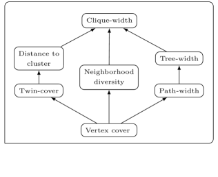
Figure 1:  A schematic showing the relation between various parameters. There is an arrow from parameter $k_{1}$ to $k_{2}$, if there exists a function $f$ such that for all graphs $G$, we have $k_{2}(G)\leq f(k_{1}(G))$.

In the direction of restricted classes of graphs, there has been many results on planar graphs, the latest of which is by Huang, Guo, and Yuan [19], who showed that four colors are sufficient to CFON* color planar graphs. Given the motivation from the frequency assignment problem, it is natural to consider the intersection graphs. Several intersection graphs have been considered, such as string graphs and circle graphs [20]. Fekete and Keldenich [12] studied CFCN^∗ coloring on common intersection graphs such as interval graphs, unit disk graphs and unit square graphs. (See the reference therein for further related works on intersection graphs.) Reddy [29] showed that interval graphs can be CFON^∗ colored by at most four colors. It was an open question from [12, 29] that whether the 4-color bound can be improved (or is tight) and does there exist a polynomial time algorithm for the CFON^∗ problem on interval graphs. Recently, the latter problem was proved affirmatively by Gonzalez and Mann [17].

Moreover, continuing the line of investigation, we study these problems on other restricted graph classes such as distance-hereditary graphs, Kneser graphs and split graphs. Similar for other graph classes that were studied before, we consider the two main questions on the the worst-case bounds on the required number of colors and the computational complexity to decide whether $k$ colors are sufficient to conflict-free color these classes of graphs.

1.1 Results and Discussion

We now discuss the results of the paper. A summary of the results for CFON* and CFCN* colorings, are presented in Tables 1 and 2 respectively.

• In Section 3, we show FPT algorithms for both CFON* and CFCN* problems with respect to the combined parameters clique width $w$ and the solution size $k$, that runs in $2^{O(w3^{k})}n^{O(1)}$ time, where $n$ is the number of vertices.

  We show that unlike some other parameters, the conflict-free chromatic numbers are not bounded by a function of clique width. Towards this, we show the existence of graphs $G$ such that $cw(G)=3$ and $\chi_{CN}^{*}(G)=O(\log n)$. We show a similar bound for the CFON* chromatic number. This rules out the possibility that our algorithms are FPT when parameterized by clique width alone. However, one could show the FPT result through a different approach.

• In Section 4, we discuss certain graphs with bounded clique width. In particular, for distance-hereditary graphs $G$, we show that $\chi^{*}_{CN}(G){}\leq 3$. Hence, our CFCN^∗ coloring FPT algorithm in Section 3 implies a polynomial time algorithm for this class of graphs. Their CFON* chromatic number, however, is unbounded. However, we show that it is bounded for two subclasses, cographs and block graphs, and hence the CFON* problem is polynomial time solvable on them.

• In Section 5, we show that for interval graphs $G$, $\chi^{*}_{ON}(G){}\leq 3$, and that this bound is tight. Moreover, two colors are sufficient to CFON* color proper interval graphs. We also show that the CFCN* problem is polynomial time solvable on interval graphs.

• In Section 6, we consider the unit square and unit disk intersection graphs. We show that $\chi^{*}_{ON}(G){}\leq 27$ for unit square graphs $G$. For unit disk graphs $G$, we show that $\chi^{*}_{ON}(G){}\leq 54$. No upper bound was known previously.

  In Section 7, we show that the CFON* problem is NP-complete on unit disk intersection graphs and unit square intersection graphs.

• In Section 8, we study both problems on Kneser graphs $K(n,k)$. We show that $k+1$ colors are sufficient when $n\geq 2k+1$ and are also necessary when $n\geq 2k^{2}+k$. For CFCN* coloring of $K(n,k)$, we prove an upper bound of $k$ colors for $n\geq 2k+1$.

• In Section 9, we study both problems on split graphs. We show that the CFON* problem is NP-complete and the CFCN* problem is polynomial time solvable.

Graph Class	Upper Bound	Lower Bound	Complexity
$(G,{\sf cw},k)$	-	-	FPT
Distance hereditary graphs	-	$\Omega(\log n)$	-
Block graphs	3	3 (Fig. 5)	P
Cographs	2	2 ($K_{3}$)	P
Interval graphs	3	3 (Fig. 6)	P [17]
Proper interval graphs	2	2 ($K_{3}$)	P [17]
Unit square graphs	27	3 (Fig. 7)	NP-hard
Unit disk graphs	54	3 (Fig. 7)	NP-hard
Kneser graphs $K(n,k)$	$k+1$	$k+1$	-
Split graphs	-	-	NP-hard

Table 1: Bounds and algorithmic status on various graph classes for the CFON* problem. Here a “Lower Bound” of $\ell$ indicates existence of a graph $G$ such that $\chi^{*}_{ON}(G){}=\ell$. If the algorithmic status (whether P or NP-hard) for a graph class is unknown, we indicate it by “-”. The graphs for lower bounds are indicated in parentheses. $K_{3}$ refers to the complete graph on 3 vertices. The lower bound proof for distance hereditary graphs is shown in Lemma 3. The lower bound for Kneser graphs only applies for $n\geq 2k^{2}+k$; see Lemma 14.

Graph Class	Upper Bound	Lower Bound	Complexity
$(G,{\sf cw},k)$	-	-	FPT
Distance Hereditary Graphs	3	2 (Fig. 3)	P
Block graphs	2	2 (Fig 3)	P
Cographs	2	2 ($K_{2,2}$)	P
Interval graphs	2[12]	2 (Fig. 3)	P
Proper interval graphs	2[12]	2 (Fig. 3)	P
Unit square graphs	4[12]	2 (Fig. 3)	NP-hard [12]
Unit disk graphs	6[12]	2 (Fig. 3)	NP-hard [12]
Kneser graphs $K(n,k)$	$k$	-	-
Split graphs	2	2 (Fig. 3)	P

Table 2: Bounds and algorithmic status on various graph classes for the CFCN* problem. Here a “Lower Bound” of $\ell$ indicates existence of a graph $G$ such that $\chi^{*}_{CN}(G){}=\ell$. If the algorithmic status (whether P or NP-hard) for a graph class is unknown, we indicate it by “-”. For all graph classes except cographs, the bull graph in Figure 3 is the graph that requires 2 colors. For cographs, the complete bipartite graph $K_{2,2}$ is the graph that requires 2 colors.

2 Preliminaries

Throughout the paper, we assume that the graph $G$ is connected. Otherwise, we apply the algorithm on each component independently. We also assume that $G$ does not contain any isolated vertices as the CFON* problem is not defined for an isolated vertex. We use $[k]$ to denote the set $\{1,2,\dots,k\}$ and $C:V(G)\rightarrow\{0\}\cup[k]$ to denote the color assigned to a vertex. A universal vertex is a vertex that is adjacent to all other vertices of the graph. In some of our algorithms and proofs, it is convenient to distinguish between vertices that are intentionally left uncolored, and the vertices that are yet to be assigned any color. The assignment of color 0 is used to denote that a vertex is left “uncolored”.

To avoid clutter and to simplify notation, we use the shorthand notation $vw$ to denote the edge $\{v,w\}$. The open neighborhood of a vertex $v\in V(G)$ is the set of vertices $\{w:vw\in E(G)\}$ and is denoted by $N(v)$. Given a conflict-free coloring $C$, a vertex $w\in N(v)$ is called a uniquely colored neighbor of $v$ if $C(w)\neq 0$ and $\forall x\in N(v)\setminus\{w\},C(w)\neq C(x)$. The closed neighborhood of $v$ is the set $N(v)\cup\{v\}$, denoted by $N[v]$. The notion of a uniquely colored neighbor in the closed neighborhood variant is analogous to the open neighborhood variant, and is obtained by replacing $N(v)$ by $N[v]$. We sometimes use the mapping $h:V\rightarrow V$ to denote the uniquely colored neighbor of a vertex. We also extend $C$ for vertex sets by defining $C(V^{\prime})=\bigcup_{v\in V^{\prime}}C(v)$ for $V^{\prime}\subseteq V(G)$. To refer to the multi-set of colors used in $V^{\prime}$, we use $C_{\{\!\!\{\}\!\!\}}(V^{\prime})$. The difference between $C_{\{\!\!\{\}\!\!\}}(V^{\prime})$ and $C(V^{\prime})$ is that we use multiset union in the former.

A parameterized problem is denoted as $(I,k)\subseteq\Sigma^{*}\times\mathbb{N}$, where $\Sigma$ is fixed alphabet and $k$ is called the parameter. We say that the problem $(I,k)$ is fixed-parameter tractable (FPT in short) with respect to the parameter $k$ if there exists an algorithm which solves the problem in time $f(k)|I|^{O(1)}$, where $f$ is a computable function. For more details on parameterized complexity, we refer the reader to the texts [8, 10].

In many of the sections, we also refer to the full coloring variant of the conflict-free coloring problem, defined as follows.

Definition 2 (Conflict-Free Coloring – Full Coloring Variant)

A CFON coloring of a graph $G=(V,E)$ using $k$ colors is an assignment $C:V\rightarrow\{1,2,\ldots,k\}$ such that for every $v\in V$, there exists an $i\in\{1,2,\ldots,k\}$ such that $|N(v)\cap C^{-1}(i)|=1$. The smallest number of colors required for a CFON coloring of $G$ is called the CFON chromatic number of $G$, denoted by $\chi_{ON}(G){}$.

The corresponding closed neighborhood variant is denoted CFCN coloring, and the chromatic number is denoted $\chi_{CN}(G)$.

A full conflict-free coloring, where all the vertices are colored with a non-zero color, is also a partial conflict-free coloring (as defined in Definition 1) while the converse is not true. It is clear that one extra color suffices to obtain a full coloring variant from a partial coloring variant. However, it is not always clear if the extra color is actually necessary.

Related to the conflict-free coloring problem is the classical NP-complete graph coloring problem. In this problem, given a graph $G$, we would like to minimize the number of colors required to color every vertex in $G$ such that adjacent vertices have different colors. The solution to this problem is called the chromatic number of $G$, denoted by $\chi(G)$. Observe that such a coloring gives a CFCN coloring, but in general, the CFCN chromatic number is much lower than the chromatic number. For example, $\chi(K_{n})=n$ but $\chi_{CN}(K_{n})=2$ where $K_{n}$ is a clique on $n$ vertices.

3 FPT with Clique Width and Number of Colors

In this section, we study the conflict-free coloring problem with respect to the combined parameters clique width $cw(G)$ and number of colors $k$. We present FPT algorithms for both the CFON* and CFCN* problems.

Definition 3 (Clique width [7])

Let $w\in\mathbb{N}$. A $w$-expression $\Phi$ defines a graph $G_{\Phi}$ where each vertex receives a label from $[w]$, using the following four recursive operations with indices $i,j\in[w]$, $i\neq j$:

1. Introduce, $\Phi=v(i)$: $G_{\Phi}$ is a graph consisting a single vertex $v$ with label $i$.

2. Disjoint union, $\Phi=\Phi^{\prime}\oplus\Phi^{\prime\prime}$: $G_{\Phi}$ is a disjoint union of $G_{\Phi^{\prime}}$ and $G_{\Phi^{\prime\prime}}$.

3. Relabel, $\Phi=\rho_{i\rightarrow j}(\Phi^{\prime})$: $G_{\Phi}$ is the graph $G_{\Phi^{\prime}}$ where each vertex labeled $i$ in $G_{\Phi^{\prime}}$ now has label $j$.

4. Join, $\Phi=\eta_{i,j}(\Phi^{\prime})$: $G_{\Phi}$ is the graph $G_{\Phi^{\prime}}$ with additional edges between each pair of vertices $u$ of label $i$ and $v$ of label $j$.

The clique width of a graph $G$ denoted by cw(G) is the minimum number $w$ such that there is a $w$-expression $\Phi$ that defines $G$.

In the following, we assume that a $w$-expression $\Psi$ of $G$ is given. There is an FPT-algorithm that, given a graph $G$ and integer $w$, either reports that $\operatorname{cw}(G)>w$ or outputs a $(2^{3w+2}-1)$-expression of $G$ [26]. Further, we can assume WLOG that a $w$-expression uses at most $n$ disjoint unions and $O(nw^{2})$ other operations [7].

A $w$-expression $\Psi$ is an irredundant $w$-expression of $G$, if no edge is introduced twice in $\Psi$. Given a $w$-expression of $G$, it is possible to get an irredundant $w$-expression of $G$ in polynomial time [7]. For a coloring of $G$, a vertex $v$ is said to be conflict-free dominated by the color $c$, if exactly one vertex in $N(v)$ is assigned the color $c$. In general, a vertex $v$ is said to be conflict-free dominated by a set of colors $S$, if each color in $S$ conflict-free dominates $v$. Also, a vertex $v$ is said to miss the color $c$ if there exists no vertex in $N(v)$ that is assigned the color $c$. In general, a vertex $v$ is said to miss a set of colors $T$, if every color in $T$ is missed by $v$.

Now, we prove the main theorem of this section.

Theorem 3.1

Given a graph $G$, a $w$-expression of $G$ and an integer $k$, it is possible to decide if $\chi^{*}_{ON}(G){}\leq k$ in $2^{O(w3^{k})}n^{O(1)}$ time.

Proof

We give a dynamic program that works bottom-up over a given irredundant $w$-expression $\Psi$ of $G$. For each subexpression $\Phi$ of $\Psi$, we have a boolean table entry $d[\Phi;N;M]$ with

$$N=(n_{1,0},\ldots,n_{1,k},\ldots,n_{w,0},\ldots,n_{w,k})\in\{0,1,2\}^{w(k+1)},\mbox{ and}$$

$$M=(M_{1},\dots,M_{w})\quad\text{where for }a\in[w],M_{a}=(m_{a,S_{1},T_{1}},\dots,m_{a,S_{3^{k}},T_{3^{k}}})\in\{0,1\}^{3^{k}}$$

where $S_{\ell},T_{\ell}$ are all the possible pairs of disjoint subsets of the set of colors $[k]$. Note that there are $3^{k}$ many pairs of disjoint subsets $S_{\ell},T_{\ell}\in[k]$.

The boolean entry $d[\Phi;N;M]$ is then set to TRUE if and only if there exists a vertex-coloring $C:V(G_{\Phi})\to\{0\}\cup[k]$ such that:

• For each label $a\in[w]$ and color $q\in\{0\}\cup[k]$, the variable $n_{a,q}$ in $N$ is the number of vertices of $G_{\Phi}$ with label $a$ that are colored $q$, capped at two. In other words, if ${n}_{a,q}^{\star}$ be the number of vertices with label $a$ that are colored $q$, then ${n}_{a,q}=\min\{2,n_{a,q}^{\star}\}$.

• For each label $a\in[w]$ and disjoint sets $S,T\subseteq[k]$, the variable $m_{a,S,T}$ in $M$ has value 1, if and only if there exists a vertex $v$ with label $a$, such that $v$ is conflict-free dominated by exactly the colors in $S$ and the set of colors that misses $v$ is exactly $T$.

Intuitively, for this coloring, $N$ describes the number of occurrences of a color among the vertices of a particular label. Moreover, $M$ gives a “profile” of vertices in the graph by their labels and the sets of colors that they are conflict-free dominated and are missed.

To decide if $k$ colors are sufficient to CFON* color $G$, we consider the expression $\Psi$ with $G_{\Psi}=G$. We answer ‘yes’ if and only if there exists an entry $d[\Psi;N;M]$ set to TRUE where $m_{a,\emptyset,T}=0$ for each $a\in[w]$ and for each $T\subseteq[k]$. This means there exists a coloring such that there is no label $a\in[w]$ with a vertex $v$ that is not conflict-free dominated.

Now, we show how to compute $d[\Phi;N;M]$ at each operation.

1. $\Phi=v(i)$.

   The graph $G_{\Phi}$ represents a node with one vertex $v$ that is labeled $i\in[w]$. For each color $q\in\{0\}\cup[k]$, we set the entry $d[\Phi;N;M]=\mbox{TRUE}$ if and only if $n_{i,q}=1$, $m_{i,\emptyset,[k]}=1$ and all other entries of $N$ and $M$ are $0$.

2. $\Phi=\Phi^{\prime}\oplus\Phi^{\prime\prime}$.

   The graph $G_{\Phi}$ results from the disjoint union of graphs $G_{\Phi^{\prime}}$ and $G_{\Phi^{\prime\prime}}$.

   We set $d[\Phi;N;M]=\mbox{TRUE}$ if and only if there exist entries $d[\Phi^{\prime};N^{\prime};M^{\prime}]$ and $d[\Phi^{\prime\prime};N^{\prime\prime};M^{\prime\prime}]$ such that $d[\Phi^{\prime};N^{\prime};M^{\prime}]=\mbox{TRUE}$, $d[\Phi^{\prime\prime};N^{\prime\prime};M^{\prime\prime}]=\mbox{TRUE}$ and the following conditions are satisfied:

   1. For each label $a\in[w]$ and color $q\in\{0\}\cup[k]$, $n_{a,q}=\min\{2,\;n^{\prime}_{a,q}+n^{\prime\prime}_{a,q}\}$.

   2. For each label $a\in[w]$ and disjoint $S,T\subseteq[k]$, $m_{a,S,T}=\min\{1,\;m^{\prime}_{a,S,T}+m^{\prime\prime}_{a,S,T}\}$.

   We may determine each table entry of $d[\Phi;N,M]$ for every $N,M$ as follows. We initially set $d[\Phi;N,M]$ to FALSE for all $N,M$. We iterate over all combinations of table entries $d[\Phi^{\prime};N^{\prime};M^{\prime}]$ and $d[\Phi^{\prime\prime};N^{\prime\prime};M^{\prime\prime}]$. For each combination of TRUE entries $d[\Phi^{\prime};N^{\prime};M^{\prime}]$ and $d[\Phi^{\prime\prime};N^{\prime\prime};M^{\prime\prime}]$, we update the corresponding entry $d[\Phi;N;M]$ to TRUE. This corresponding entry $d[\Phi;N;M]$ has variables $n_{a,q}$ which is the sum of $n_{a,q}^{\prime}$ and $n_{a,q}^{\prime\prime}$ limited by two, and variables $m_{a,S,T}$ which is the sum of $m_{a,S,T}^{\prime}$ and $m_{a,S,T}^{\prime\prime}$ limited by one. Thus, to compute every entry for $d[\Phi;;]$ we visit at most $(3^{w(k+1)}2^{w3^{k}})^{2}$ combinations of table entries and for each of those compute $w(k+1)+w3^{k}$ values for $N$ and $M$.

3. $\Phi=\rho_{i\rightarrow j}(\Phi^{\prime})$.

   The graph $G_{\Phi}$ is obtained from the graph $G_{\Phi^{\prime}}$ by relabeling the vertices of label $i$ in $G_{\Phi^{\prime}}$ with label $j$ where $i,j\in[w]$. Hence, $n_{i,q}=0$ for each $q\in\{0\}\cup[k]$ and $m_{i,S,T}=0$ for each disjoint $S,T\subseteq[k]$.

   We set $d[\Phi;N;M]=\mbox{TRUE}$ if and only if there exists an entry $d[\Phi^{\prime};N^{\prime};M^{\prime}]$ such that $d[\Phi^{\prime};N^{\prime};M^{\prime}]=\mbox{TRUE}$ in $G_{\Phi^{\prime}}$ and satisfies the following conditions:

   1. For each color $q\in\{0\}\cup[k]$, each label $a\in[w]\setminus\{i,j\}$ and disjoint $S,T\subseteq[k]$, $n_{a,q}=n^{\prime}_{a,q}$ and $m_{a,S,T}=m^{\prime}_{a,S,T}$.

   2. For each color $q\in\{0\}\cup[k]$, $n_{j,q}=\min\{2,\;n^{\prime}_{i,q}+n^{\prime}_{j,q}\}$ and $n_{i,q}=0$.

   3. For each disjoint $S,T\subseteq[k]$, $m_{j,S,T}=\min\{1,\;m^{\prime}_{i,S,T}+m^{\prime}_{j,S,T}\}$ and $m_{i,S,T}=0$.

   We may determine each table entry of $d[\Phi;N;M]$ for every $N,M$ as follows. We initially set $d[\Phi;N;M]$ to FALSE for all $N,M$. We iterate over all the TRUE table entries $d[\Phi^{\prime};N^{\prime};M^{\prime}]$, and for each such entry we update the corresponding entry $d[\Phi;N;M]$ to TRUE, if applicable. To compute every entry for $d[\Phi;;]$ we visit at most $3^{w(k+1)}2^{w3^{k}}$ table entries $d[\Phi^{\prime};;]$ and for each of those compute $w(k+1)+w3^{k}$ values for $M$ and $N$.

4. $\Phi=\eta_{i,j}(\Phi^{\prime})$.

   The graph $G_{\Phi}$ is obtained from the graph $G_{\Phi^{\prime}}$ by connecting each vertex with label $i$ with each vertex with label $j$ where $i,j\in[w]$. Consider a vertex $v$ labeled $i$ in $G_{\Phi^{\prime}}$. Suppose $v$ contributes to the variable $m^{\prime}_{i,\widehat{S},\widehat{T}}$, i.e., $v$ is conflict-free dominated by exactly $\widehat{S}$ and the set of colors that misses $v$ is exactly $\widehat{T}$. After this operation, the vertex $v$ may contribute to the variable $m_{i,S,T}$ in $G_{\Phi}$ where the choice of the sets $S$ and $T$ in $G_{\Phi}$ depends on the colors assigned to the vertices labeled $j$ in $G_{\Phi^{\prime}}$.

   More specifically, we set $d[\Phi;N;M]=\mbox{TRUE}$ if and only if there exists an entry $d[\Phi^{\prime};N^{\prime};M^{\prime}]$ such that $d[\Phi^{\prime};N^{\prime};M^{\prime}]=\mbox{TRUE}$ in $G_{\Phi^{\prime}}$ and satisfies the following conditions:

   1. For each label $a\in[w]$ and color $q\in\{0\}\cup[k]$, $n_{a,q}=n^{\prime}_{a,q}$.

   2. For each label $a\in[w]\setminus\{i,j\}$ and disjoint $S,T\subseteq[k]$, $m_{a,S,T}=m^{\prime}_{a,S,T}$.

   3. For the label $i$ and disjoint $S,T\subseteq[k]$, $m_{i,S,T}=1$ if and only if there are disjoint subsets $\widehat{S},\widehat{T}\subseteq[k]$ with $m^{\prime}_{i,\widehat{S},\widehat{T}}=1$ such that

      1. For each color $q\in S\cap\widehat{S}$, variable $n^{\prime}_{j,q}=0$.

      2. For each color $q\in S\setminus\widehat{S}$, variable $n^{\prime}_{j,q}=1$.

      3. For each color $q\in\widehat{S}\setminus S$, variable $n^{\prime}_{j,q}\geq 1$.

      4. $S\setminus\widehat{S}\subseteq\widehat{T}$ and $T\subseteq\widehat{T}$.

      5. For each color $q\in\widehat{T}\setminus(T\cup S)$, $n^{\prime}_{j,q}=2$.

   4. For the label $j$, entry $m_{j,S,T}$ is computed in a symmetric fashion by swapping the labels $i$ and $j$ in (c).

   It can be observed that each TRUE table entry $d[\Phi^{\prime};N^{\prime};M^{\prime}]$ sets exactly one entry $d[\Phi;N;M]$ to TRUE. We can determine each table entry of $d[\Phi;N;M]$ as follows. We initially set $d[\Phi;N,M]$ to FALSE for all $N,M$. We iterate over all the TRUE table entries $d[\Phi^{\prime};N^{\prime};M^{\prime}]$, and for each such entry we update the corresponding entry $d[\Phi;N;M]$ to TRUE, if applicable. To compute every entry for $d[\Phi;;]$ we visit at most $3^{w(k+1)}2^{w3^{k}}$ table entries $d[\Phi^{\prime};;]$ and for each of those compute $w(k+1)+w3^{k}$ values for $M$ and $N$.

We described the recursive formula at each operation, that computes the value of each entry $d[;;]$. The correctness of the algorithm easily follows from the description of the algorithm. The DP table consists of $3^{w(k+1)}2^{w3^{k}}$ entries at each node of the $w$-expression. Since we assume that there are at most $n$ disjoint unions and $nw^{2}$ other operations, it is easy to see that the running time is dominated by the operations at all the disjoint unions that requires in total $O(3^{2w(k+1)}2^{2w3^{k}}w(k+1+3^{k})n)$ time. The time bound then follows. ∎

Similarly, we obtain the following result for the CFCN* problem:

Theorem 3.2

Given a graph $G$, a $w$-expression and an integer $k$, it is possible to decide if $\chi^{*}_{CN}(G){}\leq k$ in $2^{O(w3^{k})}n^{O(1)}$ time.

Proof

The computation of the entries $d[;;]$ at the disjoint union node, relabel node and join node is the same as discussed in Theorem 3.1. However, we replace the open neighborhood $N(v)$ with the closed neighborhood $N[v]$ in the definitions of conflict-free domination by a color $c$ and missing a color $c$. Now we discuss the computation of the entry $d[;;]$ at the introduce node.

Introduce Node $\Phi=v(i)$: The graph $G_{\Phi}$ represents a node with one vertex $v$ that is labeled $i$. For each color $q\in[k]$, we set the entry $d[\Phi;N;M]=$ TRUE if each variable is 0 except $n_{i,q}=1$ and $m_{i,\{q\},[k]\setminus\{q\}}=1$.

For the case when $q=0$, we set the entry $d[\Phi;N;M]=\mbox{TRUE}$ if each variable is 0 except $n_{i,0}=1$ and $m_{i,\emptyset,[k]}=1$. ∎

By modifying the above algorithm, it is possible to obtain FPT algorithms for the full coloring variants (CFON and CFCN) of the problem. We merely have to restrict the entries of the dynamic program to entries without color 0.

Theorem 3.3

The CFON and the CFCN problems are FPT when parameterized by the combined parameters clique width and the solution size.

3.1 Graphs of bounded clique width and unbounded $\chi_{CN}$ and $\chi_{ON}$

An open question is then whether there exists an FPT algorithm with respect to only the clique width. One approach to this question is to bound the CFON and the CFCN chromatic numbers by a function of the clique width. However, this turns out to be false, even for graphs of clique width three. Specifically, we inductively construct graphs $G_{2},G_{3},\dots,G_{k}$ such that $G_{i}$ requires at least $i$ colors, but has clique width at most $3$. This bound is tight, since graphs of clique width at most $2$, i.e. co-graphs, have bounded CFON and the CFCN numbers, as shown in Theorems 2 and 4 in the next section. In the following, we consider the full coloring variant. Let us first consider a CFCN-coloring.

Theorem 3.4

For any given integer $k$ $\geq 2$, there exists a graph $G_{k}$ of clique width at most 3 with $\chi_{CN}(G_{k})\geq k$.

Figure 2: $G_{3}$ (left) and $G_{4}$ (right) have clique-width $3$ but cannot be CFCN-colored with $2$ and $3$ colors, respectively. Each $G_{i}$,$i\geq 2$ stands for a copy of the graph $G_{i}$. Every vertex in an ellipse is adjacent to every vertex that is connected to that ellipse.

Proof

We construct graphs $G_{i}$, $i\geq 2$ inductively. Graph $G_{k+1}$ is such that it cannot be CFCN-colored with $k$ colors. Thus at least $k+1$ colors are required.

• Let $G_{2}$ be the graph consisting of a single edge.

• Let $G_{k+1}$, for $k\geq 2$, consist of $2^{k}$ bottom vertices $B=\{b_{0},\dots,b_{2^{k}-1}\}$, which form a clique. Let $T$ be the full binary tree with $k$ levels and with leaves $B$: That is, $T$ consists of $k+1$ levels $L_{0},\dots,L_{k}$, where level $L_{i}$ contains $2^{k-i}$ vertices $b_{0}^{i},\dots,b_{2^{k-i}-1}^{i}$ for $0\leq i\leq k$. Each vertex $b_{j}^{i}$ has children $b_{2j}^{i-1}$ and $b_{2j+1}^{i-1}$ for $1\leq i\leq k$ and $0\leq j<2^{k-i}$. Then we identify the bottom vertices $B$ with the leaves $L_{0}$, which is $b^{0}_{j}=b_{j}$ for $0\leq j<2^{k}$. For a non-leaf $x$ of $T$, let $B(x)\subseteq B$ be the set of descendants of $x$ among the leaves $B$. Let $\mathcal{B}=\{B(x)\mid x\in V(T)\setminus L_{0}\}$ be the family of such sets. For every set $S\in\mathcal{B}$, introduce two disjoint copies of $G_{k}$ and make them adjacent to $S$, i.e., all the vertices in the two copies of $G_{k}$ are adjacent to all the vertices in $S$. See Fig 2 for illustrations.

Inductively we show that $G_{k}$ has clique width at most $3$. That is, there is a $3$-expression $\Phi_{k}$ where $G_{\varphi_{k}}$ equals $G$ when ignoring the labels. Let us use the labels $\{\alpha,\beta,\gamma\}$ instead of numbers, since numbers are already used for colors.

• Graph $G_{2}$, a single edge, can be constructed using 2 labels.

• Consider graph $G_{k+1}$. By the induction hypothesis, there is a $3$-expression $\Phi_{k}$ that describes $G_{k}$. We may assume that every vertex of $G_{\Phi_{k}}$ has label $\beta$ since we can add final re-label operations. Let vertex sets $B$ and $T$ with levels $L_{0},\dots,L_{k}$ be as in the construction of $G_{k+1}$. We show the following properties for every node $x\in L_{i}$ of $T$ by induction on the level $i=0,\dots,k$:

  • There is a 3-expression $\Phi_{k+1,x}$ where $G_{\Phi_{k+1,x}}$ equals the induced subgraph of $G_{k+1}$ that contains $B(x)$ and the copies of $G_{k}$ with neighborhood $B(x)$; and

  • $B(x)$ has label $\alpha$ and the copies of $G_{k}$ have label $\gamma$.

  Then $\Phi_{k+1,r}$, where $r$ is the root of $T$, is the desired $3$-expression.

  • For the induction basis, $i=0$ and $x\in L_{0}$, hence $x$ is some leaf $b_{i}$: Simply introduce the single vertex of label $\alpha$.

  • For the induction step, $i\geq 1$ and $x\in L_{i}$. Then $x$ has some children $y$ and $z$ in level $L_{i-1}$. Thus by induction hypothesis there are $3$-expressions $\Phi_{k+1,y}$ and $\Phi_{k+1,z}$ with the properties described above. We construct $\Phi_{k,x}$: Join $\Phi_{k+1,y}$ and $\Phi_{k+1,z}$ and add all edges between $B(y)$ and $B(z)$. To do so we actually join $\rho_{\alpha\to\beta}(\Phi_{k+1,y})$ and $\Phi_{k+1,z}$, add all edges between $\alpha$ and $\beta$, and then re-label $\beta$ to $\alpha$ again. Introduce two copies of $G_{k}$ by joining twice with $\Phi_{k}$ (that has label $\beta$ only). Then add all edges between $B(x)=B(y)\cup B(z)$ (of label $\alpha$) and the new copies of $G_{k}$ (of label $\beta$).

    Now we have introduced all vertices of the restricted version of $G_{k+1}$ as described above. It remains to satisfy the labeling. Thus, as the last step, re-label $\beta$ to $\gamma$.

Lastly, we show by induction that $G_{k+1}$ has no $CFCN{}$-coloring with only $k$ colors, for every $k\geq 1$. For the induction basis, consider $G_{2}$, a single edge. There, a $1$-coloring is not possible.

For the induction step, $G_{k}\leadsto G_{k+1}$, assume for the sake of contradiction, that there is a CFCN-coloring $c:V(G_{k+1})\to\{1,\dots,k\}$.

We first show that each set $S\in\mathcal{B}$ contains a uniquely colored vertex $f(S)$. Formally, there is a mapping $f:\mathcal{B}\to B$ such that for each set $S\in\mathcal{B}$ there is a vertex $f(S)=v\in S$ such that $c(v)\neq c(v^{\prime})$ for every other vertex $v^{\prime}\in S\setminus\{v\}$. Recall that $G_{k+1}$ contains two copies $C_{1},C_{2}$ of $G_{k}$ where each $C_{i},i\in\{1,2\}$ has $N(C_{i})\setminus C_{i}=S$. Now assume, for the sake of contradiction, that $S$ contains no uniquely colored vertex. Let $c_{i}$ be the coloring $c$ restricted to vertices $V(C_{i})$, for $i\in\{1,2\}$. Then $c_{i}$ is a CFCN-coloring of graph $C_{i}$, for $i\in\{1,2\}$. By induction hypothesis, the restricted coloring $c_{i}$ maps to all $k$ colors. Hence in $V(C_{1})\cup V(C_{2})$ every of the $k$ colors occurs twice. However, then every vertex in $u\in S$ has every color $\{1,\dots,k\}$ at least twice in its neighborhood. A contradiction to that $u$ have a uniquely colored neighbor. Therefore, each set $S\in\mathcal{B}$ contains a uniquely colored vertex $f(S)$.

Now, by symmetry we may assume that the uniquely colored element of set $B$ is $f(B)=b_{2^{k}-1}$ and $b_{2^{k}-1}$ is colored with color $k$. Then the subset $\{b_{0},\dots,b_{2^{k-1}-1}\}\in\mathcal{B}$ may only consists of vertices of color $1,\dots,k-1$. Again by symmetry, we may assume that this subset $\{b_{0},\dots,b_{2^{k-1}-1}\}$ has uniquely colored element $f(\{b_{0},\dots,b_{2^{k-1}-1})\}=b_{2^{k-1}-1}$ and vertex $b_{2^{k-1}-1}$ is colored with ${k-1}$. By repeating this argument, we eventually obtain that $f(\{b_{1},b_{2}\})$ must be colors with color $1$ only. A contradiction to that $\{b_{1},b_{2}\}\in\mathcal{B}$ has a uniquely colored element. Therefore, $G_{k+1}$ cannot be colored with just $k$ colors. ∎

To show that the CFON coloring number is also unbounded even for graphs with clique width three, we can define a sequence of graphs $G_{2}^{\prime},G_{3}^{\prime},\dots$ analogously as we did for CFCN coloring. That is, each graph $G_{k+1}^{\prime}$ for $k\geq 2$ has clique width at most three and cannot be CFCN colored with only $k$ colors. Let $G_{2}^{\prime}$ be a triangle, which cannot be CFON-colored with only one color and which has clique width at most $3$. We construct $G_{k+1}^{\prime}$ using copies of $G_{k}^{\prime}$ in the same way as we constructed $G_{k+1}$ using copies of $G_{k}$. Again, inductively it follows that $G_{k+1}^{\prime}$ has clique width at most $3$. Also, by the same induction step as before, it follows that $G_{k+1}^{\prime}$ cannot be CFON colored with only $k$ colors. We also provide an alternative construction in Lemma 3.

Theorem 3.5

For any given integer $k$ $\geq 2$, there exists a graph $G_{k}$ of clique width at most 3 with $\chi_{ON}(G_{k})\geq k$.

4 Classes of Graphs with Bounded Clique Width

One consequence of Theorem 3.1 (or Theorem 3.2) is that if both clique width and the CFON* (or CFCN*, respectively) chromatic numbers are bounded, then there exists a polynomial algorithm to solve the CFON* (or CFCN*, respectively) problem. Theorems 3.4 and 3.5 show that even when the clique width is at most 3, the CFON* and CFCN* chromatic numbers can be unbounded. However, in this section, we discuss some classes of graphs with clique width at most 3, where the CFON* or CFCN* chromatic number is bounded.

Firstly, if we consider the graphs with clique width at most 2, these are exactly cographs [7].

Definition 4 (Cograph [6])

A graph $G$ is a cograph if $G$ consists of a single vertex, or if it can be constructed from a single vertex graph using the disjoint union and complement operations.

We will show that the cographs have CFCN* and CFON* chromatic numbers at most 2 (Lemmas 2 and 4).

These graphs are a special case of distance hereditary graphs, whose clique width is at most 3 [16].

Definition 5 (Distance hereditary graph [18])

A graph $G$ is distance hereditary if for every connected induced subgraph $H$ of $G$, the distance (i.e., the length of a shortest path) between any pair of vertices in $H$ is the same as that in $G$.

Bandelt and Mulder [3] showed that for any connected distance hereditary graph $G$, there exists a one-vertex extension sequence $(v_{1},v_{2},\dots,v_{n})$, defined as follows. Denote by $G[i]$ the induced subgraph of $G$ on $\{v_{1},\dots,v_{i}\}$. The sequence $(v_{1},v_{2},\dots,v_{n})$ is a one-vertex extension sequence if $G[2]=K_{2}$, and for any $i\geq 3$, $G[i]$ can be formed by adding $v_{i}$ to $G[i-1]$ and adding edges such that for some $j<i$, one of the following holds:

• $v_{i}$ is only adjacent to $v_{j}$ (we call $v_{i}$ is a pendant of $v_{j}$);

• $v_{i}$ is adjacent to all the neighbors of $v_{j}$ (we call $v_{i}$ is a false twin of $v_{j}$); or

• $v_{i}$ is adjacent to $v_{j}$ and all the neighbors of $v_{j}$ (we call $v_{i}$ is a true twin of $v_{j}$).

Note that if the pendant operation is absent, then we have exactly cographs. In other words, cographs are exactly the distance hereditary graphs that can be constructed from a single vertex by the true twin and false twin operations [3]. If the true twin operation is absent, then we obtain bipartite distance hereditary graphs. Lastly, if the false twin operation is missing, we obtain a subclass of graphs that contain block graphs [24].

Definition 6 (Block Graph)

A block graph is a graph in which every 2-connected component (i.e., a maximal subgraph which cannot be disconnected by the deletion of one vertex) is a clique.

It turns out that the distance hereditary graphs in general have a bounded CFCN* chromatic number but an unbounded CFON* chromatic number. However, for the subclasses of cographs and block graphs, the CFON* chromatic number is bounded.

4.1 CFCN* chromatic number

In this section, we discuss the CFCN* chromatic number of distance hereditary graphs and some subclasses.

Lemma 1

If $G$ is a distance hereditary graph $G$, then $\chi^{*}_{CN}(G)\leq 3$.

Proof

Suppose $(v_{1},v_{2},\dots,v_{n})$ is a one-vertex extension sequence of $G$. We will devise an iterative algorithm to provide a CFCN* coloring with colors 0, 1, 2, 3.

We use $N_{i}(v)$ and $N_{i}[v]$ to respectively refer to the open and closed neighborhoods of a vertex $v$ in the graph $G[i]$, where $i\in[n]$ is the current iteration of the algorithm.

For each vertex $v$, we will specify a tuple $\mathcal{C}(v)=(a,b)$, where $a\in\{0,1,2,3\}$ is the color of $v$, and $b\in\{1,2,3\}$ will be shown later to correspond to the color of the uniquely colored neighbor of $v$. In fact, we will maintain the following two invariants at the end of every iteration $i\in[n]$ of the coloring algorithm:

• Invariant 1: For all $v\in G[i]$, if $\mathcal{C}(v)=(a,b)$, then $b$ is the color of the uniquely colored neighbor of $v$ in $G[i]$.

• Invariant 2: For all $v\in G[i]$, if $\mathcal{C}(v)=(a,a)$, then either (*) all vertices $w$ in $N_{i}(v)$ satisfy $\mathcal{C}(w)=(0,d)$ where $d$ is a fixed color with $d\neq a$, or (**) there is a vertex with a unique (nonzero) color among the vertices in $N_{i}(v)$.

We are now ready to describe the coloring scheme. Recall that $v_{1}$ and $v_{2}$ are adjacent to one another. We assign $\mathcal{C}(v_{1})=(1,2)$ and $\mathcal{C}(v_{2})=(2,1)$. For $i\geq 3$, we consider these cases, where we assume $\mathcal{C}(v_{j})=(a,b)$ for some $a\in\{0,1,2,3\}$ and $b\in\{1,2,3\}$:

• Case 1a: $v_{i}$ is a pendant of a vertex $v_{j}$ and $a=b$. If $\mathcal{C}(w)=(0,d)$ for all $w$ in $N_{i-1}(v_{j})$ and $d\neq a$, we assign $\mathcal{C}(v_{i})=(x,a)$, where $x$ is the color in $\{1,2,3\}\setminus\{a,d\}$. Otherwise, we assign $\mathcal{C}(v_{i})=(0,a)$.

• Case 1b: $v_{i}$ is a pendant of $v_{j}$ and $a\neq b$. If $a\neq 0$, we assign $\mathcal{C}(v_{i})=(0,a)$. Otherwise, we assign $\mathcal{C}(v_{i})=(x,x)$, for an arbitrary color $x$ in $\{1,2,3\}\setminus\{b\}$.

• Case 2a: $v_{i}$ is a true twin of $v_{j}$ and $a=b$. If $\mathcal{C}(w)=(0,d)$ for all $w$ in $N_{i-1}(v_{j})$ and $d\neq a$, we assign $\mathcal{C}(v_{i})=(x,a)$, where $x$ is an arbitrary color in $\{1,2,3\}\setminus\{a,d\}$. Otherwise, we assign $\mathcal{C}(v_{i})=(0,a)$.

• Case 2b: $v_{i}$ is a true twin of $v_{j}$ and $a\neq b$. We assign $\mathcal{C}(v_{i})=(0,b)$.

• Case 3a: $v_{i}$ is a false twin of $v_{j}$ and $a=b$. If $\mathcal{C}(w)=(0,d)$ for all $w$ in $N_{i-1}(v_{j})$ and $d\neq a$, we assign $\mathcal{C}(v_{i})=(a,a)$. Otherwise, there exists a vertex $u$ with a unique color $x\neq 0$ among the vertices in $N_{i-1}(v_{j})$. We assign $\mathcal{C}(v_{i})=(0,x)$.

• Case 3b: $v_{i}$ is a false twin of $v_{j}$, and $a\neq b$. We assign $\mathcal{C}(v_{i})=(0,b)$.

We prove the invariants by induction. Then Invariant 1 for iteration $i=n$ implies that the coloring above is a CFCN* coloring.

These invariants are trivially true for the base case of $i=2$. For the inductive step, we observe for vertex $u\notin N_{i}[v_{i}]$, there is no change in the open neighborhood of $u$, and hence the invariants hold for $u$ by the inductive hypothesis. In the cases where $\mathcal{C}(v_{i})=(0,z)$ for $z\neq 0$, then Invariant 2 does not apply to $v_{i}$. Further, for a vertex $w\in N_{i}(v_{i})$, the color 0 of $v_{i}$ does not interfere with the uniquely colored neighbor of $w$ (i.e., Invariant 1 is satisfied for $w$). In addition, if $\mathcal{C}(w)=(y,y)$ for some $y$, then regardless of whether Invariant 2 (*) or (**) applies to $w$ in $G[i-1]$, the coloring of $v_{i}$ implies that the same invariant applies to $w$ in $G[i]$. On one hand, if Invariant 2(*) applies to $w$, then all neighbours of $w$ in $G[i-1]$ have color 0. Since $v_{i}$ is also colored 0, Invariant 2(*) then still applies to $w$ in $G[i]$. On the other hand, if Invariant 2(**) applies to $w$, then there is a unique neighbour $u$ of $w$ in $G[i-1]$ with color $x$. Since $v_{i}$ is colored 0, this neighbour $u$ remains the unique neighbour of $w$ with color $x$ in $G[i]$. Hence, Invariant 2(**) applies to $w$ in $G[i]$. Therefore, in summary,

• If we assign the color 0 to the new vertex $v_{i}$, then we only need to check that Invariant 1 hold for $v_{i}$.

• Otherwise, we need to verify the two invariants for all vertices in $N_{i}[v_{i}]$.

For Case 1a, in the first subcase (when $\mathcal{C}(w)=(0,d)$ for all $w$ in $N_{i-1}(v_{j})$ and $d\neq a$), we need to verify the invariants for $v_{i}$ and $v_{j}$. For $v_{i}$, Invariant 2 does not apply, while Invariant 1 holds, since $v_{j}$ with color $a$ is the uniquely colored neighbor of $v_{i}$. For $v_{j}$, since $v_{i}$ has a different color than $a$, the uniquely colored neighbor of $v_{j}$ remains unchanged (in fact, it is $v_{j}$ itself), i.e., Invariant 1 holds for $v_{j}$. Invariant 2(**) applies to $v_{j}$, because $v_{i}$ becomes the only vertex in $N_{i}(v_{j})$ with color $x$ assigned to it. In the other subcase, where $v_{i}$ is assigned the color 0, we only need to check that the Invariant 1 holds for $v_{i}$. This is clearly true, as $v_{j}$ with the color $a$ is the uniquely colored neighbor of $v_{i}$.

For Case 1b, we first check for $v_{i}$. When $a\neq 0$, the uniquely colored neighbor of $v_{i}$ is $v_{j}$, and Invariant 2 does not apply to $v_{i}$. When $a=0$, the uniquely colored neighbor of $v_{i}$ is itself. Further, Invariant 2 applies for $v_{i}$ since (*) holds. It remains to check for $v_{j}$, and we only need to do so when $v_{i}$ is not colored 0, i.e. when $a=0$. Since $v_{i}$ has color $x\neq b$, the uniquely colored neighbor of $v_{j}$ remains unchanged. Invariant 2 does not apply to $v_{j}$, because $0=a\neq b$.

For Case 2a, we first consider the subcase where $a=b$ and $\mathcal{C}(w)=(0,d)$ for all $w$ in $N_{i-1}(v_{j})$ and $d\neq a$. As $x\notin\{a,d\}$, $v_{i}$ does not interfere with the uniquely colored neighbors of $w\in N_{i-1}[v_{j}]$. Further, $v_{j}$ is the uniquely colored neighbor of itself and of $v_{i}$. Hence, Invariant 1 holds for $w$, $v_{j}$, and $v_{i}$. Invariant 2 does not apply to $w$ and $v_{i}$. Further, $v_{i}$ is the only vertex with color $x$ among the vertices in $N_{i}(v_{j})$. Hence, Invariant 2(**) holds for $v_{j}$. In the other subcase of Case 2a, $v_{i}$ has color 0, and hence we only need to verify that Invariant 1 holds for $v_{i}$. Since $N_{i}[v_{i}]=N_{i}[v_{j}]$, $v_{j}$ serves as the uniquely colored neighbor for both $v_{i}$ and $v_{j}$.

For Case 2b, we only need to check that Invariant 1 holds for $v_{i}$. Since $N_{i}[v_{i}]=N_{i}[v_{j}]$, the uniquely colored neighbor of $v_{j}$ will serve as the uniquely colored neighbor of $v_{i}$ as well.

For Case 3a, if $\mathcal{C}(w)=(0,d)$ for all $w$ in $N_{i-1}(v_{j})$ and $d\neq a$, then since we color $v_{i}$ with $a\neq d$, $v_{i}$ does not interfere with the uniquely colored neighbors of $w$, and $v_{i}$ is the uniquely colored neighbor of itself. Hence, Invariant 1 holds for $w$ and $v_{i}$. Invariant 2 does not apply to $w$, while $v_{i}$ satisfies Invariant 2 (*) because $v_{j}$ satisfies it. In the other subcase, since Invariant 2 applied to $v_{j}$ in $G[i-1]$, there exists a vertex $u$ with a unique color $x\neq 0$ among the vertices in $N_{i-1}(v_{j})=N_{i}(v_{j})$. Since $N_{i}(v_{j})=N_{i}(v_{i})$, $u$ is then the uniquely colored neighbor of $v_{i}$. Since $v_{i}$ is colored with 0, we do not need to check the invariants further.

Lastly, for Case 3b, we only need to verify that Invariant 1 holds for $v_{i}$. Since $N_{i}(v_{i})=N_{i}(v_{j})$, $v_{i}$ shares the same the uniquely colored neighbor with $v_{j}$, and this unique color is $b$. ∎

Together with the facts that distance hereditary graphs have clique width at most 3 and that the chromatic numbers for the full and partial conflict-free coloring differ by at most 1, Theorems 3.2, 3.3 and Lemma 1 imply the following corollary.

Corollary 1

For distance hereditary graphs, the CFCN* and CFCN problems are polynomial time solvable.

In the following lemma, we show that we need fewer colors when we restrict the operations used to construct the distance hereditary graphs.

Lemma 2

For a distance hereditary graph $G$, if $G$ can be built from a vertex without one of the pendant, true twin, and false twin operations, then $\chi^{*}_{CN}(G)\leq 2$. In particular, this holds for cographs and block graphs.

Proof

We refer to the construction with the cases in the proof of Lemma 1.

If the pendant operation is absent (i.e., $G$ is a cograph), observe that we do not need Cases 1a and 1b. Further, by an easy induction on $i$, we can see that for all $v_{i}$, if $\mathcal{C}(v_{i})=(a,b)$ then $a\neq b$. This means that only Cases 2b and 3b apply, and therefore all vertices other than $v_{1}$ and $v_{2}$ are colored 0. Hence, 2 colors suffice, and this coloring is also a CFON* coloring.

If the true twin operation is absent, the graph is bipartite. We can color one part of the bipartition with color 1 and the other part with color 2. Since all vertices with the same color are not adjacent to each other, each vertex is its own uniquely colored neighbor.

If the false twin operation is absent (this subclass includes the block graphs), we modify the coloring scheme as follows. Recall that $v_{1}$ and $v_{2}$ are adjacent to one another. We assign $\mathcal{C}(v_{1})=(1,2)$ and $\mathcal{C}(v_{2})=(2,1)$.

For $i\geq 3$, we consider two cases, where we assume $\mathcal{C}(v_{j})=(a,b)$ for some $a\in\{0,1,2\}$ and $b\in\{1,2\}$:

• Case 1: $v_{i}$ is a pendant of a vertex $v_{j}$. If $a\neq 0$, we assign $\mathcal{C}(v_{i})=(0,a)$. Otherwise, we assign $\mathcal{C}(v_{i})=(x,x)$, where $x\in\{1,2\}\setminus\{b\}$.

• Case 2: $v_{i}$ is a true twin of $v_{j}$. We assign $\mathcal{C}(v_{i})=(0,b)$.

Note that the color assignments above are similar to those in Case 1b and Case 2b in the proof of Lemma 1.

We will prove by induction that at the end of every iteration $i\in[n]$, every vertex has a uniquely colored neighbor in $G[i]$. This holds for the base case $i=2$. For the inductive step, it is easy to see that if $v_{i}$ has color 0, then we only need to show the claim for $v_{i}$, and otherwise, we have to show the claim also for all vertices in $N_{i}[v_{i}]$ (recall that this refers to the neighborhood of $v_{i}$ in $G[i]$). With this knowledge, we go through the two cases. In Case 1, if $a\neq 0$, $v_{j}$ is the uniquely colored neighbor of $v_{i}$. If $a=0$, $v_{i}$ is its own uniquely colored neighbor. Further, as its color $x$ is different than $b$, the uniquely colored neighbor of $v_{j}$ remains unchanged. In Case 2, $N_{i}[v_{i}]=N_{i}[v_{j}]$, and hence $v_{i}$ and $v_{j}$ share the same uniquely colored neighbor whose color is $b$. ∎

From Lemma 1, we have that $\chi^{*}_{CN}(G)\leq 2$, when $G$ is a block graph. This bound is tight when $G$ is a bull graph, illustrated in Figure 3.

Figure 3: Bull graph $G$ with $\chi^{*}_{CN}(G)=2$.

4.2 CFON* chromatic number

In contrast to the closed neighborhood setting, the class of distance hereditary graphs has unbounded CFON chromatic number and consequently also unbounded CFON* chromatic number. In this section, we consider the CFON* chromatic number of distance hereditary graphs and some subclasses.

Lemma 3

For any $k\geq 1$, there exists a bipartite distance hereditary graph $G$ such that $\chi_{ON}(G)\geq k$.

Proof

Figure 4: Illustration for the proof of Lemma 3: $G_{4}$ must be CFON colored with at least $4$ colors. Edges incident to $b^{4}_{0}$ are dashed only for clarity.

Consider a family of graphs $G_{2},G_{3},\dots$, see Figure 4 where the graph $G_{4}$ is illustrated. Each graph $G_{k}$, for $k\geq 2$, is bipartite with the vertex sets $A$ and $B$ that satisfy the following:

• Set $A$ consists of $2^{k-1}$ vertices $a_{0},\dots,a_{2^{k-1}-1}$.

• Set $B$ consists of vertices in $k$ levels $L_{1},\dots,L_{k}$. Level $L_{i}$ contains $2^{k-i}$ vertices $b^{i}_{0},\dots,b^{i}_{2^{k-i}-1}$, for $i\in[k]$.

• There are $2^{k-1}$ edges between each level $L_{i}$ and $A$ in a binary fashion. To be precise, the vertex $b^{i}_{j}$ is connected with vertices $a_{t}$ for $t=2^{i-1}j,\dots,2^{i-1}(j+1)-1$.

We can construct $G_{k}$ recursively, starting from the graph of only one vertex called the root. The construction is as follows:

• For $k=2$, we add a pendant to the root, i.e., $G_{2}$ is the graph of an edge.

• For $k\geq 3$, we call the root $a_{0}$. We then add $b^{k}_{0}$ as a pendant of $a_{0}$. Next, we add a false twin of $a_{0}$, called $a_{2^{k-2}}$. After that, we create two copies of $G_{k-1}$ rooted at $a_{0}$ and $a_{2^{k-2}}$.

We will show that the CFON chromatic number of $G_{k}$ is at least $k$. This holds trivially for $k=2$. We consider the case where $k\geq 2$. Observe that $b^{k}_{0}$ needs to have a neighbor with a unique color. WLOG, we color $a_{2^{k-1}-1}$ with the color $c_{k}$. Next, $b^{k-1}_{0}$ also needs a neighbor with a unique color. Note that this color must be different than $c_{k}$, because all neighbors of $b^{k-1}_{0}$ are neighbors of $b^{k}_{0}$, while $a^{2^{k-1}-1}$ is not a neighbor of $b^{k-1}_{0}$. WLOG, we color $a^{2^{k-2}-1}$ with the color $c_{k-1}$. Repeating the above argument, we can see that we need at least $k$ colors. ∎

Although in general, a distance hereditary graph can have arbitrary large CFON* chromatic number, we show that this number is bounded for two subclasses, as in the following two lemmas.

Lemma 4

If $G$ is a cograph, then $\chi^{*}_{ON}(G){}\leq 2$.

Proof

As observed in the proof of Lemma 2, the coloring scheme there gives a CFON* coloring with $\{0,1,2\}$. Note that in that coloring, $v_{1}$ has color 1, $v_{2}$ color 2, and all other vertices color 0. ∎

Lemma 5

If $G$ is a block graph, $\chi_{ON}(G)\leq 3$, hence $\chi^{*}_{ON}(G)\leq 3$.

Proof

We prove by induction on $|V(G)|$. Trivially, if $|V(G)|\leq 3$, then $\chi^{*}_{ON}(G)\leq 3$. For the inductive step, if $G$ is 2-connected, then by definition of a block graph, $G$ is a clique. We can color two vertices with two different colors and all other vertices with the third color. It is easy to see that this is a valid CFON coloring.

Now suppose $G$ is not 2-connected. Then there exists a vertex $v$ whose removal disconnects the graph, and a connected component $C$ satisfies that $V(C)\cup\{v\}$ induces a 2-connected component in $G$, i.e., a clique. (This component is sometimes called a leaf block, for example, in [32].)

Consider the induced subgraph $G^{\prime}$ of $G$ obtained by removing $V(C)$ from $G$. It is easy to see that $G^{\prime}$ is also a block graph. Hence, applying the inductive hypothesis, we can obtain a CFON coloring of $G^{\prime}$ with 3 colors. Let $c_{1}$ be the the color of $v$ and $c_{2}$ be the color of its uniquely colored neighbor. We apply the same coloring of $G^{\prime}$ to the vertices in $G$, where we additionally color all vertices in $C$ with the color other than $c_{1}$ and $c_{2}$. Certainly, this does not invalidate the uniquely colored neighbor of $v$. No other vertices in $G^{\prime}$ is connected to a vertex of $C$ in $G$. Further, all vertices in $C$ have $v$ as their uniquely colored neighbor. Hence, this is a valid CFON coloring of $G$ with 3 colors. ∎

We show that the above result is tight.

Lemma 6

There is a block graph $G$ with $\chi^{*}_{ON}(G)>2$.

Figure 5: A block graph $G$ with $\chi^{*}_{ON}(G)>2$.

Proof

Let $G$ have vertex set $\{\ell,m,r\}\cup\bigcup_{i\in\{1,2,3\}}\{x^{\ell}_{i},{\overline{x}^{\ell}_{i}},x^{r}_{i},{\overline{x}^{r}_{i}}\}$, see also Fig. 5. Let the edge set be defined by the set of maximal cliques $\{x^{s}_{1},x^{s}_{2},x^{s}_{3},s,m\}$ and $\{x^{i}_{s},\overline{x}^{i}_{s}\}$ for every $s\in\{\ell,r\}$ and $i\in\{1,2,3\}$. It is easy to see that $G$ is a block graph. To prove that $\chi^{*}_{ON}(G)>2$, assume, for the sake of contradiction, that there is $\chi^{*}_{ON}$ coloring $C:V\to\{0,1,2\}$. Then there is a mapping $h$ on $V$ that assigns each vertex $v\in V(G)$ its uniquely colored neighbor $w\in N(v)$. Note that $x^{s}_{i}$, for $s\in\{\ell,r\}$ and $i\in\{1,2,3\}$, has to be colored $1$ or $2$, since it is the only neighbor of $\overline{x}^{s}_{i}$. Further, we may assume that $h(m)\in\{\ell,x^{\ell}_{1}\}$ and $\mathcal{C}(h(m))=2$ because of symmetry.

First consider that $h(m)=\ell$ and $\mathcal{C}(\ell)=2$. Then $\mathcal{C}(x^{s}_{i})=1$ for every $s\in\{\ell,r\}$ and $i\in\{1,2,3\}$. It follows that $h(\ell)=m$ and hence $\mathcal{C}(m)=2$. Then however $C_{\{\!\!\{\}\!\!\}}(N(x_{1}^{\ell}))\supseteq{\{\!\!\{1,1,2,2\}\!\!\}}$, a contradiction.

Thus it remains to consider that $h(m)=x^{\ell}_{1}$ and $\mathcal{C}(x^{\ell}_{1})=2$. Then $\mathcal{C}(x^{s}_{i})=1$ for every $x^{s}_{i}$ with $(s,i)\in\{\ell,r\}\times[3]\setminus(\ell,1)$. It follows that $h(r)=m$ and hence $\mathcal{C}(m)=2$. Then however $C_{\{\!\!\{\}\!\!\}}(N(\ell))={\{\!\!\{1,1,2,2\}\!\!\}}$, also a contradiction.

Since both cases lead to a contradiction, it must be that $\chi^{*}_{ON}(G)>2$. ∎

Coupled with the fact that distance hereditary graphs have clique width at most 3, Theorems 3.1, 3.3, Lemma 4 and Lemma 5 imply the following corollary.

Corollary 2

For cographs and block graphs, the CFON* and CFON problems are polynomial time solvable.

5 Interval Graphs

In this section, we consider interval graphs. We prove that three colors are sufficient and sometimes necessary to CFON* color an interval graph. For proper interval graphs, we show that two colors are sufficient. Note that the results for CFCN* coloring have been shown by Fekete and Keldenich [12].

On the algorithmic side, we show that the CFCN* problem is polynomial time solvable on interval graphs.

Definition 7 (Interval Graph)

A graph $G=(V,E)$ is an interval graph if there exists a set $\mathcal{I}$ of intervals on the real line such that there is a bijection $f:V\rightarrow\mathcal{I}$ satisfying the following: $\{v_{1},v_{2}\}\in E$ if and only if $f(v_{1})\cap f(v_{2})\neq\emptyset$.

For an interval graph $G$, we refer to the set of intervals $\mathcal{I}$ as the interval representation of $G$. An interval graph $G$ is a proper interval graph if it has an interval representation $\mathcal{I}$ such that no interval in $\mathcal{I}$ is properly contained in any other interval of $\mathcal{I}$. An interval graph $G$ is a unit interval graph if it has an interval representation $\mathcal{I}$ where all the intervals are of unit length. It is known that the class of proper interval graphs and unit interval graphs are the same [13].

Lemma 7

If $G$ is an interval graph, then $\chi^{*}_{ON}(G){}\leq 3$.

Proof

It was shown in [12] that $\chi^{*}_{CN}(G){}\leq 2$ when $G$ is an interval graph. We use similar ideas. Let $\mathcal{I}$ be the set of intervals. For each interval $I\in\mathcal{I}$, we use $R(I)$ to denote its right endpoint.

We use the function $C:\mathcal{I}\rightarrow\{1,2,3,0\}$ to assign colors. We assign the colors 1, 2 and 3 alternately, one in each iteration $1\leq j\leq\ell$. We start with an interval $I_{1}$ for which $R(I_{1})$ is the least and assign $C(I_{1})=1$. Choose an interval $I_{2}$ such that $I_{2}\in N(I_{1})$ and $R(I_{2})\geq R(I),\forall I\in N(I_{1})$. Assign $C(I_{2})=2$. For $j\geq 3$, we do the following. Choose an interval $I_{j}$ such that $I_{j}\in N(I_{j-1})$ and $R(I_{j})\geq R(I),\forall I\in N(I_{j-1})$. Assign the color $\{1,2,3\}\setminus\{C(I_{j-1}),C(I_{j-2})\}$ to the interval $I_{j}$. Note that the interval $I_{\ell}$ is chosen in the last iteration $\ell$, such that $R(I_{\ell})$ maximizes $R(I)$ amongst all $I\in\mathcal{I}$. All the uncolored intervals are assigned the color 0.

Observe that there is a path of intervals colored using the colors 1, 2 and 3. The interval $I_{j}$, for $1\leq j\leq\ell-1$, see the interval $I_{j+1}$ as its uniquely colored neighbor. The interval $I_{\ell}$ sees $I_{\ell-1}$ as its uniquely colored neighbor. Each interval colored 0 will have a neighboring interval colored from $\{1,2,3\}$ as its uniquely colored neighbor. ∎

The bound of $\chi^{*}_{ON}(G){}\leq 3$ for interval graphs is tight. In particular, there is an interval graph $G$ (see Figure 6) that cannot be colored with three colors when excluding the dummy color $0$. That shows the stronger result $\chi_{ON}(G){}>3$, which implies that $\chi^{*}_{ON}(G){}>2$.

Figure 6: On the left hand side, we have the graph $G^{\prime}$, and on the right hand side we have an interval graph representation of $G$, a graph where $\chi_{ON}(G){}>3$. The graph $G$ is obtained by replacing each vertex $u,v,w,u^{\star},v^{\star}$ of $G^{\prime}$ with a 3-clique and replacing each of $u^{\prime},u^{\prime\prime},v^{\prime},v^{\prime\prime},w^{\prime},w^{\prime\prime}$ with a 4-clique.

Lemma 8

There is an interval graph $G$ such that $\chi_{ON}(G){}>3$ (and thus $\chi^{*}_{ON}(G){}\geq 3$).

Proof

We define the graph $G$, an interval representation seen in Figure 6, with the help of a preliminary graph $G^{\prime}=(V^{\prime},E^{\prime})$. Let $V^{\prime}$ consists of vertices $u,v,w$ and $u^{\prime},u^{\prime\prime},u^{\star},v^{\prime},v^{\prime\prime},w^{\star},\allowbreak w^{\prime},\allowbreak w^{\prime\prime}$. Let $E^{\prime}$ be the edges which form the maximal cliques $\{u^{\prime},u\},\{u^{\prime\prime},u\},\allowbreak\{u^{\star},u,v\},\allowbreak\{v,v^{\prime}\},\allowbreak\{v,v^{\prime\prime}\},\allowbreak\{w^{\star},v,w\},\allowbreak\{w,w^{\prime}\},\{w,w^{\prime\prime}\}$. By this ordering of maximal cliques, we observe that $G^{\prime}$ is an interval graph.

The graph $G$ is obtained by replacing each vertex $u,v,w,u^{\star},w^{\star}$ of $G^{\prime}$ with a 3-clique and replacing $u^{\prime},u^{\prime\prime}.v^{\prime},v^{\prime\prime},w^{\prime},w^{\prime\prime}$ by a 4-clique. Formally, that is $V(G)=\bigcup_{x\in V^{\prime}}\{x_{1},x_{2},x_{3}\}\cup\{u_{4}^{\prime},u_{4}^{\prime\prime}.v_{4}^{\prime},v_{4}^{\prime\prime},w_{4}^{\prime},w_{4}^{\prime\prime}\}$ and $E(G)=\bigcup_{vw\in E^{\prime},\;i,j\in[4]}v_{i}w_{j}$ (for those where vertices $v_{i}$ and $w_{j}$ exist). Since $G$ is an interval graph, $G^{\prime}$ is also an interval graph.

Now we show that $G$ cannot be CFON colored with 3 colors. Assume there is a CFON coloring $C:V(G)\rightarrow\{1,2,3\}$. Let $h$ map each vertex $x\in V(G)$ to a uniquely colored neighbor $y\in N(x)$.

Claim

$|C(\{x_{1},x_{2},x_{3}\})|=2$ for every $x\in\{u,v,w\}$.

Proof (Claim’s Proof)

First, let us assume, for the sake of contradiction, that $|C(\{u_{1},u_{2},u_{3}\})|=1$, say with the coloring $C(\{u_{1},u_{2},u_{3}\})=\{1\}$. Note that the neighborhood $N(\{u_{1}^{\prime},u_{2}^{\prime},u_{3}^{\prime},u_{4}^{\prime}\})\subseteq\allowbreak\{u_{1},u_{2},u_{3},u_{1}^{\prime},u_{2}^{\prime},u_{3}^{\prime},u_{4}^{\prime}\}$. It follows that the uniquely colored neighbors $h(\{u_{1}^{\prime},u_{2}^{\prime},u_{3}^{\prime},u_{4}^{\prime}\})\subseteq\allowbreak\{u_{1}^{\prime},u_{2}^{\prime},u_{3}^{\prime},u_{4}^{\prime}\}$, which then must satisfy coloring $\{2,3\}\subseteq C(\{u_{1}^{\prime},u_{2}^{\prime},u_{3}^{\prime},u_{4}^{\prime}\})$. Analogously it follows that $\{2,3\}\subseteq C(\{u_{1}^{\prime\prime},u_{2}^{\prime\prime},u_{3}^{\prime\prime},u_{4}^{\prime\prime}\})$. Then we have the contradiction that $C_{\{\!\!\{\}\!\!\}}(N(u_{1}))\supseteq\{\!\!\{1,1,2,2,3,3\}\!\!\}$. By symmetry the claim also follows for $x\in\{v,w\}$.

It remains to show that $|C(\{x_{1},x_{2},x_{3}\})|\neq 3$. For the sake of contradiction, assume WLOG that $C(u_{1})=1,C(u_{2})=2$, and $C(u_{3})=3$. These vertices are adjacent to $\{v_{1},v_{2},v_{3}\}$, which as just observed have $|C(\{v_{1},v_{2},v_{3}\})|\geq 2$. If $|C(\{v_{1},v_{2},v_{3}\})|=3$, then $C_{\{\!\!\{\}\!\!\}}(\{u_{1},u_{2},u_{3},v_{1},v_{2},v_{3}\})=C_{\{\!\!\{\}\!\!\}}(N(u^{\star}_{1})\setminus\{u^{\star}_{2},u^{\star}_{3}\})={\{\!\!\{1,1,2,2,3,3\}\!\!\}}$, and hence, $u^{\star}_{1}$ cannot have a uniquely colored neighbor. If $|C(\{v_{1},v_{2},v_{3}\})|=2$, then WLOG, we assume $C(v_{1})=1,C(v_{2})=1,C(v_{3})=2$. Then $C_{\{\!\!\{\}\!\!\}}(N(u_{3}))\supset{\{\!\!\{1,1,2,2\}\!\!\}}$ and thus $C(h(u_{3}))=3$. However, since $h(u_{3})\in N(u_{1})$, $C_{\{\!\!\{\}\!\!\}}(N(u_{1}))\supset{\{\!\!\{1,1,2,2,3,3\}\!\!\}}$ and $u_{1}$ cannot have a uniquely colored neighbor.

By symmetry, the claim also follows for $x\in\{v,w\}$. ∎

WLOG, we may now assume that $C(v_{1})=1,C(v_{2})=2,C(v_{3})=2$. If $3\notin C(\{u_{1},u_{2},u_{3}\})$, then $h(u^{\star}_{1})$ must be colored 3 and be either $u^{\star}_{2}$ or $u^{\star}_{3}\}$. WLOG, let $h(u^{\star}_{1})=u^{\star}_{2}$. This means $C(u^{\star}_{2})=3$ and $C(u^{\star}_{3})\in\{1,2\}$. By a similar reasoning $C(h(u^{\star}_{2}))=3$. This forces $h(u^{\star}_{2})=u^{\star}_{1}$ and $C(u^{\star}_{1})=3$. However now $C_{\{\!\!\{\}\!\!\}}(N(u^{\star}_{3}))\supset{\{\!\!\{1,1,2,2,3,3\}\!\!\}}$, and leaves $u^{\star}_{3}$ without a uniquely colored neighbor. Hence, $3\in C(\{u_{1},u_{2},u_{3}\})$, analogously, $3\in C(\{w_{1},w_{2},w_{3}\})$.

However, $v_{1}$ is now adjacent to at least two vertices of color 3 and two of color 2. Hence, $v_{1}$ must be adjacent to exactly one vertex with color 1. This implies either $1\notin C(\{u_{1},u_{2},u_{3}\})$ or $1\notin C(\{w_{1},w_{2},w_{3}\})$. WLOG, suppose $1\notin C(\{u_{1},u_{2},u_{3}\})$. Hence, by the claim above, $2,3\in C(\{u_{1},u_{2},u_{3}\})$.

However, $v_{2}$ is then adjacent to two vertices with color 1 (i.e., $v_{1}$ and $h(v_{1})$), two vertices of color 2 (i.e., $v_{3}$ and one in $\{u_{1},u_{2},u_{3}\}$), two vertices of color 3 (i.e., a vertex in $\{u_{1},u_{2},u_{3}\}$ and one in $\{v_{1},v_{2},v_{3}\}$). That means it does not have a uniquely colored neighbor, a contradiction. Therefore, $G$ cannot be CFON colored with 3 colors. ∎

Lemma 9

If $G$ is a proper interval graph, then $\chi^{*}_{ON}(G){}\leq 2$.

Proof

Let $\mathcal{I}$ be a unit interval representation of $G$. We denote the left endpoint of an interval $I$ by $L(I)$. We iteratively assign $C:\mathcal{I}\rightarrow\{1,2,0\}$ which will be a CFON* coloring.

At each iteration $i$, we pick two intervals $I_{1}^{i},I_{2}^{i}\in\mathcal{I}$. The interval $I_{1}^{i}$ is the interval whose $L(I_{1}^{i})$ is the least among intervals for which $C$ has not been assigned. The choice of $I_{2}^{i}$ depends on the two following cases.

• Case 1: $I_{1}^{i}$ has a neighbor for which $C$ is unassigned.

  We choose $I_{2}^{i}$ that has the greatest left endpoint among the intervals in $N(I_{1}^{i})$ without an assigned color. We assign $C(I_{1}^{i})=1$ and $C(I_{2}^{i})=2$. All other intervals adjacent to $I_{1}^{i}$ and $I_{2}^{i}$ are assigned the color 0.

• Case 2: $C$ is already assigned for all the neighbors of $I_{1}^{i}$.

  Note that this cannot happen for $i=1$; otherwise, the graph has an isolated vertex. Choose an interval $I_{m}\in N(I_{2}^{i-1})\cap N(I_{1}^{i})$. Such an $I_{m}$ exists, because otherwise $\mathcal{I}$ is disconnected. We reassign $C(I_{1}^{i-1})=0$, $C(I_{m})=1$ and assign $C(I_{1}^{i})=0$.

It is easy to see that for any iteration $i$, after we assign a color for $I^{i}_{1}$, all intervals whose left endpoint is smaller than $L(I^{i}_{1})$ have been assigned a color (which may be the color 0). Therefore, Case 2 can only happen at the last iteration $i=j$.

We prove by induction on $i$ that that $C$ is a CFON* coloring for the induced subgraph containing $I_{1}^{i}$, $I_{2}^{i}$, their neighbors, and all intervals whose left endpoints on the left of any of them. For the base case $i=1$, the subgraph only contains $I_{1}^{1}$, $I_{2}^{1}$, and their neighbors. The claim then holds by construction.

For the inductive step for $i>1$, we first consider the situation when Case 1 applies at iteration $i$. Note that the vertices $I_{1}^{i}$ (resp. $I_{2}^{i}$) and $I_{1}^{i-1}$ (resp. $I_{2}^{i-1}$) have the same color. However, because of the unit length of the intervals and the choice of the two intervals in each iteration, it is easy to see that no interval intersects both $I_{1}^{i}$ and $I_{1}^{i-1}$ (resp. $I_{2}^{i}$ and $I_{2}^{i-1}$). Therefore, all intervals colored in the previous iterations still keep their uniquely colored neighbors. Further, the intervals $I_{1}^{i}$ and $I_{2}^{i}$ act as the uniquely colored neighbors for each other. Lastly, as every interval has unit length, all neighbors of $I_{1}^{i}$ that are assigned 0 in iteration $i$ are also neighbors of $I_{2}^{i}$. Therefore, $I_{2}^{i}$ is the uniquely colored neighbor of all vertices that are assigned 0 in this iteration.

Now suppose Case 2 applies to iteration $i$, i.e., we are at the last iteration $i=j$. As argued above, before the reassignment in this iteration, only $I_{2}^{j-1}$ depends only on $I_{1}^{j-1}$ for its uniquely colored neighbor. Therefore, the color reassignment of $I_{1}^{j-1}$ only affects $I_{2}^{j-1}$. However, this is not an issue, because the interval $I_{m}$ is now the new uniquely colored neighbor of $I_{2}^{j-1}$. Further, it is also the uniquely colored neighbor of $I^{1}_{j}$. What remains to be shown is that the color reassignment of $I_{m}$ does not interfere with the uniquely colored neighbor of any other vertex. Because $I^{1}_{j}$ is not a neighbor of $I^{2}_{j-1}$ but $I_{m}$, and because the intervals have unit length, we must have $L(I_{m})>L(I^{2}_{j-1})$. Therefore, no neighbor of $I_{m}$ is adjacent to another vertex colored 1 in an iteration before $i-1$. ∎

As mentioned above, 2 colors suffice to CFCN* color an interval graph [12]. We show that the CFCN* problem is polynomial time solvable on interval graphs using a characterization.

Theorem 5.1

CFCN* problem is polynomial time solvable on interval graphs.

To show this, we use the perfect independent dominating set, defined as follows.

Definition 8 (Perfect Independent Dominating Set)

A perfect dominating set is a set of vertices $S\subseteq V$ such that every vertex outside $S$ has exactly one neighbor in $S$. A perfect independent dominating set is a perfect dominating set where $S$ is an independent set.

This problem is also called 1-perfect code in the literature and is NP-hard, even in the case of planar 3-regular graphs [21]. However, it is solvable in polynomial time for interval graphs [5].

The following lemma relates CFCN* coloring with 1 color to perfect independent dominating set.

Lemma 10

For a graph $G$, $\chi^{*}_{CN}(G){}=1$ if and only if $G$ has a perfect independent dominating set.

Proof

Suppose $G$ has a perfect independent dominating set $S$. We assign $C:V(G)\rightarrow\{1,0\}$, such that $C(v)=1$ if and only if $v\in S$. By the definition of $S$, it is easy to see that the assignment $C$ is a CFCN* coloring of $G$.

For the reverse direction, let $C:V(G)\rightarrow\{1,0\}$ be a CFCN* coloring of $G$. Let $V_{1}$ be the set of vertices in $G$ that are assigned the color 1. Since $C$ is a CFCN* coloring, it follows that $V_{1}$ is an independent set and every vertex in $V\setminus V_{1}$ is adjacent to exactly one vertex in $V_{1}$. Hence, $V_{1}$ is a perfect independent dominating set of $G$. ∎

Proof (Proof of Theorem 5.1)

For interval graphs $G$, it is shown in [12] that $\chi^{*}_{CN}(G){}\leq 2$. Lemma 10 states that the graphs with $\chi^{*}_{CN}(G){}=1$ are those with a perfect independent dominating set. Chang and Liu [5] showed that a perfect independent dominating set for interval graphs can be computed in polynomial time. The theorem then follows. ∎

6 Unit Square and Unit Disk Intersection Graphs

Unit square (or unit disk) intersection graphs are intersection graphs of unit sized axis-aligned squares (or disks, respectively) in the Euclidean plane. It is shown in [12] that $\chi^{*}_{CN}(G){}\leq 4$ for a unit square intersection graph $G$. They also showed that $\chi^{*}_{CN}(G){}\leq 6$ for a unit disk intersection graph $G$. We study the CFON* problem on these graphs and get the following constant upper bounds. To the best of our knowledge, no upper bound was previously known on unit square and unit disk graphs for CFON* coloring. Figure 7 is a unit square and unit disk graph.

6.1 Unit Square Intersection Graphs

We first discuss the unit square intersection graphs. Consider a unit square representation of such a graph. Each square is identified by its center, which is the intersection point of its diagonals. By unit square, we mean that the distance between its center and its sides is 1, i.e., the length of each side is 2. Sometimes we interchangeably use the term “vertex” for unit square. A stripe is the region between two horizontal lines, and the height of the stripe is the distance between these two lines. We consider a unit square as belonging to a stripe if its center is contained in the stripe. If a unit square has its center on the horizontal line that separates two stripes then it is considered in the stripe below the line. We say that a unit square intersection graph has height $h$, if the centers of all the squares lie in a stripe of height $h$.

Lemma 11

Unit square intersection graphs of height 2 are CFON* 2-colorable.

Proof

Let $G$ be a unit square intersection graph of height 2. Note that vertices $u$ and $v$ are adjacent if and only if their $X$-coordinates differ by at most $2$. Thus we may represent $G$ as a unit interval graph by replacing every vertex $v$ by an interval from $v_{x}-1$ to $v_{x}+1$. Then $\chi^{*}_{ON}(G)\leq 2$ as seen in Lemma 9. ∎

Theorem 6.1

If $G$ is a unit square intersection graph, then $\chi^{*}_{ON}(G){}\leq 27$.

Proof

The approach is to divide the graph into horizontal stripes of height 2 and color the vertices in two phases. Throughout, we denote the $X$-coordinate and the $Y$-coordinate of a vertex $v$ with $v_{x}$ and $v_{y}$ respectively.

Figure 7: A unit square graph $G$ for which $\chi^{*}_{ON}(G){}\geq 3$. The vertices $x,y,z$ have to be assigned distinct non-zero colors. Note that $G$ is also a unit disk graph.

We assign colors $C(v)$, for all the unit squares $v$ of $G$ in two phases. In phase 1, we use 6 colors $C:V\to\{0\}\cup\{c_{i,0},c_{i,1}\mid i\in\{0,1,2\}\}$. WLOG, we assume that the centers of all the squares have positive $Y$-coordinates. We partition the plane into horizontal stripes $S_{\ell}$ for $\ell\in\mathbb{N}$ where each stripe is of height 2. We assign vertex $v$ with $Y$-coordinate $v_{y}$ to $S_{\ell}$ if $2(\ell-1)<v_{y}\leq 2\ell$. Let $G[S_{\ell}]$ be the graph induced by the vertices belonging to the stripe $S_{\ell}$. Then $G[S_{\ell}]$ has height 2. By Lemma 11, we can color vertices in $S_{\ell}$ accordingly using colors $c_{i,0}$ and $c_{i,1}$ where $i=\ell\bmod 3$. Then every vertex $u\in S_{\ell}$ that is not isolated in $G[S_{\ell}]$ has a uniquely colored neighbor $v$ in $G[S_{\ell}]$. Every $w\notin S_{\ell}$ with color $C(w)=C(v)$ must be in a stripe $S_{\ell^{\star}}$ with $|\ell-\ell^{\star}|\geq 3$. Thus $w\notin N(u)$ and hence $v$ is also a uniquely colored neighbor of $u$ in $G$. It remains to identify uniquely colored neighbors for the vertices $u\in S_{\ell}$ which are isolated in $G[S_{\ell}]$. Let $I$ be the set of these vertices.

In phase 2, we reassign colors to some of the vertices of $G$ to ensure a uniquely colored neighbor for each vertex in $I$. For each vertex $v\in I$, choose an arbitrary representative vertex $r(v)\in N(v)$. Let $R=\{r(v)\mid v\in I\}\subseteq V(G)$ be the set of representative vertices. We assign $C:R\to\{c_{i,j}\mid i\in\{0,1,2\},j\in\{2,3,\ldots,8\}\}$ that replaces the color assigned in phase 1. Consider a stripe $S_{\ell}$ for $\ell\in\mathbb{N}$. We order the vertices $S_{\ell}\cap R$ non-decreasingly by their $X$-coordinate and sequentially color them with $c_{i,2},\dots,c_{i,8}$ where $i=\ell\bmod 3$.

Total number of colors used: The numbers of colors used in phase 1 and phase 2 are 6 and 21 respectively, giving a total of 27.

Correctness: We now prove that the assigned coloring is a valid CFON* coloring. For this we need to prove the following,

• Each vertex in $I$ has a uniquely colored neighbor.

• The coloring in phase 2 does not upset the uniquely colored neighbors (identified in phase 1) of the vertices in $V\setminus I$.

Figure 8: The vertex $v\in S_{\ell+1}$ is adjacent to two vertices $u$ and $w$ in $S_{\ell}$, which are representative vertices for some isolated vertices. In the worst case, $|u_{x}-w_{x}|=4$. The picture describes the positions of the isolated vertices whose representative vertex $r$ is such that $u_{x}\leq r_{x}\leq w_{x}$.

We first prove the following claim.

Claim

For each vertex $v\in V(G)$, all vertices in $N(v)\cap R$ are assigned distinct colors in phase 2.

Proof (Claim’s proof)

Let $v\in S_{\ell+1}$ (see Figure 8). Assume, for the sake of contradiction, that there are two vertices $u,w\in N(v)\cap R$ such that $C(u)=C(w)$. Then $u$ and $w$ have to be from the same stripe that neighbors $S_{\ell+1}$. WLOG, we may assume that $u,w\in S_{\ell}$, $\ell=0\bmod 3$ and $u_{x}\leq w_{x}$. We may further assume that $C(u)=C(w)=c_{0,2}$. Then there are eight vertices (including $u$ and $w$), $R^{\prime}\subseteq R\cap S_{\ell}$, that are assigned the colors $c_{0,2},c_{0,3},\dots,c_{0,8},c_{0,2}$ and have $X$-coordinate between $u_{x}$ and $w_{x}$. Note that $|u_{x}-v_{x}|\leq 2$ and $|w_{x}-v_{x}|\leq 2$. Vertices $R^{\prime}$ are the representative vertices of some eight vertices ${I}^{\prime}\subseteq I$. By definition, $I^{\prime}\subseteq S_{\ell+1}\cup S_{\ell-1}$.

First, let us consider $I^{\prime}\cap S_{\ell+1}$. We claim that there is at most one vertex $u^{\prime}\in{I}^{\prime}\cap S_{\ell+1}$ such that $u^{\prime}_{x}<v_{x}$. Indeed any such vertex $u^{\prime}\in I^{\prime}$ must be adjacent to some representative $r\in R^{\prime}$ with $|r_{x}-v_{x}|\leq 2$. Thus the distance between $u_{x}^{\prime}$ and $v_{x}$ is at most $4$ and hence there is at most one vertex in ${I}^{\prime}\cap S_{\ell+1}$ with lower $X$-coordinate than $v$. Analogously, there is at most one vertex $w^{\prime}\in{I}^{\prime}\cap S_{\ell+1}$ such that $w^{\prime}_{x}>v_{x}$. Considering the possibility that $v\in I^{\prime}$, we have $|I^{\prime}\cap S_{\ell+1}|\leq 3$.

Now, consider the vertices in $I^{\prime}\cap S_{\ell-1}$. Again any vertex in $I^{\prime}\cap S_{\ell-1}$ must be adjacent to some representative $r\in R^{\prime}$ with $|r_{x}-v_{x}|\leq 2$. Thus the $X$-coordinates of the vertices in $I^{\prime}\cap S_{\ell-1}$ differ by at most 8. Since the vertices in $I^{\prime}\cap S_{\ell-1}$ are non-adjacent, we have that $|I^{\prime}\cap S_{\ell-1}|\leq 4$. This contradicts the assumption that $|I^{\prime}|=8$. Thus all vertices $N(v)\cap R$ are assigned distinct colors. ∎

We now proceed to the correctness proof.

• Every vertex $v\in I$ has a uniquely colored neighbor.

  Let $v\in S_{\ell+1}\cap I$. By the above claim, no two vertices in $N(v)\cap R$ are assigned the same color in phase 2. Moreover, since $v$ is not isolated in $G$, we have $|N(v)\cap R|\geq 1$ such that it has a uniquely colored neighbor.

• The coloring in phase 2 does not upset the uniquely colored neighbors of vertices in $V\setminus I$.

  Let $v\in V\setminus I$ and $u$ be its uniquely colored neighbor after the phase 1 coloring. For $v$ to not have a uniquely colored neighbor after phase 2 coloring, there exists a vertex $w\in N(v)$ such that $C(u)=C(w)$. This implies that both $u$ and $w$ are representative vertices for some vertices in $I$ and they are re-colored in phase 2. This contradicts the above claim. ∎

6.2 Unit Disk Intersection Graphs

In this section, we prove a constant upper bound for CFON* coloring unit disk intersection graphs. Consider a unit disk representation of such a graph. Each disk is identified by its center. By unit disk, we mean that its radius is 1. Sometimes we interchangeably use the term “vertex” for unit disk. We consider a unit disk as belonging to a stripe if its center is contained in the stripe. If a unit disk has its center on the horizontal line that separates two stripes then it is considered in the stripe below the line.

We say that a unit disk intersection graph has height $\sqrt{3}$, if the centers of all the disks lie in a horizontal stripe of width $\sqrt{3}$. The approach is to divide the graph into horizontal stripes of height $\sqrt{3}$ and color the vertices in two phases. Throughout, we denote the $X$-coordinate and the $Y$-coordinate of a vertex $v$ with $v_{x}$ and $v_{y}$ respectively.

Theorem 6.2

If $G$ is a unit disk intersection graph, then $\chi^{*}_{ON}(G){}\leq 54$.

Proof

The proof of this theorem will be similar to the proof of Theorem 6.1, but different in the following three aspects:

• In Theorem 6.1, we used the result that unit square graphs of height 2 are CFON^∗ 2-colorable. In this theorem, we will use the result that unit disk intersection graphs of height $\sqrt{3}$ are CFCN* 2-colorable, and not CFON* 2-colorable.

• In Theorem 6.1, the set $I$ for which we needed to identify the uniquely colored neighbor was the set of isolated vertices in the respective stripe. In this theorem, the set $I$ will be the set of vertices colored in phase 1.

• In Theorem 6.1, the phase 2 coloring involved considering the representative vertices in the order of their $X$-coordinate. For the phase 2 coloring of this theorem, we consider the vertices in $I$ in the order of their $X$-coordinate and then color their representative vertices.

We will use the following lemma from [12].

Lemma 12 (Theorem 5 in [12])

Unit disk intersection graphs of height $\sqrt{3}$ are CFCN* 2-colorable. Further, the horizontal distance between two colored vertices is greater than 1.

Note that the above lemma pertains to CFCN^∗ coloring and not CFON^∗ coloring. The second sentence in the above lemma is not stated in the statement of Theorem 5 in [12], but rather in its proof. We will use the CFCN^∗ coloring used in the above stated lemma in the process of arriving at a CFON^∗ bound for unit disk intersection graphs. Below we reproduce the coloring process used in the proof of the above lemma in [12].

Proof (Coloring process used in Lemma 12)

Let $G=(V,E)$ be a unit disk intersection graph such that the centers of all the disks in $G$ lie in a stripe of height $\sqrt{3}$. The vertices $V(G)$ are processed according to their non-decreasing $X$-coordinate. A vertex $v$ is covered if and only if either it is colored or has a colored neighbor. At each step of the algorithm, we choose a vertex $v$ that covers all uncovered vertices to its left, and assign the color 1 (or 2) if the previous colored vertex was assigned the color 2 (or 1). At the end, each uncolored vertex is assigned the color 0. It follows from the algorithm that the horizontal distance between any two colored vertices is greater than 1. The reader is directed to [12] for the correctness of the algorithm. ∎

We assign colors $C(v)$, for all the unit disks $v$ of $G$ in two phases. In phase 1, we use 6 non-zero colors $C:V\to\{0\}\cup\{c_{i,0},c_{i,1}\mid i\in\{0,1,2\}\}$. WLOG we assume that the centers of all the disks have positive $Y$-coordinates. We partition the plane into horizontal stripes $S_{\ell}$ for $\ell\in\mathbb{N}$ where each stripe is of height $\sqrt{3}$. We assign vertex $v$ with $Y$-coordinate $v_{y}$ to $S_{\ell}$ if $\sqrt{3}(\ell-1)<v_{y}\leq\sqrt{3}\ell$. Let $G[S_{\ell}]$ be the graph induced by the vertices belonging to the stripe $S_{\ell}$. Then $G[S_{\ell}]$ has height $\sqrt{3}$. We CFCN* color vertices in $S_{\ell}$ accordingly using (nonzero) colors $c_{i,0},c_{i,1}$ where $i=\ell\bmod 3$, by Lemma 12. Let $I$ be the set of all colored vertices after this phase. Our goal is to CFON* color all the vertices. Any vertex not in $I$ has a uniquely colored neighbor that is not itself (after phase 1), and hence we only need to identify uniquely colored neighbors for vertices in $I$.

In phase 2, we reassign colors to some vertices of $G$ to ensure a uniquely colored neighbor for each vertex in $I$. For each vertex $v\in I$, choose an arbitrary representative vertex $r(v)\in N(v)$. Note that two vertices in $I$ may share the same representative vertex. Let $R=\{r(v)\mid v\in I\}$ be the set of representative vertices. We assign $C^{\prime}:R\to\{c^{\prime}_{i,j}\mid i\in\{0,1,2,3,4,5\},j\in\{0,1,\ldots,7\}\}$. Consider a stripe $S_{\ell}$ for $\ell\in\mathbb{N}$. We order the vertices $S_{\ell}\cap I$ non-decreasingly by their $X$-coordinate. We consider the vertices sequentially in that order. If the representative vertex of the current vertex has not yet been colored in phase 2, we color the representative vertex with a color in $\{c^{\prime}_{i,0},\dots,c^{\prime}_{i,7}\mid i\equiv\ell\bmod 6\}$ in a cyclic manner (i.e., the first vertex to be colored will take color $c^{\prime}_{i,0}$, and the next $c^{\prime}_{i,1}$, and so on). Note that we consider the vertices as per the order in $S_{\ell}\cap I$, and not as per the order in $S_{\ell}\cap R$.

Total number of colors used: The number of colors used in phase 1 and phase 2 are 6 and 48 respectively, giving a total of 54.

Correctness: We now prove that the assigned coloring is a valid CFON* coloring, by showing that every vertex has a uniquely colored neighbor.

Firstly, we consider a vertex $v$ not in $I$ and in $G[S_{\ell}]$ for some $\ell$. By definition of the set $I$, $v$ is adjacent to a vertex $u$ colored by $C$, after phase 1. Suppose $u$ is not recolored in phase 2. Then since $C$ is a CFCN* coloring of $G[S_{\ell}]$, $v$ is adjacent to a uniquely colored neighbor $u\neq v$ in $G[S_{\ell}]$. By the coloring, the distance between $v$ and other vertices in another stripe with the same coloring as $u$ is at least $2\sqrt{3}>2$. Hence, $u$ is the uniquely colored neighbor of $v$ in $G$.

Now suppose $u$ is recolored in phase 2 to some color $c^{\prime}_{i,j}$. For the sake of contradiction, suppose that $v$ is also adjacent to another vertex $w$ with the same color $c^{\prime}_{i,j}$. Then $u$ and $w$ must be the representative vertices of two vertices $a$ and $b$ in $I$ that are in stripes $S_{\ell}$ and $S_{\ell^{\prime}}$, respectively, such that $\ell\equiv\ell^{\prime}\bmod 6$. Since $(a,u,v,w,b)$ forms a path in $G$, and since two adjacent vertices in $G$ have Euclidean distance at most 2, we conclude that $a$ and $b$ are at the distance of at most 8. If $\ell\neq\ell^{\prime}$, then $|\ell-\ell^{\prime}|\geq 6$. This implies $|a_{y}-b_{y}|\geq 5\sqrt{3}>8$, a contradiction. Hence, $a$ and $b$ are in the same stripe. Because $u$ and $w$ have the same color, there must be 7 other vertices in $I$ between $a$ and $b$ in terms of the $X$-coordinate. By Lemma 12, this implies $|a_{x}-b_{x}|>8$, another contradiction. Hence, $v$ cannot be adjacent to two vertices of the same color.

Lastly, we consider a vertex $v$ in $I$. Then the representative $u$ of $v$ is colored by $C^{\prime}$. With the same argument as above, we can conclude that $v$ is not adjacent to another vertex with the same color. ∎

Remark: We believe that the upper bound for unit disk graphs is loose and can be improved.

7 NP-completeness of Unit Square and Unit Disk Intersection Graphs

In this section, we show that the CFON* problem is NP-hard for unit disk and unit square intersection graphs. The idea of the proofs is similar to the NP-completeness proofs in [12, 4] for the CFCN* problem. We prove the following for unit disk intersection graphs. A similar result can be obtained for unit square intersection graphs.

Theorem 7.1

It is NP-complete to determine if a unit disk intersection graph $G$ can be CFON* colored using one color.

Proof

Given a unit disk intersection graph $G=(V,E)$, and a coloring using one color, we can verify in polynomial time whether the coloring is a valid CFON* coloring. We now prove the NP-hardness aspect of the problem by giving a reduction from Positive Planar 1-in-3-SAT. This version of 3-SAT has the additional conditions that all literals are positive, the clause-variable incidence graph is planar, and the satisfiability (called 1-in-3-satisfiability) requires each clause to have exactly one variable assigned to true; see Mulzer and Rote [25]. Given a Boolean formula $\phi$ in an instance of the problem above, we will construct a unit disk intersection graph $G(\phi)$. We show that $G(\phi)$ has a CFON* coloring if and only if $\phi$ is 1-in-3-satisfiable.

We now explain the construction of $G(\phi)$. Let $\{x_{1},x_{2},\dots,x_{n}\}$ be the variables and $\{t_{1},t_{2},\dots,t_{k}\}$ be the clauses of the formula $\phi$. Each variable $x_{j}$, $1\leq j\leq n$, is represented by a cycle of length $8k$. We start with an arbitrary vertex and designate the vertex as $a_{1j}$. The next three consecutive vertices (in anti-clockwise direction) are designated as $b_{1j}$, $c_{1j}$ and $d_{1j}$. Every fourth vertex from $a_{1j}$, $b_{1j}$, $c_{1j}$ and $d_{1j}$ are denoted by $a_{ij}$ $b_{ij}$, $c_{ij}$ and $d_{ij}$ respectively, where $i\in\{2,\dots,2k\}$, see Figure 9(right).

The clause gadget is illustrated in Figure 9(left). Each clause $t_{\ell}$, $1\leq\ell\leq k$ is represented by a clause vertex $c_{\ell}$ (illustrated by the thick vertex in the figure). $c_{\ell}$ is connected to a tree of five vertices, as shown in Figure 9(left). The purpose of this tree is to ensure that $c_{\ell}$ is not colored, and at the same time, the uniquely colored neighbor of $c_{\ell}$ is not in this tree. This can easily be seen, since the two shaded vertices in the figure are forced to be colored. Additionally, there are three paths connecting the clause vertex $c_{\ell}$ with the three corresponding variable gadgets; for each variable $x_{j}$ of the clause $t_{\ell}$, a path connects $c_{\ell}$ with the vertex $a_{yj}$ of the corresponding gadget, for some suitable $y\in[2k]$ which we will discuss at the end. The length of each path (defined as the number of vertices excluding $c_{\ell}$ and the vertex $a_{\ell j}$ in the variable gadget) is a multiple of 4. For illustration, we show a path of length 4 in Figure 10.

We now show that $G[\phi]$ is CFON* colorable using one color if and only if $\phi$ is 1-in-3-satisfiable.

Figure 9: The clause gadget is on the left. The thick disk indicates the clause vertex $c_{\ell}$ and the dotted disks indicate the connection with the variable gadgets. The shaded vertices force the clause vertex to not draw its uniquely colored neighbor from within the clause gadget. On the right, we have the variable gadget for $x_{j}$.

Figure 10: Path connecting the clause vertex $c_{\ell}$ to the vertex $a_{y_{i}j_{i}}$ in the variable gadget of $x_{j_{i}}$. The dotted vertices are a part of the clause gadget. The vertices $m_{\ell}^{i}$ and $e_{\ell}^{i}$ are colored if the variable $x_{j_{i}}$ is true. Else, the vertices $e_{\ell}^{i}$ and $f_{\ell}^{i}$ are colored. Every fourth vertex from the initial colored vertices are colored along the path, starting from either $\{m_{\ell}^{i},e_{\ell}^{i}\}$ or $\{e_{\ell}^{i},f_{\ell}^{i}\}$.

Colorability implies Satisfiabilty: We start from the clause gadgets. Let $m_{\ell}^{1},m_{\ell}^{2},m_{\ell}^{3}\in N(c_{\ell})$ be the vertices that connects the clause vertex $c_{\ell}$ to each of the variable gadgets. As mentioned before, one of these vertices has to be the uniquely colored neighbor of $c_{\ell}$ in any CFON* coloring. WLOG, let $m_{\ell}^{1}$ be the colored vertex in $N(c_{\ell})$. Along the path from $m_{\ell}^{1}$ to $g_{\ell}^{1}$ which connects to the vertex $a_{y_{1}j_{1}}$ in the corresponding variable gadget, in any CFON* coloring using one color, we have two colored vertices followed by two uncolored vertices followed by two colored vertices and so on starting from $m_{\ell}^{1}$. In particular, the vertex $g_{\ell}^{1}$ is uncolored, and $a_{y_{1}j_{1}}$ is colored (to be the uniquely colored neighbor of $g_{\ell}^{1}$).

Along the path from $m_{\ell}^{2}$ (resp. $m_{\ell}^{3}$) to its corresponding variable gadget, we have two vertices colored followed by two uncolored vertices, then followed by two colored vertices and so on starting from $N(m_{\ell}^{2})\setminus\{c_{\ell}\}$ (resp. $N(m_{\ell}^{3})\setminus\{c_{\ell}\}$) in the path to the corresponding variable gadget. This ensures that the last vertex $g_{\ell}^{i}$ in the path where $i\in\{2,3\}$ is uncolored and its neighbor, say $a_{y_{i}j_{i}}$, in the corresponding variable gadget is also uncolored.

Further, observe that $g_{\ell}^{i}$ for $i\in\{1,2,3\}$ is uncolored, and hence, the vertex $a_{y_{i}j_{i}}$ has its uniquely colored neighbor within the variable gadget of $x_{j_{i}}$. Because of this, we also have the same coloring pattern along the cycle of any variable gadget, i.e. an alternation between a pair of colored vertices and a pair of uncolored vertices. This implies that in a valid CFON* coloring using one color, for each variable gadget of a variable $x_{j}$, all the $a_{yj}$ are either colored or uncolored for $1\leq y\leq 2k$. In addition, as argued above, if $a_{yj}$ is connected to a clause vertex $c_{\ell}$, then $a_{yj}$ is colored if and only if the corresponding adjacent vertex $m_{\ell}^{i}$ of $c_{\ell}$ is colored.

Therefore, in the CFON* coloring, if all the vertices $a_{yj}$ are colored in the gadget $x_{j}$ for each $1\leq y\leq 2k$, we set $x_{j}$ to be true in $\phi$. Else, we set $x_{j}$ to be false. The arguments above imply that for each clause gadget $c_{\ell}$, exactly one of the variable gadgets $x_{j}$ connecting to $c_{\ell}$ has all vertices $a_{yj}$ colored. This translates to that exactly one variable is set to true in each clause, making $\phi$ 1-in-3-satisfiable.

Satisfiability implies Colorability: For each variable $x_{j}$ in $\phi$ that is set to true, color all vertices $a_{yj}$ and $b_{yj}$ for each $1\leq y\leq 2k$. Else, color all vertices $b_{yj}$ and $c_{yj}$ for each $1\leq y\leq 2k$. In either case, the remaining vertices in the gadget are left uncolored. Such a coloring ensures that every vertex in $x_{j}$ has a uniquely colored neighbor from $x_{j}$. The case when all vertices $a_{yj}$ and $b_{yj}$ are colored is illustrated in Figure 10.

In the case when all vertices $a_{yj}$ are colored for $1\leq y\leq 2k$, suppose a vertex $a_{y^{\prime}j}$ is adjacent to a vertex $g_{\ell}^{i}$ along the path to a clause gadget $t_{\ell}$. Since $a_{y^{\prime}j}$ is colored and already has a uniquely colored neighbor, $g_{\ell}^{i}$ is left uncolored along with its other neighbor in $N(g_{\ell}^{i})\setminus\{a_{y^{\prime}j}\}$ along the path. We now color the next two vertices on the path, leave the next two vertices uncolored and so on till we reach $m_{\ell}^{i}$. This forces the vertices $m_{\ell}^{i}$ and $N(m_{\ell}^{i})\setminus\{c_{\ell}\}$ to be colored.

The other case when all $a_{yj}$ are left uncolored in $x_{j}$ ensures all its connecting paths to the clause gadgets ending at $m_{\ell}^{i}$ will be uncolored and have a uniquely colored neighbor in $N(m_{\ell}^{i})\setminus\{c_{\ell}\}$.

Since $\phi$ is positive planar 1-in-3-satisfiable, each clause $t_{\ell}$ has exactly one variable set to true which ensures exactly one colored neighbor of $c_{\ell}$ and that neighbor leads the path to the variable gadget which is set to true. We have a CFON* coloring using one color according to the above rules.

Given that $\phi$ is a Positive Planar 1-in-3-SAT, we now argue that the graph $G(\phi)$ is a unit disk intersection graph and can be constructed in polynomial time. Though the arguments are similar to the arguments in [12], for the sake of completeness, we explicitly provide them here. We first transform all the curved edges in the embedding of $\phi$’s clause-variable incidence graph into straight line segments with vertices placed on an $O(n+k)\times O(n+k)$ grid. Fraysseix, Pach, and Pollack [9] showed that such a straight line segment embedding of $\phi$ can be obtained in polynomial time. This embedding is enlarged to make sure that, when the vertices of the embedding are replaced by their respective gadgets, the gadgets are sufficiently far apart. The clause vertex in the embedding is replaced by the clause vertex in the gadget while the variable vertex is replaced with the center of the variable gadget marked by a cross ($\times$) in Figure 9.

The edges between variables and clauses are replaced by paths of length divisible by 4. We can perform some local shifting modifications to ensure that the path length is divisible by 4. In case of multiple options for $a_{yj}$ when connecting a clause gadget to a variable gadget $x_{j}$, we choose the one which is closest, while ensuring that each vertex $a_{yj}$ of each variable gadget is connected to at most one clause gadget. Note that we may have to bend the some paths while trying to make the connections, while ensuring that the connecting paths between clause gadgets and variable gadgets do not intersect. ∎

Theorem 7.2

It is NP-complete to determine if a unit square intersection graph can be CFON* colored using one color.

Proof

The reduction is from positive planar 1-in-3 sat. The proof of this theorem is similar to the proof of Theorem 7.1 where we consider unit squares whenever we say unit disks. ∎

8 Kneser Graphs

In this section, we study the CFON* and the CFCN* colorings of Kneser graphs.

Definition 9 (Kneser graph)

The Kneser graph $K(n,k)$ is the graph whose vertices are $\binom{[n]}{k}$, the $k$-sized subsets of $[n]$, and the vertices $x$ and $y$ are adjacent if and only if $x\cap y=\emptyset$ (when $x$ and $y$ are viewed as sets).

Observe that for $n<2k$, $K(n,k)$ has no edges, and for $n=2k$, $K(n,k)$ is a perfect matching. Since we are only interested in connected graph, we assume $n\geq 2k+1$. For this value range of $n$, we show that $\chi^{*}_{ON}(K(n,k))\leq k+1$. Further, we prove that this is tight for $n\geq 2k^{2}+k$. We conjecture that this bound is tight for all $n\geq 2k+1$. In addition, we also show an upper bound for $\chi^{*}_{CN}(K(n,k))$.

Theorem 8.1

For $n\geq 2k^{2}+k$, $\chi^{*}_{ON}(K(n,k))=k+1$.

The above theorem is an immediate corollary of the two lemmas below. During the discussion, we shall use the words $k$-set or $k$-subset to refer to a set of size $k$. We shall sometimes refer to the $k$-subsets of $[n]$ and the vertices of $K(n,k)$ in an interchangeable manner. We also use the symbol $\binom{S}{k}$ to denote the set of all $k$-subsets of a set $S$.

Lemma 13

$k+1$ colors are sufficient to CFON* color $K(n,k)$ for $n\geq 2k+1$.

Proof

Consider the following assignment to the vertices of $K(n,k)$:

• For any vertex ($k$-set) $v$ that is a subset of $\{1,2,\dots,2k\}$, we assign $C(v)=\max_{\ell\in v}\ell-(k-1)$.

• All the remaining vertices are assigned the color 0.

For example, for the Kneser graph $K(n,3)$, we assign the color 1 to the vertex $\{1,2,3\}$, color 2 to the vertices $\{1,2,4\},\{1,3,4\},\{2,3,4\}$, color 3 to the vertices $\{1,2,5\},\{1,3,5\},\{1,4,5\},\{2,3,5\},\{2,4,5\},\{3,4,5\}$, color 4 to the vertices $\{1,2,6\},\{1,3,6\},\{1,4,6\},\{1,5,6\},\{2,3,6\},\{2,4,6\},$ $\{2,5,6\},\{3,4,6\},$ $\{3,5,6\},$ $\{4,5,6\}$, and color 0 to all the remaining vertices.

Now, we prove that the above coloring is a CFON* coloring. Let $C_{i}$ be the set of all vertices assigned the color $i$. Notice that $C_{1}\cup C_{2}\cup\dots\cup C_{k+1}=\binom{[2k]}{k}$. In other words, all the colored vertices form $K(2k,k)$, which, as observed at the beginning of this section, is a perfect matching. By construction, each matching is between a vertex with color $k+1$ and a vertex with a different color. Hence, they are the uniquely colored neighbor of one another.

Now we have to show the presence of uniquely colored neighbors for vertices that have some elements from outside $[2k]$. Let $v$ be such a vertex. That is, $v\cap[2k]\neq v$. Let $t=t(v)$ be the smallest nonnegative integer such that $\left|[k+t]\setminus v\right|=k$. Since $v$ has at least one element from outside $[2k]$, $t$ is at most $k-1$.

By construction, the vertex $u=[k+t]\setminus v$ has color $t+1$ and is adjacent to $v$. Also by construction, $[k+t]$ contains exactly $k$ entries not in $v$ and all these $k$ entries are in $u$. Hence, for another vertex with color $t+1$, all of its $k$ entries are in $[k+t]$ and at least one of them is contained in $v$. This implies that no other neighbors of $v$ have color $t+1$, and $u$ is the uniquely colored neighbor of $v$. ∎

Now we show that $k+1$ colors are necessary to CFON* color $K(n,k)$, when $n$ is large enough.

Lemma 14

$k+1$ colors are necessary to CFON* color $K(n,k)$ when $n\geq 2k^{2}+k$.

Proof

We prove this by contradiction. Suppose that $K(n,k)$ can be colored using the $k$ colors $1,2,3,\dots,k$, besides the color 0. For each $1\leq i\leq k$, let $C_{i}$ denote the set of all vertices colored with the color $i$.

We will show that there exists a vertex $x$ that does not have a uniquely colored neighbor, i.e., $|N(x)\cap C_{i}|\neq 1$, for all $1\leq i\leq k$. We construct the vertex ($k$-set) $x$, by choosing elements in it as follows. Suppose there are $C_{i}$’s that are singleton, i.e., $|C_{i}|=1$. For all the singleton $C_{i}$’s we choose a hitting set. In other words, we choose entries in $x$ so as to ensure that $x$ intersects with the vertices in all the singleton $C_{i}$’s. This partially constructed $x$ may also intersect with vertices in other color classes. Some of the other $C_{i}$’s might become “effectively singleton”, that is $x$ may intersect with all the vertices in those $C_{i}$’s except one. We now choose further entries in $x$ so as to hit these effectively singleton $C_{i}$’s too. Finally, we terminate this process when all the remaining $C_{i}$’s are not singleton.

At this stage, if $x$ has exactly $k$ entries, then all the $C_{i}$’s are hit, and hence no colored vertices are adjacent to $x$. Hence, $x$ has no colored neighbors.

Otherwise, the number of entries in $x$ is $t<k$. To fill up the remaining entries of $x$, we consider the set(s) $C_{j}$ that have not become effectively singleton. For each of these sets $C_{j}$, we choose two distinct vertices, say $y_{j},y_{j}^{\prime}\in C_{j}$. We choose the remaining entries of $x$ so that $x\cap y_{j}=\emptyset$ and $x\cap y_{j}^{\prime}=\emptyset$. The number of such sets $C_{j}$ is $k-t$. So for choosing the remaining entries of $x$, we have at least $n-t-2k(k-t)$ choices for the remaining $k-t$ entries. Because $n\geq 2k^{2}+k$, we can choose such entries. ∎

Next, we consider the CFCN* coloring of Kneser graphs. Observe that since the chromatic number of $K(n,k)$ is $n-2k+2$ [23], we have that $\chi_{CN}(K(n,k))\leq n-2k+2$. We show the following:

Theorem 8.2

When $2k+1\leq n\leq 3k-1$, we have $\chi^{*}_{CN}(K(n,k))\leq n-2k+1$. When $n\geq 3k$, we have $\chi^{*}_{CN}(K(n,k))\leq k$.

Lemma 15

When $n\geq 2k+1$, we have $\chi^{*}_{CN}(K(n,k))\leq k$.

Proof

We assign the following coloring to the vertices of $K(n,k)$:

• For any vertex ($k$-set) $v$ that is a subset of $\{1,2,\dots,2k-1\}$, we assign $C(v)=\max_{\ell\in v}\ell-(k-1)$.

• All the remaining vertices are assigned the color 0.

For $1\leq i\leq k$, let $C_{i}$ be the color class of the color $i$. Notice that $C_{1}\cup C_{2}\cup\dots\cup C_{k}=\binom{[2k-1]}{k}$. Since any two $k$-subsets of $\{1,2,\dots,2k-1\}$ intersect, it follows that $\binom{[2k-1]}{k}$ is an independent set. Hence each of the color classes $C_{1},C_{2},\dots,C_{k}$ are independent sets. So if $v$ is colored with color $i$, where $1\leq i\leq k$, it has no neighbors of its own color. Hence, it serves as its own uniquely colored neighbor.

If $v$ is assigned the color 0, then $v\not\subset[2k-1]$. That is, $v$ has some elements from outside $[2k-1]=\{1,2,\dots,2k-1\}$. Let $t=t(v)$ be the smallest nonnegative integer such that $\left|\{1,2,\dots,k+t\}\setminus v\right|=k$. Since $v$ has at least one element from outside $\{1,2,\dots,2k-1\}$, $t$ is at most $k-1$. It is easy to verify that the vertex corresponding to the set $\{1,2,\dots,k+t\}\setminus v$ is the lone neighbor of $v$ that is colored $t+1$, and thus serves as the uniquely colored neighbor of $v$. ∎

Lemma 16

$\chi_{CN}(K(2k+1,k))=2$, for all $k\geq 1$.

Proof

Consider a vertex $v$ of $K(2k+1,k)$. If $v\cap\{1,2\}\neq\emptyset$, we assign color 1 to $v$. Else, we assign color 2 to $v$.

Let $C_{1}$ and $C_{2}$ be the sets of vertices colored $1$ and $2$ respectively. Below, we discuss the unique colors for every vertex of $K(n,k)$.

• If $v\in C_{1}$ and $\{1,2\}\subseteq v$, then $v$ is the uniquely colored neighbor of itself. This is because all the vertices in $C_{1}$ contain either 1 or 2 and hence $v$ has no neighbors in $C_{1}$.

• Let $v\in C_{1}$ and $|v\cap\{1,2\}|=1$. WLOG, let $1\in v$ and $2\notin v$. In this case, $v$ has a uniquely colored neighbor $w\in C_{2}$. The vertex $w$ is the $k$-set $w=[2k+1]\setminus(v\cup\{2\})$.

• If $w\in C_{2}$, $w$ is the unique color neighbor of itself. This is because $C_{2}$ is an independent set. For two vertices $w,w^{\prime}\in C_{2}$ to be adjacent, we need $|w\cup w^{\prime}|=2k$, but vertices in $C_{2}$ are subsets of $\{3,4,5,\ldots,2k+1\}$, which has cardinality $2k-1$.

∎

Lemma 17

$\chi_{CN}(K(2k+d,k))\leq d+1$, for all $k\geq 1$.

Proof

We prove this by induction on $d$. The base case of $d=1$ is true by Lemma 16. Suppose $K(2k+d,k)$ has a CFCN coloring that uses $d+1$ colors. Let us consider $K(2k+d+1,k)$. For all the vertices of $K(2k+d+1,k)$ that appear in $K(2k+d,k)$ we use the same assignment as in $K(2k+d,k)$. The new vertices (the vertices that contain $2k+d+1$) are assigned the new color $d+2$. As all the new vertices contain $2k+d+1$, they form an independent set. Hence each of the new vertices serve as their own uniquely colored neighbor.

The vertices of $K(2k+d+1,k)$ already present in $K(2k+d,k)$ get new neighbors, but all the new neighbors are colored with the new color $d+2$. Hence the unique colors of the existing vertices are retained. ∎

Lemma 17 implies that $\chi^{*}_{CN}(K(n,k))\leq\chi_{CN}(K(n,k))\leq n-2k+1$, when $n\geq 2k+1$. So, from Lemma 15 and Lemma 17 we get Theorem 8.2.

$$\chi^{*}_{CN}(K(n,k))\leq\left\{\begin{array}[]{ll}n-2k+1,&\text{for }2k+1\leq n\leq 3k-1\\ k,&\text{for }n\geq 3k\\ \end{array}\right\}.$$

9 Split Graphs

In this section, we study the CFON* and the CFCN* colorings of split graphs. We show that CFON* problem is NP-complete and CFCN* problem is polynomial time solvable.

Definition 10 (Split Graph)

A graph $G=(V,E)$ is a split graph if there exists a partition of $V=K\cup I$ such that the graph induced by $K$ is a clique and the graph induced by $I$ is an independent set.

Theorem 9.1

The CFON* problem is NP-complete on split graphs.

Proof

We give a reduction from the classical graph coloring problem. Given an instance $(G,k)$ of graph coloring, we construct an auxiliary graph $G_{1}=(V_{1},E_{1})$ from $G(V,E)$ such that $V_{1}=V\cup\{x,y\}$ and $E_{1}=E\cup\{xy\}\cup\bigcup_{v\in V}\{xv,yv\}$. Note that $N(x)=V\cup\{y\}$ and $N(y)=V\cup\{x\}$. Now we construct the graph $G_{2}=(V_{2},E_{2})$ from $G_{1}$ such that

$$V_{2}=V_{1}\cup\{I_{uv}\;|\;uv\in E_{1}\}\cup\{I_{v}\;|\;v\in V_{1}\},\mbox{ and}$$

$$E_{2}=\{uv\;|\;u,v\in V_{1}\}\cup\{uI_{uv},vI_{uv}\;|\;uv\in E_{1}\}\cup\{uI_{u}\;|\;u\in V_{1}\}.$$

Note that $G_{2}$ is a split graph $(K,I)$ with the clique $K=V_{1}$ and $I=V_{2}\setminus V_{1}$. The construction of the graph $G_{2}$ from $G$ can be done in polynomial time. Let $I=I_{1}\cup I_{2}$ where $I_{1}$ and $I_{2}$ represents the set of degree one vertices and the set of degree two vertices in $I$ respectively.

Now, we argue that $\chi(G)\leq k$ if and only if $\chi^{*}_{ON}(G_{2})\leq k+2$, where $k\geq 3$. We first prove the forward direction. Given a $k$-coloring $C_{G}$ of $G$, we extend $C_{G}$ to the coloring $C_{G_{2}}$ for $G_{2}$ using $k+2$ colors. For all vertices $v\in V$, $C_{G_{2}}(v)=C_{G}(v)$. We assign $C_{G_{2}}(x)=k+1$, $C_{G_{2}}(y)=k+2$. All vertices in $I_{1}\cup I_{2}$ are left uncolored. Every vertex $v\in K\setminus\{x\}$ has $x$ as its uniquely colored neighbor whereas the vertex $y$ is the uniquely colored neighbor for $x$. For each vertex $I_{uv}\in I_{2}$, we have $N(I_{uv})=\{u,v\}$ and $C_{G_{2}}(u)\neq C_{G_{2}}(v)$. Hence the vertices $u$ and $v$ act as the uniquely colored neighbors for $I_{uv}$. Each vertex $I_{u}\in I_{1}$ will have the vertex $u$ as its uniquely colored neighbor.

Now, we prove the converse. Given a CFON* $(k+2)$-coloring $C_{G_{2}}$ of $G_{2}$, we show that $C_{G_{2}}$ when restricted to the vertices of $G$ gives a $k$-coloring $C_{G}$ of $G$. Observe that each vertex in $K$ is colored in any CFON* coloring of $G_{2}$, because it is adjacent to a degree-one vertex in $I_{1}$. For every edge $uv\in E_{1}$, we have $C_{G_{2}}(u)\neq C_{G_{2}}(v)$ as $N(I_{uv})=\{u,v\}$. This implies $x$ and $y$ do not share the same color with each other nor with other vertices in $V$. It also implies that for every edge $uv\in E$, we have $C_{G_{2}}(u)\neq C_{G_{2}}(v)$. Hence, the coloring $C_{G_{2}}$ when restricted to the set $K\setminus\{x,y\}=V$ is a $k$-coloring of $G$. ∎

Theorem 9.2

The CFCN* problem is polynomial time solvable on split graphs.

The proof of Theorem 9.2 is through a characterization. We first show that for split graphs $G$, $\chi^{*}_{CN}(G){}\leq 2$. Then we characterize split graphs $G$ for which $\chi^{*}_{CN}(G){}=1$ thereby proving Theorem 9.2.

Lemma 18

If $G=(V,E)$ is a split graph, then $\chi^{*}_{CN}(G){}\leq 2$.

Proof

Let $V=K\cup I$ be a partition of vertices into a clique $K$ and an independent set $I$. We use $C:V\rightarrow\{1,2,0\}$ to assign colors to the vertices of $V$. Choose an arbitrary vertex $u\in K$ and assign $C(u)=2$. The remaining vertices (if any) in $K\setminus\{u\}$ are assigned the color 0. For every vertex $v\in I$, we assign $C(v)=1$. Each vertex in $I$ will have itself as the uniquely colored neighbor and every vertex in $K$ will have the vertex $u$ as the uniquely colored neighbor. ∎

We now characterize split graphs that are CFCN* colorable using one color.

Lemma 19

Let $G=(V,E)$ be a split graph with $V=K\cup I$, where $K$ and $I$ are the clique and independent set respectively. We have $\chi^{*}_{CN}(G){}=1$ if and only if at least one of the following is true: (i) $G$ has a universal vertex, or (ii) $\forall v\in K,|N(v)\cap I|=1$.

Proof

We first prove the reverse direction. If there exists a universal vertex $u\in V$, then we assign the color 1 to $u$ and assign the color 0 to all vertices in $V\setminus\{u\}$. This is a CFCN* coloring.

Suppose $\forall v\in K,|N(v)\cap I|=1$. (Note that $K$ cannot be empty because we assume $G$ to be connected.) We assign the color 1 to each vertex in $I$ and color 0 to the vertices in $K$. Each vertex in $I$ acts as the uniquely colored neighbor for itself and for its neighbor(s) in $K$.

For the forward direction, let $C:V\rightarrow\{1,0\}$ be a CFCN* coloring of $G$. We further assume that $\exists y\in K$, $|N(y)\cap I|\neq 1$ and show that there exists a universal vertex. We assume that $|K|\geq 2$ and $|I|\geq 1$ (if either assumption is violated, $G$ has a universal vertex). We first prove the following claim.

Claim

Exactly one vertex in $K$ is assigned the color 1.

Proof

Suppose not. Let two vertices $v,v^{\prime}\in K$ be such that $C(v)=C(v^{\prime})=1$. Then none of the vertices in $K$ have a uniquely colored neighbor.

Suppose if all vertices in $K$ are assigned the color 0. For vertices in $I$ to have a uniquely colored neighbor, each vertex in $I$ has to be assigned the color 1. By assumption, $\exists y\in K$ such that $|N(y)\cap I|\neq 1$. This means that $y$ does not have a uniquely colored neighbor. ∎

Now we show that there is a universal vertex in $K$.

By the above claim, there is a unique vertex $v\in K$ such that $C(v)=1$. We will show that $v$ is a universal vertex. Suppose not. Let $w^{\prime}\notin N(v)\cap I$. For $w^{\prime}$ to have a uniquely colored neighbor, either $w^{\prime}$ or one of its neighbors in $K$ has to be assigned the color 1. The latter is not possible because $v$ is the lone vertex in $K$ that is colored 1. If $C(w^{\prime})=1$, then its neighbor(s) in $K$ does not have a uniquely colored neighbor because of the vertices $w^{\prime}$ and $v$. Hence, $v$ is a universal vertex. ∎

By Lemmas 18, 19, and the fact that conditions in the latter lemma can be checked in polynomial time, we obtain Theorem 9.2.

10 Conclusion

We gave an FPT algorithm for conflict-free coloring for the combined parameters clique width $w$ and number of colors $k$. Since the problem is NP-hard for constant number of colors $k$, it is unlikely to be FPT with respect to $k$ only. As we have shown in Theorems 3.4 and 3.5, the conflict-free chromatic numbers are not bounded by a function of the clique width. So it is unlikely that our result can be strengthened to a FPT algorithm for parameter clique width $w$ only. However, it is unclear whether such a FPT algorithm exists.

Recently, Gonzalez and Mann [17] showed that both open neighborhood and closed neighborhood variants are polynomial time solvable when mim-width and $k$ are constants. In particular, they design XP algorithms in terms of mim-width and $k$. Since mim-width generalizes clique width, it is interesting to see if there exists a FPT algorithm parameterized by mim-width and $k$.

Further, we showed a constant upper bound of conflict-free chromatic numbers for several graph classes. For most of them we established matching or almost matching lower bounds for their respective conflict-free chromatic numbers. For unit square and square disk graphs there is still a wide gap, and it would be interesting to improve those bounds.

Acknowledgment: We would like to thank Stefan Lendl, Rogers Mathew, and Lasse Wulf for helpful discussions. We would also like to thank Alexander Hermans for his help on finding a lower bound example for interval graphs. The fourth author acknowledges DST-SERB (MTR/2020/000497) for supporting this research. The last author acknowledges DST-SERB (SRG/2020/001162) for funding to support this research.

References

- [1] Zachary Abel, Victor Alvarez, Erik D. Demaine, Sándor P. Fekete, Aman Gour, Adam Hesterberg, Phillip Keldenich, and Christian Scheffer. Conflict-free coloring of graphs. SIAM Journal on Discrete Mathematics, 32(4):2675–2702, 2018.
- [2] Akanksha Agrawal, Pradeesha Ashok, Meghana M. Reddy, Saket Saurabh, and Dolly Yadav. FPT algorithms for conflict-free coloring of graphs and chromatic terrain guarding. CoRR, abs/1905.01822, 2019.
- [3] Hans-Jürgen Bandelt and Henry Martyn Mulder. Distance-hereditary graphs. J. Comb. Theory, Ser. B, 41(2):182–208, 1986.
- [4] Hans L. Bodlaender, Sudeshna Kolay, and Astrid Pieterse. Parameterized complexity of conflict-free graph coloring. In Algorithms and Data Structures - 16th International Symposium, WADS 2019, Edmonton, AB, Canada, August 5-7, 2019, Proceedings, pages 168–180, 2019.
- [5] Maw-Shang Chang and Yi-Chang Liu. Polynomial algorithms for weighted perfect domination problems on interval and circular-arc graphs. J. Inf. Sci. Eng., 11(4):549–568, 1994.
- [6] Derek G. Corneil, Helmut Lerchs, and L. Stewart Burlingham. Complement reducible graphs. Discrete Applied Mathematics, 3(3):163–174, 1981.
- [7] Bruno Courcelle and Stephan Olariu. Upper bounds to the clique width of graphs. Discret. Appl. Math., 101(1-3):77–114, 2000.
- [8] Marek Cygan, Fedor V. Fomin, Lukasz Kowalik, Daniel Lokshtanov, Dániel Marx, Marcin Pilipczuk, Michal Pilipczuk, and Saket Saurabh. Parameterized Algorithms. Springer, 2015.
- [9] Hubert de Fraysseix, János Pach, and Richard Pollack. How to draw a planar graph on a grid. Combinatorica, 10:41–51, 1990.
- [10] Rodney G Downey and Michael R Fellows. Fundamentals of parameterized complexity, volume 4. Springer, 2013.
- [11] Guy Even, Zvi Lotker, Dana Ron, and Shakhar Smorodinsky. Conflict-free colorings of simple geometric regions with applications to frequency assignment in cellular networks. SIAM J. Comput., 33(1):94–136, January 2004.
- [12] Sándor P. Fekete and Phillip Keldenich. Conflict-free coloring of intersection graphs. International Journal of Computational Geometry & Applications, 28(03):289–307, 2018.
- [13] Frédéric Gardi. The roberts characterization of proper and unit interval graphs. Discrete Mathematics, 307(22):2906 – 2908, 2007.
- [14] Luisa Gargano and Adele Rescigno. Collision-free path coloring with application to minimum-delay gathering in sensor networks. Discrete Applied Mathematics, 157:1858–1872, 04 2009.
- [15] Luisa Gargano and Adele A. Rescigno. Complexity of conflict-free colorings of graphs. Theor. Comput. Sci., 566(C):39–49, February 2015.
- [16] Martin Charles Golumbic and Udi Rotics. On the clique-width of some perfect graph classes. volume 11, pages 423–443. 2000. Selected papers from the Workshop on Theoretical Aspects of Computer Science (WG 99), Part 1 (Ascona).
- [17] Carolina Lucía Gonzalez and Felix Mann. On d-stable locally checkable problems on bounded mim-width graphs. CoRR, abs/2203.15724, 2022.
- [18] Edward Howorka. A characterization of distance-hereditary graphs. Quart. J. Math. Oxford Ser. (2), 28(112):417–420, 1977.
- [19] Fei Huang, Shanshan Guo, and Jinjiang Yuan. A short note on open-neighborhood conflict-free colorings of graphs. SIAM Journal on Discrete Mathematics, 34(3):2009–2015, 2020.
- [20] Chaya Keller, Alexandre Rok, and Shakhar Smorodinsky. Conflict-free coloring of string graphs. Discrete & Computational Geometry, pages 1–36, 2020.
- [21] Jan Kratochvíl. Regular codes in regular graphs are difficult. Discrete Math., 133(1-3):191–205, 1994.
- [22] Prasad Krishnan, Rogers Mathew, and Subrahmanyam Kalyanasundaram. Pliable index coding via conflict-free colorings of hypergraphs. In IEEE International Symposium on Information Theory, ISIT 2021, Melbourne, Australia, July 12-20, 2021, pages 214–219. IEEE, 2021.
- [23] László Lovász. Kneser’s conjecture, chromatic number, and homotopy. Journal of Combinatorial Theory, Series A, 25(3):319 – 324, 1978.
- [24] L. Markenzon and C. F. E. M. Waga. Characterizing block graphs in terms of one-vertex extensions. TEMA Tend. Mat. Apl. Comput., 20(2):323–330, 2019.
- [25] Wolfgang Mulzer and Günter Rote. Minimum-weight triangulation is NP-hard. J. ACM, 55(2):Art. 11, 29, 2008.
- [26] Sang-il Oum and Paul D. Seymour. Approximating clique-width and branch-width. J. Comb. Theory, Ser. B, 96(4):514–528, 2006.
- [27] Vinodh P Vijayan and E. Gopinathan. Design of collision-free nearest neighbor assertion and load balancing in sensor network system. Procedia Computer Science, 70:508–514, 12 2015.
- [28] Janos Pach and Gabor Tardos. Conflict-free colourings of graphs and hypergraphs. Combinatorics, Probability and Computing, 18(5):819–834, 2009.
- [29] I. Vinod Reddy. Parameterized algorithms for conflict-free colorings of graphs. Theor. Comput. Sci., 745:53–62, 2018.
- [30] Shakhar Smorodinsky. Conflict-free coloring and its applications. In Geometry—Intuitive, Discrete, and Convex, pages 331–389. Springer, 2013.
- [31] Manuel Sorge and Mathias Weller. The graph parameter hierarchy. https://manyu.pro/assets/parameter-hierarchy.pdf. Accessed: 2021-03-09.
- [32] Douglas B. West. Introduction to graph theory. Prentice Hall, Inc., Upper Saddle River, NJ, 1996.