Incorporating Social Welfare in Program-Evaluation and Treatment Choice

Abstract

The econometric literature on treatment-effects typically takes functionals of outcome-distributions as ‘social welfare’ and ignores program-impacts on unobserved utilities. We show how to incorporate aggregate utility within econometric program-evaluation and optimal treatment-targeting for a heterogenous population. In the practically important setting of discrete-choice, under unrestricted preference-heterogeneity and income-effects, the indirect-utility distribution becomes a closed-form functional of average demand. This enables nonparametric cost-benefit analysis of policy-interventions and their optimal targeting based on planners’ redistributional preferences. For ordered/continuous choice, utility-distributions can be bounded. Our methods are illustrated with Indian survey-data on private-tuition, where income-paths of usage-maximizing subsidies differ significantly from welfare-maximizing ones.

Keywords: Discrete Choice, Unobserved Heterogeneity, Nonparametric Identification, Social Welfare, Indirect Utility, Cost-Benefit Analysis, Policy Interventions

JEL Codes C14 C25 D12 D31 D61 D63

1 Introduction

Data-driven program evaluation has become key to modern policy analysis, and has produced a large body of research on treatment-effect analysis cf. Heckman-Vytlacil 2007, Imbens-Wooldridge 2009, and on optimal treatment choice cf. Manski 2004. Both these literatures have exclusively focused on functionals of outcome distributions as the key object of interest, and bypassed the classic public-economics question of measuring program-effects on unobservable utilities of individuals. For example, a college financial aid program would typically be evaluated in the econometric tradition via its ‘treatment effect’ on aggregate enrolment or future earnings etc., and the treatment-choice problem would address the question of how to target a limited amount of subsidy funds to maximize this aggregate cf. Bhattacharya and Dupas 2012, Kitagawa and Tetenov 2018 etc. This approach ignores the question of how much and how differently do the individuals themselves value the subsidy – determined by their willingness-to-pay for college – and what is the subsidy’s effect on aggregate utility, weighted by the social planner’s distributional preferences. In particular, those subsidy-eligibles who would attend college irrespective of the subsidy would contribute nothing to the average treatment-effect, although their savings from subsidized tuition would raise their utility without changing their attendance behavior. Secondly, in many practical settings, multiple related outcomes of policy-interest are likely to be affected by a single intervention. For example, a price subsidy for mosquito-nets (cf. Dupas 2014) can be evaluated in terms of aggregate take-up of nets, incidence of malaria, school absence of children and so forth. The aggregate utility approach provides a natural way to aggregate these separate effects via how they determine the households’ overall willingness-to-pay for the mosquito-net. Third, price-interventions for redistributions are often politically motivated. Efficiency-costs of such policies to society are therefore important metrics of political assessment.

Indeed, in public economics, cost-benefit analysis of an intervention was traditionally conducted by comparing the expenditure on it with the change it brings about in aggregate indirect-utility, cf. Bergson 1938, Samuelson 1947 and Mirrlees 1971. However, when bringing these concepts to data, this literature ignored unobserved heterogeneity and imposed arbitrary functional-form restrictions on the utility functions of ‘representative’ consumers who were assumed to vary solely in terms of observables cf. Deaton 1984 and Ahmad and Stern 1984. Later work such as Feldstein 1999, Saez 2001 have shown that in labour-supply models with consumption-leisure trade-off and heterogeneous agents, the optimal income-tax rate depends on individual heterogeneity via certain aggregates only, such as the average elasticity of taxable income w.r.t. the marginal tax-rate, where the taxable income distribution is endogenously determined with the tax-rate. For empirical implementation, these results require parametric modelling of preferences: cf. Saez 2001 page 219 and Section 5. Similarly, Manski 2014 derives bounds on optimal income-tax schedule when consumers have heterogeneous Cobb-Douglas preferences. In an econometric sense, these are not nonparametric ‘identification’ results that express the object of interest (consumer welfare, optimal tax-schedule etc.) in terms of quantities directly estimable from the data without making unjustified functional-form assumptions about unobservables.

The present paper shows that in the practically important setting of multinomial choice, the distribution of consumers’ indirect utilities induced by unobserved heterogeneity, can be expressed as closed-form functionals of choice-probability functions. This result assumes no knowledge of functional-form of utilities, nature of income-effects and dimension/distribution of unobserved preference-heterogeneity. Thus, solely the knowledge of choice-probabilities enables fully nonparametric evaluation of interventions and design of optimal treatment-choice based on aggregate utility. The knowledge of the indirect utility distribution further permits measurement of efficiency-loss required to ensure a desired average outcome; for instance, in our tuition-subsidy example above, one can calculate the monetary value of the subsidy-induced market distortion (excess-burden) necessary to reach an enrolment target of say 80%, thus providing a theoretically justified numerical measure of the equity-efficiency trade-off involved. The above exercise cannot be performed entirely nonparametrically in ordered/continuous choice settings; but sharp bounds on welfare-distributions can be calculated there using our result.

An alternative way to evaluate welfare is via expenditure-function based Hicksian measures, viz. the equivalent and compensating variation (EV/CV). These are hypothetical income adjustments necessary to maintain individual utilities. While useful for measuring the distribution of change in individual utility, adding Hicksian measures across consumers to obtain a measure of social welfare change involves judgments that are known to be conceptually problematic. These include (i) an implicit assumption of a constant social marginal utility of income, i.e. that an additional dollar is valued by society identically no matter whether a rich or a poor person gets it, cf. Blackorby and Donaldson 1988, Dreze 1998, Banks et al 1996, (ii) ranking alternative interventions by their associated Hicksian compensations amounts to ranking based on changes, as opposed to levels, of individual satisfaction cf. Slesnick 1998, Chipman and Moore 1990, and (iii) comparing allocations via the aggregate compensation principle, as implied by adding EV/CV across consumers, leads to Scitovszky (1941) reversals, where two distinct allocations can both dominate and be dominated by each other in terms of social welfare. These problems with aggregate compensation criteria have led to widespread use of Bergson-Samuelson aggregate indirect utility for applied welfare analysis in public finance. The ‘log-sum’ formula for consumer surplus (cf. Train 2003, Chap 3.5), routinely used for welfare-analysis in empirical IO, is precisely the average indirect utility in the parametric multinomial logit (BLP) model. Interestingly, as shown below, there is a theoretical link in the discrete choice case between changes in aggregate indirect-utility and Hicksian compensations for removal of alternatives. Further, based on the aggregate utility, one can define a micro-founded measure of ‘welfare-inequality’, analogous to the Atkinson index of income-inequality. Unlike CV/EV, however, the aggregate utility requires a normalization for empirical content, as is implicitly assumed in public finance. In the restrictive but popular special case of quasilinear preferences, under which demand is income-invariant, the change in indirect utility approach coincides with the Hicksian/Marshallian ones.

Ahmad and Stern 1984, Mayshar 1990, Hendren and Sprung-Keyser 2020 and Hendren and Finkelstein 2020 investigated social cost-benefit analysis for marginal interventions, using the concept of ‘marginal value of public funds’ (MVPF), defined as the ratio of beneficiaries’ marginal willingness-to-pay for a policy-change at the status-quo to its marginal cost for the government. This approach does not cover non-marginal interventions and does not clarify how to account for unobserved preference heterogeneity across individuals targeted by such non-marginal interventions. Obviously, the larger the intervention, the poorer the resulting approximation by marginal cost-benefit analysis (see our application below). It is also not obvious how one would use the status-quo MVPF for optimal targeting of interventions. Garcia and Heckman 2022 propose the net social benefit as an alternative to the MVPF for ranking different programs based on their opportunity costs. Our results facilitate empirical calculation of all such quantities.

The next section outlines the theory, presents our main result and provides related discussions, Section 3 presents an empirical illustration. Section 4 concludes.

2 Theory

2.1 Set-up and Main Result

There is a population of heterogeneous individuals, each facing a choice between $J+1$ exclusive, indivisible options. Examples include whether to attend college, whether to adopt a health-product, choice of phone-plan etc. Let $N$ represent the quantity of numeraire which an individual consumes in addition to the discrete good. If the individual has income $Y=y$, and faces a price $P_{j}=p_{j}$ for the $j$th option, then the budget constraint is $N+\sum\limits_{j=1}^{J}Q_{j}p_{j}=y$, $\sum_{j=0}^{J}Q_{j}=1$ where $Q_{j}\in\left\{0,1\right\}$, $j=0,...,J$ represents the discrete choice, with $0$ denoting the outside option (set $p_{0}=0$). Individuals derive satisfaction from both the discrete good as well as the numeraire. Upon buying the $j$th option, an individual derives utility from it and from numeraire $y-p_{j}$, denoted by $U_{j}\left(y-p_{j},\eta\right)$, where $\eta$ denotes unobserved (by us) preference heterogeneity of unspecified dimension and distribution. Upon not buying any of the $J$ alternatives, she enjoys utility from her outside option and the full numeraire $y$, given by $U_{0}\left(y,\eta\right)$. Observable characteristics of consumers and/or the alternatives are suppressed here for notational simplicity. We assume strict non-satiation in the numeraire, i.e. that $U_{j}\left(\cdot,\eta\right)$ and $U_{0}\left(\cdot,\eta\right)$ are strictly increasing in their first argument for each realization of $\eta$. On each budget set defined by the price vector $\mathbf{p}\equiv\left(p_{1},...,p_{J}\right)$ and consumer income $y$, there is a structural probability of choosing option $j$, denoted by $q_{j}\left(\mathbf{p},y\right)$; that is, if each member of the entire population were offered income $y$ and price $\mathbf{p}$, then a fraction $q_{j}\left(\mathbf{p},y\right)$ would buy the $j$th alternative, with $q_{0}\left(\mathbf{p},y\right)$ denoting not buying any of the $J$ alternatives, i.e.

$$q_{j}\left(\mathbf{p},y\right)=\int 1\left\{U_{j}\left(y-p_{j},\eta\right)>\max_{\begin{subarray}{c}k\in\left\{0,1,...,J\right\}\\ k\neq j\end{subarray}}U_{k}\left(y-p_{k},\eta\right)\right\}dF\left(\eta\right)\text{,}$$ (1)

where $F\left(\cdot\right)$ denotes the marginal distribution of $\eta$. Note that the above set-up allows for completely general unobserved heterogeneity and income effects. Finally, the indirect utility function is given by

$$W\left(\mathbf{p},y,\eta\right)=\max\left\{U_{0}\left(y,\eta\right),U_{1}\left(y-p_{1},\eta\right),...,U_{J}\left(y-p_{J},\eta\right)\right\}\text{.}$$

Note that this function is decreasing in each price and increasing in income. Therefore, a concave functional of $W\left(\mathbf{p},y,\eta\right)$ will correspond to assigning larger weights to those with lower utility and income.

Normalization: Since a monotone transformation of a utility function represents the same ordinal preferences and leads to the same choice, we need to normalize one of the alternative-specific utility functions in order to give empirical content to the indirect utility function. Toward that end, suppose that for each $\eta$, the function $U_{0}\left(\cdot,\eta\right)$ is strictly increasing (non-satiated) and continuous in the numeraire and, therefore, invertible. Then $U_{j}\left(y-p_{j},\eta\right)\geq U_{0}\left(y,\eta\right)$ if and only if $U_{0}^{-1}\left(U_{j}\left(y-p_{j},\eta\right),\eta\right)\geq y$; also $U_{0}^{-1}\left(U_{j}\left(y-p_{j},\eta\right),\eta\right)\geq U_{0}^{-1}\left(U_{k}\left(y-p_{k},\eta\right),\eta\right)$ if and only if $U_{j}\left(y-p_{j},\eta\right)\geq U_{k}\left(y-p_{k},\eta\right)$. Therefore, $\mathcal{U}_{0}\left(y,\eta\right)\equiv y$ and $\mathcal{U}_{j}\left(y-p_{j},\eta\right)\equiv U_{0}^{-1}\left(U_{j}\left(y-p_{j},\eta\right),\eta\right)$ is an equivalent normalization of utilities representing exactly the same individual preferences as $\left\{U_{j}\left(y-p_{j},\eta\right)\right\},$ $j=1,...,J\$and $U_{0}\left(y,\eta\right)$. This is analogous to the empirical IO convention that utility from the outside good be normalized to zero. Arbitrary functional-form specification for utilities (e.g. CES/CARA/CRRA) in traditional structural modelling assumes much more, in addition to an implicit normalization. Further, welfare-changes often result from removing/adding inside alternatives, normalizing utility of the outside option which remains unaffected by such changes, therefore seems natural. It also leads to an interpretation of indirect utility as a compensated income (see Sec 2.3 below). So, from now, we will work under this normalization.

Theorem 1

In the above set-up, assume that $U_{0}\left(\cdot,\eta\right)$ is continuous and strictly increasing. Then the marginal distribution of indirect utility induced by the distribution of $\eta$ at fixed values of $\mathbf{p}$ and $y$ is nonparametrically identified from average demand.

Proof. Using the normalization $\mathcal{U}_{j}\left(y-p_{j},\eta\right)\equiv U_{0}^{-1}\left(U_{j}\left(y-p_{j},\eta\right),\eta\right)$ and $\mathcal{U}_{0}\left(y,\eta\right)\equiv y$, the indirect utility equals

$$W\left(\mathbf{p},y,\eta\right)=\max\left\{y,U_{0}^{-1}\left(U_{1}\left(y-p_{1},\eta\right),\eta\right),...,U_{0}^{-1}\left(U_{J}\left(y-p_{J},\eta\right),\eta\right)\right\}\text{.}$$ (2)

We wish to compute the (structural) distribution function of $W\left(\mathbf{p},y,\eta\right)$ induced by the marginal distribution of $\eta$, for fixed $\mathbf{p},y$

Now, note that by (2), $W\left(\mathbf{p},y,\eta\right)\geq y$ a.s. Therefore, take $c>y$, and note that

$$\Pr\left[\max\left\{U_{0}^{-1}\left(U_{1}\left(y-p_{1},\eta\right),\eta\right),...,U_{0}^{-1}\left(U_{J}\left(y-p_{J},\eta\right),\eta\right)\right\}\leq c\right]$$

$$= \Pr\left[\max\left\{U_{1}\left(y-p_{1},\eta\right),...,U_{J}\left(y-p_{J},\eta\right)\right\}\leq U_{0}\left(c,\eta\right)\right]\text{, since }U_{0}\left(\cdot,\eta\right)\text{ cont. and strictly}\nearrow$$

$$= \Pr\left[\max\left\{U_{1}\left(c-\left(c-y+p_{1}\right),\eta\right),...,U_{J}\left(c-\left(c-y+p_{J}\right),\eta\right)\right\}\leq U_{0}\left(c,\eta\right)\right]$$

$$= q_{0}\left(c-y+p_{1},..c-y+p_{J},c\right)\text{.}$$

Therefore, the C.D.F. of $W\left(\mathbf{p},y,\eta\right)$ generated by randomness in $\eta$ is given by

$$\Pr\left[W\left(\mathbf{p},y,\eta\right)\leq c\right]=\left\{\begin{array}[]{l}0\text{ if }c<y\\ q_{0}\left(c-y+p_{1},..c-y+p_{J},c\right)\text{ if }c\geq y\end{array}\right.$$ (3)

 

It is easily verified (see appendix) that $U_{0}\left(\cdot,\eta\right)$ being strictly increasing implies that the C.D.F. is non-decreasing in $c$.

To interpret (3) intuitively, note that for $c\geq y$, (3) is equivalent to

$$\Pr\left[W\left(\mathbf{p},y,\eta\right)>c\right]=1-q_{0}\left(c-y+p_{1},..c-y+p_{J},c\right)\text{.}$$

Indeed, if $c\geq y$, the only $\eta$’s who attain a welfare value larger than $c$ must buy one of $\left\{1,...,J\right\}$, since choosing $0$ yields $y\leq c$, which explains the functional form $1-q_{0}(\cdot)$. The arguments $\left(c-y+p_{1},..c-y+p_{J},c\right)$ arise from the facts that reaching utility larger than $c$ requires that choosing the maximand $j\in\left\{1,...,J\right\}$ and ending up with numeraire $y-p_{j}$ must yield higher utility than choosing $0$ at income $c$ which yields utility $c$.

Lastly, note that by definition, $W\left(\mathbf{p},y,\eta\right)$ is measured in units of money, which will be useful both in cost-benefit analysis and in comparison with Hicksian compensation.

2.2 Social Welfare Calculations

Social welfare (Bergson 1938, Atkinson 1970) at price $\mathbf{p}$ for individuals with income $y$ and unobserved heterogeneity $\eta$ is given by $\frac{W\left(\mathbf{p},y,\eta\right)^{1-\varepsilon}}{1-\varepsilon}$, where $0\leq\varepsilon<1$ denotes the planner’s inequality aversion parameter. Therefore, the distribution of social welfare at fixed income $y$ across consumers follows from (3). In particular, average (over unobserved heterogeneity) social welfare (ASW henceforth) at income $y$ is

$$\mathcal{W}^{\varepsilon}\left(\mathbf{p},y\right)\equiv\int\frac{W\left(\mathbf{p},y,\eta\right)^{1-\varepsilon}}{1-\varepsilon}dF\left(\eta\right)=E_{\eta}\left\{\frac{W\left(\mathbf{p},y,\eta\right)^{1-\varepsilon}}{1-\varepsilon}\right\}\text{,}$$ (4)

where $E_{\eta}$ denotes expectation taken with respect to the marginal distribution of $\eta$. Note that (4) takes the form of an exact counterpart for measuring income inequality using compensated – instead of ordinary – income. For example, one can compute the analogs of the Gini coefficient or the Atkinson index for welfare inequality based on the distribution of $W\left(\mathbf{p},y,\eta\right)$ simply by replacing ordinary income by the compensated income as defined in the LHS of (9) below. Calculation of $\mathcal{W}^{\varepsilon}\left(\mathbf{p},y\right)$, is facilitated by the observation that

$$\int_{b}^{\infty}x^{\alpha}f_{X}\left(x\right)dx=b^{\alpha}\left(1-F_{X}\left(b\right)\right)+\alpha\int_{b}^{\infty}x^{\alpha-1}\left(1-F_{X}\left(x\right)\right)dx$$ (5)

using integration by parts. Therefore, from (3), (4) and (5), $\mathcal{W}^{\varepsilon}\left(\mathbf{p},y\right)$ equals

$$\frac{y^{1-\varepsilon}}{1-\varepsilon}\times\Pr\left[W\left(\mathbf{p},y,\eta\right)=y\right]+\int_{y}^{\infty}\frac{c^{1-\varepsilon}}{1-\varepsilon}\times f_{W\left(\mathbf{p},y,\eta\right)}\left(c\right)dc$$ (6)

$$= \frac{y^{1-\varepsilon}}{1-\varepsilon}+\int_{0}^{\infty}\left(z+y\right)^{-\varepsilon}\times\left\{1-q_{0}\left(z+p_{1},z+p_{2},...,z+p_{J},z+y\right)\right\}dz\text{.}$$

For $\varepsilon=0$, i.e. utilitarian planner preferences, (6) reduces to the line integral

$$y+\int_{0}^{\infty}\left\{1-q_{0}\left(z+p_{1},z+p_{2},...,z+p_{J},z+y\right)\right\}dz$$ (7)

Optimal Targeting Problem: The optimal subsidy targeting problem maximizes aggregate welfare subject to a budget constraint on subsidy spending. Suppose in our multinomial set-up, the planner considers subsidizing alternative 1. Let $M$ denote the aggregate subsidy budget, expressed in per capita terms, $F_{Y}\left(\cdot\right)$ the marginal distribution of income in the population, $\sigma\left(y\right)$ the amount of subsidy that a household with income $y$ will be entitled to, $\mathcal{T}$ denote the set of politically/practically feasible targeting rules $\sigma\left(\cdot\right)$, and $C\left(y,\sigma\left(y\right)\right)$ the cost per capita of offering subsidy $\sigma\left(y\right)$ to individuals whose income is $y$; for example, in the multinomial case with alternative 1 being subsidized, $C\left(y,\sigma\left(y\right)\right)$ equals $\int\sigma\left(y\right)\times q_{1}\left(\bar{p}-\sigma\left(y\right),y\right)dF_{Y}\left(y\right)$. Then the optimal subsidy solves

$$\arg\max_{\sigma\left(\cdot\right)\in\mathcal{T}}\int\mathcal{W}\left(\bar{p}-\sigma\left(y\right),\mathbf{p}_{-1},y\right)dF_{Y}\left(y\right)\text{ s.t. }\int C\left(y,\sigma\left(y\right)\right)dF_{Y}\left(y\right)=M\text{.}$$ (8)

Taxes can be incorporated into the analysis by allowing $\mathcal{T}$ to contain functions that take on negative values. In particular, a revenue-neutral welfare maximizing rule that taxes the rich, i.e. $\sigma\left(\cdot\right)<0$ and subsidizes the poor i.e. $\sigma\left(\cdot\right)>0$, will solve (8) with $M=0$.

Comparison with Income-transfer: Price subsidies, as opposed to a pure income-transfer, entails a deadweight loss due to the distortionary effect of the price-intervention on behavior. In the context of problem (8), the aggregate value of this excess-burden can be computed as the difference between $M$ and the value function of problem (8). Indeed, the worldwide discussion of a universal basic income (cf. Banerjee et al 2019) can be informed by calculating the deadweight loss of various price-subsidies that the UBI would seek to replace.

Hicksian Interpretation: Our measure (2) can be interpreted as the Hicksian CV corresponding to removal of all the inside alternatives. To see this, consider an initial situation where none of the inside alternatives $1,...,J$ is available $(p_{1}=p_{2}=...=p_{J}=\infty$, denoted by the price vector $\mathbf{\infty}_{J}$) and an the eventual situation when they become available at price vector $\mathbf{p}$. Using the utility functions $\mathcal{U}_{j}\left(y-p_{j},\eta\right)=U_{0}^{-1}\left(U_{j}\left(y-p_{j},\eta\right),\eta\right)$ and $\mathcal{U}_{0}\left(y,\eta\right)=y$, the former indirect utility is $y$ since other options are unavailable, and the latter indirect utility is

$$\max\left\{y,U_{0}^{-1}\left(U_{1}\left(y-p_{1},\eta\right),\eta\right),...,U_{0}^{-1}\left(U_{J}\left(y-p_{J},\eta\right),\eta\right)\right\}.$$

Then the CV $CV\left(y,\mathbf{p,}\infty_{J},\eta\right)$ for this change solves

$$y+CV\left(y,\mathbf{p,}\infty_{J},\eta\right)$$ (9)

$$= \max\left\{y,U_{0}^{-1}\left(U_{1}\left(y-p_{1},\eta\right),\eta\right),...,U_{0}^{-1}\left(U_{J}\left(y-p_{J},\eta\right),\eta\right)\right\}$$

$$= W\left(\mathbf{p},y,\eta\right)\text{, by (\ref{1}).}$$

Thus the indirect utility at price $\mathbf{p}$ and income $y$ equals the compensated income at $y$ that equates individual utility when none of the alternatives $1,...,J$ was available to the utility when they become available at price $\mathbf{p}$. It follows from (9) that the difference in individual indirect utility between two prices $\mathbf{p}^{0}$ and $\mathbf{p}^{1}$ equals

$$W\left(\mathbf{p}^{1},y,\eta\right)-W\left(\mathbf{p}^{0},y,\eta\right)=CV\left(y,\mathbf{p}^{1},\infty_{J},\eta\right)-CV\left(y,\mathbf{p}^{0},\infty_{J},\eta\right).$$ (10)

Note however that

$$W\left(\mathbf{p}^{1},y,\eta\right)-W\left(\mathbf{p}^{0},y,\eta\right)\neq-CV\left(y,\mathbf{p}^{0},\mathbf{p}^{1},\eta\right)\text{,}$$ (11)

(proved in the Appendix); so asking if $\mathbf{p}^{1}$ is worse than $\mathbf{p}^{0}$ on the basis of ASW is not the same as asking if the average CV for a move from $\mathbf{p}^{0}$ to $\mathbf{p}^{1}$ is positive. Therefore, comparing two situations on the basis of aggregate Hicksian compensation is different from comparing them based on the Bergson-Samuelson ASW criterion.

Comparing ASW with CV: The CV answers the question: what change in income $y$ would have resulted in the same change of utility as a given change of prices $p$, relative to a baseline level of $(y;p)$; whereas the average indirect utility defined here answers: what income would yield the same level of utility as a given level $(y;p)$, assuming that individuals are prohibited from purchasing the discrete options under consideration, but are free in all other choices. Unlike aggregate CV, the ASW criterion does not assume that social marginal utility of income is constant across income, and does not suffer from conceptual ambiguities like Scitovszky reversal of social preferences (cf. Mas-Colell et al 1995 page 830-31), as illustrated in Figure 1.

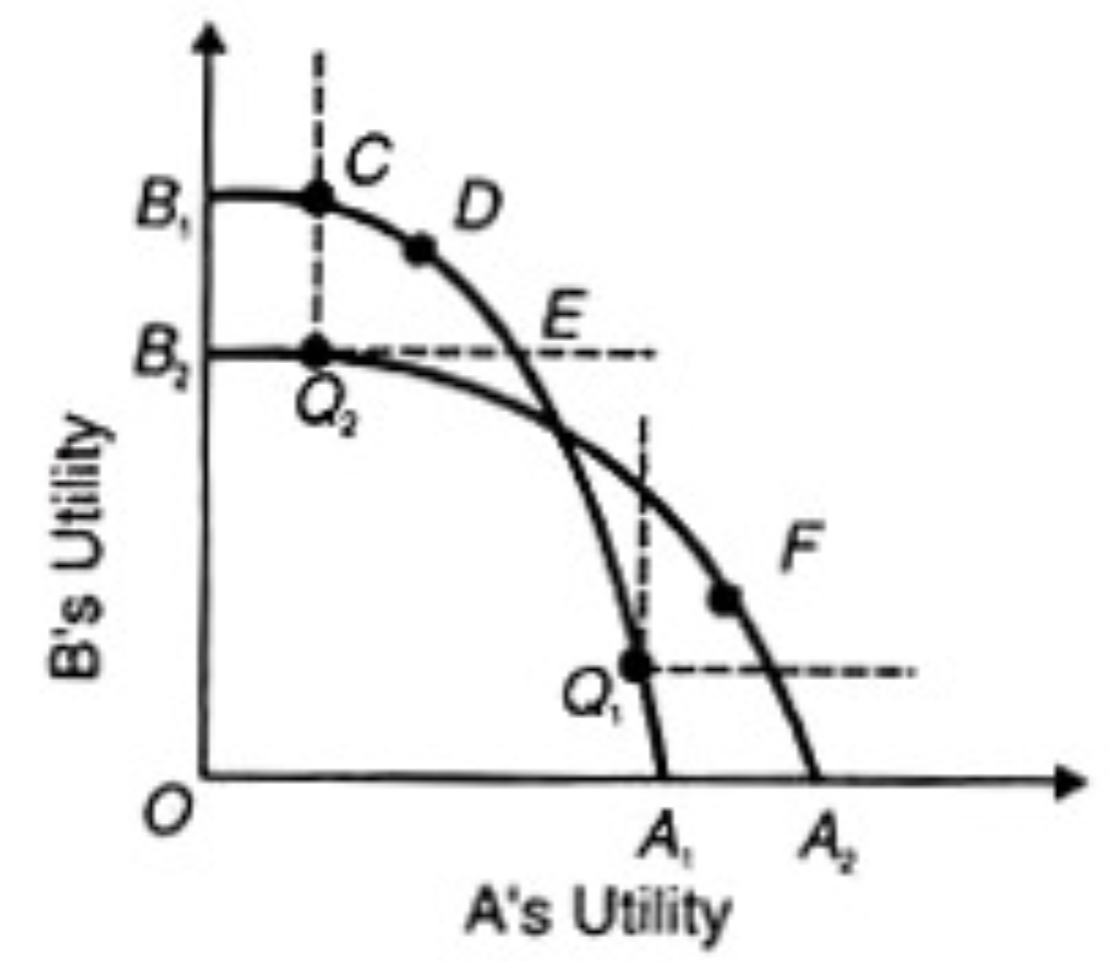
Figure 1: Comparison of ASW with CV: An illustration.

Figure 1 shows two allocations $Q_{1}$ and $Q_{2}$ with the utility possibility frontiers $A_{1}Q_{1}DB_{1}$ and $A_{2}FQ_{2}B_{2}$ through them intersecting. Each frontier represents the utility combinations attainable via redistribution between individuals A and B, starting from any point on it. Then the allocation $D$ Pareto dominates $Q_{2}$ and can be attained from $Q_{1}$ via redistribution. Therefore $Q_{1}$ is superior to $Q_{2}$ via the aggregate compensation principle. At the same time, the allocation $F$ which can be attained via redistribution from $Q_{2}$ is Pareto superior to $Q_{1}$, implying that $Q_{1}$ is inferior to $Q_{2}$ via the compensation principle; so aggregate CV is again negative, thus leading to an ambiguity. These conceptual shortcomings of the Hicksian approach have led instead to widespread use of the Bergson-Samuelson ASW criterion in applied research in public finance. In empirical IO, the widely used log-sum measure of consumer-welfare is precisely the ASW in the multinomial logit model, cf. Train 2003, Sec 3.5.

Quasilinear Utilities: If $U_{j}\left(y-p_{j},\eta\right)=h_{j}\left(\eta\right)+y-p_{j}$, and $U_{0}\left(y,\eta\right)=h_{0}\left(\eta\right)+y$, i.e. utility is quasilinear in the numeraire, then it can be shown (see appendix for derivation) that

$$W\left(\mathbf{p}^{1},y,\eta\right)-W\left(\mathbf{p}^{0},y,\eta\right)=-CV\left(y,\mathbf{p}^{0},\mathbf{p}^{1},\eta\right)\text{,}$$ (12)

and $W\left(\mathbf{p},y,\eta\right)$ equals

$$\left\{y+\max\left\{0,h_{1}\left(\eta\right)-p_{1}-h_{0}\left(\eta\right),...,h_{J}\left(\eta\right)-p_{J}-h_{0}\left(\eta\right)\right\}\right\}dF\left(\eta\right)\text{,}$$ (13)

so that the social marginal utility of income $\frac{\partial}{\partial y}\int W\left(\mathbf{p},y,\eta\right)dF\left(\eta\right)$ equals 1, which does not depend on $y$; i.e. society is indifferent between giving a dollar to a rich versus a poor individual. Thus aggregate CV gives a legitimate measure of social welfare when the social marginal utility of income is constant (cf. Blackorby and Donaldson 1988).

2.3 Binary Choice

Our application is a binary choice setting with $J=1$, where a subsidy on alternative 1 changes its price from $\bar{p}$ to $\bar{p}-\sigma$. In this case, the subsidy-induced change in average social welfare at income $y$ for a generic $\varepsilon\geq 0$ is given by

$$\Delta\left(\bar{p},\sigma,y;\varepsilon\right)\equiv\int_{0}^{\infty}\left(z+y\right)^{-\varepsilon}\times\left[q_{1}\left(\bar{p}-\sigma+z,y+z\right)-q_{1}\left(\bar{p}+z,y+z\right)\right]dz\text{;}$$ (14)

under $\varepsilon=0$, we have that

$$\Delta\left(\bar{p},\sigma,y;0\right)\equiv\int_{0}^{\infty}\left[q_{1}\left(\bar{p}-\sigma+z,y+z\right)-q_{1}\left(\bar{p}+z,y+z\right)\right]dz\text{;}$$ (15)

the average CV at income $y$ (cf. Bhattacharya 2015, eqn. 10) equals

$$S\left(\bar{p},\sigma,y\right)\equiv\int_{\bar{p}-\sigma}^{\bar{p}}q_{1}\left(p,y+p-\bar{p}+\sigma\right)dp\overset{\text{subs }z=p-\bar{p}+\sigma}{=}\int_{0}^{\sigma}q_{1}\left(\bar{p}-\sigma+z,y+z\right)dz\text{.}$$ (16)

Furthermore,

$$\int_{0}^{\infty}q_{1}\left(\bar{p}+z,y+z\right)dz\overset{\text{sub }t=z+\sigma}{=}\int_{\sigma}^{\infty}q_{1}\left(\bar{p}+t-\sigma,y+t-\sigma\right)dt$$ (17)

and therefore, from (15), (16) and (17) we have that

$$\Delta\left(\bar{p},\sigma,y;0\right)-S\left(\bar{p},\sigma,y\right)$$ (18)

$$= \int_{\sigma}^{\infty}\left[q_{1}\left(\bar{p}-\sigma+z,y+z\right)-q_{1}\left(\bar{p}-\sigma+z,y-\sigma+z\right)\right]dz$$

Now, the integrand in (18) is strictly positive (negative) for all $z$ if option 1 is normal (resp. inferior). Therefore, the only way $\Delta\left(\bar{p},\sigma,y;0\right)=S\left(\bar{p},\sigma,y\right)$ is that $q_{1}\left(p,y\right)$ does not depend on $y$, which implies utilities are quasilinear, and therefore by (13), the social marginal utility of income equals 1.

The average treatment effect, the quantity most commonly used in program evaluation and the treatment choice literature, equals

$$T\left(\bar{p},\sigma,y\right)\equiv q_{1}\left(\bar{p}-\sigma,y\right)-q_{1}\left(\bar{p},y\right)\text{,}$$ (19)

which is simply the integrand of (15) evaluated at the lower limit of the integral. Since this is measured as quantity of demand, a direct comparison with average or marginal subsidy cost is not possible. In contrast, the quantities $\Delta\left(\cdot,\cdot,\cdot\right)$ or $S\left(\cdot,\cdot,\cdot\right)$ provide theoretically justified monetary values of the choice, based on the choice-makers’ own preference.

Deadweight Loss (DWL): The average cost of the subsidy equals $\sigma\times q_{1}\left(\bar{p}-\sigma,y\right)$ in every case. Therefore, the DWL of the subsidy under $\varepsilon=0$ is given by

$$\sigma\times q_{1}\left(\bar{p}-\sigma,y\right)-\Delta\left(\bar{p},\sigma,y;0\right)$$ (20)

$$= \int_{\bar{p}-\sigma}^{\bar{p}}\left[q_{1}\left(\bar{p}-\sigma,y\right)-q_{1}\left(t,y+t-\bar{p}+\sigma\right)\right]dt$$

$$+\int_{\bar{p}}^{\infty}\left[q_{1}\left(t,y+t-\bar{p}\right)-q_{1}\left(t,y+t-\bar{p}+\sigma\right)\right]dt\text{.}$$

Note that the first term in (20) is positive because

$$q_{1}\left(t,y+t-\bar{p}+\sigma\right)-q_{1}\left(\bar{p}-\sigma,y\right)$$ (21)

$$= \Pr\left[U_{1}\left(y-\bar{p}+\sigma,\eta\right)\geq U_{0}\left(y+t-\bar{p}+\sigma,\eta\right)\right]-\Pr\left[U_{1}\left(y-\bar{p}+\sigma,\eta\right)\geq U_{0}\left(y,\eta\right)\right]$$

$$\leq 0\text{, for }t\geq\bar{p}-\sigma\text{ since }U_{0}\left(\cdot,\eta\right)\text{ is strictly increasing.}$$

The second term will be negative if the good is normal, and the DWL may be negative if the income effect is strongly positive. This is in contrast to the deadweight loss based on the CV which must necessarily be non-negative.

Finally, Hendren-Finkelstein’s MVPF at the status-quo ($p=\bar{p}$, $\sigma=0$) equals

$$\left.\frac{\frac{\partial}{\partial\sigma}\Delta\left(\bar{p},\sigma,y;0\right)}{\frac{\partial}{\partial\sigma}\left\{\sigma\times q_{1}\left(\bar{p}-\sigma,y\right)\right\}}\right|_{\sigma=0}\overset{\text{by (\ref{8a})}}{=}\frac{-\int_{0}^{\infty}\frac{\partial q_{1}\left(\bar{p}+z,y+z\right)}{\partial p}dz}{q_{1}\left(\bar{p},y\right)}$$ (22)

2.4 Treatment targeting

The constrained, optimal subsidy allocation problem takes the form

$$\max_{\sigma\left(\cdot\right)\in\mathcal{T}}\int B\left(\bar{p},\sigma\left(y\right),y\right)dF_{Y}\left(y\right)\text{ s.t. }\int\sigma\left(y\right)\times q_{1}\left(\bar{p}-\sigma\left(y\right),y\right)dF_{Y}\left(y\right)\leq M\text{,}$$ (23)

where $M$ denotes the planner’s budget constraint, $\mathcal{T}$ denotes the set of politically/practically feasible targeting rules, $F_{Y}\left(\cdot\right)$ is the marginal distribution of income in the population, and $B\left(\cdot,\cdot,\cdot\right)$ is one of $\Delta\left(\cdot,\cdot,\cdot\right)$, $S\left(\cdot,\cdot,\cdot\right)$ or $T\left(\cdot,\cdot,\cdot\right)$, defined in (15)-(19).

Parameter Uncertainty: Note that (23) seeks to maximize welfare of the individuals we observe. If instead, we treat our data as a random sample from a population, and wish to maximize welfare for that population, then we would need to take parameter uncertainty into account. This can be done by defining a loss function

$$L\left(\sigma\left(\cdot\right),\theta,c\right) = -\int B\left(\bar{p},\sigma\left(y\right),y,\theta\right)dF\left(y,\theta_{1}\right)$$ (24)

$$+c\left[M-\int\sigma\left(y\right)\times q_{1}\left(\bar{p}-\sigma\left(y\right),y,\theta_{2}\right)dF\left(y,\theta_{1}\right)\right]^{2}\text{,}$$

where $c$ denotes the penalty incurred by the planner from violating the budget constraint, and $\theta_{1}$, $\theta_{2}$ denote the parameters determining the marginal distribution of income and the demand function e.g. logit coefficients, respectively. Then define the optimal choice of $\sigma\left(\cdot\right)$ under a Bayesian criterion by solving

$$\min_{\sigma\left(\cdot\right)}\int L\left(\sigma\left(\cdot\right),\theta,c\right)dP_{post}\left(\theta|data\right)$$ (25)

where $P_{post}\left(\theta|data\right)$ refers to the posterior distribution of $\theta$ given the data. For computational simplicity, one can use the bootstrap distribution of $\theta$ to approximate the posterior corresponding to a flat prior (cf. Hastie et al 2009).

2.5 Identification and Estimation

Theorem 1 expresses the distribution of indirect utility in terms of the structural choice probability defined in (1). Learning the entire distribution of $W\left(\mathbf{p},y,\eta\right)$ at fixed $\mathbf{p},y$ would require one to estimate $q_{0}\left(c-y+p_{1},..c-y+p_{J},c\right)$ for all values of $c$. In any finite dataset, of course there will be limited variation of prices and income. So one can use a flexible parametric model such as random coefficients to estimate $q_{0}\left(c-y+p_{1},..c-y+p_{J},c\right)$ as is popular in empirical IO; shape restrictions on the choice probability functions (cf. Bhattacharya, 2021) can be imposed by restricting the support of the random coefficients. Any such parametric approximation would obviously impose additional restrictions on preference that are not required for Theorem 1 to hold. Alternatively, one can remain nonparametric and work with bounds. In particular,

$$q_{0}\left(c-y+p_{1},..c-y+p_{J},c\right)$$

$$= \Pr\left[U_{0}\left(c,\eta\right)\geq\max\left\{U_{1}\left(y-p_{1},\eta\right)...U_{J}\left(y-p_{J},\eta\right)\right\}\right]$$

and $U_{j}\left(\cdot,\eta\right)$ being strictly increasing for each $j$, yields nonparametric bounds on $q_{0}\left(c-y+p_{1},..c-y+p_{J},c\right)$. Specifically, let $S=\left\{\mathbf{r},z\right\}$ with $\mathbf{r=}\left(r_{1},...,r_{J}\right)$ be the set of price-income combinations observed in sample. Then lower and upper bounds on $q_{0}\left(c-y+p_{1},..c-y+p_{J},c\right)$ are given by

$$LB\left(c;\mathbf{p},y\right) = \max\left\{q_{0}\left(\mathbf{r},z\right):\left(\mathbf{r},z\right)\in S,\text{ }z-r_{j}\geq y-p_{j},\text{ }z\leq c\right\}$$

$$UB\left(c;\mathbf{p},y\right) = \min\left\{q_{0}\left(\mathbf{r},z\right):\left(\mathbf{r},z\right)\in S,\text{ }z-r_{j}\leq y-p_{j},\text{ }z\geq c\right\}\text{.}$$

Arguments presented in Bhattacharya 2021, Proposition 1 imply that these bounds are sharp.

Finally, if price and/or income are endogenous to individual preference, i.e. independence between utilities and budget set does not hold, then consistent estimation of $q_{0}$ would require the use of control function-type methods cf. Rivers-Vuong 1988, Newey 1987, Blundell-Powell 2004. We apply Newey’s approach in our empirical illustration below.

2.6 Ordered Discrete Choice and the Continuous Case

A result analogous to Theorem 1 does not hold for consumption of continuous goods such as gasoline (cf. Poterba, 1991) and food (Kochar 2005). To see why, consider the situation of ordered choice with 0 denoting the outside good and 1, 2 with unit price $p$ denoting the two inside good (e.g. no apple, 1 apple and 2 apples). Let the utilities be $U_{0}\left(y,\eta\right)$, $U_{1}\left(y-p,\eta\right)$, $U_{2}\left(y-2p,\eta\right)$. As above, normalize

$$W\left(p,y,\eta\right)\equiv\max\left\{y,U_{0}^{-1}\left(U_{1}\left(y-p,\eta\right),\eta\right),U_{0}^{-1}\left(U_{2}\left(y-2p,\eta\right),\eta\right)\right\}$$

Now, for $c\geq y$, we have that

$$\Pr\left[\max\left\{y,U_{0}^{-1}\left(U_{1}\left(y-p,\eta\right),\eta\right),U_{0}^{-1}\left(U_{2}\left(y-2p,\eta\right),\eta\right)\right\}\leq c\right]$$ (26)

$$= \Pr\left[\max\left\{U_{1}\left(y-p,\eta\right),U_{2}\left(y-2p,\eta\right)\right\}\leq U_{0}\left(c,\eta\right)\right]$$

$$= \Pr\left[\max\left\{U_{1}\left(c-\left(c-y+p\right),\eta\right),U_{1}\left(c-\left(c-y+2p\right),\eta\right)\right\}\leq U_{0}\left(c,\eta\right)\right]$$

$$= q_{0}\left(c-y+p,c-y+2p,c\right)\text{.}$$

But $q_{0}\left(c-y+p,c-y+2p,c\right)$ cannot be estimated, no matter how much $p$ and $y$ vary, because the data can only identify demand when the price of 2 units is twice the price of 1 unit; but $c-y+2p\neq 2\left(c-y+p\right)$. The continuous case can be thought of as the limiting case of ordered choice, e.g. one has to pay twice as much for 2 gallons of gasoline as for 1 gallon, and by the same logic, the welfare distribution for this case cannot be point-identified. One can however obtain bounds on (26) via

$$L\left(c;p,y\right)$$

$$\equiv \max\left\{q_{0}\left(\tilde{p},2\tilde{p},\tilde{y}\right):\tilde{y}-\tilde{p}\geq y-p,\tilde{y}-2\tilde{p}\geq y-2p,\tilde{y}\leq c\right\}$$

$$\leq \Pr\left[\max\left\{U_{1}\left(y-p,\eta\right),U_{2}\left(y-2p,\eta\right)\right\}\leq U_{0}\left(c,\eta\right)\right]$$

$$\equiv q_{0}\left(c-y+p,c-y+2p,c\right)$$

$$\leq \min\left\{q_{0}\left(\tilde{p},2\tilde{p},\tilde{y}\right):\tilde{y}-\tilde{p}\leq y-p,\tilde{y}-2\tilde{p}\leq y-2p,\tilde{y}\geq c\right\}$$

$$\equiv H\left(c;p,y\right)$$

and $L\left(c;p,y\right)$ and $H\left(c;p,y\right)$ are both potentially identifiable because they represent demand in situations where price of option 2 is twice the price of option 1. Note that $L\left(\cdot;p,y\right)$ and $H\left(\cdot;p,y\right)$ satisfy all properties of CDF’s.

3 Empirical Illustration: Private Tuition in India

Private, remedial tuition for children outside schools is ubiquitous in South Asia. Most of this is provided on a for-profit basis by school-teachers themselves. This creates perverse incentives for them to reduce their efforts inside the school classroom, cf. Jayachandran 2014. Thus children of richer households, who can afford the additional tuition-fees, benefit from the educational support outside school, whereas those from poorer households suffer the adverse consequences of lower-quality classroom-teaching. One possible way to address this problem is to tax private tuition for richer households and use the tax proceedings to subsidize poorer children. We investigate, empirically, the impact of this hypothetical policy intervention on social welfare, using the methods developed above.

Table 1: Application data summaries and welfare calculations.

Summary statistics.

Variable	Mean	St. dev.	Median	Min	Max
choice	0.4067	0.4912	0	0	1
price	3291.6	3689	2000	0	20000
monthly income (per household member)	9579.5	6379.2	8000	100	86700
household size	5.8799	2.4896	5	1	32
age of child	12.2658	3.5747	12	5	18
male	0.5395	0.4984	1	0	1

Welfare estimates.

Welfare quantity	At median income	Averaged over income
average compensating variation	1499.5	1501.8
	(30.056)	(31.531)
average treatment effect	0.0561	0.0561
	(0.0134)	(0.0135)
change in average social welfare, $\varepsilon=0$	1523.4	1520.9
	(281.822)	(279.252)
change in average social welfare, $\varepsilon=0.5$	10.51	10.43
	(1.681)	(1.672)
change in average social welfare, $\varepsilon=1$	0.0775	0.0787
	(0.0132)	(0.0136)

Welfare quantities in (15)-(19) calculated at $\bar{p}=4200$ (75th percentile of the price distribution), $\bar{p}-\sigma=900$ (25th percentile). Covariate values are at their median values. Bootstrap standard errors in parentheses are based on 400 replications.

We use micro-data from India’s National Sample Survey 71st round, conducted in January-June 2014. The key variables and summary statistics are reported in Table 1. Our sample size is 51092. There are two important data issues here. Firstly, if a household does not purchase private tuition, we do not observe their potential spending had they bought it. This is a well-known empirical issue in discrete choice applications; we address it by using the average price of those opting for private tuition in the village/block of the reference household to impute that price. An intuitive justification is that households are likely to base their decision on information they gather from acquaintances, and tuition-rates are unlikely to vary much within a neighborhood. A second issue, given that the data are non-experimental, is that prices are likely to be correlated with unobserved tuition-quality. We address this using ‘Hausman-instruments’ which are average price in other villages/blocks in the same strata (sampling areas larger than blocks but smaller than districts). The first-stage F-statistic has a p-value of $10^{-5}$.

We model demand for private tuition as

$$q_{1}(p,y)=\Phi\left(\beta_{p}p+\sum_{m=1}^{M}\beta_{y,m}\mathcal{R}_{m,M+q}(y;q)+x^{\prime}\beta\right),$$

where $p$ denotes price, $\mathcal{R}_{m,M+q}(y;q)$ are base B-splines of degree $q$ in monthly income $y$ and the covariate vector $x$ representing household size, the child’s age and sex. We use Newey’s (1987) two-step estimation approach that assumes joint normality of $u$ in the model for the latent variable

$$q_{1}^{\ast}=\beta_{p}p+\sum_{m=1}^{M}\beta_{y,m}\mathcal{R}_{m,M+q}(y;q)+x^{\prime}\beta+u$$

and the error in the reduced-form equation for price. To impose shape constraints, in the second step, we require

$$\beta_{p}\leq 0,$$

$$\beta_{p}+\sum_{m=2}^{M}\dfrac{\beta_{y,m}-\beta_{y,m-1}}{z_{m+q}-z_{m}}\mathcal{R}_{m-1,M+q-1}(y;q-1)\leq 0$$

with the second inequality imposed on a finite grid of income values. In the second inequality, $z_{m}$ denote knots on the support of income used in the construction of B-splines. The first (second) inequality guarantees that $q_{1}(p,y)$ is decreasing in price (in the direction $(1,1)$, i.e. $\frac{\partial}{\partial p}q_{1}(p,y)+\frac{\partial}{\partial y}q_{1}(p,y)\leq 0$ (cf. Bhattacharya 2021)).

The left of Figure 2 plots demand as a function of price for fixed income, and as a function of income for fixed price for a household with a representative set of characteristics. The inverted U-shape of the income graph agrees with widespread anecdotal evidence that academic success is primarily a middle-class aspiration in India, cf. Varma 2007.

The middle of Figure 2 shows the ACV and change in ASW, net of average cost, at median income and price over a range of subsides. We approximated the change in ASW at a given income value $y$ by calculating integrals in the definition of CASW from 0 to $y_{max}-y$, where $y_{max}$ denotes the largest observed income. This approximation is quite accurate as the values of integrands around $y_{max}-y$ are decreasing, taking values less than 0.0003. A negative subsidy is a tax, and the corresponding net-benefit equals the tax-revenue less utility-loss. We consider taxes up to 20% of median price and subsidy up to $Med(p)-\min(p)$. In the same figure, we plot the net-benefit approximation by the MVPF, i.e. $\sigma\times(numerator-demonominator)$ of (22). This curve is a straight line through the origin, showing the declining accuracy of first-order approximation as $\sigma$ rises.

The rightmost panel of Figure 2 shows the difference between ACV and change in ASW, when income-effects are/aren’t allowed.

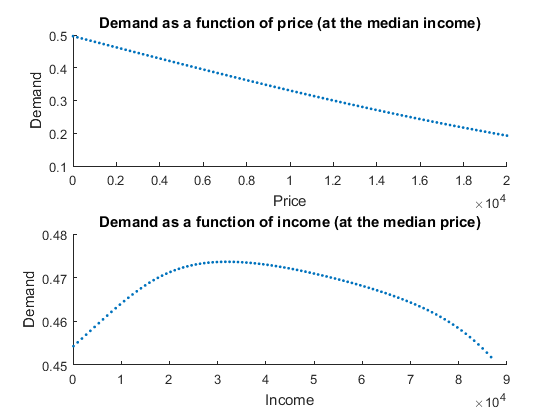
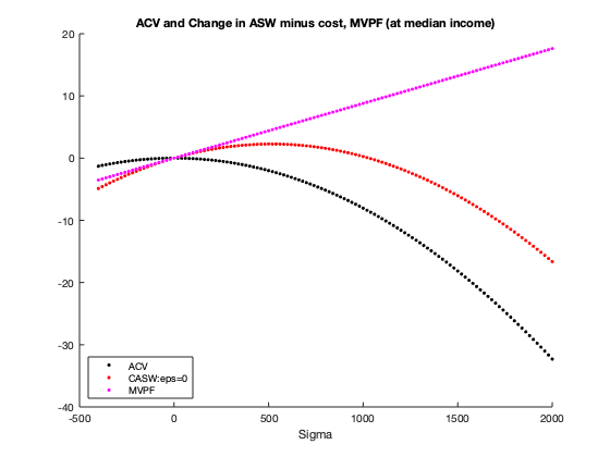
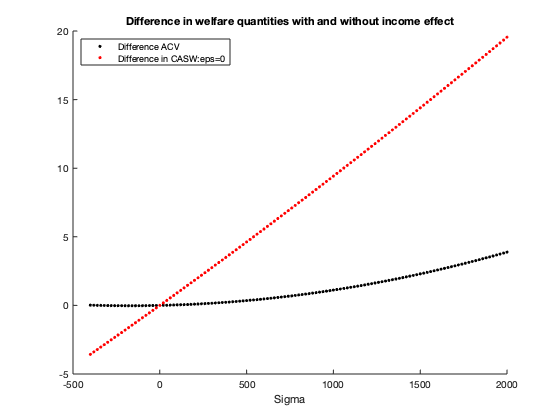
Figure 2: Left: Illustration of demand estimation. Middle: ACV, change in ASW ($\varepsilon=0$) net of average cost, and the first-order effect based on MVPF ($\bar{p}$ and $y$ are at their median levels). Covariate values are at their median levels. Right: Difference in ACV, change in ASW ($\varepsilon=0$) with and without income effect.

The income-effect is strong; consequently, the ACV and change in ASW curves differ substantially. Secondly, while deadweight loss for ACV is necessarily positive, that for the ASW is actually negative (benefit exceeds cost) over a range of income, which empirically illustrates our discussion around eqn. (21) above.

Table 1 reports changes in ASW for $\epsilon=0,0.5,1$, ACV and ATE calculated at $\bar{p}$ equal to the 75th percentile of the price distribution, $\bar{p}-\sigma$ equal to the 25th, covariates set equal to their median values, and $y$ set equal to median income $Med(y)$. We also include bootstrap standard errors.

A natural treatment-assignment problem in this case is to optimally subsidize the poor by taxing the rich in a budget-neutral way. The formal problem, analogous to (23) is

$$\max_{\sigma\left(\cdot\right)\in\mathcal{T}}\int B\left(\bar{p},\sigma\left(y\right),y\right)dF_{Y}\left(y\right)\text{ s.t. }\int\sigma\left(y\right)\times q_{1}\left(\bar{p}-\sigma\left(y\right),y\right)dF_{Y}\left(y\right)=0\text{,}$$ (27)

where $\mathcal{T}$ is now the space of spline functions which can take both positive and negative values. The optimal allocation where $B\left(\cdot,\cdot,\cdot\right)$ corresponds to average treatment-effect, change in ASW with $\varepsilon=0$ and average CV are shown in Figure 3.

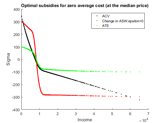
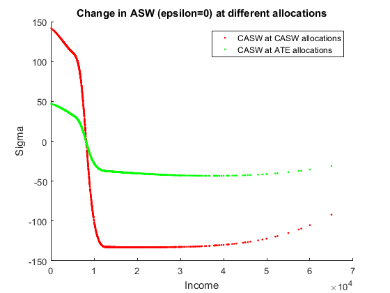
Figure 3: Left: Optimal subsidies for three different welfare criteria with the budget constraint giving the zero average cost. Right: Change in ASW ($\epsilon=0$) calculated at the CASW ($\epsilon=0$) optimal allocation path and at the ATE optimal allocation path.

Three features stand out. First, the allocation maximizing the ACV differs from the one that maximizes the CASW at $\epsilon=0$; this results from the large income-effect. Second, all three curves are downward sloping, because price-sensitivity of demand declines monotonically with income and the overall price-effect is much stronger than the income effect (see appendix Section 5.2.2 for details). Third, the ATE-maximizing allocation leads to the minimum disparity in subsidy/tax rates across the rich and poor, whereas maximizing the CASW leads to the highest disparity where the poor receive the highest subsidy and the rich face the highest tax. The optimal ACV curve lies in between.

The right panel in Figure 3 shows CASW when we use the ATE maximizing allocations compared to the CASW at the CASW-optimal allocations. Evidently, using the ATE-optimal allocation leads to much smaller redistribution of welfare from the rich to the poor, relative to the CASW-optimal allocation. Most of this operates at the intensive margin since the two graphs cross zero close to each other. That is, almost the same set of individuals sees an increase and decrease in their welfare in the two optimal allocations, but the extent of welfare-gain is much higher for the poor when using the CASW-optimal allocations. The figure looks somewhat similar to the optimal subsidy graph because the price-effect on demand – and, hence, aggregate welfare – is much stronger than the income-effect. At high incomes, demand becomes less price-sensitive, which explains why the similarity declines there.

For the alternative version that incorporates sampling uncertainty, the loss-function analogous to (24) is

$$L\left(\sigma\left(\cdot\right),\theta,c\right) = -\int B\left(\bar{p},\sigma\left(y\right),y,\theta_{1}\right)dF\left(y,\theta_{2}\right)$$ (28)

$$+c\left[\int\sigma\left(y\right)\times q_{1}\left(\bar{p}-\sigma\left(y\right),y,\theta_{1}\right)dF\left(y,\theta_{2}\right)\right]^{2}\text{,}$$

The optimal subsidy would solve (25) with this loss function (results not reported for brevity).

4 Conclusion

We show how to incorporate social welfare within traditional econometric program-evaluation and statistical treatment-assignment problems. Our main result pertains to the practically important setting of multinomial choice. The key insight is that the marginal distribution of suitably normalized individual indirect utility can be expressed as a closed-form functional of choice probabilities without functional-form assumptions on unobserved preference heterogeneity and income-effects. This leads to expressions for average weighted social welfare with weights reflecting planners’ distributional preferences and the optimal targeting of interventions that maximize aggregate utility under fixed budget. We discuss practical issues of identification and estimation, connections with and advantages relative to aggregate Hicksian welfare-measures, and potential extension to ordered and continuous choice. We illustrate our results using the example of private tuition demand in India where optimal, income-contingent targeting of subsidies/taxes leads to very different paths depending on whether average uptake or average social welfare is being maximized. The main source of this difference is how price-elasticity of demand varies with income.

References

1. Ahmad, E. and Stern, N., 1984. The theory of reform and Indian indirect taxes. Journal of Public economics, 25(3), pp.259-298.

2. Amemiya, T. 1978. The estimation of a simultaneous equation generalized probit model. Econometrica 46, pp.1193-1205.

3. Atkinson, A.B., 1970. On the measurement of inequality. Journal of economic theory, 2(3), 244-263.

4. Azam, M., 2016. Private tutoring: evidence from India. Review of Development Economics, 20(4), pp.739-761.

5. Banerjee, A., Niehaus, P. and Suri, T., 2019. Universal basic income in the developing world. Annual Review of Economics, 11, pp.959-983.

6. Banks, J., Blundell, R. and Lewbel, A., 1996. Tax reform and welfare measurement: do we need demand system estimation?. The Economic Journal, 106(438), 1227-1241.

7. Bergson, A., 1938. Reformulation of Certain Aspects of Welfare Economics. Quarterly Journal of Economics, 52.

8. Bhattacharya, D., 2015. Nonparametric welfare analysis for discrete choice. Econometrica, 83(2), pp.617-649.

9. Bhattacharya, D., 2018. Empirical welfare analysis for discrete choice: Some general results. Quantitative Economics, 9(2), pp.571-615.

10. Bhattacharya, D., 2021. The empirical content of binary choice models. Econometrica, 89(1), pp.457-474.

11. Bhattacharya, D. and P. Dupas, 2012. Inferring welfare maximizing treatment assignment under budget constraints, Journal of Econometrics, March 2012,167(1), 168–196.

12. Blackorby, C. and Donaldson, D., 1988. Money metric utility: A harmless normalization?. Journal of Economic Theory, 46(1), 120-129.

13. Blundell, R. and Powell, J.L., 2009. Endogeneity in nonparametric and semiparametric regression models, Chap 8 in Advances in Economics and Econometrics: Theory and Applications, Eighth World Congress, Cambridge University Press.

14. Blundell, R.W. and Powell, J.L., 2004. Endogeneity in semiparametric binary response models. The Review of Economic Studies, 71(3), pp.655-679.

15. Chetty, R., 2009. Sufficient statistics for welfare analysis: A bridge between structural and reduced-form methods. Annu. Rev. Econ., 1(1), pp.451-488.

16. Chipman, J. and Moore, J., 1990. Acceptable indicators of welfare change, consumer’s surplus analysis, and the Gorman polar form. Preferences, Uncertainty, and Optimality: Essays in Honor of Leonid Hurwicz, Westview Press, Boulder.

17. Cohen, J. and Dupas, P., 2010. Free distribution or cost-sharing? Evidence from a randomized malaria prevention experiment. Quarterly journal of Economics, 125(1).

18. De Boor, C. (1978). A practical guide to splines. New York, Springer-Verlag.

19. Deaton, A., 1984. Econometric issues for tax design in developing countries, reprinted in “The Theory of Taxation for Developing Countries”. Washington, DC: World Bank, 1987.

20. Dreze, J., 1998. Distribution matters in cost-benefit analysis: Comment on K.A. Brekke. Journal of Public Economics, 70(3), pp.485-488.

21. Dupas, P., 2014. Short-run subsidies and long-run adoption of new health products: Evidence from a field experiment. Econometrica, 82(1), pp.197-228.

22. Eilers, P.H. C. and Marx, B.D. (1996). Flexible Smoothing with $B$-splines and Penalties, Statistical Science, 11, pp. 89-102.

23. Einav, L., Finkelstein, A. and Cullen, M.R., 2010. Estimating welfare in insurance markets using variation in prices. The quarterly journal of economics, 125(3), pp.877-921.

24. Feldstein MS. 1999. Tax avoidance and the deadweight loss of the income tax. Rev. Econ. Stat, 81:674–80

25. Finkelstein, A. and Hendren, N., 2020. Welfare Analysis Meets Causal Inference, Journal of Economic Perspectives, vol. 34, no. 4, pp. 146-67.

26. Fleurbaey, M. and Hammond, P.J., 2004. Interpersonally comparable utility. In Handbook of utility theory (pp. 1179-1285). Springer, Boston, MA.

27. García, J.L. and Heckman, J.J., 2022. On criteria for evaluating social programs (No. w30005). National Bureau of Economic Research.

28. Goldberg, P.K. and Pavcnik, N., 2007. Distributional effects of globalization in developing countries. Journal of economic Literature, 45(1), pp.39-82.

29. Hammond, P.J., 1990. Interpersonal comparisons of utility: Why and how they are and should be made, European University Institute.

    https://cadmus.eui.eu/bitstream/handle/1814/342/1990_EUI%20WP_ECO_003.pdf?sequence=1

30. Hastie, T., Tibshirani, R., Friedman, J.H. and Friedman, J.H., 2009. The elements of statistical learning: data mining, inference, and prediction (Vol. 2, pp. 1-758). New York: springer.

31. Hausman, J. 1981. Exact Consumer’s Surplus and Deadweight Loss, The American Economic Review, Vol. 71, No. 4, 662-676.

32. Hausman JA. 1996. Valuation of new goods under perfect and imperfect competition. In The Economics of New Goods, eds. T. F. Bresnahan, RJ Gordon, chap. 5. Chicago: University of Chicago Press, 209–248.

33. Hausman, J.A. and Newey, W.K., 2016. Individual heterogeneity and average welfare. Econometrica, 84(3), pp.1225-1248.

34. Heckman, J.J. and Vytlacil, E.J., 2007. Econometric evaluation of social programs, part I: Causal models, structural models and econometric policy evaluation. Handbook of econometrics Vol. 6, 4779-4874.

35. Hendren, N. and Sprung-Keyser, B., 2020. A unified welfare analysis of government policies. The Quarterly Journal of Economics, 135(3), pp.1209-1318.

36. Herriges, J.A. and Kling, C.L., 1999. Nonlinear income effects in random utility models. Review of Economics and Statistics, 81(1), pp.62-72.

37. Imbens, G.W. and Wooldridge, J.M., 2009. Recent developments in the econometrics of program evaluation. Journal of economic literature, 47(1), pp.5-86.

38. Jayachandran, S., 2014. Incentives to teach badly: After-school tutoring in developing countries. Journal of Development Economics, 108, pp.190-205.

39. Kitagawa, T. and A. Tetenov 2018. Who Should Be Treated? Empirical Welfare Maximization Methods for Treatment Choice, Econometrica, 86(2), 591–616.

40. Kochar, A., 2005. Can targeted food programs improve nutrition? An empirical analysis of India’s public distribution system. Economic development and cultural change, 54(1), pp.203-235.

41. Luenberger, D.G., 1969. Optimization by vector space methods. John Wiley & Sons.

42. Mas-Colell, A., Whinston, M.D. and Green, J.R., 1995. Microeconomic theory (Vol. 1). New York: Oxford university press.

43. McFadden, D., 1981. Econometric models of probabilistic choice. Structural analysis of discrete data with econometric applications, 198272.

44. Manski, Charles F. 2004. Statistical Treatment Rules for Heterogeneous Populations, Econometrica, 72(4), 1221–1246.

45. Manski, C. F. 2014. Choosing size of government under ambiguity: Infrastructure spending and income taxation. The Economic Journal, 124(576), pp.359-376.

46. Mayshar, J., 1990. On measures of excess burden and their application. Journal of Public Economics, 43(3), pp.263-289.

47. McFadden, D. 1981, Econometric Models of Probabilistic Choice, in Manski and McFadden (eds.), Structural Analysis of Discrete Data with Econometric Applications, 198-272, MIT Press, Cambridge, Mass.

48. Mirrlees, J.A., 1971. An exploration in the theory of optimum income taxation. The review of economic studies, 38(2), pp.175-208.

49. Newey, W. K. 1987. Efficient estimation of limited dependent variable models with endogenous explanatory variables. Journal of Econometrics, 36, pp. 231-250.

50. Pollak, Robert A. ”Welfare comparisons and situation comparisons.” journal of Econometrics 50, no. 1-2 (1991): 31-48.

51. Poterba, J.M., 1991. Is the gasoline tax regressive?. Tax policy and the economy, 5, pp.145-164.

52. Ramsey, F.P., 1927. A Contribution to the Theory of Taxation. The Economic Journal, 37(145), 47-61.

53. Rivers, D., and Q. H. Vuong. 1988. Limited information estimators and exogeneity tests for simultaneous probit models. Journal of Econometrics 39, pp. 347-366.

54. Saez E. 2001. Using elasticities to derive optimal income tax rates. Rev. Econ. Stud. 68:205–29

55. Samuelson, P.A. 1947. Foundations of Economic Analysis, Ch. VIII, ”Welfare Economics”.

56. Scitovszky, T., 1941. A note on welfare propositions in economics. The Review of Economic Studies, 9(1), pp.77-88.

57. Sen, A.K. 1970. Collective Choice and Social Welfare. San Francisco: Holden-Day.

58. Slesnick, D.T., 1998. Empirical approaches to the measurement of welfare. Journal of Economic Literature, 36(4), pp.2108-2165.

59. Small, K.A. and Rosen, H.S., 1981. Applied welfare economics with discrete choice models. Econometrica: Journal of the Econometric Society, pp.105-130.

60. Smith, Richard J., and Richard W. Blundell. ”An exogeneity test for a simultaneous equation Tobit model with an application to labor supply.” Econometrica: journal of the Econometric Society (1986): 679-685.

61. Stern, N., 1987. The theory of optimal commodity and income taxation in The theory of taxation for developing countries, The World Bank.

62. Stifel, D. and Alderman, H., 2006. The “Glass of Milk” subsidy program and malnutrition in Peru. The World Bank Economic Review, 20(3), pp.421-448.

63. Varma, P.K., 2007. The great Indian middle class. Penguin Books India.

64. Tetenov, A., 2012. Statistical treatment choice based on asymmetric minimax regret criteria. Journal of Econometrics, 166(1), pp.157-165.

65. Train, K.E., 2009. Discrete choice methods with simulation. Cambridge university press.

66. Williams, H.C.W.L. 1977. On the Formulation of Travel Demand Models and Economic Measures of User Benefit, Environment & Planning A 9(3), 285-344.

5 Technical Appendix

Proof that CDF in Theorem 1 is non-decreasing:

Note that for $c^{\prime}>c\geq y$,

$$\Pr\left[W\left(\mathbf{p},y,\eta\right)\leq c^{\prime}\right]$$

$$= \bar{q}_{0}\left(c^{\prime}-y+p_{1},..c^{\prime}-y+p_{J},c^{\prime}\right)$$

$$= \Pr\left[\max\left\{U_{1}\left(c^{\prime}-\left(c^{\prime}-y+p_{1}\right),\eta\right),...,U_{J}\left(c^{\prime}-\left(c^{\prime}-y+p_{J}\right),\eta\right),\eta\right\}\leq U_{0}\left(c^{\prime},\eta\right)\right]$$

$$= \Pr\left[\max\left\{U_{1}\left(y-p_{1},\eta\right),...,U_{J}\left(y-p_{J},\eta\right),\eta\right\}\leq U_{0}\left(c^{\prime},\eta\right)\right]$$

$$\geq \Pr\left[\max\left\{U_{1}\left(y-p_{1},\eta\right),...,U_{J}\left(y-p_{J},\eta\right),\eta\right\}\leq U_{0}\left(c,\eta\right)\right]\text{, since }c^{\prime}>c\text{ and }U_{0}\left(\cdot,\eta\right)\nearrow$$

$$= \Pr\left[\max\left\{U_{1}\left(c-\left(c-y+p_{1}\right),\eta\right),...,U_{J}\left(c-\left(c-y+p_{J}\right),\eta\right),\eta\right\}\leq U_{0}\left(c,\eta\right)\right]$$

$$= \bar{q}_{0}\left(c-y+p_{1},..c-y+p_{J},c\right)$$

$$= \Pr\left[W\left(\mathbf{p},y,\eta\right)\leq c\right]\text{.}$$

For $y>c^{\prime}>c$, we have

$$\Pr\left[W\left(\mathbf{p},y,\eta\right)\leq c\right]=0=\Pr\left[W\left(\mathbf{p},y,\eta\right)\leq c^{\prime}\right]\text{,}$$

and finally, for $c^{\prime}\geq y>c$, we have

$$\Pr\left[W\left(\mathbf{p},y,\eta\right)\leq c\right] = 0$$

$$\leq \bar{q}_{0}\left(c^{\prime}-y+p_{1},..c^{\prime}-y+p_{J},c^{\prime}\right)=\Pr\left[W\left(\mathbf{p},y,\eta\right)\leq c^{\prime}\right]\text{.}$$

Proof of Assertion (11): Note that the move from $\mathbf{p}^{0}$ to $\infty_{J}$ can be decomposed into that from $\mathbf{p}^{0}$ to $\mathbf{p}^{1}$ and then from $\mathbf{p}^{1}$ to $\infty_{J}$, i.e.

$$CV\left(y,\mathbf{p}^{0},\infty_{J},\eta\right)$$

$$= CV\left(y,\mathbf{p}^{0},\mathbf{p}^{1},\eta\right)+CV\left(\underset{\neq y}{\underbrace{y+CV\left(y,\mathbf{p}^{0},\mathbf{p}^{1},\eta\right)}},\mathbf{p}^{1},\infty_{J},\eta\right)$$

$$\neq CV\left(y,\mathbf{p}^{0},\mathbf{p}^{1},\eta\right)+CV\left(y,\mathbf{p}^{1},\infty_{J},\eta\right)\text{,}$$

because $y+CV\left(y,\mathbf{p}^{0},\mathbf{p}^{1},\eta\right)\neq y$, and therefore (11) holds.

Quasilinear Utilities: If $U_{j}\left(y-p_{j},\eta\right)=h_{j}\left(\eta\right)+y-p_{j}$, and $U_{0}\left(y,\eta\right)=h_{0}\left(\eta\right)+y$, i.e. utility is quasilinear in the numeraire, then our normalization becomes $\mathcal{U}_{0}\left(y,\eta\right)=y$ and $\mathcal{U}_{j}\left(y-p_{j},\eta\right)=y+h_{j}\left(\eta\right)-h_{0}\left(\eta\right)-p_{j}$. Then

$$W\left(\infty_{J},y,\eta\right) = \mathcal{U}_{0}\left(y,\eta\right)=y\text{,}$$ (29)

$$W\left(\mathbf{p},y,\eta\right) = y+\max\left\{0,h_{1}\left(\eta\right)-p_{1}-h_{0}\left(\eta\right),...,h_{J}\left(\eta\right)-p_{J}-h_{0}\left(\eta\right)\right\}$$ (30)

Therefore,

$$y+\max\left\{0,h_{1}\left(\eta\right)-p_{10}-h_{0}\left(\eta\right),...,h_{J}\left(\eta\right)-p_{J0}-h_{0}\left(\eta\right)\right\}$$

$$= W\left(\mathbf{p}^{0},y,\eta\right)$$

$$= W\left(\mathbf{p}^{1},y+CV\left(y,\mathbf{p}^{0},\mathbf{p}^{1},\eta\right),\eta\right)$$

$$= \left[\begin{array}[]{l}y+CV\left(y,\mathbf{p}^{0},\mathbf{p}^{1},\eta\right)\\ +\max\left\{0,h_{1}\left(\eta\right)-p_{11}-h_{0}\left(\eta\right),...,h_{J}\left(\eta\right)-p_{J1}-h_{0}\left(\eta\right)\right\}\end{array}\right]\text{.}$$

Therefore,

$$CV\left(y,\mathbf{p}^{0},\mathbf{p}^{1},\eta\right)$$

$$= y+\max\left\{0,h_{1}\left(\eta\right)-p_{10}-h_{0}\left(\eta\right),...,h_{J}\left(\eta\right)-p_{J0}-h_{0}\left(\eta\right)\right\}$$

$$-\left(y+\max\left\{0,h_{1}\left(\eta\right)-p_{11}-h_{0}\left(\eta\right),...,h_{J}\left(\eta\right)-p_{J1}-h_{0}\left(\eta\right)\right\}\right)$$

$$= W\left(\mathbf{p}^{0},y,\eta\right)-W\left(\mathbf{p}^{1},y,\eta\right).$$

Thus, we have that under quasi-linear preferences,

$$W\left(\mathbf{p}^{1},y,\eta\right)-W\left(\mathbf{p}^{0},y,\eta\right)=-CV\left(y,\mathbf{p}^{0},\mathbf{p}^{1},\eta\right)\text{.}$$ (32)

Indeed, if utilities are quasilinear, then it follows that the social marginal utility of income $\frac{\partial\int W\left(\mathbf{p},y,\eta\right)dF\left(\eta\right)}{\partial y}$ equals

$$\frac{\partial}{\partial y}\int\left\{y+\max\left\{0,h_{1}\left(\eta\right)-p_{1}-h_{0}\left(\eta\right),...,h_{J}\left(\eta\right)-p_{J}-h_{0}\left(\eta\right)\right\}\right\}dF\left(\eta\right)=1\text{,}$$ (33)

which does not depend on $y$

5.1 Some details of demand estimation

Denote the support of $y$ as $[y_{min},y_{max}]$. Suppose we use B-splines of degree $q$ with $M+1$ equally spaced knots on $[y_{min},y_{max}]$ (including the end points). Each of the end points in the systems of knots enters with the multiplicity $q$. Then we have $M+q$ base B-splines which we denote as

$$\mathcal{R}_{m,M+q}(\cdot;q),\quad m=1,\ldots,M+q.$$

The definition of base B-splines through a recursive formula can be found, e.g., in de Boor 1978.

To incorporate covariates $x$ in the demand estimation, we collect all the covariates $x$ into an index $x^{\prime}\beta$ and specify the demand function as

$$P\left(q=1\,|\,p,y,x\right)=\Phi\left(+x^{\prime}\beta\right),$$

where $\Phi$ is the C.D.F. of the standard normal distribution. This specification automatically imposes normalization constraints on probability (that is, the probability varying between 0 and 1). Moreover, a monotonicity of this function in a direction of $(p,y)$ is equivalent to the respective monotonicity of $\beta_{p}p+\sum_{m=1}^{M}\beta_{y,m}\mathcal{R}_{m,M+q}(y;q)+x^{\prime}\beta$.

Using the well known formulas for the derivatives of B-splines (de Boor 1978), we obtain the following formulas for the derivative of $\sum_{m=1}^{M}\beta_{y,m}\mathcal{R}_{m,M+q}(y;q)$:

$$\dfrac{d\sum_{m=1}^{M}\beta_{y,m}\mathcal{R}_{m,M+q}(y;q)}{dy}=\sum_{m=2}^{M}\dfrac{\beta_{y.m}-\beta_{y,m-1}}{z_{m+q}-z_{m}}\mathcal{R}_{m-1,M+q-1}(y;q-1),$$

where $\mathcal{R}_{\tilde{m},M+q-1}(\cdot;q-1)$, $\tilde{m}=1,\ldots,M+q-1$, are base polynomials of degree $q-1$ constructed on the system of knots $\{z_{k}\},\;k=2,\ldots,M+2q$ (the multiplicity of each boundary knot is now reduced by 1).

5.2 Treatment Targeting Problem

5.2.1 Uniqueness and second order condition for treatment targeting problem

Uniqueness: In this part of the appendix, we clarify some intuition for why the optimal subsidy problem has a unique solution and the second order conditions for constrained maximum. It is easiest to see this in a simple setting where $Y$ takes 2 values $y_{1}$ and $y_{2}$ w.p. $\pi_{1}$ and $\pi_{2}$ respectively. Then the optimization problem becomes

$$\max_{\sigma_{1},\sigma_{2}}\pi_{1}B\left(\sigma_{1},y_{1}\right)+\pi_{2}B\left(\sigma_{2},y_{2}\right)$$

s.t.

$$\pi_{1}C\left(\sigma_{1},y_{1}\right)+\pi_{2}C\left(\sigma_{2},y_{2}\right)=M$$

To investigate uniqueness, first consider indifference maps for the benefit and cost functions. For benefits: let $B^{\prime}\left(\cdot\right)$ and $B^{\prime\prime}\left(\cdot\right)$ denote 1st and 2nd price derivative w.r.t. $\sigma$, then

$$\pi_{1}B\left(\sigma_{1},y_{1}\right)+\pi_{2}B\left(\sigma_{2},y_{2}\right) = const.$$

$$\Rightarrow \pi_{1}B^{\prime}\left(\sigma_{1},y_{1}\right)d\sigma_{1}+\pi_{2}B^{\prime}\left(\sigma_{2},y_{2}\right)d\sigma_{2}=0$$

$$\Rightarrow \left.\frac{d\sigma_{2}}{d\sigma_{1}}\right|_{B}=-\frac{\pi_{1}B^{\prime}\left(\sigma_{1},y_{1}\right)}{\pi_{2}B^{\prime}\left(\sigma_{2},y_{2}\right)}<0$$

$$\Rightarrow \left.\frac{d^{2}\sigma_{2}}{d\sigma_{1}^{2}}\right|_{B}=-\frac{\pi_{1}B^{{}^{\prime\prime}}\left(\sigma_{1},y_{1}\right)}{\pi_{2}B^{\prime}\left(\sigma_{2},y_{2}\right)}$$

Similarly, for costs, $C\left(\sigma_{1},y_{1}\right)=\sigma_{1}\times q\left(\bar{p}-\sigma_{1},y_{1}\right)$, let $C^{\prime}\left(\sigma_{1},y_{1}\right)$ and $C^{\prime\prime}\left(\sigma_{1},y_{1}\right)$ denote 1st and 2nd derivative w.r.t. $\sigma_{1}$. For indifference maps

$$\pi_{1}C\left(\sigma_{1},y_{1}\right)+\pi_{2}C\left(\sigma_{2},y_{2}\right) = const.$$

$$\Rightarrow \frac{d\sigma_{2}}{d\sigma_{1}}=-\frac{\pi_{1}C^{\prime}\left(\sigma_{1},y_{1}\right)}{\pi_{2}C^{\prime}\left(\sigma_{2},y_{2}\right)}<0$$

$$\Rightarrow \left.\frac{d^{2}\sigma_{2}}{d\sigma_{1}^{2}}\right|_{C}=-\frac{\pi_{1}C^{{}^{\prime\prime}}\left(\sigma_{1},y_{1}\right)}{\pi_{2}C^{\prime}\left(\sigma_{2},y_{2}\right)}$$

For the application, from the net benefit curves (i.e. benefit minus cost curves plotted against $\sigma$) we can obtain that

$$B^{\prime}\left(\sigma_{2},y_{2}\right)-C^{\prime}\left(\sigma_{2},y_{2}\right)<0\text{; \ }B^{{}^{\prime\prime}}\left(\sigma_{1},y_{1}\right)-C^{{}^{\prime\prime}}\left(\sigma_{1},y_{1}\right)<0.$$ (34)

From the benefit curves themselves we can get that $B^{\prime}\left(\sigma_{2},y_{2}\right)>0$, $B^{{}^{\prime\prime}}\left(\sigma_{1},y_{1}\right)>0$.

Putting all of this together, we have that

$$0 < B^{\prime}\left(\sigma_{2},y_{2}\right)<C^{\prime}\left(\sigma_{2},y_{2}\right)$$

$$0 < B^{{}^{\prime\prime}}\left(\sigma_{1},y_{1}\right)<C^{{}^{\prime\prime}}\left(\sigma_{1},y_{1}\right)$$

Therefore, from

$$\left.\frac{d^{2}\sigma_{2}}{d\sigma_{1}^{2}}\right|_{B}=-\frac{\pi_{1}B^{{}^{\prime\prime}}\left(\sigma_{1},y_{1}\right)}{\pi_{2}B^{\prime}\left(\sigma_{2},y_{2}\right)}\text{ and }\left.\frac{d^{2}\sigma_{2}}{d\sigma_{1}^{2}}\right|_{C}=-\frac{\pi_{1}C^{{}^{\prime\prime}}\left(\sigma_{1},y_{1}\right)}{\pi_{2}C^{\prime}\left(\sigma_{2},y_{2}\right)}\text{,}$$

we conclude that both indifference curves are decreasing and concave when viewed from the origin, with the benefit indifference curve less concave than the constant cost curve. Therefore there is a single internal maxima at the point where the benefit indifference curve is tangent to the cost indifference curve.

Second-order conditions: The ideas behind the second-order conditions for this case will extend to a general case. We write the Lagrangian as

$$\pi_{1}B\left(\sigma_{1},y_{1}\right)+\pi_{2}B\left(\sigma_{2},y_{2}\right)+\lambda\left(M-\pi_{1}C\left(\sigma_{1},y_{1}\right)+\pi_{2}C\left(\sigma_{2},y_{2}\right)\right).$$

The FOC is then

$$\pi_{1}B^{\prime}\left(\sigma_{1},y_{1}\right) = \lambda\pi_{1}C^{\prime}\left(\sigma_{1},y_{1}\right)\text{, }\;\pi_{2}B^{\prime}\left(\sigma_{2},y_{2}\right)=\lambda\pi_{2}C^{\prime}\left(\sigma_{2},y_{2}\right)$$

$$\Rightarrow \frac{B^{\prime}\left(\sigma_{1},y_{1}\right)}{C^{\prime}\left(\sigma_{1},y_{1}\right)}=\lambda=\frac{B^{\prime}\left(\sigma_{2},y_{2}\right)}{C^{\prime}\left(\sigma_{2},y_{2}\right)}.$$

The Bordered Hessian of the Lagrangian is

$$H = \left[\begin{array}[]{ccc}B^{\prime\prime}\left(\sigma_{1},y_{1}\right)-\lambda C^{\prime\prime}\left(\sigma_{1},y_{1}\right)&0&-\pi_{1}C^{\prime}\left(\sigma_{1},y_{1}\right)\\ 0&B^{\prime\prime}\left(\sigma_{2},y_{2}\right)-\lambda C^{\prime\prime}\left(\sigma_{2},y_{2}\right)&-\pi_{2}C^{\prime}\left(\sigma_{2},y_{2}\right)\\ -\pi_{1}C^{\prime}\left(\sigma_{1},y_{1}\right)&-\pi_{2}C^{\prime}\left(\sigma_{2},y_{2}\right)&0\end{array}\right]$$

$$= \left[\begin{array}[]{ccc}B^{\prime\prime}\left(\sigma_{1},y_{1}\right)-\frac{B^{\prime}\left(\sigma_{1},y_{1}\right)C^{\prime\prime}\left(\sigma_{1},y_{1}\right)}{C^{\prime}\left(\sigma_{1},y_{1}\right)}&0&-\pi_{1}C^{\prime}\left(\sigma_{1},y_{1}\right)\\ 0&B^{\prime\prime}\left(\sigma_{2},y_{2}\right)-\frac{B^{\prime}\left(\sigma_{2},y_{2}\right)C^{\prime\prime}\left(\sigma_{2},y_{2}\right)}{C^{\prime}\left(\sigma_{2},y_{2}\right)}&-\pi_{2}C^{\prime}\left(\sigma_{2},y_{2}\right)\\ -\pi_{1}C^{\prime}\left(\sigma_{1},y_{1}\right)&-\pi_{2}C^{\prime}\left(\sigma_{2},y_{2}\right)&0\end{array}\right]$$

For our solution to FOC to be a local maximizer, we need $\det H\left(\cdot\right)$ to be positive, i.e.

$$-\pi_{2}^{2}\left(C^{\prime}\left(\sigma_{2},y_{2}\right)\right)^{2}\times\left(B^{\prime\prime}\left(\sigma_{1},y_{1}\right)-\frac{B^{\prime}\left(\sigma_{1},y_{1}\right)C^{\prime\prime}\left(\sigma_{1},y_{1}\right)}{C^{\prime}\left(\sigma_{1},y_{1}\right)}\right)\\ -\pi_{1}^{2}\left(C^{\prime}\left(\sigma_{1},y_{1}\right)\right)^{2}\times\left(B^{\prime\prime}\left(\sigma_{2},y_{2}\right)-\frac{B^{\prime}\left(\sigma_{2},y_{2}\right)C^{\prime\prime}\left(\sigma_{2},y_{2}\right)}{C^{\prime}\left(\sigma_{2},y_{2}\right)}\right)>0.$$

Sufficient conditions for this are

$$\frac{B^{\prime\prime}\left(\sigma_{1},y_{1}\right)}{B^{\prime}\left(\sigma_{1},y_{1}\right)}<\frac{C^{\prime\prime}\left(\sigma_{1},y_{1}\right)}{C^{\prime}\left(\sigma_{1},y_{1}\right)},\quad\frac{B^{\prime\prime}\left(\sigma_{2},y_{2}\right)}{B^{\prime}\left(\sigma_{2},y_{2}\right)}<\frac{C^{\prime\prime}\left(\sigma_{2},y_{2}\right)}{C^{\prime}\left(\sigma_{2},y_{2}\right)}.$$

5.2.2 Shape of Optimal Subsidy as Function of Income

In this section we derive conditions that determine shapes of optimal ATE subsidies. In particular, we have a clear-cut condition of when these optimal subsidies as functions of income will be decreasing.

Suppose income $y$ takes 2 values $y_{1}<y_{2}$ w.p. $\pi_{1}$ and $\pi_{2}$ respectively. The expected ATE maximization problem becomes

$$\max_{\sigma_{1},\sigma_{2}}\pi_{1}q\left(\bar{p}-\sigma_{1},y_{1}\right)+\pi_{2}q\left(\bar{p}-\sigma_{2},y_{2}\right)$$

s.t.

$$\pi_{1}\sigma_{1}q\left(\bar{p}-\sigma_{1},y_{1}\right)+\pi_{2}\sigma_{2}q\left(\bar{p}-\sigma_{2},y_{2}\right)=M\text{.}$$

The Lagrangian is given by

$$\pi_{1}q\left(\bar{p}-\sigma_{1},y_{1}\right)+\pi_{2}q\left(\bar{p}-\sigma_{2},y_{2}\right)+\lambda\left(M-\pi_{1}\sigma_{1}q\left(\bar{p}-\sigma_{1},y_{1}\right)-\pi_{2}\sigma_{2}q\left(\bar{p}-\sigma_{2},y_{2}\right)\right)$$

yielding FOC

$$-\pi_{1}\frac{\partial}{\partial p}q\left(\bar{p}-\sigma_{1},y_{1}\right) = \lambda\pi_{1}\left(q\left(\bar{p}-\sigma_{1},y_{1}\right)-\sigma_{1}\frac{\partial}{\partial p}q\left(\bar{p}-\sigma_{1},y_{1}\right)\right)$$ (37)

$$-\pi_{2}\frac{\partial}{\partial p}q\left(\bar{p}-\sigma_{2},y_{2}\right) = \lambda\pi_{2}\left(q\left(\bar{p}-\sigma_{2},y_{2}\right)-\sigma_{2}\frac{\partial}{\partial p}q\left(\bar{p}-\sigma_{2},y_{2}\right)\right)$$ (38)

Taking ratios and using $\eta_{1}\left(\bar{p},\sigma_{1},y_{1}\right)\equiv-\frac{\frac{\partial}{\partial p}q\left(\bar{p}-\sigma_{1},y_{1}\right)}{q\left(\bar{p}-\sigma_{1},y_{1}\right)}>0$, we get

$$\frac{\frac{\partial}{\partial p}q\left(\bar{p}-\sigma_{1},y_{1}\right)}{\frac{\partial}{\partial p}q\left(\bar{p}-\sigma_{2},y_{2}\right)} = \frac{q\left(\bar{p}-\sigma_{1},y_{1}\right)-\sigma_{1}\frac{\partial}{\partial p}q\left(\bar{p}-\sigma_{1},y_{1}\right)}{q\left(\bar{p}-\sigma_{2},y_{2}\right)-\sigma_{2}\frac{\partial}{\partial p}q\left(\bar{p}-\sigma_{2},y_{2}\right)}$$

$$\Longrightarrow \frac{\frac{\frac{\partial}{\partial p}q\left(\bar{p}-\sigma_{1},y_{1}\right)}{q\left(\bar{p}-\sigma_{1},y_{1}\right)}}{\frac{\frac{\partial}{\partial p}q\left(\bar{p}-\sigma_{2},y_{2}\right)}{q\left(\bar{p}-\sigma_{2},y_{2}\right)}}=\frac{1-\sigma_{1}\frac{\frac{\partial}{\partial p}q\left(\bar{p}-\sigma_{1},y_{1}\right)}{q\left(\bar{p}-\sigma_{1},y_{1}\right)}}{1-\sigma_{2}\frac{\frac{\partial}{\partial p}q\left(\bar{p}-\sigma_{2},y_{2}\right)}{q\left(\bar{p}-\sigma_{2},y_{2}\right)}}$$

$$\Longrightarrow \frac{\eta_{1}}{\eta_{2}}=\frac{1+\sigma_{1}\eta_{1}}{1+\sigma_{2}\eta_{2}}$$

$$\Longrightarrow \eta_{1}\left(1+\sigma_{2}\eta_{2}\right)=\left(1+\sigma_{1}\eta_{1}\right)\eta_{2}$$

$$\Longrightarrow \eta_{1}+\sigma_{2}\eta_{2}\eta_{1}=\eta_{2}+\sigma_{1}\eta_{1}\eta_{2}$$

$$\Longrightarrow \left(\sigma_{2}-\sigma_{1}\right)\eta_{2}\eta_{1}=\eta_{2}-\eta_{1}$$

$$\Longrightarrow \sigma_{2}-\sigma_{1}=\frac{\eta_{2}-\eta_{1}}{\eta_{2}\eta_{1}}=\frac{1}{\eta_{1}}-\frac{1}{\eta_{2}}$$ (40)

The above inequality is consistent with $\sigma_{2}<\sigma_{1}$ (i.e. subsidy is progressive) if and only if $\eta_{2}<\eta_{1}$, i.e.

$$\left|\frac{\frac{\partial}{\partial p}q\left(\bar{p}-\sigma_{1},y_{1}\right)}{q\left(\bar{p}-\sigma_{1},y_{1}\right)}\right|>\left|\frac{\frac{\partial}{\partial p}q\left(\bar{p}-\sigma_{2},y_{2}\right)}{q\left(\bar{p}-\sigma_{2},y_{2}\right)}\right|$$ (41)

for $y_{1}<y_{2}$ and $\sigma_{2}<\sigma_{1}$, i.e. the price sensitivity of demand measured by $\left.\left|\frac{\partial}{\partial p}\ln q\left(p,y\right)\right|\right|_{p=\tilde{p},y=\tilde{y}}$ is decreasing in $\tilde{y}$ at fixed $\tilde{p}$ and is increasing in $\tilde{p}$ for fixed $\tilde{y}$. The derivations here clearly extend from two to multiple possible values of income.

For the application, Figure 4 depicts the absolute values of the derivatives $\left.\left|\frac{\partial}{\partial p}\ln q\left(p,y\right)\right|\right|$ as functions of incomes (for incomes from the 3rd till the 97th percentile) at different price percentiles (even though $\bar{p}$ is the median price, since the subsidy can be negative, we consider percentiles above the median). These absolute values are decreasing in $y$ and, moreover, there is an ordering of the curves with respect to price percentiles. Therefore, the optimal ATE subsidy cannot be increasing in $y$. Indeed, suppose it increased when we moved from $y_{1}$ to $y_{2}$, where $y_{2}>y_{1}$. This would mean that we would move to a lower curve and, due to the decreasing nature of each curve, the inequality in (41) would hold, which leads to a contradiction. Therefore, the optimal ATE subsidy is decreasing in income, as illustrated in Figure 3. Because of the consistent shape pattern of curves across the incomes, similar findings apply also CASW and ACV criteria.

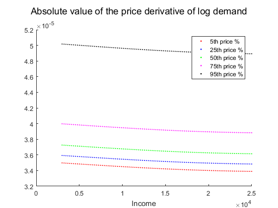
Figure 4: Private tuition application. Absolute values of the derivatives $\left.\left|\frac{\partial}{\partial p}\ln q\left(p,y\right)\right|\right|$ as functions of incomes (for incomes from the 3rd till the 97th percentile) at different price percentiles.