Minimal angle spread in the probability simplex
with respect to the uniform distribution

Abstract

We compute the minimal angle spread with respect to the uniform distribution in the probability simplex. The resulting optimization problem is analytically solved. The formula provided shows that the minimal angle spread approaches zero as the dimension tends to infinity. We also discuss an application in cognitive science.

1 Introduction

Throughout this paper, we assume that

(1) $$X:=\mathbb{R}^{n} \left\langle{\cdot},{\cdot}\right\rangle\colon X\times X\to\mathbb{R}$$ with inner product ,

and induced Euclidean norm $\|\cdot\|$. We also define the probability simplex by

(2) $$\Delta:=\Delta_{n}:=\big{\{}{(x_{1},\ldots,x_{n})\in\mathbb{R}^{n}_{+}}~{}\big{|}~{}{x_{1}+x_{2}+\cdots+x_{n}=1}\big{\}},$$

where $\mathbb{R}_{+}=\big{\{}{x\in\mathbb{R}}~{}\big{|}~{}{x\geq 0}\big{\}}$. The probability simplex is of central importance in Statistics, Optimization, and Information Theory; see, e.g., [4] and [11]. (We write $\Delta_{n}$ if we wish to emphasize the dimension $n$.) It will be convenient to set

(3) $$\boldsymbol{1}:=(1,1,\ldots,1)\in\mathbb{R}^{n}\quad\text{and}\quad u:=\big{(}\tfrac{1}{n},\tfrac{1}{n},\ldots,\tfrac{1}{n}\big{)}\in\Delta_{n}.$$

The problem we investigate is the following: Given $p\in\Delta\smallsetminus\{u\}$, there exist two unique points $a=a(p)$ and $b=b(p)$ in $\Delta$ such that $\{u,p\}\subseteq[a,b]$ and $\|a-b\|$ is maximal. (Let us note that when, e.g., $n=3$, then the mapping $\Delta\smallsetminus\{u\}\colon\mathbb{R}\colon p\mapsto\|a(p)-b(p)\|$ is continuous; however, it is not possible to extend it continuously — let alone in a smooth manner — at the point $u$.) The quantity $\|a-b\|$ can be thought of as the “width“ of $\Delta$ with respect to $p$ and

(4) $$\cos\big{(}\measuredangle(a,b)\big{)}=\frac{\left\langle{a},{b}\right\rangle}{\|a\|\|b\|}$$

as the cosine of the “angle spread” with respect to $p$.

The aim of this paper is to minimize the angle spread, which equivalently corresponds to maximizing its cosine

(P) $$\max_{p\in\Delta\smallsetminus\{u\}}{\frac{\left\langle{a(p)},{b(p)}\right\rangle}{\|a(p)\|\|b(p)\|}}.$$

When $n=2$, it is clear that the maximum value of Eq. P is $\cos(\pi/2)=0$ and that every $p\in\Delta\smallsetminus\{u\}$ solves Eq. P. Thus, we assume henceforth that

(5) $$n\in\{3,4,\ldots\}.$$

Our main result can now be stated:

Theorem 1.1.

The maximum value of Eq. P is

(6) $$\frac{n-2}{n+2}$$

and a pair realizing this maximum is $a^{*}=\tfrac{1}{n}(2,1,1,\ldots,1,0)$ and $b^{*}=\tfrac{1}{n}(0,1,1,\ldots,1,2)$. Consequently, the minimal angle spread is

(7) $$\arccos\Big{(}\frac{n-2}{n+2}\Big{)}.$$

See Fig. 1 for an illustration of Theorem 1.1 when $n=3$. We note that as the dimension of the space $n$ increases to infinity, the minimal angle spread approaches $\arccos(1)=0$. We also note that when $n=1,2,4$, then $\pi-\arccos((n-2)/(n+2))$ coincides with the dihedral angle of the tetrahedron, cube, octahedron, respectively. However, dihedral angles of other classical polyhedra (see [16]) do not seem to be related to the angles provided by Eq. 7.

Our strategy to prove Theorem 1.1 is to reduce the complexity of the problem in stages by exploiting its structure. Eventually, we are led to a one-dimensional problem which we then solve by Calculus.

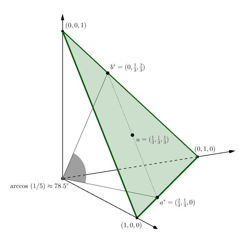
Figure 1: An illustration of Theorem 1.1 when $n=3$.

The remainder of this paper is organized as follows. In Section 2, we collect a technical optimization result that will be used later. The computation of $[a,b]$ is carried out in Section 3. In Section 4, we set up the cosine quotient Eq. 4 in a more tractable form. The optimization is then tackled in Section 5 where we keep $p_{1}$ and $p_{n}$ fixed. At last, the proof is completed in Section 6. In Section 7, we sketch an application of our results — which in fact motivated this note — in cognitive science. The presented results are a first contribution to using the minimal angle spread as a nonsmooth discrepancy term in this area.

Finally, we note that a reviewer pointed out that another possible departure point is to study sufficient conditions for strong convexity of integral functionals in two-stage stochastic linear programming. In particular, recent work by Claus and Spürkel [3] features minimal angles of similar though different kind. This is a promising direction to explore in future research.

The notation in this paper is fairly standard and follows largely [1].

2 An auxiliary result

It will be convenient to have the following result ready for future use.

Lemma 2.1.

Let $m\in\{1,2,\ldots\}$, set $\boldsymbol{1}:=(1,1,\ldots,1)\in\mathbb{R}^{m}$, and let $\gamma\in\mathbb{R}$. Set $h\colon\mathbb{R}^{m}\to\mathbb{R}_{+}\colon x\mapsto\|x-\gamma\boldsymbol{1}\|^{2}$, let $x\in\mathbb{R}^{m}$, and set

$$y:=(\eta,\eta,\ldots,\eta)\in\mathbb{R}^{m},\quad\text{where}\quad\eta:=\tfrac{1}{m}(x_{1}+x_{2}+\cdots+x_{m}).$$

Then

$$h(y)\leq h(x).$$

Proof 2.2.

Indeed, we have

$$h(y)-\gamma^{2}\|\boldsymbol{1}\|^{2} =\|y\|^{2}-2\gamma\left\langle{y},{\boldsymbol{1}}\right\rangle=m\eta^{2}-2\gamma m\eta$$

$$=m\big{(}\tfrac{1}{m}(x_{1}+x_{2}+\cdots+x_{m})\big{)}^{2}-2\gamma(x_{1}+x_{2}+\cdots+x_{m})$$

$$\leq m\tfrac{1}{m}\big{(}x_{1}^{2}+x_{2}^{2}+\cdots+x_{m}^{2}\big{)}-2\gamma\left\langle{x},{\boldsymbol{1}}\right\rangle$$

$$=\|x\|^{2}-2\gamma\left\langle{x},{\boldsymbol{1}}\right\rangle$$

$$=h(x)-\gamma^{2}\|\boldsymbol{1}\|^{2},$$

where the inequality follows from the convexity of the square function.

Corollary 2.3.

Let $m\in\{1,2,\ldots\}$, and let $\gamma\in\mathbb{R}$. Set $A\colon\mathbb{R}^{m}\to\mathbb{R}^{m}\colon x\mapsto(\eta,\eta,\ldots,\eta)$, where $\eta=\tfrac{1}{m}(x_{1}+x_{2}+\cdots+x_{m})$, and let $C$ be a nonempty subset of $\mathbb{R}^{m}$ such that $A(C)\subseteq C$. Set $\boldsymbol{1}:=(1,1,\ldots,1)\in\mathbb{R}^{m}$. Then to

(8) $$\text{minimize}\;\;\|x-\gamma\boldsymbol{1}\|^{2}\;\;\text{over $x\in C$}$$

is the same as to

(9) $$\text{minimize}\;\;\|x-\gamma\boldsymbol{1}\|^{2}\;\;\text{over $x\in C\cap\mathbb{R}\,\boldsymbol{1}$}$$

in the sense that the optimal values for both problems are identical and if the first problem has a solution, then it also has a solution that solves also the second problem.

Proof 2.4.

Clear from Lemma 2.1.

Remark 2.5.

We point out in passing that the operator $A$ from Corollary 2.3 is the projection operator of the set $\mathbb{R}\boldsymbol{1}$.

3 Determining the relative boundary points $\scriptstyle a$ and $\scriptstyle b$

In this section, we fix

(10) $$p\in\Delta\smallsetminus\{u\}.$$

Then there exist indices $i$ and $j$ in $I:=\{1,2,\ldots,n\}$ such that $p_{i}<\tfrac{1}{n}<p_{j}$. Without loss of generality, we assume that

(11) $$0\leq p_{1}=\min_{i\in I}p_{i}<\tfrac{1}{n}<p_{n}=\max_{i\in I}p_{i}\leq 1.$$

Set

(12) $$(\forall\lambda\in\mathbb{R})\quad q(\lambda):=(1-\lambda)u+\lambda p=u+\lambda(p-u).$$

Note that $q(0)=u$, $q(1)=p$,

(13) $$(\forall\lambda\in\mathbb{R})(\forall i\in I)\quad q_{i}(\lambda)=(1-\lambda)u_{i}+\lambda p_{i}=u_{i}+\lambda(p_{i}-u_{i}),$$

and hence

(14) $$q_{1}(\lambda)+q_{2}(\lambda)+\cdots+q_{n}(\lambda)=1.$$

We wish to find the smallest and largest $\lambda\in\mathbb{R}$ such that $q(\lambda)\in\Delta$. Let $i\in I$. Suppose that $p_{i}>u_{i}$. Then $(\forall\lambda\in\mathbb{R}_{+})$ $q_{i}(\lambda)>u_{i}$. So if $\lambda<0$, then $q_{i}(\lambda)=0$ $\Leftrightarrow$ $-u_{i}=\lambda(p_{i}-u_{i})$ $\Leftrightarrow$ $\lambda=-u_{i}/(p_{i}-u_{i})=-(1/n)/(p_{i}-(1/n))=-1/(np_{i}-1)\leq-1/(np_{n}-1)$. Hence the smallest value $\lambda$ still guaranteeing $q(\lambda)\in\Delta$ is

(15) $$\lambda_{-}:=\frac{-1}{np_{n}-1}=\frac{1}{1-np_{n}}<0.$$

Analogously, the largest value $\lambda$ still guaranteeing $q(\lambda)\in\Delta$ is

(16) $$\lambda_{+}:=\frac{1}{1-np_{1}}>0.$$

The corresponding vectors

(17) $$a:=q(\lambda_{-})=u+\lambda_{-}(p-u)$$

and

(18) $$b:=q(\lambda_{+})=u+\lambda_{+}(p-u)$$

thus form the largest segment $[a,b]\subseteq\Delta$ such that $\{u,p\}\subseteq[a,b]$. Note that $a$ and $b$ are depending on $p$ — when we want to stress this, then we’ll write $a(p)$ and $b(p)$.

For $i\in I$, we simplify

(19) $$a_{i}=u_{i}+\lambda_{-}(p_{i}-u_{i})=\tfrac{1}{n}+\frac{1}{1-np_{n}}\big{(}p_{i}-\tfrac{1}{n}\big{)}=\frac{1-np_{n}+n\big{(}p_{i}-\tfrac{1}{n}\big{)}}{n(1-np_{n})}=\frac{p_{n}-p_{i}}{np_{n}-1}$$

and similarly

(20) $$b_{i}=\frac{p_{i}-p_{1}}{1-np_{1}}.$$

Thus

(21) $$a=\frac{1}{np_{n}-1}(p_{n}\boldsymbol{1}-p)\;\;\text{and}\;\;b=\frac{1}{1-np_{1}}(p-p_{1}\boldsymbol{1}),$$

where $\boldsymbol{1}=(1,1,\ldots,1)\in\mathbb{R}^{n}$. Next,

(22a) $$\|a\|^{2} =\frac{1}{(np_{n}-1)^{2}}\|p_{n}\boldsymbol{1}-p\|^{2}=\frac{1}{(np_{n}-1)^{2}}\big{(}p_{n}^{2}\|\boldsymbol{1}\|^{2}-2p_{n}\left\langle{\boldsymbol{1}},{p}\right\rangle+\|p\|^{2}\big{)}$$

(22b) $$=\frac{1}{(np_{n}-1)^{2}}\big{(}np_{n}^{2}-2p_{n}+\|p\|^{2}\big{)}$$

(22c) $$=\frac{1}{(np_{n}-1)^{2}}\Big{(}p_{1}^{2}+\big{(}p_{2}^{2}+\cdots+p_{n-1}^{2}\big{)}+(n+1)p_{n}^{2}-2p_{n}\Big{)}$$

and similarly

(23) $$\|b\|^{2}=\frac{1}{(1-np_{1})^{2}}\Big{(}(n+1)p_{1}^{2}-2p_{1}+\big{(}p_{2}^{2}+\cdots+p_{n-1}^{2}\big{)}+p_{n}^{2}\Big{)}.$$

4 Setting up the cosine quotient

We uphold the assumptions and notation from the previous section. It is convenient to abbreviate

(24) $$z:=(p_{2},\ldots,p_{n-1})\in\mathbb{R}^{n-2}.$$

Note that

(25) $$(\forall i\in\{1,2,\ldots,n-2\})\;\;p_{1}\leq z_{i}\leq p_{n}\quad\text{and}\quad\sum_{i=1}^{n-2}z_{i}=1-p_{1}-p_{n}\geq 0$$

because of Eq. 10 and Eq. 11. This allows us to rewrite Eq. 22 and Eq. 23 more succinctly as

(26) $$\|a\|^{2}=\frac{1}{(np_{n}-1)^{2}}\big{(}p_{1}^{2}+\|z\|^{2}+(n+1)p_{n}^{2}-2p_{n}\big{)}$$

and

(27) $$\|b\|^{2}=\frac{1}{(1-np_{1})^{2}}\big{(}(n+1)p_{1}^{2}-2p_{1}+\|z\|^{2}+p_{n}^{2}\big{)}.$$

Next, using Eq. 19 and Eq. 20, we have

(28a) $$\left\langle{a},{b}\right\rangle =\sum_{i=1}^{n}a_{i}b_{i}=\sum_{i=1}^{n}\frac{p_{n}-p_{i}}{np_{n}-1}\cdot\frac{p_{i}-p_{1}}{1-np_{1}}$$

(28b) $$=\frac{1}{(np_{n}-1)(1-np_{1})}\sum_{i=2}^{n-1}(p_{n}-p_{i})(p_{i}-p_{1})$$

(28c) $$=\frac{1}{(np_{n}-1)(1-np_{1})}\sum_{i=1}^{n-2}(p_{n}-z_{i})(z_{i}-p_{1}).$$

Using Eq. 28, Eq. 26, and Eq. 27, we now set up the quotient of interest from Eq. 4:

(29) $$\frac{\left\langle{a},{b}\right\rangle}{\|a\|\|b\|}=\frac{\displaystyle\sum_{i=1}^{n-2}(p_{n}-z_{i})(z_{i}-p_{1})}{\sqrt{p_{1}^{2}+\|z\|^{2}+(n+1)p_{n}^{2}-2p_{n}}\sqrt{(n+1)p_{1}^{2}-2p_{1}+\|z\|^{2}+p_{n}^{2}}}.$$

5 Maximizing the cosine quotient (with $\scriptstyle p_{1}$ and $\scriptstyle p_{n}$ fixed)

We uphold the notation of the previous section. Now we turn toward maximizing the cosine quotient Eq. 29, with $p_{1}$ and $p_{n}$ fixed. In view of Eq. 25, $z=(p_{2},\ldots,p_{n-1})$ must belong to the compact convex set

(30) $$C:=\bigg{\{}{w\in[p_{1},p_{n}]^{n-2}}~{}\bigg{|}~{}{\sum_{i=1}^{n-2}w_{i}=1-p_{1}-p_{n}}\bigg{\}}.$$

The continuity of Eq. 29 as a function of $z$ coupled with the compactness of $C$ guarantees the existence of a maximizer of the cosine quotient. Note that

(31) $$A(C)\subseteq C,$$

where $A\colon\mathbb{R}^{n-2}\to\mathbb{R}^{n-2}\colon w\mapsto(\eta,\eta,\ldots,\eta)\in\mathbb{R}^{n-2}$ and $\eta=\tfrac{1}{n-2}(w_{1}+w_{2}+\cdots+w_{n-2})$.

In general, maximizing a quotient is more involved; however, we will get a lucky break for our problem: It turns out we can maximize the numerator and minimize the denominator of Eq. 29 with respect to $z$ and we luckily obtain the same optimal vector!

For convenience, set $\alpha:=p_{1}$, $\beta:=p_{n}$, $\gamma:=(\alpha+\beta)/2$, and $\boldsymbol{1}:=(1,1,\ldots,1)\in\mathbb{R}^{n-2}$. Then the numerator of Eq. 29 — as a function of $z$ — is

(32a) $$\sum_{i=1}^{n-2}(\beta-z_{i})(z_{i}-\alpha) =-\sum_{i=1}^{n-2}z_{i}^{2}+(\alpha+\beta)\sum_{i=1}^{n-2}z_{i}+\text{constant}$$

(32b) $$=-\|z\|^{2}+(\alpha+\beta)\left\langle{\boldsymbol{1}},{z}\right\rangle+\text{constant}$$

(32c) $$=-\|z-\gamma\boldsymbol{1}\|^{2}+\text{constant}.$$

We want to maximize the numerator over $z\in C$; equivalently, we want to minimize $\|z-\gamma\boldsymbol{1}\|^{2}$ over $z\in C$. By Corollary 2.3, we may restrict our attention to

(33) $$z\in C\cap\mathbb{R}\boldsymbol{1}.$$

On to the denominator of Eq. 29! It is clear that the denominator becomes small when $\|z\|$ becomes small. So minimizing the denominator corresponds to minimizing $\|z\|^{2}=\|z-0\boldsymbol{1}\|^{2}$. Again by Corollary 2.3, we may restrict our attention to Eq. 33! But if $z\in C\cap\mathbb{R}\boldsymbol{1}$, say $z=\zeta\boldsymbol{1}$ for $\zeta\in\mathbb{R}$, then the requirement that $\zeta\boldsymbol{1}\in C$ forces $\sum_{i=1}^{n-2}z_{i}=(n-2)\zeta=1-p_{1}-p_{n}$, i.e., $\zeta=(1-p_{1}-p_{n})/(n-2)$. Because $(n-1)p_{1}+p_{n}\leq 1\leq p_{1}+(n-1)p_{n}$, it follows that $p_{1}\leq\zeta\leq p_{n}$. Altogether,

(34) $$z=\frac{1-p_{1}-p_{n}}{n-2}(1,1,\ldots,1)\in C\cap\mathbb{R}\boldsymbol{1}\subseteq\mathbb{R}^{n-2}$$

maximizes Eq. 29 and

(35) $$\|z\|^{2}=\frac{(1-p_{1}-p_{n})^{2}}{n-2}.$$

To sum up, when restricted to the one-dimensional slice $C\cap\mathbb{R}\boldsymbol{1}$ (see Eq. 33), we obtain the unique solution $z$ given by Eq. 34. Our next step is to plug Eq. 34 and Eq. 35 back into Eq. 29. We start with the numerator of Eq. 29:

(36a) $$\left\langle{a},{b}\right\rangle =\sum_{i=1}^{n-2}\Big{(}p_{n}-\frac{1-p_{1}-p_{n}}{n-2}\Big{)}\Big{(}\frac{1-p_{1}-p_{n}}{n-2}-p_{1}\Big{)}$$

(36b) $$=(n-2)\Big{(}\frac{(n-2)p_{n}-(1-p_{1}-p_{n})}{n-2}\Big{)}\Big{(}\frac{1-p_{1}-p_{n}-(n-2)p_{1}}{n-2}\Big{)}$$

(36c) $$=\frac{1}{n-2}\big{(}p_{1}+(n-1)p_{n}-1\big{)}\big{(}1-p_{n}-(n-1)p_{1}\big{)}.$$

Using Eq. 35, we see that the square of the denominator of Eq. 29 is

(37a) $$\|a\|^{2}\|b\|^{2} =\bigg{(}p_{1}^{2}+\frac{(1-p_{1}-p_{n})^{2}}{n-2}+(n+1)p_{n}^{2}-2p_{n}\bigg{)}$$

(37b) $$\quad\times\bigg{(}(n+1)p_{1}^{2}-2p_{1}+\frac{(1-p_{1}-p_{n})^{2}}{n-2}+p_{n}^{2}\bigg{)}$$

(37c) $$=\frac{1}{(n-2)^{2}}$$

(37d) $$\quad\times\big{(}(n-2)p_{1}^{2}+(1-p_{1}-p_{n})^{2}+(n-2)(n+1)p_{n}^{2}-2(n-2)p_{n}\big{)}$$

(37e) $$\quad\times\big{(}(n-2)(n+1)p_{1}^{2}-2(n-2)p_{1}+(1-p_{1}-p_{n})^{2}+(n-2)p_{n}^{2}\big{)}.$$

Abbreviating $x=p_{1}$ and $y=p_{n}$, we use Eq. 36 and Eq. 37 to write the square of Eq. 29 as

(38) $$\frac{\left\langle{a},{b}\right\rangle^{2}}{\|a\|^{2}\|b\|^{2}} =\frac{\frac{\big{(}x+(n-1)y-1\big{)}^{2}\big{(}1-y-(n-1)x\big{)}^{2}}{\big{(}(n-2)x^{2}+(1-x-y)^{2}+(n-2)(n+1)y^{2}-2(n-2)y\big{)}}}{\big{(}(n-2)(n+1)x^{2}-2(n-2)x+(1-x-y)^{2}+(n-2)y^{2}\big{)}}.$$

In the next section, we will do the final maximization by setting $p_{1}$ and $p_{n}$, i.e., $x$ and $y$, loose.

6 Maximizing the cosine quotient (concluded)

While Eq. 37 looks like a huge mess, we can invoke one small but useful optimization: the objective function value of the cosine quotient is by construction constant on $[a,b]$. Now both $a$ and $b$ have at least one coordinate equal to $0$, namely $a_{n}=0$ and $b_{1}=0$ (see Eq. 21). Because the objective function in Eq. P is constant on $\Delta\smallsetminus\{u\}$ intersected with any line passing through $u$, we may and do finally assume that $a=p$ and thus $p_{1}=x=0$. Then Eq. 37 simplifies to

(39) $$\frac{\left\langle{a},{b}\right\rangle^{2}}{\|a\|^{2}\|b\|^{2}}=\frac{\big{(}(n-1)y-1\big{)}^{2}\big{(}1-y\big{)}^{2}}{\big{(}(1-y)^{2}+(n-2)(n+1)y^{2}-2(n-2)y\big{)}{\big{(}(1-y)^{2}+(n-2)y^{2}\big{)}}}=:Q(y).$$

The constraints on $p$ are $0\leq p_{1}\leq p_{2}=\cdots=p_{n-1}=(1-p_{1}-p_{n})/(n-2)\leq p_{n}\leq 1$. With our assumption that $p_{1}=0=x$ and $p_{n}=y$, these simplify to $0\leq(1-y)/(n-2)\leq y\leq 1$ and then to

(40) $$\frac{1}{n-1}\leq y\leq 1.$$

Because $n\geq 3>2$, we have

(41) $$\frac{1}{n-1}<\frac{2}{n}<1.$$

So our remaining goal is to

(42) $$\text{maximize\;\;}Q(y)\;\;\text{subject to}\;\;\frac{1}{n-1}\leq y\leq 1$$

where $Q(y)$ is defined in Eq. 39 Using the chain quotient rule to compute the derivative of $Q(y)$ followed by factoring yields

(43) $$Q^{\prime}(y) =\frac{2(n-2)\big{(}(n-1)^{2}y^{2}-ny+1\big{)}\big{(}(n-1)y-1\big{)}(ny-2)(y-1)y}{\big{(}(n^{2}-n-1)y^{2}+2(1-n)y+1\big{)}^{2}\big{(}(n-1)y^{2}-2y+1\big{)}^{2}}.$$

Note that $Q^{\prime}(y)$ has six roots, namely

(44) $$\bigg{\{}\frac{n\pm\sqrt{-(3n-2)(n-2)}}{2(n-1)^{2}},0,\frac{1}{n-1},\frac{2}{n},1\bigg{\}}.$$

Because $n>2$ implies $-(3n-2)(n-2)<0$, we note that there are exactly four real roots. Our constraint Eq. 40 excludes $0$. The remaining three roots include the endpoints of interval constraint. Thus, the maximum value of Eq. 42 is found by substituting for $y$ the values ${1}/(n-1),{2}/{n},1$ into $Q(y)$ which results in $0,(n-2)^{2}/(n+2)^{2},0$.

To sum up, $y=\frac{2}{n}$ is the solution of Eq. 42, with maximum value $(n-2)^{2}/(n+2)^{2}$. Using Eq. 34, we see this gives rise to the probability distribution

(45) $$p^{*}=\tfrac{1}{n}\big{(}0,1,1,\ldots,1,2\big{)}.$$

We have shown that the angle spread is minimized for $p^{*}$ given by Eq. 45. In view of Eq. 19 and Eq. 20, this gives rise to

(46) $$a^{*}:=a(p^{*})=\tfrac{1}{n}\big{(}2,1,1,\ldots,1,0\big{)}\;\;\text{and}\;\;b^{*}:=b(p^{*})=\tfrac{1}{n}\big{(}0,1,1,\ldots,1,2\big{)}=p^{*}.$$

These vectors give the optimal value

(47) $$\cos\big{(}\measuredangle(a^{*},b^{*})\big{)}=\frac{\left\langle{a^{*}},{b^{*}}\right\rangle}{\|a^{*}\|\|b^{*}\|}=\frac{n-2}{n+2}$$

which we claimed in the introduction. The proof of Theorem 1.1 is thus complete.

Remark 6.1.

We point out that the expression for the optimal value in Eq. 47 was discovered numerically using Julia [10]. The computations in this section were verified with SageMath [14]. Finally, Fig. 1 was created using Geogebra [7].

7 An application in cognitive science

Our main result (Theorem 1.1) provides an important theoretical and methodological advancement in the study of probabilistic belief models in humans. Human learning is often modeled with Bayesian statistics, where beliefs are represented as probability distributions over possible outcomes [8, 9, 13, 15].

A motivating example

Consider the expected returns on a $100 investment over 1 year. A “bull” investor believes market prices will rise, while a “bear” investor believes market prices will fall. However, a bull still surely accepts prices could fall, despite holding this belief to a lesser degree than the bear. In Bayesian terms, the beliefs of our two investors can be represented as probability distributions over the domain of potential investment returns. The bull’s “prior” (initial belief) will have most of its probability mass over positive returns, while the opposite is true for the bear’s prior. These priors change over time in light of new evidence. While it is theoretically optimal to update according to the laws of probability, the empirical question remains as to how people actually represent and update probabilistic beliefs.

Previous work

Much of the experimental work in this field infers prior and posterior beliefs from sequential participant actions, or elicits them with insufficient detail [2, 6, 12]. This requires experimenters to make unwarranted assumptions about the way that probabilistic beliefs are parameterized as probability distributions, and the nature of how they are updated with new data. It may be that a strict Bayesian model of human cognition is inappropriate when these assumptions are relaxed. Recent work by DiBerardino, Filipowicz, Danckert, and Anderson used a computerized version of the game “Plinko”, where at each trial a ball falls through an array of pegs into one of $n=40$ slots below. Participants were tasked with estimating the distribution of future ball drops by explicitly drawing a probability distribution that represents their beliefs after each trial [5]. This work found that initial beliefs (priors) vary across individuals and that these differences indicated future ball drop learning accuracy, thus demonstrating the importance of directly measuring individual beliefs in a theoretically agnostic manner [5].

However, [5] cannot make any additional claims about why participants with some priors appear to learn better than others. Its main limitation is that some participants’ priors are more similar to the forthcoming ball drop distribution than others. As a result, it cannot be determined whether or not the observed differences in learning ability across different priors are due to participant “state” or “trait” differences. It may be that some participants are better probabilistic learners, which is a trait that can be detected by the shape of their prior beliefs. But it may also be that the participants who performed the best only did so because they just happened to have an initial state of belief more amenable to learning the forthcoming distribution.

On-going work

Our main result (Theorem 1.1) allows for a new Plinko experiment that presents each participant with a ball drop distribution of a set level of similarity to any arbitrary participant’s prior. Specifically, when measuring similarity between discrete probability distributions as the angular spread between representative Euclidean vectors, as was done in [5], we can determine the maximum possible rotation (dissimilarity) for any given vector (participant’s prior) with respect to the uniform distribution. We require the following result.

Corollary 7.1.

For every $p\in\Delta_{n}\smallsetminus\{u\}$ there exist $q$ and $v$ in $\Delta_{n}\cap(u+\mathbb{R}(p-u))$ such that

(48) $$\measuredangle(p,q)=\frac{1}{2}\arccos\Big{(}\frac{n-2}{n+2}\Big{)}=\measuredangle(u,v).$$

Proof 7.2.

Let $p\in\Delta_{n}\smallsetminus\{u\}$, and set $\alpha_{n}:=\arccos((n-2)/(n+2))$. We have seen earlier (see Section 3) that there exist two unique points $a=a(p)$ and $b=b(p)$ in $\Delta_{n}$ such that $\{u,p\}\subseteq[a,b]$ and $\|a-b\|$ is maximal. Consequently,

(49) $$\measuredangle(a,p)+\measuredangle(p,b)=\measuredangle(a,b)=\measuredangle(a,u)+\measuredangle(u,b).$$

On the other hand, Theorem 1.1 yields $\measuredangle(a,b)\geq\alpha_{n}$. Altogether,

(50) $$\measuredangle(a,p)+\measuredangle(p,b)=\measuredangle(a,u)+\measuredangle(u,b)\geq\alpha_{n}=\arccos\Big{(}\frac{n-2}{n+2}\Big{)}.$$

Thus if $\measuredangle(a,p)\geq\alpha_{n}/2$, then rotating $p$ towards $a$ yields $q$. If $\measuredangle(a,p)<\alpha_{n}/2$, then $\measuredangle(p,b)>\alpha_{n}/2$ and we rotate $p$ towards $b$ to obtain $q$. Similarly, if $\measuredangle(a,u)\geq\alpha_{n}/2$, then rotating $u$ towards $a$ yields $v$. Finally, if $\measuredangle(a,u)<\alpha_{n}/2$, then $\measuredangle(u,b)>\alpha_{n}/2$ and we rotate $u$ towards $b$ to obtain $v$.

By Corollary 7.1, if a participant produces a prior $p\in\Delta_{n}\smallsetminus\{u\}$, then the experimenter presents a ball drop distribution $q$ where $\measuredangle(p,q)=\alpha_{n}/2$. If a participant produces the uniform prior $u$, then the experimenter presents a ball drop distribution $v$ where $\measuredangle(u,v)=\alpha_{n}/2$ arising from an arbitrary $p\in\Delta_{n}\smallsetminus\{u\}$ via Corollary 7.1.

More psychological research is required to determine the precise measure of similarity humans use to compare probability distributions. Angular similarity is only one such possibility. This result also poses an interesting theoretical development: Does the shrinking minimal angle spread as the dimension tends to infinity create any difficulties for people to perceive or act upon any particular set of probability distributions? It may be that thinking about opposite/dissimilar probability distributions becomes more difficult as the number of discrete histogram bins approaches infinity if these mathematics correspond to mechanisms of human inference.

References

- [1] H. H. Bauschke and P. L. Combettes, Convex Analysis and Monotone Operator Theory in Hilbert Spaces, second edition, Springer, 2017.
- [2] G. Charness, U. Gneezy, and V. Rasocha, Experimental methods: Eliciting beliefs, Journal of Economic Behavior & Organization 189 (2021), 234–256.
- [3] M. Claus and K. Spürkel, Improving constants of strong convexity in linear stochastic programming, Operations Research Letters 50 (2022), 76–83.
- [4] T. A. Cover and J. M. Thomas, Elements of Information Geometry, second edition, Wiley, 2006.
- [5] P. A. V. DiBerardino, A. L. S. Filipowicz, J. Danckert, and B. Anderson, Plinko: Eliciting beliefs to build better models of statistical learning and mental model updating, https://arxiv.org/abs/2107.11477.
- [6] P. H. Garthwaite, J. B. Kadane, and A. O’Hagan, Statistical methods for eliciting probability distributions, Journal of the American Statistical Association 100(470) (2005), 680–701.
- [7] The GeoGebra Developers, GeoGebra, https://www.geogebra.org.
- [8] C. M. Glaze, A. L. Filipowicz, J. W. Kable, V. Balasubramanian, and J. I. Gold, A bias–variance trade-off governs individual differences in on-line learning in an unpredictable environment, Nature Human Behaviour 2(3) (2018), 213–224.
- [9] T. L. Griffiths and J. B. Tenenbaum, Optimal predictions in everyday cognition, Psychological Science 17(9) (2006), 767–773.
- [10] The Julia Developers, Julia, https://www.julialang.org.
- [11] K. Lange, Optimization, second edition, Springer, 2013.
- [12] C. F. Manski, Measuring expectations, Econometrica 72(5) (2004), 1329–1376.
- [13] M. R. Nassar, R. C. Wilson, B. Heasly, and J. I. Gold, An approximately Bayesian delta-rule model explains the dynamics of belief updating in a changing environment, Journal of Neuroscience 30(37) (2010), 12366–12378.
- [14] The Sage Developers, SageMath, https://www.sagemath.org.
- [15] J. B. Tenenbaum, C. Kemp, T. L. Griffiths, and N. D. Goodman, How to grow a mind: Statistics, structure, and abstraction, Science, 331(6022) (2011), 1279–1285.
- [16] Wikipedia, Table of polyhedron dihedral angles, https://en.wikipedia.org/wiki/Table_of_polyhedron_dihedral_angles, retrieved February 20, 2022.