Detecting Adversarial Examples with Bayesian Neural Network

Abstract

In this paper, we propose a new framework to detect adversarial examples motivated by the observations that random components can improve the smoothness of predictors and make it easier to simulate output distribution of deep neural network. With these observations, we propose a novel Bayesian adversarial example detector, short for BATer, to improve the performance of adversarial example detection. In specific, we study the distributional difference of hidden layer output between natural and adversarial examples, and propose to use the randomness of Bayesian neural network (BNN) to simulate hidden layer output distribution and leverage the distribution dispersion to detect adversarial examples. The advantage of BNN is that the output is stochastic while neural networks without random components do not have such characteristics. Empirical results on several benchmark datasets against popular attacks show that the proposed BATer outperforms the state-of-the-art detectors in adversarial example detection.

1 Introduction

Despite achieving tremendous successes, deep neural networks (DNNs) have been shown to be vulnerable against adversarial examples [15, 39]. By adding imperceptible perturbations to the original inputs, the attacker can craft adversarial examples to fool a learned classifier. Adversarial examples are indistinguishable from the original input image to human, but are misclassified by the classifier. With the wide application of machine learning models, this causes concerns about the safety of machine learning systems in security sensitive areas, such as self-driving cars, flight control systems, healthcare systems and so on.

There has been extensive research on improving the robustness of deep neural networks against adversarial examples. In [1], the authors showed that many defense methods [12, 26, 36, 38, 44] can be circumvented by strong attacks except Madry’s adversarial training [27], in which adversarial examples are generated during training and added back to the training set. Since then adversarial training-based algorithms became state-of-the-art methods in defending against adversarial examples. However, despite being able to improve robustness under strong attacks, adversarial training-based algorithms are time-consuming due to the cost of generating adversarial examples on-the-fly. Improving the robustness of deep neural network remains an open question.

Due to the difficulty of defense, recent work has turned to attempting to detect adversarial examples as an alternative solution. The main assumption made by the detectors is that adversarial samples come from a distribution that is different from the natural data distribution, that is, adversarial samples do not lie on the data manifold, and DNNs perform correctly only near the manifold of training data [40]. Many works have been done to study the characteristics of adversarial examples and leverage the characteristics to detect adversarial examples instead of trying to classify them correctly [26, 13, 50, 32, 41, 22, 46].

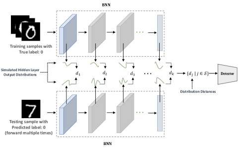
Figure 1: Framework of BATer. $k$ is the total number of hidden layers. $d_{j}$ represents the distribution distance measured from $j$-th hidden layer. $\mathcal{S}$ is the index set of selected hidden layers.

Despite many algorithms have been proposed for adversarial detection, most of them are deterministic, which means they can only use the information from one single forward pass to detect adversarial examples. This makes it easier for an attacker to break those models, especially when the attacker knows the neural network architecture and weights. In this paper, we propose a novel algorithm to detect adversarial examples based on randomized neural networks. Intuitively, incorporating randomness in neural networks can improve the smoothness of predictors, thus enabling stronger robustness guarantees (see randomized based defense methods in [24, 44, 11]). Further, instead of observing only one hidden feature for each layer, a randomized network can lead to a distribution of hidden features, making it easier for detecting an out-of-manifold example.

Contribution and Novelty

We propose a detection method based on Bayesian neural network (BNN), leveraging the randomness of BNN to improve detection performance (see framework in Figure 1). BNN and some other random components have been used to improve robust classification accuracy [24, 44, 25, 47, 11, 4], but they were not used to improve adversarial detection performance. The proposed method BATer is motivated by the following observations: 1) the hidden layer output generated from adversarial examples demonstrates different characteristics from that generated from natural data and this phenomenon is more obvious in BNN than deterministic deep neural networks; 2) randomness of BNN makes it easier to simulate the characteristics of hidden layer output. Training BNN is not very time-consuming as it only doubles the number of parameters of deep neural network with the same structure. However, BNN can achieve comparable classification accuracy and improve the smoothness of the classifier. A theoretical analysis is provided to show the advantage of BNN over DNN in adversarial detection.

In numerical experiments, our method achieves better performance in detecting adversarial examples generated from popular attack methods on MNIST, CIFAR10 and ImageNet-Sub among state-of-the-art detection methods. Ablation experiments show that BNN performs better than deterministic neural networks under the same detection scheme. Besides, customized white-box attacks are developed to break the proposed detection method and the results show that the proposed method can achieve reasonable performance under both customized strong white-box attack and high confidence attack.

Notation

In this paper, all the vectors are denoted as bold symbols. The input to the classifier is represented by ${\boldsymbol{x}}$ and the label associated with the input is represented by $y$. Thus, one observation is a pair $({\boldsymbol{x}},y)$. The classifier is denoted as $f(\cdot)$ and $f({\boldsymbol{x}})$ represents the output vector of the classifier. $f({\boldsymbol{x}})_{i}$ is the score of predicting ${\boldsymbol{x}}$ with label $i$. The prediction of the classifier is denoted as $c({\boldsymbol{x}})=\operatornamewithlimits{argmax}\limits_{i}f({\boldsymbol{x}})_{i}$; that is, the predicted label is the one with the highest prediction score. We use the $\ell_{\infty}$ and $\ell_{2}$ distortion metrics to measure similarity and report the $\ell_{\infty}$ distance in the normalized $[0,1]$ space (e.g., a distortion of $0.031$ corresponds to $8/256$), and the $\ell_{2}$ distance as the total root-mean-square distortion normalized by the total number of pixels.

2 Related Work

Adversarial attack

Multiple attack methods have been introduced for crafting adversarial examples to attack deep neural networks [48, 1, 5, 6, 30]. Depending on the information available to the adversary, attack methods can be divided into white-box attacks and black-box attacks. Under white-box setting, the adversary is allowed to analytically compute the model’s gradients/parameters, and has full access to the model architecture. Most white-box attacks generate adversarial examples based on the gradient of loss function with respect to the input [31, 8, 27, 6]. Among them FGSM, C$\&$W and PGD attacks have been widely used to test the robustness of machine learning models. In reality, the detailed model information, such as the gradient, may not be available to the attackers. Some attack methods are more agnostic and only rely on the predicted labels or scores [9, 3, 16, 10, 45]. [9] proposed a method to estimate the gradient based on the score information and craft adversarial examples with the estimated gradient. [3, 16, 10, 45, 7] introduced methods that also only rely on the final decision of the model.

Adversarial defense

To defend against adversarial examples, many studies have been done to improve the robustness of deep neural networks, including adversarial training [27, 20, 42, 49], generative models [36, 28, 23, 17] and verifiable defense [43]. The authors of [1] showed that many defense methods [12, 26, 36, 38, 44] can be circumvented by strong attacks except Madry’s adversarial training [27]. Since then adversarial training-based algorithms became state-of-the-art methods in defending against adversarial examples. However, adversarial training is computationally expensive and time-consuming due to the cost of generating adversarial examples on-the-fly, thus adversarial defense is still an open problem to solve.

Adversarial detection

Another popular line of research focuses on screening out adversarial examples. A straightforward way towards adversarial example detection is to build a simple binary classifier separating the adversarial apart from the clean data based on the characteristics of adversarial examples [14, 13, 22]. In [13], the author proposed to perform density estimation on the training data in the feature space of the last hidden layer to help detect adversarial examples (KD). The authors of [26] observed Local Intrinsic Dimension (LID) of hidden-layer outputs differ between the original and adversarial examples, and leveraged this characteristics to detect adversarial examples. In [22], the authors generated the class conditional Gaussian distributions with respect to lower-level and upper-level features of the deep neural network under Gaussian discriminant analysis, which result in a confidence score based on the Mahalanobis distance (MAHA), followed by a logistic regression model on the confidence scores to detect adversarial examples. In [46], the author studied the feature attributions of adversarial examples and proposed a detection method (ML-LOO) based on feature attribution scores. The author of [35] showed that adversarial examples exist in cone-like regions in very specific directions from their corresponding natural inputs and proposed a new test statistic to detect adversarial examples with the findings (ODD). Recently, a joint statistical testing pooling information from multiple layers is proposed in [33] to detect adversarial examples (ReBeL). Through vast experiments, we show that our method achieves comparable or superior performance than these detection methods across various attacks.

Bayesian neural network

The idea of BNN is illustrated in Figure 2. In [2], the author introduced an efficient algorithm to learn parameters of BNN. Given the observable random variables $({\boldsymbol{x}},y)$, BNN aims to estimate the distributions of hidden variables ${\boldsymbol{w}}$, instead of estimating the maximum likelihood value ${\boldsymbol{w}}_{\mathrm{MLE}}$ for the weights. Since in Bayesian perspective, each parameter is now a random variable measuring the uncertainty of the estimation, the model can potentially extract more information to support a better prediction (in terms of precision, robustness, etc.).

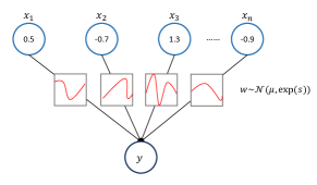
Figure 2: Illustration of Bayesian Neural Network.

Given the input ${\boldsymbol{x}}$ and label $y$, a BNN aims to estimate the posterior over the weights $p({\boldsymbol{w}}|{\boldsymbol{x}},y)$ given the prior $p({\boldsymbol{w}})$. The true posterior can be approximated by a parametric distribution $q_{\boldsymbol{\theta}}({\boldsymbol{w}})$, where the unknown parameter $\boldsymbol{\theta}$ is estimated by minimizing the KL divergence

$$\mathsf{KL}\big{(}q_{\boldsymbol{\theta}}({\boldsymbol{w}})\ \|\ p({\boldsymbol{w}}|{\boldsymbol{x}},y)\big{)}$$ (1)

over $\boldsymbol{\theta}$. For simplicity, $q_{\boldsymbol{\theta}}$ is often assumed to be a fully factorized Gaussian distribution:

$$q_{\boldsymbol{\theta}}({\boldsymbol{w}})=\prod_{i=1}^{d}q_{\boldsymbol{\theta}_{i}}({\boldsymbol{w}}_{i}),\text{ and }q_{\boldsymbol{\theta}_{i}}({\boldsymbol{w}}_{i})=\mathcal{N}({\boldsymbol{w}}_{i};\boldsymbol{\mu}_{i},\exp({\boldsymbol{s}}_{i})^{2}),$$ (2)

where ${\boldsymbol{\mu}}$ and ${\boldsymbol{s}}$ are parameters of the Gaussian distributions of weight. The objective function for training BNN is reformulated from expression (1) and is shown in expression (3), which is a sum of a data-dependent part and a regularization part:

$$\mathop{\arg\max}_{{\boldsymbol{\mu}},{\boldsymbol{s}}}\Big{\{}\sum_{({\boldsymbol{x}}_{i},y_{i})\in\boldsymbol{D}}\mathbb{E}_{{\boldsymbol{w}}\sim q_{{\boldsymbol{\mu}},{\boldsymbol{s}}}}\log p(y_{i}|{\boldsymbol{x}}_{i},{\boldsymbol{w}})-\mathsf{KL}\big{(}q_{{\boldsymbol{\mu}},{\boldsymbol{s}}}({\boldsymbol{w}})~{}\|~{}p({\boldsymbol{w}})\big{)}\Big{\}},$$ (3)

where $\boldsymbol{D}$ represents the data distribution. In the first term of objective (3), probability of $y_{i}$ given ${\boldsymbol{x}}_{i}$ and weights is the output of the model. This part represents the classification loss. The second term of objective (3) is trying to minimize the divergence between the prior and the parametric distribution, which can be viewed as regularization [2]. The author of [4] showed that the posterior average of the gradients of BNN makes it more robust than DNN against gradient-based adversarial attacks. Though the idea of using BNN to improve robustness against adversarial examples is not new [25, 47], the previous works did not use BNN to detect adversarial examples. In [25, 47], BNN was combined with adversarial training [27] to improve robust classification accuracy.

3 Proposed Method

We first discuss the motivation of the proposed method: 1) the distributions of the hidden layer neurons of DNN can be different for adversarial examples compared with natural examples; 2) this dispersion is more obvious in BNN than DNN; 3) it is easier to simulate hidden layer output distribution with random components. Then we introduce the specific metric used to measure this distributional difference and extend the detection method to multiple layers for making it more resistant to adversarial attacks.

3.1 Distributional difference of hidden layer outputs

Given input ${\boldsymbol{x}}$ and a classifier $f(\cdot)$, the prediction of the classifier is denoted as $c({\boldsymbol{x}})=\operatornamewithlimits{argmax}\limits_{i}f({\boldsymbol{x}})_{i}$; that is, the predicted label is the one with the highest prediction score. The adversary aims to perturb the original input to change the predicted label:

$$c({\boldsymbol{x}})\neq\operatornamewithlimits{argmax}\limits_{i}f({\boldsymbol{x}}+{\boldsymbol{\delta}})_{i},$$

where ${\boldsymbol{\delta}}$ denotes the perturbation added to the original input. The attacker aims to find a small ${\boldsymbol{\delta}}$ (usually lies within a small $\ell_{p}$ norm ball) to successfully change the prediction of the model. Thus, given the same predicted label, there could be distributional difference of hidden layer outputs between adversarial examples and natural data. For example, adversarial examples misclassified as airplanes could have hidden layer output distributions different from those of natural airplane images. Here, we define a hidden layer output distribution in DNN as the empirical distribution of all the neuron values of that layer. While in BNN, it is a real distribution as the weights of BNN are stochastic. The proposed method is motivated by the observation that the distribution of hidden layer outputs will be different under adversarial perturbations (e.g., Figure 3).

Why BNN not DNN?

Such pattern can be observed in both DNN and BNN. However, the distributional difference is more obvious in BNN than neural network without random component (see Figure 3). Therefore, more information can be extracted from BNN than general neural networks. Furthermore, random components of BNN make it easier to simulate the hidden layer output distributions. Our experimental results also show that the proposed detection method works better with BNN than with general neural networks on multiple datasets (see Section 4.2 for more details).

Figure 3 shows the hidden layer output distributions of layer $23$, layer $33$ and layer $43$ in DNN and BNN. Blue and cyan (train and test) curves represent distributions of the natural automobile images in CIFAR10. Red curves represent the distributions of adversarial examples mis-classified as automobile. The adversarial examples are generated by PGD [27] with $\ell_{\infty}$ norm. The DNN and BNN trained on CIFAR10 use the architecture of VGG16 [37] except that the weights in BNN follow Gaussian distributions. Hidden layer output distributions of train, test and adversarial examples are shown in blue, cyan and red. See details of attack parameters and network architectures in Appendix.

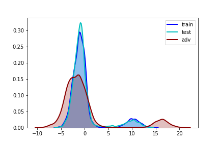
(a) BNN: Layer 23

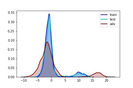
(b) BNN: Layer 33

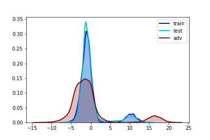
(c) BNN: Layer 43

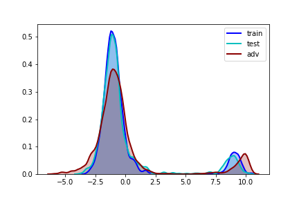
(d) DNN: Layer 23

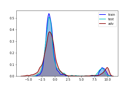
(e) DNN: Layer 33

(f) DNN: Layer 43

Figure 3: Hidden layer output distributions of BNN (VGG16 based structure) on automobile class of CIFAR10. train: Hidden layer output distributions of training examples from automobile class. test: Hidden layer output distributions of test examples from automobile class. adv: Hidden layer output distributions of adversarial examples predicted as automobile. The adversarial examples are generated by PGD [27].

We can see that for all three hidden layers, the distributional differences are more obvious in BNN than DNN. In BNN, the hidden layer output distributions of the natural images (train or test) are clearly different from those of adversarial examples (adv), while the pattern is not obvious in DNN. Even though hidden layer output distributions of only three layers are shown here, similar patterns are observed in some other layers in BNN. This phenomenon is not a special case with PGD adversarial examples on CIFAR10. Such characteristics are also found in adversarial examples generated by different attack methods on other datasets.

Figure 3 empirically shows the intuition behind the proposed framework. Theoretical analysis shows that randomness can help enlarge the distributional differences between natural and adversarial hidden layer outputs.

Proposition 1

Let $f({\boldsymbol{x}},{\boldsymbol{w}})$ be a model with ${\boldsymbol{x}}\sim\boldsymbol{D}_{\boldsymbol{x}}$ and ${\boldsymbol{w}}\sim\boldsymbol{D}_{\boldsymbol{w}}$, where $\boldsymbol{D}_{\boldsymbol{w}}$ is any distribution that satisfies ${\boldsymbol{w}}$ is symmetric about ${\boldsymbol{w}}_{0}=\mathbb{E}[{\boldsymbol{w}}]$, such as $\mathcal{N}({\boldsymbol{w}}_{0},\boldsymbol{I})$. If $\nabla_{\boldsymbol{x}}f({\boldsymbol{x}},{\boldsymbol{w}})$ can be approximated by the first order Taylor expansion at ${\boldsymbol{w}}_{0}$, we have

$$\mathcal{D}(f({\boldsymbol{x}}+{\boldsymbol{\delta}},{\boldsymbol{w}}),f({\boldsymbol{x}},{\boldsymbol{w}}))\geq\mathcal{D}(f({\boldsymbol{x}}+{\boldsymbol{\delta}},{\boldsymbol{w}}_{0}),f({\boldsymbol{x}},{\boldsymbol{w}}_{0})),$$ (4)

where ${\boldsymbol{\delta}}$ represents adversarial perturbation and $\mathcal{D}$ represents a translation-invariant distance measuring distribution dispersion (See proof of the inequality in Appendix).

The inequality shows that randomness involved in parameters will enlarge the distributional differences between natural and adversarial outputs. Therefore, we can leverage the distributional differences of multiple layers to detect adversarial examples.

3.2 Detect adversarial examples by distribution distance

We propose to measure the dispersion between hidden layer output distributions of adversarial examples and natural inputs and use this characteristic to detect adversarial examples. In particular, given an input ${\boldsymbol{x}}$ and its predicted label $c$, we measure the distribution distance between the hidden layer output distribution of ${\boldsymbol{x}}$ and the corresponding hidden layer output distribution of training samples from class $c$:

$$d_{j}({\boldsymbol{x}})=\mathcal{D}\left(h_{j}({\boldsymbol{x}}),h_{j}(\{{\boldsymbol{x}}^{c}_{i}\}_{i=1}^{n_{c}})\right),$$ (5)

where $h_{j}({\boldsymbol{x}})$ represents the hidden layer output distribution of the $j$-th layer based on testing sample ${\boldsymbol{x}}$, $h_{j}(\{{\boldsymbol{x}}^{c}_{i}\}_{i=1}^{n_{c}})$ represents the hidden layer output distribution of the $j$-th layer based on training samples from class $c$, $n_{c}$ is the number of training samples in class $c$, and $\mathcal{D}$ can be arbitrary divergence. In this paper, we estimate the divergence with 1-Wasserstein distance. However, other divergence measures can also be used, such as Kullback–Leibler divergence.

The hidden layer output distribution of training samples of each class can be easily simulated since there are multiple samples in each class. However, given predicted label, simulating the hidden layer output distribution of a testing sample is not easy. For general deep neural network without random components, the hidden layer output is deterministic, thus the simulation result depends on only a single forward pass. However, for BNN, the hidden layer output is stochastic, thus we can simulate the distribution with multiple passes of the input. To pool the information from different levels, the dispersion is measured at multiple hidden layers to generate a set of dispersion scores $\{d_{j}|j\in\mathcal{S}\}$, where $\mathcal{S}$ is the index set of selected hidden layers.

It is expected that natural inputs will have small dispersion scores while adversarial examples will have relatively large dispersion scores. A binary classifier is trained on the dispersion scores to detect adversarial examples. In the paper, we fit binomial logistic regression model to do the binary classification. Details of the method is included in Algorithm 1.

Algorithm 1 BATer

1:Input: Input ${\boldsymbol{x}}$, pre-trained BNN $f(\cdot)$, pre-trained binary classifier $g(\cdot)$, number of passes to simulate hidden layer output distribution $B$, indices of hidden layers selected for detection $\mathcal{S}$ and divergence $\mathcal{D}$.

2:Note: The output of the procedure is a binary indicator $z$, with $z=1$ indicating adversarial example and $z=0$ indicating natural input

3:procedure BayesianDetection(${\boldsymbol{x}},f,g,B,\mathcal{S},\mathcal{D}$)

4:     $c=\operatornamewithlimits{argmax}\limits_{i}f({\boldsymbol{x}})_{i}$

5:     for $j\in\mathcal{S}$ do

6:         Feed ${\boldsymbol{x}}$ into $f(\cdot)$ $B$ times to simulate $h_{j}({\boldsymbol{x}})$

7:         $d_{j}=\mathcal{D}(h_{j}({\boldsymbol{x}}),h_{j}^{c})$ $\triangleright$ $h_{j}^{c}$ is the $j$-th layer output distribution of class $c$      

8:     $z=g(d_{1},d_{2},...,d_{k})$

9:     Return: $z$

3.3 Implementation Details

Layer Selection

For adversarial examples generated with different attacks on different datasets, the pattern of distributional differences can be different. For example, adversarial examples generated by PGD on CIFAR10 show larger distributional dispersion in deeper layers (layers closer to final layer). However, such characteristic does not appear in adversarial examples generated by C$\&$W on CIFAR10. Instead, the distributional dispersion is more obvious in some front layers (layers closer to the input layer). Therefore, we develop an automate hidden layer selection scheme to find the layers with largest deviation between natural data and adversarial examples. Cross-validation is performed to do layer selection by fitting binary classifier (logistic regression) with a single layer’s dispersion score. Layers with top-ranked performance measured by AUC (area under the receiver operating characteristic curve) scores are selected, and information from those layers are pooled for ultimate detection (See details of selected layers in Appendix).

Distance Calculation

To measure the dispersion between hidden layer output distributions of natural and adversarial samples, we treat the output of a hidden layer as a realization of a one dimensional random variable. The dispersion between two distributions is estimated by 1-Wasserstein distance between their empirical distributions. In BNN, the empirical distribution of a test sample can be simulated by multiple forward passes. Whereas, in DNN, a single forward pass is done to simulate the empirical distribution as the output is deterministic. Training samples from the same class can be used to simulate empirical hidden layer output distributions of natural data of that class. Given a testing sample and its predicted label, calculating the dispersion score with all training samples in the predicted class is expensive, so we sample some natural images in the predicted class as representatives to speed up the process.

Dimension Reduction

To further improve computational efficiency, we apply dimension reduction on the hidden layer output. PCA (principal component analysis) is done with the hidden layer output of training samples to do dimension reduction before testing stage. At testing stage, hidden layer output is projected to lower dimension before calculating dispersion scores, which speeds up the dispersion score calculation with high-dimensional output.

4 Experimental Results

We evaluated BATer on the following well-known image classification datasets:

• MNIST [21]: handwritten digit dataset, which consists of $60,000$ training images and $10,000$ testing images. These are $28\times 28$ black and white images in ten different classes.

• CIFAR10 [19]: natural image dataset, which contains $50,000$ training images and $10,000$ testing images in ten different classes. These are low resolution $32\times 32$ color images.

• Imagenet-sub [29]: natural image dataset, which contains $158,617$ training images and $6,858$ testing images in $143$ different classes with resolution of $64\times 64$ pixels.

The training sets provided by the datasets are used to train BNN and DNN. The BNN and DNN architectures are the same except that the weights of BNN follow Gaussian distributions. The test sets are split into $20\%$ in training folds and $80\%$ in test folds. The detection models (binary classifiers) of KD, LID and BATer are trained on the training folds and the test folds are used to evaluate the performances of different detection methods. Foolbox [34] is used to generate adversarial examples with the following attack methods: FGSM [15] with $\ell_{\infty}$ norm, PGD [27] with $\ell_{\infty}$ norm and C$\&$W [5] with $\ell_{2}$ norm. Since BNN is stochastic, original PGD and C$\&$W attacks without considering randomness are not strong enough against it. For fair comparison, we update PGD and C$\&$W with stochastic optimization methods (multiple forward passes are used to estimate gradient not just one pass). Experiments in Section 4.1-4.2 and high confidence attack experiments in Section 4.3 are done in gray-box setting, in which we assume the adversary has access to the classifier model but does not know the detector. A customized attack is proposed in Section 4.3 to attack BATer in white-box setting, in which we assume the adversary has access to both classifier and detector. Details on parameters, neural network architectures, implementation and code are provided in Appendix.

4.1 Comparison with State-of-the-art Methods

We compare the performance of BATer with the following state-of-the-art detection methods for adversarial detection: 1) Kernel Density Detection (KD) [13], 2) Local intrinsic dimensionality detection (LID) [26], 3) Odds are odd detection (ODD) [35], 4) Reading Between the Layers (ReBeL) [33]. In [33], ReBeL outperforms deep mahalanobis detection [22] and trust score [18], so we do not include the performances of the two here. Details of implementation and parameters can be found in Appendix.

Table 1: Performance of detection methods against adversarial attacks.

Data	Metric	C$\&$W					FGSM					PGD
		KD	LID	ODD	ReBeL	BATer	KD	LID	ODD	ReBeL	BATer	KD	LID	ODD	ReBeL	BATer
CIFAR10	AUC	0.945	0.947	0.955	0.968	0.980	0.873	0.957	0.968	0.990	0.995	0.791	0.777	0.963	0.962	0.971
	TPR(FPR@0.01)	0.068	0.220	0.591	0.309	0.606	0.136	0.385	0.224	0.698	0.878	0.018	0.093	0.059	0.191	0.813
	TPR(FPR@0.05)	0.464	0.668	0.839	0.726	0.881	0.401	0.753	0.709	0.974	0.991	0.148	0.317	0.819	0.789	0.881
	TPR(FPR@0.10)	0.911	0.856	0.901	0.954	0.965	0.572	0.875	1.000	1.000	0.998	0.285	0.448	0.999	0.999	0.917
MNIST	AUC	0.932	0.785	0.968	0.980	0.999	0.933	0.888	0.952	0.992	0.999	0.801	0.861	0.967	0.975	0.989
	TPR(FPR@0.01)	0.196	0.079	0.212	0.630	0.974	0.421	0.152	0.898	0.885	0.972	0.062	0.170	0.607	0.382	0.733
	TPR(FPR@0.05)	0.616	0.263	0.911	0.900	0.997	0.692	0.503	0.908	0.990	0.998	0.275	0.396	0.934	0.851	0.957
	TPR(FPR@0.10)	0.818	0.397	1.000	0.972	1.000	0.796	0.678	0.917	1.000	1.000	0.429	0.552	0.945	0.956	0.999
Imagenet	AUC	0.811	0.905	0.886	0.834	0.941	0.914	0.983	0.844	0.842	0.989	0.989	0.991	0.777	0.824	0.976
	TPR(FPR@0.01)	0.193	0.401	0.185	0.035	0.146	0.460	0.772	0.042	0.045	0.569	0.930	0.829	0.010	0.028	0.729
-sub	TPR(FPR@0.05)	0.452	0.653	0.398	0.167	0.538	0.727	0.952	0.188	0.197	0.989	0.966	0.961	0.054	0.139	0.904
	TPR(FPR@0.10)	0.584	0.754	0.566	0.312	0.815	0.822	0.987	0.364	0.358	1.000	0.979	0.984	0.121	0.280	0.947

We report area under the curve (AUC) of the ROC curve as the performance evaluation criterion as well as the true positive rates (TPR) by thresholding false positive rates (FPR) at 0.01, 0.05 and 0.1, as it is practical to keep mis-classified natural data at a low proportion. TPR represents the proportion of adversarial examples classified as adversarial, and FPR represents the proportion of natural data mis-classified as adversarial. Before calculating performance metrics, all the samples that can be classified correctly by the model are removed. The results are reported in Table 1 and ROC curves are shown in Figure 4. BATer shows superior or comparable performance over the other four detection methods across three datasets.

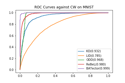
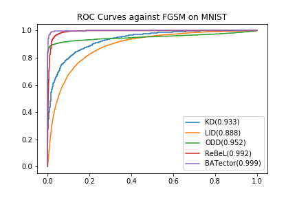
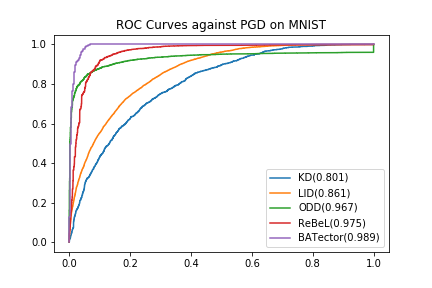
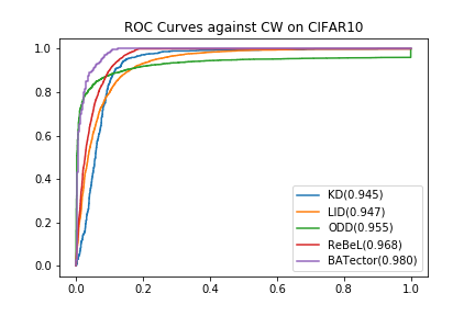
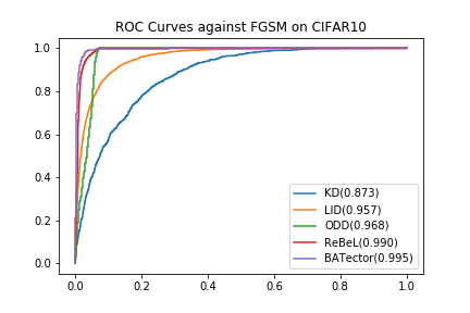
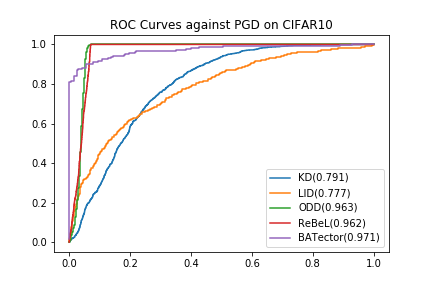
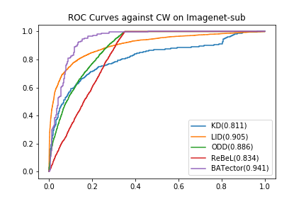
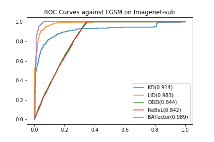
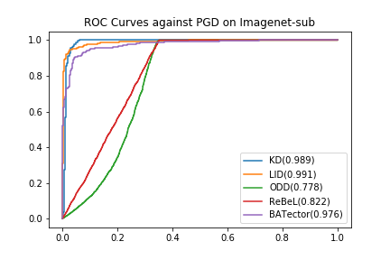
Figure 4: ROC Curves on MNIST, CIFAR10 and Imagenet-sub.

4.2 Ablation Study: BNN versus DNN

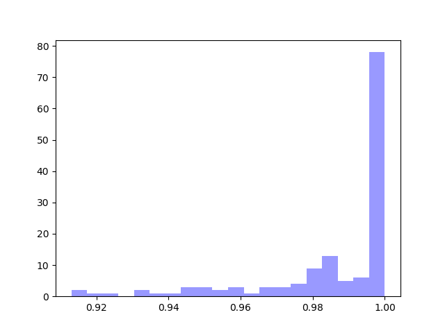
(a) AUC of BNN

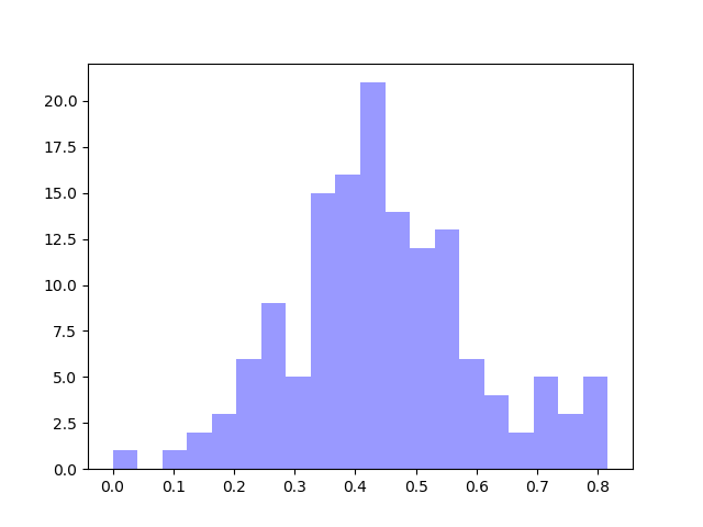
(b) AUC of DNN

Figure 5: AUC Histograms of BATer with different structures (BNN vs. DNN) on Imagenet-sub.

Table 2: AUC of BATer with different structures (BNN vs. DNN) on CIFAR10 and MNIST of different classes.

Class	CIFAR10		MNIST
	BNN	DNN	BNN	DNN
class1	0.978	0.489	0.929	0.901
class2	0.972	0.410	1.000	0.967
class3	0.973	0.501	0.993	0.892
class4	0.994	0.594	0.991	0.958
class5	0.955	0.477	1.000	0.883
class6	0.995	0.729	0.999	0.937
class7	0.976	0.584	0.989	0.878
class8	0.973	0.537	1.000	0.941
class9	0.915	0.493	0.959	0.874
lass10	0.949	0.567	0.982	0.917

In this section, we compare the performance of BATer using different structures (BNN versus DNN) against PGD across three datasets. The detection methods are the same (as described in Algorithm 1) and the differences are: 1) BATer with DNN uses pre-trained deep neural network of the same structure without random weights; 2) The number of passes is one as DNN does not produce different outputs with the same input. We report the class conditional AUC of the two different structures across three datasets.

The comparison results on CIFAR10 and MNIST are shown in Table 2 and the results on Imagenet-sub are shown in Figure 5. Since there $143$ classes in Imagenet-sub, it is not reasonable to show the results in a table. Instead, we show the AUC histograms of BATer with different structures in Figure 5. Comparing the AUC of applying BATer with BNN and DNN on CIFAR10 and MNIST, it is obvious that BNN structure demonstrates superior performances all the time. On Imagenet-sub, the AUC histogram of BATer with BNN ranges from $0.90$ to $1.00$ and is left-tailed, while the AUC histogram of BATer with DNN ranges from $0.10$ to $0.85$ and centers around $0.40$, so BNN structure clearly outperforms on Imagenet-sub.

4.3 High-confidence Attack and Customized Attack

Table 3: Performance of BATer against high-confidence C$\&$W and Restricted-PGD.

Data	Metric	C$\&$W (Confidence)			PGD	PGD_RES
		0	10	20
CIFAR10	AUC	0.980	0.999	0.995	0.971	0.893
	TPR(FPR@0.01)	0.606	0.998	0.939	0.813	0.002
	TPR(FPR@0.05)	0.881	1.000	0.995	0.881	0.321
	TPR(FPR@0.10)	0.965	1.000	0.995	0.917	0.606
MNIST	AUC	0.999	0.995	0.995	0.989	0.945
	TPR(FPR@0.01)	0.974	0.913	0.919	0.733	0.519
	TPR(FPR@0.05)	0.997	0.993	0.994	0.957	0.739
	TPR(FPR@0.10)	1.000	0.998	0.999	0.999	0.851
Imagenet	AUC	0.928	0.991	0.983	0.976	0. 915
	TPR(FPR@0.01)	0.146	0.896	0.642	0.729	0.221
-sub	TPR(FPR@0.05)	0.538	0.951	0.910	0.904	0.607
	TPR(FPR@0.10)	0.815	0.977	0.964	0.947	0.785

In [1], the authors pointed out that detection methods can fail when the confidence level of adversarial examples generated by C$\&$W attack increases. Therefore, we also test BATer against high-confidence adversarial examples across three datasets. Adversarial examples generated by C$\&$W with confidence $10$ and $20$ are used in the experiments. The performances of BATer are reported in Table 3. The results show that BATer performs well against high-confidence adversarial examples. Our analysis finds that the hidden layers selected to perform detection are different when defending against high-confidence adversarial examples. Increasing confidence level may change the characteristics of adversarial examples, but with proper layer selection, BATer can still detect them.

All the previous experiments are carried out in a gray-box setting, where we assume the adversary has access to the classifier model but does not know the details of the detector. The white-box setting assumes that the adversary has access to both classifier and detector. How to attack detection method under such setting is worth studying as it can reveal possible drawbacks of the method and promote future research direction. In this section, we develop a new white-box attack method customized for BATer, called Restricted-PGD. It would be hard to attack both classifier and detector of BATer as the detection process involves a distribution simulation process and Wasserstein distance estimation process, which are difficult to get gradient from. Therefore, directly modifying the objective function of a gradient-based attack method does not work here.

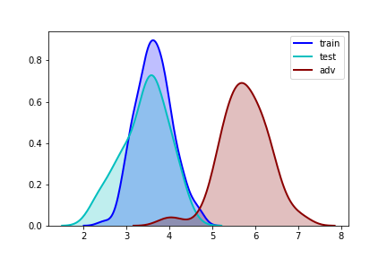
(a) BNN: Layer 23

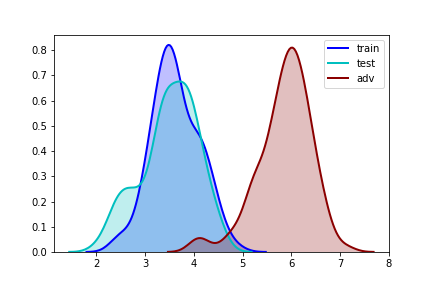
(b) BNN: Layer 33

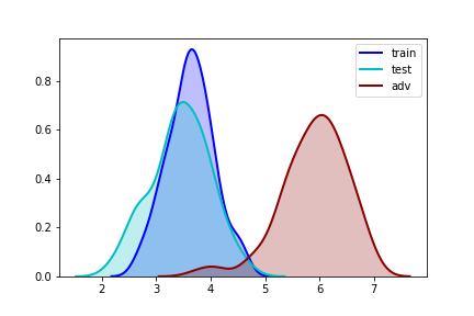
(c) BNN: Layer 43

Figure 6: Standard deviation distributions of hidden layer output of BNN on automobile class of CIFAR10. The adversarial examples are generated by PGD [27].

However, we carefully observe the hidden layer output distributions of natural data and adversarial examples and find an interesting pattern: the hidden layer output standard deviations of natural data and those of PGD adversarial examples are very different, which might be the key characteristics leveraged by the detection method to defend against PGD attack. In Figure 6, we show the standard deviation distributions of hidden layer output of natural data and those of PGD adversarial examples. It is obvious that hidden layer output standard deviations of adversarial examples have larger values than those of natural data. This characteristic will make the hidden layer output distributions of natural data and those of adversarial examples different.

Therefore, we propose an updated PGD attack to restrict the differences between predicted scores of different classes in the final layer, which will decrease the standard deviation of hidden layer output, especially for layers close to final layer. Given input ${\boldsymbol{x}}_{0}$ and its true label $y_{0}$, the objective function of Restricted-PGD is given by:

$$\operatorname*{argmin}\limits_{\|{\boldsymbol{x}}-{\boldsymbol{x}}_{0}\|_{\infty}\leq\epsilon}-L({\boldsymbol{x}},y_{0})+\lambda\sum_{i\neq j}\|f({\boldsymbol{x}})_{i}-f({\boldsymbol{x}})_{j}\|_{2},$$ (6)

where $L$ is the classification loss, $\epsilon$ is maximum perturbation and $\lambda$ controls the weight of the restriction part. One drawback of Restricted-PGD is that it may not be able to decrease the output standard deviations of layers in the front. For fair evaluation under white-box setting, only the last several layers are used by BATer to perform adversarial detection. Besides, the parameter $\lambda$ is also carefully tuned to make sure the attack is strong. The performances of BATer against Restricted-PGD across three datasets are shown in Table 3. Though the performances of BATer are affected by Restricted-PGD but are still good on MNIST and Imagenet-sub, and not bad on CIFAR10.

The hidden layer characteristics of adversarial examples generated by other attacks could be different from those of PGD. Therefore, the same trick may not work for FGSM and C$\&$W. Updated attack methods can be developed by carefully investigating the characteristics, and it could be a future research direction.

5 Conclusion

In this paper, we introduce a new framework to detect adversarial examples with Bayesian neural network, by capturing the distributional differences of multiple hidden layer outputs between the natural and adversarial examples. We show that our detection framework outperforms other state-of-the-art methods in detecting adversarial examples generated by various kinds of attacks. It also displays strong performance in detecting adversarial examples of high-confidence levels and adversarial examples generated by customized attack method.

Appendix A Datasets and DNN Architectures

One GPU (RTX 2080 Ti) is used in the experiment. The datasets used in the experiment do not contain personally identifiable information or offensive content. A summary of the datasets used, DNN architectures and test set performance of the corresponding DNNs are given in Table 4. For BNN, the structures used on the datasets are the same except that the weights of BNN are not deterministic but follow Gaussian distributions. See summary of BNN architectures and test set performances in Table 5.

Table 4: Datasets and DNN Architectures. Conv.: Convolutional layer, FC: Fully Connected layer, BN: Batch Normalization.

Dataset	Number of Classes	Test Accuracy	Architecture
MNIST [21]	10	99.20	2Conv. + 2FC layers
CIFAR10 [19]	10	93.34	VGG16 with BN [37]
Imagenet-Sub [29]	143	65.05	VGG16 with BN [37]

Table 5: Datasets and BNN Architectures. Conv.: Convolutional layer, FC: Fully Connected layer, BN: Batch Normalization. The structures of BNN are the same as DNN except that the weights of BNN are not deterministic but follow Gaussian distributions.

Dataset	Number of Classes	Test Accuracy	Architecture
MNIST [21]	10	98.81	2Conv. + 2FC layers
CIFAR10 [19]	10	92.32	VGG16 with BN [37]
Imagenet-Sub [29]	143	61.50	VGG16 with BN [37]

Appendix B Parameters of Attack Methods

Foolbox [34] is used to generate adversarial examples with C$\&$W, FGSM and PGD. Parameters used for the attack methods are listed below:

• C$\&$W [5] with $\ell_{2}$ norm: the confidence is set to $0$ for all three datasets except in high-confidence experiments, where the confidence values are discussed in section 4.3. The maximum number of iterations is set to $100$.

• FGSM [15] with $\ell_{\infty}$ norm: the maximum $\epsilon$ values of FGSM attack on MNIST, CIFAR10 and Imagenet-sub are set to $0.3$, $0.08$ and $0.08$ respectively.

• PGD [27] with $\ell_{\infty}$ norm: the $\epsilon$ values of PGD attack on MNIST, CIFAR10 and Imagenet-sub are set to $0.3$, $0.03$ and $0.02$ respectively. The number of iterations on MNIST, CIFAR10 and Imagenet-sub are set to $40$, $10$ and $10$ respectively. The step size of PGD attack on MNIST, CIFAR10 and Imagenet-sub are set to $0.1$, $0.01$ and $0.01$ respectively.

For Restricted-PGD attack, the parameter values are the same as PGD on three datasets. For high-confidence C$\&$W attack, the confidence is set to $10$ and $20$ on all three datasts and the maximum number of iterations is set to $100$.

Appendix C Layer Representations

Table 6: Selected layers and test statistics used in the experiments

Data	C$\&$W		FGSM		PGD
	Layers	Statistic	Layers	Statistic	Layers	Statistic
MNIST	[3, 5, 6]	min	[3, 5, 6]	min	[3, 5, 6]	min
CIFAR10	[4, 7]	min	[7]	mean	[39, 42, 43]	mean
Imagenet-Sub	[3, 7]	min	[7]	min	[39, 42, 43]	mean

A summary of the selected layers are given in Table 6. The distribution of each hidden layer in BNN is simulated with 4 forward passes of the inputs. We also list the summary statistics we use as a measure of average distance from the test sample to the natural image sets.

Appendix D Implementation of Detections

Implementation details of detection methods KD, LID, ODD, ReBeL and BATer are discussed in the following part:

• KD [13]: The Kernel Density Detection method is implemented by converting the author implementation into pytorch version. The author implementation is available at Github . The default parameter values are used for the experiments in this paper.

• LID [26]: The Local Intrinsic Dimension detection is implemented by using the code from Github . The numbers of neighbors used to calculate local intrinsic dimension are $10,20,30,40,50,60,70,80$ and $90$.

• ODD [35]: Odds are odd is implemented using the author original implementation with code available at Github . The default parameter values are used for the experiment in this paper.

• ReBeL [33]: Reading Between the Layers is implemented using the author original implementation with code available at Github . The test statistic is multinomial. The scoring method is p-value. Fisher method is used to combine the p-values from different layers. For other parameters, the default values are used.

• BATer: Code is available at Github .

Appendix E Theoretical Analysis

To show the advantage of BNN over DNN, there are two aspects. 1) BNN can better separate the distribution of natural hidden output and the distribution of natural hidden output. Figure 3 empirically shows it. 2) Randomness/Variance involved in the parameters can help enlarge the distributional differences between natural and adversarial outputs. The following analysis shows the second aspect.

E.1 Wasserstein Distance

In the paper, we estimate 1-Wasserstein distance between the distributions to detect adversarial examples. Here, we first show that BNN can enlarge distributional differences with this distance metric.

For a model $f({\boldsymbol{x}},{\boldsymbol{w}})$ with ${\boldsymbol{x}}\sim\boldsymbol{D}_{\boldsymbol{x}}$ and ${\boldsymbol{w}}\sim\boldsymbol{D}_{\boldsymbol{w}}$, where $\boldsymbol{D}_{\boldsymbol{w}}$ is any distribution that satisfies ${\boldsymbol{w}}$ is symmetric about ${\boldsymbol{w}}_{0}=\mathbb{E}[{\boldsymbol{w}}]$, such as $\mathcal{N}({\boldsymbol{w}}_{0},\boldsymbol{I})$. We want to show that

$$\mathcal{W}_{1}(f({\boldsymbol{x}}+{\boldsymbol{\delta}},{\boldsymbol{w}}),f({\boldsymbol{x}},{\boldsymbol{w}}))\geq\mathcal{W}_{1}(f({\boldsymbol{x}}+{\boldsymbol{\delta}},{\boldsymbol{w}}_{0}),f({\boldsymbol{x}},{\boldsymbol{w}}_{0})),$$

where $\mathcal{W}_{1}$ represents 1-Wasserstein distance, which measures distance between distribution of $f({\boldsymbol{x}}+{\boldsymbol{\delta}},{\boldsymbol{w}})$ and distribution of $f({\boldsymbol{x}},{\boldsymbol{w}})$.

As $f({\boldsymbol{x}}+{\boldsymbol{\delta}},{\boldsymbol{w}})\approx f({\boldsymbol{x}},{\boldsymbol{w}})+{\boldsymbol{\delta}}^{T}\nabla_{\boldsymbol{x}}f({\boldsymbol{x}},{\boldsymbol{w}})$, the distance can be approximated by

$$\mathcal{W}_{1}(f({\boldsymbol{x}}+{\boldsymbol{\delta}},{\boldsymbol{w}}_{0}),f({\boldsymbol{x}},{\boldsymbol{w}}_{0}))\approx{\boldsymbol{\delta}}\inf_{\pi}\int\|{\boldsymbol{\delta}}^{T}\nabla_{\boldsymbol{x}}f({\boldsymbol{x}},{\boldsymbol{w}}_{0})\|\pi({\boldsymbol{x}})$$

$$\mathcal{W}_{1}(f({\boldsymbol{x}}+{\boldsymbol{\delta}},{\boldsymbol{w}}),f({\boldsymbol{x}},{\boldsymbol{w}}))\approx\inf_{\pi\in\Gamma(\mathcal{D}_{\boldsymbol{x}},\mathcal{D}_{\boldsymbol{w}})}\int\|\delta^{T}\nabla_{\boldsymbol{x}}f({\boldsymbol{x}},{\boldsymbol{w}})\|\pi({\boldsymbol{x}},{\boldsymbol{w}})$$

If $\nabla_{\boldsymbol{x}}f({\boldsymbol{x}},{\boldsymbol{w}})$ can be further simplified with $\nabla_{\boldsymbol{x}}f({\boldsymbol{x}},{\boldsymbol{w}}_{0})+\nabla_{\boldsymbol{w}}\nabla_{\boldsymbol{x}}f({\boldsymbol{x}},{\boldsymbol{w}}_{0})({\boldsymbol{w}}-{\boldsymbol{w}}_{0})$,

$$\mathcal{W}_{1}(f({\boldsymbol{x}}+{\boldsymbol{\delta}},{\boldsymbol{w}}),f({\boldsymbol{x}},{\boldsymbol{w}})) ~{}\approx\inf_{\pi\in\Gamma(\mathcal{D}_{\boldsymbol{x}},\mathcal{D}_{\boldsymbol{w}})}\int\|{\boldsymbol{\delta}}^{T}\nabla_{\boldsymbol{x}}f({\boldsymbol{x}},{\boldsymbol{w}}_{0})+{\boldsymbol{\delta}}^{T}\nabla_{\boldsymbol{w}}\nabla_{\boldsymbol{x}}f({\boldsymbol{x}},{\boldsymbol{w}}_{0})({\boldsymbol{w}}-{\boldsymbol{w}}_{0})\|\pi({\boldsymbol{x}},{\boldsymbol{w}})$$

$$~{}=\inf_{\pi\in\Gamma(\mathcal{D}_{\boldsymbol{x}},\mathcal{D}_{\boldsymbol{w}})}\int\|{\boldsymbol{\delta}}^{T}\nabla_{\boldsymbol{x}}f({\boldsymbol{x}},{\boldsymbol{w}}_{0})+{\boldsymbol{\delta}}^{T}\nabla_{\boldsymbol{w}}\nabla_{\boldsymbol{x}}f({\boldsymbol{x}},{\boldsymbol{w}}_{0})({\boldsymbol{w}}_{0}-{\boldsymbol{w}})\|\pi({\boldsymbol{x}},{\boldsymbol{w}})$$

$$~{}\geq\inf_{\pi}\int\|{\boldsymbol{\delta}}^{T}\nabla_{\boldsymbol{x}}f({\boldsymbol{x}},{\boldsymbol{w}}_{0})\|\pi({\boldsymbol{x}})$$

$$~{}=\mathcal{W}_{1}(f({\boldsymbol{x}}+{\boldsymbol{\delta}},{\boldsymbol{w}}_{0}),f({\boldsymbol{x}},{\boldsymbol{w}}_{0}))$$

E.2 General Distance

The inequality can be extended to any translation-invariant distance. For a model $f({\boldsymbol{x}},{\boldsymbol{w}})$, where ${\boldsymbol{x}}\sim\boldsymbol{D}_{\boldsymbol{x}}$ and ${\boldsymbol{w}}\sim\boldsymbol{D}_{\boldsymbol{w}}$, then we want to show that

$$\mathcal{D}(f({\boldsymbol{x}}+{\boldsymbol{\delta}},{\boldsymbol{w}}),f({\boldsymbol{x}},{\boldsymbol{w}}))\geq\mathcal{D}(f({\boldsymbol{x}}+{\boldsymbol{\delta}},{\boldsymbol{w}}_{0}),f({\boldsymbol{x}},{\boldsymbol{w}}_{0})),$$ (7)

where ${\boldsymbol{\delta}}$ represents adversarial perturbation and $\mathcal{D}$ represents a translation-invariant distance measuring distribution dispersion.

As $f({\boldsymbol{x}}+{\boldsymbol{\delta}},{\boldsymbol{w}})\approx f({\boldsymbol{x}},{\boldsymbol{w}})+{\boldsymbol{\delta}}^{T}\nabla_{\boldsymbol{x}}f({\boldsymbol{x}},{\boldsymbol{w}})$ when $\|{\boldsymbol{\delta}}\|$ is small, the distance can be approximated by

$$\mathcal{D}(f({\boldsymbol{x}}+{\boldsymbol{\delta}},{\boldsymbol{w}}_{0}),f({\boldsymbol{x}},{\boldsymbol{w}}_{0}))\approx\mathcal{D}(f({\boldsymbol{x}},{\boldsymbol{w}}_{0})+{\boldsymbol{\delta}}^{T}\nabla_{\boldsymbol{x}}f({\boldsymbol{x}},{\boldsymbol{w}}_{0}),f({\boldsymbol{x}},{\boldsymbol{w}}_{0}))=\mathcal{D}({\boldsymbol{\delta}}^{T}\nabla_{\boldsymbol{x}}f({\boldsymbol{x}},{\boldsymbol{w}}_{0}),\boldsymbol{0})$$

$$\mathcal{D}(f({\boldsymbol{x}}+{\boldsymbol{\delta}},{\boldsymbol{w}}),f({\boldsymbol{x}},{\boldsymbol{w}}))\approx\mathcal{D}({\boldsymbol{\delta}}^{T}\nabla_{\boldsymbol{x}}f({\boldsymbol{x}},{\boldsymbol{w}}),\boldsymbol{0})$$

If $\nabla_{\boldsymbol{x}}f({\boldsymbol{x}},{\boldsymbol{w}})$ can be further simplified with $\nabla_{\boldsymbol{x}}f({\boldsymbol{x}},{\boldsymbol{w}}_{0})+\nabla_{\boldsymbol{w}}\nabla_{\boldsymbol{x}}f({\boldsymbol{x}},{\boldsymbol{w}}_{0})({\boldsymbol{w}}-{\boldsymbol{w}}_{0})$,

$$\mathcal{D}(f({\boldsymbol{x}}+{\boldsymbol{\delta}},{\boldsymbol{w}}),f({\boldsymbol{x}},{\boldsymbol{w}})) ~{}\approx\mathcal{D}({\boldsymbol{\delta}}^{T}\nabla_{\boldsymbol{x}}f({\boldsymbol{x}},{\boldsymbol{w}}_{0})+{\boldsymbol{\delta}}^{T}\nabla_{\boldsymbol{w}}\nabla_{\boldsymbol{x}}f({\boldsymbol{x}},{\boldsymbol{w}}_{0})({\boldsymbol{w}}-{\boldsymbol{w}}_{0}),\boldsymbol{0})$$

$$~{}=\mathcal{D}({\boldsymbol{\delta}}^{T}\nabla_{\boldsymbol{x}}f({\boldsymbol{x}},{\boldsymbol{w}}_{0}),{\boldsymbol{\delta}}^{T}\nabla_{\boldsymbol{w}}\nabla_{\boldsymbol{x}}f({\boldsymbol{x}},{\boldsymbol{w}}_{0})({\boldsymbol{w}}_{0}-{\boldsymbol{w}}))$$

$$~{}=\mathcal{D}(-{\boldsymbol{\delta}}^{T}\nabla_{\boldsymbol{x}}f({\boldsymbol{x}},{\boldsymbol{w}}_{0}),{\boldsymbol{\delta}}^{T}\nabla_{\boldsymbol{w}}\nabla_{\boldsymbol{x}}f({\boldsymbol{x}},{\boldsymbol{w}}_{0})({\boldsymbol{w}}_{0}-{\boldsymbol{w}}))$$

$$~{}\geq\frac{1}{2}\mathcal{D}({\boldsymbol{\delta}}^{T}\nabla_{\boldsymbol{x}}f({\boldsymbol{x}},{\boldsymbol{w}}_{0}),-{\boldsymbol{\delta}}^{T}\nabla_{\boldsymbol{x}}f({\boldsymbol{x}},{\boldsymbol{w}}_{0}))$$

$$~{}=\frac{1}{2}\mathcal{D}({\boldsymbol{\delta}}^{T}\nabla_{\boldsymbol{x}}f({\boldsymbol{x}},{\boldsymbol{w}}_{0}),\boldsymbol{0})$$

$$~{}\approx\mathcal{D}(f({\boldsymbol{x}}+{\boldsymbol{\delta}},{\boldsymbol{w}}_{0}),f({\boldsymbol{x}},{\boldsymbol{w}}_{0}))$$

where the third equality derives from translation-invariant of the metric and ${\boldsymbol{w}}_{0}-{\boldsymbol{w}}\sim{\boldsymbol{w}}-{\boldsymbol{w}}_{0}$ in distribution.

Appendix F Limitation and Impact

Security and reliability of machine learning systems are important. Adversarial examples cause concerns about the safety of machine learning systems in security sensitive areas, such as self-driving cars, flight control systems, healthcare systems and so on. The proposed method shows improvement of adversarial detection but it is not perfect. The performance of the method will drop when a customized attack is built to attack both the model and the detection method. The problem of adversarial example is far from solved. On the other hand, the research of adversarial examples shows the unreliable side of machine learning systems. Therefore, it may lead to a decrease of trust in such systems, and slow down the development and application of them.

References

- [1] A. Athalye, N. Carlini, and D. Wagner. Obfuscated gradients give a false sense of security: Circumventing defenses to adversarial examples. In International Conference on Machine Learning (ICML), 2018.
- [2] C. Blundell, J. Cornebise, K. Kavukcuoglu, and D. Wierstra. Weight uncertainty in neural network. In International Conference on Machine Learning, pages 1613–1622, 2015.
- [3] W. Brendel, J. Rauber, and M. Bethge. Decision-based adversarial attacks: Reliable attacks against black-box machine learning models. arXiv preprint arXiv:1712.04248, 2017.
- [4] G. Carbone, M. Wicker, L. Laurenti, A. Patane, L. Bortolussi, and G. Sanguinetti. Robustness of bayesian neural networks to gradient-based attacks. In H. Larochelle, M. Ranzato, R. Hadsell, M. F. Balcan, and H. Lin, editors, Advances in Neural Information Processing Systems, volume 33, pages 15602–15613. Curran Associates, Inc., 2020.
- [5] N. Carlini and D. Wagner. Adversarial examples are not easily detected: Bypassing ten detection methods. In Proceedings of the 10th ACM Workshop on Artificial Intelligence and Security, pages 3–14. ACM, 2017.
- [6] N. Carlini and D. Wagner. Towards evaluating the robustness of neural networks. In Security and Privacy (SP), 2017 IEEE Symposium on, pages 39–57. IEEE, 2017.
- [7] J. Chen, M. I. Jordan, and M. J. Wainwright. Hopskipjumpattack: A query-efficient decision-based attack. arXiv preprint arXiv:1904.02144, 2019.
- [8] P.-Y. Chen, Y. Sharma, H. Zhang, J. Yi, and C.-J. Hsieh. Ead: elastic-net attacks to deep neural networks via adversarial examples. In AAAI, 2018.
- [9] P.-Y. Chen, H. Zhang, Y. Sharma, J. Yi, and C.-J. Hsieh. Zoo: Zeroth order optimization based black-box attacks to deep neural networks without training substitute models. In Proceedings of the 10th ACM Workshop on Artificial Intelligence and Security, pages 15–26. ACM, 2017.
- [10] M. Cheng, S. Singh, P.-Y. Chen, S. Liu, and C.-J. Hsieh. Sign-opt: A query-efficient hard-label adversarial attack. arXiv preprint arXiv:1909.10773, 2019.
- [11] J. M. Cohen, E. Rosenfeld, and J. Z. Kolter. Certified adversarial robustness via randomized smoothing. arXiv preprint arXiv:1902.02918, 2019.
- [12] G. S. Dhillon, K. Azizzadenesheli, Z. C. Lipton, J. Bernstein, J. Kossaifi, A. Khanna, and A. Anandkumar. Stochastic activation pruning for robust adversarial defense. arXiv preprint arXiv:1803.01442, 2018.
- [13] R. Feinman, R. R. Curtin, S. Shintre, and A. B. Gardner. Detecting adversarial samples from artifacts. arXiv preprint arXiv:1703.00410, 2017.
- [14] Z. Gong, W. Wang, and W.-S. Ku. Adversarial and clean data are not twins. arXiv preprint arXiv:1704.04960, 2017.
- [15] I. Goodfellow, J. Shlens, and C. Szegedy. Explaining and harnessing adversarial examples. In International Conference on Learning Representations, 2015.
- [16] A. Ilyas, L. Engstrom, A. Athalye, and J. Lin. Black-box adversarial attacks with limited queries and information. arXiv preprint arXiv:1804.08598, 2018.
- [17] A. Jalal, A. Ilyas, C. Daskalakis, and A. G. Dimakis. The robust manifold defense: Adversarial training using generative models. arXiv preprint arXiv:1712.09196, 2017.
- [18] H. Jiang, B. Kim, M. Y. Guan, and M. R. Gupta. To trust or not to trust a classifier. In NeurIPS, pages 5546–5557, 2018.
- [19] A. Krizhevsky and G. Hinton. Learning multiple layers of features from tiny images. Technical report, Citeseer, 2009.
- [20] A. Kurakin, I. Goodfellow, and S. Bengio. Adversarial examples in the physical world. arXiv preprint arXiv:1607.02533, 2016.
- [21] Y. LeCun. The mnist database of handwritten digits. http://yann. lecun. com/exdb/mnist/, 1998.
- [22] K. Lee, K. Lee, H. Lee, and J. Shin. A simple unified framework for detecting out-of-distribution samples and adversarial attacks. In Advances in Neural Information Processing Systems, pages 7167–7177, 2018.
- [23] Y. Li, M. R. Min, W. Yu, C.-J. Hsieh, T. Lee, and E. Kruus. Optimal transport classifier: Defending against adversarial attacks by regularized deep embedding. arXiv preprint arXiv:1811.07950, 2020.
- [24] X. Liu, M. Cheng, H. Zhang, and C.-J. Hsieh. Towards robust neural networks via random self-ensemble. arXiv preprint arXiv:1712.00673, 2017.
- [25] X. Liu, Y. Li, C. Wu, and C.-J. Hsieh. Adv-BNN: Improved adversarial defense through robust bayesian neural network. In International Conference on Learning Representations, 2019.
- [26] X. Ma, B. Li, Y. Wang, S. M. Erfani, S. Wijewickrema, G. Schoenebeck, D. Song, M. E. Houle, and J. Bailey. Characterizing adversarial subspaces using local intrinsic dimensionality. arXiv preprint arXiv:1801.02613, 2018.
- [27] A. Madry, A. Makelov, L. Schmidt, D. Tsipras, and A. Vladu. Towards deep learning models resistant to adversarial attacks. arXiv preprint arXiv:1706.06083, 2017.
- [28] D. Meng and H. Chen. Magnet: a two-pronged defense against adversarial examples. In Proceedings of the 2017 ACM SIGSAC Conference on Computer and Communications Security, pages 135–147. ACM, 2017.
- [29] T. Miyato, T. Kataoka, M. Koyama, and Y. Yoshida. Spectral normalization for generative adversarial networks. arXiv preprint arXiv:1802.05957, 2018.
- [30] S.-M. Moosavi-Dezfooli, A. Fawzi, O. Fawzi, and P. Frossard. Universal adversarial perturbations. arXiv preprint, 2017.
- [31] S.-M. Moosavi-Dezfooli, A. Fawzi, and P. Frossard. Deepfool: a simple and accurate method to fool deep neural networks. In Proceedings of the IEEE Conference on Computer Vision and Pattern Recognition, pages 2574–2582, 2016.
- [32] T. Pang, C. Du, Y. Dong, and J. Zhu. Towards robust detection of adversarial examples. In Advances in Neural Information Processing Systems, pages 4584–4594, 2018.
- [33] J. Raghuram, V. Chandrasekaran, S. Jha, and S. Banerjee. Detecting anomalous inputs to dnn classifiers by joint statistical testing at the layers. arXiv preprint arXiv:2007.15147, 2020.
- [34] J. Rauber, W. Brendel, and M. Bethge. Foolbox: A python toolbox to benchmark the robustness of machine learning models. arXiv preprint arXiv:1707.04131, 2017.
- [35] K. Roth, Y. Kilcher, and T. Hofmann. The odds are odd: A statistical test for detecting adversarial examples. In International Conference on Machine Learning, pages 5498–5507. PMLR, 2019.
- [36] P. Samangouei, M. Kabkab, and R. Chellappa. Defense-gan: Protecting classifiers against adversarial attacks using generative models. arXiv preprint arXiv:1805.06605, 2018.
- [37] K. Simonyan and A. Zisserman. Very deep convolutional networks for large-scale image recognition. arXiv preprint arXiv:1409.1556, 2014.
- [38] Y. Song, T. Kim, S. Nowozin, S. Ermon, and N. Kushman. Pixeldefend: Leveraging generative models to understand and defend against adversarial examples. arXiv preprint arXiv:1710.10766, 2017.
- [39] C. Szegedy, W. Zaremba, I. Sutskever, J. Bruna, D. Erhan, I. Goodfellow, and R. Fergus. Intriguing properties of neural networks. arXiv preprint arXiv:1312.6199, 2013.
- [40] T. Tanay and L. Griffin. A boundary tilting persepective on the phenomenon of adversarial examples. arXiv preprint arXiv:1608.07690, 2016.
- [41] G. Tao, S. Ma, Y. Liu, and X. Zhang. Attacks meet interpretability: Attribute-steered detection of adversarial samples. In Advances in Neural Information Processing Systems, pages 7717–7728, 2018.
- [42] F. Tramèr, A. Kurakin, N. Papernot, I. Goodfellow, D. Boneh, and P. McDaniel. Ensemble adversarial training: Attacks and defenses. arXiv preprint arXiv:1705.07204, 2017.
- [43] E. Wong and Z. Kolter. Provable defenses against adversarial examples via the convex outer adversarial polytope. In International Conference on Machine Learning, pages 5286–5295. PMLR, 2018.
- [44] C. Xie, J. Wang, Z. Zhang, Z. Ren, and A. Yuille. Mitigating adversarial effects through randomization. arXiv preprint arXiv:1711.01991, 2017.
- [45] Z. Yan, Y. Guo, and C. Zhang. Subspace attack: Exploiting promising subspaces for query-efficient black-box attacks. arXiv preprint arXiv:1906.04392, 2019.
- [46] P. Yang, J. Chen, C.-J. Hsieh, J.-L. Wang, and M. Jordan. Ml-loo: Detecting adversarial examples with feature attribution. In Proceedings of the AAAI Conference on Artificial Intelligence, volume 34, pages 6639–6647, 2020.
- [47] N. Ye and Z. Zhu. Bayesian adversarial learning. In S. Bengio, H. Wallach, H. Larochelle, K. Grauman, N. Cesa-Bianchi, and R. Garnett, editors, Advances in Neural Information Processing Systems 31, pages 6892–6901. Curran Associates, Inc., 2018.
- [48] X. Yuan, P. He, Q. Zhu, and X. Li. Adversarial examples: Attacks and defenses for deep learning. IEEE Transactions on Neural Networks and Learning Systems, 2019.
- [49] H. Zhang, Y. Yu, J. Jiao, E. P. Xing, L. E. Ghaoui, and M. I. Jordan. Theoretically principled trade-off between robustness and accuracy. arXiv preprint arXiv:1901.08573, 2019.
- [50] Z. Zheng and P. Hong. Robust detection of adversarial attacks by modeling the intrinsic properties of deep neural networks. In Advances in Neural Information Processing Systems, pages 7913–7922, 2018.