On the Robustness of Domain Constraints

Abstract.

Machine learning is vulnerable to adversarial examples–inputs designed to cause models to perform poorly. However, it is unclear if adversarial examples represent realistic inputs in the modeled domains. Diverse domains such as networks and phishing have domain constraints–complex relationships between features that an adversary must satisfy for an attack to be realized (in addition to any adversary-specific goals). In this paper, we explore how domain constraints limit adversarial capabilities and how adversaries can adapt their strategies to create realistic (constraint-compliant) examples. In this, we develop techniques to learn domain constraints from data, and show how the learned constraints can be integrated into the adversarial crafting process. We evaluate the efficacy of our approach in network intrusion and phishing datasets and find: (1) up to $82\text{\,}\mathrm{\char 37\relax}$ of adversarial examples produced by state-of-the-art crafting algorithms violate domain constraints, (2) domain constraints are robust to adversarial examples; enforcing constraints yields an increase in model accuracy by up to $34\text{\,}\mathrm{\char 37\relax}$. We observe not only that adversaries must alter inputs to satisfy domain constraints, but that these constraints make the generation of valid adversarial examples far more challenging.

1. Introduction

Machine learning has demonstrated exceptional problem-solving capabilities; it has become the tool to learn, tune, and deploy for many important domains, including healthcare, finance, education, and security (esteva_guide_2019, ; heaton_deep_2016, ; popenici_exploring_2017, ; buczak_survey_2016, ). However, machine learning is not without its own limitations: countless works have demonstrated the fragility of models when in the presence of an adversary (goodfellow_explaining_2014, ; kurakin_adversarial_2016, ; papernot_limitations_2016, ; carlini_towards_2017, ; madry_towards_2017, ). Across a variety of threat models, research has shown how adversaries fully control model outputs, by classifying school buses as ostriches (szegedy_intriguing_2013, ), students as celebrities (sharif_accessorize_2016, ), or generating photos of synthetic, yet unsettlingly realistic, people (goodfellow_generative_2014, ).

This field of adversarial machine learning is rich with research into the exploitation of these models. While alarming to domains that have observed significant advancements as a result of machine learning (i.e., network intrusion detection, spam, malware, etc.), it is not clear yet whether these domains are as vulnerable as posited. This observation is rooted in the domain which exemplifies the end-to-end capability of deep learning: images. Influential works often use images as an empirical demonstration of their findings (goodfellow_explaining_2014, ; papernot_limitations_2016, ; carlini_towards_2017, ; madry_towards_2017, ; kurakin_adversarial_2016, ). This has an implicit assumption on the underlying threat models; adversaries can manipulate features arbitrarily and independently. In other words, adversaries are assumed to have full control over the feature space and, more importantly, all input manipulations are equally permissible in the domain under investigation. While often bound (exclusively) by some self-imposed $\ell_{\mathscr{p}}$-norm (canonically used as a surrogate for human perception), there are constructs, rules, and other forms of domain constraints that many domains contain which images do not.

Domain constraints describe relationships between features. For example, in network flow data, TCP flags can only be set for TCP flows in networks—having these flags for UDP would violate the semantics of the underlying phenomenon (network protocols). Constraints encode the maneuvers (i.e., perturbations) that are possible for an adversary when crafting adversarial examples. Yet, existing threat models broadly ignore this requirement, serving to generate examples that may or may not represent legitimate examples of the domain. Thus, any vigilant system could simply discard non-compliant samples because they are manifestly adversarial—they do not represent a sample that could benignly exist. Such detectable adversarial examples, thus, pose no risk.

We argue in this paper that to properly assess the practical vulnerability of machine learning in a domain, the constraints that characterize the domain must be learned, incorporated, and demonstrated in attacks. Naturally, some domains contain incredibly rigid structures (e.g., binaries or networks) that could offer robustness against adversaries (that is, an inability to craft realizable adversarial examples), which is one of the central questions we investigate in this paper. By learning domain constraints, those who use machine learning can build accurate threat models and thus, properly assess realistic attack vectors.

Learning what the constraints are in arbitrary domains is a non-trivial process; domains can contain multiple layers of complex abstractions, frustrating any manual constraint identification through expertise. Fortunately, there are data-driven approaches for learning and encoding useful representations of constraints from areas within formal logic. One such method comes from the seminal work of Leslie Valiant on PAC learning (probably approximately correct learning) (valiant_theory_1984, ). In this work, Valiant described a setting for learning boolean constraints (specifically, $k$-conjunctive normal form (CNF)) theories from data. Valiant’s constraint theory formulation and paired learning protocol provides a simple, yet exhaustive, mechanism for identifying constraints and, coincidentally, an elegant representation for integration into adversarial crafting algorithms.

In order to understand the robustness provided by domain constraints, we characterize the worst-case adversary. Specifically, the worst-case adversary is defined as one who is least constrained. Said formally, the number of possible observations rejected by a constraint theory is minimal. We describe the worst-case adversary by exploiting a theoretical property in our setting; a constraint theory is sound if the observations it certifies comply with the domain constraints. From this property, we show that sound constraint theories reduce to memorization of the training data, and how easing soundness yields generalization, with the worst-case adversary occurring under the most general (i.e., least constrained) constraint theory that can be learned.

In this paper, we explore adversarial examples with domain constraints by answering two fundamental questions: (1) How would adversaries launch attacks in constrained domains?, and (2) Are constrained domains robust against adversarial examples? We design our approach by leveraging frameworks within formal logic to learn constraints from data. Then, we modify an algorithm for constraint satisfaction, Davis-Putnam-Logemann-Loveland (DPLL), to project adversarial examples onto a constraint-compliant space. Finally, we introduce a new adversarial crafting algorithm, the Constrained Saliency Projection (CSP): a blend of two popular adversarial crafting algorithms that, by design, aids DPLL in projection. We evaluate the efficacy of our approach on network intrusion detection and phishing datasets. From our investigation, we argue that incorporating domain constraints into threat models is necessary to produce realistic adversarial examples, and more importantly, constrained domains are naturally more robust to adversarial examples than unconstrained domains (e.g., images).

We contribute the following:

1. We formalize domain constraints in machine learning.

2. We prove theoretical guarantees for learning domain constraints in our setting. We describe when and why constraint theories are sound and complete, demonstrating an inherent trade-off between generalization and soundness.

3. We satisfy domain constraints by projecting non-realizable adversarial examples onto the space of valid inputs. We also introduce the Constrained Saliency Projection (CSP).

4. We demonstrate the robustness produced by domain constraints against worst-case adversaries in two diverse datasets. We observe that enforcing domain constraints can improve the robustness of a model substantially; in one experiment constraint enforcement restored model accuracy by $34\text{\,}\mathrm{\char 37\relax}$.

2. Overview

In order to measure the robustness of constrained domains against adversarial examples, we must build a new set of techniques. We can envision this process in three parts: (1) learning the domain constraints, (2) crafting adversarial examples, and (3) projecting adversarial examples onto a constraint-compliant space. A visualization of this approach is described in Figure 1.

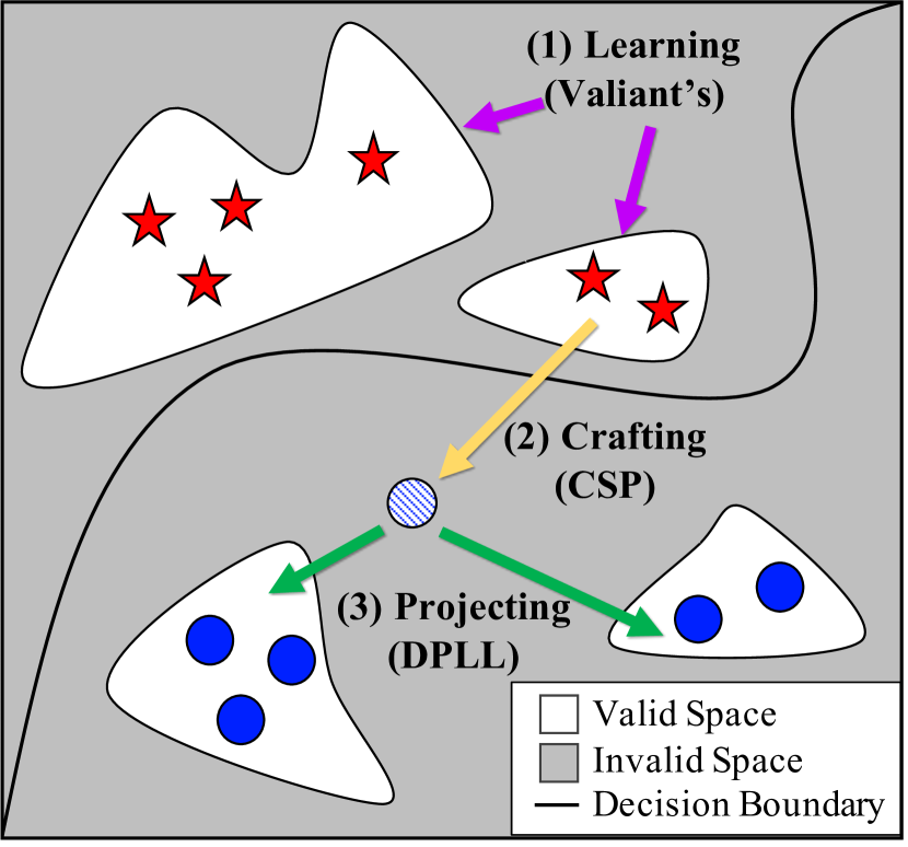
Figure 1. An Overview of Our Approach—Our approach consists of three steps: (1) learning the domain constraints, (2) crafting adversarial examples, and (3) projecting adversarial examples onto a constraint-compliant space.

Learning Constraints. In many domains, there are regions for which samples do not exist (e.g., UDP flows in the network domain do not have TCP flags). The structures and rules that define these regions may be complex and thus, we need a general approach to learn how domains are partitioned into valid and invalid regions. We leverage an algorithm from PAC learning, Valiant’s algorithm, to learn these domain constraints in Section 4.2.

Crafting Adversarial Examples. After domain constraints have been learned, our approach can leverage any adversarial crafting algorithm. While there are many (goodfellow_explaining_2014, ; papernot_limitations_2016, ; carlini_towards_2017, ; madry_towards_2017, ) attacks in literature, we focus on PGD in Section 4.4 as it is considered to be the state-of-the-art for first-order adversaries. We will also consider a constraint-specific approach in Section 4.6.

Projecting Adversarial Examples. With the learned domain constraints and a set of adversarial examples, we must now enforce the constraints on the crafted adversarial examples. We do this by projecting the adversarial examples onto the constraint-compliant space (defined within some budget, as to preserve the goals of the adversary). Specifically, we manipulate features in constraint-noncompliant adversarial examples until they either satisfy the domain constraints or exceed the allotted budget. We augment a seminal solver for constraint satisfaction, Davis-Putnam-Logeman-Loveland, to perform this projection in Section 4.5.

3. Background

3.1. Threat Model

Adversarial Goals. Adversaries can have a variety of objectives, from reducing model confidence to misclassifying a sample as a particular target. Here, we focus on the former, that is, given a victim model $f_{\theta}$ with parameters $\theta$, a sample $e$, label $y$, a self-imposed budget $\phi$ measured under some $\ell_{\mathscr{p}}$-norm, and a domain-dictated constraint theory $T$ (which is our contribution), an adversary aims to solve the following optimization objective:

—l— α∥α∥_p f_θ(e + α) ≠ y e + α∈B_ϕ(e) ∩ T

Conceptually, the adversary searches within some norm-ball $\mathcal{B}$ of radius $\phi$ around a sample $e$ for a “small” change $\alpha$ to apply to $e$ that yields the desirable model behavior (i.e., an adversarial example). In the context of computer security, this could translate to bypassing a network intrusion detection system.

“White-box” settings represent the strongest adversaries and characterize worst-case scenarios. Akin to insider threats, these adversaries have unfettered queries to the model, can observe its parameters, and can use its training data. From Equation 3.1, suppose $f_{\theta}$ describes the model of the defender, then white-box adversaries either have direct access to model parameters of $f_{\theta}$ or the training data used to learn $f_{\theta}$. Practically speaking, such adversaries can produce adversarial examples with the tightest $\ell_{\mathscr{p}}$-norm constraints (i.e., the smallest budgets). “Gray-” and “Black-box” threat models are two other popular threat models that remove the degree to which an adversary has access to model parameters or training data. These limited adversaries usually require unique techniques for attacks to be successful (papernot_transferability_2016, ; liu_delving_2016, ; tramer_space_2017, ).

In our work, we explore the efficacy of white-box adversaries when domain constraints are enforced. Specifically, the adversary seeks to minimize model accuracy (that is, the number of samples correctly classified over the total number of samples). Referring to Equation 3.1, the adversary computes samples classified as any class $\hat{y}\neq y$ (where $\hat{y}$ is the prediction). Under this objective, the adversary attempts to reduce the confidence an operator has in the predictions of a model.

3.2. Adversarial Machine Learning

We describe the two algorithms that serve as the basis for the algorithm used in our approach discussed later in Section 4.4.

Jacobian-based Saliency Map Approach (JSMA). The JSMA (papernot_limitations_2016, ) is an iterative approach leveraging saliency maps: a heuristic applied to the Jacobian matrix of the model. For our work, the insightful component of the JSMA is that it selects a single feature to perturb per iteration (i.e., it optimizes over $\ell_{0}$-norms). This is especially important for security-critical domains as other $\ell_{\mathscr{p}\neq{}0}$-norms are largely driven as surrogates for human perception, and do not apply to the studied domains.

Projected Gradient Descent (PGD). PGD, by Madry et al., is considered to be the state-of-the-art for first-order adversaries (madry_towards_2017, ). Similar to the Fast Gradient Sign Method (goodfellow_explaining_2014, ), PGD iteratively multiplies a step-size $\alpha$ by the sign of the gradient of the loss to perturb the sample. As PGD has been proposed as a “universal adversary (among first-order approaches),” (madry_towards_2017, ) we use it to evaluate the robustness of constraints against adversarial examples.

4. Approach

4.1. Preliminaries

We overview constraint learning and define the three algorithms we leverage for constraint learning, projection, and clustering.

Problem Statement. (raedt_learning_nodate, ) provided one formulation for framing constraint learning as a concept-learning problem. We restate the relevant parts of the formalization for our work. Namely, we are given a domain $X=(X_{1},\dots,X_{n})$, where $X_{i}\subseteq\mathbb{Z}$ (i.e., we have $n$ features where $X_{n}$ denotes the unique values feature $n$ can take), a space $C$ of possible constraints (represented as $k$-CNF Boolean formulae defined over $X$), and a set $E$ of collected observations. Our objective is to find a constraint theory $T$ ($T\subseteq C$) such that $T$ certifies all observations $e\in E$. We say $T$ certifies $e$ when all clauses $t\in T$ are satisfied by $e$. We say a clause $t$ is satisfied when at least one literal in $t$ is True (where the features in $e$ assign values to the literals in $t$). Conceptually, the collected observations $E$ encode the structures or rules of the domain (i.e., $T$), that we seek to learn.

Valiant’s Algorithm. Valiant’s algorithm (Algorithm 1) is a general, exhaustive, generate-and-test algorithm for constraint learning (valiant_theory_1984, ). The algorithm is initialized with a constraint theory $T$ of all possible constraints over $X$ (i.e., $T=C$). Then, for each observation $e\in E$, clauses that are not satisfied by $e$ are removed from $T$. The algorithm terminates when $E$ has been exhaustively processed. Valiant’s algorithm will converge to the correct solution, assuming $E$ sufficiently represents the domain and is free of noise. Moreover, Valiant’s algorithm does not require any negative examples (that is, known observations that violate domain constraints, which are absent from popular machine learning datasets), which some constraint learning approaches require (garg_ice_2014, ; zhu_data-driven_2018, ). Conceptually, $T$ initially describes the space of possible constraints and, after applying $T$ and the set, $E$, of collected observations to Valiant’s algorithm, $T$ will contain the set of constraints that are satisfied by all observations in $E$ (in other words, the intersection of satisfied constraints across the observations in $E$).

Input: observations $E$, boolean clauses $T$

Output: a conjunction of the remaining clauses $T$

1 for $e\in E$ do

2      for $c\in T$ do

3            remove $c$ from $T$ if $e\nvdash c$

4       end for

5      

6 end for

return $T$

Algorithm 1 Valiant’s Algorithm

Input: a domain $X$

Output: the space of possible constraints $C$

1

2$P\leftarrow\{\mathscr{P}{}(X_{i})\setminus\{\varnothing,X_{i}\}\mid X_{i}\in X\}$

3 $C\leftarrow\{P_{1}\times\dotsb\times P_{n}\}$, $P_{i}\in P$

4 $C\leftarrow$ RelaxToCNF(C)

5 return $C$

6

Algorithm 2 Generating the Space of Possible Constraints

To illustrate how Valiant’s algorithm operates, consider an example where a dataset contains samples with two binary features, $X_{1}=\{x_{1},\neg x_{1}\}$ and $X_{2}=\{x_{2},\neg x_{2}\}$. Then, $C$, the space of possible constraints is:

$$C=(x_{1}\lor x_{2})\land(x_{1}\lor\neg x_{2})\land(\neg x_{1}\lor x_{2})\land(\neg x_{1}\lor\neg x_{2})$$

If we initialize $T$ (our target constraint theory) to $C$, and suppose $E$ (our set of collected observations) consists of two observations $e_{1}=(\textsc{False},\textsc{False})$ and $e_{2}=(\textsc{True},\textsc{True})$, then Valiant’s algorithm first removes $(x_{1}\lor x_{2})$, and then removes $(\neg x_{1}\lor\neg x_{2})$ (as they are not satisfied by $e_{1}$ and $e_{2}$, respectively). Our final constraint theory $T$ is then $(x_{1}\lor\neg x_{2})\land(\neg x_{1}\lor x2)$. This example shows the thesis behind Valiant’s algorithm: only constraints that have support from all observations are permissible.

DPLL. For adversarial examples that do not comply with domain constraints, we use an algorithm from the constraint satisfaction community, Davis-Putnam-Logeman-Loveland (DPLL) (davis_computing_1960, ), to project adversarial examples onto the learned constraint theory returned by Valiant’s Algorithm. DPLL has some characteristics that make it ideal for our task, namely: (1) it accepts boolean formulae in CNF (which is the native form of the constraint theories learned by Valiant’s Algorithm), and (2) it is a backtracking-based search algorithm: DPLL iteratively builds candidate solutions for a given expression, which is a property we exploit, detailed later in Section 4.5. Further details about DPLL can be found in Appendix C.4

OPTICS. Later, we show how we model arbitrary data types as domain constraints. To support this generalization, we leverage a clustering algorithm, Ordering Points to Identify the Clustering Structure (OPTICS) (ankerst_optics_1999, ). OPTICS has two advantages over other clustering algorithms for our application, namely: (1) it scales to large sample sizes, and (2) it is not parameterized on specifying the number of clusters. The second property is particularly important as parameterizing the number of clusters assumes a priori knowledge of the constraints before learning them in the first place.

4.2. Learning Constraints

Recall our problem statement: given a domain $X$, we first generate the space $C$ of possible constraints, then, with a dataset $E$ of samples, we use Valiant’s algorithm to prune constraints that do not comply with samples in our dataset (i.e., $T\subseteq C$). Valiant’s algorithm is elegant for binary features and the fact that it produces “hard” boolean constraints makes it attractive for encoding rigorous structures of domains. However, novel applications of machine learning seldom use binary features exclusively; categorical and continuous features (e.g., packet rates or word counts) are used in nearly every modern application of machine learning.

To address this limitation, there are two modifications that must be made: (1) how the space of possible constraints is generated, and (2) how to determine if a particular sample is certified by a constraint theory. We discuss these two modifications below.

The Space of Possible Constraints. For boolean-only constraint theories, the space of possible constraints is on the order of $\mathcal{O}{}(2^{n})$, where $n$ is the number of features. To account for categorical features, we can further generalize this bound to $\mathcal{O}{}(2^{n\cdot i})$ by considering a one-hot encoding, where $i$ represents the largest cardinality of possible values among $n$ features. This guides us on not only how to generate the space of constraints, but also how to modify Valiant’s algorithm to accept a richer representation of constraints.

Our approach, shown in Algorithm 2, is as follows: first, given a domain $X$, we compute a pseudo-power set $P_{i}$ from the set $X_{i}$ of unique values for feature $i$. $P_{i}$ is a pseudo-power set as we remove the empty set (i.e., no value is valid for the feature) and $X_{i}$ (which would allow the constraint to be trivially satisfied by any sample). We then perform the Cartesian product over $P$, which returns the set of all possible combinations of constraints; this is the input to Valiant’s algorithm ($C$). At this stage, $C$ contains sets $P_{i}$ of sets $p_{i}$, and so, we transform this representation to CNF (RelaxToCNF) by adding disjunctions between each $p_{i}\in P_{i}$ and, finally adding conjunctions between each $P_{i}\in C$.

To adapt Valiant’s algorithm to perform on a set-based representation of constraints (i.e., boolean and categorical variables), we redefine the $\vdash$ operator (i.e., logical entailment); instead of evaluating whether or not a feature value causes a boolean assignment to be satisfied, we instead evaluate if it is a member of the set (i.e., $\nvdash$ now operates as $\notin$, set membership, in Algorithm 1).

Consider the following example: suppose two features, $X_{1}$ and $X_{2}$. Let $X_{1}$ be a boolean variable (encoded as $x_{1}\in\{0,1\}$) and let $X_{2}$ be a categorical variable that can take on one of three values (encoded as $x_{2}\in\{A,B,C\}$). With our approach above, the space of possible constraints is then:

$$\begin{split}C=(x_{1}\in\{0\}\lor x_{2}\in\{A\})&\land(x_{1}\in\{0\}\lor x_{2}\in\{B\})\\ &\cdots\\ \land(x_{1}\in\{1\}\lor x_{2}\in\{A,C\})&\land(x_{1}\in\{1\}\lor x_{2}\in\{B,C\})\end{split}$$

If we initialize our target constraint theory $T$ to $C$, and let $E$ (our training data) consists of four samples $e_{1}=(0,A)$, $e_{2}=(0,B)$, $e_{3}=(1,B)$, and $e_{4}=(1,C)$, then our objective is to guide Valiant’s algorithm to learn the following:

$$(x_{1}\in\{0\}\land x_{2}\in\{A,B\})\lor(x_{1}\in\{1\}\land x_{2}\in\{B,C\})$$

Conceptually, we can imagine a case where $X_{1}$ describes a protocol (e.g., TCP or UDP), while $X_{2}$ describes a service (e.g., SSH, DNS, or NTP). Then, our target constraint theory $T$ would be to learn that SSH can only be used with TCP, NTP can only be used with UDP, while DNS can be used with either TCP or UDP.

After running Valiant’s algorithm on this example, our final constraint theory $T$ will be:

$$(x_{1}\in\{0\}\lor x_{2}\in\{B,C\})\land(x_{1}\in\{1\}\lor x_{2}\in\{A,B\})$$

Using the distributive law, we see that this is precisely what we sought to learn. As a sanity check, we can see that the observations $(0,C)$ and $(1,A)$ violate $T$, which was our desired result.

Discretizing $\mathbb{R}$. While the framework above can express a richer expression of constraints than boolean theories, it cannot model variables that live within the domain of real numbers $\mathbb{R}$. However, modeling constraints that have inequalities such as $\{x\mid 0.25\leq x\leq 0.80\}$ is non-trivial, as inferring the proper ranges for a given variable has no straightforward answer.

We are motivated to extend our set-based formulation of constraints to model continuous variables, as our generalization from the boolean domain $\mathbb{B}$ to the domain of integers $\mathbb{Z}$ has some ideal properties: (1) the set-based formulation can model constraints that are readily interpretable, (2) constraint-certification reduces to simple membership tests, (3) elegant integration into constraint learning algorithms, and, (4) gives a simple asymptotic bound to conceptualize the space of possible constraints. These properties are attractive and later we will show how our formulation can be integrated into adversarial crafting algorithms.

We leverage OPTICS to enable encoding of continuous features as discrete values. Here we express constraints with sets of ranges (e.g., $\{x\mid(0.25\leq x_{i}<0.50)\lor(0.75\leq x_{i}<1.00)\}$). Specifically, continuous features in samples are mapped to the bins and thereafter the associated constraints are learned as any other discrete feature. Later, when we project adversarial examples (discussed in Section 4.5), continuous features have their values set to the edge value closest to the origin of the perturbed value (i.e., a value that is projected from a higher number is set to the top of the bin range, and a lower number is set to the bottom of the range).

4.3. Theoretical Guarantees

In this section we define the properties that the learning process described above guarantees. When the full space of possible constraints is considered, our approach learns a constraint theory that is sound with respect to observations and domain constraints. Soundness guarantees that if a sample is certified by the constraint theory, then the sample complies with the domain constraints. The approach yields a sound constraint theory through Algorithm 2, generating the space of possible constraints (specifically the generation of the pseudo-power set). We first briefly describe our principal findings and later discuss formally when a constraint theory learned with our approach is sound and why.

Without loss of generality, consider that for all $X_{i}\in X$, $|X_{i}|=n$, that is, the number of unique values for all features is $n$. Then, the pseudo-power set contains sets of cardinality $1,\dots,k,\dots,(n-1)$. The clauses learned from sets of cardinality 1 (i.e., the cardinality of the literals in the clause is 1) represent the most general constraints, while clauses learned from sets of cardinality $n-1$ represent the least general constraints (we show later that they represent rote memorization of the training data).

Let $k$ bound the maximum cardinality considered when generating the pseudo-power set. Then, from our observations we gather that: (1) if $k=n-1$ (i.e., the clauses generated contain literals of cardinality at most $n-1$), the learned constraint theory is guaranteed to be sound, (2) if $k=1$, the learned constraint theory is maximally general, and (3) for some $k$ in-between 1 and $n$, there is a trade-off between the degree to which the learned constraint theory is sound (with respect to domain constraints at cardinality $k$) and how well it generalizes to unseen observations. Thus, $k$ allows us to ease soundness and gain generalization, which we exploit in characterizing the worst-case adversary. In this way, $k$ is the parameter that is used to tune the learned constraint theory from general to sound.

Next, we formally define the theoretical properties of our approach and show when and why they hold. Consider the following properties with respect to a constraint theory $T$ and observations $e$:

1. sound: if $T$ certifies $e$, then $e$ complies with the domain constraints.

2. complete: for all possible observations $e$ that comply with the domain constraints, $T$ certifies $e$.

Recall (Section 4.1) that $T$ certifies $e$ when all clauses $t\in T$ are satisfied by $e$. A clause $t$ is satisfied when at least one literal in $t$ is True (where the features in $e$ assign values to the literals in $t$). Now, let $\Xi$ represent the space of all possible observations. We can partition $\Xi$ into two subspaces, $\Lambda$ (the space of observations that comply with the domain constraints) and $\Psi$ (the space of observations that do not comply with the domain constraints). Clearly, $\Lambda\cup\Psi=\Xi$ and $\Lambda\cap\Psi=\emptyset$. $T$ is sound if it does not certify any observations from $\Psi$ and $T$ is complete if it certifies all observations from $\Lambda$.

When is $T$ Complete? From the definition of complete, we can gather that $T$ is axiomatically complete when $T$ arbitrarily certifies any observation. Said alternatively, given that $T$ is not complete if it does not certify all observations from $\Lambda$, $T$ can be axiomatically complete when it certifies all observations, regardless if they come from $\Lambda$ or $\Psi$. For example, the empty constraint theory $T=\emptyset$ is complete, as it will certify all possible observations $e\in\Lambda$ that comply with the domain constraints (as well as those that do not, i.e., $e\in\Psi$).

When is $T$ Sound? From the definition of sound, we can gather that $T$ is axiomatically sound when $T$ does not certify any observations. Said differently, given that $T$ is not sound if $T$ certifies a single observation from $\Psi$, $T$ can be axiomatically sound when it refuses to certify any observation. For example, when $T$ equals the space of possible constraints $C$, $T$ is axiomatically sound, as it will reject all possible observations $e\in\Psi$ that do not comply with the true domain constraints (as well as those that do comply, i.e., $e\in\Lambda$).

Properties of Our Approach. With the two settings for when $T$ is sound or complete, we now turn to the setting investigated in this paper. Specifically, we highlight some facts: (1) we have a set of observations $E$ for which we know comply with the domain constraints (i.e., $E\subseteq\Lambda$), (2) we have no observations that do not comply with the domain constraints (i.e., $E\cap\Psi=\emptyset$), (3) Valiant’s algorithm can be initialized with the space of possible constraints (i.e., $T=C$), which entails: $T$ initially contains a superset of the domain constraints. From (1), (3), and the fact that Valiant’s algorithm returns the intersection of satisfied constraints across the observations in $E$, we can derive the following: when $T$ is initialized to $C$, the learned constraint theory returned by Valiant’s algorithm is a superset of the domain constraints.

Notably, the degree to which $T$ remains a superset (and not equal to) of the domain constraints is a function of the quality of $E$ in characterizing the underlying phenomena; as $E$ approaches $\Lambda$, $T$ converges on the domain constraints. In this way, Valiant’s algorithm prioritizes being sound over being complete.

Concretely, for any amount of observations in $E$, if $T$ certifies a new observation, then it complies with the domain constraints (as $T$ contains a superset of the domain constraints). However, if $T$ does not certify a new observation that does, in fact, comply with the domain constraints, it is because this new observation failed to satisfy a clause $t^{*}\in T$ that should have been removed. Valiant’s algorithm would fail to remove the erroneous clause $t^{*}$ if $E$ did not contain a counter-example for $t^{*}$ when learning $T$. Thus, unless $E=\Lambda$, $T$ will not be complete (but $T$ will always be sound).

Why is $T$ Sound? The final piece in characterizing the worst-case adversary in our setting is rooted in analyzing what makes $T$ sound. Specifically, $T$ is sound through Algorithm 2: Generating the Space of Possible Constraints. Recall, we compute the Cartesian product of the pseudo-power set of unique values observed across all features. For each feature, the generated pseudo-power set can be decomposed as the union of the unique combinations of sets with cardinality $1,\dots,k,\dots,(n-1)$, where $n$ represents the number of unique values observed for some feature $i$ (i.e., $|X_{i}|=n$). For simplicity, consider only the clauses whose sets have cardinality $n-1$. Trivially, this means that such clauses include all values for a given attribute, except one. Call this set of clauses $C^{*}$. In this setting, when $E$ and $C^{*}$ are passed into Valiant’s algorithm, Valiant’s algorithm will return a learned theory $T^{*}$ that is an exclusive encoding of $E$ . In other words, $T^{*}$ will only certify $E$ and nothing else (we formally prove this in Appendix A).

Note that, this is a useful fact as if $E=\Lambda$, then it would be desirable to learn a constraint theory that certified $E$ and only $E$. However, when $E\subset\Lambda$ (as ostensibly all practical applications of machine learning do), then this reduces learning to memorization (this is analogous to overfitting in machine learning). From a learning perspective, this encourages us to bound the cardinality of pseudo-power set to be no greater than $k$, such that the learned constraint theory generalizes. Moreover, from an adversarial perspective, a constraint theory that memorizes the training data would require the adversary to craft adversarial examples that are precisely the training data itself. For any well-trained model, this means we already know where “adversarial examples” can exist: where the model produces errors on the training set. In other words, this characterizes the best-case adversary.

The Worst-Case Adversary. With these facts, we now characterize the worst-case adversary. Above, we observed how computing clauses with cardinalities of $n-1$ results in constraint theories that certify the training data exclusively (that is, the total number of possible observations certified is at most $|E|$), which characterizes the best-case adversary. Thus, the worst-case adversary in our setting is one where the learned constraint theory is most general, in other words, certifies the maximal number of observations (which subsequently translates to certifying the maximal number of adversarial examples). To learn a theory that certifies the maximal number of observations, we set $k=1$ when generating the pseudo-power set, which then results in clauses whose literals have cardinality 1 (we formally prove such constraint theories certify a maximal number of observations in Appendix A).

4.4. Crafting Adversarial Examples

On $\ell_{\mathscr{p}}$. $\ell_{\mathscr{p}}$-norms have been adopted by the academic community as the de facto standard for measuring a form of “adversarial constraints.” That is, it serves as a measurement of detectability as a surrogate for human perception (for image applications) or some arbitrary limitation on adversarial capabilities. For the former, it has been generally agreed upon that $\ell_{2}$ or $\ell_{\infty}$ serve as better estimates of human perception. For the latter, adversarial capabilities are usually argued from a domain-specific perspective. For non-visual domains, we argue that the $\ell_{0}$ norm is most representative of adversarial capabilities for two reasons: (1) distance across features in non-image data is not uniform; $\ell_{\mathscr{p}\neq{}0}$-norms on varying data types and semantics bear no meaningful interpretation, and (2) for non-image domains, the degree to which an adversary can manipulate every feature yields little insight versus what features an adversary can manipulate.

Adversarial Constraints. Yet another important topic of discussion for applications of adversarial machine learning outside of images is: what is the adversary trying to accomplish? For images, this has been rooted in the use of $\ell_{\mathscr{p}}$-norms: there should be a misclassification between human and machine. For other domains, each have their own answer, e.g., consumer reviews should be read as containing positive sentiment by humans, yet classified as negative sentiment by machine (or vice-versa) (papernot_crafting_2016, ); malware should maintain its malicious behavior, post-perturbation (grosse_adversarial_2017, ; kolosnjaji_adversarial_2018, ); speech recognition systems should incorrectly map audio to commands versus what a human would hear (carlini_audio_2018, ), among other objectives. For our work, we follow similar intuitive objectives, that is, post-perturbation: malicious network flows must maintain their attack goals and phishing websites must mimic victim websites.

After defining what the goals of an adversary are, the next question is: how do we know the adversary has met those goals? For images and text, it has assumed to be self-evident; peers can inspect images produced by a crafting algorithm or read the altered text of a consumer review. While human-based verification is possible in some domains, in others (particularly those that are security-critical) it is not. For example, to validate that a network flow or a malware executable is malicious, then it must be replayed and its behavior observed in its respective domain. However, this may not always be possible; mapping back from a feature vector of an adversarial example to its original form may be non-trivial or outright impossible (network intrusion detection datasets may not always provide the packet captures used to build the dataset). Therefore, we need an approach that preserves the goals of an adversary when the original form of a sample cannot be rebuilt.

Figure 2. Encoding Adversarial Constraints — Distribution for normalized, per-flow Packet Rates with classes from the NSL-KDD dataset. The region for the adversary attempting to classify DDoS traffic as Benign traffic, while maintaining the semantics of the attack, is shown in the rectangle.

To address this limitation, we formulate and add an additional layer of “adversarial constraints” that encode class-specific behaviors. Specifically, we capture class-specific feature bounds, which are either: (1) the set of observations for categorical variables, or (2) the minima and maxima for continuous variables. We argue that the underlying behavior of a sample is preserved if it does not step outside of its bounds (which we hand validate). The intuition is straightforward: by staying within these bounds, then we produce adversarial examples with behaviors (as defined by feature values) that have already been observed for a particular class.

To illustrate this approach, consider Figure 2. Shown in this network intrusion detection example, there are four classes, DDoS, Benign, Probe, and Insider and each class has unique range of values for the Packet Rates feature. Suppose an adversary begins with a malicious DDoS sample and wishes to have it misclassified as Benign. Then, to preserve the underlying behavior of the sample, any perturbation to the DDoS sample must be between $\sim$ $0.75\text{\,}\mathrm{a}$nd $\sim$ $1.0\text{\,}$ Naturally, the target region for the adversary is shown in the box, where the packet rates for DDoS and Benign overlap. We enforce adversarial constraints while generating adversarial examples as well as projecting them.

4.5. Projecting Adversarial Examples

The final step in our approach is to project some adversarial example $e^{*}$ onto the constraint-compliant space described by the learned constraint theory $T$, as, if $T$ does not certify $e^{*}$, then $e^{*}$ is not adversarial at all, as it would not be realizable (as $T$ encodes what is valid for a domain). This projection is non-trivial as there could be multiple features that do not comply with $T$ and so, deciding which features to modify in $e^{*}$ so that $T$ certifies $e^{*}$ could induce other features to become non-compliant, etc. Therefore, we need a mechanism that can efficiently project $e^{*}$ as to comply with $T$.

This problem is isomorphic to constraint satisfaction problems; given a boolean expression $T$ with some number of clauses $t\in T$, we seek to find an assignment $\{\textsc{True},\textsc{False}\}$ to each literal in $t$ such that $T$ is True. For our work, we use the Davis-Putnam-Logemann-Loveland (DPLL) algorithm (davis_computing_1960, ). As discussed earlier in Section 4.1, DPLL has some properties that make it ideal for our task, particularly that it is a backtracking-based search algorithm.

DPLL is parameterized on $H$ (shown in Algorithm 3 in Appendix C.4), a boolean theory with partial literal assignments (adapted to accept our set-based constraint representation, discussed in Section 4.2). We can exploit this fact by projecting an adversarial example $e^{*}$ onto the space described by the learned constraint theory $T$. Specifically, for each clause $t$ in $T$, we determine which clauses are satisfied with respect to value of features in $e^{*}$. If all clauses $t\in T$ are satisfied, then we simply return the adversarial example (as $T$ certifies $e^{*}$). Otherwise, for each feature $i$ in $e^{*}$, we record the number of clauses $t\in T$ satisfied by $e_{i}^{*}$.

Finally, we build $H$ by allowing the bottom $\phi$\mathrm{\char 37\relax}$$ of literals to be unassigned while we assign the top $100-\phi$\mathrm{\char 37\relax}$$ of literals to the corresponding feature values in $e^{*}$. Here, $\phi$ parameterizes: (1) the depth of the tree produced by DPLL (and thus its runtime), and (2) indirectly controls the likelihood $e^{*}$ will still be misclassified (and thus, an adversarial example) after the assignment returned by DPLL is applied to $e^{*}$. To achieve (2), $\phi$ should be small to maintain the misclassification of $e^{*}$, yet large enough that DPLL has a sufficiently-sized search space to successfully project $e^{*}$ onto $T$.

4.6. Improving Projection

In our evaluation, we find that adversarial examples produced by PGD often fail to be projected onto the constraint-compliant space described by $T$ (within the allotted $\phi$ budget). Our hypothesis on why these projections failed stems from the fact that PGD optimizes over the $\ell_{\infty}$ norm, while the structure of the constraints and the budget used by DPLL may favor adversarial crafting algorithms that optimize over the $\ell_{0}$ norm. With this hypothesis, we introduce our own $\ell_{0}$-based adversarial crafting algorithm that blends the iterative optimization of PGD with saliency maps from the JSMA.

The Constrained-Saliency Projection (CSP). The CSP is our approach. Like PGD, we consider a powerful adversary who can take multiple steps on the sign of the gradient of some loss function (or, in our case, the Jacobian of the model) and like the JSMA, the adversary computes saliency maps to determine the single most influential feature (and thus the feature to perturb), and unlike either, we project back onto a constraint-compliant space (described by $T$, our extracted constraint theory). Formally, we define the CSP as:

$$\begin{split}\textbf{S}&=\texttt{SaliencyMap}\left(\hat{y},\mathbf{J}\left(e^{r}\right)\right)\\ i&=\operatorname*{arg\,max\,}_{j}\lvert S_{j}\rvert\\ e^{r+1}_{i}&=e^{r}_{i}+\alpha\cdot\operatorname*{sgn}S_{i}\\ \end{split}$$

where S is the saliency map for a target class $\hat{y}$, $\mathbf{J}$ is the Jacobian of a model with respect to the $k$-th perturbation of a sample $e$, $i$ is a feature index, and $\alpha$ is the perturbation magnitude. We slightly tweak the definition for SaliencyMap that is originally proposed in (papernot_limitations_2016, ):

$$\texttt{SaliencyMap}_{i}\left(\hat{y},\mathbf{J}\right)=\begin{cases}0&\textrm{if}\operatorname*{sgn}J_{\hat{y},i}=\operatorname*{sgn}(\sum\limits_{j\neq\hat{y}}J_{j,i})\\ J_{\hat{y},i}\cdot\lvert\sum\limits_{j\neq\hat{y}}J_{j,i}\rvert&\textrm{otherwise}\\ \end{cases}$$

where $J_{j,i}$ refers to the $j$th class and $i$th feature in the model Jacobian. This approach yields a subtle improvement; the formulation of the JSMA in (papernot_limitations_2016, ) required a perturbation parameter that could be either positive or negative (which determined the heuristic used to build the saliency maps). However, our formulation for saliency maps allows the CSP to iteratively add or subtract from a feature $i$, depending on whichever is more advantageous for the adversary.

5. Evaluation

With our techniques to learn and integrate domain constraints into the adversarial crafting process, we evaluate our approach on two diverse datasets. We ask the following:

1. Do known crafting algorithms violate domain constraints?

2. Do domain constraints provide robustness?

5.1. Experimental Setup & Datasets

Our experiments were performed on a Dell Precision T7600 with an Intel Xeon E5–2630 and a NVIDIA Geforce TITAN X. We used Cleverhans (papernot_cleverhans_2016, ) for adversarial attacks and PyTorch (paszke_pytorch_2019, ) for building models. We defer to Appendix C for hyperparameters, architectures, and other miscellanea concerning our models. The experimental datasets are summarized in Table 1 and described below.

In the following figures, CSP and PGD refer to the attacks pre-projection, while the Constrained-$\cdot$ variants show the results, post-projection, with DPLL and the learned domain constraints. We report the rate of invalid samples as the number of adversarial examples that do not comply with domain constraints over the total number of adversarial examples crafted. Model accuracy is measured as the number of adversarial examples classified correctly by the model over the total number of adversarial examples crafted. For constrained variants, samples that do not comply with domain constraints after projection are counted as correctly classified.

Dataset	# Samples	# Features	# Classes
NSL-KDD	$\approx 10^{5}$	11	5
Phishing	$\approx 10^{4}$	10	2

Table 1. Summary of Dataset Statistics

NSL-KDD. The NSL-KDD (tavallaee_detailed_2009, ) is a subset of the seminal KDD Cup ’99 network intrusion detection dataset, dating back to 1999. While the NIDS data is somewhat dated, the breath and depth of the NSL-KDD makes it ideal for studying the effect of domain constraints. The dataset contains 125,973 samples for training and 22,544 for testing, representing four attacks and benign traffic.

As (al-jarrah_machine-learning-based_2014, ) demonstrates, many features in the NSL-KDD describe redundant information. Thus, we apply the same feature reduction techniques to the data to bring the feature space from 41 features down to 11. This had a minor impact on the accuracy of our models (i.e., from $77\text{\,}\mathrm{\char 37\relax}$ down to $70\text{\,}\mathrm{\char 37\relax}$), yet drastically improved the scalability of learning domain constraints from the data.

Phishing. Phishing (chiew_new_2019, ) is a dataset for identifying website phishing. The dataset contains internal and external features of a website, e.g., HTML versus WHOIS records. The features were extracted from 5,000 popular phishing websites and 5,000 legitimate webpages.

Moreover, (chiew_new_2019, ) demonstrates that, among the original 48 features, only ten were necessary to maximize model accuracy. We use these ten suggested features to apply our constraint learning algorithms on and build our models from. As (chiew_new_2019, ) claimed, we were able to achieve maximal model accuracy (i.e., above $94\text{\,}\mathrm{\char 37\relax}$) with ten features.

5.2. Learning Domain Constraints

Constraint Representation. Modern machine learning datasets often contain tens of thousands of samples and learned constraint theories can be equally as large (or even greater for some domains). Thus the runtime performance of the constraint generation and evaluation algorithms is important; we use a representation of domain constraints so that evaluation is efficient. Details on these optimizations are in Appendix C.5.

The Space of Constraints. Motivated by our theoretical analysis in Section 4.3, our evaluation characterizes the worst-case adversary. That is, our learned constraint theory $T$ is maximally general in that it certifies the maximal number of observations (i.e., the threat surface of potential adversarial examples is maximal). To this end, we bound the pseudo-power set $P$, and therefore the literals in each clause, to have cardinality $k=1$.

Constraints Learned From Our Datasets. After having generated clauses whose literals have cardinality $k=1$, we pass $C$ and the full datasets into Valiant’s algorithm. We find that the NSL-KDD, the network intrusion detection dataset, contained the most constraints at 5,330, while only 1,995 constraints were learned from Phishing, the phishing websites dataset. We will provide some introspection on the constraints learned from the NSL-KDD later in Section 6.

5.3. Crafting Adversarial Examples

For each dataset, we generate adversarial examples through both PGD and the CSP. Both algorithms apply a 0.01 $\ell_{\infty}$ perturbation at each iteration (e.g., 35 iterations corresponds to a perturbation magnitude no greater than 0.35, roughly a third of the feature space) to continuous features. Perturbations to binary or categorical features are enforced to be -1 or 1 through one-hot encoding (as adversarial examples that report using 0.5 TCP for a Protocol feature are nonsensical). We compute results by generating adversarial examples over the test set and measure robustness through model accuracy.

5.4. Projecting Adversarial Examples

Selecting Features for DPLL to Perturb. Recall from Section 4.5, we first identify the feature values of adversarial examples that satisfy the fewest constraints (therein identifying the features that are most constrained by the domain). Intuitively, the heuristic we describe below is based on the following insight: if the most constrained features are perturbed, then the resultant adversarial example is likely to be rejected by the constraint theory. Thus, for each adversarial example, we identify the most constrained features and use DPLL to modify these features so that the sample is likely to be certified by the learned constraint theory.

Figure 3 shows clause satisfaction bar charts for Phishing and the NSL-KDD after 35 iterations of perturbations by the CSP and PGD. Recall that to use DPLL effectively, we wish to project constraint-noncompliant samples onto the constraint-compliant space with minimal sample modification under a $\phi$ budget. Additional information on the features can be found in Appendix C.3.

As the charts show, there are some features that satisfy significantly more clauses than others across the majority of samples. Because DPLL is parameterized on some allotted $\phi$, this discrepancy suggests that we might use clause satisfaction as a heuristic to select features for DPLL to prioritize. In other words, we configure DPLL to prioritize projecting features whose values satisfy few clauses (as opposed to features whose values readily satisfy many clauses). We parameterize DPLL with an additional $\phi$ budget of $20\text{\,}\mathrm{\char 37\relax}$ (i.e., DPLL will select no greater than the bottom $20\text{\,}\mathrm{\char 37\relax}$ of features, as determined by the clause satisfaction bar charts, to project adversarial examples onto the learned constraint theory).

While this clause satisfaction heuristic is effective, other heuristics may improve DPLL success further. For instance, high variance in number of clauses satisfied by a feature across many samples could imply that the feature is highly salient towards constraints. We defer investigation of additional heuristics for future work.

(a) NSL-KDD

(b) Phishing

Figure 3. Clause Satisfaction Bar Chart—The mean number of clauses satisfied from the learned constraint theories on a per-feature basis for the adversarial examples produced by CSP and PGD. Error bars represent $95\text{\,}\mathrm{\char 37\relax}$ C.I.

Measuring the Efficacy of Constraints. Figure 4 illustrates the rate of invalid samples (that is, the number of constraint non-compliant adversarial examples over the total number crafted) and model accuracy as a function of the number of iterations used to craft adversarial examples.

The rate of invalid samples (Figures 4(a) and 4(b)) answers our first evaluation question: do the known crafting algorithms violate domain constraints? Across both the NSL-KDD and Phishing, we observe that at least $60\text{\,}\mathrm{\char 37\relax}$ of all adversarial examples produced by PGD violate the domain constraints when the number of iterations exceeds $10\text{\,}$. In cases where domain constraints are violated, the adversarial examples produced are not realizable.

For our second evaluation question: Do constraints add robustness? The results suggest that domain constraints add robustness against adversarial examples. For example, we observe that even though DPLL was largely able to successfully project the adversarial examples produced by PGD when the number of iterations was small, many of the resultant constraint-compliant adversarial (i.e., Constrained-PGD) examples were correctly classified by the model. Notably, we observe how $34\text{\,}\mathrm{\char 37\relax}$ of model accuracy is restored in the Phishing dataset (Figure 4(d)) once invalid examples produced by PGD are projected back onto a constraint-compliant space. On the NSL-KDD dataset, running PGD with many iterations produced additional examples that could not be projected into the constraint-compliant space, increasing the accuracy of the model.

Finally, we examine the applicability of CSP to crafting valid adversarial examples. The conservative nature of the CSP lends itself to producing adversarial examples that readily comply with domain constraints: at 10 iterations, only $10\text{\,}\mathrm{\char 37\relax}$ of the examples produced by the CSP violated domain constraints in the worst case (compared to nearly $60\text{\,}\mathrm{\char 37\relax}$ for PGD). Additionally, while many examples produced by PGD cannot be projected onto the constraint-compliant space (about $40\text{\,}\mathrm{\char 37\relax}$ for the Phishing dataset), examples produced by CSP were successfully projected nearly $100\text{\,}\mathrm{\char 37\relax}$ of the time. This suggests that saliency-based algorithms, as well as algorithms targeting an $\ell_{0}$ norm, may be more readily applicable to constrained domains than gradient-based algorithms or those targeting $\ell_{\infty}$. This is consistent with the structure of constraints and budget used by DPLL; PGD causes larger perturbations over $\ell_{0}$, which will likely violate more constraint clauses and frustrate projection.

(a) NSL-KDD — Rate of Invalid Adversarial Examples

(b) Phishing — Rate of Invalid Adversarial Examples

(c) NSL-KDD — Model Accuracy

(d) Phishing — Model Accuracy

Figure 4. Crafting Adversarial Examples with Domain Constraints—Rate of invalid samples and model accuracy as a function of attack iterations (iterations add $\pm 0.01$ to continuous features and $\pm{}1\text{\,}\mathrm{t}$o categorical features). CSP and PGD refer to the attacks pre-projection, while Constrained variants demonstrate results post-projection with DPLL. Shaded regions represent $95\text{\,}\mathrm{\char 37\relax}$ C.I.

Takeaway. From our investigation, we highlight key takeaways: (A) Crafting constraint-compliant adversarial examples is a necessarily different process than traditional crafting approaches. Up to $82\text{\,}\mathrm{\char 37\relax}$ of adversarial examples produced by PGD violated domain constraints. (B) Constraints add robustness. In the worst case, $34\text{\,}\mathrm{\char 37\relax}$ of model accuracy was restored after projecting adversarial examples onto the learned constraint theory.

The results demonstrate that crafting adversarial examples in constrained domains is a necessarily different process than those of unconstrained domains. Domain constraints have a tangible impact on the underlying threat surface as many of the threats produced by known crafting algorithms are not realizable. Perhaps most importantly, the relationships between features serve as a form of robustness to the known crafting algorithms.

5.5. Scalability

We next consider the scalability of our approach. Recall that Valiant’s Algorithm (Algorithm 1) checks each constraint against each observation, returning only constraints that certify all observations. Valiant’s algorithm, therefore, has time complexity $\mathcal{O}{}(|E|\cdot|T|)$ (Note that $|T|=\mathcal{O}{}(|C|)$). For clauses of cardinality $k=1$, $|C|=\prod_{X_{i}\in X}|X_{i}|$, and the algorithm takes time $\mathcal{O}{}(\prod{}|X_{i}|)$. Thus the combined runtime is $\mathcal{O}{}(\prod{}|X_{i}|+|E|\cdot|T|)=\mathcal{O}{}(|E|\cdot\prod{}|X_{i}|)$.

Datasets	$|E|$	$\prod{}|X_{i}|$	$d$	$\frac{d}{|E|\cdot\prod{}|X_{i}|}$
NSL-KDD	$1.5\text{\times}{10}^{5}\text{\,}$	$1.0\text{\times}{10}^{4}\text{\,}$	$180\text{\,}\mathrm{s}$	$1.2\text{\times}{10}^{-07}\text{\,}\mathrm{s}$
Phishing	$1.0\text{\times}{10}^{4}\text{\,}$	$8.4\text{\times}{10}^{3}\text{\,}$	$7\text{\,}\mathrm{s}$	$8.3\text{\times}{10}^{-08}\text{\,}\mathrm{s}$
CICDDoS2019	$2.5\text{\times}{10}^{6}\text{\,}$	$1.3\text{\times}{10}^{4}\text{\,}$	$4560\text{\,}\mathrm{s}$	$1.4\text{\times}{10}^{-07}\text{\,}\mathrm{s}$
DREBIN (arp_drebin_2014, ) (est.)	$1.2\text{\times}{10}^{5}\text{\,}$	$5.6\text{\times}{10}^{5}\text{\,}$	$8046\text{\,}\mathrm{s}$	—
a9a (kohavi_scaling_1996, ) (est.)	$4.6\text{\times}{10}^{4}\text{\,}$	$7.6\text{\times}{10}^{6}\text{\,}$	$39\,500\text{\,}\mathrm{s}$	—
Mean				$1.1\text{\times}{10}^{-07}\text{\,}\mathrm{s}$

Table 2. Measured and estimated time to learn constraints

Figure 5. Scalability of constraint learning. Contours show time to learn constraints based on samples and features. Feature counts have been normalized ($\log_{2}\prod{}|X_{i}|$) to approximate equivalent binary features. For comparison we superimpose actual and estimated runtimes of various datasets

Next, we explore how the approach scales with real datasets. Table 2 shows, for each dataset, the number of unique samples $|E|$, the size of the power set and the total run time to execute the learning process. In addition to the NSL-KDD and Phishing datasets and to observe performance under large $|E|$, we measure performance on the large CICDDoS2019 dataset (sharafaldin_developing_2019, ) which contains 2.5 million unique samples, after applying feature reduction techniques, as shown in  (li_detection_nodate, ), from a complex network environment. We also provide estimated performance on two additional datasets after feature reduction techniques inspired by literature.

Figure 5 visualizes the performance of the learning process over measured and estimated datasets. Here we show (1) the number of samples in the training data, and (2) the number of features. To allow comparison between datasets with differing classes per feature, we use a normalized feature count, which is the equivalent number of binary features which would yield the same $\prod|X_{i}|$. We superimpose actual and estimated performance numbers for comparison. From this, it can be seen that compute time scales linearly with the number of samples, but exponentially with the number of features. Because the number of samples in a training dataset should generally increase exponentially with the number of features (i.e., the curse of dimensionality (bellman_adaptive_1961, ): the number of features should be $\mathcal{O}{}(\log|E|)$), the complexity of learning constraints on well-formed datasets can be roughly modeled as $\mathcal{O}{}(|E|^{2})$. As previously noted, feature reduction techniques can further increase the tractability of high-dimensionality datasets without significantly lowering model accuracy. Additionally, further optimizations in the constraint learning routine might greatly improve throughput.

As a final note, recall our use of OPTICS for clustering continuous variables; we observed significant performance bottlenecks here. OPTICS computes pairwise distances between points that are within a parameterized $\epsilon$ neighborhood distance. For completeness, we set $\epsilon$ to $\infty$, which yields a runtime of $\mathcal{O}{}(n^{2})$. Depending on the number of samples, this can take days to determine the clusters alone (for comparison, once the clusters are identified, constraint learning can be done on the order of minutes). Supplementary experiments did show that OPTICS could approximate clusters fairly well with $1\text{\,}\mathrm{\char 37\relax}$ randomly sampled subsets of the training data (e.g., for the NSL-KDD, out of the 18 clusters identified across features with the full training set, 16 clusters were consistently correctly identified with $1\text{\,}\mathrm{\char 37\relax}$ randomly sampled subsets of the training set).

6. Discussion

Projecting vs. Enforcing Constraints. One of the core components of the CSP is using DPLL to project adversarial examples onto the constraint compliant space, characterized by $T$. In preliminary experiments, we enforced $T$ throughout the crafting process, that is, at any arbitrary iteration $r$, $e^{r}$ was always a realizable adversarial example. However, we observed that, in some cases, the domain constraints would create “archipelagos” around inputs; any perturbations to an input were bound to small regions of the input space. Unconstrained domains, however, have input spaces that are more akin to supercontinents. This suggests that, for many domains deploying machine learning, the threat surface exposed by vanilla applications of adversarial machine learning is an overestimation (sometimes a large one) of the true, practical threat surface.

Robustness $\cup$ Constraints. (raghunathan_certified_2018, ; wong_provable_2018, ) show two techniques for providing formal guarantees on model robustness (i.e., homogeneous predictions in a $\ell_{\infty}$-norm ball). While these approaches have (at present) limitations that discourage practical deployment, they convincingly suggest that a model robust to adversaries is attainable. We note that there were no algorithms applied to our models to “secure” them, yet we observed tangible gains in model robustness from domain constraints. This suggests that the pairing of some form of model robustness with domain constraints may produce models that are highly challenging for an adversary to exploit. We present this as an opportunity for future work.

Addressing Concept Drift. Many applications of machine learning involve non-stationary phenomena; as the underlying phenomena changes over time, so does the space of observations that comply with the domain constraints. As a natural consequence of learning constraints from data, learning relevant constraint theories may necessitate: (1) identifying when concept drift has occurred, and (2) rectifying its effects on the learned constraint theory. We describe below several experiments that characterize the effects of concept drift on constraint learning.

Identifying concept drift is an unavoidable problem in machine learning, and there are approaches that can dynamically recognize concept drift and react to mitigate its effects (such as moving windows or detection thresholds) (webb_characterizing_2016, ; widmer_learning_1996, ; gama_learning_2004, ). As a measurement of detecting concept drift, we investigated whether constraint theories learned exclusively from the training set would reject observations from the test set. Intuitively, this exercise is useful for two reasons: (1) it informs us if our approach overfits to a set of collected data (i.e., does Valiant’s algorithm generalize?), and (2) emulates what practical deployments of constraint learning would observe, given that datasets with a dedicated test set include new observations to approximate excepted performance when deployed.

Dataset	# Clauses	# Violations	% Violations
NSL-KDD	$5,874$	401	$1.7\text{\,}\mathrm{\char 37\relax}$
Phishing	$2,143$	14	$0.45\text{\,}\mathrm{\char 37\relax}$

Table 3. Constraint Violations from Test Set Observations

Our results, shown in Table 3 show a stark contrast in the violation rate between inputs from the test set and the adversarial examples crafted in our evaluation. These results confirm that: (1) Valiant’s algorithm does learn constraint theories that generalize well on unseen data, and, more importantly, (2) constraint violations can serve as an indicator of concept drift. For example, in a practical setting, network operators could use constraint violations as a “filter” for traffic flows that deserve attention and if the violation rate were to exceed some threshold, an indicator of concept drift through changes in the underlying traffic patterns.

Once concept drift has been identified, rectifying its effects can be challenging. Under the framework evaluated in this work, there are two facts on the effects of concept drift to a learned constraint theory: (1) new observations remove clauses that encode dated constraints, and (2) old observations could have removed clauses that encode constraints irrelevant at that time, but could be applicable at present (for example, a service could drop support for a particular protocol in future versions). In our setting, addressing dated constraints is straightforward: new observations could be used to remove the irrelevant constraints in a linear pass. However, re-adding constraints that were irrelevant in the past requires a more nuanced approach.

The naive approach would simply be to re-generate the universe of constraints and repeat the learning process in its entirety. However, this can be time-prohibitive for some domains, and so we are keen to use an approach were complete re-learning is not necessary. To this end, we are inspired by specific approach used in (widmer_learning_1996, ) to mitigate the effects of concept drift. Specifically, (widmer_learning_1996, ) stores concept descriptions and reuses them when a particular context appears. Thematically similar, we could first record the clauses removed for all observations in a training set. Then, if an observation is considered to be a dated representation of the domain (we could leverage domain expertise to identify such observations), we could simply re-add the removed clauses (insofar as no other observations would also remove those clauses). In this way, we can trade off repeating the learning process versus maintaining a record for the clauses removed for all samples.

The Quality of Learned Constraints. Ultimately the goal of this work is to develop constraints that reflect the true limitations of the domain. Historically, this has been the purview of domain experts. For example, Stolfo et al. developed a comprehensive constraints for network traffic (stolfo_cost-based_2000, ). Below, we show that by example the constraint theory learns constraints identified by humans (including those by Stolfo et al. and a number developed from our own experience with IP network protocols). We are exploring a more exhaustive analysis that systematically compares the specifications of IP protocols to the learned constraints.

To compare learned and human cultivated constraints, we formulate queries in the form of inputs that demonstrate constraints we would expect the constraint theory to learn. From our queries, we verified both obvious and subtle constraints, namely (1) if a TCP flow was terminated with REJ flag (i.e., through the source sending an initial SYN packet with the RST bit set), then the number of bytes sent in the flow must be $0$ as, for the NSL-KDD, bytes measured in a flow was done post-handshake), and (2) SYN packets that have the same IP and port numbers for the source and destination fields, flagged as “land” in the NSL-KDD, are never responded to. While the two above serve as examples of constraints from the TCP/IP protocol and domain experts respectively, the constraint theory also learned some attack-specific constraints, such as flows that had errors at some stage of the TCP handshake towards a specific service were distributed across destinations. After analyzing the kinds of flows that exhibited this property in the dataset, we observed that this was almost exclusively associated with probe attacks—this agrees with our understanding of probe attacks in that an adversary seeks to collect information of the services available in a network across destination hosts through a “heartbeat” mechanism, such as initiating connections to observe any form of response.

7. Related Work

Learning in the Presence of Adversaries. The origins of adversarial machine learning are not explicitly known and are often disputed (biggio_wild_2018, ). From our perspective, exploring the degree to which adversaries can influence learning algorithms begins in $\mathrm{1}\mathrm{9}\mathrm{9}\mathrm{3}$ with Kearns et al. who formalize a worst-case data poisoning attack for any learning algorithm (kearns_learning_1993, ). In $\mathrm{1}\mathrm{9}\mathrm{9}\mathrm{7}$, (uther_adversarial_1997, ) explores the efficacy of reinforcement algorithms in adversarial environments, with Minimax tables driving agent (and adversary) decisions.

The Rise of Deep Learning. With the rise in popularity in deep learning, adversarial scenarios were revisited (goodfellow_explaining_2014, ; papernot_limitations_2016, ; szegedy_intriguing_2013, ; carlini_towards_2017, ). Many early works explored white-box, inference-time attacks via gradient-based algorithms. Shortly after, adversarial methods were translated from conceptual to practical, as works demonstrated how to produce adversarial examples in physical spaces, using stickers, glasses, and graffiti (kurakin_adversarial_2016, ; brown_adversarial_2017, ; eykholt_robust_2018, ; sharif_general_2019, ). Subsequently, adversarial machine learning was no longer exclusive to academia; it began to enter popular culture with discussions of fooling AI in magazine articles (kobie_cripple_2018, ; mok_google_2018, ; gershgorn_fooling_2019, ), demonstrating “DeepFakes” on television (leetaru_what_2019, ), and even displaying adversarial examples in museums (hitti_science_2019, ).

In $\mathrm{2}\mathrm{0}\mathrm{1}\mathrm{7}$ and $\mathrm{2}\mathrm{0}\mathrm{1}\mathrm{8}$, there was a burst of adversarial machine learning research; transfer attacks (i.e., grey-box) (dong_evading_2019, ; kurakin_adversarial_2017, ), black-box attacks on machine-learning-as-a-service platforms (brendel_decision-based_2017, ; papernot_practical_2017, ; ilyas_black-box_2018, ; papernot_transferability_2016, ), attacks by altering a single feature (su_one_2019, ), data poisoning attacks (i.e., at training time) (alfeld_data_2016, ; chen_targeted_2017, ), adversarial example detectors (xu_feature_2017, ; feinman_detecting_2017, ; carlini_adversarial_2017, ; grosse_statistical_2017, ), adversarially robust models through adversarial training (madry_towards_2017, ), linear programming (wong_provable_2018, ), and semidefinite relaxations (raghunathan_certified_2018, ; steinhardt_certified_2017, ), among many other works. Seemingly every corner of machine learning involving some form of an adversary was explored.

Images and Beyond. As we motivated in Section 1, the majority of applications in adversarial machine learning have been in images. Recently, we have started to see applications in security domains, including malware (kolosnjaji_adversarial_2018, ; grosse_adversarial_2017, ; anderson_evading_nodate, ), and network intrusion detection (yang_adversarial_2018, ; lin_idsgan_2018, ; rigaki_adversarial_2017, ; sheatsley_adversarial_2020, ). These works all describe similar motivations: domains concerned with adversarial machine learning will likely not be exclusive to images. As canonical representatives of security, malicious software and network traffic are relevant phenomena to study. However, there are commonalities among the works that limit the applicability of the findings to practical deployments.

When perturbing inputs, these works exploit domain “safe-spaces”. For malware applications, the authors acknowledge that perturbing malware directly is incredibly challenging (without breaking it or removing its malicious purpose), therefore, perturbations are limited to either appending bytes at the end of the binary (kolosnjaji_adversarial_2018, ) or only adding permissions to the list of required permissions for an application, in the context of Android malware (grosse_adversarial_2017, ). These are two examples of “safe-space” perturbations: such manipulations guarantee that malicious behavior is preserved (and that the malware is still functional) by identifying regions that explicitly avoid domain constraints. This effectively reduces to manipulating image-like inputs, in that perturbations can be applied arbitrarily and independently.

For the works in network intrusion detection, some either ignore domain constraints (rigaki_adversarial_2017, ; yang_adversarial_2018, ), or rely on domain expertise to identify what can and what cannot be perturbed (lin_idsgan_2018, ; sheatsley_adversarial_2020, ). Specifically, (lin_idsgan_2018, ) argues that insofar as the identified features are not perturbed, then the malicious behavior is preserved. Not unlike the malware scenarios, this models adversaries as being able to perturb arbitrarily and independently (just with a reduction to the allowable perturbation space, much like the one-pixel attack in (su_one_2019, )). However, (sheatsley_adversarial_2020, ) provides a method where all features can be perturbed with a subroutine to enforce the domain constraints. The approach suffers from relying on expertise to identify the constraints correctly and is largely formulated for network intrusion detection systems.

While in this work we use images as a motivating example of an unconstrained domain, domain constraints can exist in images, depending on the subject of the image. Specifically, Chandrasekaran et al. identify domain constraints in images with domain expertise (as well as a data-driven approach via embeddings at intermediary layers of the model) (chandrasekaran_rearchitecting_2019, ). They perform a complementary observation that adversarial crafting algorithms violate domain constraints, and, when domain constraints are enforced, model robustness is improved.

Where To? While we are moving closer to accurate threat models for diverse domains, we may ask, “What if such safe-spaces do not exist? What if the adversary is required to perturb in regions that may have effects on other features? Can such adversarial examples be realized?” We argue that these are fundamental questions for any domain that is keen to deploy machine learning.

8. Conclusion

This paper explored adversarial examples with domain constraints: relationships between features that encode the rules or structures of the underlying phenomena. We develop algorithms to learn constraint theories for given data distributions and integrate domain constraints into adversarial crafting processes. By representing domain constraints as logic clauses, we design a data-driven approach to learn the domain constraints across network intrusion detection and phishing datasets. We find that: (1) crafting adversarial examples in constrained domains is a necessarily different process than unconstrained domains; up to $82\text{\,}\mathrm{\char 37\relax}$ of adversarial examples produced by PGD violated domain constraints, and (2) constrained domains are inherently more robust against adversarial examples; in one domain, $34\text{\,}\mathrm{\char 37\relax}$ of model accuracy was restored after projecting adversarial examples onto the learned constraint theory. These findings suggest that the exploitable threat surface of models in constrained domains is likely narrower than previously understood.

Appendix A The Worst-Case Adversary

We call a constraint theory $T$ strict when $T$ only certifies the observations $E$ from which $T$ was learned; any other observation $e^{*}$ that is not a member of $E$ is rejected. Secondly, we call $T$ general when it certifies a maximum number of observations (while containing a non-zero number of clauses).

We will now show that, in the setting described in this paper, the most strict constraint theories are those whose clauses have literals of cardinality $n-1$ (recall, literals in our setting are sets), where $n$ describes the number of unique values observed for a given attribute in the set of collected observations $E$. Such constraint theories describe the best-case adversary, as the adversary must produce adversarial examples that are precise copies of collected observations $E$.

Conversely, the most general constraint theories are those whose clauses have literals of cardinality $1$. These constraint theories characterize the worst-case adversary, as such constraint theories certify the maximum number of observations among all constraint theories learned by considering literals with cardinalities from $1$ to $n-1$. Let $\psi_{k}$ be the set of observations rejected by constraint theories $T_{k}$ whose clauses contain literals with cardinality $k$. We will now show: $\psi_{1}\subseteq\cdots\subseteq\psi_{k}\subseteq\cdots\psi_{n-1}$

An Illustrative Domain. Consider the visualization in Figure 6 of some set of collected observations $E$ (shaded in gray).

Figure 6. Domain and collected observations $E$—In the considered domain, there are two features $x_{1}$ and $x_{2}$ whose observations can take values $\{A,B,C,D\}$ and $\{1,2,3,4\}$, respectively. The grey circles represent the set of collected observations $E$.

In this domain, there are two features: $x_{1}$, which can take values $\{A,B,C,D\}$, and $x_{2}$, which can take values $\{1,2,3,4\}$. From $E$, we observe that if some observation $e$ has value $x_{1}=D$, then $x_{2}=1$, otherwise if $x_{1}\neq D$, then $x_{2}=4$.

Next, we will consider the output of Algorithm 2, generating the space of possible of constraints, for literals of cardinality $k=1,2$, and $n-1=3$. For clarity, a single clause will be written as $(\{\alpha\}\lor\{\beta\})$, where $\alpha$ represents at least one and at most three elements from $x_{1}$ (i.e., $\{A,B,C,D\}$), and $\beta$ represents at least one and at most three elements from $x_{2}$ (i.e., $\{1,2,3,4\}$).

$\boldsymbol{k=1}$. Let us consider the space of possible constraints for clauses generated with literals of cardinality $k=1$:

$$(\{A\}\lor\{1\})\land(\{A\}\lor\{2\}) \land(\{A\}\lor\{3\})\land(\{A\}\lor\{4\})\land$$

$$(\{B\}\lor\{1\})\land(\{B\}\lor\{2\}) \land(\{B\}\lor\{3\})\land(\{B\}\lor\{4\})\land$$

$$(\{C\}\lor\{1\})\land(\{C\}\lor\{2\}) \land(\{C\}\lor\{3\})\land(\{C\}\lor\{4\})\land$$

$$(\{D\}\lor\{1\})\land(\{D\}\lor\{2\}) \land(\{D\}\lor\{3\})\land(\{D\}\lor\{4\})$$

After applying Valiant’s algorithm to these constraints with our set of collected observations $E$, the resultant learned constraint theory is then:

$$T=(\{D\}\lor\{4\})$$

As we described above, our worst-case adversary is one who crafts adversarial examples for a constraint theory that is most general, among all possible learned constraint theories in our setting. Consider the learned constraint theory $T=(\{D\}\lor\{4\})$; this constraint theory will certify any observation $e$ whose values are either $(D,\cdot)$ or $(\cdot,4)$ (where $\cdot$ denotes any value from the domain of the respective attribute). From Figure 6, we can see that, out of the $16$ possible instances in our exemplar domain, seven are accepted and nine are rejected, that is, $|\psi_{1}|=9$. Now, we draw a “reject” box in red, respectively, shown in Figure 7.

Figure 7. Reject space for $k=1$—For literals whose cardinality $k$ is $1$, the learned constraint theory $T=(\{D\}\lor\{4\})$ rejects any observation from the red box.

Reject boxes can be derived by inverting each individual clause and applying De Morgan’s law. For example, the reject box associated with clause $(\{D\}\lor\{4\})$ would be $\overline{(\{D\}\lor\{4\})}=(\overline{\{D\}}\land\overline{\{4\}})=(\{A,B,C\}\land\{1,2,3\})$. We can interpret this reject box as: $T$ will reject any observation with $x_{1}\in\{A,B,C\}$ and $x_{2}\in\{1,2,3\}$; otherwise, $T$ will certify it.

As another important remark, beyond the observations in $E$ used to learn $T$, $T$ will also certify the unseen observations $(D,2),(D,3)$ and $(D,4)$. This is an example of the generalization provided by encoding constraints of cardinality $k=1$.

$\boldsymbol{k=2}$. We now continue with learning a constraint theory with cardinality $k=2$. Again, consider the space of possible constraints whose literals have cardinalities $k=2$:

$$(\{A,B\}\lor\{1,2\})\land(\{A,B\} \lor\{1,3\})\land(\{A,B\}\lor\{1,4\})\land$$

$$(\{A,B\}\lor\{2,3\})\land(\{A,B\} \lor\{2,4\})\land(\{A,B\}\lor\{3,4\})\land$$

$$(\{A,C\}\lor\{1,2\})\land(\{A,C\} \lor\{1,3\})\land(\{A,C\}\lor\{1,4\})\land$$

$$(\{A,C\}\lor\{2,3\})\land(\{A,C\} \lor\{2,4\})\land(\{A,C\}\lor\{3,4\})\land$$

$$(\{A,D\}\lor\{1,2\})\land(\{A,D\} \lor\{1,3\})\land(\{A,D\}\lor\{1,4\})\land$$

$$(\{A,D\}\lor\{2,3\})\land(\{A,D\} \lor\{2,4\})\land(\{A,D\}\lor\{3,4\})\land$$

$$(\{B,C\}\lor\{1,2\})\land(\{B,C\} \lor\{1,3\})\land(\{B,C\}\lor\{1,4\})\land$$

$$(\{B,C\}\lor\{2,3\})\land(\{B,C\} \lor\{2,4\})\land(\{B,C\}\lor\{3,4\})\land$$

$$(\{B,D\}\lor\{1,2\})\land(\{B,D\} \lor\{1,3\})\land(\{B,D\}\lor\{1,4\})\land$$

$$(\{B,D\}\lor\{2,3\})\land(\{B,D\} \lor\{2,4\})\land(\{B,D\}\lor\{3,4\})\land$$

$$(\{C,D\}\lor\{1,2\})\land(\{C,D\} \lor\{1,3\})\land(\{C,D\}\lor\{1,4\})\land$$

$$(\{C,D\}\lor\{2,3\})\land(\{C,D\} \lor\{2,4\})\land(\{C,D\}\lor\{3,4\})$$

After applying Valiant’s algorithm to this batch of clauses with $E$, the learned constraint theory is then:

$$T=(\{A,B\}\lor\{1,4\})\land(\{A,C\} \lor\{1,4\})\land(\{A,D\}\lor\{1,4\})\land$$

$$(\{A,D\}\lor\{2,4\})\land(\{A,D\} \lor\{3,4\})\land(\{B,C\}\lor\{1,4\})\land$$

$$(\{B,D\}\lor\{1,4\})\land(\{B,D\} \lor\{2,4\})\land(\{B,D\}\lor\{3,4\})\land$$

$$(\{C,D\}\lor\{1,4\})\land(\{C,D\} \lor\{2,4\})\land(\{C,D\}\lor\{3,4\})$$

Here, we observe that the union of the reject boxes produced by clauses that contain $D$ is exactly identical to the reject box produced by clause $(\{D\}\lor\{4\})$. Any observation will only satisfy those clauses in $T$ if the observation has $x_{1}=D$ or $x_{2}=4$. However, we do note that there are some unique clauses that produce reject boxes that are not a direct subset of the reject box produced by clause $(\{D\}\lor\{4\})$. Namely, $(\{A,B\}\lor\{1,4\})$, $(\{A,C\}\lor\{1,4\})$, and $(\{B,C\}\lor\{1,4\})$. Of these unique clauses, without loss of generality, consider the reject box produced by $(\{A,B\}\lor\{1,4\})$, that is: $(\{C,D\}\land\{2,3\})$.

Now, we draw a reject box for this clause in orange and the union of the reject boxes for clauses containing $D$ in red, shown in Figure 8. In this setting, we can see that the learned constraint theory is less general: $T$ certifies five observations and rejects eleven (i.e., $|\psi_{2}|=11$). Thus far, we have shown $|\psi_{1}|<|\psi_{2}|$.

Figure 8. Reject space for $k=2$—In addition to the observations rejected for $k=1$ (shown in red), observations $(D,2)$ and $(D,3)$ are also rejected when $k=2$ (shown in orange).

From this, we make two important observations: (1) the size of the reject boxes are inversely proportional to the cardinality of the literals (i.e., the constraints are becoming more granular and less general), and (2) in addition to the observations rejected when $k=1$, observations $(D,2)$ and $(D,3)$ are now also rejected by $T$. In the context of generalization, beyond the observations used to learn $T$, only the unseen observation $(D,4)$ will be certified by $T$ when $k=2$.

$\boldsymbol{k=n-1=3}$. We now finish with learning a constraint theory with cardinality $k=3$ (note that, for this domain, $n=4$, and thus, any clause with literals of cardinality four will be axiomatically satisfied, and so the maximum cardinality we consider is $n-1=3$). We compute the last batch of the space of possible of constraints for $k=3$:

$$(\{A,B,C\}\lor\{1,2,3\})\land(\{A,B,C\} \lor\{1,2,4\})\land(\{A,B,C\}\lor\{1,3,4\})\land$$

$$(\{A,B,C\}\lor\{2,3,4\})\land(\{A,B,D\} \lor\{1,2,3\})\land(\{A,B,D\}\lor\{1,2,4\})\land$$

$$(\{A,B,D\}\lor\{1,3,4\})\land(\{A,B,D\} \lor\{2,3,4\})\land(\{A,C,D\}\lor\{1,2,3\})\land$$

$$(\{A,C,D\}\lor\{1,2,4\})\land(\{A,C,D\} \lor\{1,3,4\})\land(\{A,C,D\}\lor\{2,3,4\})\land$$

$$(\{B,C,D\}\lor\{1,2,3\})\land(\{B,C,D\} \lor\{1,2,4\})\land(\{B,C,D\}\lor\{1,3,4\})\land$$

$$(\{B,C,D\}\lor\{2,3,4\})$$

Here, it is worth noting an important observation: each of these clauses will fail to be satisfied by one and only one observation (i.e., the size of the reject boxes for each clause at $k=3$ is one-by-one). After applying Valiant’s algorithm with $E$, the following constraint theory is learned:

$$T=(\{A,B,C\}\lor\{1,2,3\}) \land(\{A,B,C\}\lor\{1,2,4\})\land$$

$$(\{A,B,C\}\lor\{1,3,4\}) \land(\{A,B,D\}\lor\{1,2,4\})\land$$

$$(\{A,B,D\}\lor\{1,3,4\}) \land(\{A,B,D\}\lor\{2,3,4\})\land$$

$$(\{A,C,D\}\lor\{1,2,4\}) \land(\{A,C,D\}\lor\{1,3,4\})\land$$

$$(\{A,C,D\}\lor\{2,3,4\}) \land(\{B,C,D\}\lor\{1,2,4\})\land$$

$$(\{B,C,D\}\lor\{1,3,4\}) \land(\{B,C,D\}\lor\{2,3,4\})$$

Our observation that the reject boxes for $k=3$ is one-by-one is further evidence by the fact that the learned constrained theory $T$ is missing exactly four clauses, one clause for each observation in $E$.

Figure 9. Reject space for $k=3$—In addition to the observations rejected for $k=1$ (shown in red) and $k=2$ (shown in orange), observations $(D,4)$ is also rejected when $k=3$ (shown in yellow).

In this setting, only one clause produces a reject box for a new observation beyond the reject boxes produced by clauses at $k=2$: $(\{A,B,C\}\lor\{1,2,3\})$, with inverse $(\{D\}\land\{4\})$, as shown in yellow in Figure 9. In this setting, $k=n-1$ results in a learned theory that “overfits” to the training set $E$: $T$ certifies only observations from $E$ an rejects all other observations. Thus, $T$ is rigid, i.e., it is least general. Finally, we observe that $T$ certifies four samples and rejects twelve, i.e., $|\psi_{3}|=12$.

Given a domain $X$, which contains $X_{i}$, the set containing all possible values for feature $i$, and a set of observations $\psi_{k}$ that are rejected by a constraint theory $T_{k}$, which is a conjunction of clauses $t$, where $t$ is a disjunction of literals $l_{k,i}$, which contain $k$ values of feature $i$, we provide a general proof that $\psi_{k}\subseteq\psi_{k+1}$ (i.e., $\forall e,e\in\psi_{k}\implies e\in\psi_{k+1}$).

Proof.

Consider any $e\in\psi_{k}$, $1\leq k<n-1$, $n\geq 3$. Without loss of generality we assume that every feature space $X_{i}$ is of size $n$. There must be some clause $t\in T_{k}$ that $e$ does not satisfy of the form:

$$t=\bigvee_{i}l_{k,i}$$

With

$$l_{k,i}\subset X_{i}\land|l_{k,i}|=k\land e_{i}\notin l_{k,i}$$

Where $t$ describes the disjunction of literals $l_{k,i}$ of size $k$ that, for every feature $i$, contain a set of values that are within $X_{i}$, but do not contain the value $e_{i}$. Now, we can build $t^{\prime}$, which is the clause $t$ with an additional value, $v_{k,i}$, in each literal:

$$t^{\prime}=\bigvee_{i}l_{k,i}\cup\{v_{k,i}\}$$

With

$$v_{k,i}\notin l_{k,i}\land v_{k,i}\subset X_{i}\land e_{i}\neq v_{k,i}$$

Where $t^{\prime}$ is now clause $t$ with an additional value $v_{k,i}$ in each literal, where $v_{k,i}$ is within the set of all values for the feature $i$, but is not equal to $e_{i}$.

Now, by construction, we have $t^{\prime}\in T_{k+1}$, because literals are of size $k+1$ and the clause is strictly less constrained than $t$, since the literals of $t^{\prime}$ can be satisfied by more samples than the literals of $t$. Since $t^{\prime}\in T_{k+1}$, and we know that $t^{\prime}$ rejects $e$ because $\forall i,e_{i}\notin l_{k,i}$ (i.e., $t$ rejects $e$) and $\forall i,e_{i}\neq v_{k,i}$, which gives us $\forall i,e_{i}\notin l_{k+1,i}$ where $l_{k+1,i}=l_{k,i}\cup\{v_{k,i}$}. Therefore, we have that $e\in\psi_{k+1}$. By induction, it can then be shown that:

$$\psi_{1}\subseteq\cdots\subseteq\psi_{k}\subseteq\psi_{k+1}\subseteq\cdots\subseteq\psi_{n-1}$$

∎

Appendix B Rationalizing Domain Constraints

Here, we provide supplementary material on a conceptual model characterizing the learned constraints by Valiant’s algorithm into one of three types, as shown in Figure 10. Valiant’s algorithm learns these three types of constraints simultaneously; we found this conceptual model helping in rationalizing the learned constraints.

		Exclusive
$x_{1}$
$x_{2}$
		Inclusive
$x_{3}$
$x_{4}$
		Prohibitive
$x_{5}$
$x_{6}$
	$x_{a}$	$x_{b}$	$x_{c}$

Valid

Invalid

Figure 10. Constraint Types — An example visualization of three kinds of learned constraints between network protocols (e.g., $x_{1},x_{2},\dots,x_{6}$) and services (e.g., $x_{a},x_{b}$, & $x_{c}$)

Exclusive Constraints. Exclusive constraints are perhaps the most intuitive types of relationships; they describe one-to-one mappings between two variables. A constraint $\mathscr{C}$ between $X_{\alpha}$ and $X_{\beta}$ is said to be exclusive, if:

$$\exists x_{a}\in X_{\beta},\forall(x_{1},x_{2})\in X_{\alpha}^{2},\mathscr{C}(x_{1},x_{a})\land\mathscr{C}(x_{2},x_{a})\implies x_{1}=x_{2}$$

where $\mathscr{C}(x,y)$ is an indicator function that a constraint exists between two variables $x$ and $y$. Thematically similar to definitions for injective functions, exclusive constraints encode that if a constraint exists between variables $x_{a}$ and $x_{1}$, then $x_{a}$ does not have a constraint for any other variable in the domain for which $x_{1}$ belongs to. Conceptually, we can imagine such constraints between network services and protocols. As an example, we can expect that some services, such as SSH, can only be used with TCP.

Inclusive Constraints. Unlike exclusive, inclusive constraints describe one-to-many mappings. Again, a constraint $\mathscr{C}$ between $X_{\alpha}$ and $X_{\beta}$ is said to be inclusive, if:

$$\exists x_{a}\in X_{\beta},\forall(x_{1},x_{2})\in X_{\alpha}^{2},\mathscr{C}(x_{1},x_{a})\land\mathscr{C}(x_{2},x_{a})\centernot\implies x_{1}=x_{2}$$

In other words, it is not necessary for $x_{1}$ and $x_{2}$ to be the same variable if there exists constraints $\mathscr{C}(x_{1},x_{a})$ and $\mathscr{C}(x_{2},x_{a})$. We can again imagine a scenario where a service, for example NTP, can be used with multiple protocols, such as TCP and UDP.

Prohibitive Constraints. We call the final constraint type prohibitive constraints. These constraints describe regions for which no observation can exist. We formalize a prohibitive constraint $\mathscr{C}$ between $X_{\alpha}$ and $X_{\beta}$ as:

$$\forall x_{1}\in X_{\alpha},\nexists x_{a}\in X_{\beta}~{}such~{}that~{}\mathscr{C}(x_{1},x_{a})=1$$

Prohibitive constraints are especially interesting. At first, they seem redundant (one could consider invalid regions to simply be the dual of valid regions) or non-informative (a variable in a dataset that has no observation surely cannot be useful to any learning algorithm). The necessity of prohibitive constraints is rooted in learning relationships with variables that live in a continuous domain. While such variables can take any real value in theory, there exists real-world phenomena for which continuous variables instead take values that can be approximated as discrete clusters of values. Prohibitive constraints grant us the flexibility to learn such phenomena.

As an example from networks, consider packet sizes; it is a well-known phenomena that packet sizes on the Internet closely follow a bimodal distribution [64, 70] (i.e., packet lengths are either small or large). Consider this observation at the extreme, that is, let the two modes be non-overlapping. In a practical setting, this means that the largest packet from the “small” distribution is smaller than the smallest packet from the “large” distribution. Variables that describe continuous phenomena can exhibit these regions and prohibitive constraints are necessary to model these contexts.

Appendix C Miscellany

Dataset	Features
NSL-KDD	1.Flag
	2.Src Bytes
	3.Dst Bytes
	4.Land
	5.Num Compromised
	6.Srv Serror Rate
	7.Rerror Rate
	8.Diff Srv Rate
	9.Srv Diff Host Rate
	10.Dst Host Srv Serror Rate
	11.Dst Host Rerror Rate
Phishing	1.UrlLength
	2.NumNumericChars
	3.NumSensitiveWords
	4.PctExtHyperlinks
	5.PctNullSelfRedirectHyperlinks
	6.FrequentDomainNameMismatch
	7.SubmitInfoToEmail
	8.PctExtResourceUrlsRT
	9.ExtMetaScriptLinkRT
	10.PctExtNullSelfRedirectHyperlinksRT

Table 4. Features

C.1. Hyperparameters

Dataset	# Neurons per Hidden Layer	Learning Rate	Iterations
NSL-KDD	60, 32	$10^{-3}$	$16\text{\,}$
Phishing	20	$10^{-2}$	$15\text{\,}$

Table 5. Hyperparameters

For our models, we use multilayer-perceptrons using ADAM optimizer. Hyperparameters are shown in Table 5.

C.2. Table of Symbols

Symbol	Meaning
Universal
$e$	sample or observation
$E$	dataset or collection of observations
Machine Learning
$e^{*}$	adversarial example
$y$	sample label
$\theta$	model parameters
$f_{\theta}$	model with parameters $\theta$
$\mathbf{J}$	Jacobian of a model
S	Saliency Map
$\hat{y}$	model prediction
$\alpha$	perturbation magnitude
$\mathscr{p}$	parameter for some $\ell_{\mathscr{p}}$-norm
$\phi$	budget (measured as a distance)
$\mathcal{B}_{\phi}$	norm-ball of radius $\phi$
Formal Logic
$\vdash$	logical entailment
$\in$	set membership
$X$	domain
$X_{i}$	$i$th feature (or variable) space
$x_{i}$	some value for feature $i$
$C$	possible constraints from a domain
$t$	a clause in a constraint theory
$T$	a constraint theory
$H$	a constraint theory with partial assignments
$\psi$	set of observations rejected by a constraint theory
$P$	Pseudo-power set
$p$	set within some pseudo-power set
$\Xi$	space of possible observations
$\Lambda$	constraint-compliant set of observations
$\Psi$	constraint-noncompliant set of observations

Table 6. Symbols used in this paper

C.3. Dataset Details

Table 4 shows the features used in our datasets after feature reduction. Details on the meaning behind the features can be found in [63] for the NSL-KDD and in [16] for Phishing.

C.4. DPLL

Constraint learning is a historical problem in computer science and shares many parallels with satisfiability problems. While constraint learning tries to learn what the constraints are, satisfiability attempts, as the name suggests, to return an assignment that satisfies a set of boolean expressions.

For constraint satisfaction, we use Davis-Putnam-Logeman-Loveland (DPLL) [17], shown in Algorithm 3. DPLL has some characteristics that make it ideal for our task, namely: (1) it accepts boolean formulae in CNF, which is the native form of the constraint theories learned by Valiant’s Algorithm, and (2) it is a backtracking-based search algorithm. DPLL iteratively builds candidate solutions for a given expression, which is a property we exploit, detailed in Section 4.5.

Input: set of boolean clauses $H$

Output: a truth value

1 if $H$ contains a contradiction then

2      return False

3 end if

4if $H$ contains an assignment for every variable then

5      return True

6 end if

7for $C^{*}\in\{C\mid C\in H\land|C|=1\}$ do

8      $H\leftarrow\texttt{UnitPropagate}(C,H)$

9 end for

10for $l^{*}\in\{l\mid l\in H\land\texttt{Pure}(l)\}$ do

11      $H\leftarrow\texttt{PureLiteralElimination}(l^{*},H)$

12 end for

13$l\leftarrow$ arbitrarily select an unassigned literal

14 if $\texttt{DPLL}{}(H\cup\{l\leftarrow\textrm{{True}}\})=\textrm{{True}}$ then

15      return True

16 end if

17else

18      return $\texttt{DPLL}{}(H\ \cup\{l\leftarrow\textrm{{False}}\})$

19 end if

Algorithm 3 Davis-Putnam-Logemann-Loveland

DPLL frames constraint satisfaction as a search problem; first initialized with a set of boolean clauses $H$ containing unassigned literals, the algorithm first assigns a literal $l$ to either True or False, and recursively calls itself with the new assignment for $l$. DPLL returns False if a contradiction is reached or True if all literals are assigned. DPLL has a runtime advantage over other backtracking algorithms as it performs two simplifications to $H$ at each call: UnitPropagate and PureLiteralElimination. UnitPropagate assigns values to literals who are the only members of their clauses (as only one assignment makes such clauses true). PureLiteralElimination assigns the necessary value to literals who are pure, that is, a literal $l$ is either $l$ or $\lnot l$ for all clauses in $H$. Therefore, such literals can be assigned so that all clauses containing them are true.

C.5. Constraint Representation

Recall Valiant’s algorithm; it determines if an observation $e$ complies with a constraint theory $T$ by iterating over all clauses $t\in T$ and evaluating if at least one literal in $t$ is satisfied by the feature values of $e$. Depending on the cardinality of each literal, determining if a clause is satisfied through a linear search could be intractable. Instead, we use a set-based representation for literals as this reduces clause satisfaction to be on the order of the number of literals in the clause (since set-membership queries can be done in constant time).

While this optimization is appropriate for boolean and categorical features, continuous features require a different representation to be efficient. Recall that we leverage OPTICS to cluster feature values into discrete bins representing sets of ranges (e.g., $\{x\mid(0.25\leq x<0.50)\lor(0.75\leq x<1.00)\}$). Thus, checking if clauses are satisfied with continuous features can be done in $\mathcal{O}{}(\log(n))$ time with binary search, where $n$ describes the number of bins.

In practice these optimizations yielded a tractable constraint learning process. The NSL-KDD constraint generation process executed in just over 3 days, and the phishing dataset completed in about 1 day (with OPTICS consuming the vast majority of time, detailed in Section 5.5). Note that learning need only be executed once for a set of training data. Moreover, there are algorithmic optimizations that could enable the integration of new data in an incremental way [44]. We will explore these techniques in future work.