Overparametrization of HyperNetworks at Fixed FLOP-Count
Enables Fast Neural Image Enhancement

Abstract

Deep convolutional neural networks can enhance images taken with small mobile camera sensors and excel at tasks like demoisaicing, denoising and super-resolution. However, for practical use on mobile devices these networks often require too many FLOPs and reducing the FLOPs of a convolution layer, also reduces its parameter count. This is problematic in view of the recent finding that heavily over-parameterized neural networks are often the ones that generalize best.

In this paper we propose to use HyperNetworks to break the fixed ratio of FLOPs to parameters of standard convolutions. This allows us to exceed previous state-of-the-art architectures in SSIM and MS-SSIM on the Zurich RAW-to-DSLR (ZRR) data-set at $>10\times$ reduced FLOP-count. On ZRR we further observe generalization curves consistent with ‘double-descent’ behavior at fixed FLOP-count, in the large image limit. Finally we demonstrate the same technique can be applied to an existing network (VDN) to reduce its computational cost while maintaining fidelity on the Smartphone Image Denoising Dataset (SIDD).

Code for key functions is given in the appendix.

1 Introduction

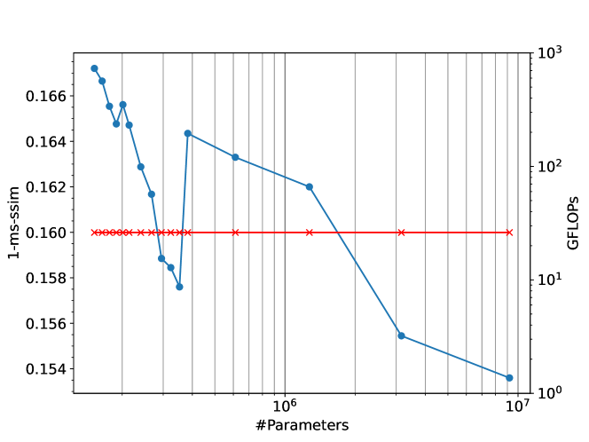
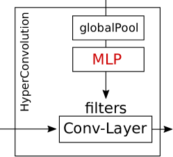
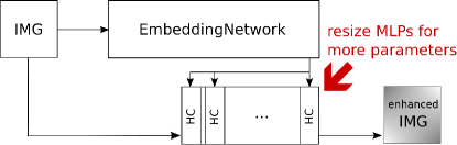
Figure 1: It is possible to improve generalization in a ConvNet at near constant FLOP count with increasing over-parametrization, by using HyperConvolutions (HC) with predicted filters. Usually the ratio of parameters to FLOPs is fixed in convolution layers. The MLPs in the HC can increase this ratio.

In recent years we have seen exceptional progress in computational image enhancement, fueled among others by better processing pipelines [4], problem formulations [15] and increasingly powerful deep learning models [19]. The resulting algorithms meet wide-spread interest in the era of mobile phone cameras, whose sensors are small and therefore prone to producing low-quality RAW data (compared to larger sensors).

For the mobile setting however, permissible power consumption is limited. FLOP-count and memory use need to be kept on a budget for practical utility [17]. Similarly in the data-center setting, power consumption and FLOP count of models is a growing concern, for both economical as well as environmental reasons [33]. Unfortunately, in deep learning often larger models are better models [25].

This dilemma can be better understood given the context of two observations. Firstly, in convolution layers FLOP count and parameter count are tied together. The ratio between them is proportional to the input feature-map resolution (see also Sec. 4). Secondly, the classical bias-variance trade off [3] does not fully characterize the generalization behavior of neural networks. For neural networks often optimal generalization occurs in the many parameter limit; i.e. one finds a ‘double-descent’ generalization curve [2] on the plot of test-error vs. parameter count.

If indeed computer vision tasks, and the neural networks used to tackle them, do exhibit this kind of generalization behavior (as e.g. shown in [25]), this spells a problem for constructing ConvNet variants with few FLOPs, because it may be impossible to endow them with sufficiently many parameters.

Fixing this problem by resizing images or giving up translation equivariance seems unappealing, because resolution reduction requires discarding information and translation equivariance is intuitively useful for many computer vision tasks (and necessary for some physics models).

In this paper we propose and investigate an alternative approach to break the FLOP count to parameter count ratio, that preserves translation equivariance and image scale. This approach is predicting convolutional filters from the input image, by way of a HyperNetwork. We show that this allows for double-descent generalization at fixed FLOP count (in the large input image limit) on the example of a fully neural ISP for the Zurich RAW to DSLR data-set [19].

2 Main Idea and Contributions

2.1 Main Idea

The ratio of number of parameters to number of operations in a convolution layer is fixed at a given resolution. It is $2\cdot H\cdot W$, where $H,W$ are the input height and width (see also Sec. 4).

To break this dependency we can either re-scale the input or relax the weight-sharing scheme of the convolution (not apply the same filter everywhere on the input). Both of these approaches have a significant impact on the inductive bias of the resulting layer: Re-scaling the input decreases spatial resolution and relaxing weight-sharing disrupts translation-equivariance.

In this paper we propose a third avenue for modifying this fixed ratio. We use meta-parametrization, parameters that are themselves the results of computations. A hyper-network [11] predicts the convolutional filters of the forward network for each input image. This hyper-network can contain global pooling and fully-connected layers. By re-scaling these fully-connected layers, we can change the number of parameters of the overall network. Because the fully-connected layers do not scale with input image size, in the limit of large images, their impact on FLOP count is negligible. See Fig. 1 for an illustration of the main idea.

As a result we can build networks that simultaneously 1) operate at full resolution, 2) keep translation equivariance, 3) have high parameter count, 4) have low FLOP count.

2.2 Contributions

The main contributions of this paper can be summarized as follows:

• We identify the problem of fixed FLOP to parameter ratio for building efficient ConvNets.

• We investigate generalization behavior as a function of parameter count at fixed FLOP count in ConvNets (Sec. 5.2).

• We outperform previous state-of-the-art architectures in SSIM [6] and MS-SSIM [19] on the Zurich RAW to DSLR task at $>10\times$ fewer FLOPs (Sec. 5.3)

• We reduce the FLOP count of the well-established VDN [37] by $>6\times$ without loss in fidelity on the SIDD benchmark [1] (Sec. 5.4) with a ‘drop-in’ replacement for convolution layers (code in appendix).

3 Related Work

3.1 Double Descent Generalization

Double descent generalization was observed in [2], has been confirmed in different architectures [25] and is, in some settings, theoretically well understood [12]. It refers to a particular dependency of generalization error (or empirical error on a test set) on the number of free parameters in some machine-learning models. Namely, that with increasing number of parameters, the generalization error first goes down, then up and then down again (hence ‘double descent’). See Fig. 2. In models that have this behavior, the best performing models are the ones with the most parameters. These models are said to interpolate the data.

In this paper we point out that interpolating FLOP-efficient ConvNets may be possible, by increasing their parameter density (per FLOP) using HyperNetworks.

Figure 2: Cartoon of the ‘double descent’ generalization often observed in neural networks.

3.2 HyperNetworks and Dynamic Networks

HyperNetworks [11, 29] are neural networks in which some weights (or convolutional filters) are the outputs of a neural (sub-)network. More generally neural networks, whose parameters are the results of computations have been proposed in many different forms, e.g. [32, 10]. Dynamic convolutions [23] and dynamic filter networks [20] propose predicting the filters of a ConvNet or convolution layer from an input image or feature maps. [24] uses HyperNetworks to prune (sparsify) a network, which is an alternative approach to using HyperNetworks to boost efficiency.

In this paper we apply such HyperNetworks (dynamic convolutions) and re-scale their fully-connected layers to break the fixed parameter to FLOP ratio of ConvNets.

3.3 CondConv

Conditional convolutions [36] are a recent variant of dynamic filter networks, in which the filter prediction has a particular form. Namely filters are predicted as weighted sums of several meta-filters; the weights in this weighted sum are predicted from feature-maps. In this case the HyperNetwork is kept small to reduce computational burden.

In contrast to this, we deliberately increase the size of this HyperNetwork, so that parameter numbers increase.

3.4 Vision Transformer

Recently it has been shown that transformer architectures can achieve excellent accuracy on computer vision tasks [8]. Similar to the HyperNetwork-backed convolutions we use in this paper, transformers have a higher parameter to FLOP ratio than standard ConvNets. However, they have different inherent inductive biases (e.g. transformers do not exhibit translation equivariance).

3.5 Efficient ConvNets

There is a wide literature on designing efficient ConvNets. An excellent overview is given in [7]. To our knowledge ours is the first paper pointing out the potential for reducing FLOPs by decoupling FLOP-count form parameter-count in ConvNets.

4 Method

In this section we describe the basic HyperNetwork component that we will use repeatedly for our experiments. We term this block a HyperConvolution.

For an illustration see Fig. 1, for a pseudo-code description Alg. 1, for code see the appendix. The functions in the pseudo-code are self-explanatory (modeled after pytorch functions), with the exception of ‘normalize’, which ensures that the resulting filter’s magnitude lie in a range that prevents fast activation explosion or decay at increasing depth; see Sec. 4.1 for details.

Algorithm 1 HyperConvolution

1:function HyperConvolution (I, F, n, $f_{W}$, $f_{H}$)

2:// I: forward feature maps, shape(I): $(N,C_{\text{I}},H_{\text{I}},W_{\text{I}})$

3:// F: filter feature maps, shape(F): $(N,C_{\text{F}},H_{\text{F}},W_{\text{F}})$

4:// n: size of MLP layers

5:// $f_{W}$, $f_{H}$: width and height of predicted filter

6:// returns: $\text{I}_{\text{out}}$, shape($\text{I}_{\text{out}}$): $(N,C_{\text{O}},H_{\text{I}},W_{\text{I}})$

7:$\text{F}_{\text{flat}}\leftarrow\text{globalMaxPool(F).flatten()}$

8:$f_{\text{flat}}\leftarrow\text{MLP}_{\text{n}}(\text{F}_{\text{flat}})$

9:$f\leftarrow f_{\text{flat}}$.reshape$(N\times C_{I}$,$C_{O}$,$f_{W}$,$f_{H}$)

10:$f\leftarrow\text{normalize}(f)+f_{\text{bias}}$

11:$\text{I}_{\text{grouped}}\leftarrow\text{I}$.reshape$(1,N\times C_{\text{I}},H_{\text{I}},W_{\text{I}}$)

12:$\text{I}_{\text{out}}\leftarrow\text{GroupConv}(\text{I}_{\text{grouped}},f,\text{n}_{\text{groups}}=N,\text{pad=Same})$

13:return $\text{I}_{\text{out}}$.reshape$(N,C_{\text{O}},H_{\text{I}},W_{\text{I}})$

The HyperConvolution block takes two inputs: A ‘forward input’ $I$ which it will convolve with some filters (and then output) and secondly a ‘filter input’ $F$ from which filters are computed (with which to convolve the forward input). The $F$ is max-pooled to size $1\times 1$, and then fed into a multi-layer perceptron (MLP). The output layer of this MLP is sized such that it can be reshaped into the required convolutional filters.

Note that the size of the hidden layers in the MLP impacts the number of parameters of the HyperConvolution block, but the number of FLOPs required for it, does not scale with the input image size. For a typically sized input image (hundreds to thousands of pixels per dimension) and a hidden layer in the range of hundreds to thousands of neurons, the FLOPs required for the MLP become negligible. Due to this, resizing the MLP allows increasing parameter count at minor impact on FLOPs.

Further note that each sample in the forward input batch is convolved with its own set of filters. In practice this means that the convolution is best implemented as a grouped convolution (see Alg.1).

In numbers, the ratio of FLOPs to parameters in a HyperConvolution block is

$$\frac{N_{\text{FLOP}}}{N_{\text{Param}}}=\frac{2\cdot C_{\text{in}}\cdot C_{\text{out}}\cdot f_{H}\cdot f_{W}\cdot W\cdot H+N_{\text{FLOP-MLP}}}{C_{\text{in}}\cdot C_{\text{out}}\cdot f_{H}\cdot f_{W}+N_{\text{Param-MLP}}}$$ (1)

Note that $N_{\text{Param-MLP}}$ and $N_{\text{FLOP-MLP}}$ are independent of the input resolution and for an MLP without biases $N_{\text{Param-MLP}}/N_{\text{FLOP-MLP}}=1/2$ (if we count one multiply-accumulate as 2 FLOPs). In contrast for a standard convolution layer this is

$$\frac{N_{\text{FLOP}}}{N_{\text{Param}}} = \frac{2\cdot C_{\text{in}}\cdot C_{\text{out}}\cdot f_{H}\cdot f_{W}\cdot W\cdot H}{C_{\text{in}}\cdot C_{\text{out}}\cdot f_{H}\cdot f_{W}}$$ (2)

$$= 2\cdot W\cdot H$$

In the standard convolution, clearly this ratio can only be changed, by modifying the input resolution.

4.1 Normalization of Predicted Filters

In standard neural networks it has been observed that it is helpful for stable convergence of training to initialize weight matrices (or convolution filters) such that the variance of activations propagating through the network does not grow or decay too quickly [9]. For our HyperConvolution layers we ensure this by normalizing the output of the MLPs given in the HyperConvolution Alg. 1 (the notation in the following is consistent with that algorithm).

We assume the reshaped output $f$ of the MLP is normally distributed

$$f\sim\mathcal{N}(0,1)$$ (3)

Aiming for ‘He initialization’ [13] we need to scale this with $\sqrt{2/\text{fan-in}}=\sqrt{2/(C_{\text{in}}\cdot f_{W}\cdot f_{H})}$. We can also achieve the desired variance by the following normalization:

$$f\leftarrow f\cdot\frac{\sqrt{2\cdot f_{W}\cdot f_{H}}}{\sqrt{C_{\text{in}}\cdot\pi/2}\cdot|f|.\text{sum}([2,3])}$$ (4)

where we use that the mean of the half-normal distribution is $\sigma\sqrt{2/\pi}$ such that

$$\mathbb{E}\left[|f|.\text{sum}([2,3])\right]=\sqrt{2/\pi}\cdot f_{W}\cdot f_{H}$$ (5)

The normalization of Eq. 4 further fixes the L1-norm of each filter to 1. This has an effect similar to Instance-Normalization, in that output channels have approximately the same magnitude.

4.2 Memory Requirements and Parameters

For standard convolution layers increasing the number of parameters, will increase the memory requirements (RAM usage) of the network. The dominating contributor to this are the feature maps (not the filters) in most standard architectures.

When using HyperConvolutions, two networks with the same number of parameters can have very different memory requirements. Consider as an example one network with many channels per HyperConvolution and few hidden units in the MLP, and another with few channels and many hidden units in the MLP.

The networks we use in this paper have comparatively low memory requirements, although they have many parameters (see Tab. 1). This is due to the fact that our networks have comparatively fewer feature maps (or channels per convolution).

4.3 HyperConvolution as a Non-local Method

A different motivation for the use of HyperConvolutions is that they incorporate global information into the high-resolution pathway of a ConvNet through the HyperNetwork that predicts convolution filters. Non-local information is well-known to be useful in deep learning approaches to image processing [34].

Furthermore, a Hyper-Convolution layer bears some similarity to ‘classical’ (non-deep-learning) non-local methods: Both BM3d [5] and a Hyper-Convolution layer with sigmoid activation function perform the following operation on an abstract level: From an input image $I$ feature patches $P$ are computed followed by a similarity between subsections of $I$ and $P$. Here the commonality ends. In our approach, the patches $P$ are the predicted convolution filters and the similarity is the sigmoid of a dot-product, where for BM3d $P$ are image sub-blocks and the similarity is a carefully crafted block-distance measure. Nevertheless this additionally motivates the use of Hyper-Convolutions from a perspective of inductive biases.

Figure 3: Double Descent curve for our U-Net with HyperConvolutions: Interpolating generalization at constant FLOPs by increasing MLP size.

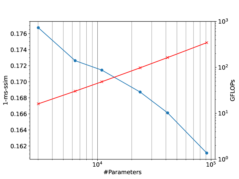
Figure 4: Corresponding curve for the same U-Net with standard convolutions. FLOPs grow very large before curve flattens.

Network ($n_{\text{fwd}},n_{\text{embed}},n_{\text{hid}}$)	FLOPs	Parameters	CPU time	Max. Conv. Mem.	PSNR	MS-SSIM	SSIM
PyNet [19]	43 T	47 M	120 s	29.7 Gb	21.19	0.8620	-
PyNet-CA [21]	45 T	51 M	131 s	32.8 Gb	21.22	0.8549	0.7360
AWNet 4-channel [6]	9.4 T	52 M	55 s	27.8 Gb	21.38	0.8590	0.7451
SPADE [26] *	0.8 T*	97 M*	-	-	20.96	0.8586	-
DPED [16] *	1.4 T*	4 M*	-	-	20.67	0.8560	-
UNet [28] *	3.9 T*	17 M*	-	-	20.81	0.8545	-
Ours (96, n/a, n/a) no HC	1.3 T	0.4 M	11 s	3.8 Gb	19.93	0.8463	0.7213
Ours (64, n/a, n/a) no HC	0.6 T	0.2 M	7 s	2.6 Gb	19.82	0.8446	0.7185
Ours (64, 32, 2048)	0.7 T	276 M	12 s	3.4 Gb	21.37	0.8640	0.7509
Ours (32, 32, 2048)	0.3 T	95 M	6 s	2.2 Gb	21.11	0.8618	0.7466
Ours (32, 16, 2048)	0.2 T	90 M	5 s	1.8 Gb	21.15	0.8617	0.7471
Ours (8, 32, 4000)	0.1 T	113 M	3 s	1.3 Gb	20.22	0.8428	0.7232

Table 1: Performance comparison on ZRR [19] of the proposed networks and state-of-the-art (single networks, w/o ensembling). FLOPs are computed assuming a 12.6Mpix input. No HC indicates ablation experiments with standard convolutions in place of the HyperConvolution. The first four columns are only given, where we had access to a pre-trained model. The two best results are marked in bold, the best in red. *Results reproted in [19], FLOPs and parameters estimated by hand.

Network	FLOPS	Param.s	CPU time	Max. Conv. Mem.	PSNR (valid / test)	SSIM (valid / test)
VDN	9.5 T	7.8 M	3.1 s / MPix	2.3 GB	39.36 / 39.26	0.917 / 0.955
Ours ($n_{\text{channel}}/3$)	1.4 T	55.0 M	1.5 s / MPix	1.0 GB	39.40 / 39.23	0.918 / 0.957
Ours ($n_{\text{channel}}/2$)	2.9 T	119.6 M	2.5 s / MPix	1.4 GB	39.42 / 39.27	0.918 / 0.957

Table 2: Comparison on SIDD [1] of the original VDN [37] and the same network using our HyperConvolutions with fewer channels.

(a)

(b)

(c)

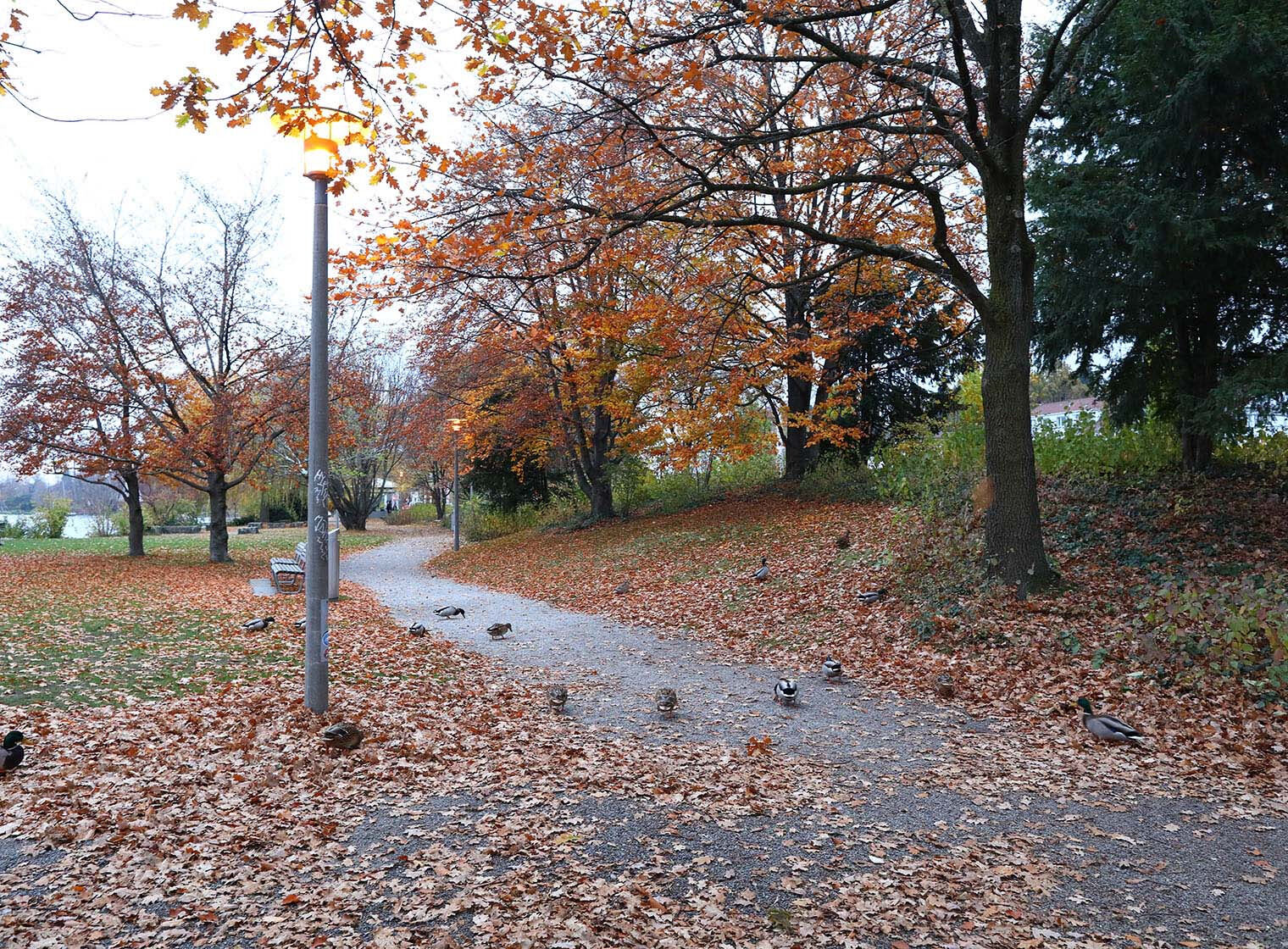
(d)

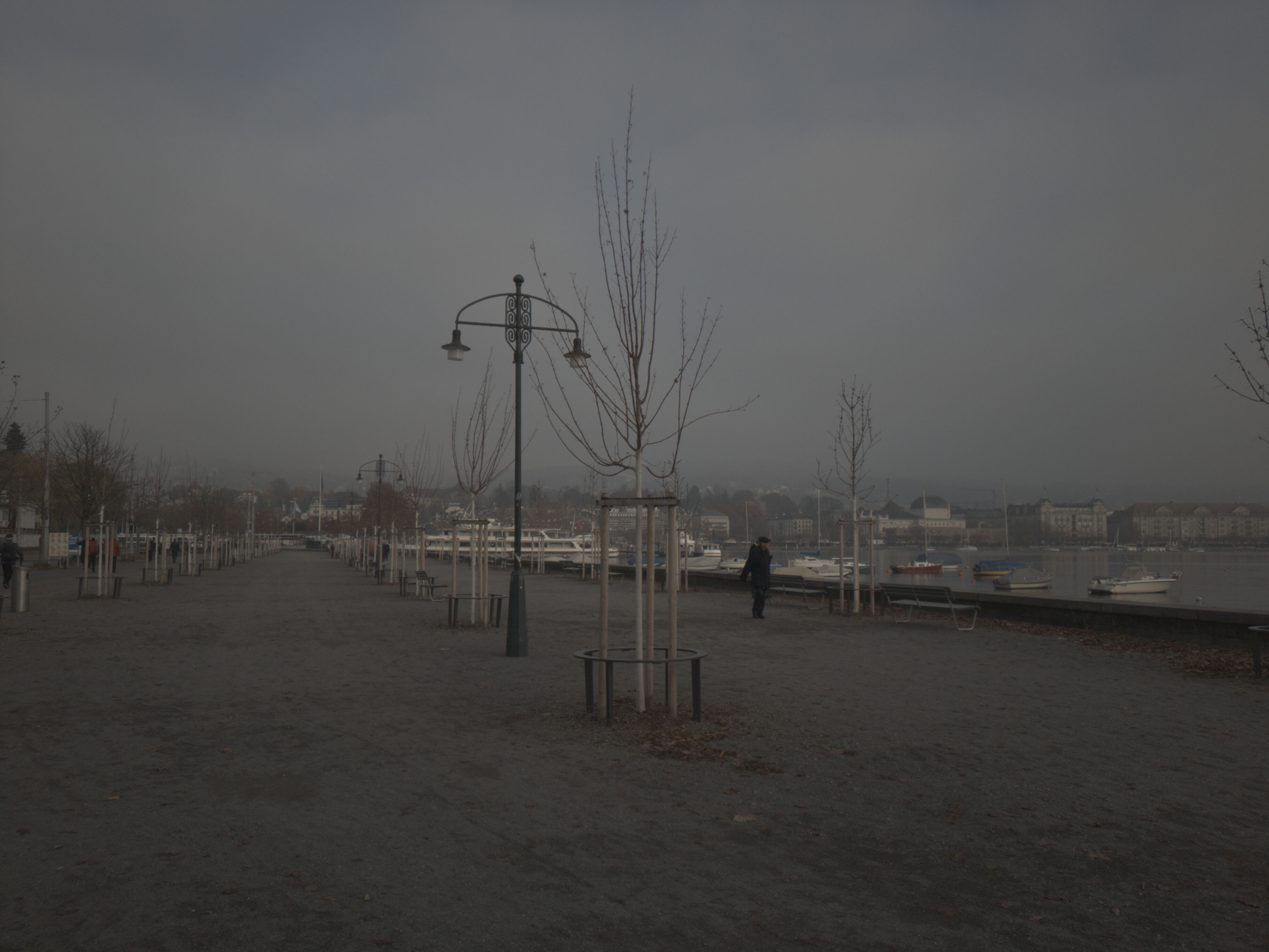
(e)

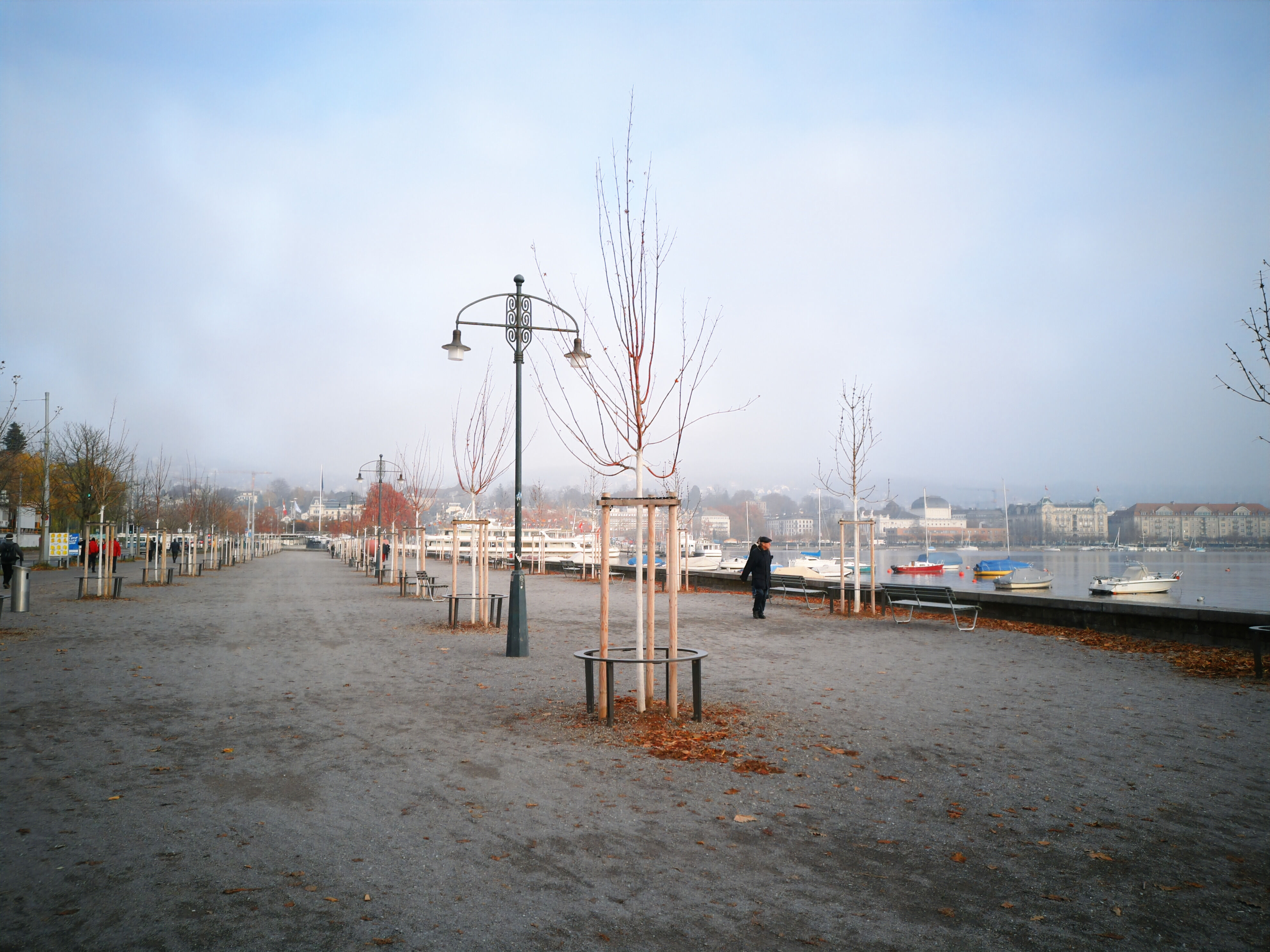
(f)

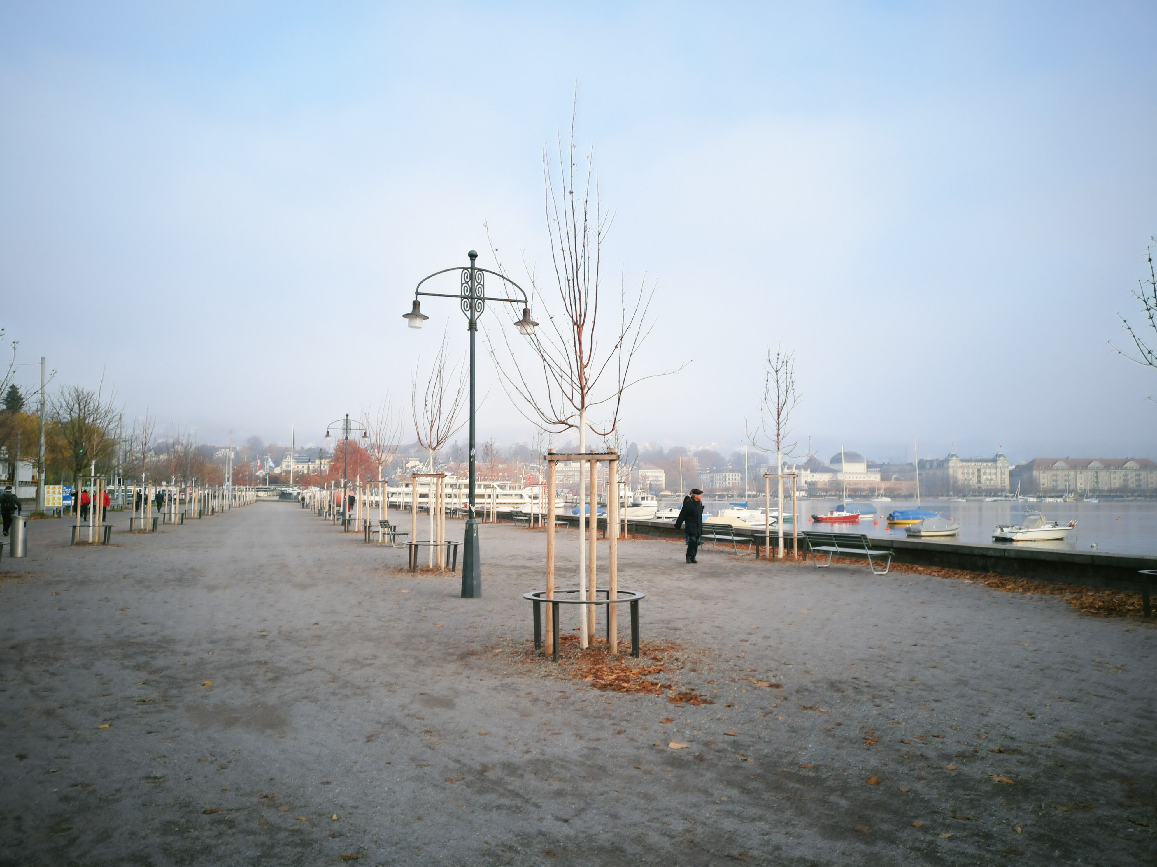
(g)

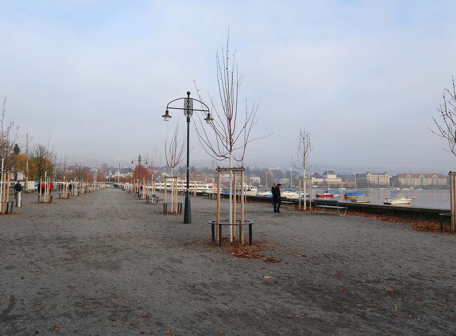
(h)

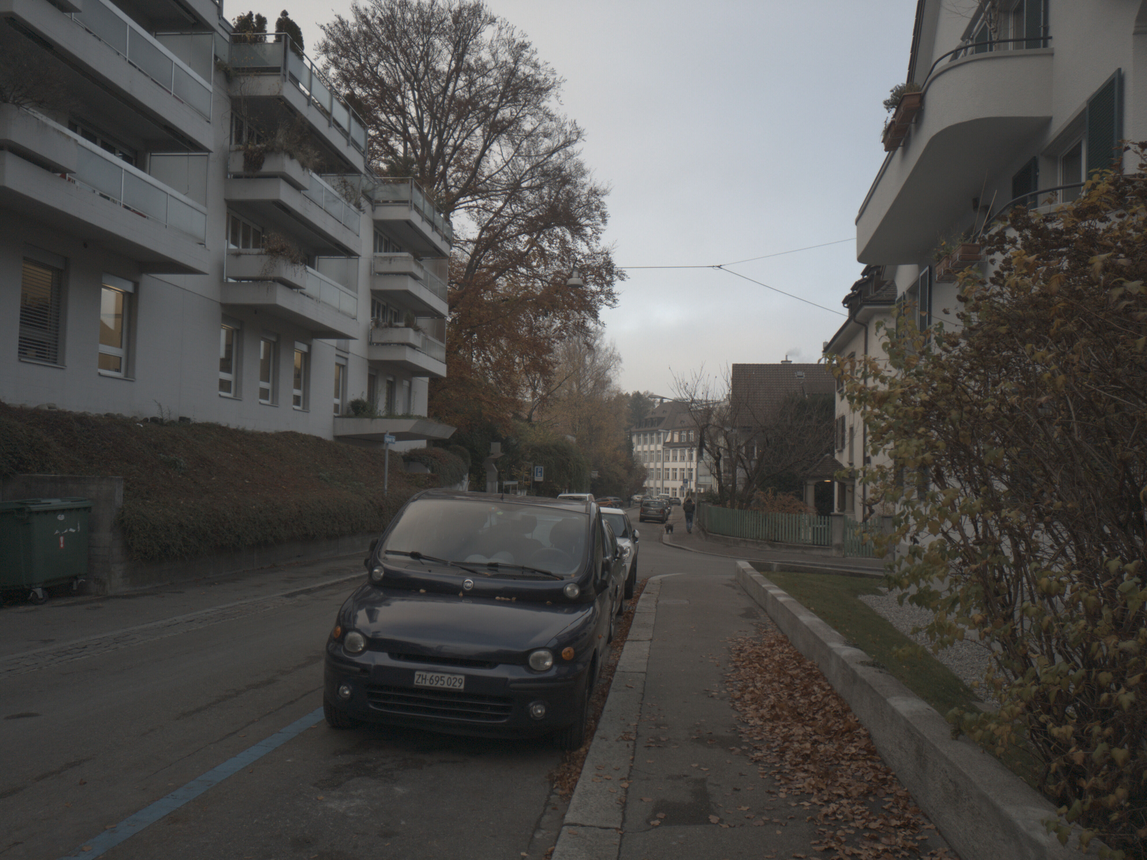
(i)

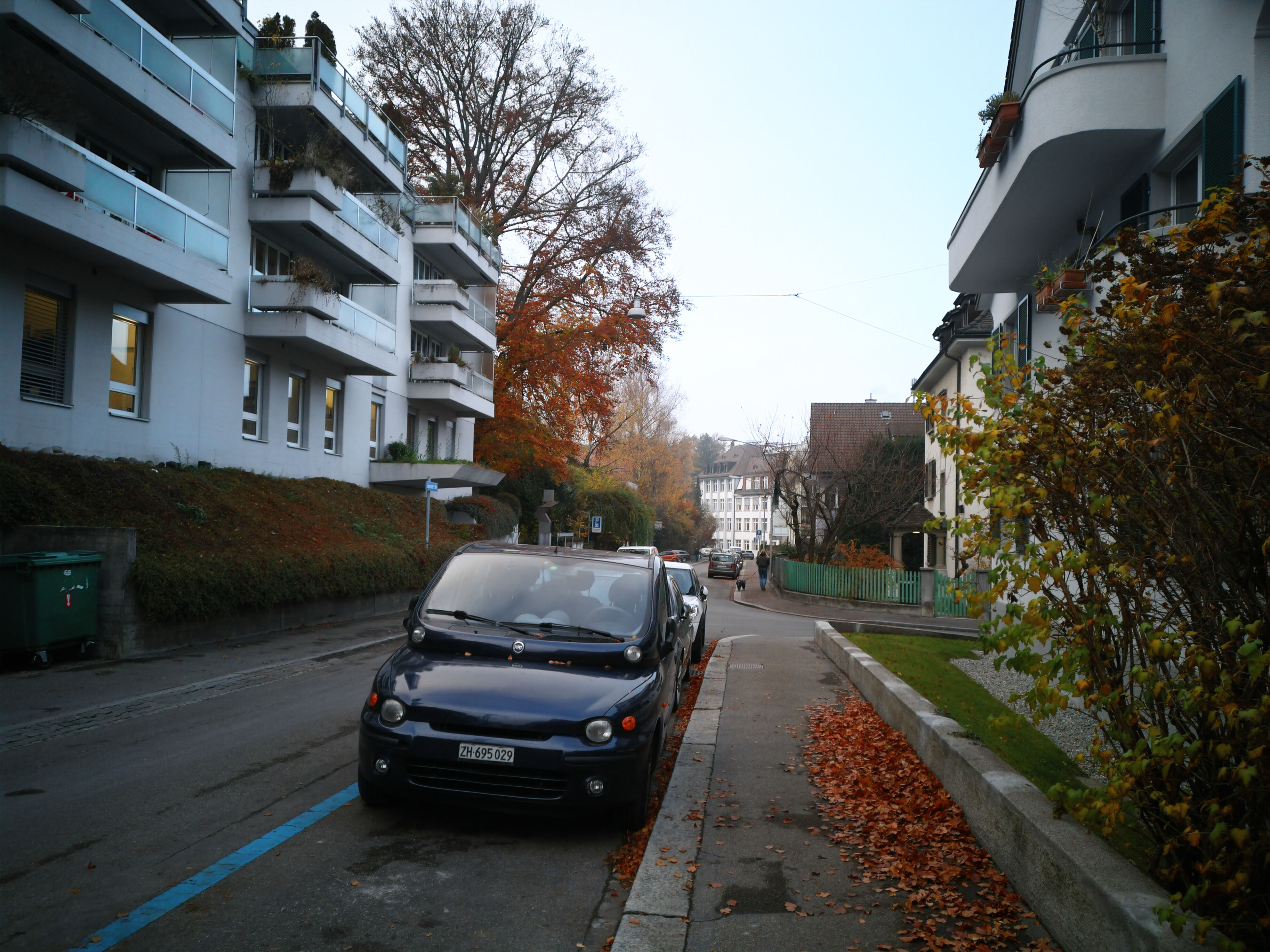
(j)

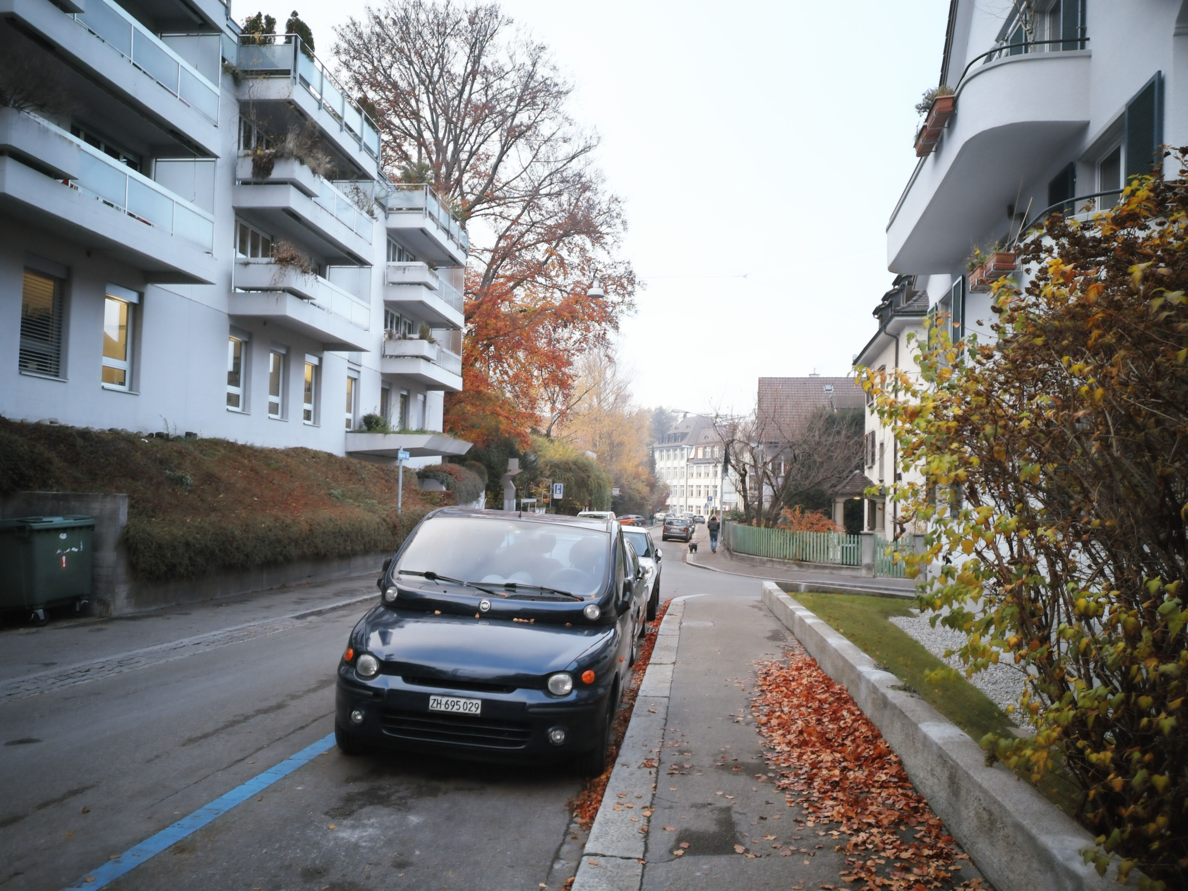
(k)

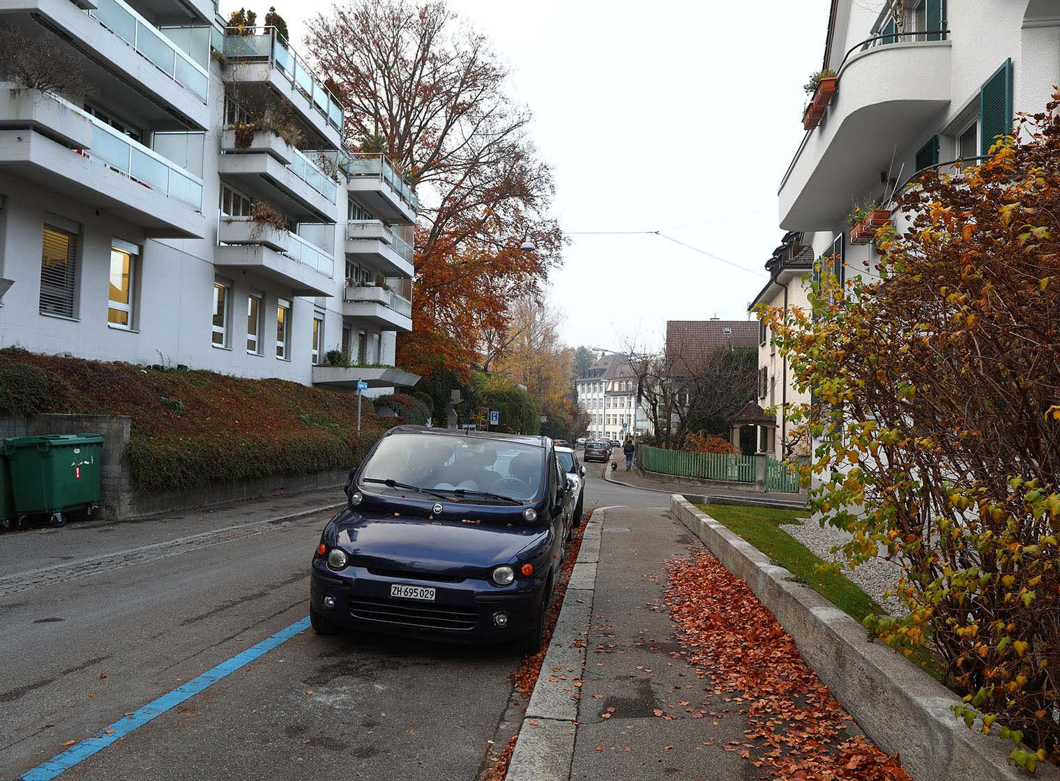
(l)

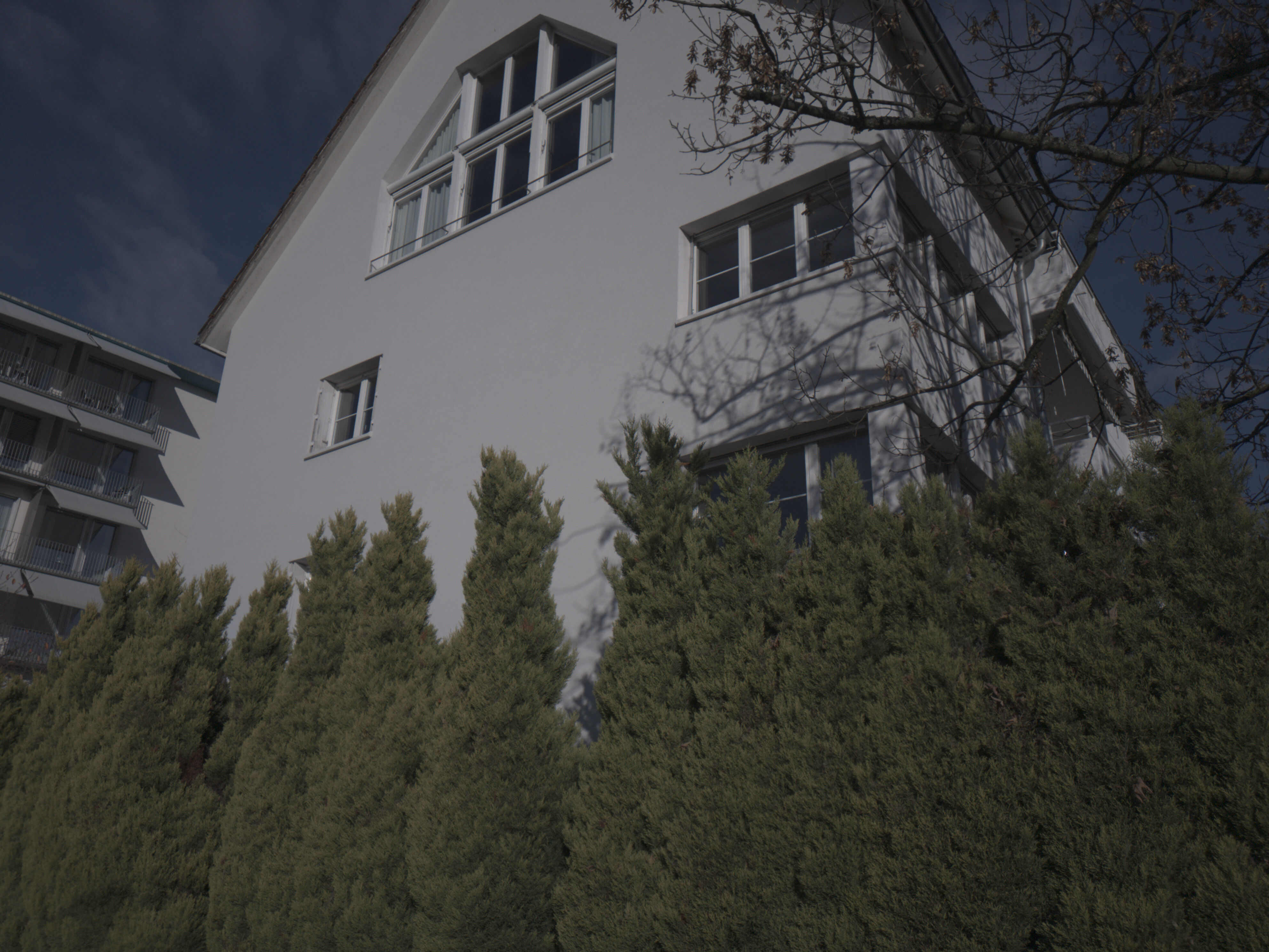
(m) RAW visualized

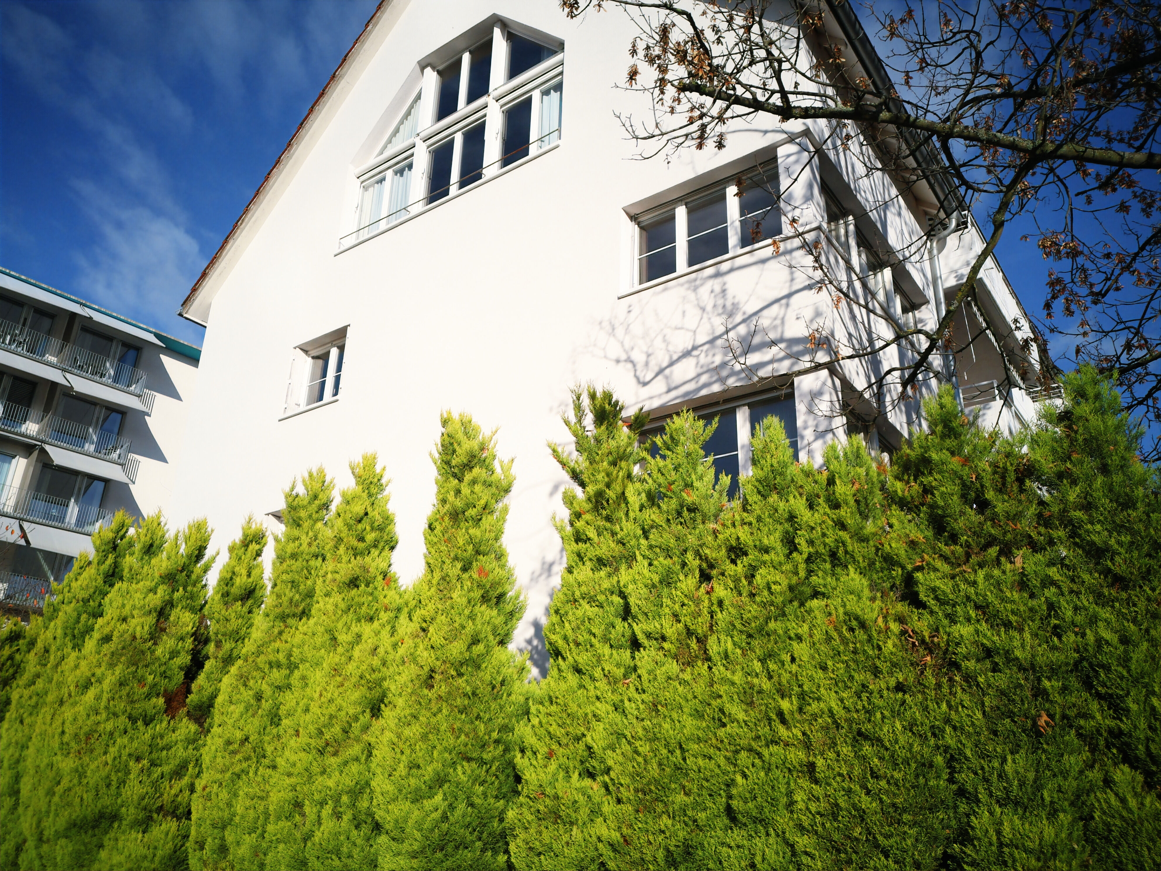
(n) AWNet

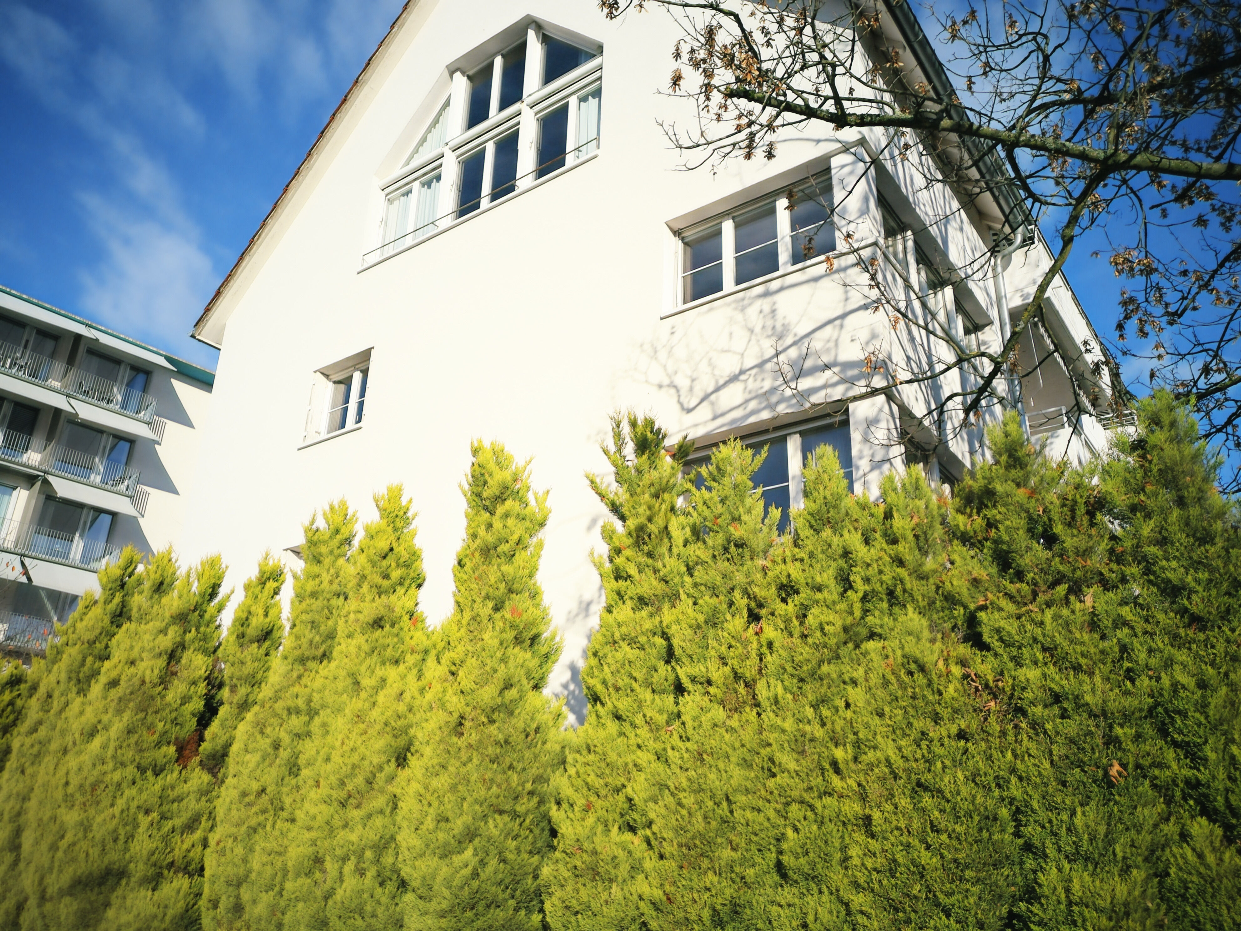
(o) Ours

(p) DSLR (target)

Figure 5: Comparison full images ZRR

(a)

(b)

(c)

(d)

(e)

(f)

(g)

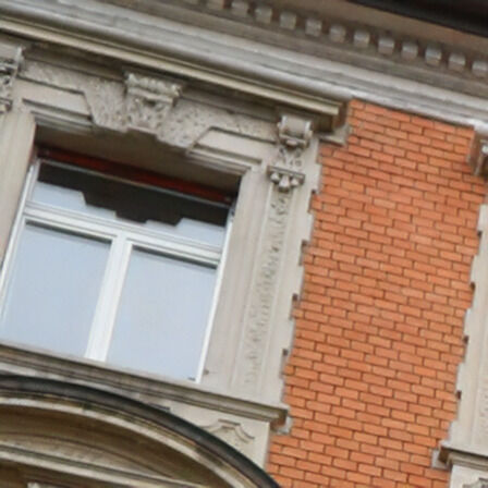
(h)

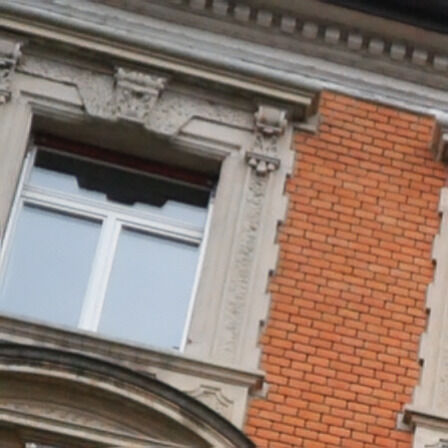
(i)

(j)

(k) RAW

(l) AWNet

(m) PyNet

(n) Ours

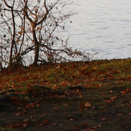
(o) DSLR (target)

Figure 6: Comparison image details

4.4 Drawbacks of this Method

While FLOPs and memory usage (RAM / VRAM) are low, parameter count is increased and therefore model-size and HDD space requirements are increased.

For large batch-sizes and small images, grouped convolutions (used in the HyperConvolution) can be less efficient than standard convolutions (because of potentially limited parallelism).

5 Experiments

In this section we present our experimental findings on the Zurich RAW to DSLR task and the SIDD task. Firstly, we observe the performance of our networks as a function of the scaled size of fully-connected layers in a HyperNetwork, in Sec. 5.2. Secondly, we build a large network making use of the proposed HyperConvolutions and compare to state of the art in Sec. 5.3. Finally, we substitute convolution layers in a VDN [37] for our HyperConvolutions and show matched fidelity at reduced computational cost in Sec. 5.4.

All experiments were run using PyTorch [27]. Training details are given in the appendix, along with code used for the key functionalities described.

5.1 Data-Sets

Zurich Raw to DSLR

We perform our experiments on the Zurich Raw to DSLR data-set [19] (ZRR). This data-set consists of 48’043 image pairs of resolution 448. Each pair contains one RAW image taken with a mobile phone camera (Huawei P20 Pro) and one fully post-processed JPEG output of a high-end DSLR camera (Canon 5D Mark IV). The images in such a pair cover the same scene under the same view-point and can be assumed to be well-aligned. We follow [19] and transform RAW images from shape $(1,448,448)$ to $(4,224,224)$ by transposing the Bayer pattern into the channel dimension.

The task is the prediction of the DSLR output from the mobile phone camera RAW. In doing this, the algorithm must perform the function of the full ISP pipeline, including demoisaicing, denoising, contrast adaptation and white-balancing.

We choose this data-set, because it includes these various aspects in one place and because it decouples the processing pipeline from the network architecture design, which is our primary focus. Furthermore the authors of [19] compare a number of different baseline architectures.

This data-set was featured in the ECCV 2020 AIM Learned Smartphone ISP Challenge [18]. At the time of writing we could find sufficient detail on [6] and [21] publicly available for a comparison of single network fidelity and computational cost.

Smartphone Image Denoising Dataset

SIDD-Medium [1] is a widely used image denoising dataset consisting of 320 image pairs of noisy and ground-truth images collected from an array of 5 smartphone cameras in various illumination settings. There are two variants, one using RAW input the other sRBG input, in both the aim is to predict a denoised sRGB output. To complement our experiments on ZRR, we use the sRBG to sRGB variant.

5.2 Double-Descent Generalization

In this series of experiments we take networks containing HyperConvolutions and vary the number of hidden units in the MLP inside the HyperConvolutions. Furthermore we take standard ConvNets with the same architecture and vary the number of channels in hidden layers.

We are interested in two things: 1) As a function of the number of parameters, how does the generalization error change? 2) As a function of the number of parameters, how does the number of FLOPs the network requires change?

Our goal is to find out, whether it is possible to decrease generalization error without needing to increase FLOPs. This is motivated by the observation that many networks generalize better, when they have more parameters (see Sec.3.1) and the realization that HyperConvolutions can break the fixed parameter to FLOP ratio of standard convolutions (see Sec. 4)

5.2.1 Network Layout

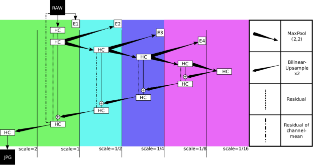
Figure 7: Layout of the UNet-like architecture. The boxes labeled ‘E’ are placeholders for embedding networks. The colored backdrop indicates which embedding network E gives the filter input to a given HyperConvolution HC.

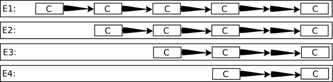
Figure 8: Layouts of embedding networks. ‘C’ stands for $3\times 3$ convolution layers.

We run this experiment for a UNet-like architecture [28].

In this UNet, each occurrence of a convolutional layer is replaced with a HyperConvolution. The number of feature maps in these layers is proportional to $n_{\text{fwd}}$. The filter input to this HyperConvolution is computed by embedding networks (various ones at different scales). The number of feature maps in the layers of all our embedding networks start at $n_{\text{embed}}$ and double at each subsequent layer. Finally $n_{\text{hid}}$ indicates the number of units in the two hidden layers of the MLP that predicts the filters in each HyperConvolution. For an illustration see Fig. 7, for code see the appendix.

All convolutions and HyperConvolutions use filter size $3\times 3$ and the GELU [14] non-linearity, except for the first two HyperConvolution layers which use a hard-sigmoid. We set $n_{\text{fwd}}=8$ and $n_{\text{embed}}=8$. Further details are given in the appendix.

Note that whenever we report FLOPs and parameter numbers we count both the forward network, as well as the filter prediction network.

5.2.2 Results

Figs. 3, 4 show as a function of the number of parameters the test error (1-MS-SSIM) on ZRR and the FLOPs of the considered network and the same network without HyperConvolution.

The proposed HyperConvolution exhibits a generalization curve consistent with double-descent generalization as we increase number of units in the MLP, at negligible FLOP-count increase. Further we see that with standard convolutions the FLOP-count increases steeply with decreasing generalization error, and that at the same FLOP count the over-parameterized HyperConvolution network performs much better.

A plausible underlying explanation for these observations is that the number of parameters (the amount of information the network can store about the training data) is the limiting factor in the learning process. This motivates the development of mechanisms to increase parameter-density in ConvNets like the one given in this paper.

5.3 Large Network

In this experiment we build a larger network of the same layout as given in Fig. 7 and compare its performance to state-of-the-art architectures trained on the same input.

5.3.1 Results

In Tab. 1 we list performance metrics of several network sizes alongside current state-of-the-art. The various networks listed as ‘Ours’ are variants with different settings of $n_{\text{fwd}}$, $n_{\text{embed}}$ and $n_{\text{hid}}$.

CPU time was measured by running a single full-scale image through the evaluation code (where available) on a Ryzen 3700x CPU. The given memory usage is the maximal memory use the pytorch-profiler reports for a convolution. We counted FLOPs using the pytorch-flops-counter.

Two observations are of particular note. Firstly, our largest network exceeds SSIM and MS-SSIM of much more costly networks (in terms of compute time, FLOP count, and memory use). Secondly, the ‘forward’ network used here is comparatively small.

The second observation raises the question, whether there is a limit beyond which decreasing $n_{\text{fwd}}$ (the width of the forward network) cannot be compensated for, by increasing $n_{\text{hid}}$ (the size of the MLPs in the HyperConvolutions). To answer this question we run a further experiment with $n_{\text{fwd}}=8$ and $n_{\text{hid}}=4000$ (all else the same). We find that this network under-performs compared to the wider networks with fewer parameters (see Tab. 1).

This indicates that it is not sufficient to have many parameters. We speculate that in a network with very low $n_{\text{fwd}}$, the narrow forward layers form an information bottleneck [30], that prevents sufficient information about the input from propagating through the network to the output (eventhough there would be sufficiently many parameters to ‘interpolate’ the input data-set).

In Figs. 6, 5 we show sample outputs of our network, next to the outputs of prior approaches.

5.4 Efficient Image Denoising

To verify a broader applicability of our proposed method, in this section we follow closely the setup (architecture, loss, training) of a well established method (VDN [37]), but we replace convolution layers with the HyperConvolutions proposed in Sec. 4. The VDN architecture is a variational method where the network predicts from a noisy input both an estimate of the noise-free image and the noise variance per pixel. We test whether a narrower network (fewer channels per layer) with HyperConvolutions can match the fidelity of the standard VDN at reduced computational cost.

The setup is identical to the VDN reference implementation on github (with the exception of a bug-fix relating to learning-rate decay). Each convolution with $c$ channels is replaced with a HyperConvolution layer with $\mathtt{int}(c/3)$ channels (and $\mathtt{int}(c/2)$ channels in a second experiment). The HyperNetwork that predicts the filter of any given HyperConvolution receives the same input as the HyperConvolution itself and consists of a 3-layer CNN, each layer of which has ReLU non-linearity, stride 2, and their respective channel numbers are 32, 64 and 128 (for code consider the appendix).

The results can be found in Table 2. The FLOP count of our modified VDN is ca. $6.8\times$ lower, memory use and CPU time are also reduced. We indicate memory use and CPU time for a 1 MPix Srgb image as is customary for this benchmark and again use a Ryzen 3700x CPU. The validation set results were performed using the VDN reference code, test results come from the SIDD benchmark website (hence difference in SSIM).

In summary, our modified network matches the fidelity of the standard VDN (it is on-par in PSNR and slightly better in SSIM as for the previous task) at substantially reduced computational cost.

6 Discussion

Often machine learning models are evaluated with the perspective that fewer parameters are inherently better. This makes sense given the ‘classical’ bias-variance generalization curve, because in this settings small models with good predictive ability are the ones with the best inductive biases; their structure best models the data.

In the days of interpolating machine learning models, for which parameter abundance (or high dimensionality) is itself a useful inductive bias, it is arguably time to shift our focus to other metrics of complexity, such as memory use and run-time.

A key result of this paper is that more accurate models with more parameters need not have higher memory requirements and computational cost.

7 Conclusions

In this paper we show that additional parameters can improve generalization in ConvNets with minor impact on the compute cost of the network. The central idea is to use HyperNetworks containing fully-connected layers to predict convolutional filters from input images. The FLOP-count of such fully-connected layers does not scale with input image size. This allows increasing parameter count independently from FLOP count in the large image limit. Using this insight we achieve state-of-the-art single-network SSIM and MS-SSIM on the ZRR task with fewer FLOPs and smaller memory footprint than the best previous architectures [19, 6].

To verify the broader applicability of our proposed method, we further demonstrate that its use in the existing network ‘VDN’ [37] can substantially reduce computational cost while matching fidelity in the SIDD task.

For the tasks of denoising and enhancing RAW photos shot with small mobile camera sensors, FLOP-count is crucial for practical utility, as the mobile setting demands conservative energy and time use. Energy-efficiency is also of high relevance when the environmental impact of training deep learning models is considered. Our approach adds a new tool to the repertoire of energy-efficient image enhancement, as well as offering a new avenue of attack on other parameter-count limited tasks.

Appendix: HyperNetworks with Double-Descent Generalization at Fixed FLOP-Count
Enable Fast Neural Image Enhancement

Training Details

Double Descent Plots

In table 3 we list the training hyperparameters. Where multiple values were considered, they are given in braces, with the preferred value in bold. For hyperparameter selection we trained and validated on a subset of the training data and chose the best values.

The loss-functions we use are mean squared error (MSE) and multi-scale structural similarity (MS-SSIM) [35].

Hyperparameter	Value
optimizer	ADAM [22]
batch size	8
learning rate	$\{2e\text{-}6,\mathbb{5e\text{-}6},1e\text{-}5\}$
$\beta_{1}$	$\{0.5,\mathbb{0.7},0.9\}$
$\beta_{2}$	$\{0.9,\mathbb{0.95},0.99\}$
epochs	30
$n_{\text{fwd}}$	8
$n_{\text{embed}}$	8
$n_{\text{hid}}$	varies
loss	MSE + (1-MS-SSIM)

Table 3: Hyperparameters for the double descent experiments. Bold values were used, values in braces were considered for selection. For further details see flow-text.

Large Network

In Tab. 3 we list the training hyperparameters. At epoch 25 we switch from ADAM [22] to SGD. From epoch 20 onward, we add a VGG-loss at every second batch based on VGG-19 [31].

Hyperparameter	Value
optimizer	ADAM [22] and SGD
batch size	4
epochs	30
$n_{\text{fwd}}$	$\{16,32,\mathbb{64}\}$
$n_{\text{embed}}$	$\{16,\mathbb{32}\}$
$n_{\text{hid}}$	2048
loss	MSE + (1 - MS-SSIM) (+ VGG)

Table 4: Hyperparameters for the large network (where different from double descent experiments). Bold values were used, values in braces were considered for selection. For further details see flow-text.

Code

For convenience we provide some key code snippets below. Please consider the license before use.

⬇

Copyright 2021 Lorenz K. Muller, Huawei Technologies

Licensed under the Apache License, Version 2.0 (the "License");

you may not use this file except in compliance with the License.

You may obtain a copy of the License at

http://www.apache.org/licenses/LICENSE-2.0

Unless required by applicable law or agreed to in writing, software

distributed under the License is distributed on an "AS IS" BASIS,

WITHOUT WARRANTIES OR CONDITIONS OF ANY KIND, either express or implied.

See the License for the specific language governing permissions and

limitations under the License.

⬇

class HyperConv(nn.Module):

def __init__(self, n_in_forward, n_in_hyper, n_out, f_size=3, bias=False, gain=False, n_hid=256, decompose=0,

op_count=False):

’’’

␣␣␣␣␣␣␣␣A␣hyper-network␣convolutional␣filter.␣We␣get␣two␣sets␣of␣input␣feature␣maps.␣The␣first␣set␣we␣average␣pool

␣␣␣␣␣␣␣␣over␣the␣whole␣image␣to␣linearly␣predict␣filters.␣These␣filters␣we␣use␣to␣convolve␣the␣second␣set.

␣␣␣␣␣␣␣␣:param␣n_in_forward:␣number␣of␣channels␣of␣the␣input␣to␣be␣fed␣forward

␣␣␣␣␣␣␣␣:param␣n_in_hyper:␣number␣of␣channels␣of␣the␣input␣to␣the␣hyper-network␣layer

␣␣␣␣␣␣␣␣:param␣n_out:␣number␣of␣learned␣filters␣/␣number␣of␣output␣channels

␣␣␣␣␣␣␣␣:param␣f_size:␣size␣of␣the␣learned␣filter

␣␣␣␣␣␣␣␣:param␣bias:␣flag␣to␣add␣bias

␣␣␣␣␣␣␣␣:param␣gain:␣flag␣to␣add␣multiplicative␣bias

␣␣␣␣␣␣␣␣:param␣n_hid:␣size␣of␣the␣hidden␣layers␣in␣the␣MLP

␣␣␣␣␣␣␣␣:param␣decompose:␣if␣>0␣the␣filters␣are␣predicted␣as␣a␣low-rank␣decomposition␣(not␣used␣in␣paper)

␣␣␣␣␣␣␣␣:param␣op_count:␣flag␣to␣enable␣a␣variant␣that␣is␣friendly␣to␣the␣op-counting␣script␣we␣used

␣␣␣␣␣␣␣␣’’’

super(HyperConv, self).__init__()

self.n_in_forward = n_in_forward

self.n_in_hyper = n_in_hyper

self.n_out = n_out

self.f_size = f_size

self.pool = nn.AdaptiveMaxPool2d(1)

self.pad = nn.ReflectionPad2d(f_size // 2)

self.n_hid = n_hid

self.decompose = decompose

self.op_count = op_count

if decompose < 1:

self.outf = nn.Sequential(nn.Linear(n_in_hyper, n_hid),

nn.ReLU(),

nn.Linear(n_hid, n_hid),

nn.ReLU(),

nn.Linear(n_hid, f_size * f_size * n_in_forward * n_out))

else:

self.outf1 = nn.Sequential(nn.Linear(n_in_hyper, n_hid),

nn.ReLU(),

nn.Linear(n_hid, n_hid),

nn.ReLU(),

nn.Linear(n_hid, f_size * f_size * 1 * n_out * decompose))

self.outf2 = nn.Sequential(nn.Linear(n_in_hyper, n_hid),

nn.ReLU(),

nn.Linear(n_hid, n_hid),

nn.ReLU(),

nn.Linear(n_hid, f_size * f_size * n_in_forward * 1 * decompose))

if op_count:

self.fwd_conv = nn.Conv2d(self.n_in_forward,self.n_out,

kernel_size=f_size, groups=1)

self.bias = None if not bias else nn.Sequential(nn.Linear(n_in_hyper, n_out))

self.gain = None if not gain else nn.Sequential(nn.Linear(n_in_hyper, n_out))

self.const_f = nn.Parameter(data=torch.randn([1, n_out, n_in_forward, f_size, f_size])/np.sqrt(self.n_in_forward*f_size*f_size/2)/2, requires_grad=True)

self.norm = np.sqrt(self.n_in_forward * np.pi / f_size / f_size)

def forward(self, x):

’’’

␣␣␣␣␣␣␣␣:param␣x:␣a␣list␣of␣the␣form␣[x_hyper,␣x_forward]

␣␣␣␣␣␣␣␣:return:␣the␣convolved␣x_forward

␣␣␣␣␣␣␣␣’’’

xfilter, xforward = x

# predict a set of conv filters for each sample

f = self.pool(xfilter) # pool over the full image (becomes independent of input image size)

if self.bias is not None:

b = self.bias(f.view(-1, self.n_in_hyper))

b = torch.clamp(b, -.1, .1)

if self.gain is not None:

g = self.gain(f.view(-1, self.n_in_hyper))

g = torch.clamp(g, -.9, .1) + 1.

if not self.decompose:

f = self.outf(f.view(-1, self.n_in_hyper)) # flatten pooled image and pass through linear layer

else:

f1 = self.outf1(f.view(-1, self.n_in_hyper)).view(-1, self.n_out, 1,

self.f_size, self.f_size, self.decompose)

f2 = self.outf2(f.view(-1, self.n_in_hyper)).view(-1, 1, self.n_in_forward,

self.f_size, self.f_size, self.decompose)

f = (f1*f2).mean(5)

f = f / self.norm

f = f.view(-1, self.n_out, self.n_in_forward, self.f_size, self.f_size).contiguous()

f = f / (f.abs().sum([3, 4], keepdims=True) + 1e-12)/2 + self.const_f

# we reflection pad the forward input (to avoid odd looking image boundaries)

xforward = self.pad(xforward)

# here we need to split the batch up, to apply an individual conv-filter to each sample

# we do this using the ’groups’ keyword of the convolution with the appropriate .view

# in essence this does F.conv2d(xforward, predicted_filter) but the filter varies per sample

xf = F.conv2d(

xforward.view(1, xforward.size()[0] * self.n_in_forward, xforward.size(2), xforward.size(3)),

f.view(xforward.size()[0] * self.n_out, self.n_in_forward, self.f_size, self.f_size),

groups=xforward.size()[0])

if self.op_count:

xf = self.fwd_conv(xforward)

xf = xf.view(xforward.size()[0], self.n_out, xf.size(2), xf.size(3))

if self.bias is not None:

xf = xf + b.view(xforward.size()[0], self.n_out, 1, 1)

if self.gain is not None:

xf = xf * g.view(xforward.size()[0], self.n_out, 1, 1)

return xf

Table 5: Code for Hyperconvolution Layer.

⬇

class HyperUNet(nn.Module):

def __init__(self, n_input_channels, n_fwd=32, embed_base=16, n_out=3, n_hid=256, op_count=False):

super(HyperUNet, self).__init__()

self.n_input_channels = n_input_channels

self.n_fwd = n_fwd

self.embed_base = embed_base

# embedding at input scale

self.embed = nn.Sequential(nn.Conv2d(n_input_channels, embed_base, 3, padding=1), # 224

nn.MaxPool2d(2, 2), nn.GELU(),

nn.Conv2d(embed_base, embed_base * 2, 3, padding=1), # 112

nn.MaxPool2d(2, 2), nn.GELU(),

nn.Conv2d(embed_base * 2, embed_base * 4, 3, padding=1), # 56

nn.MaxPool2d(2, 2), nn.GELU(),

nn.Conv2d(embed_base * 4, embed_base * 8, 3, padding=1), # 28

nn.MaxPool2d(4, 4), nn.GELU(),

nn.Conv2d(embed_base * 8, embed_base * 16, 3, padding=1)) # 7

# embedding at input scale // 2

self.embed2 = nn.Sequential(nn.Conv2d(n_fwd, embed_base, 3, padding=1, stride=2), # 112

nn.MaxPool2d(2, 2), nn.GELU(),

nn.Conv2d(embed_base, embed_base * 2, 3, padding=1), # 56

nn.MaxPool2d(2, 2), nn.GELU(),

nn.Conv2d(embed_base * 2, embed_base * 4, 3, padding=1), # 28

nn.MaxPool2d(4, 4), nn.GELU(),

nn.Conv2d(embed_base * 4, embed_base * 8, 3, padding=1)) # 7

# embedding at input scale // 4

self.embed4 = nn.Sequential(nn.Conv2d(n_fwd//2, embed_base//2, 3, padding=1), # 56

nn.MaxPool2d(2, 2), nn.GELU(),

nn.Conv2d(embed_base//2, embed_base * 2, 3, padding=1), # 28

nn.MaxPool2d(4, 4), nn.GELU(),

nn.Conv2d(embed_base * 2, embed_base * 4, 3, padding=1)) # 7

# embedding at input scale // 8

self.embed8 = nn.Sequential(nn.Conv2d(n_fwd//2, embed_base//2, 3, padding=1), # 56

nn.MaxPool2d(4, 4), nn.GELU(),

nn.Conv2d(embed_base//2, embed_base * 2, 3, padding=1)) # 14

# hyper-convs at input scale

self.hyper_conv0 = HyperConv(n_input_channels, embed_base * 16, n_fwd, f_size=3, bias=True, n_hid=n_hid, op_count=op_count)

self.hyper_conv1 = HyperConv(n_fwd, embed_base * 16, n_fwd, bias=True, f_size=3, n_hid=n_hid, op_count=op_count)

self.hyper_conv2 = HyperConv(n_fwd, embed_base * 16, n_fwd, bias=True, f_size=3, n_hid=n_hid, op_count=op_count)

# hyper-convs at input scale *2

self.hyper_conv4 = HyperConv(n_fwd, embed_base * 16, n_out, bias=True, f_size=3, n_hid=n_hid, op_count=op_count)

# hyper-convs at input scale //2

self.hyper_conv1_2 = HyperConv(n_fwd, embed_base * 8, n_fwd//2, bias=True, f_size=3, n_hid=n_hid//2, op_count=op_count)

self.hyper_conv2_2 = HyperConv(n_fwd//2, embed_base * 8, n_fwd, bias=True, f_size=3, n_hid=n_hid//2, op_count=op_count)

# hyper-convs at input scale //4

self.hyper_conv1_4 = HyperConv(n_fwd//2, embed_base * 4, n_fwd//2, bias=True, f_size=3, n_hid=n_hid//2, op_count=op_count)

self.hyper_conv2_4 = HyperConv(n_fwd//2, embed_base * 4, n_fwd//2, bias=True, f_size=3, n_hid=n_hid//2, op_count=op_count)

# hyper-convs at input scale //8

self.hyper_conv1_8 = HyperConv(n_fwd//2, embed_base * 2, n_fwd//2, bias=True, f_size=3, n_hid=n_hid//2, op_count=op_count)

self.hyper_conv2_8 = HyperConv(n_fwd//2, embed_base * 2, n_fwd//2, bias=True, f_size=3, n_hid=n_hid//2, op_count=op_count)

# hyper-convs at input scale //16

self.hyper_conv1_16 = HyperConv(n_fwd//2, embed_base * 2, n_fwd//2, bias=True, f_size=3, n_hid=n_hid//2, op_count=op_count)

# scaling operations

self.pool = nn.MaxPool2d(2, 2)

self.scale = nn.Upsample(scale_factor=2.0, mode=’bilinear’, align_corners=True)

def forward(self, x):

# embed image

e = self.embed(x)

# scale * 1

y = self.hyper_conv0([e, x])

y0 = torch.clamp(y,0,1)

y = self.hyper_conv1([e, y0]) + y0

y0 = torch.clamp(y,0,1)

# scale // 2

y2 = self.pool(y0)

e2 = self.embed2(y0)

y2 = F.gelu(self.hyper_conv1_2([e2, y2]))

# scale // 4

y4 = self.pool(y2)

e4 = self.embed4(y4)

y4 = F.gelu(self.hyper_conv1_4([e4, y4]))

# scale // 8

y8 = self.pool(y4)

e8 = self.embed8(y8)

y8 = F.gelu(self.hyper_conv1_8([e8, y8]))

# scale // 16

y16 = self.pool(y8)

e16 = e8

y16 = F.gelu(self.hyper_conv1_16([e16, y16]))

# scale // 8

y8 = F.gelu(self.hyper_conv2_8([e8, y8 + self.scale(y16)*.25]) + y8)

# scale // 4

y4 = F.gelu(self.hyper_conv2_4([e4, y4 + self.scale(y8)*.25]) + y4)

# scale // 2

y2 = F.gelu(self.hyper_conv2_2([e2, y2 + self.scale(y4)*.25]) + y2.mean(1).unsqueeze(1))

# scale * 1

y = F.gelu(self.hyper_conv2([e, y0 + self.scale(y2)*.25]) + y0)

y = y + x.mean(1).unsqueeze(1)

# scale * 2

y = self.scale(y)

y = self.hyper_conv4([e, y])

return torch.sigmoid(y)

Table 6: Code for UNet-like architecture.

⬇

class HyperConvEmbed(nn.Module):

def __init__(self, n_in_forward, n_out, f_size=3, bias=False, gain=False, n_hid=64):

’’’

␣␣␣␣␣␣␣␣A␣hyper-network␣convolutional␣filter.␣First␣we␣’embed’␣the␣input␣and␣average␣pool

␣␣␣␣␣␣␣␣over␣the␣whole␣image␣predict␣filters.␣These␣filters␣we␣use␣to␣convolve␣the␣original␣input.

␣␣␣␣␣␣␣␣:param␣n_in_forward:␣number␣of␣channels␣of␣the␣input␣to␣be␣fed␣forward

␣␣␣␣␣␣␣␣:param␣n_out:␣number␣of␣learned␣filters␣/␣number␣of␣output␣channels

␣␣␣␣␣␣␣␣:param␣f_size:␣size␣of␣the␣learned␣filter

␣␣␣␣␣␣␣␣:param␣bias:␣flag␣to␣add␣bias

␣␣␣␣␣␣␣␣:param␣gain:␣flag␣to␣add␣multiplicative␣bias

␣␣␣␣␣␣␣␣:param␣n_hid:␣size␣of␣the␣hidden␣layers␣in␣the␣MLP

␣␣␣␣␣␣␣␣’’’

super(HyperConvEmbed, self).__init__()

self.n_in_forward = n_in_forward

self.n_out = n_out

self.f_size = f_size

self.pool = nn.AdaptiveAvgPool2d(1)

self.pad = nn.ReflectionPad2d(f_size // 2)

self.n_hid = n_hid

embed_base = 32

self.n_in_hyper = n_in_hyper = embed_base * 4

self.embed = nn.Sequential(nn.Conv2d(self.n_in_forward, embed_base, 3, padding=1, stride=2),

nn.ReLU(),

nn.Conv2d(embed_base, embed_base * 2, 3, padding=1, stride=2),

nn.ReLU(),

nn.Conv2d(embed_base * 2, embed_base * 4, 3, padding=1, stride=2))

self.outf = nn.Sequential(nn.Linear(n_in_hyper, n_hid),

nn.LeakyReLU(),

nn.Linear(n_hid, n_hid),

nn.LeakyReLU(),

nn.Linear(n_hid, f_size * f_size * n_in_forward * n_out))

self.bias = None if not bias else nn.Sequential(nn.Linear(n_in_hyper, n_out))

self.gain = None if not gain else nn.Sequential(nn.Linear(n_in_hyper, n_out))

self.const_f = nn.Parameter(data=torch.randn([1, n_out, n_in_forward, f_size, f_size]) / np.sqrt(

self.n_in_forward * f_size * f_size / 2) / 2, requires_grad=True)

self.norm = np.sqrt(self.n_in_forward * np.pi / f_size / f_size)

def forward(self, x):

’’’

␣␣␣␣␣␣␣␣:param␣x:␣forward␣input

␣␣␣␣␣␣␣␣:return:␣the␣convolved␣x

␣␣␣␣␣␣␣␣’’’

xfilter = self.embed(x)

xforward = x

# predict a set of conv filters for each sample

f = self.pool(xfilter) # pool over the full image (becomes independent of input image size)

if self.bias is not None:

b = self.bias(f.view(-1, self.n_in_hyper))

b = torch.clamp(b, -.1, .1)

if self.gain is not None:

g = self.gain(f.view(-1, self.n_in_hyper))

g = torch.clamp(g, -.9, .1) + 1.

f = self.outf(f.view(-1, self.n_in_hyper)) # flatten pooled image and pass through linear layer

f = f / self.norm

if xforward.size()[0] != 1:

f = f.view(-1, self.n_out, self.n_in_forward, self.f_size, self.f_size)

f = f / (f.abs().sum((3, 4), keepdim=True) + 1e-12) / 2 + self.const_f

else:

f = f.view(self.n_out, self.n_in_forward, self.f_size, self.f_size)

f = f / (f.abs().sum((2, 3), keepdim=True) + 1e-12) / 2 + self.const_f.squeeze(0)

# we reflection pad the forward input (to avoid odd looking image boundaries)

xforward = self.pad(xforward)

# here we need to split the batch up, to apply an individual conv-filter to each sample

# we do this using the ’groups’ keyword of the convolution with the appropriate .view

# in essence this does F.conv2d(xforward, predicted_filter) but the filter varies per sample

if xforward.size()[0] != 1:

xf = F.conv2d(

xforward.view(1, xforward.size()[0] * self.n_in_forward, xforward.size(2), xforward.size(3)),

f.view(xforward.size()[0] * self.n_out, self.n_in_forward, self.f_size, self.f_size),

groups=xforward.size()[0])

else:

xf = F.conv2d(xforward, f)

xf = xf.view(xforward.size()[0], self.n_out, xf.size(2), xf.size(3))

if self.bias is not None:

xf = xf + b.view(xforward.size()[0], self.n_out, 1, 1)

if self.gain is not None:

xf = xf * g.view(xforward.size()[0], self.n_out, 1, 1)

return xf

Table 7: Code for ‘drop-in’ HyperConvolution layer used in VDN (includes embedding) assuming ‘same’ padding mode.

Large-scale Image outputs

Of our method (compressed due to file-size limitations)

References

- [1] Abdelrahman Abdelhamed, Stephen Lin, and Michael S Brown. A high-quality denoising dataset for smartphone cameras. In Proceedings of the IEEE Conference on Computer Vision and Pattern Recognition, pages 1692–1700, 2018.
- [2] Mikhail Belkin, Daniel Hsu, Siyuan Ma, and Soumik Mandal. Reconciling modern machine learning and the bias-variance trade-off. stat, 1050:28, 2018.
- [3] Christopher M Bishop. Pattern recognition and machine learning. springer, 2006.
- [4] Tim Brooks, Ben Mildenhall, Tianfan Xue, Jiawen Chen, Dillon Sharlet, and Jonathan T Barron. Unprocessing images for learned raw denoising. In Proceedings of the IEEE Conference on Computer Vision and Pattern Recognition, pages 11036–11045, 2019.
- [5] Kostadin Dabov, Alessandro Foi, Vladimir Katkovnik, and Karen Egiazarian. Image denoising with block-matching and 3d filtering. In Image Processing: Algorithms and Systems, Neural Networks, and Machine Learning, volume 6064, page 606414. International Society for Optics and Photonics, 2006.
- [6] Linhui Dai, Xiaohong Liu, Chengqi Li, and Jun Chen. Awnet: Attentive wavelet network for image isp. arXiv preprint arXiv:2008.09228, 2020.
- [7] Lei Deng, Guoqi Li, Song Han, Luping Shi, and Yuan Xie. Model compression and hardware acceleration for neural networks: A comprehensive survey. Proceedings of the IEEE, 108(4):485–532, 2020.
- [8] Alexey Dosovitskiy, Lucas Beyer, Alexander Kolesnikov, Dirk Weissenborn, Xiaohua Zhai, Thomas Unterthiner, Mostafa Dehghani, Matthias Minderer, Georg Heigold, Sylvain Gelly, et al. An image is worth 16x16 words: Transformers for image recognition at scale. arXiv preprint arXiv:2010.11929, 2020.
- [9] Xavier Glorot and Yoshua Bengio. Understanding the difficulty of training deep feedforward neural networks. In Proceedings of the thirteenth international conference on artificial intelligence and statistics, pages 249–256, 2010.
- [10] Faustino Gomez and Jürgen Schmidhuber. Evolving modular fast-weight networks for control. In International Conference on Artificial Neural Networks, pages 383–389. Springer, 2005.
- [11] David Ha, Andrew Dai, and Quoc V Le. Hypernetworks. arXiv preprint arXiv:1609.09106, 2016.
- [12] Trevor Hastie, Andrea Montanari, Saharon Rosset, and Ryan J Tibshirani. Surprises in high-dimensional ridgeless least squares interpolation. arXiv preprint arXiv:1903.08560, 2019.
- [13] Kaiming He, Xiangyu Zhang, Shaoqing Ren, and Jian Sun. Deep residual learning for image recognition. In Proceedings of the IEEE conference on computer vision and pattern recognition, pages 770–778, 2016.
- [14] Dan Hendrycks and Kevin Gimpel. Gaussian error linear units (gelus). arXiv preprint arXiv:1606.08415, 2016.
- [15] Yuanming Hu, Hao He, Chenxi Xu, Baoyuan Wang, and Stephen Lin. Exposure: A white-box photo post-processing framework. ACM Transactions on Graphics (TOG), 37(2):1–17, 2018.
- [16] Andrey Ignatov, Nikolay Kobyshev, Radu Timofte, Kenneth Vanhoey, and Luc Van Gool. Dslr-quality photos on mobile devices with deep convolutional networks. In Proceedings of the IEEE International Conference on Computer Vision, pages 3277–3285, 2017.
- [17] Andrey Ignatov, Radu Timofte, William Chou, Ke Wang, Max Wu, Tim Hartley, and Luc Van Gool. Ai benchmark: Running deep neural networks on android smartphones. In Proceedings of the European conference on computer vision (ECCV), pages 0–0, 2018.
- [18] Andrey Ignatov, Radu Timofte, Zhilu Zhang, Ming Liu, Haolin Wang, Wangmeng Zuo, Jiawei Zhang, Ruimao Zhang, Zhanglin Peng, Sijie Ren, et al. Aim 2020 challenge on learned image signal processing pipeline. arXiv e-prints, pages arXiv–2011, 2020.
- [19] Andrey Ignatov, Luc Van Gool, and Radu Timofte. Replacing mobile camera isp with a single deep learning model. In Proceedings of the IEEE/CVF Conference on Computer Vision and Pattern Recognition Workshops, pages 536–537, 2020.
- [20] Xu Jia, Bert De Brabandere, Tinne Tuytelaars, and Luc V Gool. Dynamic filter networks. In Advances in neural information processing systems, pages 667–675, 2016.
- [21] Byung-Hoon Kim, Joonyoung Song, Jong Chul Ye, and JaeHyun Baek. Pynet-ca: enhanced pynet with channel attention for end-to-end mobile image signal processing. In European Conference on Computer Vision, pages 202–212. Springer, 2020.
- [22] Diederik P Kingma and Jimmy Ba. Adam: A method for stochastic optimization. arXiv preprint arXiv:1412.6980, 2014.
- [23] Benjamin Klein, Lior Wolf, and Yehuda Afek. A dynamic convolutional layer for short range weather prediction. In Proceedings of the IEEE Conference on Computer Vision and Pattern Recognition, pages 4840–4848, 2015.
- [24] Yawei Li, Shuhang Gu, Luc Van Gool, Radu Timofte, et al. Dhp: Differentiable meta pruning via hypernetworks. In European Conference on Computer Vision and Pattern Recognition (ECCV), 2020, 2020.
- [25] Preetum Nakkiran, Gal Kaplun, Yamini Bansal, Tristan Yang, Boaz Barak, and Ilya Sutskever. Deep double descent: Where bigger models and more data hurt. arXiv preprint arXiv:1912.02292, 2019.
- [26] Taesung Park, Ming-Yu Liu, Ting-Chun Wang, and Jun-Yan Zhu. Semantic image synthesis with spatially-adaptive normalization. In Proceedings of the IEEE Conference on Computer Vision and Pattern Recognition, pages 2337–2346, 2019.
- [27] Adam Paszke, Sam Gross, Francisco Massa, Adam Lerer, James Bradbury, Gregory Chanan, Trevor Killeen, Zeming Lin, Natalia Gimelshein, Luca Antiga, et al. Pytorch: An imperative style, high-performance deep learning library. Advances in Neural Information Processing Systems, 32:8026–8037, 2019.
- [28] Olaf Ronneberger, Philipp Fischer, and Thomas Brox. U-net: Convolutional networks for biomedical image segmentation. In International Conference on Medical image computing and computer-assisted intervention, pages 234–241. Springer, 2015.
- [29] Jürgen Schmidhuber. Learning to control fast-weight memories: An alternative to dynamic recurrent networks. Neural Computation, 4(1):131–139, 1992.
- [30] Ravid Shwartz-Ziv and Naftali Tishby. Opening the black box of deep neural networks via information. arXiv preprint arXiv:1703.00810, 2017.
- [31] Karen Simonyan and Andrew Zisserman. Very deep convolutional networks for large-scale image recognition. arXiv preprint arXiv:1409.1556, 2014.
- [32] Kenneth O Stanley and Risto Miikkulainen. Evolving neural networks through augmenting topologies. Evolutionary computation, 10(2):99–127, 2002.
- [33] Emma Strubell, Ananya Ganesh, and Andrew McCallum. Energy and policy considerations for deep learning in nlp. arXiv preprint arXiv:1906.02243, 2019.
- [34] Xiaolong Wang, Ross Girshick, Abhinav Gupta, and Kaiming He. Non-local neural networks. In Proceedings of the IEEE conference on computer vision and pattern recognition, pages 7794–7803, 2018.
- [35] Zhou Wang, Eero P Simoncelli, and Alan C Bovik. Multiscale structural similarity for image quality assessment. In The Thrity-Seventh Asilomar Conference on Signals, Systems & Computers, 2003, volume 2, pages 1398–1402. Ieee, 2003.
- [36] Brandon Yang, Gabriel Bender, Quoc V Le, and Jiquan Ngiam. Condconv: Conditionally parameterized convolutions for efficient inference. In Advances in Neural Information Processing Systems, pages 1307–1318, 2019.
- [37] Zongsheng Yue, Hongwei Yong, Qian Zhao, Lei Zhang, and Deyu Meng. Variational denoising network: Toward blind noise modeling and removal. In The Thirty-third Annual Conference on Neural Information Processing Systems, 2019.