Geometry of fitness landscapes: Peaks, shapes and universal positive epistasis

Abstract

Darwinian evolution is driven by random mutations, genetic recombination (gene shuffling) and selection that favors genotypes with high fitness. For systems where each genotype can be represented as a bitstring of length $L$, an overview of possible evolutionary trajectories is provided by the $L$-cube graph with nodes labeled by genotypes and edges directed toward the genotype with higher fitness. Peaks (sinks in the graphs) are important since a population can get stranded at a suboptimal peak. The fitness landscape is defined by the fitness values of all genotypes in the system. Some notion of curvature is necessary for a more complete analysis of the landscapes, including the effect of recombination. The shape approach uses triangulations (shapes) induced by fitness landscapes. The main topic for this work is the interplay between peak patterns and shapes. Because of constraints on the shapes for $L=3$ imposed by peaks, there are in total 25 possible combinations of peak patterns and shapes. Similar constraints exist for higher $L$. Specifically, we show that the constraints induced by the staircase triangulation can be formulated as a condition of universal positive epistasis, an order relation on the fitness effects of arbitrary sets of mutations that respects the inclusion relation between the corresponding genetic backgrounds. We apply the concept to a large protein fitness landscape for an immunoglobulin-binding protein expressed in Streptococcal bacteria.

AMS Classification]52B20, 51M20, 05E40, 05C20, 92B05

1 Introduction

This work on acyclic cube graphs and triangulations of cubes is motivated by applications to evolutionary biology. Darwinian evolution can many times be analyzed by considering biallelic systems. For a biallelic $L$-locus system, a genotype $g$ can be represented as a bit string of length $L$. The evolutionary potential for a genotype $g$ is measured by its fitness. The fitness landscape $w:\{0,1\}^{L}\mapsto\mathbb{R}_{\geq 0}$ is determined by the fitness values for all $2^{L}$ genotypes dvk14 . Recent approaches to fitness landscapes rely on analyzing $L$-cube graphs and triangulations that are induced by the landscapes Crona2013b .

One can give a complete (informal) description for $L=2$. The four genotypes are denoted $00,10,01,11$. The induced graph on the square is determined by the condition that each arrow points toward the genotype of higher fitness (Figure 1). A Darwinian process starting from the genotype $00$ corresponds to a path that respects the arrows. The graph 1C has two peaks (or sinks), which means that an evolving population can get stranded at a suboptimal peak.

The quantity $\epsilon=w_{11}+w_{00}-w_{10}-w_{01}$ measures the deviation of the fitness landscape from additivity known as epistasis Domingo2019 ; Krug2021 ; Poelwijk2016 . If $\epsilon>0$ the triangulation induced by the fitness landscape divides the square into two triangles $\{00,10,11\}$ and $\{00,01,11\}$. If $\epsilon<0$, the triangles are instead $\{00,10,01\}$ and $\{10,01,11\}$. For an intuitive understanding, if two genotypes do not belong to the same triangle, they could increase their average fitness by swapping positions (informally, $11+00\mapsto 10+01$ increases fitness if $\epsilon<0$).

In general, we assume that the fitness landscape is generic in the sense of BPS:2007 , in particular that no two genotypes have equal fitness. The graph determined by the fitness landscape, or the fitness graph Crona2013a ; dvk09 , is the acyclic $L$-cube graph defined by the condition that each edge is directed toward the genotype of higher fitness.

Following BPS:2007 , let $\Delta$ be the simplex $\{p\in[0,1]^{2^{L}}:\sum p_{g}=1\},$ where $p$ can be interpreted as the frequencies of the genotypes in a population, and $p\cdot w$ measures the average fitness of the population. Let $\rho:\Delta\mapsto[0,1]^{L}$ be the map defined as $\left(\rho(p)\right)_{i}=\sum_{g_{i}=1}p_{g}$. Note that $\rho$ maps gene frequencies to allele frequencies, i.e, to the frequencies of 1’s at a particular locus (or string position). Define

$$\tilde{w}(v)=\max_{p}\{p\cdot w:\rho(p)=v\}\text{ for all }v\in[0,1]^{L}.$$

Then $\tilde{w}$ is a piecewise linear function. The domains of linearity of $\tilde{w}$ define a regular triangulation of $[0,1]^{L}$ (because $w$ is generic triangulations ). The triangulation is called the shape of the fitness landscape. Recent work on triangulations and fitness graphs includes Crona2017 ; Crona2020a ; Crona2020b ; Das2020 ; Eble2019 ; Eble2020 ; GouldE11951 ; Kaznatcheev2019 ; Lienkaemper2018 .

Fitness graphs and shapes encode information of very different nature, and can be considered complementary Crona2013b . However, there is also some overlap in the information. The peak pattern for a fitness landscape refers to the number of peaks and how they are positioned in the graph, up to cube symmetry. Some peak patterns impose constraints on the triangulations for $L=2$ (Figure 1C) and $L=3$ Srivastava . The main topic for this work is the interplay between peak patterns and triangulations. For the reader’s convenience, a dictionary between terms used in biology and mathematics has been provided, see Table 4.

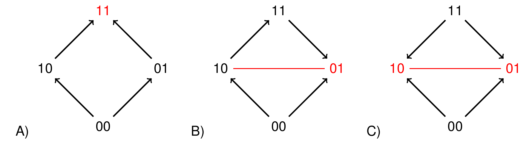
Figure 1: Fitness graphs for two loci under the assumption that $00$ has minimal fitness. If the genotypes are positioned as in the figure, the three types can be characterized as graphs with all arrows up, one arrow down, and two arrows down. Peak genotypes are marked in red. Graphs B) and C) display sign epistasis Weinreich2005 , which means that at least one pair of arrows on parallel edges point in opposite directions. In graph C) sign epistasis is reciprocal Poelwijk2007 . By Observation 2, graphs B) and C) are compatible only with the triangulation indicated by the red lines. Note that for general fitness graphs any genotype can have minimal fitness.

Main Results. For generic fitness landscapes $w:\{0,1\}^{L}\mapsto\mathbb{R}_{\geq 0}$ we compare the induced peak patterns and triangulations. For $L=3$ we show that there are exactly 25 possible combinations of peak patterns and triangulations (Theorem 1). The statistical distribution of peak patterns conditioned on the triangulation is obtained from simulations of random fitness landscapes. For higher $L$ we show that some peak patterns are compatible with all triangulations, whereas other peak patterns are incompatible with almost all triangulations. A peak pattern and a triangulation are referred to as compatible if there exists a fitness landscape that induces both of them.

Additional results for general $L$ can be obtained for fitness landscapes that induce staircase triangulations (Definition 1). We show that these landscapes display a property that we call universal positive epistasis. The property holds if

$$w_{g\cup g^{\prime}}+w_{g\cap g^{\prime}}\geq w_{g}+w_{g^{\prime}}$$ (1)

for all pairs of genotypes $g$ and $g^{\prime}$ interpreted as sets of 1-alleles. It implies that the fitness effect of a given set of mutations on different genetic backgrounds inherits the partial order induced by the subset-superset relation between background genotypes. The conditions (1) characterize the (standard) staircase triangulation. Universal positive epistasis limits the maximal number of peaks in the fitness landscape, and explicit upper bounds are derived for $L=4$ and $L=5$ (Theorem 2). Gröbner bases for staircase triangulations (Section 4) were used for establishing that the bound for $L=4$ is sharp. The analysis of a large empirical data set of fitness interactions between protein substitutions selected for their positive epistatic effects Wu2016 shows a significant overrepresentation of the staircase triangulation.

2 Peak patterns and triangulations for $L=3$

With notation as in the introduction, we consider fitness graphs and triangulations induced by fitness landscapes. The peak set of a fitness graph determines its peak pattern. Two fitness graphs have the same peak pattern if for instance the set of peaks differ by a cube rotation only (see below for a more formal discussion). In particular, all graphs with a single peak have the same peak pattern.

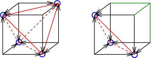
Figure 2: Three locus fitness graphs with 4 and 3 peaks. Face triangulations are indicated by full red lines for the exposed faces and dashed red lines for the hidden faces of the cube. Left panel: For the graph with 4 peaks, the peak pattern fully specifies the triangulation of the faces. The triangulation has to be of type 1 or 2 (these types have identical face triangulations, see Figure 4). Right panel: The presence of three peaks implies that a corner is isolated, which is inconsistent with type 6 triangulations.

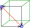
Figure 3: For graphs with two peaks, there are two possible peak patterns, depending on if the distance between the peaks is two or three. If the distance is two, the face triangulation is as indicated by the red line. Both cases are compatible with all six triangulations.

2.1 Classification results for $L=3$

Observation 1.

For $L=3$ there are 5 peak patterns, i.e., four patterns (Figures 2 and 3) in addition to the case with a single peak.

• Fitness graphs have 1-4 peaks.

• The peak pattern is unique if the number of peaks is 1, 3 or 4.

• There are two peak patterns if the number of peaks is 2. The distance between the peaks is either 2 or 3.

A triangulation of the cube can be described as a subdivision of the cube into tetrahedra. It is well known that in the case of the 3-cube only 6 triangulations can arise, up to symmetries, see (triangulations, , Thm. 6.3.10). The possible shapes are illustrated in Figure 4. The graphs below the cubes aid visual interpretations of the triangulations. The nodes of the graphs represent tetrahedra. Two vertices are joined by an edge if the corresponding tetrahedra have a triangle in common, and a shaded region indicates that the tetrahedra share a line segment. The graphs are defined as tight spans dual to the triangulations Herrmann2014 . The corner tetrahedra (see the top row in Figure 4) appear as nodes of degree 1 in the tight spans (i.e., nodes with only one outgoing edge).

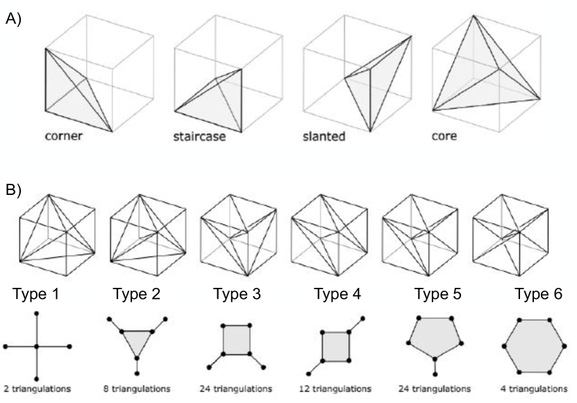
Figure 4: The six types of triangulations of the 3-cube, together with the tight spans dual to the triangulations (modified from Pellerin2018 with permission). Row A) shows the types of simplices that occur in the triangulations.

Theorem 1.

The five peak patterns described in the previous observation, and the six triangulation types, as described in Figure 4, can be combined in 25 ways. Specifically

• Fitness graphs with 4 peaks are compatible with triangulations of type 1 and 2, but not with any other triangulations.

• Fitness graphs with 3 peaks are compatible with triangulations of type 1-5, but not with type 6.

• The remaining three peak patterns are compatible with all six triangulation types.

Before giving a proof we introduce some formal notation for general $L$. The peaks of a fitness graph define a peak pattern for any $L$. Formally, a peak pattern is an equivalence class of peak sets under the action of the hyperoctahedral group of cube symmetries (the group has order $2^{L}L!$). Peak patterns have been enumerated for $L$-cubes up to $L=6$ Oros2022 (see Table 1).

$L$ 2 3 4 5 6 regular triangulations 2 74 87,959,448 - - symmetry classes 1 6 235,277 - - peak patterns 2 5 20 287 519,194

Table 1: The table summarizes known results for the number of regular triangulations and their symmetry classes triangulations ; MR2398786 , and the number of peak patterns Oros2022 for $L$-cubes.

A triangulation of the $L$-cube is a subdivision of the cube into $L$-simplices (i.e., simplices that can be described as the convex hull of $L+1$ affinely independent points), such that any non-empty intersection between simplices are faces of both of them. The triangulation induced by the fitness landscape $w$ was defined in the introduction. In the terminology of triangulations , the triangulation is the projection of the upper envelope of the convex hull of the genotypes lifted by $w$. (For clarity, each genotype $g$ determines a point in $\mathbb{R}^{L+1}$ by regarding its fitness $w_{g}$ as a height coordinate. The triangulation is the projection of the upper faces of the polytope obtained as the convex hull of such points). Triangulations induced by fitness landscapes are defined as regular triangulations. There exist non-regular triangulations for $L\geq 4$ triangulations ; pournin2013 , but such triangulations are not considered in this paper.

For $L=3$, a triangulation divides each side of the cube along a 2-face diagonal, i.e., the diagonal determined by vertices $g,g^{\prime}$ such that $\{g,g^{\prime}\}$ belongs to a tetrahedron in the triangulation. Such diagonals are referred to as induced diagonals. Similarly, for general $L$ a triangulation induces a 2-face diagonal of each 2-face. Specifically, consider a 2-face where the two pairs of vertices with distance two represent genotypes $\{g,g^{\prime}\}$ and $\{h,h^{\prime}\}$. The $g,g^{\prime}$-diagonal is induced by the triangulation if $w_{g}+w_{g^{\prime}}>w_{h}+w_{h^{\prime}}$, which implies that $h$ and $h^{\prime}$ do not belong to the same simplex in the triangulation. The following observation specifies how induced diagonals are constrained by the fitness graph (see Fig. 1 for illustration).

Observation 2.

Consider a 2-face composed of pairs of vertices $\{g,g^{\prime}\}$ and $\{h,h^{\prime}\}$ with distance two. Suppose the fitness graph displays sign epistasis on the 2-face, i.e. at least one of the two pairs of arrows on parallel edges point in opposite directions. Then the induced diagonal connects the arrow heads.

Proof: Assume w.l.o.g. that the antiparallel arrows point from $h^{\prime}$ to $g$ and from $h$ to $g^{\prime}$. This implies that $w_{g}>w_{h^{\prime}}$ and $w_{g^{\prime}}>w_{h}$. Hence $w_{g}+w_{g^{\prime}}>w_{h}+w_{h^{\prime}}$ and the induced diagonal connects $g$ and $g^{\prime}$.

Following triangulations we say that the vertex with the central position in a corner simplex is sliced off by the triangulation (see the bottom left vertex of the corner simplex in Figure 4). For $L=3$ a sliced off vertex belongs to exactly one tetrahedron. In general, a sliced off vertex of the $L$-cube belongs to exactly one simplex of the triangulation (the simplex consists of the vertex itself and its $L$ neighbors).

The proof of Theorem 1 includes an analysis of 2-face diagonals induced by the triangulation. The diagonals marked red in Figures 2 and 3 are induced by the triangulation, because they connect peaks. For the proof it is helpful to introduce a new concept. For arbitrary $L$, we call a genotype $g$ isolated if there is no genotype $g^{\prime}$ such that $\{g,g^{\prime}\}$ belongs to the same simplex and $\|g-g^{\prime}\|=2$, i.e., no induced 2-face diagonal connects $g$ to another genotype.

Remark 1.

If the triangulation slices off a genotype, then the genotype is isolated. However, the converse is not true (see e.g. the Type 2 triangulation in Figure 4).

Observation 3.

For the six triangulation types described in Figure 4,

• Type 1 triangulations have four isolated vertices.

• Type 2 triangulations have four isolated vertices.

• Type 6 triangulations have no isolated vertices.

• All the remaining triangulation types have one or two isolated vertices.

The proof of Theorem 1 relies on the previous observation and simulations summarized in Figure 5 (see Section 2.2 for details on the simulations).

Proof of Theorem 1. If the fitness graph has 4 peaks, then the remaining four genotypes are isolated, which excludes the triangulations of types 3-6 by the previous observation. If the fitness graph has three peaks, then the genotype adjacent to the three peaks is isolated, which excludes the type 6 triangulation. Out of the 30 combinations of peak patterns and triangulations, 5 are excluded as argued. The remaining 25 combinations of peak patterns and triangulations appear with nonzero probability in statistics for randomly generated fitness landscapes (see Figure 5).        $\blacksquare$

Remark 2.

There is an overlap between Theorem 1 and results in Seigal2018 , specifically concerning the case with four peaks (see Corollary 1.4 of Seigal2018 ).

Remark 3.

Theorem 1 describes peak patterns and triangulations that are compatible. A related question concerns if it is possible to combine a particular peak pattern and triangulation in more than one way. Classification results on such combinations would be of interest, but the topic is beyond the scope of this paper.

Open question: For the $L=4$-cube there are 20 peak patterns and 235,277 symmetry classes of regular triangulations (Table 1). Which combinations of peak patterns and triangulations are compatible?

2.2 Peaks and shapes of random fitness landscapes

Generic random fitness landscapes are obtained by assigning independent, identically and continuously distributed random numbers to the genotypes Kauffman1987 . Because peak patterns and fitness graphs are fully determined by the rank order of fitness values, the resulting statistics are independent of the underlying probability distribution. A simple rank order argument shows that the expected number of peaks of a random landscape over $L$ loci is $\frac{2^{L}}{L+1}$, and the variance of the number of peaks is also known Macken1991 . The full distribution of peak patterns for $L=3$ was obtained in SK2014 and is reported in Table 2. Additionally the table shows the distribution of peak patterns over the 54 isomorphism classes of fitness graphs presented in Crona2017 .

Peak pattern	Random landscapes	Isomorphism classes
1 peak	$\frac{3}{14}\approx 0.214$	$\frac{1}{2}=0.5$
2 peaks at distance 2	$\frac{5}{14}\approx 0.357$	$\frac{5}{18}\approx 0.278$
2 peaks at distance 3	$\frac{1}{4}=0.25$	$\frac{4}{27}\approx 0.148$
3 peaks	$\frac{1}{7}\approx 0.143$	$\frac{1}{18}\approx 0.055$
4 peaks (Haldane graph)	$\frac{1}{28}\approx 0.036$	$\frac{1}{54}\approx 0.0185$

Table 2: Distribution of peak patterns for random three-locus landscapes based on SK2014 and Crona2017 . Decimal approximations of the exact rational probabilities are provided for convenience.

Figure 5 shows the distribution of peak patterns conditioned on the triangulation type. The combinations of peak patterns and triangulation types excluded by Theorem 1 are absent in the figure, whereas all other combinations occur with positive probability. In contrast to the statistics of fitness graphs presented in Table 2, these statistics depend on the probability distribution of fitness values Srivastava . Observations similar to the summary in Figure 5, but focused on the number of peaks rather than peak patterns, appeared first in Srivastava . The results in Figure 5 were obtained using the uniform distribution on $[0,1]$ (see Figure 6 for the distribution of triangulation types in this case). Furthermore, it can be seen that the overall ruggedness of the landscapes (as measured, e.g., by the mean number of peaks) decreases systematically going from triangulation type 1 to type 6. A pronounced trend is observed for the patterns with two peaks: Whereas for triangulation type 1 the two peaks are almost exclusively at distance 2, for triangulation type 6 the pattern with two peaks at distance 3 dominates.

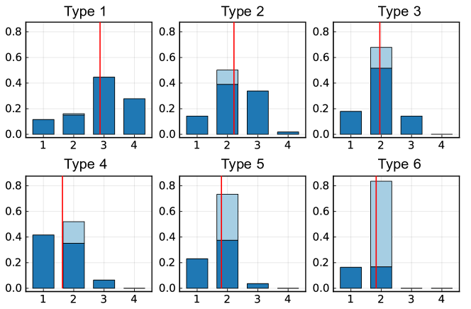
Figure 5: Distribution of the number of peaks for different triangulation types. The fitness values were taken to be uniformly distributed on $[0,1]$. The vertical red lines indicate the mean of the distribution. For unconstrained random three-locus landscapes the mean number of peaks is 2. The light-blue portion of the bars at peak number 2 shows the fraction of landscapes where the two peaks are at distance 3.

3 Higher dimensional fitness landscapes

Throughout the following sections, all triangulations are assumed to be regular. The regularity assumption will not be stated explicitly.

3.1 Extreme peak patterns and triangulations

A counting argument shows that the maximal number of peaks for a fitness graph is $2^{L-1}$. This fact was first observed in haldane_1931 , and we refer to these graphs as Haldane graphs. One can verify that each node in a Haldane graph is either a sink or a source.

Remark 4.

A fitness graph has at most $2^{L-1}$ peaks. For graphs with the maximal number of peaks, each node is either a sink (peak) or a source. All neighbors of sinks are sources, and vice versa.

Among graphs with only one peak, the all arrows up graph is defined as the graph where fitness decreases by distance from the node with maximal fitness (if one draws the graphs as in Figure 1, all arrows point upward).

Observation 4.

The all arrows up graph is compatible with all triangulations.

Proof: The argument relies on the following construction: For a fitness landscape $w$ and a constant $c\in\mathbb{N}$ let

$$w_{g}^{+c}=w_{g}+c\sum_{i=1}^{L}g_{i}.$$

For instance, $w_{{00}}^{+2}=w_{{00}}$, $w_{{10}}^{+2}=w_{{10}}+2$, $w_{{01}}^{+2}=w_{{01}}+2$, $w_{{11}}^{+2}=w_{{11}}+4$. Consider an arbitrary triangulation of the $L$-cube induced by $w$. One verifies that the fitness landscapes $w^{+c}$ and $w$ induce the same triangulation. For sufficiently large $c$, the fitness graph corresponding to $w^{+c}$ is an all arrows up graph, which completes the proof.

Corollary 1.

All triangulations are compatible with some single peaked fitness landscapes.

Type 1 and type 6 triangulations can be considered opposite extremes for $L=3$. The first triangulation slices off four genotypes, i.e., it has four corner simplices, and the latter does not slice off any genotypes. For general $L$, a corner simplex consists of a vertex $g$ (the sliced off vertex) and its $L$ neighbors triangulations . Analogous to the $L=3$ case, corner-cut triangulations are defined as triangulations that have $2^{L-1}$ corner simplices, i.e., the highest number of corner simplices for a given $L$ SCOTTMARA1976170 . Corner-cut triangulations are unique for $L=3$ and $L=4$ but not for general $L$ triangulations .

The staircase triangulation for general $L$ is a direct generalization of the type 6 triangulations. For notational convenience we define the standard staircase triangulation so that each simplex contains the genotypes from a walk of length $L$ from $00\dots 0$ to $11\dots 1$. All $L!$ walks are represented. For instance, for $L=3$ the triangulation is

$$\{000,100,110,111\},\{000,100,101,111\},\{000,010,110,111\},$$

$$\{000,010,011,111\},\{000,001,101,111\},\{000,001,011,111\}.$$

Definition 1.

The standard staircase triangulation consists of $L!$ simplices, such that each simplex contains all genotypes from a walk of length $L$, starting at $00\dots 0$ (the zero-string) and ending at the one-string $11\dots 1$, where the number of $1$’s increases in each step. Any triangulation that is isomorphic to the standard staircase triangulation is referred to as a staircase triangulation.

In particular, there are four isomorphic staircase triangulations for $L=3$ since the pair of vertices that belong to all tetrahedra can be chosen as $\{000,111\}$, $\{100,011\}$, $\{010,101\}$ or $\{001,110\}$.

Also for general $L$, it is useful to consider the induced triangulations of 2-faces. Diagonals connect peaks on the 2-faces for triangulations compatible with Haldane graphs. It follows that the source genotypes are isolated. However, they are not sliced off in general (Remark 1).

Remark 5.

The source genotypes are isolated for Haldane graphs.

Consider the standard staircase triangulation for $L\geq 3$. For any genotype $g$, let $g^{\prime}$ be a genotype obtained by changing two loci (positions) from $1$ to $0$, or two loci from $0$ to $1$. Then $g$ and $g^{\prime}$ belong to the same simplex, which implies that $g$ is not isolated.

Remark 6.

If the fitness landscape induces a staircase triangulation, then there are no isolated genotypes.

Observation 5.

Haldane graphs impose restrictions on triangulations which make them incompatible with some triangulation types. The graphs are compatible with other well studied triangulation types.

1. Triangulations that are compatible with Haldane graphs have $2^{L-1}$ isolated genotypes.

2. Haldane graphs are incompatible with staircase triangulations for $L\geq 3$.

3. For any $L$, there exists a corner cut triangulation that is compatible with the Haldane graph.

Proof: (i) follows from Remark 5. (ii) follows from (i) and Remark 6. For (iii), consider a generic fitness landscape that induces a Haldane graph such that $w_{g}\approx 2$ for half of the genotypes and $w_{g}\approx 1$ for the remaining genotypes. One can verify that the fitness landscape induces a corner-cut triangulation provided the approximations are sufficiently close (each source genotype is sliced off).

We have established that a Haldane graph is compatible with some corner-cut triangulation. A stronger claim would be that any corner-cut triangulation is compatible with the Haldane graph.

Open question: Are all corner-cut triangulations compatible with Haldane graphs?

3.2 Staircase triangulations and universal positive epistasis

It is sometimes convenient to use the set notation for genotypes Das2020 . If the bitstring representing the genotype has a 1 in position $i$, then the set contains the element $i\in{\mathcal{L}}$ of the locus set ${\mathcal{L}}=\{1,2,\dots,L\}$. For $L=2$, the translation is $00=\emptyset,10=\{1\},01=\{2\},11=\{1,2\}$.

We consider the standard staircase triangulation as previously defined (Definition 1). For a pair of genotypes $g,g^{\prime}$, let

$$X_{g,g^{\prime}}(i)=\frac{1}{2}(g_{i}+g^{\prime}_{i}).$$

In the terminology of BPS:2007 , $X_{g,g^{\prime}}$ is the allele frequency vector of a population composed in equal part of $g$ and $g^{\prime}$, and such a population has fitness $\frac{1}{2}(w_{g}+w_{g^{\prime}}).$

Observation 6.

Assume that $w$ induces the standard staircase triangulation. Let $g,g^{\prime}$ be two genotypes where $g^{\prime}\subset g$. Consider all pairs of genotypes $\{h,h^{\prime}\}$ such that

$$X_{h,h^{\prime}}=X_{g,g^{\prime}}.$$

Then

$$w_{g}+w_{g^{\prime}}\geq w_{h}+w_{h^{\prime}},$$

with equality only if the pairs $\{h,h^{\prime}\}$ and $\{g,g^{\prime}\}$ are identical.

Proof: Assume that $g^{\prime}\subset g$. Then $g$ and $g^{\prime}$ belong to the same simplex in the standard staircase triangulation. Suppose that $\{h,h^{\prime}\}$ is a pair of genotypes such that $X_{g,g^{\prime}}=X_{h,h^{\prime}}$. It is easy to verify that $h^{\prime}\cup h=g$ and $h^{\prime}\cap h=g^{\prime}$. Unless the pair $\{h^{\prime},h\}$ is identical to $\{g,g^{\prime}\}$, one can exclude that $h^{\prime}\subset h$ or $h\subset h^{\prime}$, which shows that $h$ and $h^{\prime}$ do not belong to the same simplex in the triangulation. From these observations and properties of the fittest population described in BPS:2007 the result is immediate.

To make contact with the usual definition of epistasis Domingo2019 ; Krug2021 ; Poelwijk2016 , let $b^{\prime}\subset b\subset\mathcal{L}$, and let $s\subset\mathcal{L}\setminus b$. The previous observation applied to the genotypes $g=b\cup s$ and $g^{\prime}=b^{\prime}$ implies that

$$w_{b\cup s}-w_{b}\geq w_{b^{\prime}\cup s}-w_{b^{\prime}}.$$ (2)

In this formulation a set $s$ of loci is added to two different backgrounds, $b$ and $b^{\prime}$, and the fitness effect of this substitution is larger in $b$ than in $b^{\prime}$ if $b^{\prime}\subset b$.

Definition 2 (Universal positive epistasis.).

A fitness landscape displays universal positive epistasis if for any genotypes $b^{\prime}\subset b\subset\mathcal{L}$ and set $s\subset\mathcal{L}\setminus b$, the inequality (2) holds.

Equivalently, universal positive epistasis holds if the condition (1) is satisfied for any two genotypes $g$ and $g^{\prime}$ or, if genotypes are represented as strings

$$w_{g\lor g^{\prime}}+w_{g\wedge g^{\prime}}\geq w_{g}+w_{g^{\prime}}.$$

Informally, for a given allele frequency vector, one can construct the pair of genotypes with maximal fitness sum by distributing the 1’s as unevenly as possible. For instance

$$w_{111}+w_{000}>w_{110}+w_{001},\,w_{101}+w_{010},\,w_{011}+w_{100}.$$

Note that the allele frequency vector is $[1/2,1/2,1/2]$ for the four pairs of genotypes, and that all of them except $\{111,000\}$ consists of two genotypes that belong to different tetrahedra in the triangulation. Conversely, a fitness landscape with universal positive epistasis induces the standard staircase triangulation (see Observation 8).

Remark 7.

The universal positive epistasis condition is a characterization of the standard staircase triangulation.

3.3 Peak patterns for the staircase triangulation

In this section single, double and triple mutants, and similarly, refer to the cardinality of the sets used in the set notation for genotypes. The zero-string is represented by the empty set.

In the case of $L=3$, fitness landscapes compatible with the staircase triangulation were found to have few peaks, and here we will show that this observation can be extended to general $L$. In particular, local conditions suffice to ensure that the landscape is single peaked.

Observation 7.

For fitness landscapes that induce the standard staircase triangulation the following statements hold:
(i) If the zero-string is a local fitness minimum, it is also the global minimum and the fitness graph has all arrows up.
(ii) If at most one of the $L$ neighbors of the zero-string has lower fitness, the fitness landscape is single-peaked. Moreover, the peak is at most at distance 1 from the one-string.

Proof: (i) By assumption $w_{i}>w_{\emptyset}$ for all $i\in{\mathcal{L}}$. Since $\emptyset$ is a subset of all genotypes, it follows from (2) that $w_{b\cup i}-w_{b}>0$ for all background genotypes $b$. Thus all mutations are beneficial on all backgrounds and the fitness graph has all arrows up.
(ii) Suppose $w_{j}<w_{\emptyset}$ for some $j\in{\mathcal{L}}$ and $w_{i}>w_{\emptyset}$ for all $i\neq j$. Then $w_{b\cup i}-w_{b}>0$ for all $i\neq j$. This implies that a peak genotype can have a zero entry only at position $j$, because otherwise the fitness could be increased by changing the entry to 1. The possible peak genotypes are the one-string and its neighbor with a zero entry at position $j$. They cannot both be peaks.

The following result is useful for counting peaks.

Lemma 1.

Let $w$ be a fitness landscapes that induces the standard staircase triangulation.

• If a single mutant $\{i\}$ is a peak, then all other peaks contain $\{i\}$. In particular, two single mutants cannot both be peaks.

• Two double mutants $\{i,j\}$ and $\{j,k\}$ that overlap cannot both be peaks.

• A triple mutant $\{i,j,k\}$ and a double mutant $\{k,l\}$ that overlap cannot both be peaks.

Proof: (i): Suppose that $\{i\}$ and $g$ are peaks, where $i\notin g$. Then $w_{g}>w_{g\cup\{i\}}$ and $w_{i}>w_{\emptyset}$. It follows that

$$w_{g\cup\{i\}}+w_{\emptyset}<w_{i}+w_{g},$$

which contradicts (1).

(ii): Two double mutants $\{i,j\}$ and $\{j,k\}$ that overlap cannot both be peaks.

Suppose that $w_{ij}$ and $w_{jk}$ are peaks, then $w_{ij}>w_{j}$ and $w_{jk}>w_{ijk}.$ It follows that

$$w_{ijk}+w_{j}<w_{ij}+w_{jk}$$

which contradicts (1).

(iii): A triple mutant $\{i,j,k\}$ and a double mutant $\{k,l\}$ that overlap cannot both be peaks.

Suppose that $\{i,j,k\}$ and $\{k,l\}$ are both peaks. Then $w_{ijkl}<w_{ijk}$ and $w_{k}<w_{kl}$. It follows that

$$w_{ijkl}+w_{k}<w_{ijk}+w_{kl}$$

which contradicts (1).

Theorem 2.

If a fitness landscape induces the staircase triangulation, then there are at most four peaks if $L=4\text{ or }5$.

Proof: The argument relies on the properties (i)-(iii) described in Lemma 1.

Case L=4: If a single mutant ${\{i\}}$ is a peak, then other peaks would have to be of the form ${\{i,j,k\}}$ or ${\{i,j,k,l}\}$ by (i). Consequently, there are at most two peaks. If a triple mutant is a peak, then there are at most two peaks by symmetry.

It only remains to consider the case when no single or triple mutants are peaks. If a double mutant ${\{i,j\}}$ is peak, then other peaks would have to be of the types $\emptyset$, $\{k,l\}$ or $\{i,j,k,l\}$ by (ii). Consequently, there are at most four peaks, which completes the argument for $L=4$.

Case L=5: The argument is similar to the case $L=4$. We subdivide the hypercube into layers of genotypes of the same cardinality $k$, where $0\leq k\leq L$. Layers $k$ and $L-k$ are equivalent by symmetry, and layer $k$ contains $L\choose k$ genotypes. For $L=5$, statements (ii) and (iii) imply that there can be at most two double or triple mutants that are peaks, or one double and one triple mutant. By symmetry, the case with two triple mutants need not be considered. Additionally one peak can be placed in layer 0 or 1 and another one in layer 4 or 5. Table 3 lists all peak patterns with the maximal number of peaks that are allowed based on Lemma 1 up to symmetries. They all have 4 peaks.

$k$ I II III 0 1 1 1 1 0 0 0 2 2 2 1 3 0 0 1 4 1 0 0 5 0 1 1 total 4 4 4

Table 3: Distinct peak patterns with the maximal number of peaks for fitness landscapes with L = 5 that induce the staircase triangulation.

The following example shows that the bound in Theorem 2 is sharp for $L=4$.

Example 1.

Consider a generic fitness landscape where

$$w_{0000}\approx 20,w_{1100}\approx 4,w_{0011}\approx 4,w_{1111}\approx 20,$$

$$w_{1010}\approx 1,w_{1001}\approx 1,w_{0110}\approx 1,w_{0101}\approx 1,$$

and all other genotypes have fitness approximately 3. The four genotypes $w_{0000},w_{1100},w_{0011}$ and $w_{1111}$ are peaks and the landscape induces the standard staircase triangulations. (See Section 4 for computational details).

A similar argument shows that the bound for $L=5$ is sharp as well.

Remark 8.

Recent work by Daniel Oros has shown that the number of peaks of a fitness landscape that induces the staircase triangulation is at most 8, 9, and 16 for $L=6,7$ and $8$, respectively Oros2022 .

Open question: What is the maximal number of peaks of a fitness landscape that induces the staircase triangulation for arbitrary $L$?

3.4 Staircase triangulations in random fitness landscapes and empirical data

The occurrence of staircase triangulations in random fitness landscapes with uniformly distributed fitness values was investigated by simulations as described in Section 2.2. For $L=3$, roughly 1/8 of all landscapes induce a staircase triangulation (type 6 triangulation), see Figure 6 and Srivastava , but for $L=4$ this triangulation appears to be exceedingly rare. Among 25,000 random samples we could not find a single instance of the standard staircase triangulation, which is not surprising since there are 87,959,448 distinct regular triangulations for $L=4$ (Table 1).

To assess how common staircase triangulations are in biological fitness landscapes, we analysed the protein fitness landscape presented in Wu2016 . This landscape comprises all 160,000 sequences that can be generated by varying four loci of protein G domain B1 (GB1) using all 20 amino acid alleles at each site. GB1 is an immunoglobulin-binding protein expressed in Streptococcal bacteria and has a total of 56 amino acids. The four chosen sites contain 12 of the top 20 positive epistatic interactions among all pairwise interactions. The fitness of each sequence was determined by both its stability (i.e., the fraction of folded proteins) and its function (i.e., binding affinity to immunoglobulin) and was measured by coupling mRNA display with Illumina sequencing. The distribution of the fitness is extremely skewed, with the majority of sequences having a very small fitness, while very few sequences having a very high fitness.

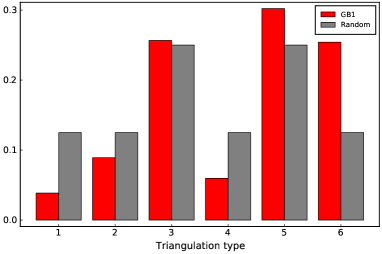
Figure 6: Distribution of triangulation types for 3-locus random fitness landscapes with uniformly distributed fitness (grey bars) and biallelic 3-locus sublandscapes of the GB1 protein fitness landscape of Wu2016 . The probabilities for the random landscapes are close to the simple rationals $\frac{1}{8},\frac{1}{8},\frac{1}{4},\frac{1}{8},\frac{1}{4},\frac{1}{8}$ Srivastava .

Since the present analysis is focused on bi-allelic fitness landscapes, we examined bi-allelic sub-landscapes of the protein landscape. We started from any arbitrary sequence in the genotype space and then considered all the $2^{4}=16$ sequences that can be generated by mutating each locus to a different amino acid. For each locus, there are 19 other possibilities to mutate to, so the number of such sub-landscapes is enormously large. Therefore, we limited our analysis to 10,000 such sub-landscapes. The triangulation imposed by each sub-landscape was computed using the software Macaulay 2. For triangulations that displayed the maximal number of 24 simplices, we checked if the vertices of each of the simplices represented paths from the zero-string 0000 to its antipodal sequence 1111. Upon doing so, we found 10 landscapes that showed the standard staircase triangulation and all of them had either one or two peaks. From this, we can estimate the frequency of any staircase triangulation by multiplying by 8. Thus, we would expect to find around 80 landscapes that show staircase triangulation. Therefore, staircase triangulations are more common in the biological fitness landscape than in random fitness landscapes with completely uncorrelated fitness values.

We additionally determined the distribution over triangulation types of 10,000 3-locus sub-landscapes in the GB1 data and compared this with the corresponding distribution for 10,000 random landscapes (Figure 6). The fraction of GB1 landscapes of types 1, 2 and 4 are reduced in comparison to random landscapes, whereas those of types 3, 4 and 6 are enriched. Out of these, the enrichment of landscapes of type 6 is most notable. The strong over-representation of staircase triangulations in the biological sub-landscapes with 3 and 4 loci confirms the link of positive epistatic interactions to universal positive epistasis and demonstrates the biological relevance of this concept.

4 Circuits, Gröbner bases and the staircase triangulation

A triangulation can be described explicitly by a list of inequalities, or by its minimal non-faces (Chapter 9.4 triangulations ). In brief, let $J$ be a subset of the vertices of the $L$-cube. Then $J$ is a minimally dependent point set if there is an affine dependence relation $\sum_{g\in J}\lambda_{g}g=0$, $\lambda_{v}\in\mathbb{R}$, with $\sum_{g\in J}\lambda_{g}=0$ and $J$ is minimal with this property. The expression $\sum_{g\in J}\lambda_{g}w_{g}$ is called a circuit, or a circuit interaction. A minimal non-face is a set of genotypes that does not belong to any simplex in the triangulation, such that the set is minimal with this property.

One can compare the descriptions for the standard staircase triangulation (Definition 1). The minimal non-faces for $L=3$ are

$\{100,010\},\{100,001\},\{100,011\}$,

$\{010,001\},\{010,101\},\{001,110\}$,

$\{110,011\},\{110,101\},\{101,011\}$.

The triangulation can also be defined by the circuit signs:

$w_{000}+w_{110}-w_{100}-w_{010}>0$

$w_{000}+w_{101}-w_{100}-w_{001}>0$

$w_{000}+w_{011}-w_{010}-w_{001}>0$

$w_{100}+w_{111}-w_{110}-w_{101}>0$

$w_{010}+w_{111}-w_{110}-w_{011}>0$

$w_{001}+w_{111}-w_{101}-w_{011}>0$.

The six circuit signs imply the inequalties:

$w_{111}+w_{000}-w_{110}-w_{001}>0$

$w_{111}+w_{000}-w_{101}-w_{010}>0$

$w_{111}+w_{000}-w_{011}-w_{100}>0$.

The nine inequalities listed correspond exactly to all minimal non-faces (the two rightmost genotypes that appear on each line are the genotypes in the minimal non-faces).

Lemma 2.

The minimal non-faces for the staircase triangulation consist of the sets

$$\{g,g^{\prime}\}\text{ such that }g^{\prime}\not\subset g,g\not\subset g^{\prime}.$$

Proof: Each pair $\{g,g^{\prime}\}$ as above is a minimal non-face. Let $S$ be the set of such pairs. Let $\{g_{1},\dots,g_{r}\}$ be a minimal non-face. The genotypes $g_{1},\dots,g_{r}$ do not all belong to the same simplex, which excludes that the genotypes form a chain $g_{1}\subseteq\dots\subseteq g_{r}.$ It follows that $g_{i}\not\subset g_{j}$ and $g_{j}\not\subset g_{i}$ for some pair $i,j$, and consequently that $\{g_{i},g_{j}\}$ is a non-face. One concludes that $\{g_{1},\dots,g_{r}\}=\{g_{i},g_{j}\},$ which implies that $\{g_{1},\dots,g_{r}\}\in S.$

Observation 8.

If a fitness landscape has universal positive epistasis, then the landscape induces the staircase triangulation.

Proof: It is sufficient to show that the triangulation induced by the fitness landscape has the same minimal non-faces as the staircase triangulation. Let $S$ be the set of pairs

$$\{g,g^{\prime}\}\text{ such that }g^{\prime}\not\subset g,g\not\subset g^{\prime}.$$

By assumption, the landscape has universal positive epistasis so that

$$w_{g\cup g^{\prime}}+w_{g\cap g^{\prime}}\geq w_{g}+w_{g^{\prime}}$$

for any two genotypes $g,g^{\prime}$. If $\{g,g^{\prime}\}\in S$, the inequality is strict. It follows that every element in $S$ is a minimal non-face. Moreover, a non-face of the triangulation cannot consist of genotypes that constitute a chain. By an argument similar to the proof of the previous result, it follows that $S$ is the set of minimal non-faces. Since a landscape with universal positive epistasis has the same minimal non-faces as the staircase triangulation, the result follows.

One can use Gröbner bases froberg for finding all minimal non-faces of a triangulation (Chapter 9.4 triangulations ).

Example 2.

Let $k[x_{00},x_{10},x_{01},x_{11}]$ and $k[x_{0},x_{1},y_{0},y_{1}]$ be polynomial rings, and let $\varphi$ be the map defined by

$$\varphi:\quad\quad x_{00}\mapsto x_{0}y_{0},\quad x_{10}\mapsto x_{1}y_{0}\quad x_{01}\mapsto x_{0}y_{1},\quad x_{11}\mapsto x_{1}y_{1}$$

Let $I={\text{ ker }}\varphi$. Then $I$ is the ideal generated by $x_{11}x_{00}-x_{10}x_{01}$.

Let

$$w=(w_{00},w_{10},w_{01},w_{00})$$

be a weight vector and let $J=in_{-w}(I)$ be the initial ideal with respect to $-w$ (notice the sign here, $-w$ defines the monomial order). If

$$w_{11}+w_{00}-w_{10}-w_{01}>0,$$

then $J=(x_{10}x_{01})$.

According to theory on Gröbner bases and triangulations, the generators of $J$ correspond exactly to the minimal non-faces of the triangulation. One concludes that $\{10,01\}$ is the only minimal non-face and therefore that the triangulation induced by $w$ consists of the simplices $\{00,10,11\}$ and $\{00,01,11\}$.

The following result follows immediately from Sturmfels’ correspondence, see Theorem 9.4.5 in triangulations .

Lemma 3.

Let $k[x_{g}]$ be the polynomial ring in variables labeled by the genotypes $x_{g}$ and let $w$ be the weight vector that defines the fitness landscape. Let $I\subset k[x_{g}]$ be the defining ideal (as in the previous example). If $J=in_{-w}(I)$ is square free, then the generators of $J$ correspond exactly to the minimal non-faces of the triangulation.

The following observations are useful for computational purposes. The results can be deduced from general theory on binomial ideals sturmfelsb . We provide an explicit argument for the readers’ convenience. In addition to the application here (see below) the result should be useful for research on triangulations and peak patterns for higher $L$.

Observation 9.

Let $S$ be the set consisting of all elements of the form

$$x_{g}\cdot x_{g^{\prime}}-x_{g\lor g^{\prime}}\cdot x_{g\wedge g^{\prime}},$$

where $g$ and $g^{\prime}$ are genotypes such that $g^{\prime}\not\subset g$ and $g\not\subset g^{\prime}$. Consider the monomial order defined by a fitness landscape that induces the standard staircase triangulation. With notation as in Example 2, the set $S$ is a Gröbner basis for the defining ideal $I\subset k[x_{g}]$ .

Proof: Let $I$ be the defining ideal and let $J=in_{-w}(I)$. It is easy to verify that $S$ generates $I$. Let $x_{g_{1}}\cdots x_{g_{k}}$ be a generator for $J$. It is sufficient to show that the generator is divisible by a leading term of $S$.

By the previous lemma, the set $\{g_{1},\dots,g_{k}\}$ is a minimal non-face of the triangulation. By Lemma 2,

$$\{g_{1},\dots,g_{k}\}=\{g_{i},g_{j}\}$$

where $g_{i}\not\subset g_{j}$ and $g_{j}\not\subset g_{i}$. By construction, the element

$$x_{g_{i}}x_{g_{j}}-x_{g_{i}\lor g_{j}}\cdot x_{g_{i}\wedge g_{j}}\in S.$$

It follows that $x_{g_{1}}\cdots x_{g_{k}}$ is divisible by $x_{g_{i}}x_{g_{j}}$ and consequently that

$$x_{g_{1}}\cdots x_{g_{k}}=x_{g_{i}}x_{g_{j}}.$$

Observation 10.

For $S$ as defined above, $|S|=2^{L-1}(2^{L}+1)-3^{L}$. By construction, $|S|$ equals the number of minimal non-faces.

Proof: According to Lemma 2, $|S|$ is the number of pairs of genotypes $g,g^{\prime}$ that are neither subsets nor supersets of each other. A genotype $g$ with $k$ 1’s has $2^{k}-1$ subsets and $2^{L-k}-1$ supersets. The number of other genotypes that are neither subsets nor supersets of $g$ is therefore

$$n_{k}=2^{L}-1-(2^{k}-1+2^{L-k}-1)=2^{L}-2^{k}-2^{L-k}+1.$$

Multiplying this with the number of genotypes of size $k$, summing over $k$ and dividing by 2 to avoid overcounting of pairs one arrives at

$$|S|=\frac{1}{2}\sum_{k=1}^{L-1}{L\choose k}n_{k}=2^{L-1}(2^{L}+1)-3^{L}.$$

For $L=4$ the Gröbner basis described above can be given explicitly (see below). The result was applied for verifying that the fitness landscape in Example 1 induces the staircase triangulation.

Gröbner basis for $L=4$:

$x_{1011}\cdot x_{0111}-x_{0011}\cdot x_{1111},\quad x_{1101}\,x_{0111}-x_{0101}\cdot x_{1111}$,

$x_{1110}\cdot x_{0111}-x_{0110}\cdot x_{1111},\quad x_{1101}\cdot x_{1011}-x_{1001}\cdot x_{1111}$,

$x_{1110}\cdot x_{1011}-x_{1010}\cdot x_{1111},\quad x_{1110}\cdot x_{1101}-x_{1100}\cdot x_{1111}$,

$x_{1001}\cdot x_{0111}-x_{0001}\cdot x_{1111},\quad x_{1010}\cdot x_{0111}-x_{0010}\cdot x_{1111}$,

$x_{1100}\cdot x_{0111}-x_{0100}\cdot x_{1111},\quad x_{0101}\cdot x_{1011}-x_{0001}\cdot x_{1111}$,

$x_{0110}\cdot x_{1011}-x_{0010}\cdot x_{1111},\quad x_{1100}\cdot x_{1011}-x_{1000}\cdot x_{1111}$,

$x_{0011}\cdot x_{1101}-x_{0001}\cdot x_{1111},\quad x_{0110}\cdot x_{1101}-x_{0100}\cdot x_{1111}$

$x_{1010}\cdot x_{1101}-x_{1000}\cdot x_{1111},\quad x_{0011}\cdot x_{1110}-x_{0010}\cdot x_{1111}$,

$x_{0101}\cdot x_{1110}-x_{0100}\cdot x_{1111},\quad x_{1001}\cdot x_{1110}-x_{1000}\cdot x_{1111}$,

$x_{1000}\cdot x_{0111}-x_{0000}\cdot x_{1111},\quad x_{0100}\cdot x_{1011}-x_{0000}\cdot x_{1111}$,

$x_{0010}\cdot x_{1101}-x_{0000}\cdot x_{1111},\quad x_{0001}\cdot x_{1110}-x_{0000}\cdot x_{1111}$,

$x_{0101}\cdot x_{0011}-x_{0001}\cdot x_{0111},\quad x_{0110}\cdot x_{0011}-x_{0010}\cdot x_{0111}$,

$x_{1001}\cdot x_{0011}-x_{0001}\cdot x_{1011},\quad x_{1010}\cdot x_{0011}-x_{0010}\cdot x_{1011}$,

$x_{1100}\cdot x_{0011}-x_{0000}\cdot x_{1111},\quad x_{0110}\cdot x_{0101}-x_{0100}\cdot x_{0111}$,

$x_{1001}\cdot x_{0101}-x_{0001}\cdot x_{1101},\quad x_{1010}\cdot x_{0101}-x_{0000}\cdot x_{1111}$,

$x_{1100}\cdot x_{0101}-x_{0100}\cdot x_{1101},\quad x_{1001}\cdot x_{0110}-x_{0000}\cdot x_{1111}$,

$x_{1010}\cdot x_{0110}-x_{0010}\cdot x_{1110},\quad x_{1100}\cdot x_{0110}-x_{0100}\cdot x_{1110}$,

$x_{1010}\cdot x_{1001}-x_{1000}\cdot x_{1011},\quad x_{1100}\cdot x_{1001}-x_{1000}\cdot x_{1101}$,

$x_{1100}\cdot x_{1010}-x_{1000}\cdot x_{1110},\quad x_{0100}\cdot x_{0011}-x_{0000}\cdot x_{0111}$,

$x_{1000}\cdot x_{0011}-x_{0000}\cdot x_{1011},\quad x_{0010}\cdot x_{0101}-x_{0000}\cdot x_{0111}$,

$x_{1000}\cdot x_{0101}-x_{0000}\cdot x_{1101},\quad x_{0001}\cdot x_{0110}-x_{0000}\cdot x_{0111}$

$x_{1000}\cdot x_{0110}-x_{0000}\cdot x_{1110},\quad x_{0010}\cdot x_{1001}-x_{0000}\cdot x_{1011}$,

$x_{0100}\cdot x_{1001}-x_{0000}\cdot x_{1101},\quad x_{0001}\cdot x_{1010}-x_{0000}\cdot x_{1011}$,

$x_{0100}\cdot x_{1010}-x_{0000}\cdot x_{1110},\quad x_{0001}\cdot x_{1100}-x_{0000}\cdot x_{1101}$,

$x_{0010}\cdot x_{1100}-x_{0000}\cdot x_{1110},\quad x_{0010}\cdot x_{0001}-x_{0000}\cdot x_{0011}$

$x_{0100}\cdot x_{0001}-x_{0000}\cdot x_{0101},\quad x_{1000}\cdot x_{0001}-x_{0000}\cdot x_{1001}$,

$x_{0100}\cdot x_{0010}-x_{0000}\cdot x_{0110},\quad x_{1000}\cdot x_{0010}-x_{0000}\cdot x_{1010}$,

$x_{1000}\cdot x_{0100}-x_{0000}\cdot x_{1100}$

Acknowledgments This work was initiated by a mini-symposium at the 2019 SIAM Conference on Applied Algebraic Geometry. We thank Lisa Lamberti for organizing this symposium, for many useful discussions, and for a careful reading of our manuscript. We also thank Muhittin Mungan, Daniel Oros and Anna Seigal for helpful remarks, and two anonymous reviewers for their constructive suggestions.

Notation	Mathematical term	Biological term
$\{0,1\}^{L}$	Bit strings of length $L$	The set of $2^{L}$ genotypes in a biallelic $L$-locus system
$g_{i}$	$i$:th position of the bit string $g$	Locus $i$ of genotype $g$
$g_{i}=1$		$g$ has a 1-allele at locus $i$
$[0,1]^{L}$	Unital $L$-dimensional hypercube	Genotope for a biallelic $L$-locus system (terminology used in the shape theory)
	Vertices with distance $d$ in the undirected cube graph	Genotypes with Hamming distance $d$
	If $d$ (as above) is 1	The genotypes $g$ and $g^{\prime}$ are mutational neighbors
$w:\{0,1\}^{L}\to\mathbb{R}_{\geq 0}\mathchar 24635\relax\;g\mapsto w(g)=w_{g}$		Fitness landscape
	Acyclic directed hypercube graphs induced by fitness landscapes	Fitness graphs: the vertices represent genotypes and edges between mutational neighbors are directed towards genotypes with higher fitness.
	A vertex $g$ is a sink in the fitness graph if all edges incident to $g$ are directed towards $g$.	A genotype $g$ is a peak in the fitness landscape (and fitness graph) if all mutational neighbors of $g$ have strictly lower fitness than $g$.
	The triangulation of $[0,1]^{L}$ induced by the fitness landscape	The shape of the fitness landscape

Table 4: Dictionary of commonly used terms.

References

- \bibcommenthead
- (1) De Visser, J.A.G.M., Krug, J.: Empirical fitness landscapes and the predictability of evolution. Nature Reviews Genetics 15(7), 480–490 (2014)
- (2) Crona, K.: Polytopes, graphs and fitness landscapes. In: Recent Advances in the Theory and Application of Fitness Landscapes, pp. 177–205. Springer, Berlin (2014)
- (3) Domingo, J., Baeza-Centurion, P., Lehner, B.: The causes and consequences of genetic interactions (epistasis). Annual review of genomics and human genetics 20, 433–460 (2019)
- (4) Krug, J.: Epistasis and Evolution. Oxford Bibliographies in Evolutionary Biology, ed. Douglas Futuyama, New York: Oxford University Press, 2021.
- (5) Poelwijk, F.J., Krishna, V., Ranganathan, R.: The context-dependence of mutations: a linkage of formalisms. PLoS computational biology 12(6), 1004771 (2016)
- (6) Beerenwinkel, N., Pachter, L., Sturmfels, B.: Epistasis and shapes of fitness landscapes. Statistica Sinica 17(4), 1317–1342 (2007)
- (7) Crona, K., Greene, D., Barlow, M.: The peaks and geometry of fitness landscapes. Journal of theoretical biology 317, 1–10 (2013)
- (8) de Visser, J.A.G., Park, S.-C., Krug, J.: Exploring the effect of sex on empirical fitness landscapes. The American Naturalist 174(S1), 15–30 (2009)
- (9) De Loera, J., Rambau, J., Santos, F.: Triangulations, Volume 25 of Algorithms and Computation in Mathematics. Springer, Berlin (2010)
- (10) Crona, K., Gavryushkin, A., Greene, D., Beerenwinkel, N.: Inferring genetic interactions from comparative fitness data. Elife 6, 28629 (2017)
- (11) Crona, K., Luo, M., Greene, D.: An uncertainty law for microbial evolution. Journal of theoretical biology 489, 110155 (2020)
- (12) Crona, K.: Rank orders and signed interactions in evolutionary biology. Elife 9, 51004 (2020)
- (13) Das, S.G., Direito, S.O., Waclaw, B., Allen, R.J., Krug, J.: Predictable properties of fitness landscapes induced by adaptational tradeoffs. Elife 9, 55155 (2020)
- (14) Eble, H., Joswig, M., Lamberti, L., Ludington, W.B.: Cluster partitions and fitness landscapes of the drosophila fly microbiome. Journal of mathematical biology 79(3), 861–899 (2019)
- (15) Eble, H., Joswig, M., Lamberti, L., Ludington, W.: Higher-order interactions in fitness landscapes are sparse. arXiv preprint arXiv:2009.12277 (2020)
- (16) Gould, A.L., Zhang, V., Lamberti, L., Jones, E.W., Obadia, B., Korasidis, N., Gavryushkin, A., Carlson, J.M., Beerenwinkel, N., Ludington, W.B.: Microbiome interactions shape host fitness. Proceedings of the National Academy of Sciences 115(51), 11951–11960 (2018)
- (17) Kaznatcheev, A.: Computational complexity as an ultimate constraint on evolution. Genetics 212(1), 245–265 (2019)
- (18) Lienkaemper, C., Lamberti, L., Drain, J., Beerenwinkel, N., Gavryushkin, A.: The geometry of partial fitness orders and an efficient method for detecting genetic interactions. Journal of mathematical biology 77(4), 951–970 (2018)
- (19) Srivastava, M.: Epistasis, shapes and evolution. Master’s thesis, Universität zu Köln (2018). http://kups.ub.uni-koeln.de/id/eprint/9494
- (20) Weinreich, D.M., Watson, R.A., Chao, L.: Perspective: sign epistasis and genetic costraint on evolutionary trajectories. Evolution 59(6), 1165–1174 (2005)
- (21) Poelwijk, F.J., Kiviet, D.J., Weinreich, D.M., Tans, S.J.: Empirical fitness landscapes reveal accessible evolutionary paths. Nature 445(7126), 383–386 (2007)
- (22) Wu, N.C., Dai, L., Olson, C.A., Lloyd-Smith, J.O., Sun, R.: Adaptation in protein fitness landscapes is facilitated by indirect paths. Elife 5, 16965 (2016)
- (23) Herrmann, S., Joswig, M., Speyer, D.E.: Dressians, tropical grassmannians, and their rays. In: Forum Mathematicum, vol. 26, pp. 1853–1881 (2014). De Gruyter
- (24) Pellerin, J., Verhetsel, K., Remacle, J.-F.: There are 174 subdivisions of the hexahedron into tetrahedra. ACM Transactions on Graphics (TOG) 37(6), 1–9 (2018)
- (25) Oros, D.: Hybercubes, peak patterns and universal positive epistasis. Master’s thesis, Universität zu Köln (2022). http://kups.ub.uni-koeln.de/id/eprint/63386
- (26) Huggins, P., Sturmfels, B., Yu, J., Yuster, D.: The hyperdeterminant and triangulations of the 4-cube. Mathematics of Computation 77(263), 1653–1679 (2008)
- (27) Pournin, L.: The flip-graph of the 4-dimensional cube is connected. Discrete & Computational Geometry 49(3), 511–530 (2013)
- (28) Seigal, A., Montúfar, G.: Mixtures and products in two graphical models. Journal of Algebraic Statistics 9, 1–20 (2018)
- (29) Kauffman, S., Levin, S.: Towards a general theory of adaptive walks on rugged landscapes. Journal of theoretical Biology 128(1), 11–45 (1987)
- (30) Macken, C.A., Hagan, P.S., Perelson, A.S.: Evolutionary walks on rugged landscapes. SIAM Journal on Applied Mathematics 51(3), 799–827 (1991)
- (31) Schmiegelt, B., Krug, J.: Evolutionary accessibility of modular fitness landscapes. Journal of Statistical Physics 154(1), 334–355 (2014)
- (32) Haldane, J.B.S.: A mathematical theory of natural selection. part viii: Metastable populations. Mathematical Proceedings of the Cambridge Philosophical Society 27(1), 137–142 (1931)
- (33) Mara, P.S.: Triangulations for the cube. Journal of Combinatorial Theory, Series A 20(2), 170–177 (1976)
- (34) Fröberg, R.: An Introduction to Gröbner Bases. John Wiley & Sons, 111 River Street, Hoboken, NJ 07030-5774, United States (1997)
- (35) Sturmfels, B.: Gröbner Bases and Convex Polytopes vol. 8. American Mathematical Soc., Providence, Rhode Island (1996)