Preparing the next gravitational million-body simulations: Evolution of single and binary stars in Nbody6++GPU, MOCCA and McLuster

Abstract

We present the implementation of updated stellar evolution recipes in the codes Nbody6++GPU, MOCCA and McLuster. We test them through numerical simulations of star clusters containing $1.1\times 10^{5}$ stars (with $2.0\times 10^{4}$ in primordial hard binaries) performing high-resolution direct $N$-body (Nbody6++GPU) and Monte-Carlo (MOCCA) simulations to an age of 10 Gyr. We compare models implementing either delayed or core-collapse supernovae mechanisms, a different mass ratio distribution for binaries, and white dwarf natal kicks enabled/disabled. Compared to Nbody6++GPU, the MOCCA models appear to be denser, with a larger scatter in the remnant masses, and a lower binary fraction on average. The MOCCA models produce more black holes (BHs) and helium white dwarfs (WDs), whilst Nbody6++GPU models are characterised by a much larger amount of WD-WD binaries. The remnant kick velocity and escape speed distributions are similar for the BHs and neutron stars (NSs), and some NSs formed via electron-capture supernovae, accretion-induced collapse or merger-induced collapse escape the cluster in all simulations. The escape speed distributions for the WDs, on the other hand, are very dissimilar. We categorise the stellar evolution recipes available in Nbody6++GPU, MOCCA and Mcluster into four levels: the one implemented in previous Nbody6++GPU and MOCCA versions (level A), state-of-the-art prescriptions (level B), some in a testing phase (level C), and those that will be added in future versions of our codes.

1 Introduction

The stellar environment in star clusters provides the ideal laboratory for investigating stellar binary evolution as well as gravitational wave (GW) physics. This is because the densities are typically so high that stars can interact in close gravitational encounters or even physically collide with each other. These interactions support the presence of more tightly bound binary stars, which can act as a source of huge amounts of gravitational energy to the cluster. This will result in enhanced mass-segregation: more massive stars and binaries sink to the centre of the system, where they undergo close gravitational encounters and in the case of high densities, stellar collisions, which has been predicted and tested theoretically (Heggie, 1975; Portegies Zwart & McMillan, 2002; Khalisi et al., 2007; Giersz et al., 2015; Wang et al., 2016; Askar et al., 2017; Arca Sedda et al., 2019; Rizzuto et al., 2021b; Rizzuto et al., 2021a) and verified observationally (Lada & Lada, 2003; Cantat-Gaudin et al., 2014; Martinazzi et al., 2014; Kamann et al., 2018b; Giesers et al., 2018, 2019).
Simulations of such star clusters fundamentally aim to solve the equations of motion describing $N$ bodies moving under the influence of their own self-gravity. For this purpose a variety of computational approaches have been developed beginning in the first half of the last century. The two main methods in the regime of around $10^{5}-10^{7}$ particles that stand out today are either related to direct $N$-body simulation or Monte-Carlo modelling (Aarseth et al., 1974; Aarseth & Lecar, 1975; Giersz & Heggie, 1994; Spurzem, 1999). Direct $N$-body simulation – orbit integration of the orbits of many particles in a self-gravitating bound star cluster – is the most suitable method to understand relaxation (Larson, 1970a, b) and evolutionary processes in the regime of star clusters. Here, statistical physics still plays a role and more approximate models may be used. These models are based on the Fokker-Planck equation, which can be solved either directly or by a Monte Carlo Markoff chain method (Hénon, 1975; Cohn, 1979; Stodolkiewicz, 1982, 1986; Giersz, 1998; Giersz et al., 2015; Merritt, 2015; Askar et al., 2017; Kremer et al., 2020a, 2021).
Beyond solving the equations of motion for the $N$ bodies, the complete description of a realistic star cluster becomes much more complicated, because the stellar evolution of single and binary stars has an enormous impact on the dynamical evolution of star clusters. Single and binary stars may suffer significant mass loss over the lifetime of the cluster depending on their initial zero-age main sequence (ZAMS) mass and their metallicity. This mass loss changes the potential of the star cluster and subsequently has an effect on the orbits of the stars. In our models of single stars, this mass loss is dominated by stellar winds and outflows (Hurley et al., 2000; Tout, 2008a). In the models of binary stars, the member stars can interact with each other closely and other astrophysical processes involving dynamical mass transfer, tidal circularisation and stellar spin synchronisation happen (Mardling & Aarseth, 2001; Hurley et al., 2002; Tout, 2008b). In the case of compact objects like black holes (BHs), neutron stars (NSs), and white dwarfs (WDs) repeated encounters between stars and binaries may lead to sudden orbit shrinking of a binary up to a point when finally a huge proportion of further orbit shrinking is due to the emission of gravitational radiation (Faye et al., 2006; Brem et al., 2013; Antonini & Gieles, 2020; Arca Sedda et al., 2020; Mapelli et al., 2020a). The gravitational waves that accompany these subsequent gravitational inspiral events might be detectable with the (Advanced) Laser Interferometer Gravitational-Wave Observatory (aLIGO) (Aasi et al., 2015; Abbott et al., 2018; Abbott et al., 2019), (Advanced) Virgo Interferometer (aVirgo) (Acernese et al., 2015; Abbott et al., 2018; Abbott et al., 2019) if they emit signals coming from merging NSs (Abbott et al., 2017a, b), stellar mass BHs (Abbott et al., 2016) or the process of core collapse in supernovae (SNe) (Ott, 2009). If, for example, the binary consists of two BHs then this gravitational wave inspiral may lead to the formation of intermediate-mass BHs (IMBHs) as has been confirmed in simulations (Giersz et al., 2014, 2015; Arca Sedda et al., 2019; Rizzuto et al., 2021b; Di Carlo et al., 2019; Di Carlo et al., 2020a; Di Carlo et al., 2020b, 2021; Banerjee, 2021b, a). A recent aLIGO and aVirgo detection of such an IMBH with a total mass of around 142 $\mathrm{M}_{\odot}$ (Abbott et al., 2020a) invites further simulations focussing on this particular aspect.
A subclass of star clusters that we aim to simulate across cosmic time are globular clusters (GCs). The Milky way hosts over 150 of these (Harris, 1996; Baumgardt & Hilker, 2018). Their old age and relatively large numbers not only in our galaxy, but also in much more massive elliptical galaxies such as M87 (Tamura et al., 2006b, a; Doyle et al., 2019), and at higher redshifts (Zick et al., 2018a; Zick et al., 2018b; Zick et al., 2020) all suggest that they play an important role as a fundamental building block in a hierarchy of cosmic structure formation (Reina-Campos et al., 2019; Reina-Campos et al., 2020, 2021). Although becoming increasingly sophisticated, observational studies using astrophysical instruments such as Multi Unit Spectroscopic Explorer (MUSE) (Husser et al., 2016; Giesers et al., 2018, 2019; Kamann et al., 2018a, b, 2020a, 2020b) and Gaia (Kuhn et al., 2019; Bianchini et al., 2013; Bianchini et al., 2018, 2019; de Boer et al., 2019; Huang & Koposov, 2021) are not sufficient on their own to resolve the complete evolution of GCs across cosmic time, because they effectively only take snapshots of these clusters today. These observations must therefore be supplemented with astrophysical simulations (Krumholz et al., 2019). Due to their typical sizes, simulations of GCs over billions of years are at the edge of high-resolution direct $N$-body simulations today, which are computationally possible and feasible. The Dragon simulations were the first, and last to date, direct gravitational million-body simulations of such a GC (Wang et al., 2016). Similarly, the last direct million-body simulation of a nuclear star cluster (NSC) (similar particle number as the Dragon simulations, but scaled in a way to resemble a NSC) harbouring a central and accreting SMBH were performed by Panamarev et al. (2019). While Wang et al. (2015) made the technical programming advances necessary to perform million-body simulations with Nbody6++GPU in the first place by parallelising the integrations across multiple GPUs accelerating the (regular) direct force integrations and the energy checks to an unprecedented degree and while Panamarev et al. (2019) expanded the code to include a central and accreting SMBH, the stellar evolution prescriptions in both of these codes were largely unchanged.
To this end, we updated the stellar evolution routines in the direct-force integration code Nbody6++GPU (Wang et al., 2015), which are the SSE (Hurley et al., 2000) and BSE (Hurley et al., 2002) stellar evolution implementations. These updates mirror the updates in Nbody7 by Banerjee et al. (2020); Banerjee (2021b). The results are then compared with the Hénon-type Monte-Carlo code MOCCA (Hypki & Giersz, 2013; Giersz et al., 2013), which also conveniently models the evolution of single and binary stars with the SSE and BSE routines. This study is therefore also a continuation of the productive collaboration between the teams surrounding these modelling methods (Giersz et al., 2008; Downing et al., 2010, 2011; Giersz et al., 2013; Wang et al., 2016; Rizzuto et al., 2021b). Finally, in the appendix, we present an updated version of McLuster (Kuepper et al., 2011), which now includes a mirror of the stellar evolution available in Nbody6++GPU.

2 Methods

2.1 Direct $N$-body simulations with Nbody6++GPU

The state-of-the-art direct force integration code Nbody6++GPU is optimised for high performance GPU-accelerated supercomputing (Spurzem, 1999; Nitadori & Aarseth, 2012; Wang et al., 2015). This code follows a long-standing tradition in a family of direct force integration codes of gravitational $N$-body problems, which were originally written by Sverre Aarseth (Aarseth (1985); Spurzem (1999); Aarseth (1999a, b, 2003); Aarseth et al. (2008) and sources therein) and now spans a more than 50 year-long history of development. The afore-mentioned code Nbody7 (Aarseth, 2012) also stems from this family, but it is its own serial code using the algorithmic regularization chain method (Mikkola & Aarseth, 1993; Mikkola & Tanikawa, 1999a, b; Mikkola & Merritt, 2008; Hellström & Mikkola, 2010). It is not optimised for massively parallel supercomputers, unlike Nbody6++GPU, which is currently one of the best available high accuracy, massively parallel, direct $N$-body simulation codes. Two very promising alternative and supposedly faster codes have been published during the preparation of this paper; the PeTar (Wang et al., 2020a, b; Wang et al., 2020c) and FROST/MSTAR (Rantala et al., 2020; Rantala et al., 2021) codes. These two codes are more recently developed and less mature.
The Dragon simulations performed with Nbody6++GPU by Wang et al. (2016) are currently still the world-record holder for the largest and most realistic star cluster simulations. The code is optimised for large-scale computing clusters by utilising MPI (Spurzem, 1999), OpenMP and GPU (Nitadori & Aarseth, 2012; Wang et al., 2015) parallelisation techniques. In combination with intricate and highly sophisticated algorithms, such as the Kustaanheimo-Stiefel (KS) regularisation (Stiefel & Kustaanheimo, 1965), the Hermite scheme with hierarchical block time-steps (McMillan, 1986; Hut et al., 1995; Makino, 1991, 1999) and the Ahmad-Cohen (AC) neighbour scheme (Ahmad & Cohen, 1973), the code thus allows for star cluster simulations of realistic size without sacrificing astrophysical accuracy by not properly resolving close binary and/or higher-order subsystems of (degenerate) stars. With Nbody6++GPU we can include hard binaries and close encounters (binding energy comparable or larger than the thermal energy of surrounding stars) using two-body and chain regularization (Mikkola & Tanikawa, 1999a, b; Mikkola & Aarseth, 1998), which permits the treatment of binaries with periods of days in conjunction and multi-scale coupling with the cluster environment. The AC scheme permits for every star to divide the gravitational forces acting on it into the regular component, originating from distant stars, and an irregular part, originating from nearby stars (“neighbours”). Regular forces, efficiently accelerated on the GPU, are updated in larger regular time steps, while neighbour forces are much more fluctuating and need update in much shorter time intervals. Since neighbour numbers are usually small compared to the total particle number, their implementation on the CPU using OpenMP (Wang et al., 2015) provides the best overall performance. Post-Newtonian dynamics of relativistic binaries is currently still using the orbit-averaged Peters & Matthews formalism (Peters & Mathews, 1963; Peters, 1964), as described e.g. in Di Carlo et al. (2019); Di Carlo et al. (2020a); Di Carlo et al. (2020b, 2021); Rizzuto et al. (2021b); Rizzuto et al. (2021a); Arca-Sedda et al. (2021). In those papers a collisional build-up of massive black holes, over one or even several generations of mergers, was found. The final merger of two massive black holes seen in the simulations is comparable to the most massive one observed by LIGO/Virgo (Abbott et al., 2020a).

There is an experimental version of the Nbody6++GPU code available on request, which uses a full post-Newtonian dynamics up to order PN3.5 including spins of compact objects, spin-orbit coupling to next-to-lowest order and spin-spin coupling to lowest order (Blanchet, 2014). It will provide more accurate orbital evolution and better predictions for gravitational waveforms in the final phases before coalescence. An early version of this code variant (only up to PN2.5) has been published in Kupi et al. (2006); Brem et al. (2013).

2.2 Monte-Carlo modelling with MOCCA

For modelling star clusters there are Monte Carlo methods available that statistically solve the Fokker-Planck equation, which describes gravitational N-body systems (Hénon, 1975). This method is computationally much less taxing than direct $N$-body (Giersz et al., 2008; Downing, 2012; Hypki & Giersz, 2013; Giersz et al., 2013), but that comes at a cost. It is less realistic in the sense that it can only describe spherical systems. This means that rotation cannot be implemented in these Monte Carlo simulations unlike direct $N$-body simulations (Einsel & Spurzem, 1999; Spurzem, 2001; Ernst et al., 2007; Kim et al., 2008; Amaro-Seoane et al., 2010; Fiestas & Spurzem, 2010; Hong et al., 2013). This assumption means that MOCCA, for example, cannot investigate tidal tails (Baumgardt & Makino, 2003; Madrid et al., 2017). For the Monte-Carlo models of star cluster simulations in this paper we use the MOnte Carlo Cluster SimulAtor MOCCA (Hypki & Giersz, 2013; Giersz et al., 2013). This code is based on an improvement of the original Hénon-type Monte-Carlo Fokker-Planck method by Stodolkiewicz (1982, 1986) and in a further iteration by Giersz (1998, 2001) and ultimately by Giersz et al. (2013). This approach combines the statistical treatment of the process of relaxation with the particle based approach of direct $N$-body simulations. With this, they are able to model spherically symmetric star clusters over long dynamical times. Three- and four-body interactions in the star cluster simulation are computed separately by the FEWBODY code (Fregeau et al., 2004). Furthermore, the escapers from tidally limited star clusters are described by Fukushige & Heggie (2000). Here, the escaping stars stay in the system for some time depending on the excess energy above the escape energy.
The MOCCA Survey Database I (Askar et al., 2017), which provides a grid of about 2000 GC models, something that is currently unthinkable with direct $N$-body simulations, is a major outcome of the work with MOCCA and is also a testament to the strengths of this modelling approach, which has led to a large number of subsequent studies (Morawski et al., 2018, 2019; Arca Sedda et al., 2019; Hong et al., 2020b, 2018, a; Leveque et al., 2021). With this database, we can choose appropriate initial conditions for realistic star cluster simulations using direct $N$-body methods. It is important to stress, that despite some important physical simplification of the Monte Carlo method, the results of the MOCCA simulations agree very well with the results of $N$-body simulations for clusters with different initial number of stars (from $10^{4}$ up to $10^{6}$) and evolving in different host environments (Giersz et al., 2013, 2016; Heggie & Giersz, 2014; Wang et al., 2016; Madrid et al., 2017). The agreement is not only good for the cluster global properties, but also for properties of the binary population (Geller et al., 2019; Rizzuto et al., 2021b).

2.3 Summary: stellar evolution updates (SSE & BSE) in NBODY6++GPU and MOCCA

In this paper we present updates in the SSE & BSE routines in the two codes Nbody6++GPU & MOCCA. The details of these updates are shown in Tab.4 and Tab.5, respectively. These updates make MOCCA & Nbody6++GPU largely competitive in their stellar evolution with other codes that are used to simulate star clusters, such as the Monte-Carlo code CMC (Kremer et al., 2018, 2019, 2020a) with the COSMIC implementation (Breivik et al., 2020) or the new, massively parallel direct $N$-body code PeTar (Wang et al., 2020b). Furthermore, we are now in a position to model the full evolution of aLIGO/aVirgo gravitational wave sources and their progenitor stars up until the eventual merger according to our best current theoretical understanding. We also implemented the SSE & BSE version that is shown in Tab.4 into our version of McLuster and we are now able to produce initial star cluster models that have proper evolution of multiple stellar populations (this will be elaborated in a further publication). The details are shown in Appendix B, where also two use-cases are demonstrated to confirm excellent agreement with the SSE & BSE updates in Nbody7 and the results in Banerjee et al. (2020); Banerjee (2021b).
The SSE & BSE implementation within our versions of Nbody6++GPU, MOCCA & McLuster all contain:

• updated metallicity dependent stellar winds (Vink et al., 2001; Vink & de Koter, 2002, 2005; Belczynski et al., 2010),

• updated metallicity dependent core-collapse SNe, their remnant masses and fallback (Fryer et al., 2012; Banerjee et al., 2020),

• updated electron-capture supernovae (ECSNe), accretion-induced collapse (AIC) and merger-induced collapse (MIC) remnant masses and natal kicks (Nomoto, 1984, 1987; Nomoto & Kondo, 1991; Saio & Nomoto, 1985, 2004; Kiel et al., 2008; Gessner & Janka, 2018)

• (P)PISNe remnant masses (Belczynski et al., 2010, 2016; Woosley, 2017),

• updated fallback-scaled natal kicks for NSs and BHs (Fuller et al., 2003; Scheck et al., 2004; Fryer, 2004; Fryer & Kusenko, 2006; Meakin & Arnett, 2006, 2007; Fryer & Young, 2007; Scheck et al., 2008; Fryer et al., 2012; Banerjee et al., 2020),

• and BH natal spins (see also Belczynski et al. (2020); Belczynski & Banerjee (2020)) from

  • Geneva model (Eggenberger et al., 2008; Ekström et al., 2012; Belczynski et al., 2020; Banerjee, 2021b),

  • MESA model (Spruit, 2002; Paxton et al., 2011, 2015; Belczynski et al., 2020; Banerjee, 2021b),

  • and the Fuller model (Fuller & Ma, 2019; Fuller et al., 2019; Banerjee, 2021b).

The SSE & BSE implementation within MOCCA contains, on top of the above:

• winds by Giacobbo et al. (2018),

• winds depending on surface gravity and effective temperature of a star by Schröder & Cuntz (2005),

• (P)PISNe from SEVN simulations by Spera & Mapelli (2017),

• an earlier treatment by Tanikawa et al. (2020) to model the evolution of extremely metal-poor and high mass POP III stars,

• and proper CV treatment and related dynamical mass transfer, magnetric braking and gravitational radiation critera by Belloni et al. (2018b).

The SSE & BSE algorithms of Nbody6++GPU and McLuster contain, on top of the list of the commonalities between the three codes:

• moderate and weak (P)PISNe by Leung et al. (2019b),

• and WD kicks from Fellhauer et al. (2003).

We discuss future updates in section 5.2.

3 Initial models - delayedSNe-Uniform & rapidSNe-Sana

Parameter	Nbody6++GPU & MOCCA
Particle number	110000
Binary fraction $f_{\text{fb}}$	$10.0\%$
Half mass radius $r_{\text{h}}$	$1.85$ pc
Tidal radius $r_{\text{tid}}$	$500$ pc
IMF	Kroupa IMF, ($0.08-100$) $\text{M}_{\odot}$
Metallicity $Z$	$0.00051$
Density model	King model, $w_{0}=3.0$
Eccentricity distribution	Thermal
Semi-major axis distribution	flat in log

Table 1: Initial models for the (MOCCA & Nbody6++GPU) simulations.

We choose two initial models, which we generate with McLuster (Kuepper et al., 2011), that satisfy the following conditions. Firstly, we do not want these models to be too dense, as we prefer that the dynamics does not overly interfere with the stellar evolution in the star cluster pre-core collapse evolution and secondly, we want the models to have a large tidal radius in order to curtail initial mass loss from the cluster models. With this, we arrive at the structural parameters listed in Tab.1. We have a total number of $1.1\times 10^{5}$ particles (i.e. stars), of which $2.0\times 10^{4}$ are initially in primordial hard binaries. The number of binaries is thus $1.0\times 10^{4}$ and the binary fraction is $f_{\rm b}=10$% The initial half-mass radius $r_{\text{h,0}}$ is set to $1.85$ pc. The smaller particle number then introduces the problem of enhanced mass loss from the cluster. We therefore put the cluster on a circular orbit with a galacto-centric distance of $259.84$ kpc in a MW-like point mass potential of $2.92\times 10^{12}$ $\mathrm{M}_{\odot}$. This gives an initial tidal radius $r_{\text{tid,0}}$ of $500$ pc in order to curtail this initial mass loss. The density model is a King model with a concentration parameter with $w_{0}=3.0$ (King, 1966) and since it is extremely tidally underfilling, it is very close to the corresponding isolated model. The metallicity of the cluster is set to a low, but realistic (metallicity of the GC NGC3201 (Harris, 1996)) value of $Z=0.00051$, meaning that 0.051 per cent of the mass in the cluster stars is not hydrogen or helium. The IMF is set in a range from ($0.08$-$100.0$) $\mathrm{M}_{\odot}$, following Kroupa (2001).
The binaries are initially thermally distributed in their eccentricities as is the current standard in $N$-body simulations (Kroupa, 2008). This, in general, may overpredict the merger rates significantly (Geller et al., 2019). The binary semi-major axes follow flat distributions in the logarithm of the semi-major axis. The minimum and maximum of the semi-major axes distributions of the primordial binary population are set to the radius of the lowest mass star in the star cluster and $100$ AU, respectively. This distribution of binary semi-major axes for hard binaries is reproduced from an initial distribution that includes many more, wider binaries initially in Kroupa (1995b).
The difference between the two distinct initial models that we use in this work arises from the choice of binary mass-ratio distribution and SN mechanism. For one model we use the uniform binary mass-ratio distribution $q_{\mathrm{Uniform}}$ and the delayed SNe mechanism and for the other we use the Sana binary mass-ratio distribution $q_{\mathrm{Sana}}$ (Kiminki et al., 2012; Sana & Evans, 2011; Sana et al., 2013; Kobulnicky et al., 2014) along with activating the rapid SNe treatment (Fryer et al., 2012) (both Level B: the parameters chosen are highlighted in orange in Tab.3, 4 and 5). To clarify, in the $q_{\mathrm{Sana}}$ mass ratio distribution, all the stars that have a mass above 5.0 $\mathrm{M}_{\odot}$ get paired with a secondary, such that the mass ratios are uniformly distributed in the range of $0.1\leq q\leq 1.0$. The rest of the stars are paired randomly in their mass ratios. In this way, $q_{\mathrm{Sana}}$ and $q_{\mathrm{Uniform}}$ are actually quite similar in theory and we will find out if this is case through the simulations over time. An important point is that through the pairing algorithm for $q_{\mathrm{Sana}}$ in McLuster (with pairing=3), we first select all stars and after that we pair them, so we strictly speaking do respect the IMF (Oh et al., 2015).
These two separate models will be referred to as delayedSNe-Uniform and rapidSNe-Sana henceforth. In all other respects the stellar evolution settings of the two simulations are identical (Level B). The stellar evolution levels and their definitions may be understood from Tab.3, Tab.4 (Nbody6++GPU settings) and Tab.5 (MOCCA settings).
We do not enable any (P)PISNe schemes (parameters psflag, piflag) for the Nbody and MOCCA simulations due to the maximum of the IMF at $100\mathrm{M}_{\odot}$ and the low initial cluster density (because of models with very low central density are expected only a few expected stellar mergers that produce stellar masses large enough to be progenitors of (P)PISNe BHs, compare Kremer et al. (2020b)). Furthermore, the Nbody6++GPU models have the WD natal kicks switched on following Fellhauer et al. (2003) and the MOCCA simulations do not assign natal kicks to the WDs. Moreover, the winds in the MOCCA simulations with edd_factor=0 ignore the so-called bi-stability jump (see Appendix A2), whereas the Nbody6++GPU simulations with mdflag=3 do not ignore it (Belczynski et al., 2010).

Following the original concept in Hurley et al. (2002), we define time step parameters $p_{1},p_{2},p_{3}$, to determine how many steps are done during certain evolutionary phases of stars (Note that Banerjee et al. (2020) use symbols pts1, pts2 & pts3 for these). Also MOCCA uses via BSE the same representation. $p_{1}$ describes the step used in the main sequence phase, $p_{2}$ in the sub-giant (BGB) and Helium main sequence phase, and $p_{3}$ in more evolved giant, supergiant, and AGB phases. For clarity we reproduce the equation in Hurley et al. (2002), where $\delta t_{k}$ is the time step used to update the stellar evolution in the code, for stellar type $k$:

$$\delta t_{k}=p_{k}\begin{cases}t_{\rm MS}&k=0,1\\ (t_{\rm BGB}-t_{\rm MS})&k=2\\ (t_{\rm inf,1}-t)&k=3\,t\leq t_{x}\\ (t_{\rm inf,2}-t)&k=3\,t>t_{x}\\ t_{\rm He}&k=4\\ (t_{\rm inf,1}-t)&k=5,6\,t\leq t_{x}\\ (t_{\rm inf,2}-t)&k=5,6\,t>t_{x}\\ t_{\rm HeMS}&k=7\\ (t_{\rm inf,1}-t)&k=8,9\,t\leq t_{x}\\ (t_{\rm inf,2}-t)&k=8,9\,t>t_{x}\\ \max(0.1,10.0t)&k\geq 10\end{cases}$$ (1)

The original choice in Hurley et al. (2000) was $p_{0,1}=0.01$, $p_{2,7}=0.05$, and $p_{k}=0.02$ for all other $k$. During the following years, in widely used Nbody6 codes and derivatives, and in standard BSE packages $p_{0,1}$ and $p_{4}$ have been increased to 0.05, probably to save some computing time. However, after comparison with Startrack (Belczynski et al., 2008) models with high time resolution, Banerjee et al. (2020) suggested $p_{0,1}=0.001$, $p_{2}=0.01$ and $p_{k}=0.02$ for all others. In Fig.4 in Banerjee et al. (2020), we can see the difference that these time-step choices produce, by producing spikes in the initial-final mass relation for large progenitor ZAMS masses (ignoring (P)PISNe). Currently such small $p_{i}$ does not pose any significant computational problem; but as seen in Banerjee et al. (2020) such problems with too large $p_{i}$ only show up for very large stellar masses $M\gtrsim 100\text{M}_{\odot}$.

4 Results

4.1 Global dynamical evolution

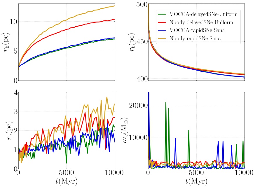
Figure 1: Time evolution of the half-mass radii $r_{\mathrm{h}}$(pc) (top-left), the tidal radii $r_{\mathrm{t}}$(pc) (top-right), core radii $r_{\mathrm{c}}$(pc) (bottom-left) and core masses $m_{c}$($\text{M}_{\odot}$) (bottom-right) for the four simulations. The Nbody-delayedSNe-Uniform, Nbody-rapidSNe-Sana, MOCCA-delayedSNe-Uniform and MOCCA-rapidSNe-Sana simulations are shown in red, yellow, green and blue, respectively.

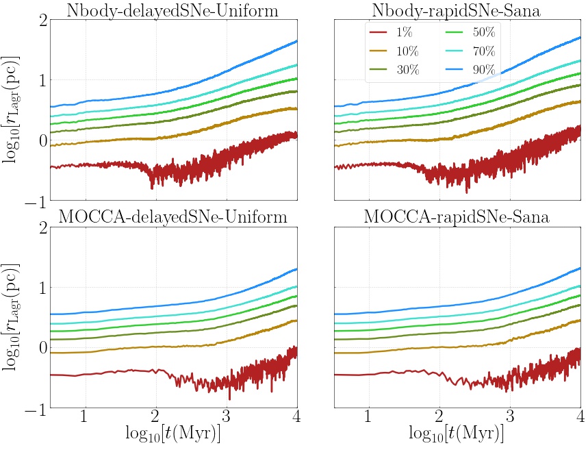
Figure 2: Time evolution of the logarithm of the Lagrangian radii $r_{\mathrm{Lagr}}$ $(1,10,30,50,70,90)$% for the four simulations: Nbody-delayedSNe-Uniform (top-left), Nbody-rapidSNe-Sana (top-right), MOCCA-delayedSNe-Uniform (bottom-left) and MOCCA-rapidSNe-Sana (bottom-right).

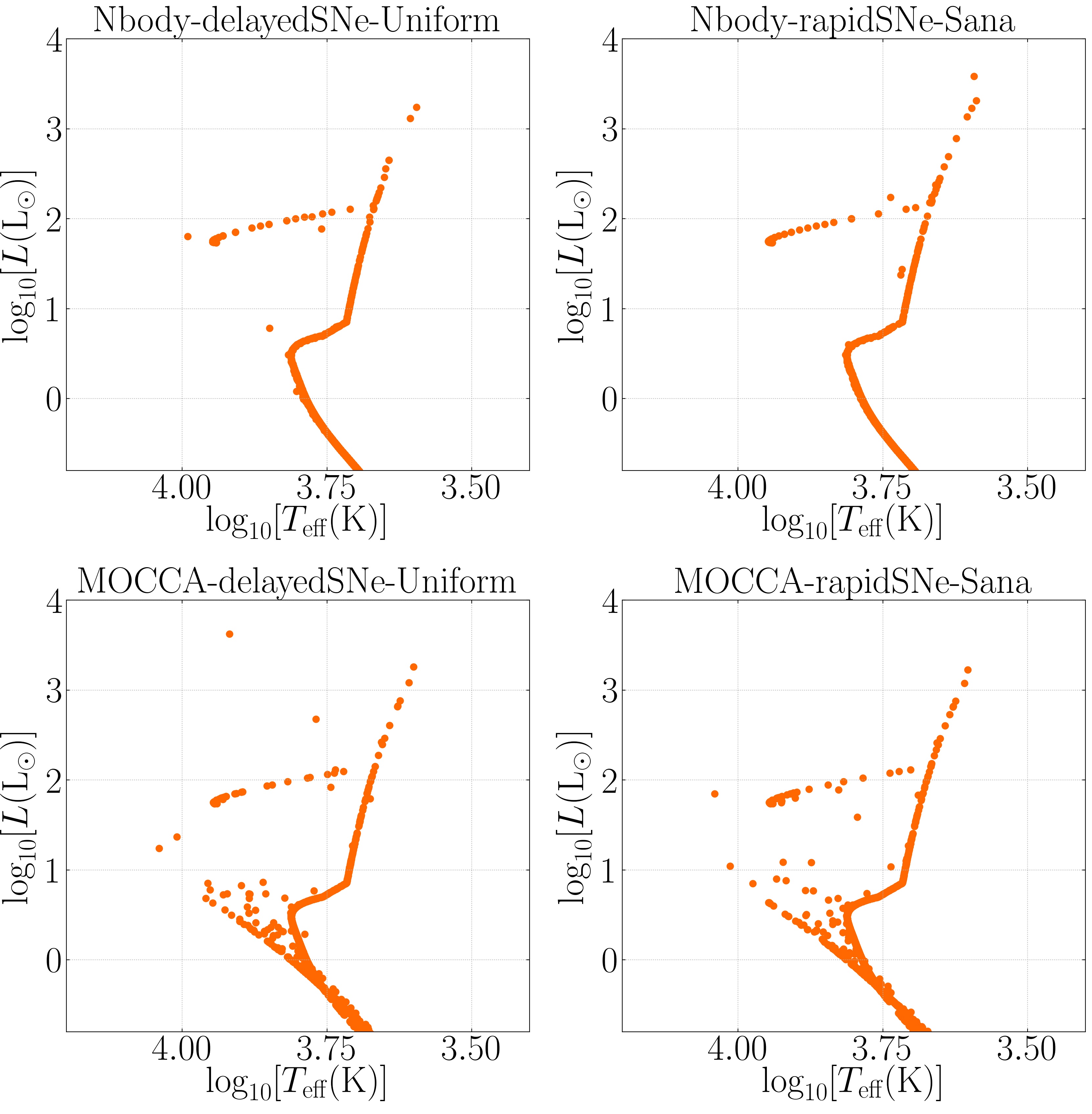
Figure 3: HRD for all four simulates at 10 Gyr. As can be seen from the HRDs of the MOCCA simulations, there are plenty of more blue stragglers in these than in the Nbody6++GPU simulations.

We run each of the two initial models with Nbody6++GPU and MOCCA. Hence we have four distinct simulations to compare and contrast. We discuss in the following Figs. 1 to 3, to get an overview over the global evolution of the simulated star clusters.

Fig.2 shows us that the core collapse happens a bit later in the MOCCA simulations and this is connected with the problems with the timescale. According to Hênon’s principle, the rate of cluster evolution is governed by the heat flow through the half-mass radius. Therefore, for smaller $r_{\mathrm{h}}$ and half-mass relaxation time, $t_{\mathrm{h}}$, in MOCCA than in the Nbody6++GPU models, the MOCCA models have to evolve faster and provide more energy in the core than their Nbody6++GPU counterparts. This leads to more dynamical interactions in the core and a small delay in the core-collapse time. Primordial binaries become active earlier as an energy source than in the direct $N$-body simulations. This can also be seen from the core radii, $r_{\mathrm{c}}$, evolution of the cluster models and we see that the MOCCA simulations have a larger central density, which should lead to a larger number of dynamical interactions in MOCCA compared with the Nbody6++GPU runs. Likewise, this can be observed in the larger scatter in remnant masses in Fig.6. In combination with the smaller $r_{\mathrm{h}}$ in the MOCCA models, which have a similar total mass (similar $r_{\mathrm{t}}$ in all) to those of the Nbody6++GPU models, this means that the energy flow across $r_{\mathrm{h}}$ is much larger in MOCCA than in the Nbody6++GPU runs. The denser models in the MOCCA simulations are evidenced further in the number of binaries in the simulations. The time evolution of the logarithm of the binary fraction for the four simulations is shown in the top-row of Fig.4. Although the overall binary fractions are similar, the Nbody6++GPU simulations yield consistently larger fractions over 10 Gyr. This is due to more scattering events in MOCCA runs that disrupt binaries, which is mirrored by the denser cores and overall clusters in the MOCCA simulations, see Fig.1. Moreover, looking at Fig.6, one can see from the larger scattering in the remnant masses of all compact objects in the MOCCA simulations that there must have been more interactions between the stars that led to mass gain or loss. This is further evidenced by the Hertzsprung-Russel diagram (HRD) in Fig.3 from all four simulations. We see many more blue stragglers in the HRDs of MOCCA compared with the Nbody6++GPU simulations. This means that there must have been collisions or mass transfer to rejuvenate the stars in order to make them blue stragglers. The likelihood of these formation channels is generally larger in denser systems.

4.2 Stellar evolution

4.2.1 Compact binary fractions

Fig.4 shows, in addition to the overall binary fraction, the binary fractions of several other compact binaries in which at least one member is a compact object. Both compact binary fractions are dominated by WD binaries, where in the MOCCA simulations the WD binaries are mostly found as WD-MS binaries. In the Nbody6++GPU simulations, there also many WD binaries consisting of secondaries other than MSs, many of them also being WDs. In all simulations the overall WD binary fraction, as well as the WD-MS binary fraction increases over the whole 10 Gyr in contrast to the total star cluster binary fraction. The double-degenerate (DD) binary fraction for all simulations also increases continuously. This is dominated by WD-WD binaries, where the number of surviving WD-WD binaries in the Nbody6++GPU simulations is much larger than the number in the MOCCA simulations by a factor of about ten. This large discrepancy could be due to faster evolving and denser MOCCA star cluster simulations, which ionise or force to merge more binaries. This is also evidenced by the lower overall binary fractions in the MOCCA models: see also the discussion above.
Further differences in WD binary fractions, especially the WD-MS binaries in Fig.4, might additionally arise from the WD kicks that are switched on in the Nbody6++GPU simulations but not in the MOCCA models. In general, these WD kicks are the same for WD types in MOCCA and are assigned an arbitrary kick speed of vkickwd, unlike in Nbody6++GPU, which draws kicks for HeWDs and COWDs from a Maxwellian of dispersion wdksig1 and the kicks for the ONeWDs from a Maxwellian with dispersion wdksig2. Both Maxwellians are truncated at wdkmax=6.0 $\text{kms}^{-1}$, where typically wdksig1=wdksig2=2.0 $\text{kms}^{-1}$ following (Fellhauer et al., 2003). The presence of these kicks in the Nbody6++GPU models might lead to increased disruption of WD-MS binaries and thus lead to the observed lower abundances. However, since MOCCA and Nbody6++GPU lead to faster and slower global evolution of the star cluster models, respectively, it is difficult to disentangle what actually produces these differences. So far, no cluster simulations on the scale of our simulations presented here have been undertaken investigating the stability of WD binaries in the presence of kicks in detail using both MOCCA and Nbody6++GPU and these need to be performed in the future.
From Fig.4 we can see that near the beginning of all simulations there are small numbers of BH-MS binaries produced for all four simulations, where the delayedSNe-Uniform simulations produce more BH-MS binaries overall. Over the 10 Gyr evolution of our cluster simulations, the MOCCA-delayedSNe-Uniform simulation produces the most surviving BH-MS binaries, but the logarithmic binary fraction is still continuously decreasing. All simulations produce BH-BH binaries in similar numbers where these start forming after about 100 Myr. This suggests that BH-BH binary systems formed in dynamic interactions, since the last BH formed in a SNe was about 80 Myr earlier. At the end of all simulations, we have a surviving BH-BH, whose orbital parameters and masses may be inspected in Tab.2. All of these binaries are located very close to the cluster density centre, with masses of the same order of magnitude, with the highest mass BH in a BH-BH (and all BH binaries) being found in the MOCCA-rapidSNe-Sana model with mass $M_{\mathrm{BH}}=31.032$ $\mathrm{M}_{\odot}$. The semi-major axes $a$ of these BH-BH binaries are also all smaller than $100$ AU: the closest BH-BH binary found in the Nbody-delayedSNe-Uniform simulation having a semi-major axis value of $53.129$ AU. This is not small enough to have a merger within a Hubble time. The two BH-MS binaries in the MOCCA-delayedSNe-Uniform simulation both consist of an accreting BH with a low mass MS donor star of type KW=0. Therefore, these are not given in Tab.2.
The NS binaries are found further away from the density centre, the closest one coming from the MOCCA-delayedSNe-Uniform run with $r_{\mathrm{dens}}=2.018$ pc. The simulations do not produce any surviving NS-NS, NS-BH, or BH-WD binaries, the former of which are very elusive (Arca Sedda, 2020; Chattopadhyay et al., 2020; Chattopadhyay et al., 2021; Drozda et al., 2020). The MOCCA-rapidSNe-Sana simulation produces one surviving BH-MS binary, whose parameters are given in Tab.2. All simulations produce NS binaries, where at 10 Gyr we have mostly only NS-MS binaries surviving, apart from the Nbody6++GPU-delayedSNe-Uniform simulation, which also produces one NS-COWD binary: see Tab.2. All NS masses in binaries are 1.26 $\mathrm{M}_{\odot}$ and thus these are either the result of a MIC, AIC or ECSNe.

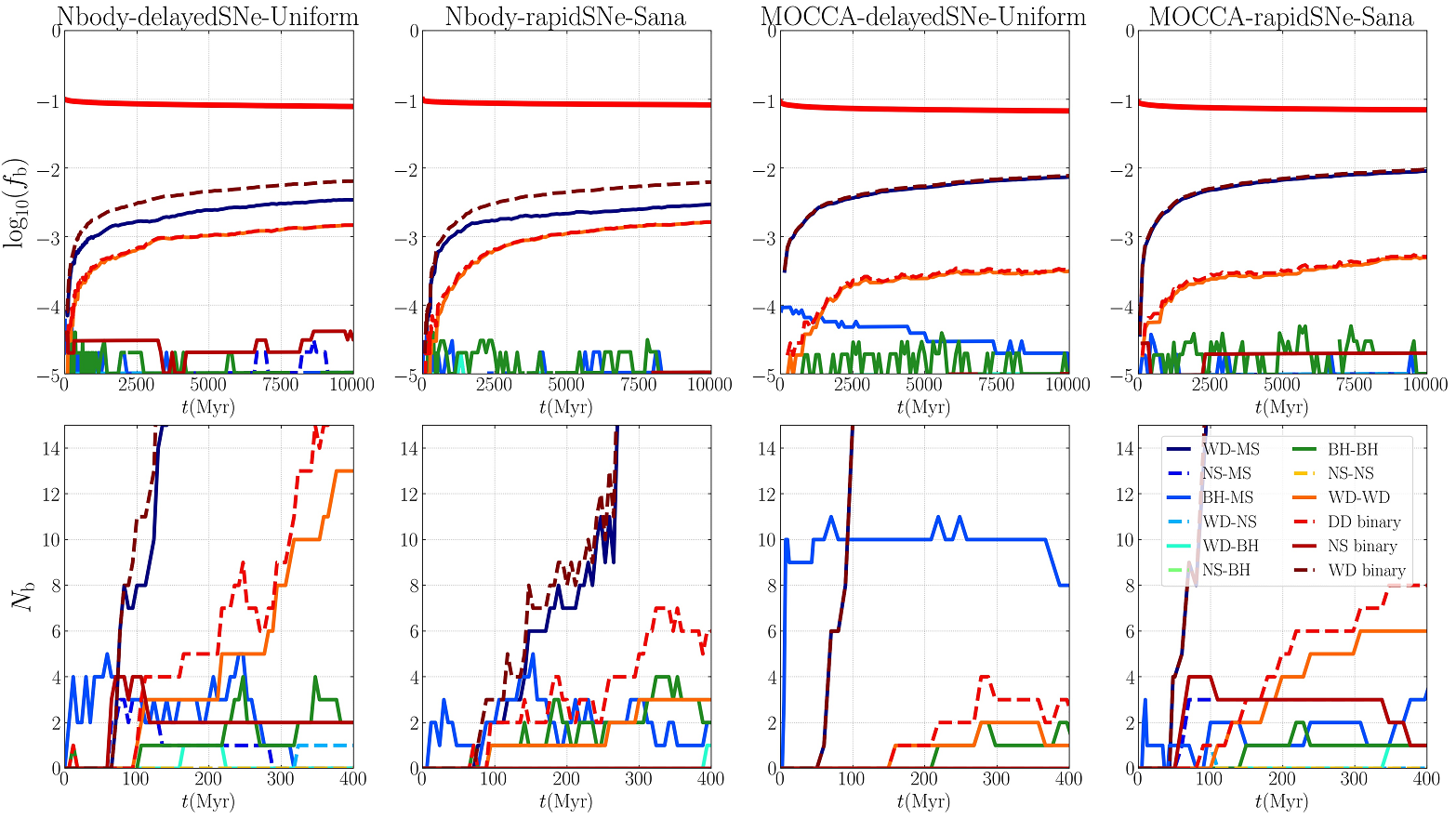
Figure 4: Time evolution over 10 Gyr of the logarithmic (compact) binary fractions (top row) for the Nbody-delayedSNe-Uniform, Nbody-rapidSNe-Sana, MOCCA-delayedSNe-Uniform and MOCCA-rapidSNe-Sana simulations from left to right, respectively. Shown in the top row as a thick red line are the overall logarithmic binary fractions. On the bottom row for the first 400 Myr the absolute number of the double-degenerate (DD), NS, WD, WD-MS, NS-MS, BH-MS, WD-NS, WD-BH, NS-BH, BH-BH, NS-NS and WD-WD binaries are shown.

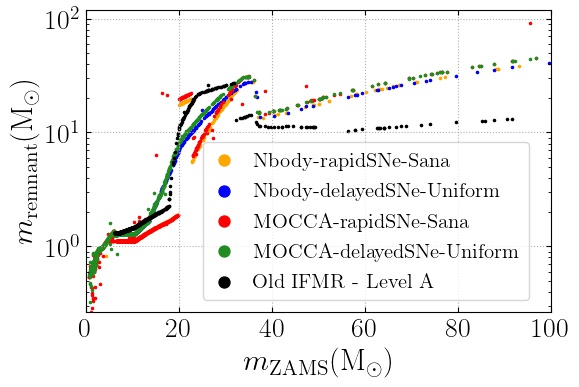
Figure 5: Initial-Final mass relation (IFMR) for the escaping compact objects. The Nbody-delayedSNe-Uniform, Nbody-rapidSNe-Sana, MOCCA-delayedSNe-Uniform and MOCCA-rapidSNe-Sana simulations are shown in red, green, blue and yellow, respectively. The black points show BH masses from another $N$-body simulation with Level A parameters (Belczynski et al., 2002).

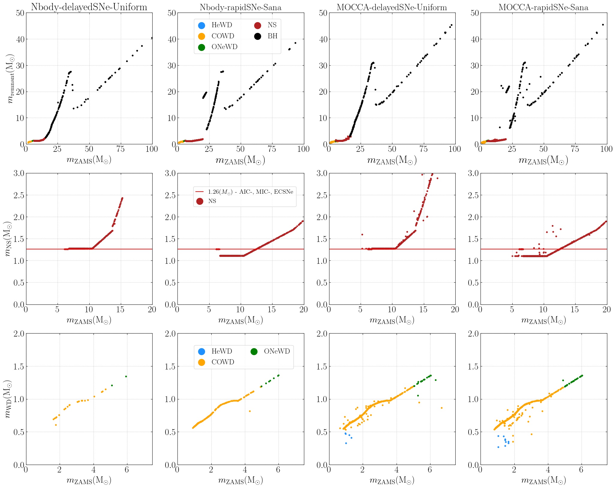
Figure 6: Initial-Final mass relations (IFMR) for the escaping compact objects. From left to right, there are shown the Nbody-delayedSNe-Uniform, Nbody-rapidSNe-Sana, MOCCA-delayedSNe-Uniform and MOCCA-rapidSNe-Sana simulations, respectively. From top to bottom, there are plotted the IFMRs for the BHs, NS and WDs, the IFMRs of the NSs only and the IFMRs for the WDs, respectively. The top IFMRs show excellent agreement with Fryer et al. (2012); Banerjee et al. (2020). The bottom WD IFMR likewise compares well to Han et al. (1995); Hurley et al. (2000); Hurley & Shara (2003). Interestingly, the IFMR shows some NSs escaping at a mass of 1.26 $\text{M}_{\odot}$ (ECSNe, AIC or MIC) for all simulations even with small natal kicks following Gessner & Janka (2018).

4.2.2 Remnant masses

The remnant masses of the compact objects which have escaped the simulation are shown in the Initial-Final mass relation (IFMR) in Fig.5, where the initial mass is the ZAMS mass and the final mass denotes the compact remnant mass. These remnant masses are mainly determined by our choices of either the delayed SNe or the rapid SNe (Fryer et al., 2012) and the lack of an enabled (P)PSINe mechanism. The masses of the compact objects in the MOCCA simulations appear to lie systematically above those of the Nbody6++GPU simulations. There exists one very high mass BH of mass $91.830$ $\rm M_{\odot}$ for the MOCCA-rapidSNe-Sana simulation, which escaped at $1.298$ Gyr. This BH has a complex history and it was subject to an initial binary merger due to stellar evolution. The progenitor stellar mass was $95.618$ $\rm M_{\odot}$. If a (P)PISNe scheme was enabled, then we would never reach these high BH masses of $91.830$ $\mathrm{M}_{\odot}$. The resulting BH would have been capped at $40.5$ $\mathrm{M}_{\odot}$ if we had used psflag=1 & piflag=2 (Belczynski et al., 2016), for example. Also shown in this figure, is an old IFMR from Belczynski et al. (2002). These black dots clearly lie below all the compact objects from the new delayed and rapid SNe prescriptions in the range of (30-100)$\mathrm{M}_{\odot}$. We also see that the difference in the delayed and rapid SNe prescription is mostly in the regime up to around $30.0$ $\mathrm{M}_{\odot}$ at our metallicity of $0.00051$. Therefore, the choice of nsflag/compactmass mostly affects the regime $<30.0$ $\mathrm{M}_{\odot}$. At larger ZAMS masses, all four simulations mostly coincide in their IFMRs. For the rapidSNe simulations, we see the double core-collapse hump, whereas for the delayedSNe simulations, we only see one hump (Fryer et al., 2012).
In Fig.6, we see a more detailed IFMR for each individual simulation, where we also zoom in on the NSs (middle row) and the WDs (bottom row) for all simulations. Apart from the already discussed larger spread in the remnant masses of the compact objects in the MOCCA simulations, the simulations show good consistency with each other, as well as the literature Fryer et al. (2012). This is also true for the WD masses, which are unaffected by the delayed or rapid SNe mechanisms and which follow the original SSE algorithm (Han et al., 1995; Hurley et al., 2000; Hurley & Shara, 2003). To add more depth to the analysis, see Fig.7 and Fig.8 for the masses of all the compact objects (BH, NS, ONeWD, COWD, HeWD) versus their distance to the density centre, $r_{\mathrm{dens}}$, as well as the cumulative histograms of the compact object distances for the MOCCA and the Nbody6++GPU simulations, respectively. There are objects in these plots that extend beyond the tidal radius. This is due to the fact that the escape criterion in Nbody6++GPU removes stars once they are further than two times the tidal radius from the density centre. Overall, there a lot more HeWDs both escaping and remaining inside the clusters of the MOCCA simulations over the full 10 Gyr. We know that HeWDs cannot be formed in the stellar evolution of single stars in a Hubble time. They can be formed only in binaries. In MOCCA models the central density is larger than in the $N$-body models, so it is expected that more frequent dynamical interactions force binaries to form HeWDs because of mass transfer.
The COWD numbers and their distributions are similar for all simulations, but there are many more COWD-COWD binaries in the Nbody6++GPU simulations, mirroring findings in Fig.4. The mass and $r_{\mathrm{dens}}$ distributions of the ONeWDs for the MOCCA and Nbody6++GPU simulations are likewise similar, but there are more outlying ONeWDs for the MOCCA simulations, indicating and underlying the point made early about the MOCCA simulations having more interactions across their full evolution: see Fig.1 and 6. The Nbody6++GPU simulations retain slightly larger numbers of NSs inside the cluster than the MOCCA simulations. Additionally, the Nbody6++GPU simulations only retain NSs of masses 1.26 $\rm M_{\odot}$, which is the mass that is assigned for NSs produced by an ECSNe, AIC or MIC. The MOCCA simulations have a much larger spread in the NS masses again underpinning the point that the MOCCA simulations are denser and lead to more interactions between the stars. The BH masses are distributed very dissimilarly. Firstly, the Nbody-delayedSNe-Uniform simulation retains the least BHs up until 10 Gyr; two single BHs and the BH-BH binary (see Tab.2). This BH-BH binary is also the hardest of all BH-BH binaries remaining at 10 Gyr. The MOCCA-rapidSNe-Sana simulation retains the largest number of BHs up until 10 Gyr (around 20 of which two are in a BH-BH binary). This BH-BH binary is the most massive (combined mass of around 60 $\rm M_{\odot}$) and also the most distant to the density centre of this cluster. The MOCCA-delayedSNe-Uniform and the Nbody-rapidSNe-Sana retain similar numbers of BHs and they are also distributed similarly.

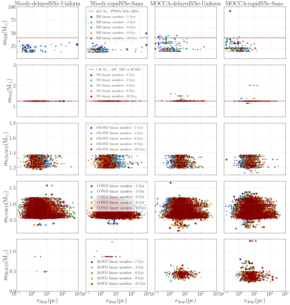
Figure 7: Plot showing the mass of the compact objects in relation to their distance to the density centre $r_{\mathrm{dens}}$(pc) for all four simulations at (1,3,6,9,10) Gyr. From top to bottom the plots show the above information for the BHs, NSs, ONeWDs, COWDs and HeWDs, respectively. BHs: MOCCA retains more BHs than the Nbody6++GPU simulations and all four simulations retain a BH-BH binary at 10 Gyr. NSs: in the Nbody6++GPU runs only the ECSNe, AIC and MIC NSs are retained, whereas there is a larger spread in remnant masses in the MOCCA simulations (which might be due to a post-natal ECSNe, AIC, MIC NS accreting mass). ONeWDs, COWDs: the distributions across all four simulations are very similar. HeWDs: there are many more HeWDs retained in the MOCCA simulations than the Nbody6++GPU simulations at 10 Gyr.

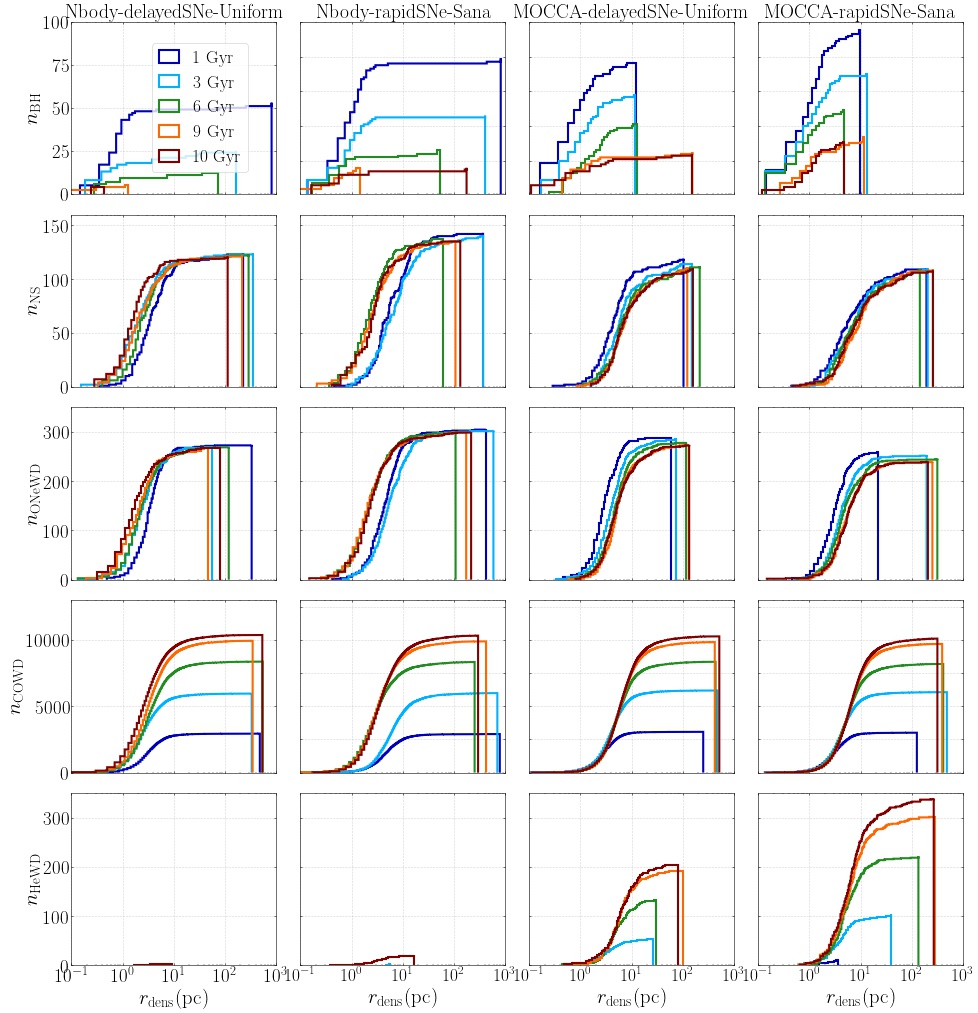
Figure 8: Cumulative distributions for compact object distances to the density centre $r_{\mathrm{dens}}$(pc) for all four simulations at (1,3,6,9,10) Gyr. From top to bottom the plots show the above information for the BHs, NSs, ONeWDs, COWDs and HeWDs, respectively. BHs: Nbody6++GPU simulations retain consistently lower numbers of BHs with the Nbody-delayedSNe-Uniform having the lowest by far (4). NSs: the Nbody6++GPU simulations have consistently slightly larger numbers of NSs retained, but the distributions are very similar. OneWDs and COWDs: distributions and numbers for these objects are very similar. HeWDs: much lower numbers of HeWDs in the Nbody6++GPU simulations than in the MOCCA simulations. If the enabled WD kicks in Nbody6++GPU were the reason, then we would expect to have equally lower numbers of ONeWDs and COWDs as well, but we do not.

4.2.3 Remnant natal kicks and escape speeds

Simulation	type $M_{1}$-$M_{2}$	$M_{1}$($\rm M_{\odot}$)	$M_{2}$($\rm M_{\odot}$)	$e$	$P(\mathrm{days})$	$a(\mathrm{AU})$	$r_{\mathrm{dens}}(\mathrm{pc})$	$t_{\mathrm{GW}}(\mathrm{Gyr})$
Nbody-delayedSNe-Uniform	BH-BH	22.586	17.145	0.415	22452	53.129	0.355	$2.268\times 10^{10}$
Nbody-delayedSNe-Uniform	MS-NS	0.871	1.260	0.479	5271	7.600	1.727	/
Nbody-delayedSNe-Uniform	NS-COWD	1.260	0.892	0.729	56863	37.361	5.535	$2.712\times 10^{12}$
Nbody-rapidSNe-Sana	BH-BH	18.275	20.969	0.953	24207	55.655	0.749	$4.773\times 10^{6}$
Nbody-rapidSNe-Sana	NS-MS	1.260	0.553	0.766	133522	62.343	12.920	/
MOCCA-delayedSNe-Uniform	BH-BH	29.910	19.747	0.940	31703	72.060	0.108	$1.616\times 10^{7}$
MOCCA-delayedSNe-Uniform	NS-MS	1.260	0.767	0.889	3517620	572.904	2.018	/
MOCCA-rapidSNe-Sana	BH-BH	29.905	31.032	0.329	22269	60.963	0.811	$1.598\times 10^{10}$
MOCCA-rapidSNe-Sana	BH-MS	21.156	0.104	0.772	9223	23.845	3.3775	/
MOCCA-rapidSNe-Sana	NS-MS	1.260	0.343	0.801	153356	65.626	7.575	/

Table 2: Table listing the orbital properties of some degenerate binaries surviving inside the cluster at time 10 Gyr with at least one member being a BH or a NS. Also shown is the expected merger timescale $t_{\mathrm{GW}}$ for the compact binaries computed from Peters & Mathews (1963); Peters (1964). None of these compact binaries would be relevant for aLIGO or aVirgo detections.

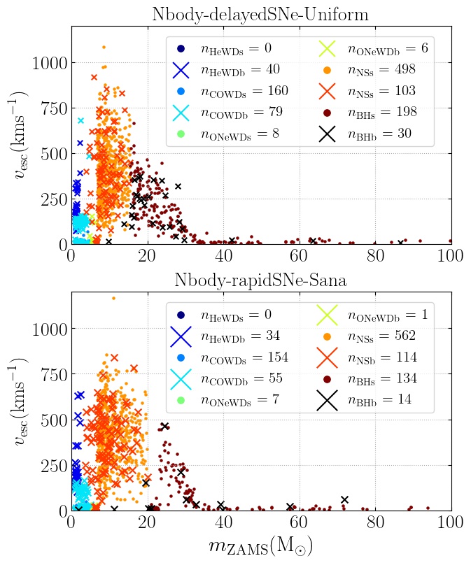
Figure 9: Plot showing the final escape speeds $v_{\mathrm{esc}}(\mathrm{kms}^{-1})$ of the compact objects (WDs, NSs, BHs) for the Nbody-delayedSNe-Uniform and the Nbody-rapidSNe-Sana simulations. Also shown in crosses are the compact objects that come from primordial ZAMS binary stars ($n_{\mathrm{HeWDb}},n_{\mathrm{COWDb}},n_{\mathrm{ONeWDb}},n_{\mathrm{NSb}},n_{\mathrm{BHb}}$), whereas the smaller dots display compact objects originating from ZAMS single stars ($n_{\mathrm{HeWDs}},n_{\mathrm{COWDs}},n_{\mathrm{ONeWDs}},n_{\mathrm{NSs}},n_{\mathrm{BHs}}$). The number counts $n_{\mathrm{HeWDb}},n_{\mathrm{COWDb}},n_{\mathrm{ONeWDb}},n_{\mathrm{NSb}},n_{\mathrm{BHb}},n_{\mathrm{HeWDs}},n_{\mathrm{COWDs}},n_{\mathrm{ONeWDs}},n_{\mathrm{NSs}},n_{\mathrm{BHs}}$ are recorded in the plot legend.

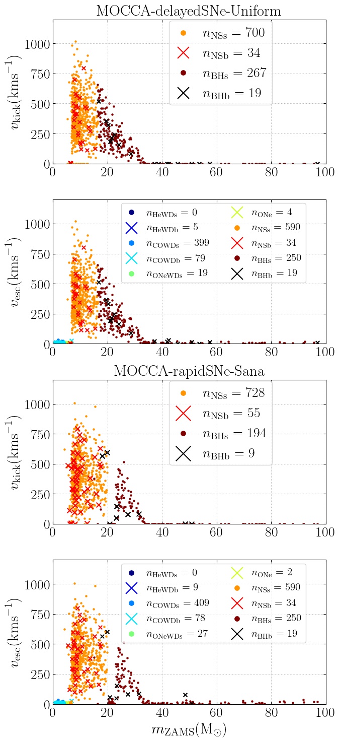
Figure 10: Plot showing the natal kick speeds $v_{\mathrm{kick}}(\mathrm{kms}^{-1})$ of the NSs and BHs (not recorded for WDs), as well as the final escape speeds $v_{\mathrm{esc}}(\mathrm{kms}^{-1})$ of all the compact objects (HeWDs, COWDs, ONeWDs, NSs, BHs) for the MOCCA-delayedSNe-Uniform (top two panels) and the MOCCA-rapidSNe-Sana (bottom two panels) simulations. Also shown in crosses are the compact objects that come from primordial ZAMS binary stars ($n_{\mathrm{HeWDb}},n_{\mathrm{COWDb}},n_{\mathrm{ONeWDb}},n_{\mathrm{NSb}},n_{\mathrm{BHb}}$), whereas the smaller dots display compact objects originating from ZAMS single stars ($n_{\mathrm{HeWDs}},n_{\mathrm{COWDs}},n_{\mathrm{ONeWDs}},n_{\mathrm{NSs}},n_{\mathrm{BHs}}$). The number counts $n_{\mathrm{HeWDb}},n_{\mathrm{COWDb}},n_{\mathrm{ONeWDb}},n_{\mathrm{NSb}},n_{\mathrm{BHb}},n_{\mathrm{HeWDs}},n_{\mathrm{COWDs}},n_{\mathrm{ONeWDs}},n_{\mathrm{NSs}},n_{\mathrm{BHs}}$ are recorded in the plot legend. The compact objects with a zero kick velocity have a constant value of $0.0001$ $\mathrm{kms}^{-1}$ added to them to make them visible.

In Fig.9, the escape speeds $v_{\mathrm{esc}}$ of the compact objects in relation to their ZAMS mass are shown for the Nbody6++GPU simulations. The absolute number of the objects per stellar type are shown and we distinguish between objects coming from either a ZAMS single star or ZAMS binary. This information, as well as the kick speeds $v_{\mathrm{kick}}$ for the NSs and BHs for the MOCCA simulations, is also shown in Fig.10. For the MOCCA simulations, we computed the escape speeds $v_{\mathrm{esc}}$ from their escape energies infinitely far away from the cluster.
First, we discuss the WDs, for which we have the $v_{\mathrm{esc}}$ information readily available across all four simulations. All escaping HeWDs originate from ZAMS binaries in both simulations, which is expected from mass transfer in binaries and the production pathways of HeWDs in general. Their escape speeds reach a couple of hundred $\mathrm{kms}^{-1}$ in some instances for the Nbody6++GPU simulations. This is not the case for the MOCCA simulations. Comparing this with Fig.7 and Fig.8, there are still single HeWDs retained in both the Nbody6++GPU and MOCCA simulations, but a lot fewer for the Nbody6++GPU simulations than for the MOCCA simulations and on the other hand, many more HeWDs escape the Nbody6++GPU simulations than the MOCCA simulations.
Many more COWDs originating from ZAMS singles stars escape than those with a ZAMS binary origin in the Nbody6++GPU runs. The same is true for the MOCCA simulations, but here many more COWDs originating from ZAMS singles escape than from the Nbody6++GPU simulations. In the Nbody6++GPU simulations the escape speeds of the escaping COWDs from ZAMS binaries are much larger than those of the COWDS from ZAMS singles. This should be expected, because if the binary companion underwent a SNe event, the COWD or progrenitor might have adopted the binary’s high orbital speed. In the MOCCA simulation, however, the COWDs (and all other WD types) from ZAMS singles and ZAMS binaries escape with highly uniform $v_{\mathrm{esc}}$. This needs to be investigated further in the future. In total, there are many more COWDs and ONeWDs retained for all simulations than those that escape (see Fig.7 and 8). Consistently more ONeWDs escape the MOCCA simulations from singles and binary ZAMS stars. Future studies into the impact of WD natal kicks on binary stability, escape speeds and escaper number are needed going forward.
The BHs and NSs are affected by the delayed and rapid SNe as well as the fallback-scaled natal kicks, while the WDs are not. We see that compared with the Nbody6++GPU simulations, the distributions of the BH and NS escape speeds are very similar. The KMECH=1 in Nbody6++GPU and the bhflag_kick=nsflag_kick=3 settings in MOCCA for the fallback-scaled momentum conserving kicks, compare also Fig.14 and 15, lead to very similar distributions in escape speeds. It also shows that escape speeds and the natal kick speeds of the MOCCA simulations are very similar. To clarify again, $v_{\mathrm{kick}}$ and $v_{\mathrm{esc}}$ describe the actual natal kick velocity and the velocity at escape from the cluster, respectively. The speeds for the escaping NSs in all four simulations reach up to $10^{3}$ $\mathrm{kms}^{-1}$.
The NSs produced from AIC, ECSNe and MIC lead to very low escape speeds as a result of the very low natal kicks, which we assign by using ECSIG=sigmac=3.0 $\mathrm{kms}^{-1}$ from Gessner & Janka (2018). Even still, some of these NSs escape from all clusters without any significant acceleration. This may be due to evaporation, where a series of weak encounters finally leads to an escape of the NS, or by a strong dynamical ejection. Another reason might be their involvement in a binary, i.e., they were a member of a binary and the binary snaps due to the SN of its companion, causing the star to adopt the high orbital speed of the binary (similar to the proposed mechanism for the high $v_{\mathrm{esc}}$ for some HeWDs and COWDs in the Nbody6++GPU simulations).
The low mass BHs in the delayedSNe simulations also reach $10^{3}$ $\mathrm{kms}^{-1}$, whereas the low mass BHs just at the transition between the NSs and BHs in the rapidSNe simulations are very low, leading to a small gap in velocity distribution of the escaping BHs. This is due to the first of the two core-collapse humps in the remnant mass distribution of the rapid SNe scheme (Fryer et al., 2012; Banerjee et al., 2020); the larger the fallback, the lower the natal kick of the NS or BH. Nevertheless, even some BHs in this gap escape all rapidSNe simulations, which is a result of the low masses of the clusters and thus the low escape speeds. In realistically sized GCs, these BHs would probably not escape, unless through some hard encounter. The larger the ZAMS mass, the lower the resulting escape speed and natal kicks are, due to increasing fallback. This is why at the high end of the BH mass spectrum, the velocities become very small (only a couple of $\mathrm{kms}^{-1}$) in all simulations.

4.2.4 Binary parameters

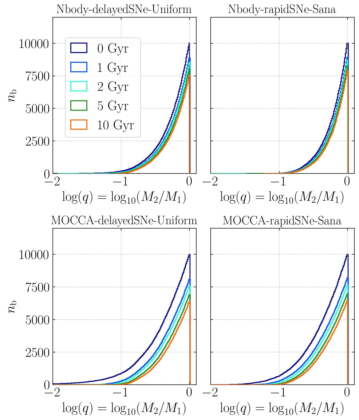
Figure 11: Cumulative histogram showing the mass ratio at times (1,2,5,9,10) Gyr of the binaries for all four simulations. The mass ratio $q$ is calculated such that the lower mass $M_{2}$ is divided by the larger mass $M_{1}$.

The only different initial binary parameters between the delayedSNe-Uniform and the rapidSNe-Sana simulations is the binary mass ratio distribution $q$, which is set to $q_{\text{Uniform}}$ and $q_{\text{Sana}}$, respectively. The binary mass ratios for all four simulations at times (1,2,5,9,10) Gyr are presented in Fig.11. The evolution across all simulations leads to very similar distributions at 10 Gyr with only a few very large binary mass ratios. We note that strictly speaking the $q_{\text{Uniform}}$ and $q_{\text{Sana}}$ initial distributions are very similar overall and thus it is not surprising, but rather reassuring, that this is indeed the case in the simulations. We also see similarities in the semi-major axes $a$ of the binaries as shown in Fig.12. The shape of the curve is roughly what we would expect, since they are distributed flat in log($a$), however, for the Nbody-rapidSNe-Sana there is a small clustering at wide binaries in the cumulative distribution. This can more easily be seen as an unusual increase in the cumulative histogram of the binary eccentricities at low eccentricities in Fig.13. This might be due to a change in regularisation, when the binaries move in and out of KS regularisation. Some testing has been done and we can confirm that this issue is definitely not related to stellar evolution and needs to be resolved in the future. Interestingly, this clustering does not seem to be present in the Nbody-delayedSNe-Uniform simulation. Therefore, it might be related to the hardware or technical parameters within the initialisation of the simulations. However, we did not change any of these between the two Nbody6++GPU simulations and therefore this seems unlikely. We need to explore this erratic issue further and resolve this.

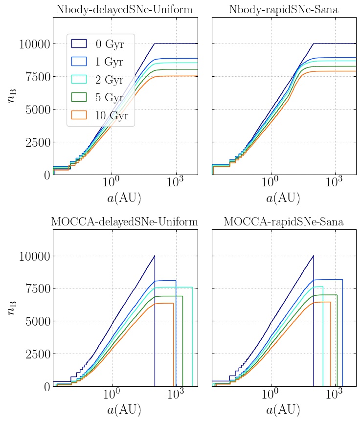
Figure 12: Cumulative histogram showing the semi-major axis $a$(AU) at times (1,2,5,9,10) Gyr of the binaries for all four simulations.

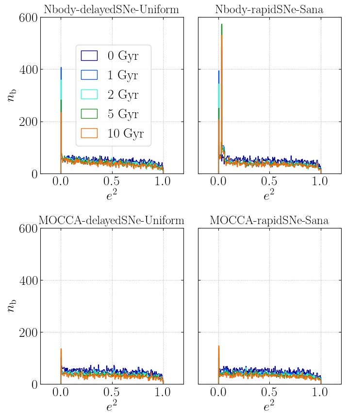
Figure 13: Histogram showing the eccentricity $e^{2}$ at times (1,2,5,9,10) Gyr of the binaries for all four simulations ($N(<e)\propto e^{2}$) for a thermal distribution (Duquennoy & Mayor, 1991)). The Nbody-rapidSNe-Sana simulation reveals a second peak, which might relate to regularisation or another complex origin.

5 Summary, conclusion and perspective

5.1 Summary: direct $N$-body (NBODY6++GPU) and Monte Carlo (MOCCA) simulations

We have compared direct $N$-body (NBODY6++GPU) and Monte Carlo (MOCCA) star cluster models for about 10 Gyr with our updated codes. We showcase the effect of parts of the updated stellar evolution, more specifically the delayed vs. rapid SNe as extremes for the convection-enhanced neutrino-driven SNe paradigm by Fryer et al. (2012) with standard momentum conserving fallback-scaled kicks in combination with metallicity dependent winds from Vink et al. (2001); Vink & de Koter (2002, 2005); Belczynski et al. (2010) and low-kick ECSNe, AIC and MIC (Podsiadlowski et al., 2004; Ivanova et al., 2008; Gessner & Janka, 2018; Leung et al., 2020a). The BHs had no natal spins set (corresponding to the Fuller model in Banerjee (2021b) from Fuller & Ma (2019); Fuller et al. (2019)). The initial model with the delayed SNe enabled had the binary mass ratios uniformly distributed ($q_{\text{Uniform}}$) and is dubbed delayedSNe-Uniform, whereas the initial model with the rapid SNe enabled, had the binary mass ratios distributed as inspired by observations following Kiminki et al. (2012); Sana & Evans (2011); Sana et al. (2013); Kobulnicky et al. (2014) ($q_{\text{Sana}}$) and is dubbed rapidSNe-Sana. The MOCCA models did not employ WD kicks, whereas the Nbody6++GPU models used WD natal kicks following Fellhauer et al. (2003). The time-steps pts1, pts2 & pts3 of MOCCA represent fractions of stellar lifetimes in the main sequence, sub-giant, and more evolved phases that are taken as stellar-evolutionary time steps in the respective evolutionary stages and should, after calibrating them with Startrack (Belczynski et al., 2008), follow the suggestions by Banerjee et al. (2020): pts1=0.001, pts2=0.01 and pts3=0.02. In the Nbody6++GPU simulations, the time-steps pts2 & pts3 are all accounted for by pts2. Here, we chose pts1=0.05 and pts1=0.02. We make the following observations:

• Globally, the star cluster models evolve differently. The mass loss from Nbody6++GPU is slightly lower than that from the MOCCA simulations. The Nbody6++GPU simulations have consistently larger $r_{\mathrm{Lagr}}$ than the MOCCA simulations (see Fig.1). In particular, the half-mass radii are significantly larger than those in the MOCCA simulations. Fig.2 shows us that core collapse happens a bit later in the MOCCA simulations and this is connected with the time-scaling. In the Monte Carlo models the global cluster evolution rate is governed according to Hénon’s principle by the heat flow through the half-mass radius. So for smaller half-mass radius and half-mass relaxation time in MOCCA than in Nbody6++GPU models, the MOCCA models have to evolve faster and provide more energy in the core than for the Nbody6++GPU approach. This leads to more dynamical interactions in the core and a small delay in the core-collapse time. Primordial binaries become active earlier as an energy source than in $N$-body. The MOCCA simulations have smaller half-mass radius and mass and therefore the half-mass relaxation time is also smaller. This means that the MOCCA models are overall dynamically older and have evolved faster. Furthermore, from the core radii evolution of the cluster models, we see that MOCCA simulations have a larger central density, which should lead to a larger number of dynamical interactions in these models compared with the Nbody6++GPU runs. All of this is also connected to the treatment of unbound stars in MOCCA. In MOCCA, when a star acquires a high enough energy in relaxation/interaction to become unbound it is immediately removed from simulations. In Nbody6++GPU this is not the case as stars need time to travel across the star cluster system to be removed to a distance of twice the tidal radius from the density centre. Since $r_{\mathrm{t}}$ is very large in our simulations (see Tab.1), this may take a very long timw (on the scale of Gyrs in some cases). During this time the star can undergo relaxation and become a bound star in the cluster yet again (Baumgardt, 2001). When this process is properly accounted for in MOCCA the evolution of Lagrangian radii in MOCCA and Nbody6++GPU are similar and a new version of the MOCCA code includes an upgrade to properly treat these escaped objects.
  

• From the core radii evolution of the cluster models, we see that MOCCA simulations have a larger central density over the whole simulation. This leads to a larger number of dynamical interactions in the MOCCA runs compared with the Nbody6++GPU runs, as can be inferred from the larger scatter in remnant masses in Fig.6. Although the overall binary fractions are similar, the Nbody6++GPU simulations yield consistently larger fractions over 10 Gyr. Due to the denser MOCCA models, binaries will be disrupted and forced to merge at larger rates. Additionally, more blue straggler stars are show in the HRDs of the MOCCA simulations, as can be seen in Fig.3. This means that there must have been more interactions that lead to mass gain to produce these, i.e. this is a result of the denser MOCCA models. In Fig.5, the masses of the escaping NSs for the MOCCA-delayedSNe-Uniform simulation are larger, simply because we found that the maximum NS mass was set to 3.0 $\rm M_{\odot}$, rather than 2.5 $\rm M_{\odot}$ in the other simulations. This maximum NS mass is taken as the upper limit of neutron star masses and follows from causality (Lattimer & Prakash, 2004). This is not a big a problem, however, since the IFMR for the delayed SNe is continuous in this regime. If we had instead set the maximum NS to 2.5 $\rm M_{\odot}$ then all the NSs in the mass range between 2.5 $\rm M_{\odot}$ and 3.0 $\rm M_{\odot}$ would be BHs with the same masses as the NSs. In the future gravitational million-body simulations, we will use 2.5 $\rm M_{\odot}$ in line with recent observations, such as Linares (2018).
  

• The differences in the time-step parameters (pts1, pts2, pts3) and the wind treatment (mdflag=3$\neq$edd_factor=0, where Nbody6++GPU takes into account the bi-stability jump and the MOCCA simulations do not), in combination, might lead to the slight upward shift in values in the IFMR in Fig.5, which otherwise shows excellent agreement in the BHs, NSs and WDs masses across all simulations for both MOCCA & Nbody6++GPU. Further investigations should be done into systematic shifts of the remnant masses between the MOCCA and Nbody6++GPU code. Both of the IFMRs show excellent agreement with the theory from Fryer et al. (2012) and the Nbody7 results from Banerjee et al. (2020). Comparisons with old (Level A) stellar evolution treatments reveal that these core-collapse neutrino-driven SNe schemes produce much larger BH masses for increasing ZAMS masses than what was previously available (Belczynski et al., 2002) and provide a smooth transition to any of the available (P)PISNe treatments (see also Fig.15) if these are switched on.
  

• The fallback-scaled kick distributions for NSs and BHs likewise show excellent agreement across all masses as shown in Figs.9 and 10. All simulations retain NSs formed from an ECSNe, AIC or MIC of mass $1.26$ $\rm M_{\odot}$ (Belczynski et al., 2008) as we see in Figs.7 and 8. But some of these also escape the cluster despite the low natal kick velocity that we set of ecsig=sigmac=$3.0$ $\mathrm{kms}^{-1}$ (Gessner & Janka, 2018) at similar escape speeds, which might be due to the low cluster densities, evaporation (a series of weak encounters), the kick itself or a combination of the above. Overall, the retention fractions and distributions, see Fig.7, 8, of the compact objects across all simulations are very similar. The HeWDs are the big exception which are mostly retained in the MOCCA simulations, in contrast to Nbody6++GPU where virtually all of them escape with large escape speeds. These escape speeds are, however, much larger than the largest permitted HeWD natal kick of $6.0$ $\mathrm{kms}^{-1}$ (Fellhauer et al., 2003) that is set in the Nbody6++GPU simulations and they are also much larger than the escape speeds for the HeWDs from the MOCCA simulations (see Fig.10). All of the escaped HeWDs originate from ZAMS binaries in both the MOCCA and the Nbody6++GPU simulations. Many more COWDs from single ZAMS stars escape the MOCCA simulations than the Nbody6++GPU simulations and the escape speeds are also much more similar and in many cases much lower than those of the Nbody6++GPU runs. COWDs from ZAMS binaries escape all the simulations in similar numbers. The same statements can be made about the ONeWDs. The reasons why the $v_{\mathrm{esc}}$ distributions are so dissimilar cannot be attributed only to the WD kicks in the Nbody6++GPU simulations, because the natal kicks are of very low velocity dispersion. Further studies with MOCCA and Nbody6++GPU on the effects that WD natal kicks have on binary stability and WD production and retention fraction in OCs, GCs and NSCs should be done going forward to shed more light on this particular aspect using the two modelling methods.

Overall, from the detailed comparison, we find very good agreement between the two modelling methods (Nbody6++GPU and MOCCA) when looking at, for example, the remnant mass distributions. This provides mutual support for both methods in star cluster simulations and the stellar evolution implementations in both codes. However, there are also some significant differences in the global evolution of the star cluster simulations with the two modelling methods. An example of these is the striking differences in blue straggler stars from Fig.3, the reasons for which are given above. The conclusion here relates to our initial models and the treatment of unbound stars in MOCCA vs. Nbody6++GPU simulations. In the future, we strongly suggest to not choose massively tidally underfilling initial cluster models with extremely large tidal radii, especially when using MOCCA simulations, to avoid problems with extremely large escape times for unbound objects. In any case, the results invite additional future comparative studies exploring the vast parameter space of star cluster simulations, also in the initial conditions, with direct $N$-body (Nbody6++GPU) and Monte Carlo (MOCCA) simulations using the updated stellar evolution.

5.2 Perspective on future stellar evolution (SSE & BSE) updates

We have identified the following pain points in our SSE & BSE implementations in Nbody6++GPU & McLuster and to a lesser extent MOCCA, where we still have some work to do. The version of MOCCA presented in this paper has the CV behaviour around the orbital period gap and the GR merger recoil and final post-merger spins, as well as some earlier implementation of modelling high mass and metal-poor Population III stars (Tanikawa et al., 2020) available. An even more up-to-date version by Belloni et al. (2020b) also has an advanced treatment of the wind velocity factor $\beta_{\text{W}}$ as an option. Overall, we will include the stellar evolution routines listed below in the codes MOCCA, Nbody6++GPU & McLuster in the next iteration of stellar evolution updates and refer to these necessary updates below as Level D, see also Appendix A. The (technical) details of these implementations are not shown in Tab.5 and are reserved for a future publication in the interest of brevity.

1. CVs and the orbital period gap The proper behaviour of the CVs around the so-called orbital period gap, which is located at 2 hr $<P_{\mathrm{orb}}<$ 3 hr (Knigge, 2006; Schreiber et al., 2010; Zorotovic et al., 2016), cannot be reproduced by Nbody6++GPU, however, in MOCCA since the BSE modifications by Belloni et al. (2018b) and discussions by Belloni et al. (2017a) are accounted for, this behaviour can be modelled according to our best current understanding. The BSE algorithm of Nbody6++GPU is still in its original form to treat CVs and includes only a simple description of the evolution of accreting WD binary systems given that comprehensive testing of degenerate mass-transfer phases was beyond the original scope of Hurley et al. (2002). The changes that need to be done and we are implementing at the moment in Nbody6++GPU require a lot of modifications. Firstly, the original mass transfer rate onto any degenerate object (KW $\geq 10$) in MOCCA has been upgraded from Whyte & Eggleton (1980); Hurley et al. (2002); Claeys et al. (2014) by including the formalism following Ritter (1988). The angular momentum loss in a close interacting CV that happens as a consequence of mass transfer is called the consequential angular momentum loss mechanism (CAML). Depending on the driving process behind the mass transfer it is either referred to as classical CAML (cCAML) (King & Kolb, 1995) or empirical CAML (eCAML) (Schreiber et al., 2016). The original BSE formalism can also be chosen (Hurley et al., 2002). The eCAML is more empirically motivated by including nova eruptions as the source of additional drag forces. Here the CAML is stronger for low mass WDs. Furthermore, Belloni et al. (2018b) introduced new, completely empirical normalisation factors for magnetic braking (MB) angular momentum loss and gravitational multipole radiation (GMR) angular momentum loss in the case of cCAML following Knigge et al. (2011) and in the case of eCAML, these normalisation factors for MB and GMR follow Zorotovic et al. (2016). The merger between a MS star and its WD companion is now treated with the variable qdynflag, for which if set to 0 the merger assumes no CAML, if set to 1 the merger depends on classical cCAML and if set to 2 the merger depends on empirical CAML (Schreiber et al., 2016). Moreover, Belloni et al. (2018a) improved the stability criteria for thermally unstable mass transfer depending on a critical mass ratio between the primary and secondary star (Schreiber et al., 2016) in the original BSE (Hurley et al., 2002), because the mass transfer rates for thermal timescale mass transfer are underestimated in the original BSE. All of these changes are further complemented by a large reduction in the time-steps for interacting binaries, depending on the factor that may be chosen freely. These upgrades in MOCCA, and soon to be included in Nbody6++GPU, will have the following impact. Firstly, the spins will be properly treated in response to the updated magnetic braking. Secondly, the inflation above and below the orbital period gap and the deflation in the orbital period gap of the donor primary star will be described correctly. Lastly, the processes of GR that lead to angular momentum loss and bloating below the orbital period gap and of MB, which leads to angular momentum and bloating above the orbital period period gap, will be accounted for.
   

2. More on magnetic braking As mentioned above, the MB mechanisms were updated in Belloni et al. (2018b). The original version in Hurley et al. (2002) has been improved by Belloni et al. (2018b) to include the more rigorous treatment by Rappaport et al. (1983), which may be switched on in MOCCA. Then, this new implementation was applied to CVs in GCs in the MOCCA study in Belloni et al. (2019). This model was expanded further in Belloni et al. (2020a) by also adding the so-called reduced magnetic braking model, which extends the previous works to magnetic CVs. An issue that remains in both MOCCA and Nbody6++GPU is the limit for applying MB, which arrives from the fact that MB is only expected to operate in MS stars with convective envelopes. This affects low-mass accreting compact object binaries, such as CVs and low-mass X-ray binaries. In StarTrack (Belczynski et al., 2008), there is such a mass limit imposed. At metallicities of $Z\geq 0.02$, the maximum mass is set to 1.25 $\mathrm{M}_{\odot}$ and for low metallicties at $Z\leq 0.001$, i.e. also at the metallicity used in the simulations of this paper, this limit should be 0.8 $\mathrm{M}_{\odot}$. Additionally, unlike StarTrack, the magnetic braking does not depend on the stellar type KW in MOCCA and in the Nbody6++GPU BSE algorithm, which should be the case, as the MB upper mass limit depends on it.
   

3. Extending SSE fitting formulae to extreme metal-poor (EMP) stars - In $N$-body simulations that use SSE & BSE to model the stellar evolution, any extrapolation beyond $100$ $\mathrm{M}_{\odot}$ should be used with caution (Hurley et al., 2000). However, this mass can be reached in the initial conditions when an IMF above $100$ $\mathrm{M}_{\odot}$ is used, e.g. Wang et al. (2021), or can be reached through stellar collisions Kremer et al. (2020b), especially in the beginning of the simulations (Morawski et al., 2018, 2019; Di Carlo et al., 2019, 2021; Rizzuto et al., 2021b; Rizzuto et al., 2021a). The fact the masses in these simulations sometimes reach masses largely in excess of the original upper mass limit to the fitting process employed in Hurley et al. (2000) cannot simply be ignored. To this end, Tanikawa et al. (2020) devised fitting formulae for evolution tracks of massive stars from $8$ $\mathrm{M}_{\odot}$ up to $160$ $\mathrm{M}_{\odot}$ in extreme metal-poor environments ($10^{-8}\leq Z/Z_{\odot}\leq 10^{-2}$), which can be easily integrated into existing SSE & BSE code variants. These formulae are based on reference stellar models that have been obtained from detailed time evolution of these stars using the HOSHI code (Takahashi et al., 2016, 2019) and the 1-D simulation method described in Yoshida et al. (2019). In a further study with the same method Tanikawa et al. (2021) provide fitting formulae of these stars that go up to even 1260 $\mathrm{M}_{\odot}$ and recently, these are now available up to 1500 $\mathrm{M}_{\odot}$ (Hijikawa et al., 2021). In general, BSE& SSE variants need this implementation, which is already available in MOCCA (although not fully tested), to accurately model the evolution of these extremely-metal poor stars (e.g. Population III) star clusters, high mass stars in some extremely metal poor GCs and to use IMFs, which go beyond $100$ $\mathrm{M}_{\odot}$, e.g. Wang et al. (2021), for these clusters. Adding the Tanikawa et al. (2020) capability is especially interesting as for the first time we might be able to model extremely massive stars (many hundreds and even thousands of $\mathrm{M}_{\odot}$) in massive GC environments. We note that there are likely some intrinsic differences between the standard SSE (Hurley et al., 2000) and the new fitting formulae by Tanikawa et al. (2020), because the former were fitted to the STARS stellar evolution program (Eggleton, 1971, 1972, 1973; Eggleton et al., 1973; Pols et al., 1995) results and latter to the afore-mentioned HOSHI code (Takahashi et al., 2016, 2019). This becomes particularly relevant when attempting to mix low mass stars ($\mathrm{M}_{\odot}\leq 8$) modelled with the traditional fitting formulae in the SSE code and high mass stars modelled by Tanikawa et al. (2020). Moreover, the formulae by Tanikawa et al. (2020) are only valid for masses larger than 8 $\mathrm{M}_{\odot}$ and thus we need a sensible transition between Hurley et al. (2000) and Tanikawa et al. (2020).
   
   

4. Masses of merger products In the most recent version of StarTrack, the merger products of certain stellar types were assigned new merger masses (Olejak et al., 2020). The problem in the old BSE (Hurley et al., 2002) arises from the fact that the mass of the product of a merger during dynamically unstable mass transfer, especially MS-MS merger, leads to $M\simeq M_{\mathrm{accretor}}$. There are many contact or over-contact MS-MS binaries that appear to be stable. On the other hand, there are also blue straggler stars and very massive stars ($>150$ $\mathrm{M}_{\odot}$) that are believed to be merger products, e.g. stars R136a, R136b and 136c in the large Magellanic cloud (Bestenlehner et al., 2020) and the two stars WR 102ka in the Milky Way (Hillier et al., 2001; Barniske et al., 2008) are estimated to have masses exceeding 200 $\mathrm{M}_{\odot}$. To account for this, Olejak et al. (2020) have introduced formalisms along the lines of $M=M_{\mathrm{accretor}}+f_{\mathrm{x}}\times M_{\mathrm{donor}}$, for a number of different merger scenarios involving different stellar types. Here $f_{\mathrm{x}}$ should be in the range of 0.5-1.0. This is still a very simple picture of stellar mergers and we need to elaborate on this approach. With the old BSE formalism, we may significantly reduce the cluster mass, which therefore also affects its evolution. This might be specially true when using the Sana orbital period distribution from McLuster initial conditions (adis=6) (Kiminki et al., 2012; Sana & Evans, 2011; Sana et al., 2013; Kobulnicky et al., 2014), which has a lot of massive primordial MS-MS binaries with periods $P_{\mathrm{orb}}$ shorter than a few days.
   

5. GR merger recoil and final post-merger spins The latest studies of IMBH growth with Nbody6++GPU (Di Carlo et al., 2019; Di Carlo et al., 2020a; Di Carlo et al., 2020b, 2021; Rizzuto et al., 2021b; Rizzuto et al., 2021a) do not include a general relativistic merger recoil treatment (in addition to missing PN terms). But Arca-Sedda et al. (2021) have included the recoil kicks by a posteriori analysis. The GR merger recoil is also missing from the MOCCA Survey Database I (Askar et al., 2017). Nbody7 and also the current development version of Nbody6++GPU contain a proper treatment of such velocity kicks. They depend on spins and mass ratio, and are caused due to asymmetric GW radiation during the final inspiral and merger process. Numerical relativity (NR) models (Campanelli et al., 2007; Rezzolla et al., 2008; Hughes, 2009; van Meter et al., 2010) have been used to formulate semi-analytic descriptions for MOCCA and Nbody codes (Morawski et al., 2018, 2019; Banerjee, 2021b; Belczynski & Banerjee, 2020; Arca-Sedda et al., 2021; Banerjee, 2021a). For (nearly) non-spinning BHs (Fuller model), the kick velocity is smaller than for high spins. In the case of large mass ratios the kick velocity is much smaller than for small mass ratios (Morawski et al., 2018, 2019) and therefore, in extreme cases these post-merger BHs might even be retained in open clusters (Baker et al., 2007, 2008; Portegies Zwart et al., 2010; Schödel et al., 2014; Baumgardt & Hilker, 2018). For non-aligned natal spins and small mass ratios on the other hand, the asymmetry in the GW may produce GR merger recoils that reach thousands of $\mathrm{kms}^{-1}$ (Baker et al., 2008; van Meter et al., 2010).
   Generally, the orbital angular momentum of the BH-BH dominates the angular momentum budget that contributes to the final spin vector of the post-merger BH and therefore, within limits, the final spin vector is mostly aligned with the orbital momentum vector (Banerjee, 2021b). In the case of physical collisions and mergers during binary-single interactions, the orbital angular momentum is not dominating the momentum budget and thus the BH spin can still be low. Banerjee (2021b) also includes a treatment for random isotropic spin alignment of dynamically formed BHs. Additionally, Banerjee (2021b) assumes that the GR merger recoil kick velocity of NS-NS and BH-NS mergers (Arca Sedda, 2020; Chattopadhyay et al., 2021) to be zero but assigns merger recoil kick to BH-BH merger products from numerical-relativity fitting formulae of van Meter et al. (2010) (which is updated in Banerjee 2021a). The final spin of the merger product is then evaluated in the same way as a BH-BH merger.
   With the updates above, in addition to the BH natal spins discussed above, Nbody6++GPU will be able to fully model IMBH growth during the simulation (unlike in post-processing with MOCCA as in Morawski et al. (2018, 2019)) in dense stellar clusters according to our best understanding. This is one of last remaining and important puzzle pieces in our SSE & BSE implementations that helps us to simulate IMBH formation and retention in star clusters and the corresponding aLIGO/aVirgo GW signal (Abbott et al., 2020a).
   

6. Wind velocity factor - the accretion of stellar winds in binaries depends on the wind velocity and a factor $\beta_{\text{W}}$. In the updated binary population synthesis (BPS) code COSMIC by Breivik et al. (2020), the value $\beta_{\text{W}}$ is allowed a broader range of values that actually do depend on stellar type following the StarTrack code by Belczynski et al. (2008). In the MOCCA & Nbody6++GPU versions presented in this paper $\beta_{\text{W}}$=0.125, where this represents the lower limit and should roughly correspond to the wind from the largest stars of $900$ $\text{R}_{\odot}$ (Hurley et al., 2002). In the future, $\beta_{\text{W}}$ will depend on the stellar type.
   

7. Pulsars and magnetic spin field from NSs The COSMIC BPS code (Breivik et al., 2020) includes new BSE additions that properly treat pulsars (Kiel et al., 2008; Ye et al., 2019; Breivik et al., 2020) in an attempt to mirror observations of spin periods and magnetic fields of young pulsars (Manchester et al., 2005). Similarly, the COMPAS BPS code (Stevenson et al., 2017a, b) employs updated BSE and is used to study NS binaries, such as the elusive BH-NS (Chattopadhyay et al., 2021) and NS-NS binaries (Chattopadhyay et al., 2020) using updated pulsar prescriptions. These updates are also present in the earlier BPS code BINPOP by Kiel et al. (2010), which is also based on the original BSE (Hurley et al., 2002). In detached binaries, a magnetic dipole radiation is assumed for the spin-period evolution whereas in non-detached binaries, a so-called magnetic field burying as a response to mass transfer is implemented (Kiel et al., 2008), where the magnetic field decays exponentially depending on the accretion time and the mass that is transferred (equation (7) in Breivik et al. (2020)). Mergers that include a NS produce a NS with a spin period and magnetic field that is drawn again from the same initial distribution, except for millisecond pulsars (MSPs) which stay MSPs after mergers. The magnetic field of a NS cannot be smaller than $5\times 10^{7}$ G (Kiel et al., 2008). In Nbody6++GPU & MOCCA, we need these updates to properly account for the spin and the magnetic field evolution of all pulsars.
   

8. Ultra-stripping in binary stars After CE formation in a hard binary consisting of a NS or a BH and a giant star, the hydrogen-rich envelope of the giant star gets ejected, carrying large amounts of angular momentum with it (Tauris et al., 2013, 2015). After the CE is ejected fully, the NS orbits a naked He star, after which further mass transfer via RLOF may happen (Tauris et al., 2017) depending on the RLOF criteria mentioned above. This leads to stripping of the envelope of the He star until it reaches a naked core of mass $1.5$ $\rm M_{\odot}$ and explodes in a so-called ultra-stripped SNe (USSNe) (Tauris et al., 2013, 2015). According to Tauris et al. (2017) most of these binaries survive the USSNe. Breivik et al. (2020) have an implementation in COSMIC, which allows for this SNe pathway. In their models, the USSNe leads to an ejected mass of $0.1$ $\rm M_{\odot}$. The resulting kick velocity dispersion is much lower than the kick velocity dispersion following Hobbs et al. (2005). In general, there should be a bi-modal kick distribution, where NSs with a mass above $1.33$ $\rm M_{\odot}$ receive large kicks and NSs with masses below that receive small kicks with a kick velocity dispersion of about 20.0 $\mathrm{kms}^{-1}$ (Tauris et al., 2017). Since the USSNe appears to be central to BH-BH, BH-NS and NS-NS merger rates (Schneider et al., 2021), we will work on implementations in Nbody6++GPU & MOCCA. Very recently, Schneider et al. (2021) found that through extreme stellar stripping in binary stars (Tauris et al., 2013, 2015, 2017) in their MESA models (Paxton et al., 2011, 2015), there is an overestimation by 90% in the BH-BH mergers and 25-50% in the BH-NS numbers if only any of the Fryer et al. (2012) prescriptions, rapid or delayed, are enabled. Overall, they predict a slight increase of 15-20% more NS-NS mergers. This will definitely have to be explored in the future in N-body simulations.

We are in the process of implementing the above into the McLuster version presented in this paper and results are reserved for a future publication.
With the updates in the SSE & BSE algorithms of MOCCA & Nbody6++GPU presented in this paper, we are now able to fully model realistic GCs accurately across cosmic time with direct $N$-body simulation and also Monte-Carlo models according to our current understanding of stellar evolution of binary and single stars. Thus, the next step is to test these updates with new direct million-body Dragon-type GC simulations, following on from Wang et al. (2016), and Dragon-like NSC simulations similar to Panamarev et al. (2019), and compare these with MOCCA modelling. In addition to Nbody6++GPU, we will in the future also use the PeTar code by (Wang et al., 2020a, b; Wang et al., 2020c). This code also uses up-to-date SSE & BSE implementations in code structure similar to the original SSE & BSE (Hurley et al., 2000, 2002) and similar to MOCCA. These two direct $N$-body codes in combination with Monte-Carlo models from MOCCA all employing modern stellar evolution will yield unprecedented and exciting results into the dynamical and stellar evolution of star clusters of realistic size.
Finally, we note that a successor to SSE called the Method of Interpolation for Single Star Evolution METISSE (Agrawal et al., 2020) has recently been produced. This utilises advancements in astrophysical stellar evolution codes to provide rapid stellar evolution parameters by interpolation within modern grids of stellar models. Thus it offers the potential for an astrophysically more robust (and potentially faster) realistic alternative to the updated SSE implementation in Nbody6++GPU and MOCCA. However, a similar approach as presented by Agrawal et al. (2020) is not yet available for the BSE routines and thus we will have to wait for a binary stellar evolution version of METISSE. Similarly, the SEVN code (Spera & Mapelli, 2017; Spera et al., 2019; Mapelli et al., 2020b) and its binary version is still a work in progress and at this moment in time not ready to be fully implemented into our codes. Therefore, it is likely that the SSE & BSE presented here and the large number of variants of these codes are destined to stay relevant in the modelling of stellar evolution of single and binary stars for quite some time.

Data Availability

The data from the runs of these simulations will be made available upon reasonable request by the authors. The Nbody6++GPU and McLuster versions that are described in this paper will be made publicly available. The MOCCA version will be available upon reasonable request to MG.

Appendix A Stellar and binary evolution levels A, B, C

The stellar evolution levels and the corresponding options are shown in Tables 3, 4 and 5. The foundation for evolving a single star in the Nbody6++GPU and MOCCA codes and all subsequent updates is provided by the state-of-art population synthesis code SSE (Hurley et al., 2000, 2013b). In this code every evolutionary phase of the star receives an integer related to a certain stellar type KW. These stellar types are divided as such:

• KW$=0\equiv\text{MS star}\quad M\leq 0.7\mathrm{M}_{\odot}$

• KW$=1\equiv\text{MS star}\quad M>0.7\mathrm{M}_{\odot}$

• KW$=2\equiv\text{Hertzsprung Gap (HG)}$

• KW$=3\equiv\text{First Giant Branch (GB)}$

• KW$=4\equiv\text{Core Helium Burning (CHeB)}$

• KW$=5\equiv\text{Early Asymptotic Giant Branch (EAGB)}$

• KW$=6\equiv\text{Thermally Pulsating Asymptotic Giant Branch (TPAGB)}$

• KW$=7\equiv\text{Naked Helium Star MS (HeMS)}$

• KW$=8\equiv\text{Naked Helium Star Hertzsprung Gap (HeHG)}$

• KW$=9\equiv\text{Naked Helium Star Giant Branch (HeGB)}$

• KW$=10\equiv\text{Helium White Dwarf (HeWD)}$

• KW$=11\equiv\text{Carbon-Oxygen White Dwarf (COWD)}$

• KW$=12\equiv\text{Oxygen-Neon White Dwarf (ONeWD)}$

• KW$=13\equiv\text{Neutron Star (NS)}$

• KW$=14\equiv\text{Black Hole (BH)}$

• KW$=15\equiv\text{massless remnant}$

We note, that Nbody6++GPU and MOCCA has another stellar type (for single stars), which is KW=$-1$, which assigns pre-MS stars (Railton et al., 2014). This treatment is valid for stars in the range $0.1-8.0\,\text{M}_{\odot}$ at solar metallicity $Z_{\odot}$=0.02.
The basis for this code are analytic fitting formulae, which are continuous over the entire stellar mass range and approximate the evolution of the stars in the $N$-body simulations depending on their mass $M$ ($\text{M}_{\odot}$), metallicity $Z$ and age $t$ (Myr). The delivered output is stellar luminosity $L$ ($\text{L}_{\odot}$), stellar radius $R$ ($\text{R}_{\odot}$), stellar core radius $R_{\mathrm{c}}$ ($\text{R}_{\odot}$) and core mass $M_{\mathrm{c}}$ ($\text{M}_{\odot}$) and other parameters as a function of those parameters. The SSE code was fitted to detailed stellar models of up to $50\,\text{M}_{\odot}$ and originally tested to be valid for masses from $0.01$ $\text{M}_{\odot}$ up to $100$ $\text{M}_{\odot}$ (where anything above $50$ $\text{M}_{\odot}$ is an extrapolation and usage above $100$ $\text{M}_{\odot}$ was not recommended) and in metallicity ranges from $Z$=$0.0001$ up to $Z$=$0.03$ (Hurley et al., 2000), where the solar metallicity is given by $Z_{\odot}$=$0.02$. They found that the fitted models were accurate to within 5% of the detailed evolutionary tracks.
Stars rarely exist in isolation. In fact, it is expected that most stars are born as twins, so-called primordial binaries (Kroupa, 1995a; Sadavoy & Stahler, 2017; Belloni et al., 2017c). Most of these primordial binaries are disrupted in a star cluster, leaving a star cluster with hard binaries (Milone et al., 2012), which has also been studied with, for example, MOCCA (Leigh et al., 2015). The vicinity to another star or compact object radically changes the evolution of the star as many more processes, which may lead to mass gain or mass loss of the star come into play. The BSE code (Hurley et al., 2002, 2013a) provides the foundation of binary stellar evolution on which all other recent updates stand.
This appendix is devoted to summarise the extensive changes which have been made in the stellar evolution in MOCCA & Nbody6++GPU since Hurley et al. (2000, 2002). We categorise the existing stellar evolution routines in levels. This is because with the increasing number of recipes and complexity therein available, we found it difficult to document and communicate these quickly in our simulations. The stellar evolution options that are available in Nbody6++GPU and MOCCA as of the writing of this paper, are shown in Tables 3, 4 and 5, respectively. We divide the available stellar evolution recipes in Nbody6++GPU & MOCCA as such:

1. Level A - Stellar evolution settings that mirror in part the settings in the Dragon simulations of GCs (Wang et al., 2016) and NSCs (Panamarev et al., 2019) and also the MOCCA Survey DataBase I (Askar et al., 2017). Most of these are outdated and should be generally not be used anymore, see e.g Shu et al. (2021).
   

2. Level B - Stellar evolution settings that have been tested extensively and may be used without concern. A selection of these should be enabled in the next gravitational million-body simulations.
   

3. Level C - Stellar evolution settings that are available in the codes, but those that are not present in level B have not yet undergone sufficient testing and are therefore deemed experimental as of the writing of this paper.
   

4. Level D - Stellar evolution settings that will be added in the next iteration of stellar evolution updates, see also section 5.2 for details on these.

In the more distant future, we will sequentially add new levels (the next one would be level E), where we group further planned stellar evolution updates on top of the preceding level (in this case level D) in Nbody6++GPU, MOCCA & McLuster together. We hope that this will greatly help in the documentation and aid the future user of the codes to properly choose SSE & BSE settings in his or her simulations.

A.1 Dynamical mass transfer and other processes in binary stars

In Nbody6++GPU, the dynamical mass transfer and the stability thereof in Roche-lobe overflow (RLOF) between binary stars is computed by roche.f, which calls subroutines for magnetic braking magbrk.f, for gravitational radiation grrad.f and for coalescing of RLOF or common-evelope evolution (CEE) binaries coal.f. The tidal circularisation and tidal spin synchronisation and associated timescales are set in bsetid.f, which still follow the original treatment by Hurley et al. (2002) and sources therein. In MOCCA, all of the above is included in the original evolv2b.f (Hurley et al., 2002) with lots of more recent updates regarding the proper evolution of cataclysmic variables (CVs) (Belloni et al., 2018b). These updates may be switched off, however, with the parameters camlflagMZ=qdynflagMZ=qtherflagMZ=0 (Belloni et al., 2018b). Therefore, we may still enable the same dynamical mass transfer and stability criteria in Nbody6++GPU and MOCCA based on (Hurley et al., 2002). Here, the stability of the mass transfer is determined by the original relations of radius-mass exponents $\zeta$ by (Webbink, 1985), which give critical mass ratios of the donor and accretor star implemented in Hurley et al. (2002). In semi-detached binaries, the primary loses some mass via winds and the secondary can accrete the material if passing through it. This Bondi-Hoyle accretion rate Bondi & Hoyle (1944) (acc2 in both codes) is sensitive to the wind velocity factor $\beta_{W}$ (Hurley et al., 2002). $\beta_{\text{W}}$ strongly depends on spectral type KW; the larger the star, the lower $\beta_{\text{W}}$ . In the BSE implementation of Nbody6++GPU (and PeTar & Nbody7) this is not the case, unlike in the latest versions of MOCCA (Belloni et al., 2020b), StarTrack (Belczynski et al., 2008) and COSMIC (Breivik et al., 2020). The latter is also implemented in the latest version of CMC (Kremer et al., 2020b). We set beta=0.125 in the simulations following Hurley et al. (2002), where this represents the lower limit and should roughly correspond to the wind from the largest stars of $900\,\text{R}_{\odot}$. The angular momentum factor for mass loss during RLOF in both codes is set by gamm1 in Nbody6++GPU and gamma in MOCCA (Hurley et al., 2002). If positive gamm1=gamma$>0$, then the lost material carries with it a fraction gamma of orbital angular momentum. If set to gamm1=gamma=-1, then the material carries with it specific angular momentum of the primary and if set to gamm1=gamma=-2, then the material is lost from system as if it was a wind from the secondary. The factor to reduce the spin angular momentum change owing to wind accretion is xi and the fraction of accreted matter retained in nova eruption is epsnov in both codes (Hurley et al., 2002).
Accretion rates onto a NS or BH (Eddington and Super-Eddington) are controlled by the parameter eddfac in both codes. Super-Eddington accretion rates are set by (eddfac=100.0) (Cameron & Mock, 1967). The Chandrasekhar mass of a WD is set to MCH = 1.44 $\text{M}_{\odot}$ (Mazzali et al., 2007; Boshkayev et al., 2013). The maximum NS mass is set to mxns$\leq 2.5\,\text{M}_{\odot}$ (Lattimer & Prakash, 2004; Linares, 2018; Baym et al., 2018, 2019). In the mix.f and coal.f subroutines of Nbody6++GPU, (Rizzuto et al., 2021b) implemented a variable FctorCl, that controls the mass accretion if a big star (KW$\,\leq\,$9) merges with a BH or NS. If FctorCl=1, then the whole star is accreted onto the BH or NS. Likewise, if FctorCl=0, then no mass is accreted. MOCCA has a similar variable available called tzo. We include a post-Newtonian (PN) orbit averaged dynamics treatment according to Peters & Mathews (1963); Peters (1964) for binaries containing a NS or BH in grrad.f in Nbody6++GPU and evolv2b.f in MOCCA.
The routine comenv.f and the respective parameters (second row in Tab. 4 and Tab. 5 for Nbody6++GPU and MOCCA, respectively) deal with the common envelope evolution following Hurley et al. (2002), which in turn follows Dewi & Tauris (2000); Tauris et al. (2000). CEE is one of the possible outcomes of RLOF between close binary stars (Paczynski, 1976; Ivanova et al., 2013; Ivanova, 2016; Ivanova et al., 2020). At the end of CEE the envelope of the primary (in some cases also of the secondary) is stripped away and CEE terminates. It is described by two parameters $\alpha_{\mathrm{CE}}$ and $\lambda_{\mathrm{CE}}$; the first one parameterizes what fraction of the orbital energy is used to liberate the envelope; the second one is a factor scaling the binding energy of the envelope. Both codes also allow the addition of some fraction of recombination energy to the binding energy in order to lower the threshold for loss of the envelope, depending on the stellar type. The procedure used is similar, but not identical to Claeys et al. (2014).
Still today, both $\lambda_{\rm CE}$ and $\alpha_{\rm CE}$ remain highly uncertain (Morawski et al., 2018, 2019; Giacobbo & Mapelli, 2018, 2019; De et al., 2020; Santoliquido et al., 2020; Everson et al., 2020; Langer et al., 2020). However, for low-mass stars, given their relatively large numbers in observed samples, such as the post-CE binaries identified by the Sloan Digital Sky Survey (Rebassa-Mansergas et al., 2012), reconstruction techniques and binary population synthesis have allowed us to infer, to some extent, a low value for $\alpha_{CE}$, which is $\sim 0.2-0.3$ (Zorotovic et al., 2010; Toonen & Nelemans, 2013; Camacho et al., 2014; Cojocaru et al., 2017).

A.2 Stellar winds

The routine mlwind.f and the respective parameters (second row in Tab. 4 and Tab. 5 for Nbody6++GPU and MOCCA, respectively) deal with the mass loss from stars via winds and outflows. In Nbody6++GPU and MOCCA the choices of wind prescriptions are determined by mdflag and edd_factor, respectively. Stellar winds and their correct descriptions for our purposes are very important, because they are critical in determining the mass of the compact object progenitors and thus they have a large influence on the compact object mass distributions in the cluster themselves (Belczynski et al., 2010; Giacobbo et al., 2018; Kremer et al., 2020b). In Nbody6++GPU and MOCCA, the options of winds are very different in many places and therefore, these are listed independently below.
First of all, for Nbody6++GPU and mdflag$\leq$2 we apply the mass loss of Nieuwenhuijzen & de Jager (1990) for massive stars over the entire HRD with a metallicity factor from Kudritzki et al. (1989). In the case of giant stars, Nbody6++GPU calculates the mass loss from Kudritzki & Reimers (1978) (with neta=0.477 suggested from McDonald & Zijlstra (2015)). Similarly, for the AGB stars and mdflag$\,\leq\,$2 BSE follows Vassiliadis & Wood (1993) and we apply the reduced Wolf-Rayet (WR)-like mass loss for small H-envelope masses from Reimers (1975); Hamann & Koesterke (1998); Hurley et al. (2000). If mdflag$=$2, then the treatment of luminous blue variable (LBV) winds are added, which follow Humphreys & Davidson (1979, 1994). For mdflag$>$2, these winds follow the LBV winds of Belczynski et al. (2020). If mdflag=3, then for massive and hot O and B-type stars, the code switches on the metallicity dependent winds by Vink et al. (2001); Vink & de Koter (2002, 2005); Belczynski et al. (2010), who established their mass-loss rates for O and B-type from a grid of wind models across a wide range of metallicities ($10^{-5}<Z/Z_{\odot}<10$). Caution is advised against the so-called bi-stability jump, which is the drastic change of the character of the driving (ionisation) line, because of a sudden change in the wind ionisation. There is the option available to have these winds without the bi-stability jump Belczynski et al. (2010) (temperature shifted to the edge of the jump) in Nbody6++GPU (mdflag=4). For more evolved stars starting from naked He stars with KW$\geq$7, with mdflag$\geq$3 the metallicity dependent WR wind factor from Vink & de Koter (2005) is used. For H-rich low mass stars, the mass loss rates remain unchanged Hurley et al. (2000).
In the MOCCA version of BSE, with edd_factor=0, we use fixed $\alpha$ from Giacobbo et al. (2018) in the prescriptions by Belczynski et al. (2010). If edd_factor=1, then the electron-scattered Eddington factor is taken from Gräfener & Hamann (2008) and the exponent of the dependence on metallicity is then calculated from Chen et al. (2015) instead. The rest of the mlwind.f routine uses the same prescriptions for the stars for both edd_factor=0 and edd_factor=1. The LBV-like mass loss beyond the Humphreys-Davidson limit follows Humphreys & Davidson (1994); Belczynski et al. (2010). We apply the mass loss of Nieuwenhuijzen & de Jager (1990) for massive stars over the entire HRD with a metallicity factor from Kudritzki & Reimers (1978). In the case of giant stars, MOCCA calculates the mass loss from Kudritzki & Reimers (1978). If neta$>$0 (neta=0.477 from McDonald & Zijlstra (2015) is suggested), then this mass loss is based on Reimers (1975) and if neta$<$0 it follows a more realistic setting by Schröder & Cuntz (2005), which takes into account the effective temperature and surface gravity of the star (here neta=0.172 is suggested). The winds of the AGB stars follow Vassiliadis & Wood (1993) and we apply the reduced Wolf-Rayet (WR) like mass loss for small H-envelope masses from Reimers (1975); Hamann & Koesterke (1998); Hurley et al. (2000). For massive and hot O and B-type stars, the code switches on the metallicity dependent winds by Vink et al. (2001); Vink & de Koter (2002, 2005); Belczynski et al. (2010). For more evolved stars starting from naked He stars with KW$\geq$7, the MOCCA BSE uses the metallicity dependent WR wind factor from Vink & de Koter (2005). We note that the MOCCA BSE does not account for the aforementioned bi-stability jump, so overall the treatment of the winds from MOCCA and Nbody6++GPU are most similar for mdflag=4 $\simeq$ edd_factor=0.
We note, that today the wind mass loss from very large mass stars in the regime of WR stars still remains very uncertain and is difficult to model (Sander & Vink, 2020; Sander et al., 2020; Higgins & Vink, 2019; Higgins et al., 2021; Vink, 2021). The same can also be said in general about stars on the lower mass end (Decin, 2020). It is likely that we will need to revise our stellar wind mass loss and terminal velocity models many times in the future with this in mind, especially, when we aim to properly model aLIGO/aVirgo GW source progenitor stars.

A.3 Remnant masses of compact objects

The routine hrdiag.f and the respective parameters (first row in Tab. 4 and Tab. 5 for Nbody6++GPU and MOCCA, respectively) deal with the post-SNe remnant masses of the NSs and BHs. In Nbody6++GPU and MOCCA the choices of the NS and BH remnant masses are determined by nsflag and compactmass, respectively. The updated stellar evolution now incorporates a selection of possible SNe pathways, which lead to a variety of remnant masses. In the present versions of the hrdiag.f routine, any of the five remnant-mass schemes following Eldridge & Tout (2004); Belczynski et al. (2002, 2008); Fryer et al. (2012) may be chosen. In this paper the rapid (nsflag=compactmass=3) and delayed (nsflag=compactmass=4) SNe mechanisms are used as extremes for the convection-enhanced neutrino-driven SNe paradigm (Fryer et al., 2012).
In hrdiag.f, we can also set the pulsating pair instability SNe (PPISNe) resulting from electron-positron pair production and subsequent decreasing pressure support in massive He cores. These electron-positron pairs effectively remove pressure from outward photons, until the oxygen in the stellar core ignites in a flash, which creates a pulse and a thermonuclear reaction in the outward direction, after which the core stabilises. In even more massive He cores, the core does not stabilise and creates many of the above pulses, which leads to a failed or disrupted SNe, as the star is completely destroyed in the process. This is known as pair instability SNe (PISNe). Both of these processes are theoretically well understood (Belczynski et al., 2016; Woosley, 2017; Kremer et al., 2020b; Breivik et al., 2020; Leung et al., 2019b; Leung et al., 2020b). In Nbody6++GPU and MOCCA psflag and piflag determine the BH remnant masses that are produced by a (P)PISNe. By setting psflag=piflag=0, the progenitor star in the He core mass range of $65.0\leq m_{\text{H}e}/\mathrm{M}_{\odot}\leq 135.0$ is destroyed in the SN explosion (KW=15). With psflag=1 or piflag=2 the maximum He core mass is set to $45.0$ $\mathrm{M}_{\odot}$, below which the PISNe is not activated (Belczynski et al., 2016). In their scheme, the BH mass from a PPISNe is set to 40.5 $\mathrm{M}_{\odot}$ from $45.0$ $\mathrm{M}_{\odot}$ minus a 10$\%$ neutrino mass loss (Timmes et al., 1996). In the range of $45.0\leq m_{\text{H}e}/\mathrm{M}_{\odot}\leq 135.0$ the star is destroyed by PISNe. Additionally, for Nbody6++GPU psflag=2,3 the so-called moderate (P)PISNe and weak (P)PISNe following (Leung et al., 2019b) may be set. These models again assume a 10% neutrino loss in the PPISNe and set for He core mass range of $40.0\leq m_{\text{H}e}/\mathrm{M}_{\odot}\leq 65.0$ linearly increasing BH remnant masses dependent on the initial stellar mass. In the mass range of $60.0\leq m_{\text{H}e}/\mathrm{M}_{\odot}\leq 62.5$, the BH remnant masses (including 10% neutrino loss) are $50.04$ $\mathrm{M}_{\odot}$ for the weak and $46.08$ $\mathrm{M}_{\odot}$ for the moderate PPISNe, respectively. These two (P)PISNe presciptions are not yet available in MOCCA. With piflag=1 we activate the remnant mass scheme by Spera & Mapelli (2017) in MOCCA, who fit the compact remnants as a function of the final He mass fraction and final He core mass (Woosley, 2017). However, they fitted the data using the SEVN code (Spera et al., 2015) and not any variant of the BSE and so this should be used with caution in Nbody6++GPU & MOCCA.
At the lower end of the progenitor mass spectrum, Nbody6++GPU and MOCCA have implementations of electron-capture SNe (ECSNe) (Nomoto, 1984, 1987; Podsiadlowski et al., 2004; Kiel et al., 2008; Ivanova et al., 2008; Gessner & Janka, 2018; Leung et al., 2020a), which are activated using ecflag=1 in both codes for progenitor stars in the range of $8\leq m/\mathrm{M}_{\odot}\leq 11$. Detailed studies of the behaviour of these stars in direct $N$-body simulations may be found in Banerjee (2018); Fragione & Banerjee (2020) and in CMC models in Ye et al. (2019). The progenitor stars build up He cores in a theoretical uncertain range of $1.4\leq m_{\rm He}/\mathrm{M}_{\odot}\leq 2.5$ (Hurley et al., 2002; Podsiadlowski et al., 2004; Belczynski et al., 2008), where in Nbody6++GPU and MOCCA we take $1.6\leq m_{\rm He}/\mathrm{M}_{\odot}\leq 2.25$ from Hurley et al. (2002). In these cores, Ne and Mg capture electrons, thus effectively removing electron pressure from the cores, and if the stellar core mass (mcx) surpasses the ECSNe critical mass of $1.372$ $\mathrm{M}_{\odot}$ (Ivanova et al., 2008), the star collapses almost instantaneously, unlike the neutrino-driven core-collapse explosions. This instantaneous explosion also means that the ECSNe NS has no fallback mass leaving behind NSs with a characteristic mass of $m=1.26$ $\mathrm{M}_{\odot}$ (Belczynski et al., 2008). In binaries, accretion may lead to a accretion-induced collapse (AIC) (Nomoto & Kondo, 1991; Saio & Nomoto, 2004), when an ONeWD accretes material from a COWD or ONeWD and the resulting ONeWD exceeds the ECSNe critical mass (Nomoto & Kondo, 1991; Hurley et al., 2002). Similarly, if this mass is surpassed by a COWD-COWD or ONeWD-ONeWD merger, then the result is a merger-induced collapse (MIC) (Saio & Nomoto, 1985), which is treated the same as an AIC if the ECSNe critical mass is surpassed. The kicks for the ECSNe, AIC and MIC are all drawn from the same Maxwellian, see below. All the above paths generally produce NSs in binaries, which can often lead to subsequent RLOF and the production of low-mass X-ray binaries (LMXBs; in GCs see Clark (1975)) and millisecond pulsars (MSPs; in GCs see Manchester et al. (2005)).

A.4 Compact object natal kick distributions

The routines kick.f in Nbody6++GPU and kickv.f in MOCCA and the respective parameters (fourth row in Tab. 4 and Tab. 5 for Nbody6++GPU and MOCCA, respectively) deal with the (fallback-scaled) kick distributions of the compact objects. The purpose of updating this routine is to retain some of the compact objects in dense clusters of all sizes (OCs, GCs, NSCs) in order of increasing escape velocity $v_{\mathrm{esc}}$ (Portegies Zwart et al., 2010; Schödel et al., 2014; Baumgardt & Hilker, 2018) based on physically motivated SNe mechanisms. This is crucial since the simulations need to properly treat the formation of NSs and BHs in these environments (Kuranov & Postnov, 2006; Portegies Zwart et al., 2010; Giesers et al., 2018, 2019) and it makes the formation and survival of complex compact binaries such as NS-NS, and BH-BH possible (Fryer & Kalogera, 1997; Banerjee et al., 2020).
How these kicks are constrained remains uncertain and is highly theoretical. The origin of these kicks come from asymmetries either due to further in-falling material or accretion onto the proto-NS core and/or strong neutrino-driven convection during the long phase after the stalling of the first shockwave, which has bounced off of the proto-NS core. Traditionally, the kicks for the NSs are given by Hobbs et al. (2005), i.e. following a Maxwellian with a velocity dispersion of 265.0 $\text{kms}^{-1}$. However, before this work, a dispersion of 190.0 $\text{kms}^{-1}$ by Hansen & Phinney (1997) was also frequently used. Drawing natal kicks from these Maxwellians with these velocity dispersions would effectively kick all NSs out of the cluster, which can be observed in the output of the Dragon simulations by Wang et al. (2016): they use a high and a low velocity dispersion, 265.0 $\text{kms}^{-1}$ from Hobbs et al. (2005) and 30.0 $\text{kms}^{-1}$ inspired by Manchester et al. (2005), respectively.
The LIGO/Virgo detections of the gravitational wave sources coming from a NS-NS binary (Abbott et al., 2017a, b, 2020b) or other NS binaries observed in star clusters (Benacquista & Downing, 2013) inspired the update of the natal kicks for these NSs. To this end, for the ECSNe, AIC and MIC, the kick distribution is now a Maxwellian with a velocity dispersion of $3.0$ $\text{kms}^{-1}$ (ECSIG in Nbody6++GPU and sigmac in MOCCA) following Gessner & Janka (2018), who used detailed 2-D and 3-D simulations to model these processes. We note that other groups, for example, the COSMIC developers (Breivik et al., 2020) use $20.0$ $\text{kms}^{-1}$ and the MOBSE team (Giacobbo et al., 2018) use $15.0$ $\mathrm{kms}^{-1}$ in previous simulations. The justification for the low velocity dispersions are that the ECSNe, AIC are MIC are modelled as instantaneous events (Hurley et al., 2002; Podsiadlowski et al., 2004; Ivanova et al., 2008).
All other NSs and BHs that do not undergo ECSNe, AIC or MIC have their kicks traditionally scaled by the before-mentioned fallback onto the proto-remnant core (Belczynski et al., 2008; Fryer et al., 2012), which most importantly implies that the larger the fallback, the lower the natal kick is and if $f_{b}$=1, then the natal kick is zero. This would be called a direct collapse or a failed SN. The variables to set the kicks are KMECH in Nbody6++GPU (which also necessitates setting bhflag$\geq$2 for all KMECH) and bhflag_kick for the BHs and nsflag_kick for the NSs in MOCCA. Therefore, in MOCCA we may enable separate kick mechanisms with different kick velocity dispersions (sigmans, sigmabh), whereas all the kicks in Nbody6++GPU excluding the ECSNe, AIC and MIC are drawn from the same Maxwellian with dispersion disp.
On top of the standard momentum-conserving kick mechanism (KMECH=1, bhflag_kick=nsflag_kick=3), there are the convection-asymmetry-driven (KMECH=2, bhflag_kick=nsflag_kick=4) (Scheck et al., 2004; Fryer & Young, 2007; Scheck et al., 2008), collapse-asymmetry-driven (KMECH=3, bhflag_kick=nsflag_kick=5) (Burrows & Hayes, 1996; Fryer, 2004; Meakin & Arnett, 2006, 2007) and neutrino-driven natal kicks (KMECH=4, bhflag_kick=nsflag_kick=6) (Fuller et al., 2003; Fryer & Kusenko, 2006; Banerjee et al., 2020) options, where the authors assume one dominant kick mechanism in the SNe. In MOCCA and Nbody6++GPU, we also make this assumption. The equations for the kick velocity of the compact object in Nbody6++GPU and MOCCA mirror those in Nbody7 (Banerjee et al., 2020). We note that both MOCCA and Nbody6++GPU both have implementations for WD natal kicks (Fellhauer et al., 2003; Jordan et al., 2012; Vennes et al., 2017), but they are not the same. In MOCCA, these WD kicks are the same for WD types and are assigned an arbitrary kick speed of vkickwd, unlike in Nbody6++GPU, which draws kicks for HeWDs and COWDs from a Maxwellian of dispersion wdksig1 and the kicks for the ONeWDs from a Maxwellian with dispersion wdksig2. Both Maxwellians are truncated at wdkmax=6.0 $\text{kms}^{-1}$, where typically wdksig1=wdksig2=2.0 $\text{kms}^{-1}$ following Fellhauer et al. (2003).

A.5 Compact objects natal spins

The aforementioned routines kick.f in Nbody6++GPU and kickv.f in MOCCA and the respective parameters (fourth row in Tab. 4 and Tab. 5 for Nbody6++GPU and MOCCA, respectively) also deal with the natal spins distributions of the BHs. In Nbody6++GPU these spins are controlled by the variable bhflag. The latest version of Nbody6++GPU includes updated metallicity-dependent treatments of BH natal spin (the natal NS spins are not changed from the original BSE), which follow those of Belczynski et al. (2020); Banerjee (2021b). This is needed, because the spin angular momentum of the parent star does not necessarily translate directly into the natal spin angular momentum of the BH. We define a dimensionless parameter that accounts for the natal spin angular momentum following Kerr (1963). Like Banerjee (2021b), we assume the magnitude of this parameter for the BHs directly at their birth without any mass accretion of GR coalescence processes. The simplest model of BH natal spins, the Fuller model, produces zero natal spins (Banerjee, 2021b) (bhflag=2), as here the Tayler-Spruit magnetic dynamo can essentially extract all of the angular momentum of the proto-remnant core, leading to nearly non-spinning BHs (Spruit, 2002; Fuller & Ma, 2019; Fuller et al., 2019). The second spin model is the Geneva model (Eggenberger et al., 2008; Ekström et al., 2012; Banerjee, 2021b) (bhflag=3). The basis for this model is the transport of the angular momentum from the core to the envelope. This is only driven by convection, because the Geneva code does not have magnetic fields in the form of the Taylor-Spruit magnetic dynamo. This angular momentum transport is comparatively inefficient and leads to high natal spins for low to medium mass parent O-type stars, whereas for high mass parent O-type stars, the angular momentum of the parent star may already haven been transported away in stellar winds and outflows and thus the natal BH spins may be low. The third and last spin model is the MESA model (bhflag=4), which also accounts for magnetically driven outflows and thus angular momentum transport (Spruit, 2002; Paxton et al., 2011, 2015; Fuller et al., 2019; Banerjee, 2021b). This generally produces BHs with much smaller natal spins than the Geneva model described above.

Code		Nbody6++GPU			MOCCA
BSE & SSE ?		Stellar evolution level				Stellar evolution level
Relevance	Routine	Level A	Level B	Level C	Routine	Level A	Level B	Level C
SSE	hrdiag.f	ecflag = 0 wdflag=1 nsflag = 1 psflag = 0	ecflag = 1 wdflag=1 nsflag = 2,3,4 psflag = 0,1	psflag = 2,3	hrdiag.f	ecflag = 0 wdflag=1 compactmass = 1 piflag = 0	ecflag = 1 wdflag=1 compactmass = 2,3,4 piflag = 0,2	piflag = 1
SSE	mlwind.f	mdflag = 1 neta = 0.5 bwind = 0.0 flbv = 1.5	mdflag = 2,3 neta = 0.5 bwind = 0.0 flbv = 1.5	mdflag = 4 neta = 0.477 bwind = $0.0$ flbv = 1.5	mlwind.f	edd_factor = 0 neta = 0.5 bwind = 0.0 flbv = 1.5	edd_factor = 0 neta = 0.5 bwind = 0.0 flbv = 1.5	edd_factor = 1 neta = 0.477, -0.172 bwind = 0.0 flbv = 1.5
BSE	comenv.f	LAMBDA = 0.5 ALPHA1 = 3.0	LAMBDA = 0.5 ALPHA1 = 3.0	LAMBDA = 0.0 ALPHA1 = 1.0	comenv.f	lambda = 0.5 alpha = 3.0	lambda = 0.5 alpha = 3.0	lambda = 0.0 alpha = 1.0
BSE	kick.f	bhflag = 0 KMECH = 1 disp = 30.0, 190.0, 265.0 ecsig = 20.0 wdsig1 = 2.0 wdsig2 = 2.0 wdkmax = 6.0 vfac = 0.0	bhflag = 2 KMECH = 1,2,3 disp = 265.0 ecsig = 3.0 wdsig1 = 2.0 wdsig2 = 2.0 wdkmax = 6.0 vfac = 0.0	bhflag = 3,4 KMECH = 4 disp = 265.0 ecsig = 3.0 wdsig1 = 2.0 wdsig2 = 2.0 wdkmax = 6.0 vfac = 0.0	kick.f	sigmans = 30.0, 190.0, 265.0 sigmabh = 30.0, 190.0, 265.0 bhflag_kick = 0,1,2 nsflag_kick = 0,1,2 sigmac = 20.0	sigmans = 265.0 sigmabh = 265.0 bhflag_kick = 3,4,5 nsflag_kick = 3,4,5 sigmac = 3.0	sigmans = 265.0 sigmabh = 265.0 bhflag_kick = 6 nsflag_kick = 6 sigmac = 3.0
BSE	roche.f	acc2 = 1.5 beta = 0.125 epsnov = 0.001 eddfac = 100.0 gamm1 = -1.0 xi = 1.0	acc2 = 1.5 beta = 0.125 epsnov = 0.001 eddfac = 100.0 gamm1 = -1.0 xi = 1.0	acc2 = 1.5 beta = 0.125 epsnov = 0.001 eddfac = 100.0 gamm1 = 0.0,-2.0 xi = 1.0	evolv2b.f	acc2 = 1.5 beta = 0.125 epsnov = 0.001 eddfac = 100.0 gamma = -1.0 xi = 1.0	acc2 = 1.5 beta = 0.125 epsnov = 0.001 eddfac = 100.0 gamma = -1.0 xi = 1.0	acc2 = 1.5 beta = 0.125 epsnov = 0.001 eddfac = 100.0 gamma = 0.0,-2.0,3.0 xi = 1.0

Table 3: Table showing our stellar evolution levels A, B and C with respect to changes in the stellar evolution routines and the parameters in the codes Nbody6++GPU (left) and MOCCA (right). The parameters used in the simulations of this study (delayedSNe-Uniform & rapidSNe-Sana) are shown in orange. All excluded stellar evolution routines not shown in the table are largely identical to the original SSE and BSE (Hurley et al., 2000, 2002). The exact meaning of the parameters and the literature basis for the choice of these are given in Tab.4 for Nbody6++GPU and in Tab.5 for MOCCA. Level C includes stellar evolution settings that are available in the codes, but those that are not present in level B have not yet undergone sufficient testing and are therefore deemed experimental as of the writing of this paper. The Level A stellar evolution should not be used anymore if there are other options in Level B available for that parameter and is included to give a reference guide, especially when analysing data from older simulations such as those from Wang et al. (2016) and Panamarev et al. (2019).

Relevance	Routine	Parameter	Parameter option and source
SSE	hrdiag.f	ecflag - Enables or disables ECSNe nsflag - Choices for how NS/BH masses are calculated psflag - No, strong, weak or moderate PPISNe wdflag - Choices for how the white dwarfs are cooled	ecflag = 0 $\rightarrow$ No ECSNe,     ecflag = 1 $\rightarrow$ ECSNe from (Belczynski et al., 2008) nsflag = 0 $\rightarrow$ Use original SSE NS/BH mass (Hurley et al., 2000) nsflag = 1 $\rightarrow$ Use FeNi core mass from (Belczynski et al., 2002) nsflag = 2 $\rightarrow$ Use FeNi core mass from (Belczynski et al., 2008) nsflag = 3 $\rightarrow$ Remnant masses with rapid SNe (Fryer et al., 2012) nsflag = 4 $\rightarrow$ Remnant masses with delayed SNe (Fryer et al., 2012) nsflag = 5 $\rightarrow$ Remnant masses from (Eldridge & Tout, 2004) psflag = 0 $\rightarrow$ No PPISNe/PISNe psflag = 1 $\rightarrow$ Strong PPISNe/PISNe (Belczynski et al., 2016) psflag = 2 $\rightarrow$ Weak PPISNe/PISNe (Leung et al., 2019a, 2020c) psflag = 3 $\rightarrow$ Moderate PPISNe/PISNe (Leung et al., 2019a, 2020c) wdflag = 0 $\rightarrow$ Mestel cooling (Mestel, 1952) wdflag = 1 $\rightarrow$ Modified Mestel cooling (Tout et al., 1997)
SSE	mlwind.f	mdflag - Sets the wind mass-loss prescription neta - Reimers mass-loss coefficient for giant winds bwind - Companion-enhanced mass-loss factor flbv - Coefficient for LBV wind rate if mdflag$>2$	mdflag = 1 $\rightarrow$ Mass loss from (Hurley et al., 2000) mdflag = 2 $\rightarrow$ Mass loss added for LBVs (Humphreys & Davidson, 1979)              $\&$ (Belczynski et al., 2010) mdflag = 3 $\rightarrow$ Mass loss from (Belczynski et al., 2010) + Metallicity factor from (Vink et al., 2001)           + Mass loss for hot, massive H-rich O/B stars from (Vink et al., 2001) mdflag = 4 $\rightarrow$ Mass loss without bi-stability jump (Belczynski et al., 2010)          + Metallicity factor from (Belczynski et al., 2010) neta = 0.5 (Kudritzki & Reimers, 1978), neta = 0.477 (McDonald & Zijlstra, 2015) bwind = 0.0, (Hurley et al., 2002)  flbv = 1.5 (Belczynski et al., 2010)
BSE	comenv.f	LAMBDA - Structural parameter for giant envelope and control of recombination energy used ALPHA1 - factor scaling the amount of orbital energy used for envelope liberation in CEE	lambda = 0.5, alpha = 3.0 (Giacobbo & Mapelli, 2018) ($\lambda_{\mathrm{CE}}$: depends on stellar type and recombination energy; $\alpha_{\mathrm{CE}}$ = ALPHA1) lambda = 0.0, alpha = 1.0 ($\lambda_{\mathrm{CE}}$: depends on stellar type, NO recombination energy used; $\alpha_{\mathrm{CE}}$ = ALPHA1, see Appendix A1)
BSE	kick.f	bhflag - BH kicks, same as for CC NSs              but reduced for momentum cons. if fallback KMECH - NS, BH kick mechanism: standard momentum cons.              convection-asymm., collapse-asymm. & neutrino driven disp - Dispersion in a Maxwellian velocity distribution              or the maximum value for a flat distribution ecsig - Dispersion for ECSNe wdsig1 - Dispersion for He and CO WDs wdsig2 - Dispersion for ONe WDs wdkmax - Maximum WD kick velocity,     vfac - Option to scale by VSTAR	bhflag = 0 $\rightarrow$ No BH kicks     bhflag = 1 $\rightarrow$ unscaled kicks: BHs & NSs (Belczynski et al., 2002) bhflag = 2 $\rightarrow$ fallback-scaled kicks for BHs and NSs (KMECH) bhflag = 3 $\rightarrow$ KMECH kicks + BH natal spins Geneva models (Banerjee et al., 2020; Banerjee, 2021b) bhflag = 4 $\rightarrow$ KMECH kicks + BH natal spins MESA models (Banerjee et al., 2020; Banerjee, 2021b) bhflag $>4$ $\rightarrow$ KMECH kicks + BH natal spins Fuller model (Banerjee et al., 2020; Banerjee, 2021b) KMECH = 1 $\rightarrow$ standard mom. conserving kick (Belczynski et al., 2008) KMECH = 2 $\rightarrow$ Convection-asymm.-driven kick (Banerjee et al., 2020) KMECH = 3 $\rightarrow$ Collapse-asymm.-driven kick (Banerjee et al., 2020) KMECH = 4 $\rightarrow$ Neutrino-driven kick(Banerjee et al., 2020) disp = 30.0 (Wang et al., 2016), disp = 190.0 (Hansen & Phinney, 1997), disp = 265.0 (Hobbs et al., 2005) ecsig = 3.0 (Gessner & Janka, 2018), wdsig1=wdsig2 = 2.0,  wdkmax = 6.0 (Fellhauer et al., 2003)
BSE	roche.f	acc2 - Bondi-Hoyle wind accretion efficiency factor beta - Wind velocity factor epsnow - Fraction of material accreted onto a WD              ejected in a nova eddfac - Eddington limit for accretion onto              a degenerate object gamm1 - Choices for angular momentum changes              owing to RLOF mass-loss xi - Factor to reduce spin angular momentum              change owing to wind accretion	acc2 = 1.5 Bondi & Hoyle (1944) beta = 0.125 $\rightarrow$ lower limit (Hurley et al., 2002) epsnow = 0.001 (Hurley et al., 2002) eddfac = 100 $\rightarrow$ $100\times$ Eddington limit accretion rate (Hurley et al., 2002) gamm1 = -2.0 $\rightarrow$ Super-Eddington mass transfer rates (Hurley et al., 2002) gamm1 = -1.0 $\rightarrow$ Lost material carries with it              the specific angular momentum of the primary (Hurley et al., 2002) gamm1 $>$ 0.0 $\rightarrow$ takes away a fraction gamm1 of $J_{\rm orb}$ (Hurley et al., 2002) xi = 1.0 (Hurley et al., 2002)

Table 4: Table showing the options in the SSE & BSE stellar evolution with respect to the parameters in Nbody6++GPU. The parameters used in the simulations of this study (delayedSNe-Uniform & rapidSNe-Swana) are shown in orange. The parameters that are present in Nbody6++GPU version but not in MOCCA are shown in red. All the stellar evolution routines not listed here are largely identical to the original SSE and BSE (Hurley et al., 2000, 2002). The abbreviations are as follows: ECSNe - eletron capture supernova, AIC - accretion-induced collapse, MIC - merger-induced collapse, PPISNe - pulsating pair instability supernova, PISNe - pair instability supernova, LBV - luminous blue variable, NS - neutron star, BH - black hole.

Relevance	Routine	Parameter	Parameter option and source
SSE	hrdiag.f	ecflag - Enables or disables ECSNe compactmass - Choices for how NS/BH masses are calculated piflag - No, strong or Spera PPISNe wdflag - Choices for how the white dwarfs are cooled	ecflag = 0 $\rightarrow$ No ECSNe ecflag = 1 $\rightarrow$ ECSNe with remnant mass from (Belczynski et al., 2008) compactmass = 0 $\rightarrow$ Use original SSE NS/BH mass (Hurley et al., 2000) compactmass = 1 $\rightarrow$ Use FeNi core mass from (Belczynski et al., 2002) compactmass = 2 $\rightarrow$ Use FeNi core mass from (Belczynski et al., 2008) compactmass = 3 $\rightarrow$ Remnant masses with rapid SNe (Fryer et al., 2012) compactmass = 4 $\rightarrow$ Remnant masses with delayed SNe (Fryer et al., 2012) compactmass = 5 $\rightarrow$ Remnant masses from (Eldridge & Tout, 2004) piflag = 0 $\rightarrow$ No PPISNe/PISNe piflag = 1 $\rightarrow$ PPISNe/PISNe (Spera & Mapelli, 2017) piflag = 2 $\rightarrow$ Strong PPISNe/PISNe (Belczynski et al., 2016) wdflag = 0 $\rightarrow$ Mestel cooling (Mestel, 1952) wdflag = 1 $\rightarrow$ Modified Mestel cooling (Tout et al., 1997)
SSE	mlwind.f	edd_factor - Sets the wind mass-loss prescription neta - Reimers mass-loss coefficient for giant winds bwind - Companion-enhanced mass-loss factor flbv - Coefficient for LBV wind rate if mdflag$>2$	edd_factor = 0 $\rightarrow$ Mass loss from (Belczynski et al., 2010; Chen et al., 2015) edd_factor = 1 $\rightarrow$ Mass loss from (Chen et al., 2015; Giacobbo et al., 2018) neta = 0.5 (Kudritzki & Reimers, 1978), neta = 0.477 (McDonald & Zijlstra, 2015) neta = -0.172 (Schröder & Cuntz, 2005) bwind = 0.0, (Hurley et al., 2002)  flbv = 1.5 (Belczynski et al., 2010)
BSE	comenv.f	LAMBDA - Structural parameter for giant envelope and control of recombination energy used ALPHA1 - factor scaling the amount of orbital energy used for envelope liberation in CEE	lambda = 0.5, alpha = 3.0 (Giacobbo & Mapelli, 2018) ($\lambda_{\mathrm{CE}}$: depends on stellar type and recombination energy; $\alpha_{\mathrm{CE}}$ = ALPHA1) lambda = 0.0, alpha = 1.0 ($\lambda_{\mathrm{CE}}$: depends on stellar type, NO recombination energy used; $\alpha_{\mathrm{CE}}$ = ALPHA1, see Appendix A1)
BSE	kick.f	nsflag_kick, bhflag_kick - BH kicks, same as for CC NSs              but reduced for momentum cons. for fallback:              standard momentum cons., convection-asymm.              collapse-asymm. & neutrino driven sigmans, sigmabh - NS/BH Maxwellian kick velocity dispersion sigmac - ECSNe/AIC/MIC Maxwellian kick velocity dispersion vkickwd - He/CO/ONeWDs Maxwellian kick velocity dispersion	nsflag_kick, bhflag_kick = 0 $\rightarrow$ no kicks at all nsflag_kick, bhflag_kick = 1 $\rightarrow$ kicks for single NS formation only nsflag_kick, bhflag_kick = 2 $\rightarrow$ kicks for single and binary formation NS nsflag_kick, bhflag_kick = 3 $\rightarrow$ standard mom. conserving kick (Belczynski et al., 2008) nsflag_kick, bhflag_kick = 4 $\rightarrow$ Convection-asymm.-driven kick              (Scheck et al., 2004; Fryer & Young, 2007; Banerjee et al., 2020) nsflag_kick, bhflag_kick = 5 $\rightarrow$ Collapse-asymm.-driven kick              (Fryer, 2004; Meakin & Arnett, 2006; Banerjee et al., 2020) nsflag_kick, bhflag_kick = 6 $\rightarrow$ Neutrino-driven kick              (Fuller et al., 2003; Fryer & Kusenko, 2006; Banerjee et al., 2020) sigmans, sigmabh = 190.0 (Hansen & Phinney, 1997), sigmans, sigmabh = 30.0 (Wang et al., 2016) sigmans, sigmabh = 265.0 (Hobbs et al., 2005) sigmac = 3.0 (Gessner & Janka, 2018) vkickwd = 0.0,  vkickwd = 2.0 (Fellhauer et al., 2003)
BSE	evolv2b.f	acc2 - Bondi-Hoyle wind accretion efficiency factor beta - Wind velocity factor epsnow - Fraction of material accreted onto a WD              ejected in a nova eddfac - Eddington limit for accretion onto              a degenerate object gamma - Choices for angular momentum changes              owing to RLOF mass-loss xi - Factor to reduce spin angular momentum              change owing to wind accretion	acc2 = 1.5 Bondi & Hoyle (1944) beta = 0.125 $\rightarrow$ lower limit (Hurley et al., 2002) epsnow = 0.0 (Hurley et al., 2002) eddfac = 100 $\rightarrow$ $100\times$ Eddington limit accretion rate (Hurley et al., 2002) gamma = -2.0 $\rightarrow$ Super-Eddington mass transfer rates (Hurley et al., 2002) gamma = -1.0 $\rightarrow$ Lost material carries with it              the specific angular momentum of the primary (Hurley et al., 2002) gamma $>$ 0.0 $\rightarrow$ takes away a fraction gamma of $J_{\rm orb}$ (Hurley et al., 2002) gamma = 3 $\rightarrow$ following MB prescriptions by (Rappaport et al., 1983; Belloni et al., 2018b) xi = 1.0 (Hurley et al., 2002)

Table 5: Table showing the options in the SSE & BSE stellar evolution with respect to the parameters in MOCCA. The parameters used in the simulations of this study (delayedSNe-Uniform & rapidSNe-Sana) are shown in orange. The parameters that are present in MOCCA version but not in Nbody6++GPU are shown in red (the added CV and symbiotic star treatment by Belloni et al. (2018b); Belloni et al. (2020b) are not listed here). All the stellar evolution routines not listed here are largely identical to the original SSE and BSE (Hurley et al., 2000, 2002). The abbreviations are as follows: ECSNe - eletron capture supernova, AIC - accretion-induced collapse, MIC - merger-induced collapse, PPISNe - pulsating pair instability supernova, PISNe - pair instability supernova, LBV - luminous blue variable, NS - neutron star, BH - black hole.

Appendix B McLuster

The original McLuster software is an open source code, which is used to either set up initial conditions for $N$-body computations or to generate artificial star clusters for direct investigation (Kuepper et al., 2011). The McLuster output models can be read directly into the Nbody6++GPU and MOCCA simulations as initial models. This makes McLuster the perfect tool to initialise realistic star cluster simulations. After choosing the initial number of objects for each sub-population and the binary content within each, we can then choose structural parameters, such as the cluster density distribution (King, Plummer, Subr, EFF, Nuker) (Plummer, 1911; Elson et al., 1987; King, 1962, 1966; Šubr et al., 2008), mass segregation (Baumgardt et al., 2008), fractal dimensions (Goodwin & Whitworth, 2004) and the virial ratio. Furthermore, we may choose from many initial mass functions (IMFs) and respective limits (Kroupa, 2001). For the primordial binaries, we may choose from several binary mass ratio (Kobulnicky & Fryer, 2007; Kouwenhoven et al., 2007; Kiminki et al., 2012; Sana & Evans, 2011; Sana et al., 2013; Kobulnicky et al., 2014; Moe & Di Stefano, 2017), semi-major axis (Duquennoy & Mayor, 1991; Kroupa, 2008), period (Kroupa, 1995a, 2008; Sana & Evans, 2011; Sana et al., 2013; Oh et al., 2015; Moe & Di Stefano, 2017) and eccentricity (Duquennoy & Mayor, 1991; Kroupa, 1995b, 2008, 2009; Sana & Evans, 2011) distributions setting minimum and maximum initial separations in the process and eigenevolution processes (Kroupa et al., 1993; Kroupa, 1995b; Belloni et al., 2017a, b). Lastly, we may put the star cluster model in a tidal field, such as one from a point-like MW galaxy. However, these are set in the simulations by Nbody6++GPU or MOCCA directly. In principle, there are many different options available to create star clusters with up to 10 different stellar sub-populations, each having their own distinct properties. However, for this to properly work, a large number of bugs were fixed in this version of McLuster. These extensive changes are reserved for a separate publication, which is in preperation currently.
In this paper we present the updated SSE & BSE routines in McLuster. These include all of the stellar evolution contained in the levels A, B and C. This version provides a framework, in which we can evolve the different stellar populations at the level of stellar evolution that is also discussed in this paper. This is helpful in the following way. If we want to study the evolution of clusters with multiple stellar populations as observed in Milone et al. (2012); Gratton et al. (2012); Latour et al. (2019); Kamann et al. (2020b) using Nbody6++GPU and MOCCA, we can create initial models, where the first population of stars in the case of two poulations has a slight offset in epoch and has thus undergone stellar evolution. This stellar evolution can then be modelled with the up-to-date stellar evolution routines contained in our SSE & BSE codes. In principle, however, this code may also be used as a pure population synthesis code, because by setting the epoch parameter we may age the population(s) up to any point in time and look at the detailed evolution of each single or binary star over the whole epoch. If used in this way, McLuster can be used for a large number of studies. It could shed light on the how stellar evolution levels affects the formation of BH-BH, BH-NS and NS-NS mergers or how they affect the development of low- and high-mass X-ray binaries (or their progenitors). Moreover, we can explore how stellar mergers would affect the overall mass function, and what the role of stellar evolution levels and orbital parameters in the determination of these are.
The parameters are set in mcluster.ini file. Here, we may switch on and off the stellar evolution by setting BSE=1 or BSE=0. Below that all the options as outlined in Tab.4 are available. We note that the BHs have natal spins set by the parameter bhspin in the McLuster version, and these are set in the routines evolv1.f for the single stars and in evolv2.f for the binary stars. This is in part due to the different structure in the SSE & BSE in Nbody6++GPU. The McLuster version produces next to the dat.10, which may be used as an input file for the Nbody6++GPU simulations and the single_nbody.dat and binary_nbody.dat for the MOCCA simulations (through the appropriate choice of the parameter outputf in mcluster.ini), also the following files. First of all, if BSE=1, we get the output file vkick.dat, which contains the velocity kick information for all the compact objects in the population. The files singles.dat and binaries.dat contain furthermore, the luminosities, effective temperatures, core masses and radii, stellar radii, envelope masses and radii, stellar spins and all the velocity kick information for all the stars and not just the compact objects.
In the following two subsections, we present results from two small studies with our McLuster version. Future additions in this McLuster version may be found in the section 5.2 and are grouped together in the stellar evolution level D.

B.1 Remnant-masses of compact objects

B.1.1 Delayed & rapid SNe and metallicity dependence

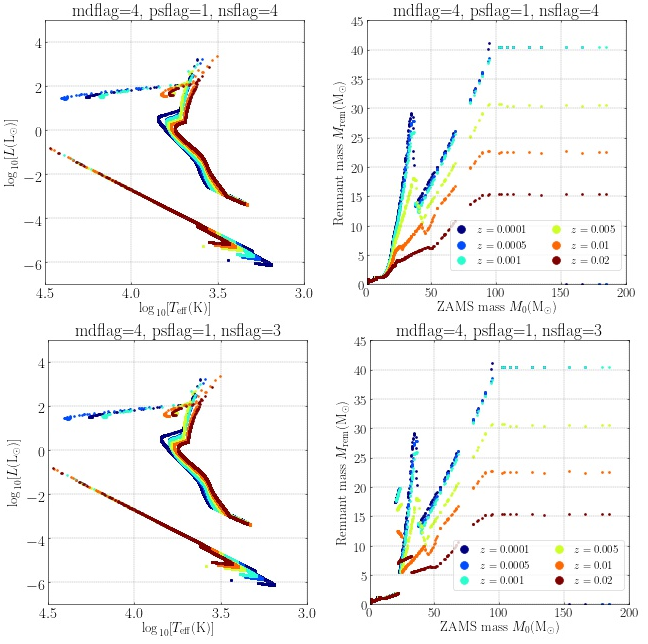
Figure 14: HRDs for the McLuster samples ($N=1.0\times 10^{5}$ single ZAMS stars) for all stars and the IFMRs of the compact objects depending on six different metallicities ranging from $Z$=0.0001 to Solar metallicity at $Z$=0.02. On top, the results for delayed SNe (nsflag=4) and on the bottom the results for the rapid SNe are shown (nsflag=3) (Fryer et al., 2012). The ZAMS stars suffer wind mass loss via mdflag=4 (no bi-stability jump) (Belczynski et al., 2010) and the (P)PISNe are set to psflag=1 from Belczynski et al. (2016).

We simulate a star sample made up of only single ZAMS stars of size $N=1.0\times 10^{5}$ up to an epoch=12000.0, so 12 Gyr. The IMF is a Kroupa (2001) IMF between (0.08-150.0)$\mathrm{M}_{\odot}$. We investigate a range of metallicities $Z$ for the two extremes of the core-collapse SNe paradigm, the rapid nsflag=3 and the delayed nsflag=4 SNe (Fryer et al., 2012). The ZAMS stars suffer wind mass loss via mdflag=4, i.e. we ignore the bi-stability jump (Belczynski et al., 2010) (and the Reimer’s mass loss coefficient set to neta=0.477 (McDonald & Zijlstra, 2015)), and the (P)PISNe are set to psflag=1 from Belczynski et al. (2016). The specific time-steps pts1, pts2, pts3 follow suggestions from Banerjee et al. (2020). The random seeds in McLuster are the same (seedmc=19640916) for all samples and therefore, we are evolving the identical ZAMS sample each time.
The results are shown in Fig.14 for the delayed SNe on the top and the rapid SNe on the bottom. For both the remnant masses decrease continuously for increasing metallicity. This is mainly due to the fact that at lower metallicities the mass loss from the stars before undergoing a core-collapse SNe (or another evolutionary process that leads to a compact object) is lower than at large metallicities (Vink et al., 2001; Vink & de Koter, 2005). At metallicities as large as $Z$=0.005, the mass loss is so large and the resulting BH mass so low that the (P)PISNe are not triggered at all, see Fig.15. The results mirror those from Banerjee et al. (2020) and therefore the implementations in Nbody7, which confirms an accurate implementation of Levels A, B and C in McLuster.

B.1.2 (P)PISNe and metallicity dependence

We simulate a star sample made up of only single ZAMS stars of size $N=2.5\times 10^{4}$ up to an epoch=12000.0, so 12 Gyr. The IMF is a Kroupa (2001) IMF between (30.0-500.0)$\mathrm{M}_{\odot}$. We note that this is a large extrapolation of what should be considered safe in the original SSE & BSE (Hurley et al., 2000, 2002). But these masses are reached already in dense simulations, see Di Carlo et al. (2021); Rizzuto et al. (2021b); Rizzuto et al. (2021a); Arca-Sedda et al. (2021). We need the implementations in the SSE&BSE from Tanikawa et al. (2020, 2021); Hijikawa et al. (2021) to properly models these stars in McLuster in the future. We investigate a range of metallicities $Z$ (0.0001-0.02). The ZAMS stars suffer wind mass loss via mdflag=4, i.e. we ignore the bi-stability jump (Belczynski et al., 2010) (and the Reimer’s mass loss coefficient set to neta=0.477 (McDonald & Zijlstra, 2015)), and we subject the stars to the rapid SNe core-collapse presciption (Fryer et al., 2012). The specific time-steps pts1, pts2, pts3 follow suggestions from Banerjee et al. (2020). We investigate a range of metallicities $Z$ for the available (P)PISNe recipes: psflag=1 (Belczynski et al., 2016), psflag=2 (Leung et al., 2019b; Leung et al., 2020b) and psflag=3 (Leung et al., 2019b; Leung et al., 2020b). The random seeds in McLuster are the same (seedmc=19640916) for all samples and therefore, we are evolving the identical ZAMS sample each time.
The results are shown in Fig.15. We see that the main difference between the three prescriptions is the onset of the (P)PISNe and the masses that result thereof. For low metallicities ($z<0.001$), the Leung et al. (2019b); Leung et al. (2020b) (P)PISNe produce high mass BHs for much larger ZAMS masses than the Belczynski et al. (2016) (P)PISNe. At metallicities as large as $Z$=0.005, the mass loss is so large and the resulting BH mass so low that the (P)PISNe are not triggered at all, see also Fig.14. Here, the remnant masses then coincide for all psflag ($z>0.005$). At large ZAMS and at the offset of the PISNe, the BH remnant masses are the same for psflag. Apart from initialising star cluster simulations with an IMF that is top-heavy and goes up to very large masses, e.g. Weatherford et al. (2021), these BH masses may be reached through initial stellar collisions and coalescence in primordial binaries (Kremer et al., 2020b). Alternatively, these may be reached dynamical through BH-BH mergers (Morawski et al., 2018, 2019; Di Carlo et al., 2019; Rizzuto et al., 2021b; Rizzuto et al., 2021a; Arca-Sedda et al., 2021).

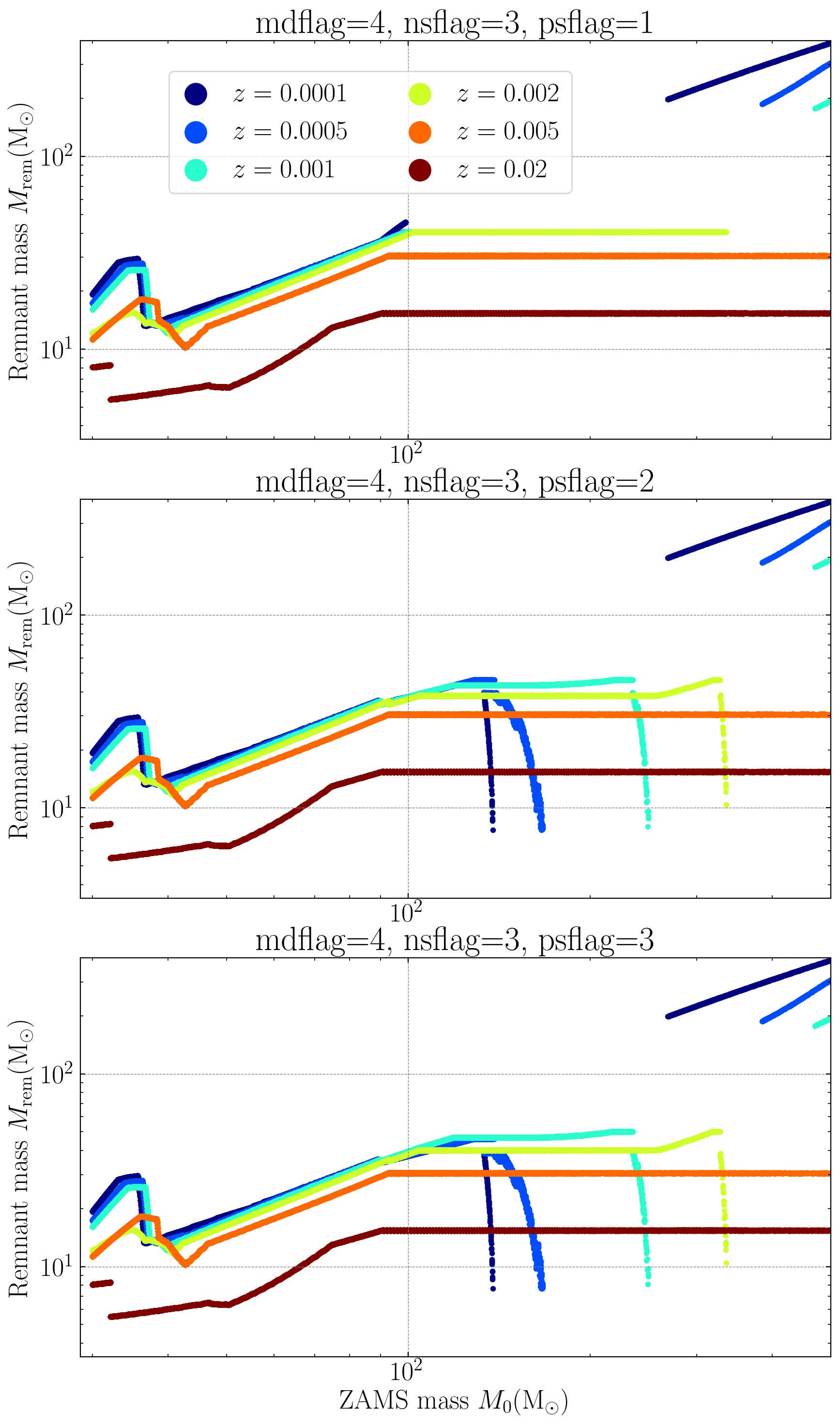
Figure 15: IFMRs of the BHs from the McLuster samples ($N=2.5\times 10^{4}$ single ZAMS stars) depending on six different metallicities ranging from $Z$=0.0001 to Solar metallicity at $Z$=0.02. Shown are the (P)PISNe recipes for psflag=1 on top (Belczynski et al., 2016), psflag=2 in the middle (Leung et al., 2019b; Leung et al., 2020b) and psflag=3 on the bottom (Leung et al., 2019b; Leung et al., 2020b). The ZAMS stars suffer wind mass loss via mdflag=4 (no bi-stability jump) (Belczynski et al., 2010) and the core-collapse SNe are rapid (Fryer et al., 2012).

References

- Aarseth (1985) Aarseth S. J., 1985, in Goodman J., Hut P., eds, Vol. 113, Dynamics of Star Clusters. pp 251–258
- Aarseth (1999a) Aarseth S. J., 1999a, CeMDA, 73, 127
- Aarseth (1999b) Aarseth S. J., 1999b, PASP, 111, 1333
- Aarseth (2003) Aarseth S. J., 2003, Gravitational N-Body Simulations
- Aarseth (2012) Aarseth S. J., 2012, MNRAS, 422, 841
- Aarseth & Lecar (1975) Aarseth S. J., Lecar M., 1975, ARAA, 13, 1
- Aarseth et al. (1974) Aarseth S. J., Henon M., Wielen R., 1974, AAP, 37, 183
- Aarseth et al. (2008) Aarseth S. J., Tout C. A., Mardling R. A., 2008, The Cambridge N-Body Lectures. Vol. 760, doi:10.1007/978-1-4020-8431-7,
- Aasi et al. (2015) Aasi J., et al., 2015, Classical and Quantum Gravity, 32, 115012
- Abbott et al. (2016) Abbott B. P., Abbott R., Abbott T. D., Abernathy M. R., Acernese F., et al. 2016, PhRvL, 116, 061102
- Abbott et al. (2017a) Abbott B. P., Abbott R., Abbott T. D., Acernese F., Ackley K., et al. 2017a, PhRvL, 119, 161101
- Abbott et al. (2017b) Abbott B. P., Abbott R., Abbott T. D., Acernese F., Ackley K., et al. 2017b, ApJL, 848, L12
- Abbott et al. (2018) Abbott B. P., et al., 2018, PRL, 121, 231103
- Abbott et al. (2019) Abbott B. P., Abbott R., Abbott T. D., Abraham S., Acernese F., et al. 2019, ApJL, 882, L24
- Abbott et al. (2020a) Abbott R., Abbott T. D., Abraham S., Acernese F., Ackley K., et al. 2020a, PhRvL, 125, 101102
- Abbott et al. (2020b) Abbott R., Abbott T. D., Abraham S., Acernese F., Ackley K., et al. 2020b, ApJL, 896, L44
- Acernese et al. (2015) Acernese F., et al., 2015, Classical and Quantum Gravity, 32, 024001
- Agrawal et al. (2020) Agrawal P., Hurley J., Stevenson S., Szécsi D., Flynn C., 2020, MNRAS, 497, 4549
- Ahmad & Cohen (1973) Ahmad A., Cohen L., 1973, Journal of Computational Physics, 12, 389
- Amaro-Seoane et al. (2010) Amaro-Seoane P., Eichhorn C., Porter E. K., Spurzem R., 2010, MNRAS, 401, 2268
- Antonini & Gieles (2020) Antonini F., Gieles M., 2020, PRD, 102, 123016
- Arca Sedda (2020) Arca Sedda M., 2020, CmPhy, 3, 43
- Arca Sedda et al. (2019) Arca Sedda M., Askar A., Giersz M., 2019, arXiv, p. arXiv:1905.00902
- Arca Sedda et al. (2020) Arca Sedda M., Berry C. P. L., Jani K., Amaro-Seoane P., Auclair P., et al. 2020, CQGra, 37, 215011
- Arca-Sedda et al. (2021) Arca-Sedda M., Rizzuto F. P., Naab T., Ostriker J., Giersz M., Spurzem R., 2021, ApJ, 920, 128
- Askar et al. (2017) Askar A., Szkudlarek M., Gondek-Rosińska D., Giersz M., Bulik T., 2017, MNRAS, 464, L36
- Baker et al. (2007) Baker J. G., Boggs W. D., Centrella J., Kelly B. J., McWilliams S. T., et al. 2007, ApJ, 668, 1140
- Baker et al. (2008) Baker J. G., Boggs W. D., Centrella J., Kelly B. J., McWilliams S. T., et al. 2008, PhRvD, 78, 044046
- Banerjee (2018) Banerjee S., 2018, MNRAS, 473, 909
- Banerjee (2021a) Banerjee S., 2021a, arXiv e-prints, p. arXiv:2109.14612
- Banerjee (2021b) Banerjee S., 2021b, MNRAS, 500, 3002
- Banerjee et al. (2020) Banerjee S., Belczynski K., Fryer C. L., Berczik P., Hurley J. R., et al. 2020, A&A, 639, A41
- Barniske et al. (2008) Barniske A., Oskinova L. M., Hamann W. R., 2008, A&A, 486, 971
- Baumgardt (2001) Baumgardt H., 2001, MNRAS, 325, 1323
- Baumgardt & Hilker (2018) Baumgardt H., Hilker M., 2018, MNRAS, 478, 1520
- Baumgardt & Makino (2003) Baumgardt H., Makino J., 2003, MNRAS, 340, 227
- Baumgardt et al. (2008) Baumgardt H., De Marchi G., Kroupa P., 2008, ApJ, 685, 247
- Baym et al. (2018) Baym G., Hatsuda T., Kojo T., Powell P. D., Song Y., et al. 2018, RPPh, 81, 056902
- Baym et al. (2019) Baym G., Furusawa S., Hatsuda T., Kojo T., Togashi H., 2019, ApJ, 885, 42
- Belczynski & Banerjee (2020) Belczynski K., Banerjee S., 2020, A&A, 640, L20
- Belczynski et al. (2002) Belczynski K., Kalogera V., Bulik T., 2002, ApJ, 572, 407
- Belczynski et al. (2008) Belczynski K., Kalogera V., Rasio F. A., Taam R. E., Zezas A., et al. 2008, ApJS, 174, 223
- Belczynski et al. (2010) Belczynski K., Bulik T., Fryer C. L., Ruiter A., Valsecchi F., et al. 2010, ApJ, 714, 1217
- Belczynski et al. (2016) Belczynski K., Heger A., Gladysz W., Ruiter A. J., Woosley S., et al. 2016, A&A, 594, A97
- Belczynski et al. (2020) Belczynski K., Klencki J., Fields C. E., Olejak A., Berti E., et al. 2020, A&A, 636, A104
- Belloni et al. (2017a) Belloni D., Giersz M., Rocha-Pinto H. J., Leigh N. W. C., Askar A., 2017a, MNRAS, 464, 4077
- Belloni et al. (2017b) Belloni D., Zorotovic M., Schreiber M. R., Leigh N. W. C., Giersz M., et al. 2017b, MNRAS, 468, 2429
- Belloni et al. (2017c) Belloni D., Askar A., Giersz M., Kroupa P., Rocha-Pinto H. J., 2017c, MNRAS, 471, 2812
- Belloni et al. (2018a) Belloni D., Kroupa P., Rocha-Pinto H. J., Giersz M., 2018a, MNRAS, 474, 3740
- Belloni et al. (2018b) Belloni D., Schreiber M. R., Zorotovic M., Iłkiewicz K., Hurley J. R., et al. 2018b, MNRAS, 478, 5626
- Belloni et al. (2019) Belloni D., Giersz M., Rivera Sandoval L. E., Askar A., Ciecielåg P., 2019, MNRAS, 483, 315
- Belloni et al. (2020a) Belloni D., Schreiber M. R., Pala A. F., Gänsicke B. T., Zorotovic M., et al. 2020a, MNRAS, 491, 5717
- Belloni et al. (2020b) Belloni D., Mikołajewska J., Iłkiewicz K., Schreiber M. R., Giersz M., et al. 2020b, MNRAS, 496, 3436
- Benacquista & Downing (2013) Benacquista M. J., Downing J. M. B., 2013, LRR, 16, 4
- Bestenlehner et al. (2020) Bestenlehner J. M., Crowther P. A., Caballero-Nieves S. M., Schneider F. R. N., Simón-Díaz S., et al. 2020, MNRAS, 499, 1918
- Bianchini et al. (2013) Bianchini P., Varri A. L., Bertin G., Zocchi A., 2013, ApJ, 772, 67
- Bianchini et al. (2018) Bianchini P., van der Marel R. P., del Pino A., Watkins L. L., Bellini A., et al. 2018, MNRAS, 481, 2125
- Bianchini et al. (2019) Bianchini P., Ibata R., Famaey B., 2019, ApJL, 887, L12
- Blanchet (2014) Blanchet L., 2014, LRR, 17, 2
- Bondi & Hoyle (1944) Bondi H., Hoyle F., 1944, MNRAS, 104, 273
- Boshkayev et al. (2013) Boshkayev K., Rueda J. A., Ruffini R., Siutsou I., 2013, ApJ, 762, 117
- Breivik et al. (2020) Breivik K., Coughlin S., Zevin M., Rodriguez C. L., Kremer K., et al. 2020, ApJ, 898, 71
- Brem et al. (2013) Brem P., Amaro-Seoane P., Spurzem R., 2013, MNRAS, 434, 2999
- Burrows & Hayes (1996) Burrows A., Hayes J., 1996, PhRvL, 76, 352
- Camacho et al. (2014) Camacho J., Torres S., García-Berro E., Zorotovic M., Schreiber M. R., et al. 2014, A&A, 566, A86
- Cameron & Mock (1967) Cameron A. G. W., Mock M., 1967, Natur, 215, 464
- Campanelli et al. (2007) Campanelli M., Lousto C., Zlochower Y., Merritt D., 2007, ApJL, 659, L5
- Cantat-Gaudin et al. (2014) Cantat-Gaudin T., et al., 2014, AAP, 569, A17
- Chattopadhyay et al. (2020) Chattopadhyay D., Stevenson S., Hurley J. R., Rossi L. J., Flynn C., 2020, MNRAS, 494, 1587
- Chattopadhyay et al. (2021) Chattopadhyay D., Stevenson S., Hurley J. R., Bailes M., Broekgaarden F., 2021, MNRAS, 504, 3682
- Chen et al. (2015) Chen Y., Bressan A., Girardi L., Marigo P., Kong X., et al. 2015, MNRAS, 452, 1068
- Claeys et al. (2014) Claeys J. S. W., Pols O. R., Izzard R. G., Vink J., Verbunt F. W. M., 2014, A&A, 563, A83
- Clark (1975) Clark G. W., 1975, ApJL, 199, L143
- Cohn (1979) Cohn H., 1979, ApJ, 234, 1036
- Cojocaru et al. (2017) Cojocaru R., Rebassa-Mansergas A., Torres S., García-Berro E., 2017, MNRAS, 470, 1442
- De et al. (2020) De S., MacLeod M., Everson R. W., Antoni A., Mandel I., et al. 2020, ApJ, 897, 130
- Decin (2020) Decin L., 2020, arXiv e-prints, p. arXiv:2011.13472
- Dewi & Tauris (2000) Dewi J. D. M., Tauris T. M., 2000, A&A, 360, 1043
- Di Carlo et al. (2019) Di Carlo U. N., Giacobbo N., Mapelli M., Pasquato M., Spera M., et al. 2019, MNRAS, 487, 2947
- Di Carlo et al. (2020a) Di Carlo U. N., Mapelli M., Bouffanais Y., Giacobbo N., Santoliquido F., et al. 2020a, MNRAS, 497, 1043
- Di Carlo et al. (2020b) Di Carlo U. N., Mapelli M., Giacobbo N., Spera M., Bouffanais Y., et al. 2020b, MNRAS, 498, 495
- Di Carlo et al. (2021) Di Carlo U. N., Mapelli M., Pasquato M., Rastello S., Ballone A., et al. 2021, arXiv, p. arXiv:2105.01085
- Downing (2012) Downing J. M. B., 2012, MNRAS, 425, 2234
- Downing et al. (2010) Downing J. M. B., Benacquista M. J., Giersz M., Spurzem R., 2010, MNRAS, 407, 1946
- Downing et al. (2011) Downing J. M. B., Benacquista M. J., Giersz M., Spurzem R., 2011, MNRAS, 416, 133
- Doyle et al. (2019) Doyle T. F., Shara M. M., Lessing A. M., Zurek D., 2019, ApJ, 874, 65
- Drozda et al. (2020) Drozda P., Belczynski K., O’Shaughnessy R., Bulik T., Fryer C. L., 2020, arXiv, p. arXiv:2009.06655
- Duquennoy & Mayor (1991) Duquennoy A., Mayor M., 1991, A&A, 500, 337
- Eggenberger et al. (2008) Eggenberger P., Meynet G., Maeder A., Hirschi R., Charbonnel C., et al. 2008, Ap&SS, 316, 43
- Eggleton (1971) Eggleton P. P., 1971, MNRAS, 151, 351
- Eggleton (1972) Eggleton P. P., 1972, MNRAS, 156, 361
- Eggleton (1973) Eggleton P. P., 1973, MNRAS, 163, 279
- Eggleton et al. (1973) Eggleton P. P., Faulkner J., Flannery B. P., 1973, A&A, 23, 325
- Einsel & Spurzem (1999) Einsel C., Spurzem R., 1999, MNRAS, 302, 81
- Ekström et al. (2012) Ekström S., Georgy C., Eggenberger P., Meynet G., Mowlavi N., et al. 2012, A&A, 537, A146
- Eldridge & Tout (2004) Eldridge J. J., Tout C. A., 2004, MNRAS, 353, 87
- Elson et al. (1987) Elson R. A. W., Fall S. M., Freeman K. C., 1987, ApJ, 323, 54
- Ernst et al. (2007) Ernst A., Glaschke P., Fiestas J., Just A., Spurzem R., 2007, MNRAS, 377, 465
- Everson et al. (2020) Everson R. W., MacLeod M., De S., Macias P., Ramirez-Ruiz E., 2020, ApJ, 899, 77
- Faye et al. (2006) Faye G., Blanchet L., Buonanno A., 2006, PhRvD, 74, 104033
- Fellhauer et al. (2003) Fellhauer M., Lin D. N. C., Bolte M., Aarseth S. J., Williams K. A., 2003, ApJL, 595, L53
- Fiestas & Spurzem (2010) Fiestas J., Spurzem R., 2010, MNRAS, 405, 194
- Fragione & Banerjee (2020) Fragione G., Banerjee S., 2020, ApJL, 901, L16
- Fregeau et al. (2004) Fregeau J. M., Cheung P., Portegies Zwart S. F., Rasio F. A., 2004, MNRAS, 352, 1
- Fryer (2004) Fryer C. L., 2004, ApJ, 601, L175
- Fryer & Kalogera (1997) Fryer C., Kalogera V., 1997, ApJ, 489, 244
- Fryer & Kusenko (2006) Fryer C. L., Kusenko A., 2006, ApJS, 163, 335
- Fryer & Young (2007) Fryer C. L., Young P. A., 2007, ApJ, 659, 1438
- Fryer et al. (2012) Fryer C. L., Belczynski K., Wiktorowicz G., Dominik M., Kalogera V., et al. 2012, ApJ, 749, 91
- Fukushige & Heggie (2000) Fukushige T., Heggie D. C., 2000, MNRAS, 318, 753
- Fuller & Ma (2019) Fuller J., Ma L., 2019, ApJL, 881, L1
- Fuller et al. (2003) Fuller G. M., Kusenko A., Mocioiu I., Pascoli S., 2003, PhRvD, 68, 103002
- Fuller et al. (2019) Fuller J., Piro A. L., Jermyn A. S., 2019, MNRAS, 485, 3661
- Geller et al. (2019) Geller A. M., Leigh N. W. C., Giersz M., Kremer K., Rasio F. A., 2019, ApJ, 872, 165
- Gessner & Janka (2018) Gessner A., Janka H.-T., 2018, ApJ, 865, 61
- Giacobbo & Mapelli (2018) Giacobbo N., Mapelli M., 2018, MNRAS, 480, 2011
- Giacobbo & Mapelli (2019) Giacobbo N., Mapelli M., 2019, MNRAS, 486, 2494
- Giacobbo et al. (2018) Giacobbo N., Mapelli M., Spera M., 2018, MNRAS, 474, 2959
- Giersz (1998) Giersz M., 1998, MNRAS, 298, 1239
- Giersz (2001) Giersz M., 2001, MNRAS, 324, 218
- Giersz & Heggie (1994) Giersz M., Heggie D. C., 1994, MNRAS, 268, 257
- Giersz et al. (2008) Giersz M., Heggie D. C., Hurley J. R., 2008, MNRAS, 388, 429
- Giersz et al. (2013) Giersz M., Heggie D. C., Hurley J. R., Hypki A., 2013, MNRAS, 431, 2184
- Giersz et al. (2014) Giersz M., Leigh N., Marks M., Hypki A., Askar A., 2014, arXiv, p. arXiv:1411.7603
- Giersz et al. (2015) Giersz M., Leigh N., Hypki A., Lützgendorf N., Askar A., 2015, MNRAS, 454, 3150
- Giersz et al. (2016) Giersz M., Leigh N., Hypki A., Askar A., Lützgendorf N., 2016, MmSAI, 87, 555
- Giesers et al. (2018) Giesers B., et al., 2018, MNRAS, 475, L15
- Giesers et al. (2019) Giesers B., et al., 2019, AAP, 632, A3
- Goodwin & Whitworth (2004) Goodwin S. P., Whitworth A. P., 2004, A&A, 413, 929
- Gräfener & Hamann (2008) Gräfener G., Hamann W. R., 2008, A&A, 482, 945
- Gratton et al. (2012) Gratton R. G., Carretta E., Bragaglia A., 2012, AAPR, 20, 50
- Hamann & Koesterke (1998) Hamann W. R., Koesterke L., 1998, A&A, 335, 1003
- Han et al. (1995) Han Z., Podsiadlowski P., Eggleton P. P., 1995, MNRAS, 272, 800
- Hansen & Phinney (1997) Hansen B. M. S., Phinney E. S., 1997, MNRAS, 291, 569
- Harris (1996) Harris W. E., 1996, AJ, 112, 1487
- Heggie (1975) Heggie D. C., 1975, MNRAS, 173, 729
- Heggie & Giersz (2014) Heggie D. C., Giersz M., 2014, MNRAS, 439, 2459
- Hellström & Mikkola (2010) Hellström C., Mikkola S., 2010, Celestial Mechanics and Dynamical Astronomy, 106, 143
- Hénon (1975) Hénon M., 1975, in Hayli A., ed., Vol. 69, Dynamics of the Solar Systems. p. 133
- Higgins & Vink (2019) Higgins E. R., Vink J. S., 2019, AAP, 622, A50
- Higgins et al. (2021) Higgins E. R., Sander A. A. C., Vink J. S., Hirschi R., 2021, MNRAS, 505, 4874
- Hijikawa et al. (2021) Hijikawa K., Tanikawa A., Kinugawa T., Yoshida T., Umeda H., 2021, MNRAS.tmp,
- Hillier et al. (2001) Hillier D. J., Davidson K., Ishibashi K., Gull T., 2001, ApJ, 553, 837
- Hobbs et al. (2005) Hobbs G., Lorimer D. R., Lyne A. G., Kramer M., 2005, MNRAS, 360, 974
- Hong et al. (2013) Hong J., Kim E., Lee H. M., Spurzem R., 2013, MNRAS, 430, 2960
- Hong et al. (2018) Hong J., Vesperini E., Askar A., Giersz M., Szkudlarek M., et al. 2018, MNRAS, 480, 5645
- Hong et al. (2020a) Hong J., Vesperini E., Askar A., Giersz M., Szkudlarek M., et al. 2020a, MNRAS, 491, 5793
- Hong et al. (2020b) Hong J., Askar A., Giersz M., Hypki A., Yoon S.-J., 2020b, MNRAS, 498, 4287
- Huang & Koposov (2021) Huang K.-W., Koposov S. E., 2021, MNRAS, 500, 986
- Hughes (2009) Hughes S. A., 2009, ARA&A, 47, 107
- Humphreys & Davidson (1979) Humphreys R. M., Davidson K., 1979, ApJ, 232, 409
- Humphreys & Davidson (1994) Humphreys R. M., Davidson K., 1994, PASP, 106, 1025
- Hurley & Shara (2003) Hurley J. R., Shara M. M., 2003, ApJ, 589, 179
- Hurley et al. (2000) Hurley J. R., Pols O. R., Tout C. A., 2000, MNRAS, 315, 543
- Hurley et al. (2002) Hurley J. R., Tout C. A., Pols O. R., 2002, MNRAS, 329, 897
- Hurley et al. (2013a) Hurley J. R., Tout C. A., Pols O. R., 2013a, BSE: Binary Star Evolution (ascl:1303.014)
- Hurley et al. (2013b) Hurley J. R., Pols O. R., Tout C. A., 2013b, SSE: Single Star Evolution (ascl:1303.015)
- Husser et al. (2016) Husser T.-O., Kamann S., Dreizler S., Wendt M., Wulff N., et al. 2016, A&A, 588, A148
- Hut et al. (1995) Hut P., Makino J., McMillan S., 1995, ApJL, 443, L93
- Hypki & Giersz (2013) Hypki A., Giersz M., 2013, MNRAS, 429, 1221
- Ivanova (2016) Ivanova N., 2016, in Meiron Y., Li S., Liu F. K., Spurzem R., eds, Vol. 312, Star Clusters and Black Holes in Galaxies across Cosmic Time. pp 203–212 (arXiv:1706.07578), doi:10.1017/S1743921315007826
- Ivanova et al. (2008) Ivanova N., Heinke C. O., Rasio F. A., Belczynski K., Fregeau J. M., 2008, MNRAS, 386, 553
- Ivanova et al. (2013) Ivanova N., Justham S., Chen X., De Marco O., Fryer C. L., et al. 2013, A&ARv, 21, 59
- Ivanova et al. (2020) Ivanova N., Justham S., Ricker P., 2020, Common Envelope Evolution. 2514-3433, IOP Publishing, doi:10.1088/2514-3433/abb6f0, http://dx.doi.org/10.1088/2514-3433/abb6f0
- Jordan et al. (2012) Jordan George C. I., Perets H. B., Fisher R. T., van Rossum D. R., 2012, ApJL, 761, L23
- Kamann et al. (2018a) Kamann S., Husser T. O., Dreizler S., Emsellem E., Weilbacher P. M., et al. 2018a, MNRAS, 473, 5591
- Kamann et al. (2018b) Kamann S., Bastian N., Husser T. O., Martocchia S., Usher C., et al. 2018b, MNRAS, 480, 1689
- Kamann et al. (2020a) Kamann S., Bastian N., Gossage S., Baade D., Cabrera-Ziri I., et al. 2020a, MNRAS, 492, 2177
- Kamann et al. (2020b) Kamann S., Giesers B., Bastian N., Brinchmann J., Dreizler S., et al. 2020b, A&A, 635, A65
- Kerr (1963) Kerr R. P., 1963, PhRvL, 11, 237
- Khalisi et al. (2007) Khalisi E., Amaro-Seoane P., Spurzem R., 2007, MNRAS, 374, 703
- Kiel et al. (2008) Kiel P. D., Hurley J. R., Bailes M., Murray J. R., 2008, MNRAS, 388, 393
- Kiel et al. (2010) Kiel P. D., Hurley J. R., Bailes M., 2010, MNRAS, 406, 656
- Kim et al. (2008) Kim E., Yoon I., Lee H. M., Spurzem R., 2008, MNRAS, 383, 2
- Kiminki et al. (2012) Kiminki D. C., Kobulnicky H. A., Ewing I., Bagley Kiminki M. M., Lundquist M., et al. 2012, ApJ, 747, 41
- King (1962) King I., 1962, AJ, 67, 471
- King (1966) King I. R., 1966, AJ, 71, 64
- King & Kolb (1995) King A. R., Kolb U., 1995, ApJ, 439, 330
- Knigge (2006) Knigge C., 2006, MNRAS, 373, 484
- Knigge et al. (2011) Knigge C., Baraffe I., Patterson J., 2011, ApJS, 194, 28
- Kobulnicky & Fryer (2007) Kobulnicky H. A., Fryer C. L., 2007, ApJ, 670, 747
- Kobulnicky et al. (2014) Kobulnicky H. A., Kiminki D. C., Lundquist M. J., Burke J., Chapman J., et al. 2014, ApJS, 213, 34
- Kouwenhoven et al. (2007) Kouwenhoven M. B. N., Brown A. G. A., Portegies Zwart S. F., Kaper L., 2007, A&A, 474, 77
- Kremer et al. (2018) Kremer K., Chatterjee S., Rodriguez C. L., Rasio F. A., 2018, ApJ, 852, 29
- Kremer et al. (2019) Kremer K., Rodriguez C. L., Amaro-Seoane P., Breivik K., Chatterjee S., et al. 2019, PhRvD, 99, 063003
- Kremer et al. (2020a) Kremer K., Ye C. S., Rui N. Z., Weatherford N. C., Chatterjee S., et al. 2020a, ApJS, 247, 48
- Kremer et al. (2020b) Kremer K., Spera M., Becker D., Chatterjee S., Di Carlo U. N., et al. 2020b, ApJ, 903, 45
- Kremer et al. (2021) Kremer K., Rui N. Z., Weatherford N. C., Chatterjee S., Fragione G., et al. 2021, arXiv, p. arXiv:2104.11751
- Kroupa (1995a) Kroupa P., 1995a, MNRAS, 277, 1491
- Kroupa (1995b) Kroupa P., 1995b, MNRAS, 277, 1507
- Kroupa (2001) Kroupa P., 2001, MNRAS, 322, 231
- Kroupa (2008) Kroupa P., 2008, Initial Conditions for Star Clusters. p. 181, doi:10.1007/978-1-4020-8431-7_8
- Kroupa (2009) Kroupa P., 2009, in Andersen J., Nordströara m B., Bland-Hawthorn J., eds, Vol. 254, The Galaxy Disk in Cosmological Context. pp 209–220 (arXiv:0810.4143), doi:10.1017/S1743921308027610
- Kroupa et al. (1993) Kroupa P., Tout C. A., Gilmore G., 1993, MNRAS, 262, 545
- Krumholz et al. (2019) Krumholz M. R., McKee C. F., Bland-Hawthorn J., 2019, ARA&A, 57, 227
- Kudritzki & Reimers (1978) Kudritzki R. P., Reimers D., 1978, A&A, 70, 227
- Kudritzki et al. (1989) Kudritzki R. P., Pauldrach A., Puls J., Abbott D. C., 1989, A&A, 219, 205
- Kuepper et al. (2011) Kuepper A. H. W., Maschberger T., Kroupa P., Baumgardt H., 2011, McLuster: A Tool to Make a Star Cluster (ascl:1107.015)
- Kuhn et al. (2019) Kuhn M. A., Hillenbrand L. A., Sills A., Feigelson E. D., Getman K. V., 2019, ApJ, 870, 32
- Kupi et al. (2006) Kupi G., Amaro-Seoane P., Spurzem R., 2006, MNRAS, 371, L45
- Kuranov & Postnov (2006) Kuranov A. G., Postnov K. A., 2006, AstL, 32, 393
- Lada & Lada (2003) Lada C. J., Lada E. A., 2003, ARA&A, 41, 57
- Langer et al. (2020) Langer N., Schürmann C., Stoll K., Marchant P., Lennon D. J., et al. 2020, A&A, 638, A39
- Larson (1970a) Larson R. B., 1970a, MNRAS, 147, 323
- Larson (1970b) Larson R. B., 1970b, MNRAS, 150, 93
- Latour et al. (2019) Latour M., Husser T. O., Giesers B., Kamann S., Göttgens F., et al. 2019, A&A, 631, A14
- Lattimer & Prakash (2004) Lattimer J. M., Prakash M., 2004, Sci, 304, 536
- Leigh et al. (2015) Leigh N. W. C., Giersz M., Marks M., Webb J. J., Hypki A., et al. 2015, MNRAS, 446, 226
- Leung et al. (2019a) Leung S.-C., Zha S., Chu M.-C., Lin L.-M., Nomoto K., 2019a, ApJ, 884, 9
- Leung et al. (2019b) Leung S.-C., Nomoto K., Blinnikov S., 2019b, ApJ, 887, 72
- Leung et al. (2020a) Leung S.-C., Nomoto K., Suzuki T., 2020a, ApJ, 889, 34
- Leung et al. (2020b) Leung S.-C., Blinnikov S., Ishidoshiro K., Kozlov A., Nomoto K., 2020b, ApJ, 889, 75
- Leung et al. (2020c) Leung S.-C., Blinnikov S., Nomoto K., Baklanov P., Sorokina E., et al. 2020c, ApJ, 903, 66
- Leveque et al. (2021) Leveque A., Giersz M., Paolillo M., 2021, MNRAS, 501, 5212
- Linares (2018) Linares M., 2018, in 42nd COSPAR Scientific Assembly. pp E1.3–27–18
- Madrid et al. (2017) Madrid J. P., Leigh N. W. C., Hurley J. R., Giersz M., 2017, MNRAS, 470, 1729
- Makino (1991) Makino J., 1991, ApJ, 369, 200
- Makino (1999) Makino J., 1999, Journal of Computational Physics, 151, 910
- Manchester et al. (2005) Manchester R. N., Hobbs G. B., Teoh A., Hobbs M., 2005, AJ, 129, 1993
- Mapelli et al. (2020a) Mapelli M., Santoliquido F., Bouffanais Y., Arca Sedda M., Giacobbo N., et al. 2020a, arXiv, p. arXiv:2007.15022
- Mapelli et al. (2020b) Mapelli M., Spera M., Montanari E., Limongi M., Chieffi A., et al. 2020b, ApJ, 888, 76
- Mardling & Aarseth (2001) Mardling R. A., Aarseth S. J., 2001, MNRAS, 321, 398
- Martinazzi et al. (2014) Martinazzi E., Pieres A., Kepler S. O., Costa J. E. S., Bonatto C., et al. 2014, MNRAS, 442, 3105
- Mazzali et al. (2007) Mazzali P. A., Röpke F. K., Benetti S., Hillebrandt W., 2007, Sci, 315, 825
- McDonald & Zijlstra (2015) McDonald I., Zijlstra A. A., 2015, MNRAS, 448, 502
- McMillan (1986) McMillan S. L. W., 1986, The Vectorization of Small-N Integrators. p. 156, doi:10.1007/BFb0116406
- Meakin & Arnett (2006) Meakin C. A., Arnett D., 2006, ApJL, 637, L53
- Meakin & Arnett (2007) Meakin C. A., Arnett D., 2007, ApJ, 665, 690
- Merritt (2015) Merritt D., 2015, ApJ, 804, 52
- Mestel (1952) Mestel L., 1952, MNRAS, 112, 583
- Mikkola & Aarseth (1993) Mikkola S., Aarseth S. J., 1993, Celestial Mechanics and Dynamical Astronomy, 57, 439
- Mikkola & Aarseth (1998) Mikkola S., Aarseth S. J., 1998, NA, 3, 309
- Mikkola & Merritt (2008) Mikkola S., Merritt D., 2008, AJ, 135, 2398
- Mikkola & Tanikawa (1999a) Mikkola S., Tanikawa K., 1999a, Celestial Mechanics and Dynamical Astronomy, 74, 287
- Mikkola & Tanikawa (1999b) Mikkola S., Tanikawa K., 1999b, MNRAS, 310, 745
- Milone et al. (2012) Milone A. P., Piotto G., Bedin L. R., King I. R., Anderson J., et al. 2012, ApJ, 744, 58
- Moe & Di Stefano (2017) Moe M., Di Stefano R., 2017, ApJS, 230, 15
- Morawski et al. (2018) Morawski J., Giersz M., Askar A., Belczynski K., 2018, MNRAS, 481, 2168
- Morawski et al. (2019) Morawski J., Giersz M., Askar A., Belczynski K., 2019, MNRAS, 486, 3402
- Nieuwenhuijzen & de Jager (1990) Nieuwenhuijzen H., de Jager C., 1990, A&A, 231, 134
- Nitadori & Aarseth (2012) Nitadori K., Aarseth S. J., 2012, MNRAS, 424, 545
- Nomoto (1984) Nomoto K., 1984, ApJ, 277, 791
- Nomoto (1987) Nomoto K., 1987, ApJ, 322, 206
- Nomoto & Kondo (1991) Nomoto K., Kondo Y., 1991, ApJL, 367, L19
- Oh et al. (2015) Oh S., Kroupa P., Pflamm-Altenburg J., 2015, ApJ, 805, 92
- Olejak et al. (2020) Olejak A., Belczynski K., Bulik T., Sobolewska M., 2020, A&A, 638, A94
- Ott (2009) Ott C. D., 2009, Classical and Quantum Gravity, 26, 204015
- Paczynski (1976) Paczynski B., 1976, in Eggleton P., Mitton S., Whelan J., eds, Vol. 73, Structure and Evolution of Close Binary Systems. p. 75
- Panamarev et al. (2019) Panamarev T., Just A., Spurzem R., Berczik P., Wang L., et al. 2019, MNRAS, 484, 3279
- Paxton et al. (2011) Paxton B., Bildsten L., Dotter A., Herwig F., Lesaffre P., et al. 2011, ApJS, 192, 3
- Paxton et al. (2015) Paxton B., Marchant P., Schwab J., Bauer E. B., Bildsten L., et al. 2015, ApJS, 220, 15
- Peters (1964) Peters P. C., 1964, PhRv, 136, 1224
- Peters & Mathews (1963) Peters P. C., Mathews J., 1963, PhRv, 131, 435
- Plummer (1911) Plummer H. C., 1911, MNRAS, 71, 460
- Podsiadlowski et al. (2004) Podsiadlowski P., Langer N., Poelarends A. J. T., Rappaport S., Heger A., et al. 2004, ApJ, 612, 1044
- Pols et al. (1995) Pols O. R., Tout C. A., Eggleton P. P., Han Z., 1995, MNRAS, 274, 964
- Portegies Zwart & McMillan (2002) Portegies Zwart S. F., McMillan S. L. W., 2002, ApJ, 576, 899
- Portegies Zwart et al. (2010) Portegies Zwart S. F., McMillan S. L. W., Gieles M., 2010, ARA&A, 48, 431
- Railton et al. (2014) Railton A. D., Tout C. A., Aarseth S. J., 2014, PASA, 31, e017
- Rantala et al. (2020) Rantala A., Pihajoki P., Mannerkoski M., Johansson P. H., Naab T., 2020, MNRAS, 492, 4131
- Rantala et al. (2021) Rantala A., Naab T., Springel V., 2021, MNRAS, 502, 5546
- Rappaport et al. (1983) Rappaport S., Verbunt F., Joss P. C., 1983, ApJ, 275, 713
- Rebassa-Mansergas et al. (2012) Rebassa-Mansergas A., Nebot Gómez-Morán A., Schreiber M. R., Gänsicke B. T., Schwope A., et al. 2012, MNRAS, 419, 806
- Reimers (1975) Reimers D., 1975, MSRSL, 8, 369
- Reina-Campos et al. (2019) Reina-Campos M., Kruijssen J. M. D., Pfeffer J. L., Bastian N., Crain R. A., 2019, MNRAS, 486, 5838
- Reina-Campos et al. (2020) Reina-Campos M., Hughes M. E., Kruijssen J. M. D., Pfeffer J. L., Bastian N., et al. 2020, MNRAS, 493, 3422
- Reina-Campos et al. (2021) Reina-Campos M., Trujillo-Gomez S., Deason A. J., Kruijssen J. M. D., Pfeffer J. L., et al. 2021, arXiv, p. arXiv:2106.07652
- Rezzolla et al. (2008) Rezzolla L., Barausse E., Dorband E. N., Pollney D., Reisswig C., et al. 2008, PhRvD, 78, 044002
- Ritter (1988) Ritter H., 1988, A&A, 202, 93
- Rizzuto et al. (2021a) Rizzuto F. P., Naab T., Spurzem R., Arca-Sedda M., Giersz M., Ostriker J. P., Banerjee S., 2021a, arXiv e-prints, p. arXiv:2108.11457
- Rizzuto et al. (2021b) Rizzuto F. P., Naab T., Spurzem R., Giersz M., Ostriker J. P., et al. 2021b, MNRAS, 501, 5257
- Sadavoy & Stahler (2017) Sadavoy S. I., Stahler S. W., 2017, MNRAS, 469, 3881
- Saio & Nomoto (1985) Saio H., Nomoto K., 1985, A&A, 150, L21
- Saio & Nomoto (2004) Saio H., Nomoto K., 2004, ApJ, 615, 444
- Sana & Evans (2011) Sana H., Evans C. J., 2011, in Neiner C., Wade G., Meynet G., Peters G., eds, Vol. 272, Active OB Stars: Structure, Evolution, Mass Loss, and Critical Limits. pp 474–485 (arXiv:1009.4197), doi:10.1017/S1743921311011124
- Sana et al. (2013) Sana H., de Mink S. E., de Koter A., Langer N., Evans C. J., et al. 2013, in Pugliese G., de Koter A., Wijburg M., eds, Astronomical Society of the Pacific Conference Series Vol. 470, 370 Years of Astronomy in Utrecht. p. 141 (arXiv:1211.4740)
- Sander & Vink (2020) Sander A. A. C., Vink J. S., 2020, MNRAS, 499, 873
- Sander et al. (2020) Sander A. A. C., Vink J. S., Hamann W. R., 2020, MNRAS, 491, 4406
- Santoliquido et al. (2020) Santoliquido F., Mapelli M., Bouffanais Y., Giacobbo N., Di Carlo U. N., et al. 2020, ApJ, 898, 152
- Scheck et al. (2004) Scheck L., Plewa T., Janka H. T., Kifonidis K., Müller E., 2004, PhRvL, 92, 011103
- Scheck et al. (2008) Scheck L., Janka H. T., Foglizzo T., Kifonidis K., 2008, A&A, 477, 931
- Schneider et al. (2021) Schneider F. R. N., Podsiadlowski P., Müller B., 2021, A&A, 645, A5
- Schödel et al. (2014) Schödel R., Feldmeier A., Neumayer N., Meyer L., Yelda S., 2014, CQGra, 31, 244007
- Schreiber et al. (2010) Schreiber M. R., Gänsicke B. T., Rebassa-Mansergas A., Nebot Gomez-Moran A., Southworth J., et al. 2010, A&A, 513, L7
- Schreiber et al. (2016) Schreiber M. R., Zorotovic M., Wijnen T. P. G., 2016, MNRAS, 455, L16
- Schröder & Cuntz (2005) Schröder K. P., Cuntz M., 2005, ApJL, 630, L73
- Shu et al. (2021) Shu Q., Pang X., Flammini Dotti F., Kouwenhoven M. B. N., Arca Sedda M., et al. 2021, ApJS, 253, 14
- Spera & Mapelli (2017) Spera M., Mapelli M., 2017, MNRAS, 470, 4739
- Spera et al. (2015) Spera M., Mapelli M., Bressan A., 2015, MNRAS, 451, 4086
- Spera et al. (2019) Spera M., Mapelli M., Giacobbo N., Trani A. A., Bressan A., et al. 2019, MNRAS, 485, 889
- Spruit (2002) Spruit H. C., 2002, AAP, 381, 923
- Spurzem (1999) Spurzem R., 1999, Journal of Computational and Applied Mathematics, 109, 407
- Spurzem (2001) Spurzem R., 2001, in Deiters S., Fuchs B., Just A., Spurzem R., Wielen R., eds, Astronomical Society of the Pacific Conference Series Vol. 228, Dynamics of Star Clusters and the Milky Way. p. 75
- Stevenson et al. (2017a) Stevenson S., Vigna-Gómez A., Mandel I., Barrett J. W., Neijssel C. J., et al. 2017a, NatCo, 8, 14906
- Stevenson et al. (2017b) Stevenson S., Berry C. P. L., Mandel I., 2017b, MNRAS, 471, 2801
- Stiefel & Kustaanheimo (1965) Stiefel E., Kustaanheimo P., 1965, Journal für die reine und angewandte Mathematik, 218, 204
- Stodolkiewicz (1982) Stodolkiewicz J. S., 1982, Aacta, 32, 63
- Stodolkiewicz (1986) Stodolkiewicz J. S., 1986, Aacta, 36, 19
- Takahashi et al. (2016) Takahashi K., Yoshida T., Umeda H., Sumiyoshi K., Yamada S., 2016, MNRAS, 456, 1320
- Takahashi et al. (2019) Takahashi K., Sumiyoshi K., Yamada S., Umeda H., Yoshida T., 2019, ApJ, 871, 153
- Tamura et al. (2006a) Tamura N., Sharples R. M., Arimoto N., Onodera M., Ohta K., Yamada Y., 2006a, MNRAS, 373, 588
- Tamura et al. (2006b) Tamura N., Sharples R. M., Arimoto N., Onodera M., Ohta K., Yamada Y., 2006b, MNRAS, 373, 601
- Tanikawa et al. (2020) Tanikawa A., Yoshida T., Kinugawa T., Takahashi K., Umeda H., 2020, MNRAS, 495, 4170
- Tanikawa et al. (2021) Tanikawa A., Susa H., Yoshida T., Trani A. A., Kinugawa T., 2021, ApJ, 910, 30
- Tauris et al. (2000) Tauris T. M., van den Heuvel E. P. J., Savonije G. J., 2000, ApJL, 530, L93
- Tauris et al. (2013) Tauris T. M., Langer N., Moriya T. J., Podsiadlowski P., Yoon S. C., et al. 2013, ApJL, 778, L23
- Tauris et al. (2015) Tauris T. M., Langer N., Podsiadlowski P., 2015, MNRAS, 451, 2123
- Tauris et al. (2017) Tauris T. M., Kramer M., Freire P. C. C., Wex N., Janka H. T., et al. 2017, ApJ, 846, 170
- Timmes et al. (1996) Timmes F. X., Woosley S. E., Weaver T. A., 1996, ApJ, 457, 834
- Toonen & Nelemans (2013) Toonen S., Nelemans G., 2013, A&A, 557, A87
- Tout (2008a) Tout C. A., 2008a, Stellar Evolution. p. 261, doi:10.1007/978-1-4020-8431-7_9
- Tout (2008b) Tout C. A., 2008b, Binary Stars. p. 297, doi:10.1007/978-1-4020-8431-7_11
- Tout et al. (1997) Tout C. A., Aarseth S. J., Pols O. R., Eggleton P. P., 1997, MNRAS, 291, 732
- Vassiliadis & Wood (1993) Vassiliadis E., Wood P. R., 1993, ApJ, 413, 641
- Vennes et al. (2017) Vennes S., Nemeth P., Kawka A., Thorstensen J. R., Khalack V., et al. 2017, Sci, 357, 680
- Vink (2021) Vink J. S., 2021, arXiv e-prints, p. arXiv:2109.08164
- Vink & de Koter (2002) Vink J. S., de Koter A., 2002, A&A, 393, 543
- Vink & de Koter (2005) Vink J. S., de Koter A., 2005, AAP, 442, 587
- Vink et al. (2001) Vink J. S., de Koter A., Lamers H. J. G. L. M., 2001, A&A, 369, 574
- Wang et al. (2015) Wang L., Spurzem R., Aarseth S., Nitadori K., Berczik P., et al. 2015, MNRAS, 450, 4070
- Wang et al. (2016) Wang L., Spurzem R., Aarseth S., Giersz M., Askar A., et al. 2016, MNRAS, 458, 1450
- Wang et al. (2020a) Wang L., Nitadori K., Makino J., 2020a, SDAR: Slow-Down Algorithmic Regularization code for solving few-body problems (ascl:2002.001)
- Wang et al. (2020b) Wang L., Nitadori K., Makino J., 2020b, MNRAS, 493, 3398
- Wang et al. (2020c) Wang L., Iwasawa M., Nitadori K., Makino J., 2020c, MNRAS, 497, 536
- Wang et al. (2021) Wang L., Fujii M. S., Tanikawa A., 2021, MNRAS, 504, 5778
- Weatherford et al. (2021) Weatherford N. C., Fragione G., Kremer K., Chatterjee S., Ye C. S., et al. 2021, ApJL, 907, L25
- Webbink (1985) Webbink R. F., 1985, Stellar evolution and binaries. p. 39
- Whyte & Eggleton (1980) Whyte C. A., Eggleton P. P., 1980, MNRAS, 190, 801
- Woosley (2017) Woosley S. E., 2017, ApJ, 836, 244
- Ye et al. (2019) Ye C. S., Kremer K., Chatterjee S., Rodriguez C. L., Rasio F. A., 2019, ApJ, 877, 122
- Yoshida et al. (2019) Yoshida T., Takiwaki T., Kotake K., Takahashi K., Nakamura K., et al. 2019, ApJ, 881, 16
- Zick et al. (2018a) Zick T. O., Weisz D. R., Boylan-Kolchin M., 2018a, MNRAS, 477, 480
- Zick et al. (2018b) Zick T. O., Kriek M., Shapley A. E., Reddy N. A., Freeman W. R., et al. 2018b, ApJL, 867, L16
- Zick et al. (2020) Zick T., Weisz D., Kriek M., 2020, in American Astronomical Society Meeting Abstracts #235. p. 156.01
- Zorotovic et al. (2010) Zorotovic M., Schreiber M. R., Gänsicke B. T., Nebot Gómez-Morán A., 2010, A&A, 520, A86
- Zorotovic et al. (2016) Zorotovic M., Schreiber M. R., Parsons S. G., Gänsicke B. T., Hardy A., et al. 2016, MNRAS, 457, 3867
- de Boer et al. (2019) de Boer T. J. L., Gieles M., Balbinot E., Hénault-Brunet V., Sollima A., et al. 2019, MNRAS, 485, 4906
- Šubr et al. (2008) Šubr L., Kroupa P., Baumgardt H., 2008, MNRAS, 385, 1673
- van Meter et al. (2010) van Meter J. R., Miller M. C., Baker J. G., Boggs W. D., Kelly B. J., 2010, ApJ, 719, 1427