Tensor renormalization group study of the 3d $O(2)$ model

Abstract

We calculate thermodynamic potentials and their derivatives for the three-dimensional $O(2)$ model using tensor-network methods to investigate the well-known second-order phase transition. We also consider the model at non-zero chemical potential to study the Silver Blaze phenomenon, which is related to the particle number density at zero temperature. Furthermore, the temperature dependence of the number density is explored using asymmetric lattices. Our results for both zero and non-zero magnetic field, temperature, and chemical potential are consistent with those obtained using other methods.

I Introduction

Our understanding of quantum many-body systems has considerably improved in the past two decades mainly due to the refined understanding of the entangled ground state structure of systems with local Hamiltonians. Successful methods using these entanglement properties are based on the idea of tensor-network states such as matrix product states (MPS) Vidal_2003; Verstraete:2004cf; Verstraete_2006; Weichselbaum_2009. They provide an efficient description of the ground states of local, gapped Hamiltonians which exhibit an area-law behavior. MPS have been applied to a wide range of problems in different fields. These ideas have also been extended to two spatial dimensions (i.e., 2+1-dimensional quantum systems) using the generalization of MPS known as projected entangled pair states (PEPS), but the success has been limited.

In addition to these methods for the continuous-time approach, an alternate method based on the idea of the tensor renormalization group (TRG) in discretized Euclidean space has also been very successful. This started with the pioneering work of Levin and Nave in two dimensions Levin:2007.

Both approaches have resulted in a better understanding of spin systems and some simple gauge theories Banuls:2019rao; Unmuth-Yockey:2018xak; Bazavov:2019qih; Klco:2019evd; Franco-Rubio:2019nne and have been a fruitful avenue where good progress has been made. Though this success is impressive, it has mostly been restricted to two-dimensional classical or 1+1-dimensional quantum systems.

However, the higher-order tensor renormalization group method (HOTRG) Xie_2012, a Euclidean-space coarse-graining tensor method based on the higher-order singular value decomposition (HOSVD) DeLathauwer2000, is also applicable to higher-dimensional models. It was successfully employed to determine the critical temperature of the three-dimensional Ising model on a cubic lattice. Recently this method was used to investigate the critical behavior of the four-dimensional Ising model Akiyama:2019xzy. The HOTRG method was also applied to study spin models with larger discrete symmetry groups such as the $q$-state Potts models and those with continuous global symmetries, like the classical $O(2)$ model in two dimensions Yu:2013sbi, the 1+1-dimensional $O(2)$ model with chemical potential Zou:2014rha; Yang_2016, and even gauge theories Bazavov:2015kka; Kuramashi:2018mmi; Kuramashi2019. For a review of the tensor approach to spin systems and field theory, we refer the reader to Meurice:2020pxc.

A major drawback of the HOTRG approach is that it is very expensive in dimensions $d\geq 3$ as the computational cost naively scales as $\mathcal{O}(D^{4d-1})$ with memory complexity of $\mathcal{O}(D^{2d})$ for a bond dimension $D$. In order to overcome this problem, new higher-dimensional tensor coarse-graining schemes, like the anisotropic TRG (ATRG) Adachi:2019paf and the triad TRG (TTRG) Kadoh:2019kqk, were recently developed. For ATRG the computational and storage complexity is $\mathcal{O}(D^{2d+1})$ and $\mathcal{O}(D^{d+1})$, respectively. In this work we will use the triad method, for which the computational cost scales like $\mathcal{O}(D^{d+3})$ and the memory consumption like $\mathcal{O}(D^{d+2})$. Note that the improved scaling behavior comes at the cost of making additional approximations, which has to be compensated for by using larger values of $D$.

The basic idea of the triad method is to factorize the initial and subsequent coarse-grained local tensors, which are of order $2d$ in HOTRG, into smaller tensors of order three, referred to as “triads”, by applying additional singular value decompositions (SVDs). For example, in $d$ dimensions, the initial fundamental tensor of order $2d$ would decompose into ($2d-2$) triads. Using this factorization, all manipulations in the coarse-graining procedure can be performed at a much lower cost.

However, in this work we observed that the standard three-dimensional HOTRG algorithm can be competitive, when enhanced with some modifications. This will be illustrated in the computation of the specific heat, and also in the non-zero temperature studies with chemical potential performed using asymmetric lattices. Although the bond dimension is restricted due to the high computational cost, the improved computations of observables and the modified coarse-graining procedure for anisotropic tensors can still lead to valuable results.

Due to the ferromagnetic interaction, the $O(2)$ model in three dimensions has a continuous phase transition that separates a large-coupling phase with non-zero magnetization from a disordered phase with vanishing magnetization. This phase transition has been interpreted as condensation of spin waves and as unbinding of vortices. For $\beta>\beta_{c}$, linear vortices are suppressed while they are favored for $\beta<\beta_{c}$. This is similar to the behavior seen in the two-dimensional version of the model. However, there is a crucial difference between the phase transition which occurs in the two-dimensional model and the one in three dimensions. The former is the well-known Berezinskii-Kosterlitz-Thouless (BKT) phase transition of infinite order, where all the derivatives of the free energy are continuous. However, in three dimensions, the transition is of second order, and the critical coupling can be located by looking at the derivatives of the free energy, which is a natural observable in any tensor-network calculation.

The three-dimensional $O(2)$ model has been extensively studied using bootstrap methods and Monte Carlo (MC) methods, and critical exponents have been determined directly in the conformal field theory (CFT) limit of the model. This three-dimensional model is of special importance for many physical purposes. The $\lambda$-transition in superfluid Helium is supposed to belong to the same universality class as this $O(2)$ model. There is a well-known tension between theoretical/numerical predictions for the critical exponent $\alpha$ and the experimental values. This can be understood as follows: In the CFT limit, the scaling dimension $\Delta_{s}$ of a charge-zero scalar was determined to be 1.51136(22) using bootstrap methods Chester:2019ifh. From this one can compute $\nu=1/(3-\Delta_{s})=0.67175(10)$ and the critical exponent $\alpha=2-d\nu=-0.01526(30)$. These results are consistent with a recent MC study Hasenbusch:2019jkj which computed $\Delta_{s}=1.51122(15)$. On the other hand, the most precise experimental result obtained in Earth’s orbit aboard Space Transportation System (STS)-52 determined $\alpha=-0.0127(3)$ Lipa_2003 corresponding to $\nu=0.6709(1)$ and is in tension with the numerical estimates. The critical coupling for the cubic lattice $O(2)$ model has been determined using several methods over the past three decades and we refer the reader to Table 2 of Xu:2019mvy for a complete list. For example, two recent works computed $\beta_{\rm{c}}=0.45416474(10)$ Hasenbusch:2019jkj and $\beta_{\rm{c}}=0.45416466(10)$ Xu:2019mvy, respectively. Almost all of these numerical results have been obtained using MC methods. Since tensor-network methods have been successfully used to study the $O(2)$ model in two dimensions Yu:2013sbi; Vanderstraeten:2019frg; Jha:2020oik, it is natural to apply these new tools also to the three-dimensional case. Our motivation here is to carry out the first tensor study of the 3d $O(2)$ model (in fact, to the best of our knowledge, the first tensor study of any three-dimensional spin model with continuous symmetry).

The outline of the paper is as follows: In Section II, we present the tensor formulation of the model using an expansion in dual variables. In Section III, we present our results for the pure $O(2)$ model both with and without an external magnetic field. Furthermore, we consider a non-zero chemical potential and compute the number density at zero and non-zero temperature and discuss the Silver Blaze phenomenon. We conclude the paper with a brief summary and discussion.

II Tensor-network formulation

We start by considering the Euclidean action of the $O(2)$ model in the presence of an external field and chemical potential in three dimensions,

$$S=-\beta\sum_{j=1}^{V}\sum_{\nu=0}^{2}\cos(\theta_{j}-\theta_{j+\hat{\nu}}-i\mu\delta_{\nu,0})-\beta h\sum_{j=1}^{V}\cos\theta_{j},$$ (1)

where $j$ is a linear index defined on the cubic $N_{x}\times N_{y}\times N_{t}$ lattice with volume $V=N_{x}N_{y}N_{t}$, $\hat{\nu}$ denotes a unit step in direction $\nu$, $\beta$ is the coupling, $h$ is the external magnetic field, and the chemical potential $\mu$ only couples in the temporal direction. The partition function

$$Z=\int d\Theta\,e^{-S}$$ (2)

is obtained by integrating over all spins $\Theta=(\theta_{1},\dots,\theta_{V})$ with

$$\int d\Theta\,f(\Theta)=\int_{0}^{2\pi}\frac{d\theta_{1}}{2\pi}\dots\int_{0}^{2\pi}\frac{d\theta_{V}}{2\pi}f(\theta_{1},\dots,\theta_{V}).$$ (3)

Explicitly, the partition function is

$$Z =\int d\Theta\prod_{j}e^{\beta h\cos\theta_{j}}\prod_{\nu=0}^{2}\,e^{\beta\cos(\theta_{j}-\theta_{j+\hat{\nu}}-i\mu\delta_{\nu,0})}.$$ (4)

We now proceed to the dualization which results in a discrete formulation required for the tensor-network representation. This is done using the Jacobi-Anger expansion

$$e^{\beta\cos\theta}=\sum_{n=-\infty}^{\infty}I_{n}(\beta)e^{in\theta}\,,$$ (5)

where $I_{n}(\beta)$ are the modified Bessel functions of the first kind. After expanding each of the exponential factors, one can integrate out all the spin degrees of freedom $\Theta$ to obtain an expression for the partition function in terms of dual variables defined on the links of the lattice. The partition function can then be written as a complete contraction or tensor trace (symbolically written as $\operatorname{tTr}$) of a tensor network,

$$Z=\operatorname{tTr}\Big{(}\prod_{j=1}^{V}T_{lrudfb}^{(j)}\Big{)}\equiv\operatorname{tTr}(T^{V}),$$ (6)

where the local tensor $T^{(j)}_{lrudfb}$ is the same on all lattice sites and its indices are the dual variables. In the contraction, two adjacent tensors $T^{(j)}$ and $T^{(j+\hat{\nu})}$ share exactly one index, corresponding to the dual variable on their connecting link. For the three-dimensional $O(2)$ model the initial local tensor is

$$T_{lrudfb} =\sqrt{I_{l}(\beta)I_{r}(\beta)I_{u}(\beta)I_{d}(\beta)I_{f}(\beta)I_{b}(\beta)e^{(u+d)\mu}}$$

$$\times I_{l+u+f-r-d-b}(\beta h).$$ (7)

In principle, each index runs from $-\infty$ to $\infty$, but for numerical purposes, we truncate their ranges to size $D$ at the start and keep this size fixed during the coarse-graining procedure.

For $h=0$, the tensor enforces a Kronecker delta on the backward and forward indices,

$$\lim_{h\to 0}I_{l+u+f-r-d-b}(\beta h)=\delta_{l+u+f}^{r+d+b}\,,$$ (8)

corresponding to the global $O(2)$ symmetry of the action, which ensures that the total directed flux that enters any site vanishes.

The basic principle of the HOTRG algorithm is to perform successive coarse-graining operations in order to evaluate the partition function (6). Each of these coarse-graining contractions squares the dimension of the indices perpendicular to the contraction direction, as indices with dimension $D$ from two adjacent tensors are combined into a “fat” index of dimension $D^{2}$. To avoid a blow up of the dimension of the coarse-grained local tensor, the algorithm then applies an HOSVD approximation DeLathauwer2000; Xie_2012 after each coarse-graining step, which truncates the dimension of each fat index back from $D^{2}$ to $D$. Consequently, the local tensor remains of dimension $D^{2d}$, and coarse graining is performed until only one single tensor remains. Finally, this remaining tensor is contracted over its corresponding backward and forward indices to yield the partition function $Z$. Thermodynamic observables are computed either by taking finite-difference numerical derivatives of the partition function (6) or by using an impurity method, where the derivative of $\ln Z$ is directly applied to the tensor network, see (14). Our computations were performed using both the triad method and the standard HOTRG method. The approximate decomposition of the local tensor in triads, which is used both for the initial and coarse grained tensor, is shown in Fig. 1.

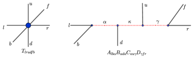
Figure 1: The representation of the initial tensor and its decomposition into triads for a three-dimensional system. The contracted indices are shown by red dashed lines.

III Results

III.1 $\mu=0$, $h=0$

In this subsection, we will discuss the $O(2)$ model without chemical potential or magnetic field. For $\mu=0$ and $h=0$ the initial local tensor (II) simplifies to

$$T_{lrudfb} =\sqrt{I_{l}(\beta)I_{r}(\beta)I_{u}(\beta)I_{d}(\beta)I_{f}(\beta)I_{b}(\beta)}\,\delta_{l+u+f}^{r+d+b}.$$ (9)

In this case, all the external triad legs carry the same weights. One of the observables we compute is the “internal energy”

$$E=-\frac{1}{V}\frac{\partial\ln Z}{\partial\beta}.$$ (10)

We show that the results obtained using the triad tensor method agree with those from the MC approach, as illustrated in Fig. 2.

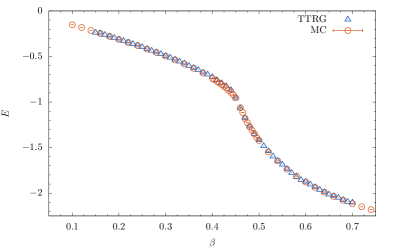
Figure 2: The internal energy obtained using triad TRG with $D=50$, and finite differences with $\Delta\beta=0.02$, agrees with the MC results on a lattice volume of $32^{3}$.

In order to determine the critical coupling, we compute the second $\beta$ derivative of the logarithm of the partition function to determine the “specific heat”,

$$C_{\rm v}=\frac{\beta^{2}}{V}\frac{\partial^{2}\ln Z}{\partial\beta^{2}}.$$ (11)

Our results shown in Fig. 3 clearly indicate that there is a peak in the specific heat corresponding to the second-order phase transition in this model. The location of the peak is consistent with high-precision results of earlier studies. The triad data are computed with $D=72$ using second-order finite differences with step size $\Delta\beta=0.01$. Decreasing the step size to reduce discretization errors is problematic as the systematic errors on $\ln Z$ cause large fluctuations on the standard finite-difference derivatives, and one would require a larger bond dimension ($D$) or more sophisticated numerical derivative computations to achieve a precise determination of the peak. The results of such an improvement for the original HOTRG method can be seen in Fig. 3 for $D=15$, where we get a smooth behavior for the specific heat, including the steep phase-transition region. These data were obtained using a stabilized second-order finite-difference scheme with step size reduced to $\Delta\beta=10^{-6}$. The stabilized finite-difference scheme was developed to avoid jumps between values of $\ln Z$ computed on close-by parameter values required for the evaluation of finite differences. Typically such jumps are caused by degenerate singular values or level crossings of singular values, leading to discontinuous changes of the vector subspaces used to truncate the coarse-graining tensors. The stabilization uses a heuristic approach that operates on the singular vectors of HOTRG to maximize the overlap between the adjacent vector subspaces (adjacent under a small change of $\beta$ in this case). These stabilized subspaces then improve the smoothness of $\ln Z$ for adjacent parameter values used to compute finite-difference derivatives. The application of stabilized finite differences to triads is more subtle and left for future work. Note that observables can also be computed using the impurity method (e.g., first order for the energy, second order for the specific heat). Although this method yields smoother data (which does not necessarily mean more accurate) than the finite difference method, it has an additional systematic error because the same matrices of singular vectors are used to truncate the pure and impure tensors.

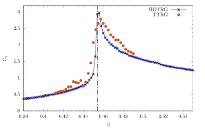
Figure 3: The specific heat capacity as a function of $\beta$ for a $32^{3}$ lattice volume. The triad data (orange) are computed with $D=72$ using a second-order finite difference of $\ln Z$ with step size $\Delta\beta=0.01$. The HOTRG data (blue) used $D=15$ and are computed with a stabilized second-order finite-difference scheme with $\Delta\beta=10^{-6}$. The peak of $C_{\rm v}$ suggests that the critical coupling is between $\beta=0.45$ and $\beta=0.46$. For reference, we show the infinite-volume MC result $\beta_{\rm{c}}=0.454165$ from Xu:2019mvy by the black dashed line.

III.2 $\mu=0$, $h\neq 0$

In this subsection, we study the model in the presence of a small symmetry-breaking external field $h$. The global $O(2)$ symmetry is broken and the partition function is given by

$$Z =\int d\Theta\prod_{i}e^{\beta h\cos\theta_{i}}\prod_{\nu=0}^{2}e^{\beta\cos(\theta_{i}-\theta_{i+\hat{\nu}})}.$$ (12)

One can compute the magnetization by either taking a numerical derivative of $\ln Z$ with respect to $h$ or by inserting an impurity tensor in the tensor network. Here we use the latter method with the impurity tensor given by

$$\widetilde{T}_{lrudfb} =\frac{1}{2}\sqrt{I_{l}(\beta)I_{r}(\beta)I_{u}(\beta)I_{d}(\beta)I_{f}(\beta)I_{b}(\beta)}$$

$$\times\Big{(}I_{l+u+f-r-d-b+1}(\beta h)+I_{l+u+f-r-d-b-1}(\beta h)\Big{)}.$$ (13)

From $\widetilde{T}_{lrudfb}$ and $T_{lrudfb}$ we can then compute the magnetization density as

$$M=\frac{1}{V}\sum_{i}\langle\cos\theta_{i}\rangle=\frac{1}{\beta V}\frac{\partial\ln Z}{\partial h}=\frac{\operatorname{tTr}(\widetilde{T}T^{V-1})}{\operatorname{tTr}(T^{V})}.$$ (14)

The results we obtained for the average magnetization density are shown in Fig. 4. For $\beta<\beta_{c}$, the spins are randomly distributed and average to zero, while for $\beta>\beta_{c}$ they prefer to align, resulting in a non-zero net magnetization. As we explore smaller $h$, we see that the change of behavior is consistent with the critical coupling obtained from the peak of the specific heat.

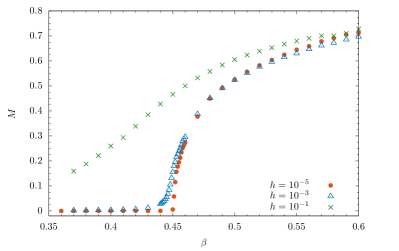
Figure 4: The magnetization of the $O(2)$ model for different external magnetic fields. We see that for sufficiently small symmetry-breaking field, the magnetization rises sharply around $\beta_{c}$. These results are obtained on a lattice of volume $(2^{13})^{3}$ with $D=30$.

III.3 $\mu\neq 0$, $h=0$

In this subsection, we consider the $O(2)$ model in the presence of a chemical potential, for which the action was already given in (1). This generalization is a problem for standard MC methods because the probability distribution in the partition function becomes complex and the sign problem is encountered (like for QCD at non-zero baryon density). Some numerical methods devised to circumvent the sign problem are reweighting, complex Langevin, thimbles, density of states, and dual variables. Reweighting enables the use of importance sampling MC, but only at an exponential cost, which makes it unusable for any practical purpose. The complex Langevin method uses a complexification of the spin degrees of freedom, however, measurements on the enhanced partition function are only equivalent to those on the original one if specific conditions concerning the probability distribution of the drift term in the complex plane are met Aarts:2011ax; Nagata:2016vkn. For the three-dimensional $O(2)$ model, the method does not satisfy these conditions in the disordered phase ($\beta\leq\beta_{c}$) and the method produces erroneous results Aarts:2010aq.

The method of choice to tackle the sign problem in the three-dimensional $O(2)$ model is to introduce dual variables, as discussed in Sec. II, and integrate out the original spin degrees of freedom. The ensuing partition function is free of a sign problem, even in the presence of a chemical potential. Once rewritten in this way the partition function can be simulated by the worm algorithm Prokof_ev_2001, as was done successfully in Banerjee:2010kc; Langfeld:2013kno.

Once reformulated in terms of dual variables, it turns out that the partition function can also be interpreted as a tensor network (6), and tensor-network methods can be applied in a straightforward way, as discussed in Sec. II. The only effect of the chemical potential is to modify the tensor entries depending on the value of their temporal indices,

$$T_{lrudfb} =\sqrt{I_{l}(\beta)I_{r}(\beta)I_{u}(\beta)I_{d}(\beta)I_{f}(\beta)I_{b}(\beta)e^{(u+d)\mu}}$$

$$\times\delta_{l+u+f}^{r+d+b}.$$ (15)

Note that even if a sign problem would remain after dualization, which would require reweighting in the worm algorithm, this would not be an issue for the tensor-network method which is deterministic in its construction and remains unaffected by such inconveniences, at least concerning the methodology.

One of the interesting observables at non-zero chemical potential is the particle number density (or charge density) defined as

$$\rho=\frac{1}{V}\frac{\partial\ln Z}{\partial\mu}.$$ (16)

In this subsection, we will investigate two important aspects of the $O(2)$ model at non-zero chemical potential: the Silver Blaze phenomenon at zero temperature and the temperature dependence of $\rho$, which is studied using asymmetric lattices.

As will be detailed below, we observe that for symmetric lattices the number density remains zero up to some threshold $\mu=\mu_{c}$ and then becomes non-zero, confirming the results of Ref. Langfeld:2013kno. This is a phenomenon occurring at strictly zero temperature since there the thermodynamic quantities are independent of $\mu$ when $\mu<\mu_{c}$, i.e., as long as $\mu$ is below the mass of the lightest excitation (or mass gap). In this case, no particle excitations can be generated and the particle number density is independent of $\mu$. This has been dubbed as the Silver Blaze phenomenon in studies of various lattice theories Cohen:2003kd.

The Silver Blaze phenomenon is especially hard to reproduce numerically as it is closely related to the cancellations in the original partition function which also lead to the sign problem. This is seen in MC simulations when reweighting from the phase quenched to the full theory. In the phase quenched theory the complex action is replaced by its real part, i.e., the weights in the original partition function are replaced by their magnitude. The phase quenched theory has no Silver Blaze, i.e., the particle number steadily increases with $\mu$. In this case, the Silver Blaze property of the full theory should emerge from large cancellations of the phase, however, only at an exponential cost Aarts:2013bla. Such reweighting simulations of the $O(2)$ model clearly show that the Silver Blaze is beyond reach using such methods.

However, as can be seen in Fig. 5, the Silver Blaze can be nicely reproduced, both by the worm algorithm and by the tensor method used in this work, and the results from both methods are in good agreement. In our tensor-network calculations, $\rho$ is computed using finite differences of $\ln Z$. We used a relatively small lattice size of $64^{3}$, which is primarily due to the large cost of the worm algorithm as the volume increases. For the range of $\beta$ values considered in the figure, this does not affect the results as the correlation lengths are small compared to the box size. This was also verified using tensor computations with volumes up to $1024^{3}$ which gave results similar to $64^{3}$. In Fig. 5, we show how the threshold $\mu_{c}$ varies with the coupling $\beta$ as we approach the continuum limit, i.e., $\beta\to\beta_{c}$ where the lattice spacing $a\to 0$. As expected, we see that in the bare theory the threshold tends to zero as $\beta\to\beta_{c}$. If we were to renormalize the lattice quantum field theory (see Langfeld:2013kno) and set the lattice spacing in physical units, the physical chemical potential $\mu_{\text{ph}}=\mu/a$, would have a threshold $(\mu_{c})_{\text{ph}}$ corresponding to the particle mass, independently of the value of $\beta$ in the vicinity of $\beta_{c}$ (up to discretization errors).

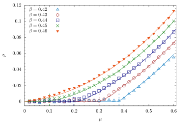
Figure 5: We compare the results obtained using triad TRG (symbols) with $D=50$ and worm algorithm (smooth lines) for the dependence of $\rho$ on $\mu$ for some values of the coupling $\beta$ on both sides (phases) of the critical coupling on a lattice of size $64^{3}$. We mark the threshold value $\mu_{c}$ which is related to the mass gap. It is clear that the mass gap decreases (and correlation length increases) as we go from $\beta=0.42$ to $\beta=0.45$ and would go to the CFT limit as $\beta\to\beta_{c}\approx 0.45417$.

We can also use the tensor methods to study the $O(2)$ model at non-zero temperature. For this we note that the extent of the Euclidean time axis is inversely proportional to the physical temperature, i.e., $T=1/(N_{t}a)$. The temperature can be set by varying the number of temporal sites $N_{t}$, and can be further fine-tuned by changing the coupling $\beta$ which determines the lattice spacing.

In standard HOTRG, the iterative coarse-graining procedure alternates between the different directions, here $t,x,y$, until the complete network has been reduced to a single tensor. This is a natural (although not necessarily best) coarse-graining order for an isotropic tensor on a symmetric lattice ($N_{t}=N_{x,y}$).

In the case of asymmetric lattices ($N_{t}\neq N_{x,y}$) a different strategy is often employed to compute results for varying values of $N_{t}$, i.e., temperatures, in an efficient way. The procedure consists of performing all spatial contractions on a single time slice to produce a time transfer matrix Zou:2014rha. This time transfer matrix is then multiplied to itself to attain the required number of time slices. Unfortunately, it turns out that such a procedure only converges to the correct result, obtained using the worm algorithm, for large $N_{t}$ (zero temperature) and often yields substantial deviations for non-zero temperatures. An alternative procedure is used in Ref. Kuramashi:2018mmi where finite temperature results are obtained in 2+1-dimensional $Z_{2}$ gauge theory for small $N_{t}$ by completely contracting the temporal direction first, and then coarse-graining the remaining spatial directions.

For anisotropic tensors, e.g., caused by a chemical potential, special care has to be taken to the coarse-graining order, i.e., the order in which the directions get contracted, to avoid large truncation errors. We therefore developed a method that implements an improved contraction order (ICO). This new method dynamically selects the next contraction direction to minimize the local truncation error. Its flexibility also makes it very useful for the treatment of asymmetric lattices and the method performs well for both small and large $N_{t}$. The ICO method was implemented as an enhancement of the standard HOTRG method. It was not yet implemented for the TTRG method because of the peculiar anisotropy of the triad factorization.

To validate the non-zero temperature tensor results we used the worm algorithm Prokof_ev_2001 at non-zero $\mu$ and find good agreement. This is illustrated in Fig. 6 where we show the temperature dependence of the 3d $O(2)$ model by studying the system on a $64^{2}\times N_{t}$ lattice for $N_{t}=2,4,8,16$. The tensor results were obtained using the ICO enhanced HOTRG method with $D=13$. The particle number density was computed using a stabilized finite-difference scheme (see Subsec. III.1), and tensor manipulations were performed using the TBLIS library matthews2016highperformance.

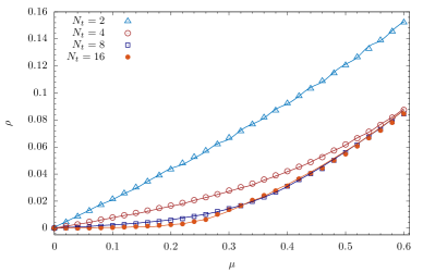
Figure 6: We use HOTRG with $D=13$, improved contraction order and stabilized finite differences to compute the particle density $\rho$ for a $64^{2}\times N_{t}$ lattice with $N_{t}=2,4,8,16$ (symbols) at $\beta=0.44$ and compare to the results obtained using worm algorithm (smooth lines). There is clear indication that as we move towards zero temperature, the behavior we see in Fig. 5 starts to emerge.

IV Summary and Discussion

In this work, we have carried out the first tensor-network study of the 3d classical $O(2)$ model at both zero and non-zero magnetic field, chemical potential, and temperature. The results obtained for the internal energy and the specific heat are consistent with MC data. However, our determination of the critical coupling is several orders of magnitude less precise than state-of-the-art MC results. We calculated the magnetization in the presence of a small magnetic field by inserting an impure tensor. At non-zero chemical potential, we were able to reproduce the Silver Blaze phenomenon at zero temperature. We considered non-zero temperature by varying the temporal extent of the lattice and computed the particle density at non-zero chemical potential. Our results agree with those obtained with the worm algorithm.

In the appendix, we discuss the convergence of $\ln Z/V$ with the bond dimension $D$. We expect that this convergence will play a key role in a more precise determination of $\beta_{c}$ and in exploring the corresponding field-theory limit in the future. To this end, improved coarse-graining schemes will have to be developed. Such improvements will also be useful to explore other interesting spin models in the future.

Appendix

It is a known problem that the truncations used in tensor-network methods sometimes lead to drastic modifications of the properties of the model whose thermodynamic behavior one intends to study. In this appendix, we investigate the convergence of $\ln Z/V$ with the local bond dimension $D$ in the triad approximation of HOTRG, in the large-volume limit for the three-dimensional cubic Ising and $O(2)$ models. We tune the couplings close to their critical values to make the dependence on $D$ prominent. This is illustrated in Figs. LABEL:fig:7 and LABEL:fig:8. The shaded areas enclose the various fits to the data (corresponding to various fit ranges and different fit formulas, including the Ansatz $a+bD^{-c}$). The extrapolation to $D\to\infty$ can be read off from the intercept with the vertical axis. The convergence for the Ising model is faster than for the $O(2)$ model, which may hint to a different efficiency of tensor methods for systems with discrete and continuous symmetries. In order to explore the field-theory limit and for the determination of the critical exponents, the infinite-$D$ value of $\ln Z/V$ is required to good accuracy. It seems that the current tensor computations are still somewhat far away from that desired limit. An advance in constructing better algorithms that converge faster without increasing time or memory complexity would be desirable in the future.

The numerical computations were mostly performed on a 2.4 GHz machine with about 180 GB of memory on a single core using the highly optimized opt_einsum Python module for tensor contractions Smith:2018aaa. We explored a maximum of $D=82$ for the $O(2)$ model which took about 62 hours for a lattice of volume $(2^{15})^{3}$ and about 18 hours for a lattice volume $(2^{5})^{3}$. We found that the computation time for the triad method scaled as $D^{6}$ within errors, even though our implementation of the algorithm asymptotically scales as $D^{7}$.