Deflation algorithm for the Green function of quasi-1D lattices

Abstract

We derive a method to efficiently compute the Green function of on arbitrary Hamiltonians defined on semi-infinite and periodic quasi-one-dimensional lattices. Computing the Green function is the backbone of quantum transport, electronic structure or linear response computations. Our method constitutes a “deflation optimization” of a well established algorithm often used in quantum transport that is based on generalized Schur factorizations of the linearized quadratic eigenvalue equation for the transfer matrix. Our deflation optimization may greatly reduce the number of degrees of freedom that must be processed in the Schur factorization. Deflation must be supplemented by a Jordan-block reconstruction of generalized eigenvectors, also developed here in detail. The overhead of deflation plus reconstruction is minimal as compared to the typical reduction in factorization runtime. Furthermore, by avoiding inverses of ill-conditioned matrices, the algorithm remains numerically stable.

A basic pillar of computational condensed matter physics is the retarded Green function of electrons Economou:83; Abrikosov:75; Haug:08. This quantity, denoted here as $G^{r}(t^{\prime}-t)$ (in the time domain) or $G^{r}(\omega)$ (in the frequency domain), represents the causal propagation in a given time interval $t^{\prime}-t$ of quantum particles or waves between two points in a stationary system. For numerical purposes, the system is often modeled using a tight-binding-like Hamiltonian on a lattice (constructed either ab-initio or phenomenologically). The non-equilibrium transport properties of the system without interactions or its spectral density, to name just two important examples, can be expressed fully in terms of $G^{r}$. The powerful Keldysh Green function formalism allows to cleanly extend non-interacting results to systems with interactions, in or out of equilibriumKeldysh:SPJ65; Kadanoff:62; Abrikosov:75; Rammer:RMP86; Meir:PRL92; Stefanucci:13. Accurate and performant methods to compute $G^{r}$ are a critical part in all these techniques.

When computing the retarded Green function directly in the frequency domain $G^{r}(\omega)$ (the form most relevant to steady-state transport or spectral density simulations – see e.g. Refs. Gaury:PR14; Weston:PRB16 for alternative real-time approaches), numerical methods can be broadly classified into two groups: full-band and single-shot. In the first group one obtains $G^{r}(\omega)$ at all values of $\omega$ simultaneously. Prominent examples are the Tetrahedron Method Rath:PRB75; MacDonald:JPCSSP79; Molenaar:JPC82; Blochl:PRB94; Zaharioudakis:CPC05; Kawamura:PRB14, that computes the non-interacting $G^{r}(\omega)$ from a sampling of the bandstructure of a periodic system, or the Kernel Polynomial MethodWeisse:RMP06; Joao:RSOS20; Fan:PR21, that uses Chebyshev expansion of functions of the system Hamiltonian, also without interactions. In both a price is paid in accuracy that can be reduced by increasing the sampling precision of the bandstructure or increasing the order of the expansion, respectively. In contrast, single-shot approaches Sanvito:PRB99; Rungger:PRB08 can typically compute $G^{r}(\omega)$ exactly (i.e. within machine precision), possibly in the presence of many-body self-energy corrections, at the expense of requiring one independent computation per frequency $\omega$. These are usually the preferred methods in normal transport and low-energy electronic structure simulations, wherein only electrons close to the Fermi energy are relevant. Of particular interest for mesoscopic transport are single-shot algorithms for periodic, quasi-one-dimensional (quasi-1D) systems, that allow to integrate out the semi-infinite quasi-1D leads connecting the system to electronic reservoirs Datta:97; Wimmer:09.

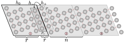
Figure 1: Sketch of a generic periodic quasi-1D lattice. Each shaded circle represents an orbital, with red lines representing arbitrary hoppings. There are $n$ orbitals in each unit cell. $h_{0}$ is the $n\times n$ intracell Hamiltonian matrix. An $r$-dimensional orbital subspace $P_{+}$ in each unit cell (dark gray box) is coupled through $h_{+}$ to the neighboring unit cell on the right (intercell hoppings), while $h_{-}$, typically the adjoint of $h_{+}$, couples a subspace $P_{-}$ (dashed box) to the neighboring unit cell on the left. The self-energy in the first unit cell $\Sigma^{r}_{11}$ is concentrated on $P_{+}$. When computing the Green function between any two orbitals in the lattice, the deflation technique effectively eliminates the $\bar{r}$-dimensional subspace orthogonal to $P_{+}$ from the problem.

In this paper we present a “deflation” technique that can substantially speed up the performance of one of the most common single-shot method for periodic quasi-1D systems, dubbed here the Schur methodWimmer:09, that is used in several numerical libraries for quantum transportGroth:NJOP14; Quantica:Z21. The core of this method is a generalized Schur factorization (also known as QZ decomposition) of a linearized version of the Dyson equation for the transfer matrix. We show that in many cases of interest a potentially large subspace of electronic orbitals can be eliminated (“deflated”) before the main Schur factorization step, which then becomes substantially faster due to its $O(n^{3})$ complexity in the number $n$ of orbitals in the lead unit cell. The deflation pre-processing needs to be supplemented with a generalized eigenvector computation in a post-processing step that reconstructs any generalized eigenvectors that are lost to deflation. The overhead added by the pre-processing and post-processing steps are found to be typically negligible as compared to the runtime gains in the central Schur step.

I The Schur method

Before developing the deflation and generalized eigenvector algorithms, we will first summarize the basic Schur method as developed in Ref. Wimmer:09. The Schur method solves, at each fixed $\omega$, the self-consistent Dyson equation $G^{r}(\omega)=g_{0}(\omega)+g_{0}(\omega)\Sigma^{r}(\omega)G^{r}(\omega)$ of a semi-infinite periodic lattice (a lead in transport simulations, see Fig. 1). Here $g_{0}(\omega)=(\omega+i\eta-h_{0})^{-1}$ is the $n\times n$ Green function matrix of an isolated, $n$-orbital lead unit cell, of Hamiltonian $h_{0}$, and $\Sigma^{r}(\omega)$ is the self-energy due to the coupling $h_{+}$ ($h_{-}$) of each unit cell to its right (left) neighboring cells. If we project the Dyson equation onto the first (leftmost) unit cell of the semi-infinite lead, we have $G^{r}_{11}=g^{r}_{0}+g^{r}_{0}\Sigma^{r}_{11}G^{r}_{11}$ (we omit the $\omega$ dependences for brevity), or equivalently

$$(g_{0}^{-1}-h_{-}G^{r}_{11}h_{+})G^{r}_{11}=1$$ (1)

where $\Sigma^{r}_{11}=h_{-}G^{r}_{11}h_{+}$ is the self-energy induced on the first unit cell by the remaining unit cells, and $G^{r}_{11}$ denotes the retarded Green function matrix between any two sites in the first unit cell. We rewrite this equation by multiplying with $h_{+}$ on the right and by defining the retarded transfer matrix $T^{r}=G^{r}_{11}h_{+}$,

$$h_{+}-g_{0}^{-1}T^{r}+h_{-}(T^{r})^{2}=0$$ (2)

If we assume $T^{r}$ is diagonalizable (which is not the case in general, as will be discussed below), we can write

$$T^{r}=G^{r}_{11}h_{+}=\Phi^{r}\Lambda^{r}\left(\Phi^{r}\right)^{-1},$$ (3)

where $\Phi^{r}$ is an $n\times n$ invertible matrix with the proper eigenvectors $\phi_{i}$ of $T^{r}$ as columns, and $\Lambda^{r}$ is a diagonal matrix with eigenvalues $\lambda_{i}$ in the diagonal, so that $T^{r}\phi_{i}=\lambda_{i}\phi_{i}$ for each eigenpair $\phi_{i}$, $\lambda_{i}$. By combining Eqs. (2) and (3), we see that all eigenpairs $\phi,\lambda$ satisfy a quadratic eigenvalue equation

$$(h_{+}-g_{0}^{-1}\lambda+h_{-}\lambda^{2})\phi=0$$ (4)

The transfer matrix also needs to satisfy retarded boundary conditions, which corresponds to a finite $\lim_{m\to\infty}(T^{r})^{m}$. This restricts the allowed (complex) eigenvalues $\lambda$ to lie on the unit circle or inside, $|\lambda|\leq 1$. If we rewrite $\lambda=e^{ika_{0}}$, where $a_{0}$ is the lead lattice period and $k$ is a real or complex wavevector, we may interpret Eq. (4) above as the Bloch equation for propagating ($|\lambda|=1$), right-evanescent ($|\lambda|<1$) or left-evanescent ($|\lambda|>1$) solutions at energy $\omega$ on an infinite version (instead of semi-infinite) of the lead lattice. To preserve causality we must restrict $\Phi^{r}$ to solutions with $|\lambda|\leq 1$, and among propagating ones ($|\lambda|=1$) keep only those with positive group velocity. These can be shown Wimmer:09 to become evanescent when $\omega$ acquires a small and positive imaginary part $i\eta$, as in the definition of $g_{0}(\omega)$. In practice, then, we define $\Phi^{r}$ simply as the set of eigenvectors with $|\lambda|<1$ when $\eta\to 0^{+}$. Assuming we can find $n$ such linearly independent retarded solutions (this is possible when $T^{r}$ is diagonalizable), $\Phi^{r}$ will be a full-rank, invertible matrix, which allows to build $T^{r}$ using Eq. (3) and solves the problem of finding $G^{r}_{11}$ through Eq. (1),

$$G^{r}_{11} = (g_{0}^{-1}-\Sigma^{r}_{11})^{-1}$$ (5)

$$\Sigma^{r}_{11} = h_{-}T^{r}=h_{-}\Phi^{r}\Lambda^{r}\left(\Phi^{r}\right)^{-1}$$

With $G^{r}_{11}$ we can also reconstruct $G^{r}_{NM}$ between any two unit cells $N$ and $M$, as explained in Appendix LABEL:ap:GNM.

The problem then reduces to finding all retarded solutions of Eq. (4). A powerful and quite common approach is to linearize the $n\times n$ quadratic eigenvalue problem into a $2n\times 2n$ generalized but linear eigenvalue problem $A\psi=\lambda B\psi$. This is done using one of several possible linearization transformations. The so-called first-companion linearization is probably simplest, and takes the following form

$$\Bigg{[}\overbrace{\left(\begin{array}[]{cc}0&1\\ -h_{+}&g_{0}^{-1}\end{array}\right)}^{A}-\lambda\overbrace{\left(\begin{array}[]{cc}1&0\\ 0&h_{-}\end{array}\right)}^{B}\Bigg{]}\overbrace{\left(\begin{array}[]{c}\phi\\ \chi\end{array}\right)}^{\psi}=(A-\lambda B)\psi=0$$ (6)

Each advanced $|\lambda|>1$ or retarded $|\lambda|<1$ solution to the above corresponds to one and only one solution of the original quadratic eigenvalue problem, where $\chi=\lambda\phi$. At a low level, numerical libraries such as LAPACK Anderson:99 compute the eigenpairs $\lambda,\psi$ in two steps. First, a generalized Schur (or QZ) factorization of $A,B$,

$$A-\lambda B=Q(S_{A}-\lambda S_{B})Z^{{\dagger}},$$ (7)

does the heavy lifting of finding unitary $2n\times 2n$ matrices $Q$ and $Z$ that transform $A$ and $B$ into upper triangular matrices $S_{A}$ and $S_{B}$, respectively. The diagonals $\alpha_{i}$ and $\beta_{i}$ of $S_{A}$ and $S_{B}$ can be shown to yield the eigenvalues $\lambda_{i}=\alpha_{i}/\beta_{i}$. The Schur factorization is numerically stable, and once obtained, efficient routines exist that can transform it into an equivalent Schur form with reordered diagonals of $S_{A},S_{B}$, wherein retarded eigenvalues ($|\alpha_{i}|<|\beta_{i}|$) appear before advanced eigenvalues. Then, a backsubstitution stage is used for each $\lambda$ to find the $\psi$ eigenvectors one by one. The resulting retarded and advanced eigenvectors $\psi$ can be written as the columns of the matrix $\Psi=ZR$, where $R$ is the backsubstitution upper-triangular matrix. If the factorization was reordered with retarded solutions coming first, we have

$$\Psi=\left(\begin{array}[]{cc}\Phi^{r}&\Phi^{a}\\ \Phi^{r}\Lambda^{r}&\Phi^{a}\Lambda^{a}\end{array}\right)=\left(\begin{array}[]{cc}Z_{11}&Z_{12}\\ Z_{21}&Z_{22}\end{array}\right)\left(\begin{array}[]{cc}R_{11}&R_{12}\\ 0&R_{22}\end{array}\right),$$ (14)

where we have also included the advanced $\Phi^{a}$, $\Phi^{a}\Lambda^{a}$ blocks with $|\lambda|>1$. Note that $\Phi^{r}=Z_{11}R_{11}$ and $\Phi^{r}\Lambda^{r}=Z_{21}R_{11}$. This expression allows us to interpret $Z_{11}$ as the basis of the invariant subspaces spanned by subsets of eigenstates $\Phi^{r}$, and $R_{11}$ as the eigenstate coordinates in this basis. (Similarly for $Z_{21}$ and states $\Phi^{r}\Lambda^{r}$.) Crucially, the $T^{r}$ matrix is independent of the coordinate matrix $R$, since

$$T^{r}=\Phi^{r}\Lambda^{r}\left(\Phi^{r}\right)^{-1}=Z_{21}R_{11}R_{11}^{-1}Z_{11}^{-1}=Z_{21}Z_{11}^{-1}$$ (15)

This is a very significant advantage of the Schur method, and a common theme throughout this work. We can construct $T^{r}$ matrix, and hence the Green function, without needing to actually compute matrix $R$ or eigenstates $\Phi^{r}$. Only the bases $Z_{11}$ and $Z_{21}$ of the invariant subspaces is needed. This is an important advantage numerically, since it also bypasses the need to invert $\Phi^{r}$, which can be numerically unstable (note that since $T^{r}$ is non-Hermitian, so its eigenstates can be almost parallel and even coalesce, yielding ill-conditioned or even singular $R_{11}$). In contrast to $R_{11}^{-1}$, the inverse $Z_{11}^{-1}$ is typically found to be well conditioned, since it is an $n\times n$ block of the $Z$ unitary matrix. A further, often overlooked advantage is that Eq. 15 gives the correct retarded solution of Eq. (2) even if the resulting $T^{r}$ is defective (non-diagonalizable), i.e. when $T^{r}$ has only $r<n$ linearly independent proper eigenvectors, making $R$ strictly rank-deficient and thus non-invertible.

II The deflation technique

The main practical drawback of the Schur method as presented here is the fact that its theoretical computational complexity grows with the cube of the number of orbitals $n$, which can prove to be a challenge for large unit cells. The deflation technique presented in this section optimizes the Schur factorization step by removing all $\lambda=\infty$ advanced eigenvectors and all $\lambda=0$ retarded eigenvectors from the problem. Note that neither of these contribute to $T^{r}$ as given in Eq. (3). The existence of retarded $\lambda=0$ ($\lambda=\infty$) eigenvectors is a consequence matrix $h_{+}$ ($h_{-}$) having a non-empty kernel in general. Indeed, if a non-zero vector $\phi_{0}$ belongs to $\mathrm{ker}(h_{+})$ it will be a $\lambda=0$ eigenvector, since by definition $T^{r}\phi_{0}=G^{r}_{11}h_{+}\phi_{0}=0$. Geometrically, any orbitals in an $n$-orbital unit cell not directly coupled by $h_{+}$ to the neighboring unit cell on the right will belong to $\mathrm{ker}(h_{+})$, see Fig. 1. By removing all $\bar{r}=n-r=\mathrm{dim}\,\mathrm{ker}(h_{+})$ solutions with $\lambda=0$ beforehand, we may transform the $2n\times 2n$ Schur factorization step of Eq. (7) into a $2r\times 2r$ factorization, roughly yielding a $\sim(r/n)^{3}$ reduction in runtime. The deflation technique is a prescription for building a smaller $2r\times 2r$ linear pencil $A_{2}-\lambda B_{2}$ which however shares the same spectrum as pencil $A-\lambda B$ in Eq. (6) except for any $\lambda=0$ and $\lambda=\infty$ solutions. The only requirement for the deflation technique in this section to work is that $\mathrm{ker}(h_{+})=\mathrm{ker}(h_{-}^{{\dagger}})$, which is guaranteed for Hermitian lattice Hamiltonians with $h_{+}=h_{-}^{{\dagger}}$. In Appendix LABEL:ap:quadeig we sketch a more elaborate deflation procedure (a variation of the so-called quadeig algorithm Hammarling:ATMS13; Drmac:19) that works also with arbitrary $h_{\pm}$. Throughout this section we also assume that $T^{r}$ is non-defective. The fully general algorithm for the defective case will be completed in Sec. LABEL:sec:defective.

The first step is to find orthonormal bases $\bar{P}_{+}$ and $P_{+}$ of $\mathrm{ker}(h_{+})$ and its orthogonal complement, respectively. The $\bar{P}_{+}$ matrix is $\bar{r}\times n$ , and $P_{+}$ is $r\times n$, with $r+\bar{r}=n$, so that together they form a unitary $n\times n$ matrix $Q_{+}=(P_{+}\bar{P}_{+})$. It can be efficiently computed using a pivoted LQ decomposition of $h_{+}$,

$$h_{+}=\pNiceMatrix[first-row,code-for-first-row=\scriptstyle,code-for-last-col=\scriptstyle]r&\bar{r}\\ L_{+}0\pNiceMatrix[first-row,code-for-first-row=\scriptstyle,code-for-last-col=\scriptstyle]n\\ P_{+}^{{\dagger}}\\ \bar{P}_{+}^{{\dagger}}=\pNiceMatrix L&0Q_{+}^{{\dagger}},$$ (16)

so that

(17)

(18)

(19)

(20)

(21)

(22)

ThefirstcompanionlinearizationinEq.(

6)istransformedundertheunitarytransformation

$$Q_{1}=\pNiceMatrix Q$$

&0 0Q+intoA1-λB1=Q1†(A-λB)Q1,andtheexpandedeigenvectorsintoψ1=Q1†ψ=(ϕr,ϕ¯r,χr,χ¯r)T,whereϕr=P†+ϕrepresentstheprojectionoftheeigenstateontheright`surface′oftheunitcell,andϕ¯r=¯P†+ϕitsorthogonal.Theeigenvalueequation(A1-λB1)ψ1=0thenreads

$$\Bigg{[}\overbrace{\pNiceMatrix 0&010{\\ }0001{\\ }-V_{+}0g_{0rr}^{-1}g_{0r\bar{r}}^{-1}{\\ }-\bar{V}_{+}0g_{0\bar{r}r}^{-1}g_{0\bar{r}\bar{r}}^{-1}}^{A_{1}}-\lambda\overbrace{\pNiceMatrix 1&000{\\ }0100{\\ }00V_{-}\bar{V}_{-}{\\ }0000}^{B_{1}}\Bigg{]}\overbrace{\pNiceMatrix\phi_{r}{\\ }\phi_{\bar{r}}{\\ }\chi_{r}{\\ }\chi_{\bar{r}}}^{\psi_{1}}=0$$ (23)

Inthisbasisweimmediatelyseethatonlytheϕr,χrandχ¯reigenvectorcomponentsarecoupled,withϕ¯rdecouplingaway,andgivensimplybyϕ¯r=λ-1χ¯ronceχ¯risknown(unlessλ=0).Wearethusleftwith

$$\Bigg{[}\overbrace{\pNiceMatrix 0&10{\\ }-V_{+}g_{0rr}^{-1}g_{0r\bar{r}}^{-1}{\\ }-\bar{V}_{+}g_{0\bar{r}r}^{-1}g_{0\bar{r}\bar{r}}^{-1}}^{\tilde{A}_{1}}-\lambda\overbrace{\pNiceMatrix 1&00{\\ }0V_{-}\bar{V}_{-}{\\ }000}^{\tilde{B}_{1}}\Bigg{]}\overbrace{\pNiceMatrix\phi_{r}{\\ }\chi_{r}{\\ }\chi_{\bar{r}}}^{\tilde{\psi}_{1}}=0$$ (24)

Bycastingtheeigenprobleminthisformwehaveimplicitlydroppedallλ=0solutions,whichhaveafiniteϕ¯rwithallothercomponentsequaltozero.Fromthelastblock-rowwenowseethatany~ψ1=(ϕr,χr,χ¯r)Teigenvectorwithλ≠∞mustbelongtothekernelofC2=-¯V+&g0¯rr-1g0¯r¯r-1.C2isamatrixofsize¯r×(n+r)=(n-r)×(n+r),soitkernelisatleastofdimension2r.Wecomputeanorthonormalbasis¯P2ofker(C2)throughanotherLQfactorization

$$C_{2}=\pNiceMatrix-\bar{V}$$ (25)

&g0¯rr-1g0¯r¯r-1=[first-row,code-for-first-row=]¯r&2r L20[first-row,code-for-first-row=]n+r P2† ¯P†2Wedefineψ2=¯P†2~ψ1asthe2rcomponentsof~ψ1