Perfectly-matched-layer truncation is exponentially accurate at high frequency

Abstract.

We consider a wide variety of Helmholtz scattering problems including scattering by Dirichlet, Neumann, and penetrable obstacles. We consider a radial perfectly-matched layer (PML) and show that for any fixed PML width and a steep-enough scaling angle, the PML solution is exponentially close, both in frequency and the tangent of the scaling angle, to the true scattering solution. Moreover, for a fixed scaling angle and large enough PML width, the PML solution is exponentially close to the true scattering solution in both frequency and the PML width. In fact, the exponential bound holds with rate of decay $c(w\tan\theta-C)k$ where $w$ is the PML width and $\theta$ is the scaling angle. More generally, the results of the paper hold in the framework of black-box scattering under the assumption of an exponential bound on the norm of the cutoff resolvent, thus including problems with strong trapping. These are the first results on the exponential accuracy of PML at high-frequency with non-trivial scatterers.

1. Introduction

1.1. Context and background

Since the work of Berenger [Ber94], perfectly matched layers (PMLs) have become a standard tool in the numerical simulation of frequency-domain wave problems such as the Helmholtz equation. This method approximates the solution of a scattering problem in an unbounded domain by making a complex change of variables in a layer away from the region of interest and truncating the problem with a Dirichlet condition.

It is well known that, for fixed frequency, the error in the truncation decreases exponentially with the width of the perfectly matched layer (PML); see [LS98, Theorem 2.1], [LS01, Theorem A], [HSZ03, Theorem 5.8], [BP07, Theorem 3.4]. However these error bounds are not explicit in the frequency.

The only frequency-explicit error bounds on the accuracy of PMLs obtained up till now are for the model problem of no scatterer. In this case, the error is known to decrease exponentially in the width of the PML, the tangent of the scaling angle, and the frequency; this was proved in [CX13, Lemma 3.4] (for $d=2$) and [LW19, Theorem 3.7] (for $d=2,3$) using the fact that the solution of this problem can be written explicitly.

In this paper, we consider a wide variety of Helmholtz scattering problems, including scattering by Dirichlet, Neumann, and penetrable obstacles in any dimension, and including problems with strong trapping. We consider a radial PML and prove that, provided that the PML change of variables is $C^{3}$, the error decreases exponentially in frequency, the PML width, and the scaling angle with a rate that, at least in one dimension, is sharp.

We first state these results applied to the particular problem of plane-wave scattering by an impenetrable obstacle in §1.2, and then state the results in the “black-box scattering” framework in §1.3.

1.2. The main results applied to plane-wave scattering by an impenetrable obstacle

Let $\Omega_{-}\subset\mathbb{R}^{d}$ be bounded and open with Lipschitz boundary $\Gamma_{-}:=\partial\Omega_{-}$ and connected open complement, $\Omega_{+}:=\mathbb{R}^{d}\setminus\Omega_{-}$. Truncation by a PML is widely used to compute approximations to the exterior Helmholtz problem

(1.1) $$\begin{gathered}(-\Delta-k^{2})u^{S}=0\text{ in }\Omega_{+},\qquad Bu^{S}=-B\exp(ikx\cdot a)\text{ for }x\in\Gamma_{-},\\ (\partial_{r}-ik)u^{S}=o(r^{\frac{1-d}{2}})\text{ as }r:=|x|\to\infty.\end{gathered}$$

Here, $B$ is an operator on the boundary giving either the Dirichlet (sound-soft) condition, $u\mapsto u|_{\Gamma_{-}}$ or Neumann (sound-hard) condition $u\mapsto(\partial_{\nu}u)|_{\Gamma_{-}}$, and $\nu(x)$ is the outward unit normal to $\Omega_{-}$. Physically, $u^{S}$ corresponds to the scattered wave generated when the plane wave $\exp(ikx\cdot a)$ hits the obstacle $\Omega_{-}$.

Let $R_{P}(k)$ denote the solution operator for (1.1) (see Proposition 2.1 for the precise definition); the letter $R$ stands for “resolvent”, and the subscript $P$ is there because we use this notation for the solution operator for the more-general operator $P$ in §1.3 below. Let $\chi\in C_{c}^{\infty}(\mathbb{R}^{d})$ with $\chi\equiv 1$ in a neighbourhood of the convex hull of $\Omega_{-}$. We define the exponential rate of growth for the solution operator through a subset $J\subset\mathbb{R}$ that is unbounded above:

(1.2) $$\Lambda(P,J):=\limsup_{\begin{subarray}{c}k\to\infty\\ k\in J\end{subarray}}\frac{1}{k}\log\|\chi R_{P}(k)\chi\|_{L^{2}\to L^{2}}.$$

We write $\Lambda(P)$ for $\Lambda(P,\mathbb{R})$. If $\Gamma_{-}$ is $C^{\infty}$ then $\Lambda(P)<\infty$. If, in addition, $\Gamma_{-}$ is nontrapping, then $\Lambda(P)=0$. Finally, if $\Gamma_{-}$ is only Lipschitz, then for all $\delta>0$ there is a set $J\subset\mathbb{R}$ with $|\mathbb{R}\setminus J|\leq\delta$ such that $\Lambda(P,J)=0$; see §1.3 and §2.1 for details and references.

Figure 1.1. The diagram shows the obstacle, $\Omega_{-}$, the ball of radius $R_{1}$ (outside of which the scaling begins), the ball of radius $R_{{\rm tr}}$, and $\Omega_{{\rm tr},+}$ (shaded in the hatched lines) where the domain exterior to $\Omega_{-}$ is truncated.

We now describe the geometric set-up for the PML truncation; see Figure 1.1 for a schematic. Let $R_{2}>R_{1}>0$, such that $\Omega_{-}\Subset B(0,R_{1})$. Next, let $R_{{\rm tr}}>R_{1}$ and $\Omega_{{\rm tr}}\subset\mathbb{R}^{d}$ be a bounded Lipschitz open subset with $B(0,R_{{\rm tr}})\subset\Omega_{{\rm tr}}$. Finally, let $\Omega_{{\rm tr},+}:=\Omega_{{\rm tr}}\cap\Omega_{+}$, $\Gamma_{{\rm tr}}:=\partial\Omega_{{\rm tr}}$, and $0\leq\theta<\pi/2$. The PML method replaces (1.1) by the following problem

(1.3) $$(-\Delta_{\theta}-k^{2})v^{S}=0\text{ in }\Omega_{{\rm tr},+},\qquad Bv^{S}=-B\exp(ikx\cdot a)\text{ for }x\in\Gamma_{-},\qquad v^{S}=0\text{ for }x\in\Gamma_{{\rm tr}}.$$

Here, $-\Delta_{\theta}$ is a second order differential operator that is given in spherical coordinates $(r,\omega)\in[0,\infty)\times S^{d-1}$ by

(1.4) $$\Delta_{\theta} =\Big{(}\frac{1}{1+if_{\theta}^{\prime}(r)}\partial_{r}\Big{)}^{2}+\frac{d-1}{(r+if_{\theta}(r))(1+if^{\prime}_{\theta}(r))}\partial_{r}+\frac{1}{(r+if_{\theta}(r))^{2}}\Delta_{\omega},$$

$$=\frac{1}{(1+if_{\theta}^{\prime}(r))(r+if_{\theta}(r))^{d-1}}\frac{\partial}{\partial r}\left(\frac{(r+if_{\theta}(r))^{d-1}}{1+if_{\theta}^{\prime}(r)}\frac{\partial}{\partial r}\right)+\frac{1}{(r+if_{\theta}(r))^{2}}\Delta_{\omega},$$

with $\Delta_{\omega}$ the surface Laplacian on $S^{d-1}$ and $f_{\theta}(r)\in C^{3}([0,\infty);\mathbb{R})$ given by $f_{\theta}(r)=f(r)\tan\theta$ for some $f$ satisfying

(1.5) $$\begin{gathered}\{f(r)=0\}=\{f^{\prime}(r)=0\}=\{r\leq R_{1}\},\qquad f^{\prime}(r)\geq 0,\qquad f(r)\equiv r\text{ on }r\geq R_{2};\end{gathered}$$

i.e., the scaling “turns on” at $r=R_{1}$, and is linear when $r\geq R_{2}$. We emphasize that $R_{{\rm tr}}$ can be $<R_{2}$, i.e., we allow truncation before linear scaling is reached. Indeed, $R_{2}>R_{1}$ can be arbitrarily large and therefore, given any bounded interval $[0,R]$ and any function $g\in C^{3}([0,R])$ satisfying

(1.6) $$\begin{gathered}\{g(r)=0\}=\{g^{\prime}(r)=0\}=\{r\leq R_{1}\},\qquad g^{\prime}(r)\geq 0,\end{gathered}$$

our results hold for an $f$ with $f|_{[0,R]}=g$. A concrete example of a $g(r)$ satisfying the conditions (1.6) is the piecewise degree-three polynomial

(1.7) $$g(r)=(r-R_{1})^{3}1_{[R_{1},\infty)}(r).$$

Remark 1.1 (Link with notation used in the numerical-analysis literature).

In (1.3)-(1.5) the PML problem is written using notation from the method of complex scaling (see, e.g., [DZ19, §4.5]). In the numerical-analysis literature on PML, the scaled variable is often written as $r(1+i\widetilde{\sigma}(r))$ with $\widetilde{\sigma}(r)=\sigma_{0}$ for $r$ sufficiently large, see, e.g., [HSZ03, §4], [BP07, §2]. To convert from our notation, set $\widetilde{\sigma}(r)=f_{\theta}(r)/r$ and $\sigma_{0}=\tan\theta$. We also highlight that, whereas the numerical-analysis literature on radial PMLs often assumes that the exterior domain is truncated by a ball (i.e., $\Omega_{{\rm tr}}=B(0,R_{PML})$ for some $R_{PML}>R_{1}$), the PML problem (1.3) is posed with a general truncation boundary. One practical advantage of allowing an arbitrary truncation boundary is that, when solving the PML problem with the finite-element method (FEM) one can then use simplicial elements without having to deal with error in approximating the truncation boundary.

Theorem 1.2.

Let $\Gamma_{-}$ be Lipschitz and $J\subset\mathbb{R}$ unbounded above with $\Lambda(P,J)<\infty$. For all $\eta,\epsilon>0$ there exist $C,C^{\prime},k_{0},c_{\epsilon}>0$ (independent of $R_{{\rm tr}}$ and $R_{1}$) such that for all $R_{{\rm tr}}>R_{1}+\epsilon$, $B(0,R_{{\rm tr}})\subset\Omega_{{\rm tr}}\Subset\mathbb{R}^{d}$ with Lipschitz boundary, there exists $\theta_{0}(P,J,R_{{\rm tr}})<\pi/2$ (with $\theta_{0}(P,J,R_{{\rm tr}})$ a non-increasing function of $R_{\rm tr}$) such that if $\theta_{0}(P,J,R_{{\rm tr}})+\epsilon<\theta<\pi/2-\epsilon$, $k>k_{0}$ with $k\in J$, and $a\in\mathbb{R}^{d}$, then the solution $v^{S}$ to (1.3) exists, is unique, and satisfies

(1.8) $$\begin{gathered}\frac{\|u^{S}-v^{S}\|_{H^{1}(B(0,R_{1})\setminus\Omega_{-})}}{\|u^{S}+e^{ikx\cdot a}\|_{L^{2}(B(0,R_{1})\setminus\Omega_{-})}}\leq C\exp\Big{(}-k\big{(}(2-\eta)c_{\epsilon}(R_{{\rm tr}}-R_{1}-\epsilon)\tan\theta-2\Lambda(P,J)\big{)}\Big{)},\\ \|u^{S}-v^{S}\|_{H^{1}(B(0,R_{1})\setminus\Omega_{-})}\leq C^{\prime}\frac{\|u^{S}-v^{S}\|_{H^{1}(B(0,R_{1})\setminus\Omega_{-})}}{\|u^{S}+e^{ikx\cdot a}\|_{L^{2}(B(0,R_{1})\setminus\Omega_{-})}},\end{gathered}$$

where $u^{S}$ is the solution to (1.1). Furthermore, if $\Lambda(P,J)=0$, then $\theta_{0}(P,J,R_{{\rm tr}})=0$.

Theorem 1.2 shows that both the absolute and the relative error in the PML approximation of the total field $u^{S}+e^{ikx\cdot a}$ is exponentially small in $k$, the PML width (i.e., $R_{{\rm tr}}-R_{1}$), and the tangent of the scaling angle (i.e., $\tan\theta$).

Theorem 1.2 is a consequence of the following more general result, which gives explicitly the rate of decay and $\theta_{0}(P,J,R_{{\rm tr}})$. This result involves the following two functions;

(1.9) $$\Phi_{\theta}(r):=\begin{cases}\inf_{t\geq 0}\Big{|}\operatorname{Im}\Big{(}(1+if_{\theta}^{\prime}(r))\sqrt{1-\frac{t}{(r+if_{\theta}(r))^{2}}}\,\Big{)}\Big{|},&d\geq 2,\\ f_{\theta}^{\prime}(r),&d=1,\end{cases}$$

(1.10) $$\theta_{0}(P,J,R_{{\rm tr}}):=\sup\Big{\{}\theta\,:\,\int_{R_{1}}^{R_{{\rm tr}}}\Phi_{\theta}(r)\,dr\leq\Lambda(P,J)\Big{\}}.$$

To better understand these functions, we record the following:

• $\Phi_{\theta}(r)\geq 0$ for all $r$ (by definition), and $\Phi_{\theta}(r)>0$ when $r>R_{1}$ and $\theta>0$ (by Part (1) of Lemma 1.4 below).

• If $\Lambda(P,J)=0$, then $\theta_{0}(P,J,R_{{\rm tr}})=0$. Furthermore, for any $\Lambda(P,J)$, $\theta_{0}(P,J,R_{{\rm tr}})<\pi/2$; this follows from Part (1) of Lemma 1.4 below and the fact that $\tan(\pi/2)=\infty$. In addition, $\theta_{0}(P,J,R_{{\rm tr}})$ is a non-increasing function of $R_{\rm tr}$ (as claimed in Theorem 1.2) by the properties of $\Phi_{\theta}$ above.

Figure 1.2 plots $\Phi_{\theta}(r)$ (for $d\geq 2$) and its integral for $f(r)$ given by (1.7).

Theorem 1.3.

Let $\Gamma_{-}$ be Lipschitz and $J\subset\mathbb{R}$ unbounded above with $\Lambda(P,J)<\infty$. Then for all $\eta,\epsilon>0$ there exist $C,C^{\prime},k_{0}>0$ (independent of $R_{{\rm tr}}$ and $R_{1}$) such that for all $R_{{\rm tr}}>R_{1}+\epsilon$, $B(0,R_{{\rm tr}})\subset\Omega_{{\rm tr}}\Subset\mathbb{R}^{d}$ with Lipschitz boundary, $\theta_{0}(P,J,R_{{\rm tr}})+\epsilon<\theta<\pi/2-\epsilon$, $k>k_{0}$ with $k\in J$, and $a\in\mathbb{R}^{d}$, the solution $v^{S}$ to (1.3) exists, is unique, and satisfies

(1.11) $$\begin{gathered}\frac{\|u^{S}-v^{S}\|_{H^{1}(B(0,R_{1})\setminus\Omega_{-})}}{\|u^{S}+e^{ikx\cdot a}\|_{L^{2}(B(0,R_{1})\setminus\Omega_{-})}}\leq C\exp\bigg{(}-k\Big{(}(2-\eta)\int_{R_{1}}^{R_{{\rm tr}}}\Phi_{\theta}(r)\,dr-2\Lambda(P,J)\Big{)}\bigg{)},\\ \|u^{S}-v^{S}\|_{H^{1}(B(0,R_{1})\setminus\Omega_{-})}\leq C^{\prime}\frac{\|u^{S}-v^{S}\|_{H^{1}(B(0,R_{1})\setminus\Omega_{-})}}{\|u^{S}+e^{ikx\cdot a}\|_{L^{2}(B(0,R_{1})\setminus\Omega_{-})}}\end{gathered}$$

where $u^{S}$ is the solution to (1.1).

Moreover, when $d=1$, explicit calculations show that our estimate is nearly optimal in the sense that the factor $2-\eta$ multiplying $\int_{R_{1}}^{R_{{\rm tr}}}\Phi_{\theta}(r)\,dr$ in (1.11) cannot be replaced by any number larger than $2$.

To better understand the estimate (1.11), we record five properties of the function $\Phi_{\theta}(r)$; note that Properties (1), (3) and (4) are illustrated in the right-hand plots of Figures 1.2 and 1.3.

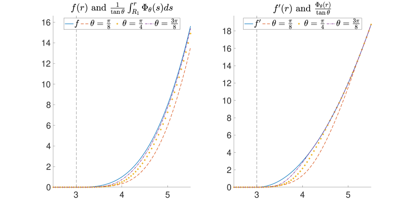
Figure 1.2. Plots of $f(r)$ with $f|_{[0,6]}$ given by (1.7), $f^{\prime}(r)$, $\frac{1}{\tan\theta}\Phi_{\theta}(r)$ (for $d\geq 2$), and $\frac{1}{\tan\theta}\int_{R}^{r}\Phi_{\theta}(r)\,dr$ for $R_{1}=3$.

Figure 1.3. Plots of $f(r)$ given by (1.17), $f^{\prime}(r)$, $\frac{1}{\tan\theta}\Phi_{\theta}(r)$ (for $d\geq 2$), and $\frac{1}{\tan\theta}\int_{R}^{r}\Phi_{\theta}(r)\,dr$ for $R_{1}=3$ and $R_{2}=5$.

Lemma 1.4.

1. For all $\delta>0$, there is $c_{\delta}>0$ such that $\Phi_{\theta}(r)>c_{\delta}\tan\theta$ on $r>R_{1}+\delta$, $\theta>\delta$.

2. $\Phi_{\theta}(r)=f_{\theta}^{\prime}(r)$ if and only if

   (1.12) $$\tan^{2}\theta\geq\frac{r^{2}}{f(r)^{2}}-\frac{2r}{f^{\prime}(r)f(r)}.$$

3. If $f(r)=r$, $f^{\prime}(r)=1$, then $\Phi_{\theta}(r)=f_{\theta}^{\prime}(r)$.

4. For all $\delta>0$, there is $\theta_{\delta}<\pi/2$ such that for $\theta>\theta_{\delta}$, $\Phi_{\theta}(r)=f_{\theta}^{\prime}(r)$ on $r\geq R_{1}+\delta$,

5. The map $(r,\theta)\mapsto\Phi_{\theta}(r)$ is continuous for $(r,\theta)\in[0,\infty)\times(0,\pi/2)$.

Point (1) in Lemma 1.4 implies that, for $R_{{\rm tr}}>R_{1}+\delta$,

(1.13) $$-\int_{R_{1}}^{R_{{\rm tr}}}\Phi_{\theta}(r)\,dr\leq-c_{\delta}(R_{{\rm tr}}-R_{1}-\delta)\tan\theta.$$

Points (1) and (3) in Lemma 1.4 imply that, for $R_{{\rm tr}}>R_{2}$,

(1.14) $$-\int_{R_{1}}^{R_{{\rm tr}}}\Phi_{\theta}(r)\,dr\leq-c_{\delta}(R_{2}-R_{1}-\delta)\tan\theta-(R_{{\rm tr}}-R_{2})\tan\theta<-(R_{{\rm tr}}-R_{2})\tan\theta;$$

Point (4) in Lemma 1.4 implies that for all $\delta>0$ there is $\theta_{\delta}<\pi/2$ such that for $\theta>\theta_{\delta}$,

(1.15) $$-\int_{R_{1}}^{R_{{\rm tr}}}\Phi_{\theta}(r)\,dr\leq-\big{(}f(R_{{\rm tr}})-f(R_{1}+\delta)\big{)}\tan\theta.$$

By (1.13), for $R_{{\rm tr}}>R_{1}+\delta$, the right-hand side of (1.11) is less than or equal to

(1.16) $$C\exp\Big{(}-k\big{(}(2-\eta)c_{\delta}(R_{{\rm tr}}-R_{1}-\delta)\tan\theta-2\Lambda(P,J)\big{)}\Big{)}$$

for some $c_{\delta}>0$; analogous bounds follow using (1.14) and (1.15). These bounds show that the error between $u^{S}$ and $v^{S}$ decreases exponentially in the frequency, the PML width, and the tangent of the scaling angle. In particular, the result (1.8) follows from using (1.16) in (1.11).

An example $f$ that satisfies (1.5) is the piecewise degree-eight polynomial

(1.17) $$f(r)=r\bigg{(}\int_{R_{1}}^{r}(t-R_{1})^{3}(R_{2}-t)^{3}1_{[R_{1},R_{2}]}(t)\,dt\bigg{)}\bigg{(}\int_{R_{1}}^{R_{2}}(t-R_{1})^{3}(R_{2}-t)^{3}\,dt\bigg{)}^{-1};$$

see [BP07, §2]. See Figure 1.3 for plots of $\Phi_{\theta}(r)$ and its integral in this case.

1.3. The main results for black-box scattering

We now describe our results for black-box operators, namely, operators that are equal to the Laplacian outside a ball and are equal to some self-adjoint operator inside the ball; see §2 for a careful definition of these operators and associated notation. Black-box operators (a.k.a. black-box Hamiltonians) include examples such as scattering by Dirichlet, Neumann, and penetrable obstacles, and scattering by inhomogeneous media. Let $R_{0}>0$ and $P:\mathcal{D}\to\mathcal{H}$ be a black-box operator equal to minus the Laplacian outside $B(0,R_{0})$ (i.e., $B(0,R_{0})$ contains the scatterer); here $\mathcal{D}$ is the domain of the operator (see (2.2)) and $\mathcal{H}$ is a Hilbert space coinciding with $L^{2}$ outside $B(0,R_{0})$ (see (2.1)). Let $\chi\in C_{c}^{\infty}(\mathbb{R}^{d})$ with $\chi\equiv 1$ on $B(0,R_{0})$. Then, by [DZ19, Theorem 4.4] (see Proposition 2.1), the cutoff resolvent

$$\chi(P-\lambda^{2})^{-1}\chi:\mathcal{H}\to\mathcal{D},\qquad-\tfrac{\pi}{2}<\operatorname{Arg}(\lambda)<\tfrac{3\pi}{2},$$

is meromorphic with finite rank poles. Let $R_{P}(\lambda):=(P-\lambda^{2})^{-1}$.

The analogue of (1.2) in the black box setting is

(1.18) $$\Lambda(P,J):=\limsup_{\begin{subarray}{c}k\to\infty\\ k\in J\end{subarray}}\frac{1}{k}\log\|\chi R_{P}(k)\chi\|_{\mathcal{H}\to\mathcal{H}}\in[0,\infty].$$

Many black-box Hamiltonians satisfy $\Lambda(P)<\infty$. They include scattering by Dirichlet, Neumann, and penetrable obstacles with smooth boundaries, and scattering by inhomogeneous media with smooth wavespeeds (see §2.1 for details). In addition, for all black-box Hamiltonians satisfying a polynomial bound on the number of eigenvalues of the reference operator (see, e.g., [DZ19, Equation 4.3.10]) and all $\delta>0$, there is a set $J\subset\mathbb{R}$ with $|\mathbb{R}\setminus J|\leq\delta$ such that $\Lambda(P,J)=0$; see [LSW21, Theorem 1.1] or (under an additional assumption about how close the resonances can be to the real axis) [Ste01, Proposition 3].

Let $R_{{\rm tr}}>R_{1}>R_{0}$ and $\Omega_{{\rm tr}}$ bounded and open with Lipschitz boundary such that $B(0,R_{{\rm tr}})\subset\Omega_{{\rm tr}}$, and define $\theta_{0}(P,J,R_{{\rm tr}})$ as in (1.10). We define the complex-scaled operator $P_{\theta}$ corresponding to a black-box Hamiltonian as in (1.4) (for the more general setup, see (A.1)). We then study the difference between the solutions

(1.19) $$(P_{\theta}-k^{2})v=g,\qquad v|_{\Gamma_{{\rm tr}}}=0$$

and

(1.20) $$(P-k^{2})u=g,\qquad(\partial_{r}-ik)u=o(r^{\frac{1-d}{2}})\text{ as }r\to\infty.$$

Theorem 1.5.

Let $J\subset\mathbb{R}$ and $P$ be a black-box Hamiltonian with $\Lambda(P,J)<\infty$. Let $\chi\in C_{c}^{\infty}(B(0,R_{1}))$ with $\chi\equiv 1$ in a neighbourhood of $B(0,R_{0})$, and $\eta,\epsilon>0$. Then there are $C,k_{0}>0$ (independent of $R_{{\rm tr}}$ and $R_{1}$) such that for all $R_{{\rm tr}}>R_{1}+\epsilon$, $B(0,R_{{\rm tr}})\subset\Omega_{{\rm tr}}\subset\mathbb{R}^{d}$ with Lipschitz boundary, $\theta_{0}(P,J,R_{{\rm tr}})+\epsilon<\theta<\pi/2-\epsilon$, $\widetilde{g}\in\mathcal{H}$, $k>k_{0}$, and $k\in J$, the solution $v$ of (1.19) with $g=\chi\widetilde{g}$ exists, is unique, and satisfies

(1.21) $$\|\chi(u-v)\|_{\mathcal{D}}+\|(1-\chi)(u-v)\|_{H^{2}(B(0,R_{1}))}\leq C\exp\bigg{(}-k\Big{(}(2-\eta)\int_{R_{1}}^{R_{{\rm tr}}}\Phi_{\theta}(r)\,dr-2\Lambda(P,J)\Big{)}\bigg{)}\|\widetilde{g}\|_{\mathcal{H}},$$

where $u$ is the solution of  (1.20) with $g=\chi\widetilde{g}$.

One ingredient of the proof of Theorem 1.5 is the following resolvent estimate for (1.19).

Theorem 1.6.

Let $J\subset\mathbb{R}$, $P$ be a black-box Hamiltonian with $\Lambda(P,J)<\infty$, $\chi\in C_{c}^{\infty}(B(0,R_{1}))$ with $\chi\equiv 1$ in a neighbourhood of $B(0,R_{0})$, and $\epsilon>0$. Then there are $C,k_{0}>0$ (independent of $R_{{\rm tr}}$ and $R_{1}$) such that the following holds. For all $R_{{\rm tr}}>R_{1}+\epsilon$, $B(0,R_{{\rm tr}})\subset\Omega_{{\rm tr}}\Subset\mathbb{R}^{d}$ with Lipschitz boundary, $\theta_{0}(P,J,R_{{\rm tr}})+\epsilon<\theta<\pi/2-\epsilon$, all $g\in\mathcal{H}$ with $\operatorname{supp}g\subset\Omega_{{\rm tr}}$, all $k>k_{0}$, and $k\in J$, the solution $v$ to (1.19) exists, is unique, and satisfies

(1.22) $$\|v\|_{\mathcal{H}(\Omega_{{\rm tr}})}+k^{-2}\|v\|_{\mathcal{D}(\Omega_{{\rm tr}})}\leq C\|\chi R_{P}(k)\chi\|_{\mathcal{H}\to\mathcal{H}}\|g\|_{\mathcal{H}},$$

where $\mathcal{H}(\Omega_{{\rm tr}})$ and $\mathcal{D}(\Omega_{{\rm tr}})$ are defined in (3.15).

Another ingredient of the proof of Theorem 1.5 that may be of independent interest is that a bound on the cutoff resolvent $\chi R_{P}\chi$ implies the same bound on the scaled resolvent.

Theorem 1.7.

Suppose $\chi\in C_{c}^{\infty}(B(0,R_{1}))$ with $\chi\equiv 1$ in a neighbourhood of $B(0,R_{0})$. Then, there are $C,k_{0}>0$ such that for $k>k_{0}$, $(P_{\theta}-k^{2})^{-1}:\mathcal{H}\to\mathcal{D}$ exists and satisfies

$$\|(P_{\theta}-k^{2})^{-1}\|_{\mathcal{H}\to\mathcal{H}}+k^{-2}\|(P_{\theta}-k^{2})^{-1}\|_{\mathcal{H}\to\mathcal{D}}\leq C\|\chi R_{P}(k)\chi\|_{\mathcal{H}\to\mathcal{H}}.$$

We also point out that, although it follows the same ideas as the smooth case, complex scaling with $C^{2,\alpha}$ scaling functions as described in Appendix A is new. While the assumption that the scaling function is $C^{2,\alpha}$ is essential for the analysis in Appendix A, and the assumption that it is $C^{3}$ is used to prove resolvent bounds for the free problem via defect measures, other methods of complex scaling exist, see e.g. [AC71, Sim78, Sim79], and apply to, e.g., piecewise linear scaling functions.

Remark 1.8.

In numerical analysis, piecewise linear scaling functions of the form $f_{\theta}(r)=(r-R_{1})_{+}\tan\theta$ are often used (see §1.5). Although our theorems do not apply to this case, we now sketch the key ingredients needed to extend our estimates to this type of scaling function. First, define a modified scaling function $\widetilde{f}_{\theta}(r)$ satisfying (i) $\widetilde{f}_{\theta}(r)=f_{\theta}(r)$ on $r\leq R_{{\rm tr}}$, (ii) for some $R_{3}>R_{{\rm tr}}$, $\theta_{1}>\theta$, $\widetilde{f}_{\theta}(r)\equiv r\tan\theta_{1}$ for $r>R_{3}$, (iii) $\widetilde{f}_{\theta}(r)$ satisfies (1.5) on $\{r>R_{1}\}$, and (iv) $\widetilde{f}_{\theta}\in C^{\infty}(\{r>R_{1}\})$. We would then need two results: first, the nontrapping resolvent estimate for the free problem (i.e., the analogue of Theorem 3.2) and second, agreement of the scaled resolvent and unscaled resolvent away from scaling (see Proposition 3.1). Provided one has these two results, the bounds in Theorems 1.5 and 1.6 follow.

1.4. Ideas and method of proof

PML can be understood as an adaptation (used in numerical analysis) of the method of complex scaling, which originated with [AC71, BC71] and was developed in its modern form for black-box scatterers in [SZ91] (see §3 or [DZ19, §4.5] for an introductory treatment of the subject). In complex scaling, $\mathbb{R}^{d}$ is deformed to a submanifold, $\Gamma_{\theta}\subset\mathbb{C}^{d}$ in such a way that the radiating solutions of (1.1) deform to $L^{2}$ bounded solutions, $u_{\theta}^{S}$, of the deformed problem on $\Gamma_{\theta}:=\{x+if_{\theta}(|x|)\frac{x}{|x|}\}$:

(1.23) $$\begin{cases}(-\Delta_{\Gamma_{\theta}}-k^{2})u^{S}_{\theta}=0&\text{on }\Gamma_{\theta}\setminus\overline{\Omega_{-}}\\ Bu^{S}_{\theta}=-B\exp(ikx\cdot a)&x\in\Gamma_{-}.\\ \end{cases}$$

Moreover this deformation has the property that $u^{S}_{\theta}|_{B(0,R_{1})\setminus\overline{\Omega_{-}}}\equiv u^{S}|_{B(0,R_{1})\setminus\overline{\Omega_{-}}}$. The PML equation (1.3) is then the Dirichlet truncation of (1.23).

Because $u^{S}_{\theta}$ and $u^{S}$ agree on $B(0,R_{1})\setminus\overline{\Omega}_{-}$, we are able to prove Theorem 1.3 by comparing $u_{\theta}^{S}$ and $v^{S}$. The crucial fact (see §4.1) that leads to exponentially good estimates on the error between $u_{\theta}^{S}$ and $v^{S}$ is that both $u_{\theta}^{S}$ and $v^{S}$ are exponentially decaying in $R>R_{1}$ (both in $|x|$ and $k$). Thus, the boundary values for $u_{\theta}^{S}$ on $\Gamma_{{\rm tr}}$ are exponentially small and one can expect that $u_{\theta}^{S}$ and $v^{S}$ are exponentially close. Combining these exponential estimates together with a basic elliptic estimate for $v^{S}$ near $\Gamma_{{\rm tr}}$ and bounds on the cutoff resolvent for (1.23), we can complete the proof of Theorem 1.3. Naively, this argument leads to an exponential improvement $\approx k\int_{R_{1}}^{R_{{\rm tr}}}\Phi_{\theta}(r)\,dr$. To obtain the rate $\approx 2k\int_{R_{1}}^{R}\Phi_{\theta}(r)\,dr$, one must then use that errors near the truncation boundary only propagate with exponential damping toward $R_{1}$. This leads to the second factor in our bound; see the discussion in the caption of Figure 1.4.

To understand the appearance of the function $\Phi_{\theta}(r)$, we recall that the semiclassical principal symbol of $-\hbar^{2}\Delta_{\theta}-1$ (where $\hbar:=1/k$) is

$$p(r,\xi_{r},\omega,\xi_{\omega}):=\Big{(}\frac{\xi_{r}}{1+if_{\theta}^{\prime}(r)}\Big{)}^{2}+\frac{|\xi_{\omega}|_{S^{d-1}}^{2}}{(r+if_{\theta}(r))^{2}}-1.$$

Replacing $\xi_{r}$ by the corresponding operator $\hbar D_{r}$, $(D_{r}:=-i\partial_{r})$, one obtains a family of ODEs in $r$ depending on $|\xi_{\omega}|_{S^{d-1}}^{2}$. The infinitesimal growth/decay of the two possible solutions to this ODE at a point $r$ is then given by the imaginary part of the roots, $s_{+}$ and $s_{-}$, of the polynomial $\xi_{r}\mapsto p(r,\xi_{r},\omega,\xi_{\omega})$. The function $\Phi_{\theta}(r)$ is then given by

$$\Phi_{\theta}(r)=\inf_{|\xi_{\omega}|\geq 0}\min\big{\{}|\operatorname{Im}s_{+}|,|\operatorname{Im}s_{-}|\big{\}};$$

thus it is the smallest possible decay obtained in this way (see Lemma 4.1 for more details).

Figure 1.4. The figure shows a wave $u_{\theta}^{S}$ (in blue) propagating toward $\Gamma_{{\rm tr}}$ from near the obstacle $\Omega_{-}$. The wave $u^{S}_{\theta}$ decays exponentially as it enters the scaling region (where $\Gamma_{\theta}\neq\mathbb{R}^{d}$); this exponential decay is shown in the orange dotted line. The wave $v_{\theta}$ then reflects off $\Gamma_{{\rm tr}}$. There are two possible solutions: one exponentially growing towards the interior and one exponentially decaying towards the interior. Fortunately, the solution exponentially growing towards the interior corresponds to the exponentially decaying (away from the interior) $u^{S}_{\theta}$ and this solution does not produce an error. The exponentially decaying (towards the interior) part of $v_{\theta}$, however, does produce an error in the interior. This solution is again exponentially damped as it travels toward the interior; this solution is shown in red and the decay rate is shown by the brown dashed line.

1.5. Immediate implications for the numerical analysis of the finite-element method with PML truncation

There have been two recent papers on the $k$-explicit analysis of the $h$-version of the finite-element method (FEM) applied to the Helmholtz equation with PML truncation (recall that in the $h$-version of the FEM, convergence is achieved by decreasing the meshwidth $h$ whilst keeping the polynomial degree $p$ constant). The paper [LW19] considers the Helmholtz equation in free space (i.e., with no scatterer) and $f_{\theta}(r)=\sigma_{0}(r-R_{1})_{+}$ (where $x_{+}=x$ for $x\geq 0$ and $=0$ for $x<0$). [CFGT22] considers the Helmholtz equation posed in the exterior of a smooth, starshaped Dirichlet obstacle with $f_{\theta}(r)=r\widetilde{\sigma}/k$ with $\widetilde{\sigma}\in C^{1}$ (and independent of $k$).

For the $h$-FEM applied to the Helmholtz equation, a fundamental question is: how must $h$ decrease with $k$ to maintain accuracy of the Galerkin solution as $k$ increases? Both [LW19] and [CFGT22] prove that, for the PML problems they consider, the answer is the same as for the respective Helmholtz problems truncated with the exact outgoing Dirichlet-to-Neumann map.

Indeed, [LW19, Theorem 4.4] proves that if the approximation spaces consist of piecewise linear polynomials and $hk^{3/2}$ is sufficiently small, then the Galerkin approximation, $v_{h}$, to $v$ satisfying (1.19) (with $P_{\theta}=-\Delta_{\theta}$) exists, is unique, and satisfies

(1.24) $$\|\nabla(v-v_{h})\|_{L^{2}}+k\|v-v_{h}\|_{L^{2}}\leq Chk^{3/2}\|g\|_{L^{2}}$$

(cf. the results in [LSW22] for the Helmholtz problem with the exact outgoing Dirichlet-to-Neumann map). Furthermore, with piecewise polynomial of degree $p$, if $h^{p}k^{p+1}$ is sufficiently small, then [CFGT22, Theorem 5.4] proves that, for the exterior Dirichlet problem with starshaped $\Omega_{-}$, the Galerkin solution exists, is unique, and satisfies a quasioptimal error estimate with quasioptimality constant independent of $k$ (cf. the results in [MS10, MS11] for the Helmholtz exterior Dirichlet problem truncated with the exact outgoing Dirichlet-to-Neumann map).

Combining the results in the present paper with the FEM analysis in [LW19], we immediately have that the results of [LW19] (i.e., existence, uniqueness, and the error bound (1.24) for the Galerkin solution when $hk^{3/2}$ is sufficiently small) extend to the FEM solution of any of the Helmholtz problems in §2.1, provided that (i) $f_{\theta}(r)$ satisfies the assumptions in §1.2, (ii)

$$\|\chi R_{P}(k)\chi\|_{\mathcal{H}\to\mathcal{H}}\leq C/k\quad\text{ for all }k\geq k_{0}$$

(which occurs, for example, when the problem is nontrapping) and (iii) the domain of the PML problem $\mathcal{D}(\Omega_{\rm tr})$, defined by (3.15), equals $H^{2}(\Omega_{\rm tr})$. Indeed, Theorem 1.6 is a generalisation (modulo the differences in scaling functions) of [LW19, Theorem 3.1] and Theorem 1.5 is a generalisation of [LW19, Theorem 3.7].

The results in [CFGT22], however, rely crucially on the fact that $f_{\theta}(r)\sim 1/k$ (e.g., the comparison with the sponge layer in [CFGT22, §5] fails if $f_{\theta}(r)\gg 1/k$); therefore, the results of the present paper cannot be combined with those in [CFGT22]. We expect the error in the PML solution when $f_{\theta}(r)\sim 1/k$ to be only $O(1)$ as $k\rightarrow\infty$. This is in contrast to the exponentially small error when $f_{\theta}(r)\sim 1$ (as shown in Theorem 1.5).

Finally, we highlight that the results of the present paper are used in the follow-up paper [GLSW22] to obtain results about the $hp$-FEM applied to the Helmholtz PML problem; these results are analogous to those obtained in [GLSW21] about the Helmholtz problem truncated with the exact outgoing Dirichlet-to-Neumann map.

1.6. Outline of the paper

§2 recaps the framework of black-box scattering. §3 recaps the method of complex scaling and proves Theorem 1.7. §4 proves elliptic estimates in the scaling region. §5 proves Theorems 1.5 and 1.6 (i.e., the main results in the black-box framework). §6 proves the bound on the relative error in Theorem 1.3 for the plane-wave scattering problem. §7 proves the nontrapping estimate on the free resolvent for the scaled problem with $C^{3}$ scaling function. §A proves results about complex scaling with $C^{2,\alpha}$ scaling function. §B recalls results from semiclassical analysis. §C proves Lemma 1.4 (i.e., properties of $\Phi_{\theta}(r)$).

Acknowledgements

The authors thank Maciej Zworski for several helpful conversations and the anonymous referees for their constructive comments. JG was supported by EPSRC grant EP/V001760/1, and DL and EAS were supported by EPSRC grant EP/R005591/1.

2. Black-box Hamiltonians

Throughout this paper we work in the setting of black-box Hamiltonians (see [DZ19, §4.1]); we now review this notion.

Let $\mathcal{H}$ be a complex Hilbert space with the orthogonal decomposition

(2.1) $$\mathcal{H}=\mathcal{H}_{R_{0}}\oplus L^{2}(\mathbb{R}^{d}\setminus B(0,R_{0})),$$

where $\mathcal{H}_{R_{0}}$ is an arbitrary Hilbert space. We take the standard convention that if $\chi\in L^{\infty}(\mathbb{R}^{d})$ with $\chi\equiv c_{0}\in\mathbb{C}$ on $B(0,R_{0})$, then for $u\in\mathcal{H}$ with $u=u|_{B(0,R_{0})}+u|_{\mathbb{R}^{d}\setminus B(0,R_{0})}$ , $u|_{R_{0}}\in\mathcal{H}_{R_{0}}$, and $u|_{\mathbb{R}^{d}\setminus B(0,R_{0})}\in L^{2}(\mathbb{R}^{d}\setminus B(0,R_{0}))$,

$$\chi u=c_{0}\big{(}u|_{B(0,R_{0})}\big{)}+(\chi|_{\mathbb{R}^{d}\setminus B(0,R_{0})})\big{(}u_{\mathbb{R}^{d}\setminus B(0,R_{0})}\big{)}\in\mathcal{H}.$$

We say that $P$ is a black-box Hamiltonian if, for $\mathcal{H}$ as in (2.1), $P:\mathcal{H}\to\mathcal{H}$ is an unbounded self-adjoint operator with domain $\mathcal{D}\subset\mathcal{H}$ such that

(2.2) $$\begin{gathered}1_{\mathbb{R}^{d}\setminus B(0,R_{0})}\mathcal{D}\subset H^{2}(\mathbb{R}^{d}\setminus B(0,R_{0})),\quad 1_{\mathbb{R}^{d}\setminus B(0,R_{0})}(Pu)=-\Delta\big{(}u|_{\mathbb{R}^{d}\setminus B(0,R_{0})}\big{)},\\ \big{\{}u\in H^{2}(\mathbb{R}^{d})\,:\,u|_{B(0,R_{0}+\epsilon)}\equiv 0\text{ for some }\epsilon>0\big{\}}\subset\mathcal{D},\\ 1_{B(0,R_{0})}(P+i)^{-1}:\mathcal{H}\to\mathcal{H}\text{ is compact}.\end{gathered}$$

We equip $\mathcal{D}$ with the norm

(2.3) $$\|u\|_{\mathcal{D}}^{2}=\|u\|_{\mathcal{H}}^{2}+\|Pu\|_{\mathcal{H}}^{2},\qquad u\in\mathcal{D},$$

and define $\mathcal{D}^{s}$ for $s\in[0,1]$ by interpolation between $\mathcal{H}$ and $\mathcal{D}$. We also define

$$\begin{gathered}\mathcal{H}_{\operatorname{comp}}:=\big{\{}u\in\mathcal{H}\,:\,u|_{\mathbb{R}^{d}\setminus B(0,R_{0})}\in L^{2}_{\operatorname{comp}}\big{\}},\qquad\mathcal{H}_{\operatorname{loc}}:=\mathcal{H}_{R_{0}}\oplus L^{2}_{\operatorname{loc}}(\mathbb{R}^{d}\setminus B(0,R_{0})),\\ \mathcal{D}_{\operatorname{comp}}:=\mathcal{D}\cap\mathcal{H}_{\operatorname{comp}},\qquad\mathcal{D}_{\operatorname{loc}}:=\big{\{}u\in\mathcal{H}_{\operatorname{loc}}\,:\,\chi u\in\mathcal{D},\,\text{for all}\,\chi\in C_{c}^{\infty}(\mathbb{R}^{d}),\,\chi\equiv 1\text{ on }B(0,R_{0})\big{\}}.\end{gathered}$$

We now recall some properties of the resolvent of a black-box Hamiltonian.

Proposition 2.1 (Theorem 4.4 [DZ19]).

Suppose that $P$ is a black-box Hamiltonian. Then,

$$R_{P}(\lambda):=(P-\lambda^{2})^{-1}:\mathcal{H}\to\mathcal{D}\text{ is meromorphic for }\operatorname{Im}\lambda>0$$

with finite rank poles. Moreover, for all $\chi\in C_{c}^{\infty}(\mathbb{R}^{d})$ with $\chi\equiv 1$ on $B(0,R_{0})$,

$$R_{P}(\lambda):\mathcal{H}_{\operatorname{comp}}\to\mathcal{D}_{\operatorname{loc}}\text{ is meromorphic for }-\tfrac{\pi}{2}<\operatorname{Arg}(\lambda)<\tfrac{3\pi}{2},$$

with finite rank poles.

2.1. Examples

1. Scattering by a Dirichlet obstacle. Let $\Omega_{-}\subset\overline{B(0,R_{0})}$ be an open set such that $\Gamma_{-}$ is Lipschitz and $\Omega_{+}:=\mathbb{R}^{d}\setminus\overline{\Omega_{-}}$ is connected. If $\mathcal{H}=L^{2}(\Omega_{+})$ and

   $$\mathcal{D}=\big{\{}u\in H^{1}(\Omega_{+})\,:\,u|_{\Gamma_{-}}=0,\\ ,-\Delta u\in L^{2}(\Omega_{+})\big{\}},$$

   then $P=-\Delta$ is a black-box Hamiltonian by [LSW21, Lemma 2.1]. If $\Gamma_{-}$ is $C^{\infty}$ then by [Bur98, Vod00] $\Lambda(P)<\infty$. If $\Omega_{-}$ is nontrapping [Vai75, MS82] [DZ19, Theorem 4.43], or $\Omega_{-}$ is star shaped [Mor75, CWM08], then $\Lambda(P)=0$.

2. Scattering by a Neumann obstacle. Let $\Omega_{-}\subset\overline{B(0,R_{0})}$ be an open set such that $\Gamma_{-}$ is Lipschitz and $\Omega_{+}:=\mathbb{R}^{d}\setminus\overline{\Omega_{-}}$ is connected. If $\mathcal{H}=L^{2}(\Omega_{+})$ and

   $$\mathcal{D}=\big{\{}u\in H^{1}(\Omega_{+})\,:\,(\partial_{\nu}u)|_{\Gamma_{-}}=0,\,\,-\Delta u\in L^{2}(\Omega_{+})\big{\}},$$

   then $P=-\Delta$ is a black-box Hamiltonian by [LSW21, Lemma 2.1]. If $\Gamma_{-}$ is $C^{\infty}$ then by [Bur98, Vod00] $\Lambda(P)<\infty$. If $\Omega_{-}$ is nontrapping [Vai75, MS82] [DZ19, Theorem 4.43], or $\Gamma_{-}\in C^{3}$ and $\Omega_{-}$ is convex [Mor75], then $\Lambda(P)=0$.

3. Scattering by inhomogeneous media. Let $\alpha>0$, $A\in C^{2,\alpha}(\mathbb{R}^{d};\mathbb{M}_{d\times d})$ be real, symmetric, and positive definite, $b\in C^{1,\alpha}(\mathbb{R}^{d};\mathbb{R}^{d})$, and $c\in C^{0,\alpha}(\mathbb{R}^{d};\mathbb{R})$ with $A|_{\mathbb{R}^{d}\setminus B(0,R_{0})}\equiv I$, $\operatorname{supp}b,\operatorname{supp}c\subset B(0,R_{0})$. If $\mathcal{H}=L^{2}(\mathbb{R}^{d})$ and $\mathcal{D}=H^{2}(\mathbb{R}^{d})$, then

   $$P=\partial_{i}A^{ij}(x)\partial_{j}+(b^{i}(x)D_{i}+D_{i}b^{i}(x))+c(x).$$

   is a black-box Hamiltonian. If the Hamiltonian flow for $A^{ij}\xi_{i}\xi_{j}$ is nontrapping, then $\Lambda(P)=0$ [GSW20]. Moreover, if $A^{ij},b^{i},c\in C^{\infty}$, then $\Lambda(P)<\infty$ [Bur98, Vod00]. We note that we could combine this example with either of Examples 1 and 2, with the result that scattering by an inhomogeneous media contained either a Dirichlet or Neumann obstacle is covered by the black-box framework.

4. Scattering by a penetrable obstacle. Let $\Omega_{-}\subset\overline{B(0,R_{0})}$ be an open set such that $\Gamma_{-}$ is Lipschitz and $\Omega_{+}:=\mathbb{R}^{d}\setminus\overline{\Omega_{-}}$ is connected. Let $A=(A_{-},A_{+})$ with $A_{\pm}\in C^{0,1}(\Omega_{\pm},\mathbb{M}_{d\times d})$ real, symmetric, positive definite, and such that $A|_{\mathbb{R}^{d}\setminus B(0,R_{0})}\equiv I$. Let $c\in L^{\infty}(\Omega_{-})$ be such that $c_{\rm min}\leq c\leq c_{\rm max}$ with $0<c_{\rm min}\leq c_{\rm max}<\infty$, and $\beta>0$. Let $\nu$ be the unit normal vector field on $\partial\Omega_{-}$ pointing from $\Omega_{-}$ into $\Omega_{+}$, and let $\partial_{\nu,A}$ the corresponding conormal derivative from either $\Omega_{-}$ or $\Omega_{+}$. If $\mathcal{H}=L^{2}(\mathbb{R}^{d})$ and

   $$\mathcal{D}:= \Big{\{}v=(v_{-},v_{+})\quad\text{ where }\quad v_{-}\in H^{1}(\Omega_{-}),\quad\nabla\cdot(A_{-}\nabla v_{-})\in L^{2}(\Omega_{-}),$$

   $$\quad v_{+}\in H^{1}\big{(}\mathbb{R}^{d}\setminus\overline{\Omega_{-}}\big{)},\quad\nabla\cdot(A_{+}\nabla v_{+})\big{)}\in L^{2}\big{(}\mathbb{R}^{d}\setminus\overline{\Omega_{-}}\,\big{)},$$

   $$\quad v_{+}=v_{-}\quad\text{ and }\quad\partial_{\nu,A_{+}}v_{+}=\beta\,\partial_{\nu,A_{-}}v_{-}\quad\text{ on }\partial\Omega_{-}\Big{\}},$$

   then

   $$Pv:=-\Big{(}c^{2}\nabla\cdot(A_{-}\nabla v_{-}),\nabla\cdot(A_{+}\nabla v_{+})\Big{)},$$

   is a black-box Hamiltonian by [GLSW21, Lemma 2.4]. If $\partial\Omega_{-}\in C^{\infty}$ and $A_{\pm},c\in C^{\infty}$, then $\Lambda(P)<\infty$ [Bel03].

3. Complex scaling and perfectly matched layers

In §3.1 we review the method of complex scaling; as discussed in the introduction, this plays a crucial role in our analysis of PML. In §3.2 we prove Theorem 1.7. In §3.3 we formulate the PML problem in the black-box framework using the language of complex scaling.

3.1. The scaled operator

Let $R_{2}>R_{1}>R_{0}>0$ and $P$ a black-box Hamiltonian as in (2.2). Let $f_{\theta}\in C^{2,\alpha}([0,\infty);\mathbb{R})$ satisfy

(3.1) $$f_{\theta}(r)\equiv 0\text{ on }r\leq R_{1},\qquad f_{\theta}^{\prime}(r)\geq 0,\qquad f_{\theta}(r)=r\tan\theta\text{ on }r\geq R_{2},$$

and define $\Delta_{\theta}$ as in (1.4). The theory of complex scaling when $f_{\theta}$ is smooth is standard (see [DZ19, §4.5]) but when $f_{\theta}\in C^{2,\alpha}$, some modifications to the standard proofs are required. We record the main outputs of this theory for the operator $\Delta_{\theta}$ here and prove these results (plus necessary intermediate ones) for $C^{2,\alpha}$ scalings in Appendix A.

We now define the complex-scaled operator for a black-box Hamiltonian. With $\chi\in C_{c}^{\infty}(B(0,R_{1}))$ equal to 1 on $B(0,R_{0})$, define $P_{\theta}:\mathcal{H}\to\mathcal{H}$ with domain $\mathcal{D}$ by

(3.2) $$\begin{gathered}P_{\theta}u=P(\chi u)+(-\Delta_{\theta})((1-\chi)u).\end{gathered}$$

(Strictly speaking, the domain and Hilbert space for $P_{\theta}$ involve the scaled manifold; see (A.3) below. However, these can be naturally identified with $\mathcal{D}$ and $\mathcal{H}$, and so in the main body of this paper we make this identification to reduce notation.) The following result is proved in Proposition A.10.

Proposition 3.1.

Let $P_{\theta}$, $\mathcal{D}$, and $\mathcal{H}$, $0\leq\theta<\pi/2$ be as in (3.2). If $\operatorname{Im}(e^{i\theta}\lambda)>0$, then

$$P_{\theta}-\lambda^{2}:\mathcal{D}\to\mathcal{H}$$

is a Fredholm operator of index zero. Moreover, for $R_{0}<R_{1}$ and $\chi\in C_{c}^{\infty}(B(0,R_{1}))$ with $\chi\equiv 1$ on $B(0,R_{0})$,

$${1_{B(0,R_{1})}}(P-\lambda^{2})^{-1}{1_{B(0,R_{1})}}={1_{B(0,R_{1})}}(P_{\theta}-\lambda^{2})^{-1}{1_{B(0,R_{1})}},\qquad\operatorname{Im}(e^{i\theta}\lambda)>0.$$

We also need the following nontrapping estimate on the free resolvent of the scaled problem; since the proof of this result is somewhat long and technical, we postpone the proof to §7.

Theorem 3.2.

Suppose that $f_{\theta}$ is as in (3.1) and $0<\theta<\pi/2$. Then for all $\epsilon>0$ there are $C>0$ and $k_{0}>0$ such that for $k>k_{0}$, $-1\leq m\leq 0$, $0\leq s\leq 2$, and $\epsilon\leq\theta\leq\pi/2-\epsilon$,

$$\|(-\Delta_{\theta}-k^{2})^{-1}\|_{H^{m}\to H^{s+m}}\leq Ck^{s-1}.$$

3.2. From cutoff resolvent estimates estimates to scaled resolvent estimates

We now prove Theorem 1.7; i.e., we show that an estimate on the cutoff resolvent, $\chi R_{P}(\lambda)\chi$, can be transferred to one on $(P_{\theta}-\lambda^{2})^{-1}$. Since most estimates in the literature are stated for the cutoff resolvent, this allows us to directly transfer those estimates to the scaled operator.

Lemma 3.3.

Suppose there are $R>R_{0}$ and $g:[0,\infty)\to(0,\infty]$ such that, for all $\rho\in C_{c}^{\infty}(B(0,R);[0,1])$ with $\rho\equiv 1$ in a neighborhood of $B(0,R_{0})$ and $k>k_{0}$,

(3.3) $$\|\rho R_{P}(k)\rho\|_{\mathcal{H}\to\mathcal{H}}\leq\Upsilon(k).$$

Then, given $\epsilon>0$, there exists $C>0$ such that, for $\epsilon<\theta<\pi/2-\epsilon$, $k>k_{0}$, and $0\leq s\leq 1$, $(P_{\theta}-k^{2})^{-1}:\mathcal{H}\to\mathcal{D}$ exists and satisfies

(3.4) $$\|(P_{\theta}-k^{2})^{-1}\|_{\mathcal{H}\to\mathcal{D}^{s}}\leq Ck^{2s}\Upsilon(k)$$

Theorem 1.7 follows from Lemma 3.3 taking $\Upsilon(k)=\|\chi R_{P}(k)\chi\|_{\mathcal{H}\to\mathcal{H}}$.

Remark 3.4.

Note that one always has $\|\rho R_{P}(k)\rho\|_{\mathcal{H}\to\mathcal{H}}\geq ck^{-1}$. Indeed, given $\rho\in C_{c}^{\infty}(B(0,R);[0,1])$ with $\rho\equiv 1$ in a neighborhood of $B(0,R_{0})$, let $\chi\in C_{c}^{\infty}(B(0,R)\setminus B(0,R_{0}))$ with $\operatorname{supp}\chi\subset\{\rho\equiv 1\}$. Let $u=\chi e^{ikx\cdot a}$ for some $a\in\mathbb{R}^{d}$ with $|a|=1$. Then, for some $C_{1},C_{2}>0$ (independent of $k$),

$$\|(P-k^{2})u\|_{\mathcal{H}}=\|(-\Delta-k^{2})u\|_{L^{2}}=\|[-\Delta,\chi]e^{ikx\cdot a}\|_{L^{2}}=\|(2ik\langle\partial\chi,a\rangle+\Delta\chi)e^{ikx\cdot a}\|_{L^{2}}\leq C_{1}k,$$

and $\|u\|_{\mathcal{H}}\geq C_{2}$. Therefore, since $\operatorname{supp}\chi\subset\{\rho\equiv 1\}$,

$$\|\rho R_{P}(k)\rho(P-k^{2})u\|_{\mathcal{H}}=\|\rho u\|_{\mathcal{H}}\geq\|u\|_{\mathcal{H}}\geq(C_{2}/C_{1})k^{-1}\|(P-k^{2})u\|_{\mathcal{H}}.$$

Proof of Lemma 3.3.

By Proposition 3.1, $P_{\theta}-k^{2}$ is Fredholm of index zero; thus existence of $(P_{\theta}-k^{2})^{-1}$ follows from injectivity, and injectivity follows once we establish the a priori bound (3.4).

The idea of the proof of (3.4) is to approximate $(P_{\theta}-k^{2})^{-1}$ away from the black-box using the free scaled resolvent, and near the black-box using the unscaled resolvent. Let $\widetilde{R}:=\min(R,R_{1})$, $f\in\mathcal{H}$ and $\chi_{0},\chi_{1}\in C_{c}^{\infty}(B(0,\widetilde{R}))$ with $\chi_{1}\equiv 1$ in a neighborhood of $\operatorname{supp}\chi_{0}$ and $\chi_{0}\equiv 1$ in a neighborhood of $B(0,R_{0})$. Let $u=(P_{\theta}-k^{2})^{-1}g$ and $v=(-\Delta_{\theta}-k^{2})^{-1}(1-\chi_{1})g$. Then, we define

$$(P_{\theta}-k^{2})(u-(1-\chi_{0})v)=g+[-\Delta,\chi_{0}]v-(1-\chi_{0})(1-\chi_{1})g=\chi_{1}g+[-\Delta,\chi_{0}]v=:\widetilde{g}$$

and observe that $\widetilde{g}$ satisfies $\operatorname{supp}\widetilde{g}\Subset B(0,\widetilde{R})$. Let $\widetilde{u}=(P_{\theta}-k^{2})^{-1}\widetilde{g}$ so that $u=\widetilde{u}+(1-\chi_{0})v$. By Theorem 3.2,

(3.5) $$\|u-\widetilde{u}\|_{\mathcal{H}}=\|(1-\chi_{0})(-\Delta_{\theta}-k^{2})^{-1}(1-\chi_{1})g\|_{\mathcal{H}}\leq Ck^{-1}\|g\|_{\mathcal{H}}.$$

Therefore, we need only estimate $\widetilde{u}$. By Theorem 3.2 with $m=0$ and $s=1$,

(3.6) $$\|\widetilde{g}\|_{\mathcal{H}}\leq\|\chi_{1}g\|_{\mathcal{H}}+\|[-\Delta,\chi_{0}]v\|_{L^{2}}\leq\|g\|_{\mathcal{H}}+\|[-\Delta,\chi_{0}](-\Delta_{\theta}-k^{2})^{-1}(1-\chi_{1})g\|_{L^{2}}\leq C\|g\|_{\mathcal{H}}.$$

Since $\operatorname{supp}\widetilde{g}\Subset B(0,\widetilde{R})$, there is $\rho\in C_{c}^{\infty}(B(0,\widetilde{R}))$ such that $\rho\equiv 1$ on $\operatorname{supp}\widetilde{g}\cup B(0,R_{0})$ and hence

$$\widetilde{u}=(P_{\theta}-k^{2})^{-1}\rho\widetilde{g}.$$

Let $\rho_{1}\in C_{c}^{\infty}(B(0,\widetilde{R}))$ with $\rho_{1}\equiv 1$ in a neighborhood of $\operatorname{supp}\rho$. Then,

$$(-\Delta_{\theta}-k^{2})(1-\rho_{1})\widetilde{u}=(1-\rho_{1})\rho\widetilde{g}-[-\Delta,\rho_{1}]\widetilde{u}=[\rho_{1},-\Delta]\widetilde{u},$$

and thus

$$(1-\rho_{1})\widetilde{u}=(-\Delta_{\theta}-k^{2})^{-1}[\rho_{1},-\Delta]\widetilde{u}.$$

Therefore, for $\rho_{2}\in C_{c}^{\infty}(B(0,\widetilde{R})\setminus B(0,R_{0}))$ with $\rho_{2}\equiv 1$ on $\operatorname{supp}\partial\rho_{1}$, and $\rho_{3}\in C_{c}^{\infty}(B(0,\widetilde{R}))$ with $\rho_{3}\equiv 1$ on $\operatorname{supp}\rho_{2}\cup\operatorname{supp}\rho_{1}$,

$$\|(1-\rho_{1})\widetilde{u}\|_{L^{2}}=\|(-\Delta_{\theta}-k^{2})^{-1}[\rho_{1},-\Delta]\rho_{2}\widetilde{u}\|_{L^{2}}\leq C\|\rho_{2}\widetilde{u}\|_{L^{2}} =C\|\rho_{2}\rho_{3}(P_{\theta}-k^{2})^{-1}\rho_{3}\rho\widetilde{g}\|_{\mathcal{H}}$$

$$=C\|\rho_{2}\rho_{3}R_{P}(k)\rho_{3}\rho\widetilde{g}\|_{\mathcal{H}}$$

$$\leq C\Upsilon(k)\|\rho\widetilde{g}\|_{\mathcal{H}}\leq C\Upsilon(k)\|\widetilde{g}\|_{\mathcal{H}},$$

where we have used Theorem 3.2 (with $m=-1$ and $s=1$), Proposition 3.1, and the assumption (3.3). Putting this together with

$$\|\rho_{1}\widetilde{u}\|_{\mathcal{H}}=\|\rho_{1}\rho_{3}\widetilde{u}\|_{\mathcal{H}}\leq\|\rho_{3}(P_{\theta}-k^{2})^{-1}\rho_{3}\rho\widetilde{g}\|_{\mathcal{H}}=\|\rho_{3}R_{P}(k)\rho_{3}\rho\widetilde{g}\|_{\mathcal{H}}\leq\Upsilon(k)\|\rho\widetilde{g}\|_{\mathcal{H}}\leq\Upsilon(k)\|\widetilde{g}\|_{\mathcal{H}},$$

we have

$$\|\widetilde{u}\|_{\mathcal{H}} \leq C\Upsilon(k)\|\widetilde{g}\|_{\mathcal{H}}.$$

Finally, using (3.5) and (3.6) and the fact that $\Upsilon(k)>ck^{-1}$ (by Remark 3.4) completes the proof of (3.4) for $s=0$.

By the definition of $\|\cdot\|_{\mathcal{D}}$ (2.3), to obtain the estimate for $s=1$, we need to bound $\|Pu\|_{\mathcal{H}}$. Let $\psi_{i}\in C_{c}^{\infty}(B(0,R_{1}))$, $i=-1,0,1$ with $\psi_{i}\equiv 1$ in a neighborhood of $B(0,R_{0})$, and $\operatorname{supp}\psi_{i}\subset\{\psi_{i+1}\equiv 1\}$. It is then sufficient to bound $\|P\psi_{1}u\|_{\mathcal{H}}$ and $\|(1-\psi_{0})u\|_{H^{2}}$. Now, since $P=P_{\theta}$ on $B(0,R_{1})$,

(3.7) $$P{\psi_{1}}u=k^{2}\psi_{1}u+\psi_{1}g+[-\Delta,\psi_{1}]u,$$

and

$$(-\Delta_{\theta}-k^{2})(1-\psi_{0})u=[\Delta,\psi_{0}]u+(1-\psi_{0})g.$$

A priori, we only have $u\in\mathcal{H}$, and thus the right-hand side of the last equation is, a priori, only in $H^{-1}$. By two applications of Theorem 3.2 (the first with $m=-1$ and $s=2$ and the second with $m=0$ and $s=1$),

(3.8) $$\|(1-\psi_{0})u\|_{H^{1}}\leq Ck\|u\|_{\mathcal{H}}+C\|g\|_{\mathcal{H}}.$$

Since

$$\|[-\Delta,\psi_{1}]u\|_{L^{2}}\leq C\|(1-\psi_{0})u\|_{H^{1}},$$

using these last two inequalities in (3.7), along with (3.4) with $s=0$ (which we established above), we have

(3.9) $$\|P\psi_{1}u\|_{\mathcal{H}}\leq C\big{(}k^{2}\|u\|_{\mathcal{H}}+\|g\|_{\mathcal{H}}\big{)}\leq Ck^{2}\big{(}\Upsilon(k)+k^{-2}\big{)}\|g\|_{\mathcal{H}},$$

which is the required estimate on $\|P\psi_{1}u\|_{\mathcal{H}}$; we therefore only need to bound $\|(1-\psi_{0})u\|_{H^{2}}$. If we can show that $\Delta_{\theta}((1-\psi_{0})u)\in L^{2}$, then, by elliptic regularity (since $\Delta_{\theta}$ is elliptic by [DZ19, Theorem 4.32]),

(3.10) $$\|(1-\psi_{0})u\|_{H^{2}}\leq C\big{(}\|\Delta_{\theta}(1-\psi_{0})u\|_{L^{2}}+\|u\|_{\mathcal{H}}\big{)},$$

with a uniform constant for $\theta\in[\epsilon,\pi/2-\epsilon]$. Now

(3.11) $$\Delta_{\theta}((1-\psi_{0})u)=(1-\psi_{0})(k^{2}u+g)-[\Delta_{\theta},\psi_{0}]u,$$

(3.12) $$\|[\Delta_{\theta},\psi_{0}]u\|_{L^{2}}=\|[\Delta,\psi_{0}]u\|_{L^{2}}\leq C\|(1-\psi_{-1})u\|_{H^{1}},$$

and exactly the same argument used to prove (3.8) shows that

(3.13) $$\|(1-\psi_{-1})u\|_{H^{1}}\leq Ck\|u\|_{\mathcal{H}}+C\|g\|_{\mathcal{H}}.$$

Therefore, combining (3.10)–(3.13), and using the bound (3.4) with $s=0$, we obtain that

(3.14) $$\|(1-\psi_{0})u\|_{H^{2}}\leq C\big{(}k^{2}\|u\|_{\mathcal{H}}+\|g\|_{\mathcal{H}}\big{)}\leq Ck^{2}\big{(}\Upsilon(k)+k^{-2}\big{)}\|g\|_{\mathcal{H}}.$$

The combination of (3.9) and (3.14) proves the bound (3.4) for $s=1$; the bound (3.4) for $0<s<1$ then follows by interpolation. ∎

3.3. The PML operator

In addition to the Fredholm property for $P_{\theta}$, we need Fredholm properties for the corresponding PML operator. Let $\Omega_{{\rm tr}}\Subset\mathbb{R}^{d}$ have Lipschitz boundary and $B(0,R_{1})\subset\Omega_{{\rm tr}}$. We study the PML operator $P^{D}_{\theta}-\lambda^{2}$ on $\Omega_{{\rm tr}}$. That is, we define

(3.15) $$\begin{gathered}\mathcal{H}(\Omega_{{\rm tr}}):=\mathcal{H}_{R_{0}}\oplus L^{2}(\Omega_{{\rm tr}}\setminus B(0,R_{0})),\\ \mathcal{D}(\Omega_{{\rm tr}}):=\Big{\{}u\in\mathcal{H}(\Omega_{{\rm tr}})\,:\,{\text{for all}\,\chi\in C_{c}^{\infty}(B(0,R_{1})),\,\chi\equiv 1\text{ on }B(0,R_{0}),}\\ \hskip 85.35826pt\chi u\in\mathcal{D},\,{(1-\chi)u\in H_{0}^{1}(\Omega_{{\rm tr}}),\,-\Delta_{\theta}((1-\chi)u)\in L^{2}(\Omega_{{\rm tr}})}\Big{\}},\\ P^{D}_{\theta}u:=P(\chi u)+(-\Delta_{\theta})((1-\chi)u).\end{gathered}$$

We then consider $P^{D}_{\theta}:\mathcal{H}(\Omega_{{\rm tr}})\to\mathcal{H}(\Omega_{{\rm tr}})$ with domain $\mathcal{D}(\Omega_{{\rm tr}})$ and norm

(3.16) $$\|u\|_{\mathcal{D}(\Omega_{\rm tr})}^{2}=\|u\|_{\mathcal{H}(\Omega_{\rm tr})}^{2}+\|P_{\theta}^{D}u\|_{\mathcal{H}(\Omega_{\rm tr})}^{2},\qquad u\in\mathcal{D}(\Omega_{\rm tr}).$$

Proposition 3.5.

Let $P^{D}_{\theta}$, $\mathcal{H}(\Omega_{{\rm tr}})$, and $\mathcal{D}(\Omega_{{\rm tr}})$ be as in (3.15). Then, $P^{D}_{\theta}-\lambda^{2}:\mathcal{D}(\Omega_{\rm tr})\to\mathcal{H}(\Omega_{{\rm tr}})$ is Fredholm with index zero.

Proposition 3.5 is proved in Appendix A; see Proposition A.12.

4. Elliptic estimates

In this section, we prove the necessary bounds on the solutions to $(P_{\theta}-k^{2})u=f$ and $(P^{D}_{\theta}-k^{2})v=f$ for $k\in\mathbb{R}$, $k\gg 1$. The Carleman estimates in §4.1 describe how both $u$ and $v$ propagate in the scaling region. The bound in §4.2 (obtained essentially by integration by parts) describes the behaviour of $v$ in a neighbourhood of $\Gamma_{\rm tr}$.

It is convenient to use the semiclassical rescaling $\hbar=k^{-1}$ and write these equations as

$$(\hbar^{2}P_{\theta}-1)u=\hbar^{2}g,\qquad(\hbar^{2}P_{\theta}^{D}-1)v=\hbar^{2}g,$$

and we do so throughout the rest of the paper. We use the semiclassically-scaled Sobolev norms for $\ell\in\mathbb{N}$ defined by

$$\|u\|_{H_{\hbar}^{\ell}}^{2}:=\sum_{|\alpha|\leq\ell}\|(\hbar D)^{\alpha}u\|_{L^{2}}^{2},$$

where $D:=-i\partial$. Then, for $\ell\in\mathbb{N}$, $H_{\hbar}^{-\ell}=(H_{\hbar}^{\ell})^{*}$ and the norms for $s\in\mathbb{R}$ are defined by interpolation. With $\langle\cdot\rangle:=(1+|\cdot|^{2})^{1/2}$, these norms satisfy

$$\|u\|_{H_{\hbar}^{s}}\sim\|\langle\hbar D\rangle^{s}u\|_{L^{2}}.$$

4.1. Carleman estimates

We start by proving an exponential estimate for solutions to

$$(-\hbar^{2}\Delta_{\theta}-1)u=g,$$

for $u$ supported in $r>R_{1}$. Our estimates are proved using Carleman estimates with weight $\psi=\psi(r)$. To this end, for $\psi\in C^{\infty}([0,\infty))$, we define

(4.1) $$P_{\psi}:=e^{\psi/\hbar}(-\hbar^{2}\Delta_{\theta}-1)e^{-\psi/\hbar},$$

with semiclassical principal symbol

$$p_{\psi}(r,\omega,\xi_{r},\xi_{\omega}):=\Big{(}\frac{\xi_{r}+i\psi^{\prime}}{1+if_{\theta}^{\prime}(r)}\Big{)}^{2}+\frac{|\xi_{\omega}|^{2}_{S^{d-1}}}{(r+if_{\theta}(r))^{2}}-1.$$

Lemma 4.1.

Let $\epsilon>0$ and $\Phi_{\theta}$ be as in (1.9). Then there is $c_{\epsilon,f}>0$ such that for $r>R_{1}+\epsilon$ and $\epsilon\leq\theta\leq\pi/2-\epsilon$, $\Phi_{\theta}(r)>c_{\epsilon,f}$. Moreover, given $0\leq a<1$, there is $c>0$ such that for all $\epsilon\leq\theta\leq\pi/2-\epsilon$ and $r\geq R_{1}+\epsilon$ such that

(4.2) $$|\psi^{\prime}(r)|<a\Phi_{\theta}(r),$$

$P_{\psi}$ is uniformly semiclassically elliptic in $r\geq R_{1}+\epsilon$; i.e.,

$$|p_{\psi}|\geq c\langle\xi\rangle^{2},\qquad r\geq R_{1}+\epsilon.$$

Proof.

In the following arguments, $c_{f,\epsilon},C_{f,\epsilon}>0$ are constants depending on $f$ and $\epsilon$ whose values may change from line to line. Throughout the proof, $r>R_{1}+\epsilon$ and $\theta\in[\epsilon,\pi/2-\epsilon]$.

The solutions, $s_{\pm}$ to

$$\widetilde{p}(s):=\Big{(}\frac{s}{1+if_{\theta}^{\prime}(r)}\Big{)}^{2}+\frac{|\xi_{\omega}|^{2}}{(r+if_{\theta}(r))^{2}}-1=0$$

are given by

$$s_{\pm}=\pm(1+if_{\theta}^{\prime}(r))\sqrt{1-\frac{|\xi_{\omega}|^{2}}{(r+if_{\theta}(r))^{2}}}.$$

The definition of $\Phi_{\theta}(r)$ (1.9) then implies that

(4.3) $$\Phi_{\theta}(r)=\inf_{|\xi_{\omega}|\geq 0}\min\big{\{}|\operatorname{Im}s_{+}|,|\operatorname{Im}s_{-}|\big{\}}=\inf_{|\xi_{\omega}|\geq 0|\operatorname{Im}s_{+}|,}$$

since $s_{+}=-s_{-}$.

By considering the real and imaginary parts of $\widetilde{p}(s)$, we find that

$$|\widetilde{p}(s)|\geq c_{f,\epsilon}\big{(}|\operatorname{Re}s|^{2}+|\xi_{\omega}|^{2}{/r^{2}}+1\big{)},\qquad\operatorname{Im}s=0,$$

where we have used the particular form of $f_{\theta}(r)$, i.e., $f_{\theta}(r)=f(r)\tan\theta$ and the fact that $\theta\in[\epsilon,\pi/2-\epsilon]$ to get uniformity in $\theta$. Therefore, since there exists $c_{f,\epsilon}>0$ such that,

$$|\partial_{s}\widetilde{p}|\leq c_{f,\epsilon}|s|,$$

there is $c_{f,\epsilon}>0$ such that

(4.4) $$|\widetilde{p}(s)|\geq c_{f,\epsilon}\big{(}|\operatorname{Re}s|^{2}+|\xi_{\omega}|^{2}{/r^{2}}+1\big{)},\qquad|\operatorname{Im}s|\leq c_{f,\epsilon},$$

and thus $|\operatorname{Im}s_{\pm}|>c_{f,\epsilon}$. Therefore, by (4.3), $\Phi_{\theta}(r)>c_{f,\epsilon}$. Hence, if $|\operatorname{Im}s|<a\Phi_{\theta}(r)$, then

$$\min_{\pm}|s-s_{\pm}|>c_{f,\epsilon}(1-a).$$

In particular, since

$$|\partial_{s}\widetilde{p}(s_{\pm})|=\Big{|}\frac{2s_{\pm}}{(1+if_{\theta}^{\prime}(r))^{2}}\Big{|}\geq c_{f,\epsilon},$$

and

$$|\partial_{s}^{2}\widetilde{p}(s)|=\frac{1}{|1+if_{\theta}^{\prime}|^{2}}\leq C_{f,\epsilon},$$

there is $c_{a,f,\epsilon}>0$ such that

$$|\widetilde{p}(s)|\geq c_{a,f,\epsilon}$$

if $|\operatorname{Im}s|<a\Phi_{\theta}(r)$. Finally, by considering the real and imaginary parts of $\widetilde{p}(s)$ again (this time with $s$ not necessarily real), we see that there exists $C_{f,\epsilon}>0$ such that, for $|\operatorname{Re}s|^{2}+|\xi_{\omega}|^{2}/r^{2}\geq C_{f,\epsilon}$,

$$|\widetilde{p}(s)|\geq C_{f,\epsilon}^{-1}\big{(}|\operatorname{Re}s|^{2}+|\xi_{\omega}|^{2}/r^{2}+1\big{)}.$$

Together, we have shown that for $|\operatorname{Im}s|<a\Phi_{\theta}(r)$,

$$|\widetilde{p}(s)|\geq c_{a,f,\epsilon}\big{(}|\operatorname{Re}s|^{2}+|\xi_{\omega}|^{2}/r^{2}+1\big{)}$$

and the claim follows. ∎

In the rest of the paper we use the notation that $(a,b)_{r}:=B(0,b)\setminus B(0,a)$.

Lemma 4.2.

Let $\epsilon>0$, $\eta>0$. Then there are $C>0$, $\hbar_{0}>0$, and $0<\widetilde{\eta}<\epsilon/6$ such that for all $\epsilon\leq\theta\leq\pi/2-\epsilon$, $\delta>\epsilon$, $u\in L^{2}$, $0<\hbar<\hbar_{0}$,

(4.5) $$\|u\|_{H_{\hbar}^{2}(R_{1}+\delta-2\widetilde{\eta},R_{1}+\delta-\widetilde{\eta})_{r}}\leq C\|(-\hbar^{2}\Delta_{\theta}-1)u\|_{L^{2}(R_{1},R_{1}+\delta)_{r}}\\ +C\exp\Big{(}-\frac{(1-\eta)}{\hbar}\int_{R_{1}}^{R_{1}+\delta}\Phi_{\theta}(s)\,ds\Big{)}\hbar\|u\|_{H_{\hbar}^{1}(R_{1},R_{1}+\widetilde{\eta})_{r}}+C\hbar\|u\|_{H_{\hbar}^{1}(R_{1}+\delta-\widetilde{\eta},R_{1}+\delta)_{r}},$$

and

(4.6) $$\|u\|_{H_{\hbar}^{2}(R_{1}+\delta-2\widetilde{\eta},\infty)_{r}}\leq C\|(-\hbar^{2}\Delta_{\theta}-1)u\|_{L^{2}(R_{1},\infty)_{r}}\\ +C\exp\Big{(}-\frac{(1-\eta)}{\hbar}\int_{R_{1}}^{R_{1}+\delta}\Phi_{\theta}(s)\,ds\Big{)}\hbar\|u\|_{H_{\hbar}^{1}(R_{1},R_{1}+\widetilde{\eta})_{r}}.$$

Proof.

Let $P_{\psi}$ be as in (4.1). To prove the lemma, we construct a $\psi$ satisfying (4.2) with $a=1-\widetilde{\eta}$ for some, not yet specified, $\widetilde{\eta}$. Let $\psi_{0}\in C_{c}^{\infty}((2\widetilde{\eta},\delta-2\widetilde{\eta});[0,1])$ with $\psi_{0}\equiv 1$ on $(3\widetilde{\eta},\delta-3\widetilde{\eta})$. Then, let $0\leq\widetilde{\Phi}_{\theta}(r)\in C^{\infty}$ with $(1-{2}\widetilde{\eta})\Phi_{\theta}(r)\leq\widetilde{\Phi}_{\theta}(r)\leq{(1-\widetilde{\eta})}\Phi_{\theta}(r)$ on $[R_{1}+\widetilde{\eta},\infty)$ and $\operatorname{supp}\widetilde{\Phi}_{\theta}\subset(R_{1}+\widetilde{\eta}/2,\infty)$. Then define

(4.7) $$\psi(t)=-\int_{t}^{\infty}\widetilde{\Phi}_{\theta}(s)\psi_{0}(s-R_{1})\,ds,$$

and choose $0<\widetilde{\eta}<\epsilon/6$ small enough such that

(4.8) $$-\int_{-\infty}^{\infty}\widetilde{\Phi}_{\theta}(s){\psi_{0}}(s-R_{1})\,ds\leq-(1-\eta)\int_{R_{1}}^{R_{1}+\delta}\Phi_{\theta}(s)\,ds;$$

note that this choice can be made uniformly in $\delta>\epsilon$. By (4.7) and the support properties of $\psi_{0}$,

$$|\psi^{\prime}(t)|=\widetilde{\Phi}_{\theta}(t)|{\psi_{0}}(t-R_{1})|\leq(1-\widetilde{\eta})\Phi_{\theta}(t),$$

so that, by Lemma 4.1, $|p_{\psi}|\geq c\langle\xi\rangle^{2}$, for all $t$. In addition

(4.9) $$\psi(t)=-\int_{-\infty}^{\infty}\widetilde{\Phi}_{\theta}(s){\psi_{0}}(s-R_{1})\,ds,\,\,t-R_{1}\leq 2\widetilde{\eta},\quad\text{ and }\quad\psi(t)=0,\,\,t-R_{1}\geq\delta-2\widetilde{\eta},$$

see Figure 4.1, and

$$|\partial^{\alpha}\psi(t)|\leq C_{\alpha\widetilde{\eta}\epsilon}\quad{\text{ for all }t}.$$

To prove (4.5), let $\chi_{1},\chi_{2}\in C_{c}^{\infty}(R,R+\delta)$ with $\chi_{1}\equiv 1$ in a neighborhood of $[R_{1}+\widetilde{\eta},R_{1}+\delta-\widetilde{\eta}]$, $\chi_{2}\equiv 1$ on $\operatorname{supp}\chi_{1}$. Let $\chi_{-}\in C_{c}^{\infty}(R_{1},R_{1}+\widetilde{\eta})$, $\chi_{+}\in C_{c}^{\infty}(R_{1}+\delta-\widetilde{\eta},R+\delta)$ with $\chi_{-}+\chi_{+}\equiv 1$ on $\operatorname{supp}(\chi_{2}-\chi_{1})$; see Figure 4.1.

Figure 4.1. The cut-off functions and behaviour of the function $\psi(t)$ in the proof of Lemma 4.2. Although $\widetilde{\eta}$ appears large here (for readability), we emphasise that $\widetilde{\eta}\ll\delta$.

Now,

$$P_{\psi}=\operatorname{Op}_{\hbar}(p_{0,\psi})+\hbar\operatorname{Op}_{\hbar}(p_{1,\psi}).$$

with $p_{0,\psi}\in C^{1,\alpha}S^{2}$, $p_{1,\psi}\in C^{0,\alpha}S^{1}$, and

$$|p_{0,\psi}|\geq c_{\epsilon\widetilde{\eta}}\langle\xi\rangle^{2}.$$

Let $\rho=\frac{1}{1+\alpha}$. Then, by Lemmas B.6 and B.7, there is $p_{\hbar,\psi}$ satisfying

$$|\partial_{x}^{\gamma}\partial_{\xi}^{\beta}p_{\hbar,\psi}(x,\xi)|\leq C_{\epsilon\widetilde{\eta}\gamma\beta}\hbar^{-\rho\gamma}\langle\xi\rangle^{m-|\beta|+\rho\gamma},$$

and

$$\|\operatorname{Op}_{\hbar}(p_{\hbar,\psi})-P_{\psi}\|_{H_{\hbar}^{1}\to L^{2}}\leq C_{\epsilon\widetilde{\eta}}\hbar.$$

By a standard elliptic-parametrix construction for $p_{\hbar}$ in an exotic symbol class (see Theorem B.2 for the standard elliptic-parametrix construction and [Tay96, §7.3-7.4] for the construction in exotic calculi), there is $E:L^{2}\to H_{\hbar}^{2}$, such that

$$\chi_{1}=E\operatorname{Op}_{\hbar}(p_{\hbar,\psi})+O(\hbar^{\infty})_{\Psi^{-\infty}}.$$

Moreover, both $E$ and the error are uniform over $\delta\geq\epsilon$, $\epsilon\leq\theta\leq\pi/2-\epsilon$. Therefore,

(4.10) $$\chi_{1}e^{\psi/\hbar}u =\chi_{1}\chi_{2}e^{\psi/\hbar}u=E\operatorname{Op}_{\hbar}(p_{\hbar,\psi})\chi_{2}e^{\psi/\hbar}u+O_{\widetilde{\eta}\epsilon}(\hbar^{\infty})_{\Psi^{-\infty}}\chi_{2}e^{\psi/\hbar}u$$

$$=E(P_{\psi}+(\operatorname{Op}_{\hbar}(p_{\hbar,\psi})-P_{\psi}))\chi_{2}e^{\psi/\hbar}u+O_{\widetilde{\eta}\epsilon}(\hbar^{\infty})_{\Psi^{-\infty}}\chi_{2}e^{\psi/\hbar}u$$

$$=E\chi_{2}e^{\psi/\hbar}g-Ee^{\psi/\hbar}[\hbar^{2}\Delta_{\theta},\chi_{2}]u+O_{\widetilde{\eta}\epsilon}(\hbar)_{H_{\hbar}^{1}\to H_{\hbar}^{2}}\chi_{2}e^{\psi/\hbar}u,$$

where $f:=(-\hbar^{2}\Delta_{\theta}-1)u.$ Therefore, since $\partial\chi_{2}$ is supported where $\chi_{+}+\chi_{-}=1$,

(4.11) $$\|\chi_{1}e^{\psi/\hbar}u\|_{H_{\hbar}^{2}}\leq C\|\chi_{2}e^{\psi/\hbar}g\|_{L^{2}}+C\hbar\|\chi_{-}e^{\psi/\hbar}u\|_{H_{\hbar}^{1}}+C\hbar\|\chi_{+}e^{\psi/\hbar}u\|_{H_{\hbar}^{1}}+C\hbar\|\chi_{2}e^{\psi/\hbar}u\|_{H_{\hbar}^{1}}.$$

Since $\chi_{2}=(\chi_{2}-\chi_{1})+\chi_{1}$ and $\chi_{+}+\chi_{-}=1$ on $\operatorname{supp}(\chi_{2}-\chi_{1})$,

(4.12) $$\|\chi_{2}e^{\psi/\hbar}u\|_{H^{1}_{\hbar}}\leq C\|\chi_{-}e^{\psi/\hbar}u\|_{H^{1}_{\hbar}}+C\|\chi_{+}e^{\psi/\hbar}u\|_{H^{1}_{\hbar}}+\|\chi_{1}e^{\psi/\hbar}u\|_{H^{1}_{\hbar}}.$$

Combining (4.11) and (4.12) and taking $\hbar$ sufficiently small (depending only on $\eta$ and $\epsilon$), we have

(4.13) $$\|\chi_{1}e^{\psi/\hbar}u\|_{H^{2}_{\hbar}}\leq C\|\chi_{2}e^{\psi/\hbar}g\|_{L^{2}}+C\hbar\|\chi_{-}e^{\psi/\hbar}u\|_{H_{\hbar}^{1}}+C\hbar\|\chi_{+}e^{\psi/\hbar}u\|_{H_{\hbar}^{1}}.$$

Then, since $\psi\leq-(1-\eta)\int_{R_{1}}^{R_{1}+\delta}\Phi_{\theta}(s)ds$ on $\operatorname{supp}\chi_{-}$ (by (4.8) and (4.9); see Figure 4.1), and $\psi\leq 0$ everywhere (and thus, in particular, on $\operatorname{supp}\chi_{+}$),

$$\|\chi_{1}e^{\psi/\hbar}u\|_{H_{\hbar}^{2}}\leq C\|\chi_{2}e^{\psi/\hbar}g\|_{L^{2}}+C\exp\Big{(}-\frac{(1-\eta)}{\hbar}\int_{R_{1}}^{R_{1}+\delta}\Phi_{\theta}(s)ds\Big{)}\hbar\|\chi_{-}u\|_{H_{\hbar}^{1}}+C\hbar\|\chi_{+}u\|_{H_{\hbar}^{1}}.$$

The lemma now follows since $\chi_{1}\equiv 1$ and $\psi\equiv 0$ on $(R_{1}+\delta-2\widetilde{\eta},R_{1}+\delta-\widetilde{\eta})$, $\operatorname{supp}\chi_{-}\subset(R_{1},R_{1}+\widetilde{\eta})$, and $\operatorname{supp}\chi_{+}\subset(R_{1}+\delta-\widetilde{\eta},R_{1}+\delta)$, and $\psi\leq 0$ everywhere.

To prove (4.6), we make the same argument as above except that $\chi_{1},\chi_{2}\in C^{\infty}(R_{1},\infty)$ with $\chi_{1}\equiv 1$ in a neighborhood of $[R_{1}+\widetilde{\eta},\infty)$, $\chi_{2}\equiv 1$ on $\operatorname{supp}\chi_{1}$, and $\chi_{+}=0$. ∎

Next, we need an elliptic estimate away from the support of the right hand side.

Lemma 4.3.

Let $\epsilon,\eta>0$. Then there are $C>0$, $\hbar_{0}>0$, and $0<\widetilde{\eta}<\epsilon/6$ such that for all $\epsilon\leq\theta\leq\pi/2-\epsilon$, $\epsilon<s<\delta-\epsilon$, $\delta>2\epsilon$ and all $u\in L^{2}$ satisfying

$$(-\hbar^{2}\Delta_{\theta}-1)u=g$$

with $\operatorname{supp}g\cap(R_{1},R_{1}+\delta)_{r}\subset(R_{1}+\delta-\widetilde{\eta},R_{1}+\delta)_{r},$ and all $0<\hbar<\hbar_{0}$,

(4.14) $$\|u\|_{H_{\hbar}^{2}(R_{1}+s-2\widetilde{\eta},R_{1}+s+2\widetilde{\eta})_{r}}\leq C\exp\Big{(}-\frac{(1-\eta)}{\hbar}\int_{R_{1}}^{{R_{1}+}s}\Phi_{\theta}(r)\,dr\Big{)}\hbar\|u\|_{H_{\hbar}^{1}(R_{1},R_{1}+\widetilde{\eta})_{r}}\\ +C\exp\Big{(}-\frac{(1-\eta)}{\hbar}\int_{{R_{1}+}s}^{{R_{1}}+\delta}\Phi_{\theta}(r)\,dr\Big{)}\Big{(}\|g\|_{L^{2}}+\hbar\|u\|_{H_{\hbar}^{1}(R_{1}+\delta-\widetilde{\eta},R_{1}+\delta)_{r}}\Big{)}.$$

(Note that, since $\widetilde{\eta}<\epsilon/6$ and $s<\delta-\epsilon$, $R_{1}+s+2\widetilde{\eta}<R_{1}+\delta-\widetilde{\eta}$, the norm on the left-hand side of (4.14) is indeed away from $\operatorname{supp}g$.)

Proof.

As in the proof of Lemma 4.2, we use a Carleman estimate with $P_{\psi}$ as in (4.1). Let $\psi_{-}\in C_{c}^{\infty}((2\widetilde{\eta},s-2\widetilde{\eta});[0,1])$ with $\psi_{-}\equiv 1$ on $(3\widetilde{\eta},s-3\widetilde{\eta})$, and $\psi_{+}\in C_{c}^{\infty}((s+2\widetilde{\eta},\delta-2\widetilde{\eta};[0,1]))$ with $\psi_{+}\equiv 1$ on $(s+3\widetilde{\eta},\delta-3\widetilde{\eta})$. Then, exactly as in the proof of Lemma 4.2, let $0\leq\widetilde{\Phi}_{\theta}(r)\in C^{\infty}$ with $(1-{2}\widetilde{\eta})\Phi_{\theta}(r)\leq\widetilde{\Phi}_{\theta}(r)\leq{(1-\widetilde{\eta})}\Phi_{\theta}(r)$ on $[R_{1}+\widetilde{\eta},\infty)$ and $\operatorname{supp}\widetilde{\Phi}_{\theta}\subset(R_{1}+\frac{\widetilde{\eta}}{2},\infty)$, for some, not yet specified, $\widetilde{\eta}$. Let

(4.15) $$\psi(t)=\int_{{R_{1}+}s}^{t}(\psi_{-}(r-R_{1})-\psi_{+}(r-R_{1}))\widetilde{\Phi}_{\theta}(r)\,dr,$$

and choose $0<\widetilde{\eta}<\epsilon/6$ such that

(4.16) $$-\int_{{R_{1}+}s}^{\infty}\psi_{+}(r-R_{1})\widetilde{\Phi}_{\theta}(r)\,dr\leq-(1-\eta)\int_{{R_{1}+}s}^{{R_{1}}+\delta}\Phi_{\theta}(r)\,dr,$$

and

(4.17) $$-\int_{-\infty}^{{R_{1}+}s}\psi_{-}(r-R_{1})\widetilde{\Phi}_{\theta}(r)\,dr\leq-(1-\eta)\int_{R_{1}}^{{R_{1}+}s}\Phi_{\theta}(r)\,dr;$$

note that this choice can be made uniformly in $\delta>2\epsilon$ and $\epsilon<s<\delta-\epsilon$. By (4.15) and the support properties of $\psi_{-}$ and $\psi_{+}$,

$$|\psi^{\prime}(t)|\leq\big{(}|\psi_{-}(t-R_{1})|+|\psi_{+}(t-R_{1})|\big{)}\widetilde{\Phi}_{\theta}(t)\leq(1-\widetilde{\eta})\Phi_{\theta}(t),$$

and

(4.18) $$\psi(t)\equiv-\int_{{R_{1}+}s}^{\infty}\psi_{+}(r-R_{1})\widetilde{\Phi}_{\theta}(r)\,dr,\quad t-R_{1}\geq\delta-2\widetilde{\eta},$$

$$\psi(t)\equiv 0,\qquad s-2\widetilde{\eta}\leq t-R_{1}\leq s+2\widetilde{\eta},$$

(4.19) $$\psi(t)\equiv-\int_{-\infty}^{{R_{1}+}s}\psi_{-}(r-R_{1})\widetilde{\Phi}_{\theta}(r)\,dr,\quad t-R_{1}\leq 2\widetilde{\eta};$$

see Figure 4.2.

Figure 4.2. The cut-off functions and behaviour of the function $\psi(t)$ in the proof of Lemma 4.3. Although $\widetilde{\eta}$ appears large here (for readability), we emphasise that $\widetilde{\eta}\ll\delta$.

To prove the lemma, let $\chi_{1},\chi_{2},\chi_{-},\chi_{+}$ be as in the proof of Lemma 4.2, i.e., $\chi_{1},\chi_{2}\in C_{c}^{\infty}(R_{1},R_{1}+\delta)$ with $\chi_{1}\equiv 1$ in a neighborhood of $[R_{1}+\widetilde{\eta},R_{1}+\delta-\widetilde{\eta}]$, $\chi_{2}\equiv 1$ on $\operatorname{supp}\chi_{1}$, and $\chi_{-}\in C_{c}^{\infty}(R_{1},R_{1}+\widetilde{\eta})$, $\chi_{+}\in C_{c}^{\infty}(R_{1}+\delta-\widetilde{\eta},R_{1}+\delta))$ with $\chi_{-}+\chi_{+}\equiv 1$ on $\operatorname{supp}(\chi_{2}-\chi_{1})$. Applying the same argument as in the proof of Lemma 4.2, we obtain

$$\chi_{1}e^{\psi/\hbar}u =E\chi_{2}e^{\psi/\hbar}f-Ee^{\psi/\hbar}[\hbar^{2}\gamma_{\theta}^{2}\Delta,\chi_{2}]u+O_{\widetilde{\eta}\epsilon}(\hbar)_{H_{\hbar}^{1}\to H_{\hbar}^{2}}e^{\psi/\hbar}\chi_{2}u$$

(see (4.10)). Arguing exactly as before, we obtain (4.13). Therefore, since $\psi\leq-(1-\eta)\int_{{R_{1}}}^{{R_{1}+}s}\Phi_{\theta}(r)\,dr$ on $\operatorname{supp}\chi_{-}$ (by (4.17) and (4.19)) and $\psi\leq-(1-\eta)\int_{{R_{1}+s}}^{{R_{1}+\delta}}\Phi_{\theta}(r)\,dr$ on $\operatorname{supp}\chi_{+}\cup\operatorname{supp}f$ (by (4.16) and (4.18)),

$$\|\chi_{1}e^{\psi/\hbar}u\|_{H_{\hbar}^{2}}\leq C\exp\Big{(}-\frac{(1-\eta)}{\hbar}\int_{{R_{1}}}^{{R_{1}+}s}\Phi_{\theta}(r)\,dr\Big{)}\hbar\|\chi_{-}u\|_{H_{\hbar}^{1}}$$

$$\hskip 85.35826pt+C\exp\Big{(}-\frac{(1-\eta)}{\hbar}\int_{{R_{1}+}s}^{{R_{1}+\delta}}\Phi_{\theta}(r)\,dr\Big{)}\big{(}\|g\|_{L^{2}}+\hbar\|\chi_{+}u\|_{H_{\hbar}^{1}}\big{)}.$$

The bound (4.14) now follows using the support properties of $\chi_{\pm}$ and the facts that $\chi_{1}\equiv 1$ and $\psi\equiv 0$ on $(R_{1}+s-2\widetilde{\eta},R+s+2\widetilde{\eta})$. ∎

4.2. Estimate on the PML solution near the boundary

Lemma 4.4.

For any $\epsilon>0$, there exists $\hbar_{0}>0$ and $C(\epsilon)>0$ so that for any $\epsilon<\theta<\pi/2-\epsilon$, $R_{{\rm tr}}>R_{1}+\epsilon$, $B(0,R_{1})\Subset\Omega_{{\rm tr}}\subset\mathbb{R}^{d}$ with Lipschitz boundary, if $v\in L^{2}$ is supported in $\Omega_{{\rm tr}}\setminus B(0,R_{1}+\epsilon)$ and $v=0$ on $\partial\Omega_{{\rm tr}}$, then, for all $0<\hbar\leq\hbar_{0}$,

(4.20) $$\|v\|_{H^{1}_{\hbar}(\Omega_{{\rm tr}})}\leq C(\epsilon)\|(\hbar^{2}P^{D}_{\theta}-1)v\|_{L^{2}(\Omega_{{\rm tr}})}.$$

Proof.

We use results from Appendix A, and use that, by Lemma A.4, $F^{\prime\prime}_{\theta}(x)\geq\delta(\epsilon)>0$ in the sense of quadratic forms for $x\in\operatorname{supp}v$. Since $v$ is zero in a neighbourhood of $B(0,R_{0})$,

(4.21) $$\langle(\hbar^{2}P^{D}_{\theta}-1)v,v\rangle_{L^{2}(\Omega_{{\rm tr}})}=\big{\langle}(-\hbar^{2}\Delta_{\theta}-1)v,v\big{\rangle}_{L^{2}(\Omega_{{\rm tr}})}.$$

However, by (A.7) and (A.8),

(4.22) $$\langle(-\hbar^{2}\Delta_{\theta}-1)v,v\rangle_{L^{2}}=\|w\|_{L^{2}}^{2}-\|F^{\prime\prime}_{\theta}(x)w\|_{L^{2}}^{2}-2i\langle F^{\prime\prime}_{\theta}(x)w,w\rangle+\hbar\langle A_{\theta}(x)\hbar\partial_{x}v,v\rangle-\|v\|^{2}_{L^{2}},$$

where $A_{\theta}(x)\in C^{0,\alpha}$ and $w:=(I+F^{\prime\prime}_{\theta}(x)^{2})^{-1}\hbar\partial_{x}v$. Taking the imaginary part of (4.22) and using the fact that $F^{\prime\prime}_{\theta}(x)\geq\delta(\epsilon)>0$ for $x\in\operatorname{supp}v$, and then using (4.21), we obtain that

$$\|\hbar\partial_{x}v\|^{2}_{L^{2}} \leq C\|w\|^{2}_{L^{2}}\leq C\langle F^{\prime\prime}_{\theta}(x)w,w\rangle\leq C\Big{|}\operatorname{Im}\langle(-\hbar^{2}\Delta_{\theta}-1)v,v\rangle\Big{|}+C\Big{|}\operatorname{Im}\hbar\langle A_{\theta}(x)\hbar\partial_{x}v,v\rangle\Big{|}$$

(4.23) $$\leq C\|(\hbar^{2}P^{D}_{\theta}-1)v\|_{L^{2}}\|v\|_{L^{2}}+C\hbar\|\hbar\partial_{x}v\|_{L^{2}}\|v\|_{L^{2}},$$

where $C$ depends a-priori on $\theta$. Now taking the real part of (4.22), we get

(4.24) $$\|v\|^{2}_{L^{2}}\leq C\|\hbar\partial_{x}v\|^{2}_{L^{2}}+C\|(\hbar^{2}P^{D}_{\theta}-1)v\|_{L^{2}}\|v\|_{L^{2}}+C\hbar\|\hbar\partial_{x}v\|_{L^{2}}\|v\|_{L^{2}}.$$

Thus, combining (4.2) and (4.24), we have

$$\|v\|^{2}_{H^{1}_{\hbar}}\leq C\|(\hbar^{2}P^{D}_{\theta}-1)v\|_{L^{2}}\|v\|_{L^{2}}+C\hbar\|\hbar\partial_{x}v\|_{L^{2}}\|v\|_{L^{2}}.$$

With $F_{\theta}$ and $f_{\theta}$ related by (A.2), and $f_{\theta}(r)=f(r)\tan\theta$ satisfying (3.1), all the implicit constants appearing above depend continuously on $\tan\theta$. Hence, for $\epsilon<\theta<\pi/2-\epsilon$, there is $C(\epsilon)>0$, depending only on $\epsilon$, such that

$$\|v\|^{2}_{H^{1}_{\hbar}}\leq C(\epsilon)\Big{[}\|(\hbar^{2}P^{D}_{\theta}-1)v\|_{L^{2}}\|v\|_{L^{2}}+\hbar\|\hbar\partial_{x}v\|_{L^{2}}\|v\|_{L^{2}}\Big{]};$$

the bound (4.20) then follows by taking $\hbar>0$ small enough depending only on $\epsilon$. ∎

5. Proof of Theorems 1.5 and 1.6 (the main results in the black-box setting)

Proof of Theorem 1.6.

By Proposition 3.5, $P_{\theta}^{D}-k^{2}$ is Fredholm of index zero; thus existence and uniqueness of $v$ follow once we establish the a priori bound (1.22).

The overall idea to prove (1.22) is to use the elliptic estimates in §4 to bound $v$ near $\Gamma_{\rm tr}$ in terms of $v$ away from $\Gamma_{\rm tr}$ and the data $g$, and then use Lemma 3.3 to bound $v$ away from $\Gamma_{\rm tr}$. Given $\epsilon>0$, let $\eta>0$ (to be fixed in terms of $\epsilon$ later). Then, by (4.5) with $\delta=R_{{\rm tr}}-R_{1}$, there is $0<\widetilde{\eta}<\epsilon/6$ and $C>0$ such that

(5.1) $$\|v\|_{H_{\hbar}^{2}(R_{{\rm tr}}-2\widetilde{\eta},R_{{\rm tr}}-\widetilde{\eta})_{r}} \leq C\hbar^{2}\|g\|_{L^{2}(R_{1},R_{{\rm tr}})_{r}}+C\exp\Big{(}-\frac{(1-\eta)}{\hbar}\int_{R_{1}}^{R_{{\rm tr}}}\Phi_{\theta}(r)\,dr\Big{)}\hbar\|v\|_{H_{\hbar}^{1}(R_{1},R_{1}+\widetilde{\eta})_{r}}$$

$$\qquad+C\hbar\|v\|_{L^{2}(R_{{\rm tr}}-\widetilde{\eta},R_{{\rm tr}})_{r}}.$$

Let $\chi\in C_{c}^{\infty}(\mathbb{R}^{d}\setminus\overline{B(0,R_{{\rm tr}}-2\widetilde{\eta})})$ with $\chi\equiv 1$ on $\Omega_{{\rm tr}}\setminus B(0,R_{{\rm tr}}-\widetilde{\eta})$. Then, by Lemma 4.4

(5.2) $$\|v\|_{H_{\hbar}^{1}(\Omega_{{\rm tr}}\setminus B(0,R_{{\rm tr}}-\widetilde{\eta}))}\leq\|\chi v\|_{H_{\hbar}^{1}(\Omega_{{\rm tr}})} \leq C\hbar^{2}\|(P_{\theta}-k^{2})\chi v\|_{L^{2}(\Omega_{\rm tr})}$$

$$\leq C(\hbar^{2}\|\chi g\|_{L^{2}(\Omega_{{\rm tr}})}+\|[-\hbar^{2}\Delta_{\theta},\chi]v\|_{L^{2}(\Omega_{{\rm tr}})}).$$

Combining (5.1) and (5.2), using that the derivatives of $\chi$ are uniform in $R_{{\rm tr}}\geq R_{2}+\epsilon$, and $\operatorname{supp}\partial\chi\subset B(0,R_{{\rm tr}}-\widetilde{\eta})\setminus B(0,R_{{\rm tr}}-2\widetilde{\eta})$, and shrinking $\hbar_{0}$ if necessary, we have

(5.3) $$\|v\|_{H_{\hbar}^{1}(\Omega_{{\rm tr}}\setminus B(0,R_{{\rm tr}}-2\widetilde{\eta}))}\leq C\hbar^{2}\|g\|_{L^{2}(\Omega_{{\rm tr}}\setminus B(0,R_{1}))}+C\exp\Big{(}-\frac{(1-\eta)}{\hbar}\int_{R_{1}}^{R_{{\rm tr}}}\Phi_{\theta}(r)\,dr\Big{)}\hbar\|v\|_{H_{\hbar}^{1}(R_{1},R_{1}+\widetilde{\eta})_{r}}.$$

Next, let $\chi_{1}\in C_{c}^{\infty}(B(0,R_{{\rm tr}}))$ with $\chi_{1}\equiv 1$ on $B(0,R_{{\rm tr}}-2\widetilde{\eta})$. Then,

$$(\hbar^{2}P_{\theta}-1)\chi_{1}v={\hbar^{2}}\chi_{1}g+[\hbar^{2}P_{\theta},\chi_{1}]v={\hbar^{2}}\chi_{1}g+[-\hbar^{2}\Delta_{\theta},\chi_{1}]v.$$

Now, by (5.3),

$$\|[\chi_{1},-\hbar^{2}\Delta_{\theta}]v\|_{\mathcal{H}} \leq C\hbar\|v\|_{H_{\hbar}^{1}(R_{{\rm tr}}-2\widetilde{\eta},R_{{\rm tr}})_{r}}$$

$$\leq C\hbar^{3}\|g\|_{L^{2}(\Omega_{{\rm tr}}\setminus B(0,R_{1}))}+C\exp\Big{(}-\frac{(1-\eta)}{\hbar}\int_{R_{1}}^{R_{{\rm tr}}}\Phi_{\theta}(r)\,dr\Big{)}\hbar^{2}\|v\|_{H_{\hbar}^{1}(R_{1},R_{1}+\widetilde{\eta})_{r}}.$$

Therefore, by Lemma 3.3 with $\Upsilon(k)=\|\chi R_{P}(k)\chi\|_{\mathcal{H}\to\mathcal{H}}$ and $s=1$,

$$\|\chi_{1}v\|_{\mathcal{D}} =\|(P_{\theta}-k^{2})^{-1}(\chi_{1}g+[\chi_{1},-\Delta_{\theta}]v)\|_{\mathcal{D}}$$

$$\leq Ck^{2}\Upsilon(k)\Big{(}\|g\|_{\mathcal{H}}+\exp\Big{(}-k(1-\eta)\int_{R_{1}}^{R_{{\rm tr}}}\Phi_{\theta}(r)\,dr\Big{)}\|v\|_{H_{\hbar}^{1}(R_{1},R_{1}+\widetilde{\eta})_{r}}\Big{)}.$$

Similarly,

$$\|\chi_{1}v\|_{\mathcal{H}} =\|(P_{\theta}-k^{2})^{-1}(\chi_{1}g+[\chi_{1},-\Delta_{\theta}]v)\|_{\mathcal{H}}$$

$$\leq C\Upsilon(k)\Big{(}\|g\|_{\mathcal{H}}+\exp\Big{(}-k(1-\eta)\int_{R_{1}}^{R_{{\rm tr}}}\Phi_{\theta}(r)\,dr\Big{)}\|v\|_{H_{\hbar}^{1}(R_{1},R_{1}+\widetilde{\eta})_{r}}\Big{)}.$$

By the definition of $\theta_{0}(P,J,R_{{\rm tr}})$ (1.10),

(5.4) $$c_{\epsilon}:=-\Lambda(P,J)+\inf_{\theta\in[\theta_{0}+\epsilon,\pi/2-\epsilon]}\int_{R_{1}}^{R_{\rm tr}}\Phi_{\theta}(r)\,dr>0.$$

Now choose $\eta$ (as a function of $\epsilon$) such that

(5.5) $$0<\eta<\min\left\{1\,,\,\frac{c_{\epsilon}}{2\inf_{\theta\in[\theta_{0}+\epsilon,\pi/2-\epsilon]}\int_{R_{1}}^{R_{\rm tr}}\Phi_{\theta}(r)\,dr}\right\}.$$

This choice implies that, for all $\theta\in[\theta_{0}+\epsilon,\pi/2-\epsilon]$,

(5.6) $$-\Lambda(P,J)+(1-\eta)\int_{R_{1}}^{R_{\rm tr}}\Phi_{\theta}(r)\,dr\geq\frac{c_{\epsilon}}{2}.$$

Then, using the definition of $\Lambda(P,J)$ (1.18), and choosing $k$ large enough, depending only on $\epsilon$ and $\eta$ (and hence only on $\epsilon$), we have

(5.7) $$\|\chi_{1}v\|_{\mathcal{H}}+k^{-2}\|\chi_{1}v\|_{\mathcal{D}}\leq C\Upsilon(k)\|g\|_{\mathcal{H}}.$$

The definition of $\chi_{1}$ and interpolation imply that

$$\|v\|_{H^{1}_{\hbar}(R_{1},R_{1}+\widetilde{\eta})_{r}}\leq C\big{(}\|\chi_{1}v\|_{\mathcal{H}}+k^{-2}\|\chi_{1}v\|_{\mathcal{D}}\big{)},$$

and thus combining this, (5.7), and (5.3), we obtain that

$$\|v\|_{\mathcal{H}(\Omega_{\rm tr})}\leq C\Upsilon(k)\|g\|_{\mathcal{H}}\quad\text{ for all }k\geq k_{0}.$$

Since $\|P_{\theta}^{D}v\|_{\mathcal{H}(\Omega_{\rm tr})}=k^{2}\|v\|_{\mathcal{H}(\Omega_{\rm tr})}+\|g\|_{\mathcal{H}(\Omega_{\rm tr})}$, the bound (1.22) then follows from the definition of $\|v\|_{\mathcal{D}(\Omega_{\rm tr})}$ (3.16). ∎

Proof of Theorem 1.5.

To avoid writing $\|\chi R_{P}(k)\chi\|_{\mathcal{H}\to\mathcal{H}}$ repeatedly, we let $\Upsilon(k):[0,\infty)\to(0,\infty]$ be such that, for all $\chi\in C_{c}^{\infty}(B(0,R_{1});[0,1])$,

$$\|\chi R_{P}(k)\chi\|_{\mathcal{H}\to\mathcal{H}}\leq\Upsilon(k)\qquad\text{ for all }k\geq k_{1}.$$

Given $\epsilon>0,\eta>0$, let $\widetilde{\eta}$ equal the minimum of the $\widetilde{\eta}$s from Lemmas 4.2 and 4.3. Observe that the bound (1.21) gets stronger when $\eta$ decreases. In the course of the proof, therefore, we can reduce $\eta$ (in an $\epsilon$-dependent way) without loss of generality.

By (1.19) and (1.20), $v=(P_{\theta}^{D}-k^{2})^{-1}g$ and $u=(P-k^{2})^{-1}g=R_{P}(k)g$, where $g=\chi\widetilde{g}$. Since $\operatorname{supp}\chi\subset B(0,R_{1})$, $g=1_{B(0,R_{1})}g$, and thus

$$1_{B(0,R_{1})}u=1_{B(0,R_{1})}R_{P}(k)1_{B(0,R_{1})}g=1_{B(0,R_{1})}(P_{\theta}-k^{2})^{-1}1_{B(0,R_{1})}g$$

by Proposition 3.1. Since the bound (1.21) only involves $1_{B(0,R_{1})}u$, without loss of generality we abuse notation slightly and let $u=(P_{\theta}-k^{2})^{-1}g$ for the rest of the proof.

By (5.3), together with the fact that $g$ is supported in $B(0,R_{1})$,

(5.8) $$\|v\|_{H_{\hbar}^{1}(\Omega_{{\rm tr}}\setminus B(0,R_{{\rm tr}}-2\widetilde{\eta}))}\leq C\exp\Big{(}-\frac{(1-\eta)}{\hbar}\int_{R_{1}}^{{R_{{\rm tr}}}}\Phi_{\theta}(r)\,dr\Big{)}\hbar\|v\|_{H_{\hbar}^{1}(R_{1},R_{1}+\widetilde{\eta})_{r}}.$$

Moreover, using (4.6),

(5.9) $$\|u\|_{H_{\hbar}^{1}(\Omega_{{\rm tr}}\setminus B(0,R_{{\rm tr}}-2\widetilde{\eta}))}\leq C\exp\Big{(}-\frac{(1-\eta)}{\hbar}\int_{R_{1}}^{{R_{{\rm tr}}}}\Phi_{\theta}(r)\,dr\Big{)}\hbar\|u\|_{H_{\hbar}^{1}(R_{1},R_{1}+\widetilde{\eta})_{r}}.$$

Therefore, by Theorem 1.6 and Lemma 3.3,

(5.10) $$\|v\|_{H_{\hbar}^{1}(\Omega_{{\rm tr}}\setminus B(0,R_{{\rm tr}}-2\widetilde{\eta}))}+\|u\|_{H_{\hbar}^{1}(\Omega_{{\rm tr}}\setminus B(0,R_{{\rm tr}}-2\widetilde{\eta})}\leq C\exp\Big{(}-\frac{(1-\eta)}{\hbar}\int_{R_{1}}^{{R_{{\rm tr}}}}\Phi_{\theta}(r)\,dr\Big{)}\hbar\Upsilon(\hbar^{-1})\|g\|_{\mathcal{H}}.$$

Let $\delta=R_{{\rm tr}}-R_{1}$, let $0<\epsilon^{\prime}<\epsilon$ (to be fixed later), let $\epsilon^{\prime}<s<\delta-\epsilon^{\prime}$ (to be fixed later), and let $\chi_{1}\in C_{c}^{\infty}(B(0,R_{{\rm tr}});[0,1])$ with $\chi_{1}\equiv 1$ on $B(0,R_{{\rm tr}}-\widetilde{\eta})$. Since ${(-\hbar^{2}\Delta_{\theta}-1)}(\chi_{1}(u-v))=[-\hbar^{2}\Delta_{\theta},\chi_{1}](u-v)$ and

$$\operatorname{supp}[-\hbar^{2}\Delta_{\theta},\chi_{1}](u-v)\subset B(0,R_{{\rm tr}})\setminus B(0,R_{{\rm tr}}-\widetilde{\eta}),$$

we can apply Lemma 4.3 to $\chi_{1}(u-v)$, with $\epsilon$ in this lemma replaced by $\epsilon^{\prime}$, and obtain

(5.11) $$\|u-v\|_{H_{\hbar}^{2}(R_{1}+s-2\widetilde{\eta},R_{1}+s+2\widetilde{\eta})_{r}}\leq C\exp\Big{(}-\frac{(1-\eta)}{\hbar}\int_{R_{1}}^{{R_{1}+s}}\Phi_{\theta}(r)\,dr\Big{)}\hbar\|u-v\|_{H_{\hbar}^{1}(R_{1},R_{1}+\widetilde{\eta})_{r}}\\ +C\exp\Big{(}-\frac{(1-\eta)}{\hbar}\int_{{R_{1}+s}}^{{R_{{\rm tr}}}}\Phi_{\theta}(r)\,dr\Big{)}\hbar\|u-v\|_{H_{\hbar}^{1}(R_{{\rm tr}}-\widetilde{\eta},R_{{\rm tr}})_{r}},$$

where $C$ depends on $\eta$ and $\epsilon^{\prime}$. Let $\chi_{2}\equiv 1$ on $B(0,R_{1}+s-2\widetilde{\eta})$ with $\operatorname{supp}\chi_{2}\subset B(0,R_{1}+s+2\widetilde{\eta})$. Then

(5.12) $$(-\hbar^{2}\Delta_{\theta}-1)(\chi_{2}(u-v))=[-\hbar^{2}\Delta_{\theta},\chi_{2}](u-v).$$

Hence, by Lemma 3.3, (5.11), and (5.10)

$$\|\chi_{2}(u-v)\|_{\mathcal{H}}+\hbar^{2}\|\chi_{2}(u-v)\|_{\mathcal{D}}$$

$$\leq C\Upsilon(\hbar^{-1}){\hbar}\|u-v\|_{H_{\hbar}^{1}(R_{1}+s-2\widetilde{\eta},R_{1}+s+2\widetilde{\eta})_{r}}$$

$$\leq C\Upsilon(\hbar^{-1})\hbar^{2}\bigg{(}C\exp\Big{(}-\frac{(1-\eta)}{\hbar}\int_{R_{1}}^{{R_{1}+s}}\Phi_{\theta}(r)\,dr\Big{)}\|u-v\|_{H_{\hbar}^{1}(R_{1},R_{1}+\widetilde{\eta})_{r}}$$

$$\hskip 71.13188pt+C\exp\Big{(}-\frac{(1-\eta)}{\hbar}\int_{{R_{1}+s}}^{R_{{\rm tr}}}\Phi_{\theta}(r)\,dr\Big{)}\|u-v\|_{H_{\hbar}^{1}(R_{{\rm tr}}-\widetilde{\eta},R_{{\rm tr}})_{r}}\bigg{)}$$

$$\leq C\Upsilon(\hbar^{-1})\hbar^{2}\bigg{(}\exp\Big{(}-\frac{(1-\eta)}{\hbar}\int_{R_{1}}^{{R_{1}+s}}\Phi_{\theta}(r)\,dr\Big{)}\|u-v\|_{H_{\hbar}^{1}(R_{1},R_{1}+\widetilde{\eta})_{r}}$$

(5.13) $$\hskip 71.13188pt+C\hbar\Upsilon(\hbar^{-1})\exp\Big{(}-\frac{(1-\eta)}{\hbar}\bigg{[}\int_{{R_{1}+s}}^{R_{{\rm tr}}}\Phi_{\theta}(r)\,dr+\int_{R_{1}}^{R_{{\rm tr}}}\Phi_{\theta}(r)\,dr\bigg{]}\Big{)}\|g\|_{\mathcal{H}}\bigg{)}$$

As at the end of the proof of Theorem 1.6, $c_{\epsilon}$ defined by (5.4) is $>0$ by the definition of $\theta_{0}$ (1.10). Without loss of generality, let

(5.14) $$0<\eta<\min\left\{\frac{1}{2}\,,\,\frac{c_{\epsilon}}{2\inf_{\theta\in[\theta_{0}+\epsilon,\pi/2-\epsilon]}\int_{R_{1}}^{R_{\rm tr}}\Phi_{\theta}(r)\,dr}\right\},$$

so that, for all $\theta\in[\theta_{0}+\epsilon,\pi/2-\epsilon]$, (5.6) holds. (We impose the condition (5.14), in contrast to (5.5), since we later require that $1-2\eta>0$.) Let

(5.15) $$\epsilon_{0}:=\min\left\{\frac{c_{\epsilon}}{4}\,,\,2\eta\inf_{\theta\in[\theta_{0}+\epsilon,\pi/2-\epsilon]}\int_{R_{1}}^{R_{{\rm tr}}}\Phi_{\theta}(r)\,dr\right\}>0$$

and choose $\epsilon^{\prime}$ such that

$$\Lambda(P,J)-(1-\eta)\inf_{\theta\in[\theta_{0}+\epsilon,\pi/2-\epsilon]}\int_{R_{1}}^{R_{1}+\delta-\epsilon^{\prime}}\Phi_{\theta}(r)\,dr\leq-\frac{c_{\epsilon}}{4}$$

and

$$\Lambda(P,J)-(1-\eta)\sup_{\theta\in[\theta_{0}+\epsilon,\pi/2-\epsilon]}\int_{R_{1}}^{R_{1}+\epsilon^{\prime}}\Phi_{\theta}(r)\,dr\geq-\frac{\epsilon_{0}}{2};$$

the latter is possible since $\Lambda(P,J)\geq 0$. Note that $\epsilon^{\prime}$ depends only on $\epsilon$. By the intermediate value theorem, there exists $\epsilon^{\prime}<s<\delta-\epsilon^{\prime}$, depending on $\theta$, such that

(5.16) $$\Lambda(P,J)-(1-\eta)\int_{R_{1}}^{R_{1}+s}\Phi_{\theta}(r)\,dr=-\epsilon_{0}.$$

Then, using the definition of $\Lambda(P,J)$ (1.18), and choosing $k$ large enough, depending only on $\epsilon^{\prime}$, $\eta$, and $\epsilon_{0}$, and hence only on $\epsilon$, we can absorb the term involving $\|u-v\|_{H^{1}_{\hbar}(R_{1},R_{1}+\widetilde{\eta})_{r}}$ on the right-hand side of (5.13) into the left-hand side to obtain

$$\|\chi_{2}(u-v)\|_{\mathcal{H}}+\hbar^{2}\|\chi_{2}(u-v)\|_{\mathcal{D}}$$

$$\hskip 85.35826pt\leq C\hbar\Upsilon(\hbar^{-1})\exp\Big{(}-\frac{(1-\eta)}{\hbar}\bigg{[}\int_{{R_{1}+s}}^{R_{{\rm tr}}}\Phi_{\theta}(r)\,dr+\int_{R_{1}}^{R_{{\rm tr}}}\Phi_{\theta}(r)\,dr\bigg{]}\Big{)}\|g\|_{\mathcal{H}}.$$

Now, by (5.16) and (5.15),

$$-\frac{(1-\eta)}{\hbar}\bigg{[}\int_{{R_{1}+s}}^{R_{{\rm tr}}}\Phi_{\theta}(r)\,dr+\int_{R_{1}}^{R_{{\rm tr}}}\Phi_{\theta}(r)\,dr\bigg{]} =-\frac{(1-\eta)}{\hbar}\bigg{[}2\int_{R_{1}}^{R_{{\rm tr}}}\Phi_{\theta}(r)\,dr-\int_{R_{1}}^{R_{1}+s}\Phi_{\theta}(r)\,dr\bigg{]}$$

$$=-\frac{2(1-\eta)}{\hbar}\int_{R_{1}}^{R_{{\rm tr}}}\Phi_{\theta}(r)\,dr+\frac{1}{\hbar}\Big{(}\epsilon_{0}+\Lambda(P,J)\Big{)}$$

$$\leq-\frac{2(1-2\eta)}{\hbar}\int_{R_{1}}^{R_{{\rm tr}}}\Phi_{\theta}(r)\,dr+\frac{1}{\hbar}\Lambda(P,J).$$

We then use again the definition of $\Lambda(P,J)$ (1.18) to obtain

$$\|\chi_{2}(u-v)\|_{\mathcal{H}}+\hbar^{2}\|\chi_{2}(u-v)\|_{\mathcal{D}}\leq C\hbar\exp\bigg{(}-\frac{1}{\hbar}\Big{(}2(1-2\eta)\int_{R_{1}}^{R_{{\rm tr}}}\Phi_{\theta}(r)\,dr-2\Lambda(P,J)\Big{)}\bigg{)}\|g\|_{\mathcal{H}}.$$

This obtains the bound (1.21) with $2-\eta$ replaced by $2-4\eta$. Repeating the proof with $\eta$ replaced by $\eta/4$, the result follows. ∎

6. Proof of Theorem 1.3 (relative-error estimate for scattering by a plane wave)

Recall that $\Omega_{-}\subset\mathbb{R}^{d}$ is bounded and open with connected open complement, $\Omega_{{\rm tr},+}=\Omega_{{\rm tr}}\setminus\overline{\Omega_{-}}$ is such that $B(0,R_{{\rm tr}})\subset\Omega_{{\rm tr}}$ for some $R_{1}<R_{{\rm tr}}$. Let $u^{S}$ and $v^{S}$ be the solutions to (1.1) and (1.3), respectively, and let $u^{I}(x):=\exp(ix\cdot a/\hbar).$

The key ingredient for the proof of Theorem 1.3, on top of the result of Theorem 1.5, is the following lemma.

Lemma 6.1.

Let $R_{0}>0$ be such that $\Omega_{-}\Subset B(0,R_{0})$. Given $R>R_{0}$ there is $C>0$ and $\hbar_{0}$ such that, for $0<\hbar<\hbar_{0}$,

$$\|u^{I}\|_{L^{2}(B(0,R))}\leq C\|u^{I}+u^{S}\|_{L^{2}(B(0,R)\backslash\Omega_{-})}.$$

Proof.

First observe that if

$$\|u^{S}\|_{L^{2}(B(0,R)\setminus\Omega_{-})}\geq 2\|u^{I}\|_{L^{2}(B(0,R))},$$

then the claim follows from the triangle inequality. Therefore, without loss of generality, we can assume that $\|u^{S}\|_{L^{2}(B(0,R)\setminus\Omega_{-})}\leq C<\infty$. Under this assumption, the argument involving the free resolvent in [GSW20, Proof of Lemma 3.2] shows that, for any compact set $K\subset\mathbb{R}^{d}$,

$$\|u^{S}\|_{L^{2}(K\setminus\Omega_{-})}\leq C_{K}.$$

We now show that, for any $r>0$ and $\varphi\in C^{\infty}_{c}(\mathbb{R}^{d}\times\mathbb{R}^{d};\mathbb{R})$ satisfying $\int_{\mathbb{R}^{d}}\varphi^{2}(x,a)\,dx>0$, there exists $C_{R,\varphi}>0$ such that, for $\hbar>0$ sufficiently small,

(6.1) $$\|u^{I}\|_{L^{2}(B(0,R))}\leq C_{R,\varphi}\|\operatorname{Op}_{\hbar}(\varphi)u^{I}\|_{L^{2}}.$$

Observe that, by the Fourier inversion fromula, for any $\psi\in C^{\infty}_{c}(\mathbb{R}^{d}\times\mathbb{R}^{d})$,

(6.2) $$\langle\operatorname{Op}_{\hbar}(\psi)u^{I},u^{I}\rangle=\int_{\mathbb{R}^{d}}\psi(x,a)\,dx.$$

Now, let $\phi\in C^{\infty}_{c}(\mathbb{R}^{d})$ be such that $0\leq\phi\leq 1$, $\phi=1$ in $B(0,R)$ and is supported in $B(0,2R)$. Using (6.2), we obtain

$$\|u^{I}\|^{2}_{L^{2}(B(0,R))}\leq\|\phi u^{I}\|^{2}_{L^{2}}=\int_{\mathbb{R}^{d}}\phi^{2}(x)dx\leq|B(0,2R)|.$$

On the other hand, again using the Fourier inversion formula,

$$\|\operatorname{Op}_{\hbar}(\varphi)u^{I}\|_{L^{2}}^{2}=\int_{\mathbb{R}^{d}}\varphi^{2}(x,a)\,dx,$$

and thus (6.1) follows with

$$C^{2}_{R,\varphi}:=2|B(0,2R)|\Big{(}\frac{1}{2}\int_{\mathbb{R}^{d}}\varphi^{2}(x,a)\,dx\Big{)}^{-1}.$$

Let $x_{0}\in\partial B(0,\frac{R_{0}+R}{2})$ and $V\subset T^{*}\mathbb{R}^{d}$ be such that

$$(x_{0},a)\in V,\hskip 8.5359ptV\subset\big{\{}(x,\xi)\,:\,\langle x,\xi\rangle<0\big{\}}\cap T^{*}\big{(}B(0,r)\backslash B(0,R_{0})\big{)};$$

i.e., $a$ is an “incoming” direction at $x_{0}$. We take $\varphi\in C^{\infty}_{c}(\mathbb{R}_{\xi}^{d})$, $\chi\in C^{\infty}_{c}(\mathbb{R}_{x}^{d})$ so that $\operatorname{supp}\chi\subset B(0,R)\backslash B(0,R_{0})$, $\operatorname{supp}\varphi(\xi)\chi(x)\subset V$, and $\varphi=1$ near $a$, $\chi=1$ near $x_{0}$. Letting $\psi(x,\xi):=\varphi(\xi)\chi(x)$ and using (6.1) we get

(6.3) $$\|u^{I}\|_{L^{2}(B(0,R))}\leq C_{R,\psi}\|\operatorname{Op}_{\hbar}(\psi)u^{I}\|_{L^{2}}.$$

We now write

(6.4) $$\operatorname{Op}_{\hbar}(\psi)u^{I}=\operatorname{Op}_{\hbar}(\psi)(u^{I}+u^{S})-\operatorname{Op}_{\hbar}(\psi)u^{S}.$$

By, e.g., [GLS21, Lemma 3.4], $\operatorname{WF}_{\hbar}(u^{S})\cap\{(x,\xi)\,:\,\langle x,\xi\rangle<0,\,|x|>R_{0}\}=\emptyset$. Therefore, by, e.g., [DZ19, Proposition E.38],

$$\operatorname{WF}_{h}(\operatorname{Op}_{\hbar}(\psi)u^{S})\subset\operatorname{supp}\psi\cap\operatorname{WF}_{\hbar}(u^{S})=\emptyset.$$

By the definition of $\operatorname{WF}_{h}$ (see §B) and the fact that $u^{S}$ is uniformly bounded in $L^{2}_{\operatorname{loc}}$, there is $C>0$ such that, for $\hbar$ sufficiently small,

$$\|\operatorname{Op}_{\hbar}(\psi)u^{S}\|_{L^{2}}\leq C\hbar.$$

Now, by (6.2),

$$\|u^{I}\|_{L^{2}(B(0,R))}\geq\frac{1}{2}|B(0,R)|.$$

Therefore, with $C^{\prime}:=C\big{(}\frac{1}{2}|B(0,R)|\big{)}^{-1}$, for $\hbar$ sufficiently small,

$$\|\operatorname{Op}_{\hbar}(\psi)u^{S}\|_{L^{2}}\leq C^{\prime}\hbar\|u^{I}\|_{L^{2}(B(0,R))}.$$

Combining this last inequality with (6.3) and (6.4) and then using the fact that $\varphi(hD_{x})\in\Psi^{\infty}$ together with the support properties of $\chi$, we obtain that, for $\hbar$ sufficiently small,

$$\|u^{I}\|_{L^{2}(B(0,R))}\leq C\|\operatorname{Op}_{\hbar}(\psi)(u^{I}+u^{S})\|_{L^{2}}\leq C\|u^{I}+u^{S}\|_{L^{2}(B(0,R)\backslash B(0,R_{0}))},$$

and the proof is complete. ∎

Remark 6.2.

The proof below shows that for any $0<R\leq R_{1}$ such that $\Omega_{-}\Subset B(0,R)$ we can replace the relative error

$$\frac{\|u^{S}-v^{S}\|_{H^{1}(B(0,R_{1})\setminus\Omega_{-})}}{\|u^{S}+e^{ikx\cdot a}\|_{L^{2}(B(0,R_{1})\setminus\Omega_{-})}}\qquad\text{by}\qquad\frac{\|u^{S}-v^{S}\|_{H^{1}(B(0,R_{1})\setminus\Omega_{-})}}{\|u^{S}+e^{ikx\cdot a}\|_{L^{2}(B(0,R)\setminus\Omega_{-})}}$$

in Theorem 1.3.

Proof of Theorem 1.3.

Let $0<R_{0}<R\leq R_{1}$ be such that $\Omega_{-}\Subset B(0,R_{0})$ and let $\chi\in C^{\infty}_{c}(\mathbb{R}^{d})$ be such that $\chi=1$ near $B(0,R_{0})$ and $\operatorname{supp}\chi\Subset B(0,R)$. Observe that $u^{S}+\chi u^{I}$ and $v^{S}+\chi u^{I}$ satisfy, respectively,

(6.5) $$\begin{cases}(-\hbar^{2}\Delta-1)(u^{S}+\chi u^{I})=[-\hbar^{2}\Delta,\chi]u^{I}&\text{ in }\mathbb{R}^{d}\backslash\Omega_{-},\\ B(u^{S}+\chi u^{I})=0&\text{ on }\Gamma_{-},\\ u^{S}+\chi u^{I}\text{ is outgoing,}\end{cases}$$

and

(6.6) $$\begin{cases}(-\hbar^{2}\Delta_{\theta}-1)(v^{S}+\chi u^{I})=[-\hbar^{2}\Delta_{\theta},\chi]u^{I}&\text{ in }\mathbb{R}^{d}\backslash\Omega_{-},\\ B(v^{S}+\chi u^{I})=0&\text{ on }\Gamma_{-},\\ v^{S}+\chi u^{I}=0&\text{ on }\Gamma_{{\rm tr}}.\end{cases}$$

Hence, by Theorem 1.5, there are $C,h_{0}>0$ such that, with $\theta_{0}$ given by (1.10), for $\theta_{0}+\epsilon\leq\theta<\pi/2-\epsilon$ and any $0<\hbar<\hbar_{0}$,

$$\|(u^{S}+\chi u^{I})-(v^{S}+\chi u^{I})\|_{H_{\hbar}^{1}(\Omega_{{\rm tr}}\backslash\Omega_{-})}$$

(6.7) $$\hskip 42.67912pt\leq C\exp\bigg{(}-k\Big{(}(2-\eta)\int_{R_{1}}^{R_{\rm tr}}\Phi_{\theta}(r)\,dr-2\Lambda(P,J)\Big{)}\bigg{)}\|[-\hbar^{2}\Delta,\chi]u^{I}\|_{L^{2}(\Omega_{{\rm tr}}\backslash\Omega_{-})}.$$

Since $\hbar\nabla u^{I}=iau^{I}$,

(6.8) $$\|[-\hbar^{2}\Delta,\chi]u^{I}\|_{L^{2}(\Omega_{{\rm tr}}\backslash\Omega_{-})}\leq C\hbar\|u^{I}\|_{H^{1}_{\hbar}(B(0,R))}\leq C\hbar\|u^{I}\|_{L^{2}(B(0,R))}.$$

We now apply Lemma 6.1. We obtain, reducing $\hbar_{0}$ again if necessary, that for $0<\hbar<\hbar_{0}$,

(6.9) $$\|u^{I}\|_{L^{2}(B(0,R))}\leq C\|u^{I}+u^{S}\|_{L^{2}(B(0,R)\backslash\Omega_{-})}$$

The result (1.11) then follows by combining (6.7), (6.8), and (6.9). ∎

7. Nontrapping estimate on the free resolvent with rough scaling

The goal of this section is to prove Theorem 3.2. This section uses notions of rough semiclassical pseudo-differential operators recapped in §B.2. We first prove a propagation result.

Lemma 7.1.

Assume that $Q\in C^{1,\alpha}\Psi^{2}+\hbar C^{0,\alpha}\Psi^{1}$ is such that, for any $w\in H_{\hbar}^{2}$,

(7.1) $$\langle\operatorname{Im}Qw,w\rangle\leq C_{0}\hbar\|w\|_{H_{\hbar}^{\frac{1}{2}}}^{2},$$

and that $\sigma_{\hbar}(Q)\to q$ with $q$ satisfying

(7.2) $$|q(x,\xi)|\geq c|\xi|^{2},\qquad|\xi|\geq C.$$

Given $g\in L^{2}$, with $\|g\|_{L^{2}}\leq C^{\prime}$ with $C^{\prime}$ independent of $\hbar$, let $u$ satisfy $Qu=\hbar g$. Let $u$ have defect measure $\mu$ as $\hbar\to 0$ (in the sense of (B.3)) and let $u$ and $g$ have joint measure $\mu^{j}$ (in the sense of (B.4)).

Then, (i) the measure $\mu$ is supported in $\{q=0\}$, (ii) for $b\in S^{1}$ and $\chi\in C_{c}^{\infty}$, as $\hbar\to 0$,

(7.3) $$\|\operatorname{Op}_{\hbar}(b)\chi u\|^{2}_{L^{2}}\rightarrow\mu(|b|^{2}\chi^{2}),$$

and (iii) for any real-valued $a\in C^{\infty}_{c}(T^{*}\mathbb{R}^{d})$,

(7.4) $$\mu(H_{\operatorname{Re}q}a^{2}+C_{0}\langle\xi\rangle a^{2})\geq-2\operatorname{Im}\mu^{j}(a^{2}).$$

Proof.

The fact that $\operatorname{supp}\mu\subset\{q=0\}$ and (7.3) are shown in [GSW20, Proof of Lemma 3.6], where the only assumptions used are that (a) the operator associated to the equation is in $C^{1,\alpha}\Psi^{2}+\hbar C^{0,\alpha}\Psi^{1}$ and (b) the principal symbol satisfies the bound (7.2). We therefore only have to show (7.4).

Let $A:=\operatorname{Op}_{\hbar}(a)$. Following the calculations in [GMS21, Equation 2.38], we have

$$-2\hbar^{-1}\operatorname{Im}\langle A^{*}Au,Qu\rangle =\hbar^{-1}\operatorname{Im}\big{\langle}(A^{*}A\operatorname{Re}Q-\operatorname{Re}QA^{*}A)u,u\big{\rangle}+2\hbar^{-1}\operatorname{Re}\big{\langle}A^{*}A\operatorname{Im}Qu,u\big{\rangle}$$

$$=\hbar^{-1}\operatorname{Im}\big{\langle}[A^{*}A,\operatorname{Re}Q]u,u\big{\rangle}+2\hbar^{-1}\operatorname{Re}\big{\langle}\operatorname{Im}QAu,Au\big{\rangle}$$

$$\hskip 142.26378pt+2\hbar^{-1}\operatorname{Re}\big{\langle}A^{*}[A,\operatorname{Im}Q]u,u\big{\rangle}.$$

$$\leq\hbar^{-1}\operatorname{Im}\big{\langle}[A^{*}A,\operatorname{Re}Q]u,u\big{\rangle}+2C_{0}\|Au\|_{H_{\hbar}^{\frac{1}{2}}}^{2}$$

(7.5) $$\hskip 142.26378pt+2\hbar^{-1}\operatorname{Re}\big{\langle}A^{*}[A,\operatorname{Im}Q]u,u\big{\rangle}.$$

by (7.1). We now examine each of the terms in (7.5), starting with the term on the left-hand side. By (B.2) and the fact that $a$ is real, $\sigma_{\hbar}(A^{*}A)=a^{2}$; using this and the fact that $g$ is bounded in $L^{2}$ uniformly in $\hbar$, we have

$$\big{|}2\hbar^{-1}\operatorname{Im}\langle\big{(}A^{*}A-\operatorname{Op}_{\hbar}(a^{2})\big{)}u,Qu\rangle\big{|}\leq 2\|A^{*}A-\operatorname{Op}_{\hbar}(a^{2})\|_{L^{2}}\|g\|_{L^{2}}\rightarrow 0;$$

hence, by the definition of $\mu^{j}$ (B.4), as $\hbar\to 0$,

(7.6) $$-2\hbar^{-1}\operatorname{Im}\langle A^{*}Au,Qu\rangle=-2\operatorname{Im}\langle\operatorname{Op}_{\hbar}(a^{2})u,f\rangle+o(1)\rightarrow-2\operatorname{Im}\mu^{j}(a^{2}).$$

For the first term on the right-hand side of (7.9), by Lemma B.5, as $\hbar\to 0$,

(7.7) $$\hbar^{-1}\operatorname{Im}\langle[A^{*}A,\operatorname{Re}Q]u,u\rangle\rightarrow\mu(H_{\operatorname{Re}q}a^{2}),$$

By the definition of $\mu$ (B.3) and of the semi-classical Sobolev norms, as $\hbar\to 0$,

(7.8) $$\|Au\|^{2}_{H_{\hbar}^{\frac{1}{2}}}\rightarrow\mu(\langle\xi\rangle a^{2})$$

By Lemma B.5 and the fact that $a$ is real, as $\hbar\to 0$,

(7.9) $$\hbar^{-1}\langle\operatorname{Re}A^{*}[A,\operatorname{Im}Q]u,u\rangle\to 0.$$

The result (7.4) then follows from using in (7.5) the limits (7.6), (7.7), (7.8), and (7.9). ∎

We now show that when $\operatorname{Re}q$ is sufficiently regular, invariance statements of type (7.4) can be translated to invariance statements at the level of the Hamiltonian flow. In this lemma, the assumption $p\in C^{2}$ ensures that the Hamiltonian flow is well defined; this is where the assumption $f\in C^{3}$ in our main results originates.

Lemma 7.2.

Let $\mu$ be a Radon measure on $T^{*}\mathbb{R}^{d}$ such that for any real-valued $a\in C^{\infty}_{c}(T^{*}\mathbb{R}^{d})$ and $p\in C^{2}$,

(7.10) $$\mu(H_{p}a^{2}+C_{0}\langle\xi\rangle a^{2})\geq 0.$$

Let $\varphi_{t}$ be the Hamiltonian flow associated to $p$. Then, for any measurable $B$, and for all $t\geq 0$,

$$\mu(\varphi_{t}(B))\leq\mu(B)+C_{0}\sup_{(x,\xi)\in B}\langle\xi\rangle\int_{0}^{t}\mu(\varphi_{s}(B))\,ds.$$

Proof.

We first show that (7.10) remains valid for $a\in C^{1}_{c}$. To do so, let $a\in C^{1}_{c}$. Let $\phi\in C^{\infty}_{c}$ be such that $\phi\geq 0$, $\operatorname{supp}\phi\subset B(0,1)$, and $\int\phi=1$. For $\epsilon>0$, let $\phi_{\epsilon}:=\epsilon^{-d}\phi(\cdot/\epsilon)$, and define $a_{\epsilon}:=a*\phi_{\epsilon}\in C^{\infty}_{c}$. Since $H_{p}a$ is continuous, $H_{p}a_{\epsilon}=(H_{p}a)*\phi_{\epsilon}\rightarrow H_{p}a$ pointwise. Similarly, $a_{\epsilon}\rightarrow a$ pointwise. Hence $H_{p}a^{2}_{\epsilon}=2a_{\epsilon}H_{p}a_{\epsilon}\rightarrow 2aH_{p}a=H_{p}a^{2}$ pointwise. In addition, since the derivatives of $p$ are bounded on $\operatorname{supp}a$, for $0<\epsilon\leq 1$,

$$|H_{p}a_{\epsilon}(\rho)|=\Big{|}\int H_{p}a(\rho-\epsilon\zeta)\phi(\zeta)\,d\zeta\Big{|}\leq C1_{\rho\in\operatorname{supp}a+B(0,1)}.$$

Similarly $|a_{\epsilon}(\rho)|\leq C^{\prime}1_{\rho\in\operatorname{supp}a+B(0,1)}$. Hence $|H_{p}a_{\epsilon}^{2}(\rho)|\leq 2CC^{\prime}1_{\rho\in\operatorname{supp}a+B(0,1)}$ and thus, by dominated convergence, $\mu(H_{p}a_{\epsilon}^{2})\rightarrow\mu(H_{p}a^{2})$. In a similar way, $\mu(\langle\xi\rangle a_{\epsilon}^{2})\rightarrow\mu(\langle\xi\rangle a^{2})$; hence

$$\mu(H_{p}a_{\epsilon}^{2}+C_{0}\langle\xi\rangle a_{\epsilon}^{2})\rightarrow\mu(H_{p}a^{2}+C_{0}\langle\xi\rangle a^{2}).$$

By (7.10), the left-hand side is non-negative; since $a_{\epsilon}\in C^{\infty}_{c}$, so is the right-hand side, and hence (7.10) remains true for $a\in C^{1}_{c}$.

Now let $a\in C^{\infty}_{c}$. Since the derivatives of $p$ are bounded on $\operatorname{supp}a$, by Hamilton’s equations $\partial_{s}\varphi_{s}$ is bounded on $\big{\{}\varphi_{s}\in\operatorname{supp}a\big{\}}$ independently of time, and hence

$$|\partial_{s}(a^{2}\circ\varphi_{s})|\leq C1_{X},\quad\text{ for all }(s,(x,\xi))\in[-t,0]\times T^{*}\mathbb{R}^{d},$$

where

$$X:=\bigcup_{s\in[0,t]}\varphi_{s}(\operatorname{supp}a).$$

By the dominated convergence theorem, interchanging the derivative and integral, we have

$$\mu(a^{2}\circ\varphi_{-t})-\mu(a^{2})=-\int_{-t}^{0}\partial_{s}\Big{(}\int a^{2}\circ\varphi_{s}\,d\mu\Big{)}\,ds=-\int_{-t}^{0}\int\partial_{s}(a^{2}\circ\varphi_{s})\,d\mu\,ds.$$

Since $p\in C^{2}$ and $\varphi_{s}\in C^{1}_{c}$ for any $s$, $a^{2}\circ\varphi_{s}\in C^{1}_{c}$ for any $s$. Therefore, using (7.10),

$$\mu(a^{2})-\mu(a^{2}\circ\varphi_{-t})=\int_{-t}^{0}\int H_{p}a^{2}\circ\varphi_{s}\,d\mu\,ds\geq-C_{0}\int_{-t}^{0}\int\langle\xi\rangle\;a^{2}\circ\varphi_{s}\,d\mu\,ds.$$

The result follows by approximating $\mathbf{1}_{B}$ by squares of smooth, compactly-supported symbols. ∎

As a consequence, we obtain the following resolvent estimate.

Lemma 7.3.

Let $(Q_{\theta})_{\theta\in\Theta}$ be a family of (rough) semiclassical pseudo-differential operators with $\Theta\subset\mathbb{R}$ compact. We assume that $Q_{\theta}\in C^{1,\alpha}\Psi^{2}+\hbar C^{0,\alpha}\Psi^{1}$ uniformly in $\theta\in\Theta$. We assume further that (i) there exists $C_{0}>0$ such that for any $\theta\in\Theta$ and any $w\in H_{\hbar}^{2}$,

(7.11) $$\langle\operatorname{Im}Q_{\theta}w,w\rangle\leq C_{0}\hbar\|w\|^{2}_{H_{\hbar}^{\frac{1}{2}}},$$

(ii) $\sigma_{\hbar}(Q_{\theta})\rightarrow q_{\theta}$ where $q_{\theta}\in C^{2}$ and depends smoothly on $\theta\in\Theta$ together with its derivatives, (iii) $q_{\theta}$ satisfies (7.2) uniformly in $\theta\in\Theta$, and (iv)

(7.12) $$\exists\eta>0,\;\forall\theta_{0}\in\Theta,\;\forall(x_{0},\xi_{0})\in\big{\{}q_{\theta_{0}}=0\big{\}},\;\exists\tau_{\theta_{0}}^{*}(x_{0},\xi_{0})>0,\\ \varphi^{\theta_{0}}_{-\tau_{\theta_{0}}^{*}(x_{0},\xi_{0})}(x_{0},\xi_{0})\in\bigcap_{\theta\in\Theta}\Big{\{}\langle\xi\rangle^{-2}|q_{\theta}(x,\xi)|\geq\eta\Big{\}},$$

where $\varphi^{\theta}_{t}$ is the Hamiltonian flow associated with $\operatorname{Re}q_{\theta}$.

Then, there exists $C>0$ and $\hbar_{0}>0$ such that, for any $\theta\in\Theta$, if $u\in L^{2}$ is a solution of

$$Q_{\theta}u=\hbar g,$$

with $g\in L^{2}$, then, for $0<\hbar\leq h_{0}$, $1\leq s\leq 2$,

$$\|u\|_{H_{\hbar}^{s}}\leq C\|g\|_{H_{\hbar}^{s-2}}.$$

Proof.

For $\delta>0$, let

$$\mathcal{E}_{\delta}:=\bigcap_{\theta\in\Theta}\Big{\{}\langle\xi\rangle^{-2}|q_{\theta}(x,\xi)|\geq\delta\Big{\}}.$$

We begin by showing two elliptic estimates ((7.16) and (7.17) below). Let $b\in S^{0}(T^{*}\mathbb{R}^{d})$ be such that $b=1$ on $\mathcal{E}_{\eta/2}$ and $\operatorname{supp}b\subset\mathcal{E}_{\eta/4}$. We write $Q_{\theta}=\operatorname{Op}_{\hbar}q^{\theta}_{0}+\hbar\operatorname{Op}_{\hbar}q^{\theta}_{1}$ with $q^{\theta}_{0}\in C^{1,\alpha}S^{2}$ and $q^{\theta}_{1}\in C^{0,\alpha}S^{1}$ uniformly in $\hbar\rightarrow 0$. Let $\psi\in C^{\infty}_{c}(\mathbb{R})$ be such that $\psi=1$ on $[-2,2]$, and for $\epsilon>0$ we define $q^{\theta}_{0,\epsilon}(x,\xi):=(\psi(\epsilon|D_{x}|)q^{\theta}_{0})(x,\xi)$. Then $q^{\theta}_{0,\epsilon}\in S^{2}$ and by Littlewood-Paley (see, e.g., [Zwo12, §7.5.2]),

(7.13) $$\sup_{\theta\in\Theta}\|D^{\beta}_{\xi}(q^{\theta}_{0,\epsilon}(\cdot,\xi)-q^{\theta}_{0}(\cdot,\xi))\|_{C^{0,\alpha}}\leq C\epsilon\langle\xi\rangle^{2-|\beta|},$$

where $C$ is independent of $\epsilon$ and the uniformity in $\theta$ comes from the fact that all the involved quantities depend continuously on $\theta$ and $\Theta$ is compact. In particular, by (7.13), for $\epsilon>0$ and $0<h<h_{0}$ small enough, $q^{\theta}_{0,\epsilon}$ is elliptic on $\operatorname{supp}b$, uniformly in $\epsilon>0$ and $\theta\in\Theta$. Therefore, by the elliptic parametrix (Theorem B.2), there exists $S_{\epsilon,\theta}\in\Psi^{s-2}$, bounded uniformly from $H^{m}_{\hbar}$ to $H^{m-s+2}_{\hbar}$ in $\epsilon>0$ and $\theta\in\Theta$, and such that

$$\langle\hbar D\rangle^{s}b(x,\hbar D_{x})=S_{\epsilon,\theta}\operatorname{Op}_{h}(q^{\theta}_{0,\epsilon})+O(\hbar^{\infty})_{\Psi^{-\infty}},$$

and thus

(7.14) $$\langle\hbar D\rangle^{s}b(x,\hbar D_{x})=S_{\epsilon,\theta}Q-S_{\epsilon,\theta}\hbar\operatorname{Op}_{\hbar}(q^{\theta}_{1})+S_{\epsilon}(\operatorname{Op}_{\hbar}(q^{\theta}_{0,\epsilon})-\operatorname{Op}_{\hbar}(q^{\theta}_{0}))+O(\hbar^{\infty})_{\Psi^{-\infty}}.$$

But, by (7.13) together with Lemma B.4,

(7.15) $$\sup_{\theta\in\Theta}\|\operatorname{Op}_{\hbar}(q^{\theta}_{0,\epsilon})-\operatorname{Op}_{\hbar}(q^{\theta}_{0})\|_{H^{2}_{\hbar}\rightarrow L^{2}}\leq C\epsilon,$$

where $C$ is independent of $\epsilon$ and $\hbar$. In addition, by Lemma B.4 again, $\operatorname{Op}_{\hbar}(q^{\theta}_{1})\in\mathcal{L}(H^{1}_{\hbar},L^{2})$ uniformly in $\hbar$ and $\theta\in\Theta$. Thus, using the fact that $S_{\epsilon,\theta}\in\Psi^{0}$ uniformly in $\epsilon>0$ small and $\theta\in\Theta$, (7.14), and (7.15), we find that

$$\langle\hbar D\rangle^{s}b(x,\hbar D_{x})=S_{\epsilon,\theta}Q+O(\hbar)_{H_{\hbar}^{1}\rightarrow H_{\hbar}^{2-s}}+O(\epsilon)_{H_{\hbar}^{2}\rightarrow H_{\hbar}^{2-s}}.$$

Evaluating in $w\in H^{1}_{\hbar}$ and letting $\epsilon\rightarrow 0$, we conclude that there exists $C>0$ such that for $\hbar$ small enough and any $\theta\in\Theta$

(7.16) $$\|b(x,\hbar D_{x})w\|_{H_{\hbar}^{s}}\leq C\|Q_{\theta}w\|_{H_{\hbar}^{s-2}}+C\hbar\|w\|_{H_{\hbar}^{1}},\quad\text{ for all }w\in H^{1}_{\hbar}.$$

A near-identical argument, using (7.2), shows that for $\psi\in C_{c}^{\infty}([-2,2])$ with $\psi\equiv 1$ in $[-1,1]$, and $K$ large enough, for any $\theta\in\Theta$

(7.17) $$\|(1-\psi(K^{-1}|\hbar D_{x}|))(1-b)(x,\hbar D_{x})w\|_{H_{\hbar}^{s}}\leq C^{\prime}\|Q_{\theta}w\|_{H_{\hbar}^{s-2}}+C^{\prime}\hbar\|w\|_{H_{\hbar}^{1}}\quad\text{ for all }w\in H^{1}_{\hbar}.$$

Now, if the conclusion of the Lemma fails, there exists $w_{n}$, $g_{n}$, $\theta_{n}\in\Theta$ and $\hbar_{n}\rightarrow 0$ such that

$$Q_{\theta_{n}}(\hbar_{n})w_{n}=\hbar_{n}g_{n},\hskip 14.22636pt\|w_{n}\|_{H_{\hbar_{n}}^{s}}>n\|g_{n}\|_{H_{\hbar_{n}}^{s-2}}.$$

Normalising, we can assume that

(7.18) $$\|w_{n}\|_{H_{\hbar_{n}}^{s}}=1,\hskip 14.22636pt\|g_{n}\|_{H_{\hbar_{n}}^{s-2}}=o(1).$$

Therefore, extracting subsequences, we can assume that $w_{n}$ has defect measure $\omega$. In addition, as $\Theta$ is compact, we can assume that $\theta_{n}\rightarrow\bar{\theta}\in\Theta$.

Now, by (7.16) and (7.17),

$$\|(1-\psi(K^{-1}|\hbar_{n}D_{x}|))(1-b(x,\hbar D_{x}))w_{n}\|_{H_{\hbar_{n}}^{s}}+\|b(x,\hbar D_{x})w_{n}\|_{H_{\hbar_{n}}^{s}}\\ \leq\hbar_{n}(\|g_{n}\|_{H_{\hbar_{n}}^{s-2}}+\|w_{n}\|_{H_{\hbar_{n}}^{s}})=O(\hbar_{n}),$$

and in particular

$$1+O(\hbar_{n})=\|\psi(K^{-1}|\hbar_{n}D_{x}|)(1-b(x,\hbar D_{x}))w_{n}\|_{H_{\hbar_{n}}^{s}}\\ \leq C_{K}\|\psi(K^{-1}|\hbar_{n}D_{x}|)(1-\tilde{b}(x,\hbar D_{x}))w_{n}\|_{L^{2}}\leq C_{K}.$$

Thus, by the support properties of $b$ and $\psi$

(7.19) $$\begin{gathered}\omega\big{(}\mathcal{E}_{\eta/4}^{c}\cap\{|\xi|\leq 2K\}\big{)}>c_{K},\qquad\omega(\mathcal{E}_{\eta/2})=0,\qquad\omega(|\xi|\geq 2K)=0.\end{gathered}$$

Next, observe that letting $u_{n}:=\tilde{\psi}(K^{-1}|\hbar_{n}D_{x}|)(1-\tilde{b}(x,\hbar D_{x}))w_{n}$, with $\tilde{\psi}\in C_{c}^{\infty}(\mathbb{R})$, $\tilde{\psi}\equiv 1$ on $[-2,2]$ and $\tilde{b}\in S^{0}(\mathbb{R}^{d})$ with $b=1$ on $\operatorname{supp}b$, we have

$$\begin{gathered}Q_{\theta_{n}}u_{n}=\tilde{\psi}(K^{-1}|\hbar_{n}D|)(1-\tilde{b}(x,\hbar D_{x}))\hbar_{n}g_{n}+[Q,\tilde{\psi}(K^{-1}|\hbar D_{n}|)(1-\tilde{b}(x,\hbar D_{x})])w_{n}=:\hbar_{n}\widetilde{g}_{n}.\end{gathered}$$

and $u_{n}$ has defect measure $\mu:=\tilde{\psi}^{2}(K^{-1}|\xi|)(1-\tilde{b})^{2}(x,\hbar D_{x})\omega$. Now, by Lemma B.5

$$\hbar_{n}^{-1}\Big{\langle}\big{[}Q_{\theta_{n}},\tilde{\psi}(K^{-1}|\hbar D_{n}|)(1-\tilde{b}(x,\hbar D_{x})\big{]}w_{n},\;\tilde{\psi}(K^{-1}|\hbar_{n}D|)(1-\tilde{b}(x,\hbar D_{x})w_{n}\Big{\rangle}\\ \to\omega(\overline{\psi(K^{-1}|\xi|)(1-\tilde{b}(x,\hbar D_{x}))}H_{q}\psi(K^{-1}|\xi|)(1-\tilde{b}(x,\hbar D_{x}))=0,$$

since $\operatorname{supp}H_{q_{0}}\psi(K^{-1}|\xi|)(1-b(x,\hbar D_{x}))\cap\{|\xi|\leq 2K\}=\emptyset$ and $\omega(|\xi|\geq 2K)=0$.

In particular, this implies

$$\|\widetilde{g}_{n}\|_{L^{2}}\leq C\|g_{n}\|_{H_{\hbar_{n}}^{s-2}}+o(1)=o(1).$$

Therefore, $u_{n}$ and $\widetilde{g}_{n}$ have joint defect measure equal to 0, and hence, by Lemma 7.1 applied with $q:=q_{\bar{\theta}}$, together with Lemma 7.2, for any measurable $B$, denoting $\varphi:=\varphi^{\bar{\theta}}$

$$\mu(\varphi_{t}(B))\leq\mu(B)+C_{0}\sup_{(x,\xi)\in B}\langle\xi\rangle\int_{0}^{t}\mu(\varphi_{s}(B))\,ds,\quad\text{ for all }t>0,$$

and thus, by a Grönwall inequality

(7.20) $$\mu(\varphi_{t}(B))\leq\mu(B)\times\exp\big{(}{C_{0}\sup_{(x,\xi)\in B}\langle\xi\rangle\;t}\big{)}\quad\text{ for all }t>0.$$

But, by (7.19), $\mu(\mathcal{E}_{\eta/2})=0$. Together with (7.20), this implies that $\mu$ is identically zero. Indeed, let $(x,\xi)\in\{q=0\}$ be arbitrary. By (7.12), if $B=\mathcal{V}(x,\xi)\cap\{q=0\}$ where $\mathcal{V}(x,\xi)$ is a sufficiently small neighbourhood of $(x,\xi)$, there exists $\tau^{*}=\tau^{*}(B)>0$ such that $\varphi_{-\tau^{*}}(B)\subset\mathcal{E}_{\eta/2}$ , and hence $\mu(\varphi_{-\tau^{*}}(B))=0$, from which

$$\mu(B)=\mu(\varphi_{\tau^{*}}(\varphi_{-\tau^{*}}(B)))\leq\mu(\varphi_{-\tau^{*}}(B))\times\exp\big{(}{C_{0}\sup_{\{q_{\bar{\theta}}=0\}}\langle\xi\rangle\;\tau^{*}}\big{)}=0,$$

where we used the fact that $\sup_{\{q_{\bar{\theta}}=0\}}|\xi|<\infty$. This is a contradiction with the fact that, by (7.19), $\mu(\mathcal{E}^{c}_{\eta/4})\geq c>0$. ∎

We now show that the scaled operator satisfies the uniform escape-to-ellipticity condition (7.12) under suitable uniformity assumptions for $F_{\theta}$.

Lemma 7.4.

Let $-\Delta_{\theta}$ be as in §A.2, and let $p_{\theta}$ be its principal symbol. Let $\Theta\Subset(0,\pi/2)$. Assume that $F_{\theta}\in C^{4}$ uniformly in $\theta\in\Theta$. Then, there exists $\nu=\nu(\Theta)>0$ such that, for any $\theta_{0}\in\Theta$ and any $(x_{0},\xi_{0})\in\{\operatorname{Re}p_{\theta_{0}}=1\}$, there exists $\tau_{\theta_{0}}^{*}(x_{0},\xi_{0})>0$ so that the trajectory $\varphi^{\theta_{0}}_{t}(x_{0},\xi_{0})$ of the Hamiltonian flow associated to $\operatorname{Re}p_{\theta_{0}}$ and starting from $(x_{0},\xi_{0})$ satisfies

$$\varphi^{\theta_{0}}_{-\tau_{\theta_{0}}^{*}(x_{0},\xi_{0})}(x_{0},\xi_{0})\in\bigcap_{\theta\in\Theta}\Big{\{}\langle\xi\rangle^{-2}|p_{\theta}(x,\xi)-1|\geq\nu\Big{\}}.$$

Proof.

Suppose the conclusion fails. Then there are $\{\theta_{n}\}_{n=1}^{\infty}$ and $\{(x_{n},\xi_{n})\}_{n=1}^{\infty}$ such that

$$\varphi_{-t}^{\theta_{n}}(x_{n},\xi_{n})\subset\big{\{}\langle\xi\rangle^{-2}|p_{\theta_{n}}-1|\leq n^{-1}\big{\}}\text{ for all }t\geq 0.$$

Since $\Theta$ is compact, we can assume $\theta_{n}\to\theta\in\Theta$. Moreover, since there exist $c,C>0$ such that, for all $\theta\in\Theta$,

(7.21) $$|p_{\theta}(x,\xi)-1|\geq c\langle\xi\rangle^{2}-C\text{ for all }(x,\xi),\qquad\text{and}\qquad|p_{\theta}(x,\xi)-1|\geq c\text{ for all }|x|\geq C,$$

we can assume that $(x_{n},\xi_{n})\to(x_{0},\xi_{0})$. Now, for any fixed $t\geq 0$, $\varphi_{-t}(x_{n},\xi_{n})\to\varphi_{-t}(x_{0},\xi_{0})$. Therefore,

$$\varphi_{-t}(x_{0},\xi_{0})\subset\{|p_{\theta}-1|=0\}\qquad\text{ for all }t\geq 0.$$

Now, by (A.8)

$$\operatorname{Im}p_{\theta}(x,\xi)=-2\big{\langle}F^{\prime\prime}_{\theta}(x)(I+F^{\prime\prime}_{\theta}(x)^{2})^{-1}\xi,(I+F^{\prime\prime}_{\theta}(x)^{2})^{-1}\xi\big{\rangle}.$$

Therefore, when $\operatorname{Im}p_{\theta}(x,\xi)=0$, since $F_{\theta}^{\prime\prime}(x)\geq 0$, this implies $F_{\theta}^{\prime\prime}(x)(I+F^{\prime\prime}_{\theta}(x)^{2})^{-1}\xi=0$ and hence,

$$\xi=(I+(F^{\prime\prime}_{\theta}(x))^{2})(I+(F^{\prime\prime}_{\theta}(x))^{2})^{-1}\xi=(I+(F^{\prime\prime}_{\theta}(x))^{2})^{-1}\xi.$$

Now, again by (A.8)

$$\operatorname{Re}p_{\theta}(x,\xi)=\langle(I+(F_{\theta}^{\prime\prime}(x))^{2})^{-1}\xi,(I+(F_{\theta}^{\prime\prime}(x))^{2})^{-1}\xi\rangle.$$

Therefore, when $p_{\theta}(x,\xi)=1$,

$$\begin{gathered}\operatorname{Re}p_{\theta}(x,\xi)=|\xi|^{2}=1,\qquad\partial_{\xi}\operatorname{Re}p_{\theta}=2(I+(F_{\theta}^{\prime\prime}(x))^{2})^{-1}(I+(F_{\theta}^{\prime\prime}(x))^{2})^{-1}\xi=2\xi,\end{gathered}$$

and, since $F_{\theta}^{\prime\prime}(x)$ is symmetric, and $F_{\theta}^{\prime\prime}(x)\xi=0$,

$$\partial_{x_{i}}\operatorname{Re}p_{\theta} =-2\langle(I+(F^{\prime\prime}_{\theta}(x))^{2})^{-1}(\partial_{x_{i}}F_{\theta}^{\prime\prime}F^{\prime\prime}_{\theta}(x)+F_{\theta}^{\prime\prime}\partial_{x_{i}}F^{\prime\prime}_{\theta}(x))(I+(F^{\prime\prime}_{\theta}(x))^{2})^{-1}\xi,(I+(F^{\prime\prime}_{\theta}(x))^{2})^{-1}\xi\rangle$$

$$=-2\langle(\partial_{x_{i}}F_{\theta}^{\prime\prime}F_{\theta}(x)^{\prime\prime}+F_{\theta}^{\prime\prime}\partial_{x_{i}}F_{\theta}(x)^{\prime\prime})\xi,\xi\rangle=0.$$

In particular, $H_{\operatorname{Re}p_{\theta}}=2\langle\xi,\partial_{x}\rangle$ and $|\xi|=1$ on $\{p_{\theta}-1=0\}$. Thus, we have

$$\varphi_{-t}(x_{0},\xi_{0})=(x_{0}-t\xi_{0},\xi_{0})\subset\{p_{\theta}=1\}\qquad\text{ for all }t\geq 0,$$

which contradicts (7.21). ∎

Proof of Theorem 3.2.

We let $Q_{\theta}:=-\hbar^{2}\Delta_{\theta}-1$ and check that $Q_{\theta}$ satisfies the assumptions of Lemma 7.3 with $\Theta:=[\epsilon,\pi/2-\epsilon]$. Lemma 7.4 shows that the escape-to-ellipticity condition (7.12) is satisfied, where $F_{\theta}\in C^{3}$ uniformly in $\theta\in[\epsilon,\pi/2-\epsilon]$ since $f_{\theta}(r)=\tan\theta f(r)$ with $f$ satisfying (1.5) and the functions $F_{\theta}$ and $f_{\theta}$ are related by Lemma A.4. Moreover, since for such a scaling function $\sup_{\epsilon\leq\theta\leq\pi/2-\epsilon}\|(I+iF_{\theta}^{\prime\prime}(x))\|\leq C$,

$$\inf_{\epsilon\leq\theta\leq\pi/2-\epsilon}|\xi|^{-2}|\sigma(-\hbar^{2}\Delta_{\theta}-1)|>0,\qquad|\xi|\geq C,$$

and hence (7.2) holds uniformly in $\theta\in[\epsilon,\pi/2-\epsilon]$. Finally, (7.11) follows from (A.7) and (A.8); indeed, for $u\in H_{\hbar}^{2}$

(7.22) $$\operatorname{Im}\langle-\hbar^{2}\Delta_{\theta}u,u\rangle\leq\operatorname{Im}\langle\hbar^{2}A(x)\partial_{x}u,u\rangle\leq C\hbar\|u\|_{H_{\hbar}^{1/2}}^{2},$$

where $C>0$ can be taken uniform in $\theta$ thanks again to the particular form of the scaling function. To see the last inequality in (7.22), observe that

$$\langle A(x)\hbar\partial_{x}u,u\rangle=\langle\langle\hbar D\rangle^{-1/2}A(x)\langle\hbar D\rangle^{1/2}\langle\hbar D\rangle^{-1/2}\hbar\partial_{x}u,\langle\hbar D\rangle^{1/2}u\rangle,$$

and thus it suffices to observe that, since $A(x)\in C^{1}$, $A:H_{\hbar}^{-1/2}\to H_{\hbar}^{-1/2}$ is bounded by Lemma B.4.

Therefore, Lemma 7.3 applies to $Q_{\theta}:=-\hbar^{2}\Delta_{\theta}-1$, $\Theta:=[\epsilon,\pi/2-\epsilon]$. Let $-1\leq s\leq 0$, and $\lambda>\hbar_{0}^{-1}$ where $\hbar_{0}$ is given by Lemma 7.3. Then Lemma 7.3 implies

$$\|u\|_{H_{\hbar}^{s+2}}\leq C\hbar^{-1}\|(-\hbar^{2}\Delta_{\theta}-1)u\|_{H_{\hbar}^{s}},$$

which implies that

$$\|u\|_{H^{s}}+k^{-2}\|u\|_{H^{s+2}}\leq Ck^{-1}\|(-\Delta_{\theta}-k^{2})u\|_{H^{s}}.$$

In particular, $(-\Delta_{\theta}-k^{2})^{-1}$ has no poles in $k>h_{0}^{-1}$ and the required estimates hold. ∎

Appendix A Complex scaling for rough scaling functions

We follow the treatment of complex scaling in [DZ19, Chapter 4], making the necessary changes to allow for $C^{2,\alpha}$ scaling functions.

A.1. The scaled manifold and operator

For $0\leq\theta<\pi$, let $\Gamma_{\theta}\subset\mathbb{C}^{d}$ be a deformation of $\mathbb{R}^{d}$ satisfying the following properties

(A.1) $$\begin{gathered}\Gamma_{\theta}\cap B_{\mathbb{C}^{d}}(0,R_{1})=B_{\mathbb{R}^{d}}(0,R_{1}),\qquad\Gamma_{\theta}\cap(\mathbb{C}^{d}\setminus B_{\mathbb{C}^{d}}(0,R_{2}))=e^{i\theta}\mathbb{R}^{d}\cap(\mathbb{C}^{d}\setminus B_{\mathbb{C}^{d}}(0,R_{2})),\\ \Gamma_{\theta}=\widetilde{g}_{\theta}(\mathbb{R}^{d}),\quad\widetilde{g}_{\theta}:\mathbb{R}^{d}\to\mathbb{C}^{d},\text{ is injective}.\end{gathered}$$

Recall that for $\ell\geq 1$, a $C^{\ell,t}$ manifold $M\subset\mathbb{C}^{d}$ is called totally real if for all $m\in M$,

$$T_{m}M\cap iT_{m}M=\{0\}.$$

(Note that we identify $T_{m}M$ with a subspace of $\mathbb{R}^{2d}\cong\mathbb{C}^{d}$ in this definition).

Furthermore, if $u\in C^{\ell,t}(M)$, we call $\widetilde{u}\in C^{\ell,t}(\mathbb{C}^{d})$ a $(\ell,t)$-almost analytic extension of $u$ if

$$\bar{\partial}_{z_{j}}\widetilde{u}(z)=O_{s}(d(z,M)^{\ell-1+s}),\qquad s<t$$

where, if $z_{j}=x_{j}+iy_{j}$,

$$\partial_{z_{j}}:=\frac{1}{2}(\partial_{x_{j}}-i\partial_{y_{j}}),\qquad\bar{\partial}_{z_{j}}:=\frac{1}{2}(\partial_{x_{j}}+i\partial_{y_{j}}).$$

Recall that a $C^{1}$ function, $u$, on $\Omega\subset\mathbb{C}^{d}$ is holomorphic if and only if $\bar{\partial}_{z_{j}}u=0$ for all $j=1,\dots,d$.

We next need the analog of [DZ19, Lemma 4.30] for $C^{\ell,t}$ manifolds. To do this, we first need a lemma which gives $(\ell,t)$-almost analytic extensions of functions in $C_{c}^{\ell,t}(\mathbb{R}^{d})$ functions. For this, we need to use the $C_{*}^{s,t}$ norm:

$$\|u\|_{C_{*}^{\ell,t}}:=\sup_{k}2^{k(\ell+t)}\|\varphi^{2}_{k}(|D|)u\|_{L^{\infty}}$$

where $\varphi_{0}\in C_{c}^{\infty}(-1,1)$, $\varphi_{1}\in C_{c}^{\infty}((\frac{1}{2},2))$, $\varphi_{k}(x)=\varphi_{1}(2^{1-k}x)$, $k\geq 1$, and $\sum_{k}\varphi^{2}_{k}=1$. We also recall that for all $s,t$,

$$C^{\ell,t}\subset C_{*}^{\ell,t}$$

and for $0<t<1$, $C^{\ell,t}=C_{*}^{\ell,t}.$

Lemma A.1.

Let $\ell\in\mathbb{Z}_{+}$, $0<t<1$ and suppose that $u\in C_{c}^{\ell,t}(\mathbb{R}^{d})$. Then, there is $\widetilde{u}\in C_{c,*}^{\ell,t}(\mathbb{C}^{n})$ such that $\widetilde{u}|_{\mathbb{R}^{d}}=u$ and for all $s<t$,

$$\bar{\partial}_{z}\widetilde{u}=O_{s}(|\operatorname{Im}z|^{\ell+s-1}).$$

Proof.

Let $\chi\in C_{c}^{\infty}(B(0,2))$ with $\chi\equiv 1$ on $B(0,1)$ and $\psi\in C_{c}^{\infty}(\mathbb{R}^{d})$ with $\psi\equiv 1$ on $\operatorname{supp}u$. Define

$$\widetilde{u}(x+iy)=\frac{\psi(x)}{(2\pi)^{d}}\int e^{i\langle x-x^{\prime}+iy,\xi\rangle}\chi(\langle\xi\rangle y)u(x^{\prime})dx^{\prime}d\xi.$$

Note that when $y=0$, $\widetilde{u}(x)=u(x)$ by the Fourier inversion formula and the support property of $\psi$. Next, observe that for $0<t\leq 1$

$$\sup_{y,y^{\prime}}\frac{|\partial_{\xi}^{\alpha}\partial_{y}^{\beta}e^{-\langle y,\xi\rangle}\chi(y\langle\xi\rangle)-\partial_{\xi}^{\beta}\partial_{y}^{\beta}e^{-\langle y^{\prime},\xi\rangle}\chi(y^{\prime}\langle\xi\rangle)|}{|y-y^{\prime}|^{\gamma}}\leq C_{\alpha\beta\gamma}\langle\xi\rangle^{|\beta|+\gamma-|\alpha|}.$$

and

$$y\mapsto\partial_{y}^{\beta}e^{-\langle y,\xi\rangle}\chi(y\langle\xi\rangle)\in S^{|\beta|}$$

is continuous. Therefore, by [Tay11, Theorem 13.8.3], $\widetilde{u}\in\bigcap_{s\leq\ell+t}C_{c}^{\ell+t-s}(\mathbb{R}_{y}^{d};C_{c,*}^{s}(\mathbb{R}^{d}_{x}))$ and is compactly supported. In particular, $\widetilde{u}\in C_{c}^{\ell,t}.$

Finally, we compute

$$\bar{\partial}_{z}\widetilde{u}(x+iy) =\frac{1}{2}\frac{\partial\psi(x)}{(2\pi)^{d}}\int e^{i\langle x-x^{\prime}+iy,\xi\rangle}\chi(\langle\xi\rangle y)u(x^{\prime})dx^{\prime}d\xi$$

$$\qquad+\frac{i}{2}\frac{\psi(x)}{(2\pi)^{d}}\int e^{i\langle x-x^{\prime}+iy,\xi\rangle}\langle\xi\rangle\partial\chi(\langle\xi\rangle y)u(x^{\prime})dx^{\prime}d\xi =:I+II$$

Now, to estimate $I$, we observe that $|x-x^{\prime}|>0$ on the support of the integrand, and hence we can integrate by parts in $\xi$. In particular,

$$I=\frac{1}{2}\frac{\partial\psi(x)}{(2\pi)^{d}}\int e^{i\langle x-x^{\prime}+iy,\xi\rangle}\Big{(}\frac{\langle x-x^{\prime},D_{\xi}\rangle}{|x-x^{\prime}|^{2}}\Big{)}^{N}\chi(\langle\xi\rangle y)u(x^{\prime})dx^{\prime}d\xi=O(|y|^{N}).$$

On the other hand, to estimate $II$, observe that $|\langle\xi\rangle y|>1$ on $\operatorname{supp}\partial\chi(\langle\xi\rangle y)$. Therefore,

$$II=\frac{i|y|^{\ell-1+s}}{2}\frac{\psi(x)}{(2\pi)^{d}}\int e^{i\langle x-x^{\prime}+iy,\xi\rangle}\langle\xi\rangle^{\ell+s}\frac{\partial\chi(\langle\xi\rangle y)}{(|y|\langle\xi\rangle)^{\ell-1+s}}u(x^{\prime})dx^{\prime}d\xi,$$

and since

$$\sup_{y}\Big{|}\partial_{\xi}^{\beta}e^{-\langle y,\xi\rangle}\langle\xi\rangle^{\ell+s}\frac{\partial\chi(\langle\xi\rangle y)}{(|y|\langle\xi\rangle)^{\ell-1+s}}\Big{|}\leq\langle\xi\rangle^{\ell+s-|\beta|},$$

for all $s<t$,

$$|II|\leq C|y|^{\ell-1+s}.$$

∎

We now give the analog of [DZ19, Lemma 4.30].

Lemma A.2.

Let $0<t<1$ and suppose $M\subset\mathbb{C}^{d}$ is a $C^{k,t}$ totally real submanifold. Then every $u\in C^{\ell,t}(M)$ has a $(\ell+t)$-almost analytic extension, $\widetilde{u}$, to $\mathbb{C}^{d}$. If $\widetilde{P}=\sum_{|\alpha|\leq k}a_{\alpha}\partial_{z}^{\alpha}$ is a holomorphic differential operator near $M$ , then $\widetilde{P}$ defines a unique differential operator $P_{M}$ whose action on $C^{\ell,t}(M)$ is given by

$$P_{M}u=\big{(}\widetilde{P}(\widetilde{u})\big{)}|_{M}$$

Proof.

The proof follows that of [DZ19, Lemma 4.30] where we replace references to almost analytic by $(\ell+t)$-almost analytic. ∎

We now recall [DZ19, Lemma 4.29].

Lemma A.3.

Let $\Gamma_{\theta}$ be as in (A.1). Then $\Gamma_{\theta}$ is totally real if and only if

$$\det(\partial_{x}\widetilde{g}_{\theta})\neq 0.$$

In particular, if $0\leq\theta<\pi/2$, and

(A.2) $$\widetilde{g}_{\theta}(x)=x+i\partial_{x}F_{\theta}(x):\mathbb{R}^{d}\to\mathbb{C}^{d},$$

where $F_{\theta}:\mathbb{R}^{d}\to\mathbb{R}$ is convex, then $\Gamma_{\theta}$ is totally real.

Throughout the paper we work in the case (A.2) as shown in the following lemma.

Lemma A.4.

Let $\widetilde{g}_{\theta}(x):=x+if_{\theta}(|x|)\frac{x}{|x|}$ with $f_{\theta}$ as described in (1.5). Then there is $F(x)$ satisfying

$$F^{\prime\prime}(x)\geq 0,\qquad F^{\prime\prime}(x)>0\text{ on }|x|>R_{1}$$

such that $\widetilde{g}_{\theta}(x)$ is given by (A.2) with $F_{\theta}(x)=\tan\theta F(x)$.

Proof.

We follow [DZ19, Example on Page 269]. If

$$g(r)=\int_{0}^{r}f(s)\,ds,$$

then $\widetilde{g}_{\theta}(x)=x+i\tan\theta\partial_{x}g(|x|)$. With $F(x)=g(|x|)$, direct calculation shows that

$$\partial_{x}^{2}F(x)=\frac{f(|x|)}{|x|^{3}}(|x|^{2}I-x\otimes x)+\frac{f^{\prime}(|x|)}{|x|^{2}}x\otimes x$$

which is positive semi-definite everywhere and positive definite on $|x|>R_{1}$. ∎

We can now define the complex-scaled operator for a black-box Hamiltonian. Suppose that $\Gamma_{\theta}$ is given by (A.1), with $\widetilde{g}_{\theta}\in C^{2,t}$, for some $0<t<1$, and $\widetilde{g}_{\theta}$ satisfying (A.2), and that $P$ is a black-box Hamiltonian as in §2. With $\chi\in C_{c}^{\infty}(B(0,R_{1}))$ equal to 1 on $B(0,R_{0})$, define

(A.3) $$\begin{gathered}\mathcal{H}_{\theta}=\mathcal{H}_{R_{0}}\oplus L^{2}(\Gamma_{\theta}\setminus B(0,R_{0})),\\ \mathcal{D}_{\theta}=\{u\in\mathcal{H}_{\theta}\,:\,\chi u\in\mathcal{D},\,(1-\chi)u\in H^{2}(\Gamma_{\theta})\},\\ P_{\theta}u=P(\chi u)+(-\Delta_{\theta})((1-\chi)u),\end{gathered}$$

with $\Delta_{\theta}:=\Delta_{\Gamma_{\theta}}$ defined as in Lemma A.2.

A.2. Fredholm properties of the scaled operator

Throughout this section we use the following standard characterization of Fredholm operators.

Lemma A.5.

Let $X$ and $Y$, $Z_{X}$ and $Z_{Y^{*}}$ be Banach spaces such that $X\subset Z_{X}$ is compact and $Y^{*}\subset Z_{Y^{*}}$ is compact. Suppose that there is $C>0$ such that $P:X\to Y$ satisfies

$$\|u\|_{X}\leq C(\|Pu\|_{Y}+\|u\|_{Z_{X}})\qquad\text{and}\qquad\|u\|_{Y^{*}}\leq C(\|P^{*}u\|_{X^{*}}+\|u\|_{Z_{Y^{*}}}).$$

Then $P:X\to Y$ is Fredholm.

It is easy to check that $\Delta_{\theta}$ is an elliptic second order differential operator given by

(A.4) $$\Delta_{\theta}u=((I+iF_{\theta}^{\prime\prime}(x))^{-1}\partial_{x})\cdot((I+iF_{\theta}^{\prime\prime}(x))^{-1}\partial_{x}u),\qquad u\in C^{\ell,t}(\Gamma_{\theta});$$

see [DZ19, Equation 4.5.13 and Theorem 4.32].

Lemma A.6.

For $u\in H^{1}(\mathbb{R}^{d})$, and all $\epsilon>0$

(A.5) $$\begin{gathered}\operatorname{Im}\langle-\Delta_{\theta}u,u\rangle\leq\epsilon\|u\|^{2}_{H^{1}}+C\epsilon^{-1}\|u\|^{2}_{L^{2}},\qquad\|u\|_{H^{1}}^{2}\leq C\big{|}\langle-\Delta_{\theta}u,u\rangle\big{|}+C\|u\|_{L^{2}}^{2}.\end{gathered}$$

Furthermore,

(A.6) $$\|u\|^{2}_{H^{1}}\leq C\big{(}\big{|}\operatorname{Re}\langle-\Delta_{\theta}u,u\rangle\big{|}-\operatorname{Im}\langle-\Delta_{\theta}u,u\rangle+\|u\|_{L^{2}}^{2}\big{)}.$$

Proof.

By the definition of the operator $-\Delta_{\theta}$ (A.4) acting on $H^{1}$,

(A.7) $$\langle-\Delta_{\theta}u,u\rangle_{{}_{H^{-1},H^{1}}} =\langle(I+iF_{\theta}^{\prime\prime}(x))^{-1}\partial_{x}u,(I-iF_{\theta}^{\prime\prime}(x))^{-1}\partial_{x}u\rangle+\langle A(x)\partial_{x}u,u\rangle$$

where $A(x)\in C^{0,\alpha}$. First, note that

$$\big{|}\langle A(x)\partial_{x}u,u\rangle\big{|}\leq C\|u\|_{H^{1}}\|u\|_{L^{2}}.$$

Next, put $v=(I+F_{\theta}^{\prime\prime}(x)^{2})^{-1}\partial_{x}u$. (Note that the inverse exists and is bounded since $F_{\theta}^{\prime\prime}(x)$ is real, symmetric, and tends to $\tan\theta\,I$.) Then,

(A.8) $$\langle(I+iF_{\theta}^{\prime\prime}(x))^{-1}\partial_{x}u,(I-iF_{\theta}^{\prime\prime}(x))^{-1}\partial_{x}u\rangle =\langle(I-iF_{\theta}^{\prime\prime}(x))v,(I+iF_{\theta}^{\prime\prime}(x))v\rangle$$

$$=\langle(I-iF_{\theta}^{\prime\prime}(x))^{2}v,v\rangle$$

$$=\|v\|_{L^{2}}^{2}-\|F_{\theta}^{\prime\prime}(x)v\|_{L^{2}}^{2}-2i\langle F_{\theta}^{\prime\prime}(x)v,v\rangle.$$

Therefore, since $F_{\theta}^{\prime\prime}$ is positive semi-definite, the first inequality in (A.5) holds.

To obtain the second inequality in (A.5), observe that if

$$-\operatorname{Im}\big{\langle}(I+iF_{\theta}^{\prime\prime}(x))^{-1}\partial_{x}u,(I-iF_{\theta}^{\prime\prime}(x))^{-1}\partial_{x}u\big{\rangle}=2\langle F_{\theta}^{\prime\prime}(x)v,v\rangle\geq 2\epsilon\|v\|^{2},$$

then (A.5) holds. On the other hand, since $F_{\theta}^{\prime\prime}$ is positive semi-definite,

(A.9) $$\langle F_{\theta}^{\prime\prime}(x)v,v\rangle\leq\epsilon\|v\|_{L^{2}}^{2}\qquad\text{ implies that }\qquad\|F_{\theta}^{\prime\prime}(x)v\|^{2}_{L^{2}}\leq C\epsilon^{\frac{2}{3}}\|v\|^{2}_{L^{2}}.$$

Indeed, the multiplication operator $F_{\theta}^{\prime\prime}:L^{2}(\mathbb{R}^{d};\mathbb{C}^{d})\to L^{2}(\mathbb{R}^{d};\mathbb{C}^{d})$ is positive semidefinite and self adjoint. Therefore, letting $\Pi_{\epsilon}$ be the spectral projector onto the spectrum $\leq\epsilon^{\frac{1}{3}}$, we have

$$\epsilon\|v\|^{2}\geq\langle F_{\theta}^{\prime\prime}v,v\rangle =\langle F_{\theta}^{\prime\prime}\Pi_{\epsilon}v,\Pi_{\epsilon}v\rangle+\langle F_{\theta}^{\prime\prime}(I-\Pi_{\epsilon})v,(I-\Pi_{\epsilon})v\rangle$$

$$\geq\epsilon^{\frac{1}{3}}\|(I-\Pi_{\epsilon})v\|_{L^{2}}^{2}.$$

Therefore,

$$\|F_{\theta}^{\prime\prime}v\|_{L^{2}}^{2}=\|F_{\theta}^{\prime\prime}\Pi_{\epsilon}v\|_{L^{2}}^{2}+\|F_{\theta}^{\prime\prime}(I-\Pi_{\epsilon})v\|_{L^{2}}^{2}\leq C\epsilon^{\frac{2}{3}}\|v\|_{L^{2}}^{2}.$$

Thus, using (A.8) together with (A.9) with $\epsilon>0$ small enough, we have

$$\big{|}\big{\langle}(I+iF_{\theta}^{\prime\prime}(x))^{-1}\partial_{x}u,(I-iF_{\theta}^{\prime\prime}(x))^{-1}\partial_{x}u\big{\rangle}\big{|}\geq c\|v\|_{L^{2}}^{2}\geq c\|\partial_{x}u\|_{L^{2}}^{2},$$

and (A.5) follows.

To obtain (A.6), we use the second equation in (A.5) to obtain that

$$\|u\|_{H^{1}}^{2} \leq C|\operatorname{Re}\langle-\Delta_{\theta}u,u\rangle|+C|\operatorname{Im}\langle-\Delta_{\theta}u,u\rangle|+C\|u\|_{L^{2}}^{2}$$

$$\leq C|\operatorname{Re}\langle-\Delta_{\theta}u,u\rangle|+C\big{|}\operatorname{Im}\langle-\Delta_{\theta}u,u\rangle-\epsilon\|u\|_{H^{1}}^{2}-C\epsilon^{-1}\|u\|_{L^{2}}^{2}\big{|}+C(1+\epsilon^{-1})\|u\|_{L^{2}}^{2}+C\epsilon\|u\|_{H^{1}}^{2}$$

$$=C|\operatorname{Re}\langle-\Delta_{\theta}u,u\rangle|-C\operatorname{Im}\langle-\Delta_{\theta}u,u\rangle+C\epsilon\|u\|_{H^{1}}^{2}+C^{2}\epsilon^{-1}\|u\|_{L^{2}}^{2}+C(1+\epsilon^{-1})\|u\|_{L^{2}}^{2}+C\epsilon\|u\|_{H^{1}}^{2},$$

and $\epsilon>0$ small enough. ∎

Lemma A.7.

The operator

$$-\Delta_{\theta}-\lambda^{2}:H^{1}(\mathbb{R}^{d})\to H^{-1}(\mathbb{R}^{d})$$

is an analytic family of Fredholm operators with index zero in $\operatorname{Im}(e^{i\theta}\lambda)>0$. Furthermore,

$$R_{0,\theta}(\lambda):=(-\Delta_{\theta}-\lambda^{2})^{-1}:H^{-1}(\mathbb{R}^{d})\to H^{1}(\mathbb{R}^{d})$$

is a meromorphic family of operators with finite rank poles and there is $t_{0}>0$ such that for $t>t_{0}$,

$$\|R_{0,\theta}(e^{i\frac{\pi}{4}}t)\|_{H^{-1}\to L^{2}}\leq\frac{C}{t}.$$

Proof.

First note that

$$-e^{-2i\theta}\Delta-\lambda^{2}=e^{-2i\theta}(-\Delta-(\lambda e^{i\theta})^{2}):H^{s}(\mathbb{R}^{d})\to H^{s-2}(\mathbb{R}^{d})$$

is invertible for $\operatorname{Im}(\lambda e^{i\theta})\neq 0$ since $-\Delta:L^{2}\to L^{2}$ is self adjoint.

Suppose that

$$(-\Delta_{\theta}-\lambda^{2})u=f.$$

Let $\chi\in C_{c}^{\infty}(\mathbb{R}^{d})$ with $\chi\equiv 1$ on $B(0,R_{2})$. Then,

$$(1-\chi)f=(1-\chi)(e^{-2i\theta}\Delta-\lambda^{2})u=(e^{-2i\theta}\Delta-\lambda^{2})(1-\chi)u+e^{-2i\theta}[-\Delta,\chi]u.$$

Therefore,

(A.10) $$\|(1-\chi)u\|_{H^{1}}\leq C\big{(}\|(1-\chi)g\|_{H^{-1}}+\|u\|_{L^{2}(\operatorname{supp}\partial\chi)}\big{)}.$$

On the other hand, by Lemma A.6 for $\psi\in C_{c}^{\infty}(\mathbb{R}^{d})$, and $\psi_{1}\in C_{c}^{\infty}(\mathbb{R}^{d})$ with $\psi_{1}\equiv 1$ on $\operatorname{supp}\psi$.

(A.11) $$\|\psi u\|_{H^{1}}\leq C\big{(}\|\psi_{1}g\|_{H^{-1}}+\|\psi_{1}u\|_{L^{2}}\big{)}.$$

In particular, combining (A.10) and (A.11), there is $\psi_{1}\in C_{c}^{\infty}$ such that

(A.12) $$\|u\|_{H^{1}}\leq C\big{(}\|(-\Delta_{\theta}-\lambda^{2})u\|_{H^{-1}}+\|\psi_{1}u\|_{L^{2}}\big{)}.$$

Now, since

$$(-e^{2i\theta}\Delta-\bar{\lambda}^{2}):H^{1}(\mathbb{R}^{d})\to H^{-1}(\mathbb{R}^{d})$$

is invertible, an identical argument shows that

$$\|u\|_{H^{1}}\leq C\big{(}\|(-\Delta_{\theta}-\lambda^{2})^{*}u\|_{H^{-1}}+\|\psi u\|_{L^{2}}\big{)}.$$

Lemma A.5 now shows that $(-\Delta_{\theta}-\lambda^{2}):H^{1}\to H^{-1}$ is Fredholm for $\operatorname{Im}(e^{i\theta}\lambda)>0$.

Finally, we check the index of this operator. For $u\in H^{1}$, $\lambda=e^{\frac{i\pi}{4}}t$, and $c=1/\sqrt{2}$, by (A.6),

(A.13) $$\big{|}\langle(-\Delta_{\theta}-\lambda^{2})u,u\rangle\big{|} \geq c\big{|}\operatorname{Re}\langle-\Delta_{\theta}u,u\rangle\big{|}+c\big{|}(\operatorname{Im}\langle-\Delta_{\theta}u,u\rangle-t^{2}\|u\|^{2}\big{|}$$

$$\geq c\big{|}\operatorname{Re}\langle-\Delta_{\theta}u,u\rangle\big{|}-c\operatorname{Im}\langle-\Delta_{\theta}u,u\rangle+ct^{2}\|u\|^{2}$$

$$\geq c\|u\|_{H^{1}}^{2}+(ct^{2}-C)\|u\|_{L^{2}}^{2}.$$

Thus,

$$c\|u\|_{H^{1}}^{2}+(ct^{2}-C)\|u\|_{L^{2}}^{2}\leq\tfrac{1}{2\epsilon}\|(-\Delta-\lambda^{2})u\|^{2}_{H^{-1}}+\tfrac{\epsilon}{2}\|u\|^{2}_{H^{1}}$$

and hence, choosing $\epsilon>0$ small enough,

$$\sqrt{(ct^{2}-C)}\|u\|_{L^{2}}+c\|u\|_{H^{1}}\leq\|(-\Delta_{\theta}-\lambda^{2})u\|_{H^{-1}}.$$

Similarly,

$$\sqrt{(ct^{2}-C)}\|u\|_{L^{2}}+c\|u\|_{H^{1}}\leq\|(-\Delta_{\theta}-\lambda^{2})^{*}u\|_{H^{-1}},$$

and hence, for $t$ sufficiently large, $(-\Delta_{\theta}-(e^{\frac{i\pi}{4}}t)^{2}):H^{1}\to H^{-1}$ is invertible. ∎

Lemma A.8.

For $\operatorname{Im}(e^{i\theta}\lambda)>0$, $R_{0,\theta}(\lambda):L^{2}(\mathbb{R}^{d})\to H^{2}(\mathbb{R}^{d})$ and there are $C>0$ and $t_{0}>0$ such that for $t>t_{0}$, and $\ell=0,1,2$,

$$\|R_{0,\theta}(e^{i\frac{\pi}{4}}t)\|_{L^{2}\to H^{\ell}}\leq Ct^{\ell-2}.$$

Proof.

Suppose $f\in L^{2}$. Then, $R_{0,\theta}(\lambda)f\in H^{1}(\mathbb{R}^{d})$ and $(-\Delta_{\theta}-\lambda^{2})R_{0,\theta}(\lambda)f=f$, and using (A.13), we obtain

$$\|R_{0,\theta}(\lambda)\|_{L^{2}\to L^{2}}\leq Ct^{-2}.$$

By $H^{2}$ elliptic regularity (see, e.g., [Eva98, Section 6.3, Theorem 1]), for $u\in H^{1}$,

(A.14) $$\|u\|_{H^{2}}\leq C(\|(-\Delta_{\theta}-\lambda^{2})u\|_{L^{2}}+\|u\|_{L^{2}}).$$

Therefore $R_{0,\theta}(\lambda):L^{2}\to H^{2}$ and

$$\|R_{0,\theta}(\lambda)\|_{L^{2}\to H^{2}}\leq C;$$

the bound $L^{2}\to H^{1}$ follows by interpolation. ∎

Lemma A.9.

Suppose that $P(\lambda):X\to Y$ is an analytic family of operators in $\Omega\subset\mathbb{C}$ and there are $Q(\lambda):Y\to X$ and $S(\lambda):Y\to X$ meromorphic families of operators with finite rank poles such that

$$P(\lambda)Q(\lambda)=I+K_{1}(\lambda),\qquad S(\lambda)P(\lambda)=I+K_{2}(\lambda)$$

with $K_{1}:Y\to Y$ compact and $K_{2}:X\to X$ compact. Then, $P(\lambda)$ is Fredholm.

Proof.

Let $\lambda_{0}\in\Omega$. By the definition of a meromorphic family of operators (see, e.g., [DZ19, Definition C.7]), there are $J\geq 0$, $A_{0}(\lambda):Y\to X$ and $A_{j}:Y\to X$ such that $A_{0}(\lambda)$ is holomorphic near $\lambda_{0}$, $A_{j}$ is finite rank, $j=1,\dots,J$, and

$$Q(\lambda)=A_{0}(\lambda)+\sum_{j}\frac{A_{j}}{(\lambda-\lambda_{0})^{j}}.$$

Then, we claim that

(A.15) $$\sum_{j=1}^{J}\frac{P(\lambda)A_{j}}{(\lambda-\lambda_{0})^{j}}=P(\lambda)(Q(\lambda)-A_{0}(\lambda))=I+K_{1}(\lambda)-P(\lambda)A_{0}(\lambda).$$

is an analytic family of compact operators. Indeed, the left hand side of this equality is a meromorphic family of operators with uniformly bounded rank. On the other hand, the right hand side $I+K_{1}(\lambda)-P(\lambda)A_{0}(\lambda)$ is analytic. In fact, by Taylor-expanding $P(\lambda)$ about $\lambda=\lambda_{0}$ and demanding that the coefficients of $(\lambda-\lambda_{0})^{k-J}$ on the left-hand side of (A.15) equal zero for $k=0,\ldots,J-1$, we see that, for $0\leq k\leq J-1$,

$$\sum_{n=0}^{k}\frac{\partial_{\lambda}^{n}P|_{\lambda=\lambda_{0}}}{n!}A_{J-k+n}=0.$$

Thus,

$$\sum_{j=1}^{J}\frac{P(\lambda)A_{j}}{(\lambda-\lambda_{0})^{j}}=\sum_{j=1}^{J}\big{[}\partial_{\lambda}^{j}P|_{\lambda=\lambda_{0}}A_{j}+O(|\lambda-\lambda_{0}|)_{X\to Y}\big{]}A_{j},$$

and this operator is an analytic family of compact operators as claimed. We then observe that

$$P(\lambda)A_{0}(\lambda)=I+K_{1}(\lambda)-\sum_{j}\frac{P(\lambda)A_{j}}{(\lambda-\lambda_{0})^{j}}=I+\tilde{K}_{1}(\lambda)$$

with $\tilde{K}_{1}(\lambda)$ an analytic family of compact operators.

Writing

$$S(\lambda)=B_{0}(\lambda)+\sum_{j=1}^{J}\frac{B_{j}}{(\lambda-\lambda_{0})^{j}}$$

with $B_{0}(\lambda):Y\to X$ analytic and $B_{j}:Y\to X$ finite rank, $j=1,\dots,J$, and applying the same argument shows that $B_{0}(\lambda)$ is an approximate left inverse for $P(\lambda)$. Since $P(\lambda)$ has both an approximate left and right inverse, it is Fredholm (see, e.g., [DZ19, (C.2.8)]). ∎

Proposition A.10.

Let $P_{\theta}$, $\mathcal{D}_{\theta}$, and $\mathcal{H}_{\theta}$, $0\leq\theta<\pi/2$, be as in (A.3). If $\operatorname{Im}(e^{i\theta}\lambda)>0$, then

$$P_{\theta}-\lambda^{2}:\mathcal{D}_{\theta}\to\mathcal{H}_{\theta}$$

is a Fredholm operator of index zero and there is $t_{0}>0$ such that for $t>t_{0}$, and $0\leq s\leq 1$,

(A.16) $$\|(P_{\theta}-it^{2})^{-1}\|_{\mathcal{H}_{\theta}\to\mathcal{D}_{\theta}^{s}}\leq Ct^{2s-2}.$$

Moreover, let $R_{0}<R_{1}$ with $R_{1}$ as in (A.1). Then

(A.17) $$1_{B(0,R_{1})}(P-\lambda^{2})^{-1}1_{B(0,R_{1})}=1_{B(0,R_{1})}(P_{\theta}-\lambda^{2})^{-1}1_{B(0,R_{1})},\qquad\operatorname{Im}(e^{i\theta}\lambda)>0.$$

Proof.

Together with Lemma A.9, the proofs of [DZ19, Theorems 4.36, 4.37] prove the result with (A.17) replaced by

(A.18) $$\chi(P-\lambda^{2})^{-1}\chi=\chi(P_{\theta}-\lambda^{2})^{-1}\chi,\qquad\operatorname{Im}(e^{i\theta}\lambda)>0,$$

for $\chi\in C_{c}^{\infty}(B(0,R_{1}))$ with $\chi\equiv 1$ on $B(0,R_{0})$. (Although the bound (A.16) is not explicitly stated in [DZ19, Theorems 4.36, 4.37], it is essentially contained in Step 3 of the proof of [DZ19, Theorem 4.36].)

Replacing $\chi$ on the left of both sides of (A.18) by the indicator functions in (A.17) follows by the unique continuation principle since $P=P_{\theta}$ on $B(0,R_{1})$. To replace $\chi$ on the right of both sides of (A.18), we approximate $f\in\mathcal{H}_{R_{0}}\oplus L^{2}(B(0,R_{1})\setminus B(0,R_{0}))$ by $f_{n}\in\mathcal{H}_{R_{0}}\oplus L^{2}(B(0,R_{1}-n^{-1})\setminus B(0,R_{0}))$ and use continuity of $(P_{\theta}-\lambda^{2})^{-1}:\mathcal{H}_{\theta}\to\mathcal{H}_{\theta}$ and $R_{P}(\lambda):\mathcal{H}_{\operatorname{comp}}\to\mathcal{H}_{\operatorname{loc}}$. ∎

A.3. Fredholm properties for the PML operator

Now that we have obtained the Fredholm property of $P_{\theta}$, we study the Fredholm properties of the corresponding PML operator. Let $\Omega_{\theta}\Subset\Gamma_{\theta}$ have Lipschitz boundary and $B(0,R_{1})\subset\Omega_{\theta}$. We study the PML operator $P_{\theta}-\lambda^{2}$ on $\Omega_{\theta}$. Let

(A.19) $$\begin{gathered}\mathcal{H}_{\theta}(\Omega_{\theta}):=\mathcal{H}_{R_{0}}\oplus L^{2}(\Omega_{\theta}\setminus B(0,R_{0})),\\ \mathcal{D}_{\theta}(\Omega_{\theta}):=\big{\{}u\in\mathcal{H}_{\theta}(\Omega_{\theta})\,:\,\chi u\in\mathcal{D},\,(1-\chi)u\in H_{0}^{1}(\Omega_{\theta}),\,-\Delta_{\theta}((1-\chi)u)\in L^{2}(\Omega_{\theta})\big{\}},\\ P_{\theta}u:=P(\chi u)+(-\Delta_{\theta})((1-\chi)u),\end{gathered}$$

We start by showing the Fredholm property when there is no black-box Hamiltonian i.e. when $P_{\theta}=-\Delta_{\theta}$.

Lemma A.11.

The operator

$$(-\Delta_{\theta}-\lambda^{2}):H_{0}^{1}(\Omega_{\theta})\to H^{-1}(\Omega_{\theta})$$

is Fredholm with index zero. Let $R_{0,\theta}^{D}(\lambda):=(-\Delta_{\theta}-\lambda^{2})^{-1}:H^{-1}(\Omega_{\theta})\to H_{0}^{1}(\Omega_{\theta})$. Then there is $t_{0}>0$ such that for $t>t_{0}$, and $0\leq s\leq 1$,

(A.20) $$\|R_{0,\theta}^{D}(e^{i\frac{\pi}{4}}t)\|_{L^{2}(\Omega_{\theta})\to H^{s}(\Omega_{\theta})}\leq Ct^{s-2}.$$

Proof.

Repeating the arguments in the proof of Lemma A.6 for $u\in H_{0}^{1}(\Omega_{\theta})$ instead of $u\in H^{1}(\mathbb{R}^{d})$, we obtain that, for $u\in H_{0}^{1}(\Omega_{\theta})$,

(A.21) $$\begin{gathered}\operatorname{Im}\langle-\Delta_{\theta}u,u\rangle_{\Omega_{\theta}}\leq\epsilon\|u\|^{2}_{H^{1}(\Omega_{\theta})}+C\epsilon^{-1}\|u\|^{2}_{L^{2}(\Omega_{\theta})},\qquad\|u\|_{H^{1}(\Omega_{\theta})}^{2}\leq C|\langle-\Delta_{\theta}u,u\rangle_{\Omega_{\theta}}|+C\|u\|_{L^{2}(\Omega_{\theta})}^{2},\end{gathered}$$

and

(A.22) $$\|u\|^{2}_{H^{1}(\Omega_{\theta})}\leq C(|\operatorname{Re}\langle-\Delta_{\theta}u,u\rangle_{\Omega_{\theta}}|-\operatorname{Im}\langle-\Delta_{\theta}u,u\rangle_{\Omega_{\theta}}+\|u\|_{L^{2}(\Omega_{\theta})}^{2}).$$

The second estimate in (A.21) together with the fact that $-\Delta_{\theta}:H^{1}_{0}(\Omega_{\theta})\to H^{-1}(\Omega_{\theta})$ is bounded, implies the Fredholm property for $(-\Delta_{\theta}-\lambda^{2}):H^{1}_{0}(\Omega_{\theta})\to H^{-1}(\Omega_{\theta})$ (similar to in the proof of Lemma A.7). To check that the index of the operator is 0 we argue as in (A.13). The estimate (A.22) implies that, for $\lambda=e^{\frac{i\pi}{4}}t$, the estimate (A.13) holds. The bound (A.20) for $s=0,1,$ then follows from (A.13) (exactly as in Lemma A.8), and the bound (A.20) for $0<s<1$ then follows via interpolation. ∎

Finally, we show that the black-box PML operator (A.19) is Fredholm with index zero.

Proposition A.12.

Let $P_{\theta}$, $\mathcal{H}_{\theta}(\Omega_{\theta})$, and $\mathcal{D}_{\theta}(\Omega_{\theta})$ be as in (A.19). Then, $P_{\theta}-\lambda^{2}:\mathcal{D}_{\theta}(\Omega_{\theta})\to\mathcal{H}_{\theta}(\Omega_{\theta})$ is Fredholm with index zero.

Proof.

To show that $P_{\theta}-\lambda^{2}$ is Fredholm, we find meromorphic families of operators giving both an approximate left and right inverse for $P_{\theta}-\lambda^{2}$. Lemma A.9 then shows that $P_{\theta}-\lambda^{2}$ is Fredholm. To show $P_{\theta}-\lambda^{2}$ has index zero we find $\lambda_{0}$ where $P_{\theta}-\lambda_{0}^{2}$ is invertible (since the index is constant in $\lambda$ by, e.g., [DZ19, Theorem C.5]).

Approximate right inverse.

Let $\chi_{0}\in C_{c}^{\infty}(\mathbb{R}^{d};[0,1])$ with $\chi_{0}\equiv 1$ on $B(0,R_{0}+\epsilon)$ for some $\epsilon>0$. Then choose $\chi_{j}\in C_{c}^{\infty}(\mathbb{R}^{d};[0,1])$, $j=1,2$ such that

(A.23) $$\chi_{j}\equiv 1\,\,\text{on}\,\,\operatorname{supp}\chi_{j-1,},\qquad\operatorname{supp}\chi_{j}\subset B(0,R_{1}).$$

Let

$$Q_{0}:=(1-\chi_{0})R_{0,\theta}^{D}(\lambda)(1-\chi_{1}),\qquad Q_{1}:=\chi_{2}(P_{\theta}-\lambda^{2})^{-1}\chi_{1}$$

where $(P_{\theta}-\lambda^{2})^{-1}:\mathcal{H}_{\theta}\to\mathcal{D}_{\theta}$. Then

$$(P_{\theta}-\lambda^{2})Q_{0}=(1-\chi_{1})+[\Delta_{\theta},\chi_{0}]R_{0,\theta}^{D}(\lambda)(1-\chi_{1}),$$

$$(P_{\theta}-\lambda^{2})Q_{1}=\chi_{1}+[-\Delta_{\theta},\chi_{2}](P_{\theta}-\lambda^{2})^{-1}\chi_{1},$$

and thus

$$(P_{\theta}-\lambda^{2})(Q_{0}+Q_{1})=I+K(\lambda),\quad\text{ where }\quad K(\lambda):=K_{0}(\lambda)+K_{1}(\lambda),$$

$$K_{0}(\lambda):=[\Delta_{\theta},\chi_{0}]R_{0,\theta}^{D}(\lambda)(1-\chi_{1}),\quad K_{1}(\lambda):=[-\Delta_{\theta},\chi_{2}](P_{\theta}-\lambda^{2})^{-1}\chi_{1}.$$

By Lemma A.11, $R_{0,\theta}^{D}:L^{2}(\Omega_{\theta})\to\mathcal{D}_{\theta}(\Omega_{\theta})$. Since $\Omega_{\theta}$ is Lipschitz, $\mathcal{D}_{\theta}(\Omega_{\theta})\subset H^{3/2}(\Omega_{\theta})$ by [CD98, Lemme 2], [JK95, Corollary 5.7]. Therefore, since $(1-\chi_{1}):\mathcal{H}_{\theta}(\Omega_{\theta})\to L^{2}(\Omega_{\theta})$ and $[-\Delta_{\theta},\chi_{0}]:H^{3/2}(\Omega_{\theta})\to H^{1/2}(B(0,R_{1})\setminus B(0,R_{0}+\epsilon))$, $K_{0}(\lambda):\mathcal{H}_{\theta}(\Omega_{\theta})\to H^{1/2}(B(0,R_{1})\setminus B(0,R_{0}+\epsilon))$. Thus, $K_{0}(\lambda):\mathcal{H}_{\theta}(\Omega_{\theta})\to\mathcal{H}_{\theta}(\Omega_{\theta})$ is compact.

Next, by Proposition A.10, $(P_{\theta}-\lambda^{2})^{-1}:\mathcal{H}_{\theta}\to\mathcal{D}_{\theta}$. Therefore, since $\chi_{1}:\mathcal{H}_{\theta}(\Omega_{\theta})\to\mathcal{H}_{\theta}$, and $[-\Delta_{\theta},\chi_{2}]:\mathcal{D}_{\theta}\to H^{1}_{\operatorname{comp}}(B(0,R_{1})\setminus B(0,R_{0}+\epsilon)$,

$$K_{1}(\lambda):\mathcal{H}_{\theta}(\Omega_{\theta})\to H^{1}_{\operatorname{comp}}(B(0,R_{1})\setminus B(0,R_{0}+\epsilon).$$

In particular, $K_{1}(\lambda):\mathcal{H}_{\theta}(\Omega_{\theta})\to\mathcal{H}_{\theta}(\Omega_{\theta})$ is compact and thus $K(\lambda):\mathcal{H}_{\theta}(\Omega_{\theta})\to\mathcal{H}_{\theta}(\Omega_{\theta})$ is compact.

Invertibility of the right inverse.

We now show that for $\lambda=e^{\frac{i\pi}{4}}t$ and $t$ sufficiently large, $I+K(\lambda)$ is invertible. By Lemma A.11 and Proposition A.10, respectively, for $t>t_{0}$,

(A.24) $$\|R_{0,\theta}^{D}(e^{\frac{\pi i}{4}}t)\|_{L^{2}(\Omega_{\theta})\to H^{1}(\Omega_{\theta})}\leq Ct^{-1}\quad\text{ and }\quad\|(P_{\theta}-it^{2})^{-1}\|_{\mathcal{H}_{\theta}\to\mathcal{D}_{\theta}^{\frac{1}{2}}}\leq Ct^{-1}.$$

Furthermore, $[\Delta_{\theta},\chi_{0}]:H^{1}(\Omega_{\theta})\to\mathcal{H}_{\theta}(\Omega_{\theta})$ and $[\Delta_{\theta},\chi_{2}]:\mathcal{D}^{\frac{1}{2}}_{\theta}\to\mathcal{H}_{\theta}(\Omega_{\theta})$. Using these bounds and mapping properties in the definition of $K(\lambda)$, we find that, for $t>t_{0}$,

$$\|K(e^{\frac{i\pi}{4}}t)\|_{\mathcal{H}_{\theta}(\Omega_{\theta})\to\mathcal{H}_{\theta}(\Omega_{\theta})}\leq Ct^{-1};$$

hence $I+K(e^{\frac{i\pi}{4}}t)$ is invertible for $t$ sufficiently large.

Approximate left inverse.

For the left inverse, let

$$S_{\theta}(\lambda):=(1-\chi_{1})R_{0,\theta}^{D}(\lambda)(1-\chi_{0})+\chi_{1}(P_{\theta}-\lambda^{2})^{-1}\chi_{2},$$

and observe that

$$S_{\theta}(\lambda)(P_{\theta}-\lambda^{2})=I+L_{\theta}(\lambda),$$

where

$$L_{\theta}(\lambda):=(1-\chi_{1})R_{0,\theta}^{D}(\lambda)[\chi_{0},\Delta_{\theta}]+\chi_{1}(P_{\theta}-\lambda^{2})^{-1}[\chi_{2},-\Delta_{\theta}].$$

Note that $S_{\theta}:\mathcal{H}_{\theta}(\Omega_{\theta})\to\mathcal{D}_{\theta}(\Omega_{\theta})$ and hence, $L_{\theta}:\mathcal{D}_{\theta}(\Omega_{\theta})\to\mathcal{D}_{\theta}(\Omega_{\theta})$.

The fact that $L_{\theta}:\mathcal{H}_{\theta}(\Omega_{\theta})\to\mathcal{H}_{\theta}(\Omega_{\theta})$ is compact follows from the mapping properties

(A.25) $$R_{0,\theta}^{D}(\lambda):H^{-1}(\Omega_{\theta})\to H^{1}_{0}(\Omega_{\theta}),\qquad(P_{\theta}-\lambda^{2})^{-1}:\mathcal{D}_{\theta}^{-1/2}\to\mathcal{D}_{\theta}^{1/2},$$

with the former coming from Lemma A.11, and the latter coming from Proposition A.10 plus duality and interpolation. Therefore, by the definition of $\|\cdot\|_{\mathcal{D}_{\theta}(\Omega_{\theta})}$ (inherited from (2.3)), to show that $L_{\theta}:\mathcal{D}_{\theta}(\Omega_{\theta})\to\mathcal{D}_{\theta}(\Omega_{\theta})$ is compact, it is enough to show that $(P_{\theta}-\lambda^{2})L_{\theta}(\lambda):\mathcal{D}_{\theta}(\Omega_{\theta})\to\mathcal{H}_{\theta}(\Omega_{\theta})$ is compact. Now, using (A.23), we obtain that

(A.26) $$(P_{\theta}-\lambda^{2})L_{\theta}(\lambda)=[\Delta_{\theta},\chi_{1}]R_{0,\theta}^{D}(\lambda)[\chi_{0},\Delta_{\theta}]+[-\Delta_{\theta},\chi_{1}](P_{\theta}-\lambda^{2})^{-1}[\chi_{2},-\Delta_{\theta}].$$

The compactness of $(P_{\theta}-\lambda^{2})L_{\theta}(\lambda):\mathcal{D}_{\theta}(\Omega_{\theta})\to\mathcal{H}_{\theta}(\Omega_{\theta})$ then follows since $[-\Delta_{\theta},\chi_{i}]:\mathcal{D}_{\theta}\to H^{1}(B(0,R_{1})\setminus B(0,R_{0}+\epsilon))$,

$$[-\Delta,\chi_{i}](P_{\theta}-\lambda^{2})^{-1},\,[-\Delta,\chi_{i}]R_{0,\theta}^{D}(\lambda):H^{1}(B(0,R_{1})\setminus B(0,R_{0}+\epsilon))\to H^{1}(B(0,R_{1})\setminus B(0,R_{0}+\epsilon)),$$

and $I:H^{1}(B(0,R_{1})\setminus B(0,R_{0}+\epsilon))\to\mathcal{H}_{\theta}(\Omega_{\theta})$ is compact.

Invertibility of the left inverse.

Finally, we show that for $\lambda=e^{\frac{i\pi}{4}}t$ and $t$ sufficiently large, $I+L_{\theta}(\lambda):\mathcal{D}_{\theta}(\Omega_{\theta})\to\mathcal{D}_{\theta}(\Omega_{\theta})$ is invertible. As a map $\mathcal{H}_{\theta}(\Omega_{\theta})\to\mathcal{H}_{\theta}(\Omega_{\theta})$, $(I+L_{\theta}(\lambda))^{-1}$ exists by the same argument used to show that $I+K(\lambda)$ was invertible (and the corresponding estimates on $R_{0,\theta}^{D}(\lambda):H^{-1}(\Omega_{\theta})\to L^{2}(\Omega_{\theta})$, and $(P_{\theta}-\lambda^{2}):\mathcal{D}_{\theta}^{-1/2}\to\mathcal{H}_{\theta}$ obtained from (A.24) by duality).

Therefore, by the definition of $\|\cdot\|_{\mathcal{D}_{\theta}(\Omega_{\theta})}$, to show that $(I+L_{\theta}(\lambda))^{-1}:\mathcal{D}_{\theta}(\Omega_{\theta})\to\mathcal{D}_{\theta}(\Omega_{\theta})$, it is sufficient to show that $(P_{\theta}-\lambda^{2})(I+L_{\theta}(\lambda))^{-1}:\mathcal{D}_{\theta}(\Omega_{\theta})\to\mathcal{H}_{\theta}(\Omega_{\theta})$. Since

$$(P_{\theta}-\lambda^{2})(I+L_{\theta}(\lambda))^{-1}=P_{\theta}-\lambda^{2}-(P_{\theta}-\lambda^{2})L_{\theta}(\lambda)(I+L_{\theta}(\lambda))^{-1},$$

it is enough to prove that $(P_{\theta}-\lambda^{2})L_{\theta}(\lambda):\mathcal{H}_{\theta}(\Omega_{\theta})\to\mathcal{H}_{\theta}(\Omega_{\theta})$, and this follows from (A.26) and the mapping properties (A.25). ∎

Appendix B Semiclassical analysis

B.1. Semiclassical pseudo-differential operators

We review here the notation and definitions for semiclassical pseudodifferential operators on $\mathbb{R}^{d}$ used in this paper.

Semiclassical Sobolev spaces

We say that $u\in H_{\hbar}^{s}(\mathbb{R}^{d})$ if

$$\|\langle\xi\rangle^{s}\mathcal{F}_{\hbar}(u)(\xi)\|_{L^{2}}<\infty,\quad\text{ where }\quad\langle\xi\rangle:=(1+|\xi|^{2})^{\frac{1}{2}}\quad\text{ and }\quad\mathcal{F}_{\hbar}(u)(\xi):=\int e^{-\frac{i}{\hbar}\langle y,\xi\rangle}u(y)\,dy$$

is the semiclassical Fourier transform.

Symbols and operators

We say that $a\in C^{\infty}(T^{*}\mathbb{R}^{d})$ is a symbol of order $m$ if

$$|\partial_{x}^{\alpha}\partial_{\xi}^{\beta}a(x,\xi)|\leq C_{\alpha\beta}\langle\xi\rangle^{m},$$

and write $a\in S^{m}(T^{*}\mathbb{R}^{d})$. Throughout this section we fix $\chi_{0}\in C_{c}^{\infty}(\mathbb{R}))$ to be identically 1 near 0. We then say that an operator $A:C_{c}^{\infty}(\mathbb{R}^{d})\to\mathcal{D}^{\prime}(\mathbb{R}^{d})$ is a semiclassical pseudodifferential operator of order $m$, and write $A\in\Psi_{\hbar}^{m}(\mathbb{R}^{d})$, if $A$ can be written as

(B.1) $$Au(x)=\frac{1}{(2\pi\hbar)^{d}}\int_{\mathbb{R}^{d}}e^{\frac{i}{\hbar}\langle x-y,\xi\rangle}a(x,\xi)\chi_{0}(|x-y|)u(y)dyd\xi+E$$

where $a\in S^{m}(T^{*}\mathbb{R}^{d})$ and $E=O(\hbar^{\infty})_{\Psi^{-\infty}}$, i.e. for all $N>0$ there exists $C_{N}>0$ such that

$$\|E\|_{H_{\hbar}^{-N}(\mathbb{R}^{d})\to H_{\hbar}^{N}(\mathbb{R}^{d})}\leq C_{N}\hbar^{N}.$$

We use the notation $\operatorname{Op}_{\hbar}a$ or $a(x,hD_{x})$ for the operator $A$ in (B.1) with $E=0$. We then define

$$\Psi^{-\infty}:=\bigcap_{m}\Psi^{m},\qquad S^{-\infty}:=\bigcap_{m}S^{m},\qquad\Psi^{\infty}:=\bigcup_{m}\Psi^{m},\qquad S^{\infty}:=\bigcup_{m}S^{m}.$$

Theorem B.1.

([DZ19, Propositions E.17 and E.19].) If $A\in\Psi_{\hbar}^{m_{1}}$ and $B\in\Psi_{\hbar}^{m_{2}}$, then

• $AB\in\Psi_{\hbar}^{m_{1}+m_{2}}$,

• $[A,B]\in\hbar\Psi_{\hbar}^{m_{1}+m_{2}-1}$,

• For any $s\in\mathbb{R}$, $A$ is bounded uniformly in $\hbar$ as an operator from $H_{\hbar}^{s}$ to $H_{\hbar}^{s-m_{1}}$.

Principal symbol

There exists a map

$$\sigma^{m}_{\hbar}:\Psi^{m}\to S^{m}/hS^{m-1}$$

called the principal symbol map and such that the sequence

$$0\to hS^{m-1}\overset{\operatorname{Op}_{\hbar}}{\rightarrow}\Psi^{m}\overset{\sigma^{m}_{\hbar}}{\rightarrow}S^{m}/hS^{m-1}\to 0$$

is exact where $\operatorname{Op}_{\hbar}(a)=a(x,hD)$. When applying the map $\sigma^{m}_{\hbar}$ to elements of $\Psi^{m}$, we denote it by $\sigma_{\hbar}$ (i.e. we omit the $m$ dependence). Key properites of $\sigma_{\hbar}$ are the following

(B.2) $$\sigma_{\hbar}(AB)=\sigma_{\hbar}(A)\sigma_{\hbar}(B),\qquad\sigma_{\hbar}(A^{*})=\overline{\sigma}_{\hbar}(A),\qquad i\hbar^{-1}\sigma_{\hbar}([A,B])=\{\sigma_{\hbar}(A),\sigma_{\hbar}(B)\}$$

where $\{\cdot,\cdot\}$ denotes the Poisson bracket; see [DZ19, Proposition E.17].

Operator wavefront set

To introduce a notion of wavefront set that respects both decay in $\hbar$ as well as smoothing properties of pseudodifferential operators, we introduce the set

$$\overline{T^{*}\mathbb{R}^{d}}:=T^{*}\mathbb{R}^{d}\sqcup(\mathbb{R}^{d}\times S^{d-1})$$

where $\sqcup$ denotes disjoint union and we view $\mathbb{R}^{d}\times S^{d-1}$ as the ‘sphere at infinity’ in each cotangent fiber (see also [DZ19, §E.1.3] for a more systematic approach where $\overline{T^{*}\mathbb{R}^{d}}$ is introduced as the fiber-radial compactification of $T^{*}\mathbb{R}^{d}$). We endow $\overline{T^{*}\mathbb{R}^{d}}$ with the usual topology near points $(x_{0},\xi_{0})\in T^{*}\mathbb{R}^{d}$ and define a system of neighbourhoods of a point $(x_{0},\xi_{0})\in\mathbb{R}^{d}\times S^{d-1}$ to be

$$U_{\epsilon}:= \Big{\{}(x,\xi)\in T^{*}\mathbb{R}^{d}\,\big{|}\,|x-x_{0}|<\epsilon,|\xi|>\epsilon^{-1},\big{|}\tfrac{\xi}{\langle\xi\rangle}-\xi_{0}\big{|}<\epsilon\Big{\}}$$

$$\qquad\quad\sqcup\big{\{}(x,\xi)\in\mathbb{R}^{d}\times S^{d-1}\,:\,|x-x_{0}|<\epsilon.,\,|\xi-\xi_{0}|<\epsilon\big{\}}.$$

We now say that a point $(x_{0},\xi_{0})\in\overline{T^{*}\mathbb{R}^{d}}$ is not in the wavefront set of an operator $A\in\Psi^{m}$, and write $(x_{0},\xi_{0})\notin\operatorname{\operatorname{WF}_{\hbar}}(A)$, if there exists a neighbourhood $U$ of $(x_{0},\xi_{0})$ such that $A$ can be written as in (B.1) with

$$\sup_{(x,\xi)\in U}|\partial^{\alpha}_{x}\partial_{\xi}^{\beta}a(x,\xi)\langle\xi\rangle^{N}|\leq C_{\alpha\beta N}\hbar^{N}.$$

Elliptic set and elliptic parametrix

We say that $(x_{0},\xi_{0})\in\overline{T^{*}\mathbb{R}^{d}}$ is in the elliptic set of $A$, and write $(x_{0},\xi_{0})\in\operatorname{Ell}(A)$, if there exists a neighbourhood $U$ of $(x_{0},\xi_{0})$ such that $A$ can be written as in (B.1) with

$$\inf_{(x,\xi)\in U}|a(x,\xi)\langle\xi\rangle^{-m}|\geq c>0.$$

The motivation behind this definition is that semiclassical pseudo-differential operators are, up to a negligible term, micro-locally invertible on their elliptic set, as appears in the following elliptic parametrix construction.

Theorem B.2.

([DZ19, Proposition E.32].) Suppose that $A\in\Psi^{m_{1}}$ and $B\in\Psi_{\hbar}^{m_{2}}$ with $\operatorname{\operatorname{WF}_{\hbar}}(A)\subset\operatorname{Ell}(B)$. Then there exist $E_{1},E_{2}\in\Psi_{\hbar}^{m_{1}-m_{2}}$ such that

$$A=E_{1}B+O(\hbar^{\infty})_{\Psi^{-\infty}},\qquad A=BE_{2}+O(\hbar^{\infty})_{\Psi^{-\infty}}.$$

Wavefront set of a tempered family of distributions

We say that $u_{\hbar}$ is tempered if for all $\chi\in C_{c}^{\infty}(\mathbb{R}^{d})$ there exists $N>0$ such that

$$\|\chi u\|_{H_{\hbar}^{-N}}<\infty.$$

For a tempered family of functions, $u_{\hbar}$ we say that $(x_{0},\xi_{0})\in\overline{T^{*}\mathbb{R}^{d}}$ is not in the wavefront set of $u_{\hbar}$ and write $(x_{0},\xi_{0})\notin\operatorname{\operatorname{WF}_{\hbar}}(u_{\hbar})$ if there exists $A\in\Psi^{0}$ with $(x_{0},\xi_{0})\in\operatorname{Ell}(A)$ such that for all $N$ there is $C_{N}>0$ such that

$$\|Au_{\hbar}\|_{H_{\hbar}^{N}}\leq C_{N}\hbar^{N}.$$

Semiclassical defect measures

If $\hbar_{n}\rightarrow 0$, we say that a sequence $(u_{n})_{n\geq 0}\subset L^{2}_{\rm loc}$ has semiclassical defect measure $\mu$ as $n\rightarrow\infty$ (associated to $\hbar_{n}$) if $\mu$ is a positive Radon measure on $T^{*}\mathbb{R}^{d}$ such that, as $n\rightarrow\infty$

(B.3) $$\text{ for all }a\in C^{\infty}_{c}(T^{*}\mathbb{R}^{d}),\hskip 14.22636pt\langle a(x,\hbar_{n}D_{x})u_{n},u_{n}\rangle\rightarrow\int a\,d\mu.$$

In addition, if $(f_{n})_{n\geq 0}\subset L^{2}_{\rm loc}$, we say that $u_{n}$ and $f_{n}$ have joint measure $\mu^{j}$ if $\mu^{j}$ is a Radon measure such that

(B.4) $$\text{ for all }a\in C^{\infty}_{c}(T^{*}\mathbb{R}^{d}),\hskip 14.22636pt\langle a(x,\hbar_{n}D_{x})u_{n},g_{n}\rangle\rightarrow\int a\,d\mu^{j}.$$

Theorem B.3.

([Zwo12, Theorem 5.2].) Assume that $(u_{n})_{n\geq 0}\subset L^{2}_{\rm loc}$ is uniformly bounded in $L^{2}_{\rm loc}$, that is, for any $\chi\in C^{\infty}_{c}(\mathbb{R}^{d})$, there exists $C>0$ such that for any $n$, $\|\chi u_{n}\|_{L^{2}}\leq C$. Then, $(u_{n})_{n\geq 0}$ has a subsequence $(u_{n_{\ell}})_{\ell\geq 0}$ admitting a semi-classical defect measure. If, in addition, $(f_{n})_{n\geq 0}\subset L^{2}$ is bounded in $L^{2}$ independently of $n$, $n_{\ell}$ can be taken such that $(u_{n_{\ell}})_{\ell\geq 0}$ and $(f_{n_{\ell}})_{\ell\geq 0}$ have a joint defect measure.

B.2. Rough calculus

We need a semi-classical pseudo-differential calculus for $C^{r,\alpha}$ symbols. We collect here the definition and properties of such operators that we use throughout the paper. For $r\in\mathbb{N}$, $0<\alpha<1$ and $0\leq\rho<1$, we say that $p\in C^{r,\alpha}S^{m}$ if

$$\|D^{\beta}_{\xi}p(\cdot,\xi)\|_{C^{r,\alpha}}\leq C_{\beta}\langle\xi\rangle^{m-|\beta|}.$$

Moreover, we say that $B\in C^{r,\alpha}\Psi^{m}$ if $B=\operatorname{Op}_{\hbar}(b)$ with $b\in C^{r,\alpha}S^{m}$.

Lemma B.4.

([GSW20, Lemma 3.8].) For any $r\geq 0$, $0<\alpha<1$, $-r-\alpha<s<r+\alpha$, and $m\in\mathbb{R}$, the map $\operatorname{Op}_{\hbar}:{C^{r,\alpha}}S^{m}\rightarrow\mathcal{L}({H^{s+m}_{\hbar},H_{\hbar}^{s}})$ is bounded independently of $\hbar$. Moreover, for $a\in C_{c}^{\infty}$,

$$C^{1,\alpha}S^{m}\ni p\mapsto\hbar^{-1}[\operatorname{Op}_{\hbar}(p),\operatorname{Op}_{\hbar}(a)]\in\mathcal{L}(L^{2},L^{2})$$

is bounded independently of $\hbar$.

Lemma B.5.

Let $0<\alpha<1$ and $Q=\operatorname{Op}_{\hbar}(q_{0})+\hbar\operatorname{Op}_{\hbar}(q_{1})$ with $q_{0}\in C^{1,\alpha}S^{2}$ and $q_{1}\in C^{0,\alpha}S^{0}$ and suppose that $u$ has defect measure $\mu$. Then for $a,b\in C_{c}^{\infty}$,

$$i\langle\hbar^{-1}\operatorname{Op}_{\hbar}(b)[\operatorname{Op}_{\hbar}(a),Q]u,u\rangle\to\mu(bH_{q_{0}}a),\qquad-i\langle u,\hbar^{-1}\operatorname{Op}_{\hbar}(b)[\operatorname{Op}_{\hbar}(a),Q]u\rangle\to\overline{\mu(bH_{q_{0}}a)}$$

Proof.

Let $\psi\in C^{\infty}_{c}(\mathbb{R})$ be such that $\psi=1$ on $[-2,2]$, and for $\epsilon>0$ we define

$$q_{i,\epsilon}(x,\xi):=(\psi(\epsilon|D_{x}|)q_{i})(x,\xi),$$

where $q_{0}\in S^{2}$ and $q_{1}\in S^{1}$, and

(B.5) $$Q_{\epsilon}:=\operatorname{Op}_{\hbar}(q_{0,\epsilon})+\hbar\operatorname{Op}_{\hbar}(q_{1,\epsilon}),\hskip 14.22636pt\tilde{q}_{\epsilon}:=\lim_{\hbar\rightarrow 0}q_{0,\epsilon}.$$

By [GSW20, Equations 3.8 and 3.9],

$$\begin{cases}\|[\hbar\operatorname{Op}_{\hbar}(q_{1}-q_{1,\epsilon}),\operatorname{Op}_{\hbar}(a)u\|_{L^{2}}\leq C\hbar\epsilon^{\frac{\alpha}{2}}\|u\|_{L^{2}}+O_{\epsilon}(\hbar^{2}),\\ \|[\operatorname{Op}_{\hbar}(q_{0}-q_{0,\epsilon}),\operatorname{Op}_{\hbar}(a)]u\|_{L^{2}}\leq C\hbar\epsilon\|u\|_{L^{2}}.\end{cases}$$

Therefore,

(B.6) $$\Big{|}\hbar^{-1}\langle[\operatorname{Op}_{\hbar}(a),Q-Q_{\epsilon}]u,u\rangle u,\Big{|}+\Big{|}\langle u,\hbar^{-1}\langle[\operatorname{Op}_{\hbar}(a),Q-Q_{\epsilon}]u\rangle u,\Big{|}\leq C\epsilon^{\frac{\alpha}{2}}+O_{\epsilon}(\hbar).$$

On the other hand, since, for any $T,U\in\Psi$,

(B.7) $$\hbar^{-1}\sigma_{\hbar}([T,U])=-i\{\sigma_{\hbar}(T),\sigma_{\hbar}(U)\},$$

we have that, as $\hbar\rightarrow 0$,

$$i\hbar^{-1}\langle\operatorname{Op}_{\hbar}(b)[\operatorname{Op}_{\hbar}(a),Q_{\epsilon}]u,u\rangle\rightarrow\mu(bH_{\tilde{q}_{\epsilon}}a),\qquad-i\hbar^{-1}\langle u,\operatorname{Op}_{\hbar}(b)[\operatorname{Op}_{\hbar}(a),Q_{\epsilon}]u\rangle\rightarrow\overline{\mu(H_{\tilde{q}_{\epsilon}}a)}.$$

Therefore, sending $h\rightarrow 0$ in (B.6) we obtain, by the above,

$$\Big{|}i\lim_{\hbar\rightarrow 0}\hbar^{-1}\langle\operatorname{Op}_{\hbar}(b)[\operatorname{Op}_{\hbar}(a),Q]u,u\rangle-\mu(bH_{\tilde{q}_{\epsilon}}a)\Big{|}+\Big{|}-i\lim_{\hbar\rightarrow 0}\hbar^{-1}\langle u,\operatorname{Op}_{\hbar}(b)[\operatorname{Op}_{\hbar}(a),Q]u\rangle-\overline{\mu(bH_{\tilde{q}_{\epsilon}}a)}\Big{|}\leq C\epsilon^{\frac{\alpha}{2}}.$$

Finally, since $q_{0}\in C^{1,\alpha}S^{2}$ uniformly in $\hbar$, $H_{\tilde{q}_{\epsilon}}\rightarrow H_{q_{0}}$. Sending $\epsilon\rightarrow 0$ and applying the dominated convergence theorem then proves the lemma. ∎

Lemma B.6.

Suppose $0\leq\delta<1$ and

$$|D_{\xi}^{\beta}a|\leq C_{\beta}\hbar^{(r+\alpha)\delta}\langle\xi\rangle^{m-|\beta|-(r+\alpha)\delta},\qquad\|D_{\xi}^{\beta}a\|_{C^{r,\alpha}_{x}}\leq C_{\beta}\langle\xi\rangle^{m-|\beta|}.$$

Then, $\operatorname{Op}_{\hbar}(a):H_{\hbar}^{m}\to L^{2}$, and

$$\|\operatorname{Op}_{\hbar}(a)\|_{H_{\hbar}^{m}\to L^{2}}\leq C\hbar^{(r+\alpha)\delta}.$$

Proof.

It is enough to check this for $m=\delta(r+\alpha)$. For this, we unitarily transform to the case $\hbar=1$. Let $T_{\hbar}u(x)=\hbar^{d\delta/2}u(\hbar^{\delta}x)$. Then, $T_{\hbar}:L^{2}\to L^{2}$ is unitary and $T\operatorname{Op}_{\hbar}(a)T^{*}=\operatorname{Op}_{1}(a_{\hbar})$ with

$$a_{\hbar}(x,\xi)=a(\hbar^{\delta}x,\hbar^{1-\delta}).$$

It is now easy to check that

$$|D_{\xi}^{\beta}a_{\hbar}|\leq C_{\beta}\hbar^{\delta(r+\alpha)}\langle\xi\rangle^{-|\beta|},\qquad\|D_{\xi}^{\beta}a\|_{C^{r,\alpha}}\leq C_{\beta}\hbar^{\delta r}\langle\xi\rangle^{\delta|\alpha|-\beta}.$$

Therefore, the lemma follows from [Tay11, Chapter 13, Proposition 9.10]. ∎

Lemma B.7.

Suppose that $a\in C^{r,\alpha}S^{m}$. Then there is $a_{\hbar}$ satisfying

$$\begin{gathered}|\partial_{x}^{\gamma}\partial_{\xi}^{\beta}a_{\hbar}(x,\xi)|\leq C_{\gamma\beta}\hbar^{-\delta\gamma}\langle\xi\rangle^{m-|\beta|+\delta\gamma},\\ |D_{\xi}^{\beta}(a-a_{\hbar})|\leq\hbar^{(r+\alpha)\delta}\langle\xi\rangle^{m-|\beta|-(r+\alpha)\delta},\quad\|D_{\xi}^{\beta}(a-a_{\hbar})(\cdot,\xi)\|_{C^{r,\alpha}}\leq C_{\beta}\langle\xi\rangle^{m-|\beta|}.\end{gathered}$$

Proof.

Let $\varphi_{0}\in C_{c}^{\infty}(-1,1)$, $\varphi\in C_{c}^{\infty}(\frac{1}{2},2)$ such that

$$\varphi^{2}_{0}(|s|)+\sum_{j\geq 0}\varphi^{2}(2^{-j}|s|)\equiv 1.$$

Then put

$$a_{\hbar}(x,\xi)=(\varphi^{2}_{0}(\hbar^{\rho}|D_{x}|)a)(x,\xi)\varphi^{2}_{0}(\xi)+\sum_{j\geq 0}(\varphi^{2}_{0}(\hbar^{\rho}2^{-j\rho}|D_{x}|)a)(x,\xi)\varphi^{2}_{j}(\xi).$$

The estimates now follow as in the proof of [Tay11, Chapter 13, Proposition 9.9]. ∎

Appendix C Properties of $\Phi_{\theta}(r)$

Proof of Lemma 1.4.

We first note that, using the principle square root,

$$\Big{\{}z\in\mathbb{C}\,:\,\operatorname{Im}\sqrt{z}=a\Big{\}}:=\Big{\{}\frac{y^{2}}{4a^{2}}-a^{2}+iy\,:\,y\in\mathbb{R}\Big{\}}=:\mathcal{Z}_{a}.$$

Therefore, if $z$ lies to the left of $\mathcal{Z}_{a}$, then $\operatorname{Im}\sqrt{z}>a$.

We are interested in

$$z(t,r)=(1+if_{\theta}^{\prime}(r))^{2}-\frac{t(1+if_{\theta}^{\prime}(r))^{2}}{(r+if_{\theta}(r))^{2}},\qquad t\geq 0.$$

Note in particular, that $z(0,r)\in\mathcal{Z}_{f_{\theta}^{\prime}(r)}$ and the tangent to $\mathcal{Z}_{f_{\theta}^{\prime}(r)}$ at $z(0,r)$ is given by

$$\frac{2f_{\theta}^{\prime}(r)}{2f_{\theta}^{\prime}(r)^{2}}+i=\frac{1}{f_{\theta}^{\prime}(r)}(1+if_{\theta}^{\prime}(r)).$$

Next, observe that

$$\partial_{t}z(t,r)=-(1+if_{\theta}^{\prime}(r))\frac{(1+if_{\theta}^{\prime}(r))}{(r+if_{\theta}(r))^{2}}.$$

Hence, since $\mathcal{Z}_{f_{\theta}^{\prime}(r))}$ is convex, $z(t,r)$ lies to the left of $\mathcal{Z}_{f_{\theta}^{\prime}(r)}$ for $t>0$ (and thus $\displaystyle{\min_{t\geq 0}}\operatorname{Im}\sqrt{z(t,r)}=z(0,r)$) if and only if

$$\operatorname{Im}-\frac{(1+if_{\theta}^{\prime}(r))}{(r+if_{\theta}(r))^{2}}=\operatorname{Im}-\frac{(1+i\tan\theta f^{\prime}(r))}{(r+i\tan\theta f(r))^{2}}\geq 0\qquad\Leftrightarrow\qquad\tan^{2}\theta\geq\frac{r^{2}}{f(r)^{2}}-\frac{2r}{f^{\prime}(r)f(r)},$$

and Point (2) follows. Point (3) then follows from Point (2)

Now, fix $\delta>0$ and let $g(r)$ denote the right-hand side of (1.12). Then, there is $c_{\delta}>0$ such that both $f(r)>c_{\delta}$ and $f^{\prime}(r)>c_{\delta}$ on $r>R_{1}+\delta$, and thus $g(r)<C_{\delta}$. Then by (1.12), since $\tan\theta\to\infty$ as $\theta\uparrow\pi/2$, there is $\theta_{\delta}$ such that for $\theta>\theta_{\delta}$, $\Phi_{\theta}(r)=f_{\theta}^{\prime}(r)$ and hence (4) holds.

To obtain (1), observe that by (4), for $r>R_{1}+\delta$, and $\theta>\theta_{\delta}$, $\Phi_{\theta}(r)=f(r)\tan\theta>c_{\delta}\tan\theta$. Therefore, the result follows if $\Phi_{\theta}(r)>c_{\delta}$ for $\delta\leq\theta\leq\theta_{\delta}$, which was proved in Lemma 4.1.

Finally, we prove (5). Indeed, for $r\leq R_{1}$, $\Phi_{\theta}(r)\equiv 0$, and for $r\geq R_{2}$, $\Phi_{\theta}(r)=r\tan\theta$. Therefore, we need only consider $(r,\theta)\in[R_{1},R_{2}]\times(0,\pi/2)$.

Since we are using the principle square root and $f_{\theta}\geq 0$, $f^{\prime}_{\theta}\geq 0$, we have, for $t\geq 0$,

$$\operatorname{Arg}\sqrt{1-\frac{t}{(r+if_{\theta}(r))^{2}}}\in[0,\pi/2),$$

and thus

$$\Phi_{\theta}(r)=\inf_{t\geq 0}\tilde{\Phi}_{\theta}(r,t)\quad\text{ where }\quad\tilde{\Phi}_{\theta}(r,t):=\operatorname{Im}\Big{(}(1+if_{\theta}^{\prime}(r))\sqrt{1-\frac{t}{(r+if_{\theta}(r))^{2}}}\,\Big{)}.$$

Next, for $r>R_{1}$, $\theta>0$

$$\lim_{t\to\infty}\tilde{\Phi}_{\theta}(r,t)=\infty;$$

therefore, the infimum is achieved at some finite $t$, which we denote by $t_{m}=t_{m}(r,\theta)$. It is easy to check that, when (1.12) does not hold,

(C.1) $$t_{m}(r,\theta)=\max\bigg{(}\frac{\operatorname{Im}\big{(}(1+if_{\theta}^{\prime})^{2}(r-if_{\theta})^{4}\big{)}}{\operatorname{Im}\big{(}(1+if_{\theta}^{\prime})^{2}(r-if_{\theta})^{2}\big{)}},0\bigg{)}.$$

Therefore

$$t_{m}(r,\theta):=\begin{cases}0&\text{if }\operatorname{Im}(1+if_{\theta}^{\prime})(r-if_{\theta})^{2}\leq 0,\\ \max\bigg{(}\dfrac{\operatorname{Im}\big{(}(1+if_{\theta}^{\prime})^{2}(r-if_{\theta})^{4}\big{)}}{\operatorname{Im}\big{(}(1+if_{\theta}^{\prime})^{2}(r-if_{\theta})^{2}\big{)}},0\bigg{)}&\text{otherwise}\end{cases}$$

Note that $t_{m}(r,\theta)$ is continuous since the numerator of the left entry of the maximum in (C.1) is zero when $\operatorname{Im}\big{(}(1+if_{\theta}^{\prime})(r-if_{\theta})^{2}\big{)}=0$, and the singularity in the left entry of the maximum in (C.1) occurs when $\operatorname{Im}\big{(}(1+if_{\theta}^{\prime})(r-if_{\theta})^{2}\big{)}\geq 0$; this completes the proof. ∎

References

- [AC71] J. Aguilar and J. M. Combes, A class of analytic perturbations for one-body Schrödinger Hamiltonians, Comm. Math. Phys. 22 (1971), 269–279. MR 345551
- [BC71] E. Balslev and J. M. Combes, Spectral properties of many-body Schrödinger operators with dilatation-analytic interactions, Comm. Math. Phys. 22 (1971), 280–294. MR 345552
- [Bel03] M. Bellassoued, Carleman estimates and distribution of resonances for the transparent obstacle and application to the stabilization, Asymptot. Anal. 35 (2003), no. 3-4, 257–279. MR 2011790
- [Ber94] J.-P. Berenger, A perfectly matched layer for the absorption of electromagnetic waves, Journal of Computational Physics 114 (1994), 185–200.
- [BP07] J. Bramble and J. Pasciak, Analysis of a finite PML approximation for the three dimensional time-harmonic Maxwell and acoustic scattering problems, Mathematics of Computation 76 (2007), no. 258, 597–614.
- [Bur98] N. Burq, Décroissance des ondes absence de de l’énergie locale de l’équation pour le problème extérieur et absence de resonance au voisinage du réel, Acta Math. 180 (1998), 1–29.
- [CD98] M. Costabel and M. Dauge, Un résultat de densité pour les équations de maxwell régularisées dans un domaine lipschitzien, Comptes Rendus de l’Académie des Sciences-Series I-Mathematics 327 (1998), no. 9, 849–854.
- [CFGT22] T. Chaumont-Frelet, S. Gallistl, D.and Nicaise, and J. Tomezyk, Wavenumber explicit convergence analysis for finite element discretizations of time-harmonic wave propagation problems with perfectly matched layers, Communications in Mathematical Sciences 20 (2022), no. 1, 1–52.
- [CWM08] S. N. Chandler-Wilde and P. Monk, Wave-number-explicit bounds in time-harmonic scattering, SIAM J. Math. Anal. 39 (2008), no. 5, 1428–1455.
- [CX13] Z. Chen and X. Xiang, A source transfer domain decomposition method for Helmholtz equations in unbounded domain, SIAM Journal on Numerical Analysis 51 (2013), no. 4, 2331–2356.
- [DZ19] S. Dyatlov and M. Zworski, Mathematical theory of scattering resonances, American Mathematical Society, 2019.
- [Eva98] L. C. Evans, Partial differential equations, American Mathematical Society Providence, RI, 1998.
- [GLS21] J. Galkowski, D. Lafontaine, and E.A. Spence, Local absorbing boundary conditions on fixed domains give order-one errors for high-frequency waves, arXiv:2101.02154 (2021).
- [GLSW21] J. Galkowski, D. Lafontaine, E. A. Spence, and J. Wunsch, Decompositions of high-frequency Helmholtz solutions via functional calculus, and application to the finite element method, arXiv preprint arXiv:2102.13081 (2021).
- [GLSW22] by same author, The -FEM applied to the Helmholtz equation with PML truncation does not suffer from the pollution effect, arXiv preprint arXiv:2207.05542 (2022).
- [GMS21] J. Galkowski, P. Marchand, and E. A. Spence, Eigenvalues of the truncated Helmholtz solution operator under strong trapping, SIAM Journal on Mathematical Analysis 53 (2021), no. 6, 6724–6770.
- [GSW20] J. Galkowski, E. A. Spence, and J. Wunsch, Optimal constants in nontrapping resolvent estimates, Pure and Applied Analysis 2 (2020), no. 1, 157–202.
- [HSZ03] T. Hohage, F. Schmidt, and L. Zschiedrich, Solving time-harmonic scattering problems based on the pole condition II: convergence of the PML method, SIAM Journal on Mathematical Analysis 35 (2003), no. 3, 547–560.
- [JK95] D. Jerison and C. E. Kenig, The inhomogeneous Dirichlet problem in Lipschitz domains, J. Funct. Anal. 130 (1995), 161–219.
- [LS98] M. Lassas and E. Somersalo, On the existence and convergence of the solution of PML equations, Computing 60 (1998), no. 3, 229–241.
- [LS01] by same author, Analysis of the PML equations in general convex geometry, Proceedings of the Royal Society of Edinburgh Section A: Mathematics 131 (2001), no. 5, 1183–1207.
- [LSW21] D. Lafontaine, E. A. Spence, and J. Wunsch, For most frequencies, strong trapping has a weak effect in frequency-domain scattering, Communications on Pure and Applied Mathematics 74 (2021), no. 10, 2025–2063.
- [LSW22] D. Lafontaine, E.A. Spence, and J. Wunsch, A sharp relative-error bound for the Helmholtz -FEM at high frequency, Numerische Mathematik 150 (2022), no. 1, 137–178.
- [LW19] Y. Li and H. Wu, FEM and CIP-FEM for Helmholtz Equation with High Wave Number and Perfectly Matched Layer Truncation, SIAM Journal on Numerical Analysis 57 (2019), no. 1, 96–126.
- [Mor75] C. S. Morawetz, Decay for solutions of the exterior problem for the wave equation, Comm. Pure Appl. Math. 28 (1975), no. 2, 229–264.
- [MS82] R. B. Melrose and J. Sjöstrand, Singularities of boundary value problems. II, Comm. Pure Appl. Math. 35 (1982), no. 2, 129–168.
- [MS10] J. M. Melenk and S. Sauter, Convergence analysis for finite element discretizations of the Helmholtz equation with Dirichlet-to-Neumann boundary conditions, Math. Comp 79 (2010), no. 272, 1871–1914.
- [MS11] by same author, Wavenumber explicit convergence analysis for Galerkin discretizations of the Helmholtz equation, SIAM J. Numer. Anal. 49 (2011), 1210–1243.
- [Sim78] B. Simon, Resonances and complex scaling: A rigorous overview, International Journal of Quantum Chemistry 14 (1978), no. 4, 529–542.
- [Sim79] by same author, The definition of molecular resonance curves by the method of exterior complex scaling, Physics Letters A 71 (1979), no. 2-3, 211–214.
- [Ste01] P. Stefanov, Resonance expansions and Rayleigh waves, Math. Res. Lett. 8 (2001), no. 1-2, 107–124. MR 1825264
- [SZ91] J. Sjöstrand and M. Zworski, Complex scaling and the distribution of scattering poles, J. Amer. Math. Soc. 4 (1991), no. 4, 729–769. MR 1115789
- [Tay96] M. Taylor, Partial differential equations ii, qualitative studies of linear equations, volume 116 of applied mathematical sciences, Springer-Verlag, New York, 1996.
- [Tay11] M. E. Taylor, Partial differential equations III. Nonlinear equations, second ed., Applied Mathematical Sciences, vol. 117, Springer, New York, 2011. MR 2744149
- [Vai75] B. R. Vainberg, On the short wave asymptotic behaviour of solutions of stationary problems and the asymptotic behaviour as of solutions of non-stationary problems, Russian Mathematical Surveys 30 (1975), no. 2, 1–58.
- [Vod00] G. Vodev, On the exponential bound of the cutoff resolvent, Serdica Math. J. 26 (2000), no. 1, 49–58. MR 1767033
- [Zwo12] M. Zworski, Semiclassical analysis, Graduate Studies in Mathematics, vol. 138, American Mathematical Society, Providence, RI, 2012. MR 2952218