A deterministic Kaczmarz algorithm for solving linear systems

Abstract

We propose a new deterministic Kaczmarz algorithm for solving consistent linear systems $A{\bf x}={\bf b}$. Basically, the algorithm replaces orthogonal projections with reflections in the original scheme of Stefan Kaczmarz. Building on this, we give a geometric description of solutions of linear systems. Suppose $A$ is $m\times n$, we show that the algorithm generates a series of points distributed with patterns on an $(n-1)$-sphere centered on a solution. These points lie evenly on $2m$ lower-dimensional spheres $\{{\mathbb{S}}_{k0},{\mathbb{S}}_{k1}\}_{k=1}^{m}$, with the property that for any $k$, the midpoint of the centers of ${\mathbb{S}}_{k0},{\mathbb{S}}_{k1}$ is exactly a solution of $A{\bf x}={\bf b}$. With this discovery, we prove that taking the average of $O(\eta(A)\log(1/\varepsilon))$ points on any ${\mathbb{S}}_{k0}\cup{\mathbb{S}}_{k1}$ effectively approximates a solution up to relative error $\varepsilon$, where $\eta(A)$ characterizes the eigengap of the orthogonal matrix produced by the product of $m$ reflections generated by the rows of $A$. We also analyze the connection between $\eta(A)$ and $\kappa(A)$, the condition number of $A$. In the worst case $\eta(A)=O(\kappa^{2}(A)\log m)$, while for random matrices $\eta(A)=O(\kappa(A))$ on average. Finally, we prove that the algorithm indeed solves the linear system $A^{{\tt T}}W^{-1}A{\bf x}=A^{{\tt T}}W^{-1}{\bf b}$, where $W$ is the lower-triangular matrix such that $W+W^{{\tt T}}=2AA^{{\tt T}}$. The connection between this linear system and the original one is studied. The numerical tests indicate that this new Kaczmarz algorithm has comparable performance to randomized (block) Kaczmarz algorithms.

Key words: Kaczmarz algorithm; linear systems; reflections.

MSC: 65F10.

1 Introduction

Solving systems of linear equations is a fundamental problem in science and engineering. In practice, the size of linear equations is usually so large that iterative methods are more favourable. Among all the iterative methods, the Kaczmarz method (also known as alternating projection or the alternating method of von Neumann) is popular due to its simplicity and efficiency.

Assume that $A$ is an $m\times n$ real-valued matrix, ${\bf b}$ is an $m\times 1$ real-valued vector. The Kaczmarz method solves the linear system $A{\bf x}={\bf b}$ in the following way: Let the $i$-th row of $A$ be $A_{i}^{{\tt T}}$, the $i$-th entry of ${\bf b}$ be $b_{i}$. Arbitrarily choose an initial approximation ${\bf x}_{0}$ of the solution. For $k=0,1,2,\cdots$, compute

$${\bf x}_{k+1}={\bf x}_{k}+\alpha_{k}\frac{b_{i_{k}}-A_{i_{k}}^{{\tt T}}{\bf x}_{k}}{\|A_{i_{k}}\|^{2}}A_{i_{k}},$$ (1)

where $i_{k}\in\{1,2,\ldots,m\}$ is chosen according to some predefined principles and $\alpha_{k}\in(0,2)$ is the relaxation parameter and $\|\cdot\|$ denotes the 2-norm. In each iteration, the Kaczmarz method only uses one row of the matrix $A$, which makes it easy to implement. When the relaxation parameter $\alpha_{k}=1$, the Kaczmarz method has a clear geometric meaning. It returns the solution of $A_{i_{k}}^{{\tt T}}{\bf x}={\bf b}_{i_{k}}$ that has the minimal distance to ${\bf x}_{k}$. Namely, the approximate solution ${\bf x}_{k+1}$ discovered in the $k$-th step is the orthogonal projection of ${\bf x}_{k}$ on the hyperplane defined by $A_{i_{k}}^{{\tt T}}{\bf x}={\bf b}_{i_{k}}$.

This method was first discovered in 1937 by Kaczmarz [25] and was rediscovered in 1970 by Gordon, Bender, and Herman [19] in the field of image reconstruction. In the most original form, $\alpha_{k}=1$ and $i_{k}=(k\mod m)+1$. Regarding this method, the conditions for convergence have been established, while useful theoretical estimates of the rate of convergence are difficult to obtain. Previous results [11, 12, 17, 26] relate to some quantities (e.g., $\det(A^{{\tt T}}A)$) depending on $A$ which are usually hard to use as a criterion to compare the performance of the Kaczmarz method with other iterative methods.

A popular way to resolve this is to introduce randomness into the Kaczmarz method. In 2009, Strohmer and Vershynin [41] first introduced a randomized version of the Kaczmarz method, in which $\alpha_{k}=1$ and $i_{k}$ is chosen according to the probability distribution that ${\rm Prob}(j)=\|A_{j}\|^{2}/\|A\|_{F}^{2}$ for $j\in\{1,2,\ldots,m\}$. They gave a tight estimate of the convergence rate (i.e., the number of iterations). The expected number of iterations quadratically depends on the scaled condition number of $A$. They also provided evidence that, in some cases, their randomized Kaczmarz method is more efficient than the conjugate gradient method, the most popular algorithm for solving large linear systems. Later in 2015, Gower and Richtárik [21] developed a versatile randomized iterative method for solving linear equations. It includes Strohmer and Vershynin’s algorithm as a special case.

To further improve the efficiency of the randomized Kaczmarz method, the idea of parallelism was used, such as in [37, 30, 28]. The basic idea is to use multiple rows in each step of the iteration. This will increase the cost of each step of the iteration. But it can reduce the number of iterations as expected. One simple version (known as randomized block Kaczmarz method [28]) is

$${\bf x}_{k+1}={\bf x}_{k}+\alpha_{k}\sum_{i\in Q_{k}}w_{i}\frac{b_{i}-A_{i}^{{\tt T}}{\bf x}_{k}}{\|A_{i}\|^{2}}A_{i},$$ (2)

where the weights $w_{i}\in[0,1]$ satisfy $\sum_{i}w_{i}=1$, and $\alpha_{k}\in(0,2)$. The multiset $Q_{k}$ is a collection of row indices such that $i$ is put into it with probability $\|A_{i}\|^{2}/\|A\|_{F}^{2}$. It was shown (e.g., in [28]) that the number of iterations of this randomized block Kaczmarz method is quadratic in the condition number of $A$ when $\#(Q_{k})=\lceil\|A\|_{F}^{2}/\|A\|^{2}\rceil$. Although the overall complexity does not change theoretically, it usually works very well in practice. This method was recently used in [38] to give the currently best quantum-inspired classical algorithm for solving linear equations. In addition to the above work, there are many studies aimed at accelerating or generalizing the (randomized) Kaczmarz method, for example, see [15, 20, 24, 31, 32, 47, 33, 46, 23, 45, 44, 39].

1.1 Our results

In this paper, we investigate the Kaczmarz method (1) from a new aspect. Firstly, instead of using $\alpha_{k}\in(0,2)$, we choose $\alpha_{k}=2$. This will generate a series of vectors $\{{\bf x}_{0},{\bf x}_{1},{\bf x}_{2},\ldots\}$ distributed on a sphere centered on a solution. Apparently, ${\bf x}_{k}$ does not converge to any solution of the linear system $A{\bf x}={\bf b}$ even if it is consistent. To obtain a solution, we study the problem of determining $N$ and ${k_{1}},\ldots,{k_{N}}$ such that the average $(1/N)\sum_{j=1}^{N}{\bf x}_{k_{j}}$ is close to a solution. In this process, we find a new geometric fact of the solutions of linear systems. Secondly, we will not introduce randomness. To be more exact, we still set $i_{k}=(k\mod m)+1$ in the $k$-th step of the iteration. As a direct result, this Kaczmarz method is deterministic.

Throughout this paper, the following notation will be used frequently

$${\mathcal{R}}_{i} := I_{n}-2\frac{A_{i}A_{i}^{{\tt T}}}{\|A_{i}\|^{2}},\quad(i=1,2,\ldots,m),$$ (3)

$${\mathcal{R}}_{A} := {\mathcal{R}}_{m}\cdots{\mathcal{R}}_{2}{\mathcal{R}}_{1}.$$ (4)

Obviously, ${\mathcal{R}}_{i}$ is the reflection generated by the $i$-th row of $A$. With this notation, the iterative process (1) with $\alpha_{k}=2$ can be simplified as

$${\bf x}_{k+1}={\mathcal{R}}_{i_{k}}{\bf x}_{k}+\frac{2b_{i_{k}}}{\|A_{i_{k}}\|^{2}}A_{i_{k}}.$$ (5)

1.1.1 The matrix $A$ is invertible

When $A$ is invertible, the linear system $A{\bf x}={\bf b}$ has a unique solution ${\bf x}_{*}=A^{-1}{\bf b}$. In this case, the iterative procedure (5) can be reformulated as

$${\bf x}_{k+1}={\bf x}_{*}+{\mathcal{R}}_{i_{k}}({\bf x}_{k}-{\bf x}_{*}).$$ (6)

Since ${\mathcal{R}}_{i_{k}}$ is a reflection, all ${\bf x}_{k}$ lie on the sphere

$${\mathbb{S}}:=\{{\bf x}\in\mathbb{R}^{n}:\|{\bf x}-{\bf x}_{*}\|=\|{\bf x}_{0}-{\bf x}_{*}\|\}.$$ (7)

We consider the following two subsets of ${\mathbb{S}}$

$${\mathbb{S}}_{0}\hskip 8.5359pt:= \{{\bf y}_{i}:={\bf x}_{*}+{\mathcal{R}}_{A}^{2i}({\bf x}_{0}-{\bf x}_{*}):i=0,1,2,\ldots\} =\hskip 8.5359pt\{{\bf x}_{0},{\bf x}_{2n},{\bf x}_{4n},\ldots\},$$ (8)

$${\mathbb{S}}_{1}\hskip 8.5359pt:= \{{\bf z}_{i}:={\bf x}_{*}+{\mathcal{R}}_{A}^{2i+1}({\bf x}_{0}-{\bf x}_{*}):i=0,1,2,\ldots\} =\hskip 8.5359pt\{{\bf x}_{n},{\bf x}_{3n},{\bf x}_{5n},\ldots\}.$$ (9)

In the following, the sphere with minimal dimension such that ${\mathbb{S}}_{j}$ lies on it is called the minimal sphere supporting ${\mathbb{S}}_{j}$. Our first main result is summarized as follows.

Theorem 7 (restated).

For $j=0,1$, let ${\bf c}_{j}$ be the center of the minimal sphere supporting ${\mathbb{S}}_{j}$, then ${\bf c}_{0}+{\bf c}_{1}=2{\bf x}_{*}$.

Theorem 7 provides a clear geometric description of solutions of linear systems. The midpoint of the centers of two spheres generated by the process (5) is exactly the solution of the linear system, see Figure 1(a) for an illustration of dimension 3. This reduces the algebraic problem of solving a linear system of equations into a geometric problem of finding the centers of spheres. A simple way to find the centers is to take the average of some points on the spheres. This leads to the question, how many points do we need? Before presenting our next main result, we introduce the following concept, which has a close connection to the condition number of $A$, see Propositions 10 and 11.

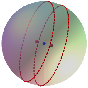
(a) An illustration of the distribution of ${\mathbb{S}}_{0},{\mathbb{S}}_{1}$ on the sphere: the two circles represent the first 1000 vectors in ${\mathbb{S}}_{0},{\mathbb{S}}_{1}$, the red points are their centers. The blue point is the solution, which is also the center of the sphere.

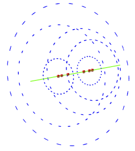
(b) The green line is the set of solutions, the red points are the centers of the blue circles generated by the procedure (6).

Figure 1: Illustrations of Theorems 7 and 12.

Definition 1 (Eigengap inverse).

Let $A$ be an $m\times n$ matrix with no zero rows. Let ${\mathcal{R}}_{A}$ be given in (4). Denote the eigenvalues of ${\mathcal{R}}_{A}$ as $\{e^{i\theta_{1}},\ldots,e^{i\theta_{n}}\}$, where $|\theta_{j}|\leq\pi$. Then we define

$$\eta(A):=\frac{1}{\min_{l:\theta_{l}\neq 0}|\theta_{l}|},$$ (10)

and call it the eigengap inverse of ${\mathcal{R}}_{A}$ (or $A$ for simplicity).

Theorem 9 (restated).

Let $A$ be an $n\times n$ invertible matrix, ${\bf x}_{0},{\bf b}$ be two $n\times 1$ vectors, and ${\bf x}_{*}=A^{-1}{\bf b}$. Let ${\bf y}_{j},{\bf z}_{j}$ be given in (8), (9), then

$$\|\frac{1}{2N}\sum_{i=0}^{N-1}({\bf y}_{i}+{\bf z}_{i})-{\bf x}_{*}\|\leq\varepsilon\|{\bf x}_{0}-{\bf x}_{*}\|,$$ (11)

where

$$N=\left\lceil\frac{\pi\eta(A)}{2\varepsilon}\right\rceil.$$ (12)

Based on the above result, to obtain an approximation of the solution up to relative error $\varepsilon$, we need to generate $O(\eta(A)/\varepsilon)$ points on the sphere. Indeed, this can be reduced to $O(\eta(A)\log(1/\varepsilon))$ by setting $\varepsilon=1/2$ in (11), viewing $\frac{1}{2N}\sum_{i=0}^{N-1}({\bf y}_{i}+{\bf z}_{i})$ as the new approximation of the solution, and restarting the procedure. In this paper, the algorithm for solving linear systems based on (11) will be called the deterministic iterative reflection algorithm. An explicit description of this algorithm is shown in Algorithm 1.

1.1.2 General consistent linear systems

We now turn to the general case. For consistent linear systems, there can be one or infinitely many solutions. In the latter case, the deterministic iterative reflection algorithm demonstrates some interesting properties. The following result states that if we run the deterministic iterative reflection algorithm from ${\bf x}_{0}$, we end up with the solution that has the minimal distance to ${\bf x}_{0}$, see Figure 1(b) for an illustration in dimension 3. In Figure 1(b), each circle is generated by the deterministic iterative reflection algorithm from some ${\bf x}_{0}$. The center of each circle is a solution of the linear system.

Theorem 12 (restated).

Assume that $A{\bf x}={\bf b}$ is consistent. Let ${\bf x}_{0}$ be an arbitrarily chosen initial vector, then $\{{\bf x}_{0},{\bf x}_{1},{\bf x}_{2},\ldots\}$ generated by the process (5) lies on a sphere centered on the solution that has the minimal distance to ${\bf x}_{0}$.

Regarding Theorems 7, 9, we prove that they are also correct if $A$ is reflection consistent (see Definition 18). Reflection consistency is almost equivalent to the claim that $m-r$ is even, where $r$ is the rank of $A$, see Corollary 19. Although the condition that $m-r$ is even is easy to satisfy, it is interesting to see that the algorithm requires this special condition. To satisfy this condition, a simple approach is to randomly introduce some new linear constraints that do not change the solution set of $A{\bf x}={\bf b}$. A difficulty here is that not all linear constraints are allowed. We will show that the set of the new linear constraints such that the deterministic iterative reflection algorithm fails is a set with zero Lebesgue measure. So we can choose almost any linear constraints we want.

Finally, when the linear system $A{\bf x}={\bf b}$ is inconsistent, the deterministic iterative reflection algorithm fails to find the least-squares solution. We show that the deterministic iterative reflection algorithm indeed solves the linear system $A^{{\tt T}}W^{-1}A{\bf x}=A^{{\tt T}}W^{-1}{\bf b}$, where $W$ is the lower-triangular matrix such that $W+W^{{\tt T}}=2AA^{{\tt T}}$. Since solving least-squares problem $\min_{{\bf x}}\|A{\bf x}-{\bf b}\|$ is equivalent to solving $A^{{\tt T}}A{\bf x}=A^{{\tt T}}{\bf b}$, the above finding explains why the deterministic iterative reflection algorithm fails to return the least-squares solution. Note that the new linear system has a similar structure to the generalized least-square problem in statistics [18], where $W$ becomes a covariance matrix. For consistent linear systems, the new linear system $A^{{\tt T}}W^{-1}A{\bf x}=A^{{\tt T}}W^{-1}{\bf b}$ is equivalent to the original one when $A$ is reflection consistent. We will show that under reasonable assumptions, which can be satisfied easily by the idea discussed in the above paragraph for consistent linear systems, the matrix $A^{{\tt T}}W^{-1}A$ is invertible if $A$ has full column-rank. In this case, the new linear system $A^{{\tt T}}W^{-1}A{\bf x}=A^{{\tt T}}W^{-1}{\bf b}$ has a unique solution. Moreover, similar theoretical guarantees to Theorems 7, 9 also hold. Nevertheless, it still remains a problem to modify the deterministic iterative reflection algorithm to solve the least-squares problems.

1.2 Comparison with previous Kaczmarz algorithms

In this part, we theoretically compare the deterministic iterative reflection algorithm with two well-studied randomized Kaczmarz algorithms [41, 28]. The numerical comparisons are given in Section 5.

From Equations (8), (9), we know that ${\bf y}_{i}={\bf x}_{2im}$ and ${\bf z}_{i}={\bf x}_{(2i+1)m}$. Consequently, we can compute ${\bf y}_{i}$ (respectively ${\bf z}_{i}$) from ${\bf y}_{i-1}$ (respectively ${\bf z}_{i-1}$) with $O(mn)$ operations. By Theorem 9, it totally uses $O(mn\eta(A)\log(1/\varepsilon))$ operations to obtain an approximation of the solution up to relative error $\varepsilon$.

Compared to previous Kaczmarz methods [41, 28], it is costly to use $O(mn)$ operations in each step of the iteration. There is actually a simple approach to resolving this problem. We can decompose the set $\mathbb{X}:=\{{\bf x}_{0},{\bf x}_{1},{\bf x}_{2},\ldots\}$ generated by the procedure (5) into a union of $2m$ subsets, which have similar structures to ${\mathbb{S}}_{0},{\mathbb{S}}_{1}$. More precisely, for $k\in\{0,1,\ldots,m-1\}$ and $j\in\{0,1\}$, we define

$${\mathbb{S}}_{kj}:=\{{\bf x}_{*}+{\mathcal{R}}_{k}\cdots{\mathcal{R}}_{1}{\mathcal{R}}_{A}^{2i+j}({\bf x}_{0}-{\bf x}_{*}):i=0,1,2,\ldots\}=\{{\bf x}_{k+(2i+j)m}:i=0,1,2,\ldots\},$$ (13)

then $\mathbb{X}=\cup_{k=0}^{m-1}\cup_{j=0}^{1}{\mathbb{S}}_{kj}$. As a direct consequence, we have similar results to Theorems 7, 9 for each ${\mathbb{S}}_{k0}\cup{\mathbb{S}}_{k1}$. Hence, we can use the average of the first $O(m\eta(A)\log(1/\epsilon))$ points in $\mathbb{X}$ to approximate the solution. This algorithm is summarized in Algorithm 2. It requires more steps of iterations to converge but has a lower computational cost in each step of the iteration. Theoretically, this algorithm has the same complexity as the previous one.

Algorithm	# operations in each step	# iterations	Type
SV [41]	$O(n)$	$O({\kappa_{s}^{2}(A)}\log(1/\varepsilon))$	Randomized
MTMN [28]	$O(n\|A\|_{F}^{2}/\|A\|^{2})$	$O({\kappa^{2}(A)}\log(1/\varepsilon))$	Randomized block
Alg. 1 (This paper)	$O(mn)$	$O({\eta(A)\log(1/\varepsilon)})$	Deterministic
Alg. 2 (This paper)	$O(n)$	$O({m\eta(A)\log(1/\varepsilon)})$	Deterministic

Table 1: Comparison of different Kaczmarz methods, where $\kappa_{s}(A)=\|A\|_{F}\|A^{-1}\|$ is the scaled condition number, $\kappa(A)=\|A\|\|A^{-1}\|$ is the condition number, and $\eta(A)$ is given in Definition 1.

In Table 1, we compare four randomized Kaczmarz algorithms in terms of the number of operations in each step and the total number of iterations.

1. Different from the other two algorithms, Algorithms 1, 2 are influenced by the eigengap inverse $\eta(A)$ arising from the eigenvalues of ${\mathcal{R}}_{A}$. It is generally a quite hard problem to estimate $\eta(A)$. In this paper, we show that $\eta(A)=O((\log n)\kappa^{2}(A))$ in the worst case and $\eta(A)=O(\kappa(A))$ for random matrices when $m\geq n\log n$; see Propositions 10, 11.

2. The overall cost of SV’s and MTMN’s algorithm is $O(n\kappa_{s}^{2}(A)\log(1/\varepsilon))$, and the overall cost of Algorithm 1 is $O(mn\eta(A)\log(1/\varepsilon))$. Note that $\kappa_{s}(A)\leq\min(m,n)\kappa(A)$. So for over-determined linear systems (i.e., $m>n$), Algorithm 1 seems worse even if $\eta(A)=O(\kappa(A))$. This seems reasonable as usually $O(n)$ rows of $A$ are enough to solve over-determined linear systems.

The above theoretical results indicate that Algorithm 1 is usually less efficient in practice. This is not surprising since it uses all the rows of the input matrix when computing a new useful vector. When the linear system is over-determined, this is undesirable. To overcome this problem, in practice, we can modify this algorithm by first computing ${\bf x}_{0},\ldots,{\bf x}_{M-1}$ and then checking the quality of their average as an approximate solution. If it is not a good approximation, then we can restart this process from the average. From our numerical tests in Section 5, this modified algorithm can be faster than SV’s algorithm and can compete with randomized block Kaczmarz algorithms.

1.3 Related work

There are many research papers on the Kaczmarz method, we list below the most related ones. A similar idea was recently used by Steinerberger. In [40], Steinerberger focused on the solving of nonsingular square linear systems using the randomized Kaczmarz method by setting $\alpha_{k}=2$ as well. The randomness is similar to that of Strohmer-Vershynin’s algorithm. Steinerberger proved that

$${\mathbb{E}}\left\|\frac{1}{N}\sum_{j=0}^{N-1}{\bf x}_{j}-A^{-1}{\bf b}\right\|\leq\varepsilon\|{\bf x}_{0}-A^{-1}{\bf b}\|$$ (14)

when $N=O(\kappa_{s}^{2}(A)/\varepsilon^{2})$. So by Markov’s inequality, with high probability the average of the first $N$ vectors can be viewed as an approximation of the solution. Note that in our second algorithm, we have a similar estimate

$$\left\|\frac{1}{N}\sum_{j=0}^{N-1}{\bf x}_{j}-A^{-1}{\bf b}\right\|\leq\varepsilon\|{\bf x}_{0}-A^{-1}{\bf b}\|$$ (15)

when $N=O(n\eta(A)/\varepsilon)$. The ${\bf x}_{j}$’s in (14), (15) have different meanings. Different from Steinerberger’s result, our result is deterministic. In [40], Steinerberger posed an open question of finding a better and deterministic way to approximate the solution from the samples. Our algorithm can be viewed as an answer to this open question – we sample points in a deterministic way and sub-sample smartly so that the samples have predictable structures on the sphere and their average is unbiased with respect to the solution regardless of the linear system used for creating the samples.

Choosing $\alpha_{k}=2$ in (1) is not new. It was highlighted in another famous row projection method proposed by Cimmino in 1938 [9]. In Cimmino’s method, from ${\bf x}_{k}$, we perform $m$ reflections (5) for $i_{k}\in\{1,2,\ldots,m\}$ and use their average to define ${\bf x}_{k+1}$. It was shown by Cimmino that the sequence $\{{\bf x}_{0},{\bf x}_{1},\ldots\}$ converges to a solution under the mild assumption that ${\rm Rank}(A)\geq 2$. In our algorithm, ${\bf x}_{k+1}$ is obtained by one reflection and the sequence $\{{\bf x}_{0},{\bf x}_{1},\ldots\}$ locates on a sphere centered on a solution. The Cimmino method is known to be more amenable to parallelism than the Kaczmarz method. However, the required number of iterations for Cimmino’s method could be large. Compared to Equation (2), the randomized block Kaczmarz method seems to be a generalization of the Cimmino method, except that we are now allowed to set $\alpha_{k}=2$. For more on the connection between the Kaczmarz method and the Cimmino method, we refer to [3, 4].

The idea of using cyclic subsequence $\{{\bf x}_{jm+k}:j=0,1,\ldots,k=0,1,\ldots,m-1\}$ in the Kaczmarz method to solve inconsistent linear systems has been studied decades ago, for example see [42, 7, 14]. In those papers, the authors investigated the problem of using what kind of relaxation parameters the cyclic subsequences will converge to the least-square solution. In [14], Eggermont, Herman, and Lent proved that if the relaxation parameters are periodic, then the cyclic subsequences converge to the least-square solution. It was shown in [7] that when the relaxation parameters tend to zero, the limits of the cyclic subsequences approach the least-square solution.

The original Kaczmarz algorithm [25] is deterministic. There are also some other versions of deterministic Kaczmarz algorithms. We name a few here. For more, we refer to [36, 34, 6, 16] and the references therein. In 1954, Agmon [1], Motzkin and Schoenberg [29] extended the Kaczmarz algorithm to solve linear inequalities by orthogonally projecting the current solution onto the chosen halfspace. In 1957, Hildreth [22] also proposed a similar deterministic algorithm to solve linear inequalities to find the closest point in the solution set to a given point. It is worth mentioning that Hildreth’s algorithm can be reduced to the original Kaczmarz algorithm. In [8], Chen and Huang proposed a deterministic block Kaczmarz method for solving the least-squares problem which is competitive with randomized block Kaczmarz methods. In [35], Nutini et al introduced two greedy selection rules that make the Kaczmarz method deterministic. The greedy selection rules give faster convergence rates, and the costs are similar to the randomized ones in some applications.

1.4 Outline of this paper

In Section 2, we prove some lemmas that will be used in our proofs of the main theorems. In Section 3, we prove our main results for consistent linear systems. In Section 4, we focus on inconsistent linear systems and investigate deeper on the Kaczmarz method. Finally, in Section 5 we compare different Kaczmarz methods numerically.

2 Preliminaries

Throughout this paper, we use $\{{\bf e}_{1},\ldots,{\bf e}_{n}\}$ to denote the standard basis of $\mathbb{R}^{n}$, i.e., for ${\bf e}_{j}$, the $j$-th entry is 1 and all other entries are 0. The $n\times n$ identity matrix will be denoted as $I_{n}$. For the linear system $A{\bf x}={\bf b}$, we always assume that $A$ has no zero rows. All vectors that appear in this paper are assumed to be given in column forms. So when we say the $i$-th row of $A$, we shall use $A_{i}^{{\tt T}}$ because $A_{i}$ refers to a column vector. The operator norm of $A$ is denoted as $\|A\|$. It is the maximal singular value of $A$. With $\|A\|_{F}$, we mean the Frobenius norm, which is the square root of the sum of the absolute squares of the elements of $A$. The condition number refers to the ratio of the largest singular value to the smallest nonzero singular value. For any two vectors ${\bf a},{\bf b}$, their inner product is denoted as $\langle{\bf a}|{\bf b}\rangle$. The transpose of $A$ is denoted as $A^{\tt T}$. We remark again that the notation (3), (4) will be used frequently in this paper.

In this section, we aim to prove some preliminary lemmas that will be used in the next section. The following two lemmas are useful in the proofs of Theorems 7 and 9.

Lemma 2.

Let $\theta_{1},\ldots,\theta_{p}\in(0,2\pi)$ be $p$ distinct parameters and $\{{\bf v}_{1},\ldots,{\bf v}_{p}\}\subseteq\mathbb{R}^{n}$ be a set of orthogonal vectors, then the dimension of the vector space spanned by $\{\sum_{k=1}^{p}(1-e^{ij\theta_{k}}){\bf v}_{k}:j\in\mathbb{N}\}$ is $p$. Moreover, they lie on a sphere centered at $\sum_{k=1}^{p}{\bf v}_{k}$.

Proof.

We consider the following matrix with $p$ columns:

$$M:=\begin{pmatrix}1-e^{i\theta_{1}}&1-e^{2i\theta_{1}}&1-e^{3i\theta_{1}}&\cdots\\ \vdots&\vdots&\vdots&\vdots\\ 1-e^{i\theta_{p}}&1-e^{2i\theta_{p}}&1-e^{3i\theta_{p}}&\cdots\end{pmatrix}.$$

We aim to prove that $M$ is nonsingular.

Since $1-e^{ij\theta_{k}}=(1-e^{i\theta_{k}})(1+e^{i\theta_{k}}+\cdots+e^{i(j-1)\theta_{k}})$ and $e^{i\theta_{k}}\neq 1$, it follows that the rank of $M$ is equal to the rank of the following matrix, which is obtained by dividing the $k$-th row of $M$ with $(1-e^{i\theta_{k}})$:

$$\begin{pmatrix}1&1+e^{i\theta_{1}}&1+e^{i\theta_{1}}+e^{2i\theta_{1}}&\cdots\\ \vdots&\vdots&\vdots&\vdots\\ 1&1+e^{i\theta_{p}}&1+e^{i\theta_{p}}+e^{2i\theta_{p}}&\cdots\end{pmatrix}.$$

Via some column operations, which do not change the rank, the above matrix can be transformed to

$$\begin{pmatrix}1&0&0&\cdots\\ 1&e^{i\theta_{2}}-e^{i\theta_{1}}&e^{2i\theta_{2}}-e^{2i\theta_{1}}&\cdots\\ \vdots&\vdots&\vdots&\vdots\\ 1&e^{i\theta_{p}}-e^{i\theta_{1}}&e^{2i\theta_{p}}-e^{2i\theta_{1}}&\cdots\end{pmatrix}.$$

Now the singularity of $M$ is equivalent to the singularity of the following matrix with $(p-1)$ columns

$$\begin{pmatrix}e^{i\theta_{2}}-e^{i\theta_{1}}&e^{2i\theta_{2}}-e^{2i\theta_{1}}&\cdots\\ \vdots&\vdots&\vdots\\ e^{i\theta_{p}}-e^{i\theta_{1}}&e^{2i\theta_{p}}-e^{2i\theta_{1}}&\cdots\end{pmatrix}.$$

Dividing the $j$-th row with $(e^{i\theta_{j}}-e^{i\theta_{1}})$, which is not zero by assumption, we obtain the following matrix

$$\begin{pmatrix}1&e^{i\theta_{2}}+e^{i\theta_{1}}&e^{2i\theta_{2}}+e^{i\theta_{2}}e^{i\theta_{1}}+e^{2i\theta_{1}}&\cdots\\ \vdots&\vdots&\vdots&\vdots\\ 1&e^{i\theta_{p}}+e^{i\theta_{1}}&e^{2i\theta_{p}}+e^{i\theta_{p}}e^{i\theta_{1}}+e^{2i\theta_{1}}&\cdots\end{pmatrix}\xrightarrow[]{\text{Column operations}}\begin{pmatrix}1&e^{i\theta_{2}}&e^{2i\theta_{2}}&\cdots\\ \vdots&\vdots&\vdots&\vdots\\ 1&e^{i\theta_{p}}&e^{2i\theta_{p}}&\cdots\end{pmatrix}.$$

Finally, the claimed result about the dimension follows directly by induction on $p$. The second claim is straightforward. ∎

The following result is a generalization of Brady-Watt’s formula [5]. Although they only considered the full row-rank case, their result is true generally. Below, we give a simple proof by induction.

Lemma 3 (Brady-Watt’s formula).

Let $A$ be an $m\times n$ matrix with no zero rows, ${\mathcal{R}}_{A}$ be given in (4), then

$${\mathcal{R}}_{A}=I_{n}-2A^{{\tt T}}W^{-1}A,$$

where $W$ is the lower-triangular matrix such that $W+W^{{\tt T}}=2AA^{{\tt T}}$.

Proof.

We prove it by induction on $m$. When $m=1$, the result is clearly true. Now assume that

$${\mathcal{R}}_{A}=I_{n}-2A^{{\tt T}}W_{1}^{-1}A,\quad{\mathcal{R}}_{B}=I_{n}-2B^{{\tt T}}W_{2}^{-1}B,$$

where $W_{1},W_{2}$ are lower-triangular matrices such that $W_{1}+W_{1}^{{\tt T}}=2AA^{{\tt T}}$ and $W_{2}+W_{2}^{{\tt T}}=2BB^{{\tt T}}$. Let $W$ be the lower-triangular matrix such that

$$W+W^{{\tt T}}=2\begin{pmatrix}A\\ B\end{pmatrix}\begin{pmatrix}A^{{\tt T}}&B^{{\tt T}}\end{pmatrix}=\begin{pmatrix}2AA^{{\tt T}}&2AB^{{\tt T}}\\ 2BA^{{\tt T}}&2BB^{{\tt T}}\end{pmatrix}=\begin{pmatrix}W_{1}+W_{1}^{{\tt T}}&2AB^{{\tt T}}\\ 2BA^{{\tt T}}&W_{2}+W_{2}^{{\tt T}}\end{pmatrix}.$$

Namely,

$$W=\begin{pmatrix}W_{1}&0\\ 2BA^{{\tt T}}&W_{2}\end{pmatrix}.$$

It is easy to show that

$$W^{-1}=\begin{pmatrix}W_{1}^{-1}&0\\ -2W_{2}^{-1}BA^{{\tt T}}W_{1}^{-1}&W_{2}^{-1}\end{pmatrix}.$$

Denote $C=\begin{pmatrix}A\\ B\end{pmatrix}$. We then can check that ${\mathcal{R}}_{C}={\mathcal{R}}_{B}{\mathcal{R}}_{A}=I_{n}-2C^{{\tt T}}W^{-1}C$, where $W$ is the lower-triangular matrix such that $W+W^{{\tt T}}=2CC^{{\tt T}}$. Finally, the claimed result follows by induction. ∎

As a corollary of Brady-Watt’s formula, we have the following result. We below present a new proof, which will be helpful in the estimate of the convergence rate in the next section.

Lemma 4.

Assume that $A$ is an $n\times n$ matrix without zero rows, and ${\mathcal{R}}_{A}$ is given in (4), then

$$\det({\mathcal{R}}_{A}-I_{n})=(-2)^{n}\det(A)^{2}\prod_{i=1}^{n}\|A_{i}\|^{-2}.$$

Consequently, 1 is not an eigenvalue of ${\mathcal{R}}_{A}$ if $A$ is nonsingular.

Proof.

From the definition of ${\mathcal{R}}_{A}$, it suffices to consider the case that each row of $A$ has a unit norm. We prove the result by induction on $n$. Assume that $A^{{\tt T}}=QL$ is the QL decomposition of $A^{{\tt T}}$, where $Q$ is orthogonal and $L$ is lower triangular. Then the $i$-th row of $A$, when written in a column vector, equals $A_{i}=QL_{i}$, where $L_{i}$ is the $i$-th column of $L$. As a result, we have

$${\mathcal{R}}_{A}=Q\prod_{i=1}^{n}(I_{n}-2L_{i}L_{i}^{{\tt T}})Q^{{\tt T}}.$$

The eigenvalues and the determinant of ${\mathcal{R}}_{A}$ are the same as those of $\prod_{i=1}^{n}(I-2L_{i}L_{i}^{{\tt T}})$. Hence, without loss of generality, we can assume that $A$ is a lower triangular matrix satisfying that each row has a unit norm.

When $n=1$, we have $A=1$ and ${\mathcal{R}}_{A}=-1$. Thus, $\det({\mathcal{R}}_{A}-I_{1})=-2$. When $n=2$, $A=\begin{pmatrix}1&0\\ a&b\\ \end{pmatrix}$ where $a^{2}+b^{2}=1$. Thus ${\mathcal{R}}_{A}=\begin{pmatrix}2a^{2}-1&-2ab\\ 2ab&1-2b^{2}\\ \end{pmatrix}$. We now can directly check that $\det({\mathcal{R}}_{A}-I_{2})=4b^{2}$. When $n\geq 3$, we denote the last row of $A$ as $({\bf v}^{{\tt T}},w)$, where ${\bf v}\in\mathbb{R}^{n-1}$ is a column vector and $w\in\mathbb{R}^{*}$. For convenience, we denote the submatrix with the last row and column of $A$ removed as $B$. Then it is easy to show that

$${\mathcal{R}}_{A}=\begin{pmatrix}(I_{n-1}-2{\bf v}{\bf v}^{{\tt T}}){\mathcal{R}}_{B}&-2w{\bf v}\\ -2w{\bf v}^{{\tt T}}{\mathcal{R}}_{B}&1-2w^{2}\\ \end{pmatrix}.$$

Therefore,

$${\mathcal{R}}_{A}-I_{n} = \begin{pmatrix}(I_{n-1}-2{\bf v}{\bf v}^{{\tt T}}){\mathcal{R}}_{B}-I_{n-1}&-2w{\bf v}\\ -2w{\bf v}^{{\tt T}}{\mathcal{R}}_{B}&-2w^{2}\\ \end{pmatrix}$$

$$= \begin{pmatrix}I_{n-1}&0\\ 0&w\\ \end{pmatrix}\begin{pmatrix}(I_{n-1}-2{\bf v}{\bf v}^{{\tt T}}){\mathcal{R}}_{B}-I_{n-1}&{\bf v}\\ -2{\bf v}^{{\tt T}}{\mathcal{R}}_{B}&1\\ \end{pmatrix}\begin{pmatrix}I_{n-1}&0\\ 0&-2w\\ \end{pmatrix}.$$

It implies

$$\det({\mathcal{R}}_{A}-I_{n})=-2w^{2}\det\begin{pmatrix}(I_{n-1}-2{\bf v}{\bf v}^{{\tt T}}){\mathcal{R}}_{B}-I_{n-1}&{\bf v}\\ -2{\bf v}^{{\tt T}}{\mathcal{R}}_{B}&1\\ \end{pmatrix}=-2w^{2}\det({\mathcal{R}}_{B}-I_{n-1}).$$

By induction, we have $\det({\mathcal{R}}_{A}-I_{n})=(-2)^{n}\det(A)^{2}$. ∎

The next lemma will be used to estimate an upper bound of $\eta(A)$ in terms of the condition number of $A$. The triangular truncation operator $T$ is defined as an $m\times m$ matrix such that $T_{ij}=1$ if $i\geq j$ and 0 otherwise. Denote

$$K_{m}:=\max\left\{\frac{\|A\circ T\|}{\|A\|}:A\text{ is }m\times m\text{ and nonzero},\circ\text{ is the Hadamard product}\right\}.$$

Lemma 5 (Theorem 1 of [2]).

For $m\geq 2$,

$$\left|\frac{K_{m}}{\log m}-\frac{1}{\pi}\right|\leq\left(1+\frac{1}{\pi}\right)\frac{1}{\log m}.$$

The above result suggests that $\|A\circ T\|=O(\|A\|\log m)$ for any $m\times m$ matrix $A$.

3 Consistent linear systems

We now turn our attention to the main results of solving linear systems $A{\bf x}={\bf b}$ by the Kaczmarz method. First, we explicitly describe our main algorithm for solving consistent linear systems in Algorithm 1 below. Then, we analyze its correctness and efficiency. To better understand the geometric structures of the algorithm, we first focus on the case that $A$ is invertible. We then extend the results to general consistent linear systems. In this section, the notation (3), (4), (8), (9) will be widely used.

Algorithm 1 Deterministic iterative reflection algorithm for solving consistent linear systems

1:A consistent linear system $A{\bf x}={\bf b}$, an arbitrarily chosen initial vector ${\bf x}_{0}$ and an accuracy $\varepsilon\in[0,1]$.

2:Output $\tilde{{\bf x}}$ such that $\|A\tilde{{\bf x}}-{\bf b}\|\leq\varepsilon$.

3:For $k=0,1,2,\cdots$, compute

$${\bf x}_{k+1}={\bf x}_{k}+2\frac{b_{i_{k}}-A_{i_{k}}^{{\tt T}}{\bf x}_{k}}{\|A_{i_{k}}\|^{2}}A_{i_{k}},$$ (16)

where $i_{k}=(k\mod m)+1$.

4:Stop the iteration at step $m(M-1)$ if $\|A\tilde{{\bf x}}-{\bf b}\|\leq\varepsilon$, where $\tilde{{\bf x}}=\frac{1}{M}\sum_{j=0}^{M-1}{\bf x}_{jm}$.

5:Output $\tilde{{\bf x}}$.

Remark 6.

Before presenting all the results, we want to emphasize in a less rigorous way that Algorithm 1 only works for consistent linear systems under the mild assumption that $m-r$ is even, where $r$ is the rank of $A$.

3.1 Case 1: $A$ is invertible

When $A$ is invertible, the solution is unique. This greatly simplifies the analysis of Algorithm 1. The geometric feature of the algorithm is also very clear in this case. Moreover, this case is a theoretical building block for the general case.

Note that $m=n$ in this case. As discussed in the introduction (see (13)), in (8), (9), we know that ${\mathbb{S}}_{0},{\mathbb{S}}_{1}$ are only two subsets of $\mathbb{X}=\{{\bf x}_{l}:l=0,1,2,\ldots\}$. We can decompose $\mathbb{X}$ into a union of $2n$ subsets, which have similar structures to ${\mathbb{S}}_{0},{\mathbb{S}}_{1}$. More precisely, for $k=0,1,\ldots,n-1$ and $j=0,1$, define

$${\mathbb{S}}_{kj} := \{{\bf x}_{*}+{\mathcal{R}}_{k}\cdots{\mathcal{R}}_{1}{\mathcal{R}}^{2i+j}({\bf x}_{0}-{\bf x}_{*}):i=0,1,2,\ldots\}$$ (17)

$$= \{{\bf x}_{*}+({\mathcal{R}}_{k}\cdots{\mathcal{R}}_{1}{\mathcal{R}}_{n}\cdots{\mathcal{R}}_{k+1})^{2i+j}({\bf x}_{k}-{\bf x}_{*}):i=0,1,2,\ldots\}$$ (18)

$$= \{{\bf x}_{k+(2i+j)n}:i=0,1,2,\ldots\},$$ (19)

where ${\bf x}_{k}={\bf x}_{*}+{\mathcal{R}}_{k}\cdots{\mathcal{R}}_{1}({\bf x}_{0}-{\bf x}_{*})$. Hence we have $\mathbb{X}=\cup_{k=0}^{n-1}\cup_{j=0}^{1}{\mathbb{S}}_{kj}$. This decomposition is a theoretical guarantee of our second algorithm below. Using this notation, ${\mathbb{S}}_{0j}={\mathbb{S}}_{j}$ for $j=0,1$. Recall that the sphere with minimal dimension such that ${\mathbb{S}}_{j}$ lies on it is called the minimal sphere supporting ${\mathbb{S}}_{j}$.

Theorem 7.

For $j=0,1$, let ${\bf c}_{j}$ be the center of the minimal sphere supporting ${\mathbb{S}}_{j}$, then ${\bf c}_{0}+{\bf c}_{1}=2{\bf x}_{*}$.

Proof.

Let ${\mathcal{R}}_{A}=U^{\dagger}DU$ be the eigenvalue decomposition of ${\mathcal{R}}_{A}$, where $U$ is unitary, $D$ is diagonal, and “ ${\dagger}$ ” refers to the conjugate transpose operator. For convenience, we assume that ${\bf x}_{0}=0$. If ${\bf x}_{0}\neq 0$, we can consider ${\bf x}_{0}-{\bf y}_{j},{\bf x}_{0}-{\bf z}_{j}$ instead. This is just a translation, which will not affect the final result. With the above notation, we have ${\bf y}_{j}=U^{\dagger}(I-D^{2j})U{\bf x}_{*}$ and ${\bf z}_{j}=U^{\dagger}(I-D^{2j+1})U{\bf x}_{*}$.

Denote $\tilde{{\bf y}}_{j}=U{\bf y}_{j},\tilde{{\bf z}}_{j}=U{\bf z}_{j},\tilde{{\bf x}}_{*}=U{\bf x}_{*}=\sum_{k=1}^{n}x_{k}{\bf e}_{k}$, and $D={\rm diag}(e^{i\theta_{1}},\ldots,e^{i\theta_{n}})$, where $|\theta_{i}|\leq\pi$ for all $i$. Then

$$\tilde{{\bf y}}_{j}=\sum_{k=1}^{n}(1-e^{2ij\theta_{k}})x_{k}{\bf e}_{k},\quad\tilde{{\bf z}}_{j}=\sum_{k=1}^{n}(1-e^{i(2j+1)\theta_{k}})x_{k}{\bf e}_{k}.$$

For convenience, we denote all the distinct eigen-phases $\{\theta_{1},\ldots,\theta_{n}\}$ of ${\mathcal{R}}_{A}$ as $\{\phi_{1},\phi_{2},\pm\phi_{3},\ldots,\pm\phi_{L}\}$, where $\phi_{1}=\pi,\phi_{2}=0$ and $0<\phi_{l}<\pi$ for $3\leq l\leq L$. Certainly, it may happen that $\pi,0\not\in\{\theta_{1},\ldots,\theta_{n}\}$. However, this will not influence the following analysis.

We first determine the center of the minimal sphere supporting ${\mathbb{S}}_{0}$. Note that

$$\tilde{{\bf y}}_{j} = \sum_{k=1}^{L}(1-e^{2ij\phi_{k}})\sum_{l:\theta_{l}=\phi_{k}}x_{l}{\bf e}_{l}+\sum_{k=1}^{L}(1-e^{-2ij\phi_{k}})\sum_{l:\theta_{l}=-\phi_{k}}x_{l}{\bf e}_{l}$$

$$= \sum_{k=3}^{L}\left(1-e^{ij(2\phi_{k})}\right)\sum_{l:\theta_{l}=\phi_{k}}x_{l}{\bf e}_{l}+\sum_{k=3}^{L}\left(1-e^{ij(2(\pi-\phi_{k}))}\right)\sum_{l:\theta_{l}=-\phi_{k}}x_{l}{\bf e}_{l}.$$

Without loss of generality, we assume that $\sum_{l:\theta_{l}=\phi_{k}}x_{l}{\bf e}_{l}\neq 0,\sum_{l:\theta_{l}=-\phi_{k}}x_{l}{\bf e}_{l}\neq 0$ for all $k\geq 3$, otherwise we just ignore them. Since $0<2\phi_{k},2(\pi-\phi_{k})<2\pi$, it then follows from Lemma 2 that the dimension of the vector space spanned by $\{\tilde{{\bf y}}_{j}:j=0,1,2,\ldots\}$ is $2L-4$. Moreover, the center of the minimal sphere that supports this vector space is

$$\sum_{k=3}^{L}~{}\sum_{l:\theta_{l}=\phi_{k}}x_{l}{\bf e}_{l}+\sum_{k=3}^{L}~{}\sum_{l:\theta_{l}=-\phi_{k}}x_{l}{\bf e}_{l}=\tilde{{\bf x}}_{*}-\sum_{l:\theta_{l}=\pi}x_{l}{\bf e}_{l}-\sum_{l:\theta_{l}=0}x_{l}{\bf e}_{l}.$$ (20)

Regarding the center of the minimal sphere supporting ${\mathbb{S}}_{1}$, we notice that

$$\tilde{{\bf z}}_{j}=\sum_{k=1}^{n}(1-e^{i\theta_{k}})x_{k}{\bf e}_{k}+\sum_{k=1}^{n}(1-e^{2ij\theta_{k}})e^{i\theta_{k}}x_{k}{\bf e}_{k}.$$

The first term is a translation and the second term can be analyzed in a similar way to $\tilde{{\bf y}}_{j}$. Thus the dimension of the vector space spanned by ${\mathbb{S}}_{1}$ is also $2L-4$, and the center of the minimal sphere that supports $\{\tilde{{\bf z}}_{j}:j=0,1,2,\ldots\}$ is

$$\sum_{k=1}^{n}(1-e^{i\theta_{k}})x_{k}{\bf e}_{k}+\sum_{k=1}^{n}e^{i\theta_{k}}x_{k}{\bf e}_{k}-\sum_{l:\theta_{l}=\pi}e^{i\theta_{l}}x_{l}{\bf e}_{l}-\sum_{l:\theta_{l}=0}e^{i\theta_{l}}x_{l}{\bf e}_{l}$$ (21)

$$= \tilde{{\bf x}}_{*}+\sum_{l:\theta_{l}=\pi}x_{l}{\bf e}_{l}-\sum_{l:\theta_{l}=0}x_{l}{\bf e}_{l}.$$

By Lemma 4, $\theta_{l}\neq 0$ for all $l$. Namely, the third term in (20), (21) does not exist. Therefore, we have

$${\bf c}_{0}=U^{\dagger}\Big{(}\tilde{{\bf x}}_{*}-\sum_{l:\theta_{l}=\pi}x_{l}{\bf e}_{l}\Big{)},\quad{\bf c}_{1}=U^{\dagger}\Big{(}\tilde{{\bf x}}_{*}+\sum_{l:\theta_{l}=\pi}x_{l}{\bf e}_{l}\Big{)}.$$

This implies ${\bf c}_{0}+{\bf c}_{1}=2{\bf x}_{*}$. ∎

As a corollary, we can compute the center of the minimal sphere that supports ${\mathbb{S}}_{kj}$ for any $k,j$. More precisely, we have the following result.

Corollary 8.

Assume that the unit eigenvectors of ${\mathcal{R}}_{A}$ corresponding to $-1$ are ${\bf u}_{1},\ldots,{\bf u}_{q}$, then the center of the minimal sphere supporting ${\mathbb{S}}_{kj}$ is ${\bf c}_{kj}=(I_{n}-{\mathcal{R}}_{k}\cdots{\mathcal{R}}_{1}){\bf x}_{*}+{\mathcal{R}}_{k}\cdots{\mathcal{R}}_{1}{\bf c}_{j},$ where

$${\bf c}_{j}={\bf x}_{0}+\Big{(}I_{n}-(-1)^{j}\sum_{l=1}^{q}{\bf u}_{l}{\bf u}_{l}^{{\tt T}}\Big{)}({\bf x}_{*}-{\bf x}_{0}),\quad j\in\{0,1\}.$$

Consequently, ${\bf c}_{k0}+{\bf c}_{k1}=2{\bf x}_{*}$ for all $k=0,1,\ldots,n-1$.

Proof.

As we can see from the proof of Theorem 7, when ${\bf x}_{0}=0$ the centers of ${\mathbb{S}}_{0},{\mathbb{S}}_{1}$ are respectively

$${\bf c}_{0}=\Big{(}I_{n}-\sum_{l=1}^{q}{\bf u}_{l}{\bf u}_{l}^{{\tt T}}\Big{)}{\bf x}_{*},\quad{\bf c}_{1}=\Big{(}I_{n}+\sum_{l=1}^{q}{\bf u}_{l}{\bf u}_{l}^{{\tt T}}\Big{)}{\bf x}_{*}.$$

To understand the center of ${\mathbb{S}}_{kj}$, we first respectively compute the centers of the minimal spheres supporting ${\mathbb{S}}_{0},{\mathbb{S}}_{1}$ for ${\bf x}_{0}\neq 0$. When ${\bf x}_{0}\neq 0$, we have

$${\bf y}_{i}={\bf x}_{*}+{\mathcal{R}}_{A}^{2i}({\bf x}_{0}-{\bf x}_{*})={\bf x}_{0}+(I_{n}-{\mathcal{R}}_{A}^{2i})({\bf x}_{*}-{\bf x}_{0}),$$

so we can focus on $\{{\bf y}_{i}-{\bf x}_{0}:i=0,1,2,\ldots\}={\mathbb{S}}_{0}-{\bf x}_{0}$ in the proof of Theorem 7, which is a translation of ${\mathbb{S}}_{0}$. Similar to the proof of Theorem 7, we have

$${\bf c}_{0}={\bf x}_{0}+\Big{(}I_{n}-\sum_{l=1}^{q}{\bf u}_{l}{\bf u}_{l}^{{\tt T}}\Big{)}({\bf x}_{*}-{\bf x}_{0}),\quad{\bf c}_{1}={\bf x}_{0}+\Big{(}I_{n}+\sum_{l=1}^{q}{\bf u}_{l}{\bf u}_{l}^{{\tt T}}\Big{)}({\bf x}_{*}-{\bf x}_{0}).$$

We next compute the center of the minimal sphere supporting ${\mathbb{S}}_{kj}$. From the above analysis and note that the vectors in ${\mathbb{S}}_{kj}$ have the form ${\bf x}_{k}+(I_{n}-({\mathcal{R}}_{k}\cdots{\mathcal{R}}_{1}{\mathcal{R}}_{n}\cdots{\mathcal{R}}_{k+1})^{2i+j})({\bf x}_{*}-{\bf x}_{k})$ by (18), we have that the center of the minimal sphere supporting ${\mathbb{S}}_{kj}$ equals

$${\bf c}_{kj}={\bf x}_{k}+\Big{(}I_{n}-(-1)^{j}\sum_{l=1}^{q}{\bf u}_{kl}{\bf u}_{kl}^{{\tt T}}\Big{)}({\bf x}_{*}-{\bf x}_{k}),$$

where ${\bf u}_{kl}$ are the unit eigenvectors of ${\mathcal{R}}_{k}\cdots{\mathcal{R}}_{1}{\mathcal{R}}_{n}\cdots{\mathcal{R}}_{k+1}$ corresponding to the eigenvalue $-1$. Since

$${\mathcal{R}}_{k}\cdots{\mathcal{R}}_{1}{\mathcal{R}}_{n}\cdots{\mathcal{R}}_{k+1}=({\mathcal{R}}_{k}\cdots{\mathcal{R}}_{1}){\mathcal{R}}_{A}({\mathcal{R}}_{k}\cdots{\mathcal{R}}_{1})^{{\tt T}},$$

it follows that ${\bf u}_{kl}={\mathcal{R}}_{k}\cdots{\mathcal{R}}_{1}{\bf u}_{l}$. Also note that ${\bf x}_{k}=(I_{n}-{\mathcal{R}}_{k}\cdots{\mathcal{R}}_{1}){\bf x}_{*}+{\mathcal{R}}_{k}\cdots{\mathcal{R}}_{1}{\bf x}_{0}$, so we can rewrite the center as

$${\bf c}_{kj} = (I_{n}-{\mathcal{R}}_{k}\cdots{\mathcal{R}}_{1}){\bf x}_{*}+{\mathcal{R}}_{k}\cdots{\mathcal{R}}_{1}{\bf x}_{0}+{\mathcal{R}}_{k}\cdots{\mathcal{R}}_{1}\Big{(}I_{n}-(-1)^{j}\sum_{l=1}^{q}{\bf u}_{l}{\bf u}_{l}^{{\tt T}}\Big{)}({\bf x}_{*}-{\bf x}_{0})$$

$$= (I_{n}-{\mathcal{R}}_{k}\cdots{\mathcal{R}}_{1}){\bf x}_{*}+{\mathcal{R}}_{k}\cdots{\mathcal{R}}_{1}{\bf c}_{j}.$$

This completes the proof. ∎

From Corollary 8, we see that if $n$ is odd, then $q\geq 1$ and so ${\bf c}_{0}\neq{\bf c}_{1}\neq{\bf x}_{*}$ unless ${\bf x}_{*}$ has no overlap in the eigenspace of ${\mathcal{R}}_{A}$ corresponding to the eigenvalue $-1$. However, if $n$ is even, it may happen that $q=0$. In this case ${\bf c}_{0}={\bf c}_{1}={\bf x}_{*}$. When this happens, ${\mathbb{S}}_{0},{\mathbb{S}}_{1}$ are on the same minimal sphere.

Theorem 7 implies the correctness of Algorithm 1. Next, we consider its efficiency.

Theorem 9.

Let $A$ be an $n\times n$ invertible matrix, ${\bf x}_{0},{\bf b}$ be two $n\times 1$ vectors, and ${\bf x}_{*}=A^{-1}{\bf b}$. Let ${\bf y}_{j},{\bf z}_{j}$ be given in (8), (9), then

$$\|\frac{1}{2N}\sum_{j=0}^{N-1}({\bf y}_{j}+{\bf z}_{j})-{\bf x}_{*}\|\leq\varepsilon\|{\bf x}_{0}-{\bf x}_{*}\|,$$ (22)

where

$$N=\left\lceil\frac{\pi\eta(A)}{2\varepsilon}\right\rceil$$ (23)

and $\eta(A)$ is given in Definition 1.

Proof.

Denote

$$\tilde{{\bf x}}=\frac{1}{2N}\sum_{j=0}^{N-1}({\bf y}_{j}+{\bf z}_{j}).$$

From the construction of ${\bf y}_{j},{\bf z}_{j}$, we have

$$\tilde{{\bf x}}=\frac{1}{2N}\sum_{j=0}^{2N-1}\Big{(}{\bf x}_{*}+{\mathcal{R}}_{A}^{j}({\bf x}_{0}-{\bf x}_{*})\Big{)}={\bf x}_{*}+\frac{1}{2N}\sum_{j=0}^{2N-1}{\mathcal{R}}_{A}^{j}({\bf x}_{0}-{\bf x}_{*}).$$

Assume that the unit eigenvectors of ${\mathcal{R}}_{A}$ are ${\bf u}_{l},l\in\{1,\ldots,n\}$. We decompose ${\bf x}_{0}-{\bf x}_{*}=\sum_{l=1}^{n}\beta_{l}{\bf u}_{l}$, then by the orthogonality of $\{{\bf u}_{l}\}_{l=1}^{n}$, it is easy to show that

$$\|\tilde{{\bf x}}-{\bf x}_{*}\|^{2} = \frac{1}{4N^{2}}\left\|\sum_{j=0}^{2N-1}{\mathcal{R}}_{A}^{j}({\bf x}_{0}-{\bf x}_{*})\right\|^{2}$$

$$= \frac{1}{4N^{2}}\left\|\sum_{l=1}^{n}\beta_{l}\left(\sum_{j=0}^{2N-1}e^{ij\theta_{l}}\right){\bf u}_{l}\right\|^{2}$$

$$= \frac{1}{4N^{2}}\sum_{l=1}^{n}|\beta_{l}|^{2}\left|\sum_{j=0}^{2N-1}e^{ij\theta_{l}}\right|^{2}$$

$$= \frac{1}{4N^{2}}\sum_{l=1}^{n}|\beta_{l}|^{2}\left|\frac{1-e^{2iN\theta_{l}}}{1-e^{i\theta_{l}}}\right|^{2}$$

$$= \frac{1}{4N^{2}}\sum_{l=1}^{n}|\beta_{l}|^{2}\frac{\sin^{2}(N\theta_{l})}{\sin^{2}(\theta_{l}/2)}.$$

Notice that if $0<|\theta_{l}|\leq\pi$, we have $|\sin(\theta_{l}/2)|\geq|\theta_{l}|/\pi$. This means that ${\sin^{2}(N\theta_{l})}/{\sin^{2}(\theta_{l}/2)}\leq\pi^{2}/\theta_{l}^{2}$. By Lemma 4, $\theta_{l}\neq 0$ for all $l$. Hence,

$$\|\tilde{{\bf x}}-{\bf x}_{*}\|^{2}\leq\frac{\pi^{2}\|{\bf x}_{0}-{\bf x}_{*}\|^{2}}{4N^{2}\min_{l}|\theta_{l}|^{2}}.$$

Set the above estimate as $\varepsilon^{2}\|{\bf x}_{0}-{\bf x}_{*}\|^{2}$, we then have

$$N=\left\lceil\frac{\pi}{2\varepsilon\min_{l}|\theta_{l}|}\right\rceil=\left\lceil\frac{\pi\eta(A)}{2\varepsilon}\right\rceil.$$

This completes the proof. ∎

As already mentioned in the introduction, based on the above result, to obtain an approximation of the solution up to relative error $\varepsilon$, we can modify Algorithm 1 by only using $O(\eta(A)\log(1/\varepsilon))$ iterations. The basic idea is as follows: In Equation (22), we choose $\varepsilon=1/2$, then $N=\lceil\pi\eta(A)\rceil$ and $\|\tilde{{\bf x}}_{0}-{\bf x}_{*}\|\leq 0.5\|{\bf x}_{0}-{\bf x}_{*}\|,$ where $\tilde{{\bf x}}_{0}=\frac{1}{2N}\sum_{j=0}^{N-1}({\bf y}_{j}+{\bf z}_{j})$. We now view $\tilde{{\bf x}}_{0}$ as the new initial vector and repeat the above procedure. After $\log(1/\varepsilon)$ iterations, we obtain an approximation of the solution up to relative error $\varepsilon$. The total number of iterations is $O(\eta(A)\log(1/\varepsilon))$.

In Algorithm 1, we only focused on ${\bf x}_{jm}$ for $j\in\{0,1,\ldots,M-1\}$. So it costs $O(mn)$ to compute ${\bf x}_{(j+1)m}$ from ${\bf x}_{jm}$. Previous Kaczmarz algorithms usually use $O(n)$ operations at each step of the iteration. We can solve this problem by proposing the following algorithm, the correctness of which is guaranteed by Corollary 8 and Theorem 9.

Algorithm 2 The second deterministic iterative reflection algorithm

1:A consistent linear system $A{\bf x}={\bf b}$, an arbitrarily chosen initial vector ${\bf x}_{0}$, and $\varepsilon\in[0,1]$.

2:Output $\tilde{{\bf x}}$ such that $\|A\tilde{{\bf x}}-{\bf b}\|\leq\varepsilon$.

3:For $k=0,1,2,\cdots$, compute

$${\bf x}_{k+1}={\bf x}_{k}+2\frac{b_{i_{k}}-A_{i_{k}}^{{\tt T}}{\bf x}_{k}}{\|A_{i_{k}}\|^{2}}A_{i_{k}},$$ (24)

where $i_{k}=(k\mod m)+1$.

4:Stop the iteration at step $N$ if $\|A\tilde{{\bf x}}-{\bf b}\|\leq\varepsilon$, where $\tilde{{\bf x}}=\frac{1}{N}\sum_{j=0}^{N-1}{\bf x}_{j}$.

5:Output $\tilde{{\bf x}}$.

Compared with Algorithm 1, this algorithm is easier to implement because it only uses $O(n)$ operations at each step of the iteration. But it requires more steps to converge. The overall complexity of these two algorithms is the same in theory. To run Algorithm 2 in practice, we can use a similar idea introduced above to reduce the dependence on $\varepsilon$ to $\log(1/\varepsilon)$. That is we compute some $\tilde{{\bf x}}$ and restart the iteration from $\tilde{{\bf x}}$ if it is not a good approximation of the solution. It turns out that this is very efficient in practice, see the numerical results in Section 5.

The convergence rates of the algorithms proposed in this paper highly depend on $\eta(A)$. To obtain a better understanding, at the end of this section, we build its connection to the condition number of $A$. Theoretically, we have the following general upper bound.

Proposition 10.

Let $A$ be an $m\times n$ matrix, then $\eta(A)=O((\log m)\kappa^{2}(A))$.

Proof.

By Lemma 3, we have ${\mathcal{R}}_{A}=I_{n}-2A^{{\tt T}}W^{-1}A$, where $W$ is the lower-triangular matrix such that $W+W^{{\tt T}}=2AA^{{\tt T}}$. Now assume that $e^{i\theta}$ is the eigenvalue of ${\mathcal{R}}_{A}$ such that $\theta$ is minimal and nonzero. Set the corresponding unit eigenvector as ${\bf u}$, then we have $|1-e^{i\theta}|=2\|A^{{\tt T}}W^{-1}A{\bf u}\|$. We consider the case that $\theta>0$ is close to 0 so that the left-hand side is as small as $\theta$. The right-hand side is lower bounded by $2\sigma_{\min}(A)^{2}\sigma_{\min}(W^{-1})$, where $\sigma_{\min}$ refers to the minimal nonzero singular value. Thus $1/\theta=O(\|W\|/\sigma_{\min}(A)^{2})$. Since $W+W^{{\tt T}}=2AA^{{\tt T}}$, we know that $W=(2AA^{{\tt T}})\circ T-{\rm diag}(\|A_{1}^{{\tt T}}\|,\cdots,\|A_{m}^{{\tt T}}\|)$, where $T$ is the triangular truncation operator defined above Lemma 5. By Lemma 5, we have

$$\|W\|\leq\frac{\log m}{\pi}\|2AA^{{\tt T}}\|+\max_{1\leq i\leq m}\|A_{i}^{{\tt T}}\|\leq\frac{2\log m}{\pi}\|A\|^{2}+\|A\|.$$

Therefore, we have $1/\theta=O((\log m)\kappa^{2}(A))$. ∎

The upper bound in the above proposition can be reached in some cases. For example, consider the case $m=n=3$. For simplicity, we assume that

$$A=\begin{pmatrix}1&0&0\\ \cos(x)&\sin(x)&0\\ \cos^{2}(x)&\cos(x)\sin(x)&\sin(x)\\ \end{pmatrix},$$

where $\sin(x)\neq 0$. Then direct calculation shows that the singular values of $A$ are

$$|\sin(x)|,\quad\sqrt{\frac{1}{2}\left(2+\cos^{2}(x)\pm|\cos(x)|\sqrt{8+\cos^{2}(x)}\right)}.$$

Let $x$ tend to 0, then the singular values are approximately equal to $|x|,3,|x|/3.$ Thus the condition number is $\kappa(A)=\Theta(1/|x|)$. We can also compute that the eigenvalues of ${\mathcal{R}}_{A}$ are

$$-1,\,\,\,1-2\sin^{4}(x)\pm 2i\sin^{2}(x)\sqrt{1-\sin^{4}(x)}.$$

When $x$ is close to 0, the eigenvalues are close to $-1,1\pm 2ix^{2}$, which means $\min|\theta_{l}|\approx x^{2}\approx 1/\kappa^{2}(A)$. Note that when $x\approx 0$, the rows of $A$ are close to each other and ${\mathcal{R}}_{A}$ is close to ${\rm diag}\{-1,1,1\}$. In the high-dimensional case, as suggested by the numerical tests, for matrices with the same structure as $A$ (i.e., the $i$-th row is the polar coordinate of a unit vector, all rows use the same parameter $x$), we always have $\min|\theta_{l}|\approx 1/\kappa^{2}$ when $x\approx 0$.

Below we show that for random matrices, $\eta(A)\approx\kappa(A)$. Let $U$ be a random orthogonal matrix taken from the orthogonal group of dimension $n$ uniformly according to the Haar measure. Denote the eigenvalues of $U$ by $\{e^{i\theta_{1}},\ldots,e^{i\theta_{n}}\}$. For any $\theta\geq 0$, denote $\mathcal{N}_{\theta}=\#\{j:0\leq\theta_{j}\leq\theta\}$. Then according to random matrix theory [27, Proposition 4.7], we have

$$\left|{\mathbb{E}}[\mathcal{N}_{\theta}]-\frac{n\theta}{\pi}\right|\leq\frac{1+\pi}{2\pi}.$$ (25)

If we choose $\theta=1/10n$, then ${\mathbb{E}}[\mathcal{N}_{\theta}]\leq(1+\pi)/2\pi+1/10\pi<0.7$. By Markov’s inequality

$${\rm Prob}[\mathcal{N}_{\theta}>1]\leq{\mathbb{E}}[\mathcal{N}_{\theta}]<0.7.$$

Thus $\mathcal{N}_{\theta}=0$ with probability at least 0.3. Equivalently, with probability at least 0.3, we have $\min|\theta|\geq 1/10n$.

If we pick a point ${\bf v}$ uniformly random on the unit sphere of dimension $n$, then $I_{n}-2{\bf v}{\bf v}^{T}$ defines a reflection in the hyperplane orthogonal to ${\bf v}$. We obtain a random orthogonal matrix by forming a product of independent copies of these reflections. The question is how many random reflections are required to get close to the Haar measure. In [10, page 187], it was shown that $0.5n\log n+\alpha n$ random reflections are required, where $\alpha$ is a universal constant independent of $n$. So ${\mathcal{R}}_{A}$ is a random orthogonal matrix under the Haar measure when $m=\Omega(n\log n)$. In this case, from the above analysis, $\eta(A)<10n$ with probability at least 0.3, and $\eta(A)\approx n/\pi\approx 0.32n$ on average from (25). In summary, we have the following result.

Proposition 11.

Let $A$ be an $m\times n$ random matrix whose rows are uniformly random vectors. Assume that $m=\Omega(n\log n)$. Then $\eta(A)\approx n/\pi$ on average and $\eta(A)<10n$ with probability at least 0.3.

Assume that $A$ is $n\times n$ and that all the entries independently follow the standard normal distribution. Then it was shown in [13, Theorem 7.1] that ${\mathbb{E}}[\log\kappa(A)]=\log n+c+o(1)$ when $n$ is sufficiently large, where $c\approx 1.537$. So on average, $\kappa(A)\approx e^{1.537}n\approx 4.65n$. It follows from Corollary 7.1 of [13] that ${\rm Prob}[\kappa(A)<xn]=e^{-2/x-2/x^{2}}.$ For example, if we choose $x=10$, then $\kappa(A)<10n$ with probability close to 0.8. Therefore, for random Gaussian matrices, on average $\eta(A)\approx\kappa(A)\approx n.$ This result is better than Proposition 10.

3.2 Case 2: $A$ has full row-rank

We now turn to the general case. Assume that $A$ is $m\times n$. We first focus on the case that $A$ has full row-rank $m$. Then we extend our ideas to general consistent linear systems.

For consistent linear systems with $m<n$, there are an infinite number of solutions. Although the situation looks complicated now, we will see that some interesting properties will appear. The definitions of ${\mathcal{R}}_{i},{\mathcal{R}}_{A}$ are the same as those in (3), (4). As for ${\mathbb{S}}_{0},{\mathbb{S}}_{1}$, the change is slight. Compared to (8), (9), they now become ${\mathbb{S}}_{0}=\{{\bf x}_{0},{\bf x}_{2m},{\bf x}_{4m},\ldots\},{\mathbb{S}}_{1}=\{{\bf x}_{m},{\bf x}_{3m},{\bf x}_{5m},\ldots\}.$ Below, $\{{\bf x}_{0},{\bf x}_{1},\ldots\}$ still refers to the series of vectors generated by the procedure (24).

The following result holds for all consistent linear systems.

Theorem 12.

Assume that $A{\bf x}={\bf b}$ is consistent. Let ${\bf x}_{0}$ be an arbitrarily chosen initial vector, then $\{{\bf x}_{0},{\bf x}_{1},{\bf x}_{2},\ldots\}$ generated by the process (24) lies on a sphere centered on the solution that has the minimal distance to ${\bf x}_{0}$.

Proof.

We use ${\bf x}_{*}$ to denote the solution of $A{\bf x}={\bf b}$ that has the minimal distance to ${\bf x}_{0}$. For any solution ${\bf x}$ of the linear system, we have $b_{i}=\langle A_{i}|{\bf x}\rangle$. Thus ${\bf x}_{k+1}-{\bf x}={\mathcal{R}}_{i}({\bf x}_{k}-{\bf x})$, where $i=(k\mod m)+1$. This means $\|{\bf x}_{k+1}-{\bf x}\|=\|{\bf x}_{k}-{\bf x}\|$. Moreover, $\langle{\bf x}_{k+1}-{\bf x}_{*}|{\bf x}-{\bf x}_{*}\rangle=\langle{\bf x}_{k}-{\bf x}_{*}|{\mathcal{R}}_{i}|{\bf x}-{\bf x}_{*}\rangle=\langle{\bf x}_{k}-{\bf x}_{*}|{\bf x}-{\bf x}_{*}\rangle$. This implies that if $\langle{\bf x}_{0}-{\bf x}_{*}|{\bf x}-{\bf x}_{*}\rangle=0$, then $\langle{\bf x}_{k}-{\bf x}_{*}|{\bf x}-{\bf x}_{*}\rangle=0$ for all $k$. Equivalently, if ${\bf x}_{*}$ is the solution that has the minimal distance to ${\bf x}_{0}$, then ${\bf x}_{*}$ is the solution that has the minimal distance to all ${\bf x}_{k}$. ∎

Figure 1(b) in the introduction is an illustration of Theorem 12 in dimension 3. As a result of Theorem 12, we can approximate any solution of $A{\bf x}={\bf b}$ that has the minimal distance to a given vector we are interested in using Algorithm 1. For example, if we start from ${\bf x}_{0}=0$, we can approximate the solution that has the minimal norm.

Theorems 7, 9 are not influenced too much. We first prove an analogy of Theorem 9.

Theorem 13.

Assume that $A$ is $m\times n$ and ${\rm Rank}(A)=m$, then

$$\|\frac{1}{N}\sum_{i=0}^{N-1}{\bf x}_{im}-{\bf x}_{*}\|\leq\varepsilon\|{\bf x}_{0}-{\bf x}_{*}\|,$$ (26)

where $N=O(\eta(A)/\varepsilon)$, and ${\bf x}_{*}$ is the solution that has the minimal distance to ${\bf x}_{0}$.

Proof.

The proof here is similar to that of Theorem 9. It suffices to show that ${\bf x}_{*}$ has no overlap in the eigenspace of ${\mathcal{R}}_{A}$ corresponding to the eigenvalue 1. With this result, the estimation of $N$ then follows directly by a similar argument to the proof of Theorem 9.

By Brady-Watt’s formula (see Lemma 3) ${\mathcal{R}}_{A}=I_{n}-2A^{{\tt T}}W^{-1}A$ and the fact that $A$ has full row-rank, we know that $1$ is an eigenvalue of ${\mathcal{R}}_{A}$ with multiplicity $n-m$. Moreover, assume that ${\bf u}$ is an eigenvalue of ${\mathcal{R}}_{A}$ corresponding to 1, i.e., ${\mathcal{R}}_{A}{\bf u}={\bf u}$, then $A{\bf u}=0$. Indeed, from Brady-Watt’s formula, we have $A^{{\tt T}}W^{-1}A{\bf u}=0$. Since $A$ has full row-rank, $W^{-1}A{\bf u}=0$ which further implies $A{\bf u}=0$ because of the non-singularity of $W$. Since ${\bf x}_{*}$ is the solution that has the minimal distance to ${\bf x}_{0}$, we have that ${\bf x}_{0}-{\bf x}_{*}$ is a linear combination of eigenvectors of ${\mathcal{R}}_{A}$ that are not corresponding to the eigenvalue 1. Indeed, if there is an overlap, say ${\bf v}$, on the eigenspace of ${\mathcal{R}}_{A}$ corresponding to the eigenvalue 1, then the distance between ${\bf x}_{0}$ and ${\bf x}_{*}+{\bf v}$ is strictly smaller than the distance between ${\bf x}_{0}$ and ${\bf x}_{*}$. This is a contradiction in that ${\bf x}_{*}+{\bf v}$ is also a solution of $A{\bf x}={\bf b}$. ∎

Theorem 14.

Assume that ${\rm Rank}(A)=m$. For $j\in\{0,1\}$, let ${\bf c}_{j}$ be the center of the minimal sphere supporting ${\mathbb{S}}_{j}({\bf x}_{0})$, then ${\bf c}_{0}+{\bf c}_{1}=2{\bf x}_{*}$, where ${\bf x}_{*}$ is the solution that has the minimal distance to ${\bf x}_{0}$.

Proof.

Based on the proof of Theorem 7, the argument here is greatly simplified. Note that here we need to focus on ${\bf y}_{j}-{\bf x}_{0},{\bf z}_{j}-{\bf x}_{0}$ and ${\bf x}_{*}-{\bf x}_{0}$. The notation below is the same as that in the proof of Theorem 7. Denote $\tilde{{\bf x}}_{*}=U({\bf x}_{*}-{\bf x}_{0})=\sum_{k=1}^{n}x_{k}{\bf e}_{k}$, then from the proof of Theorem 7 we know that

$${\bf c}_{0} = {\bf x}_{0}+U^{{\dagger}}\left(\tilde{{\bf x}}_{*}-\sum_{l:\theta_{l}=\pi}x_{l}{\bf e}_{l}-\sum_{l:\theta_{l}=0}x_{l}{\bf e}_{l}\right)={\bf x}_{*}-U^{{\dagger}}\left(\sum_{l:\theta_{l}=\pi}x_{l}{\bf e}_{l}+\sum_{l:\theta_{l}=0}x_{l}{\bf e}_{l}\right),$$

$${\bf c}_{1} = {\bf x}_{0}+U^{{\dagger}}\left(\tilde{{\bf x}}_{*}+\sum_{l:\theta_{l}=\pi}x_{l}{\bf e}_{l}-\sum_{l:\theta_{l}=0}x_{l}{\bf e}_{l}\right)={\bf x}_{*}+U^{{\dagger}}\left(\sum_{l:\theta_{l}=\pi}x_{l}{\bf e}_{l}-\sum_{l:\theta_{l}=0}x_{l}{\bf e}_{l}\right).$$

From the proof of Theorem 13, we know that ${\bf x}_{*}-{\bf x}_{0}$ has no overlap in the eigenspace of ${\mathcal{R}}_{A}$ corresponding to the eigenvalue 1. This means that the summations over $l$ with $\theta_{l}=0$ on the right hand side of ${\bf c}_{0},{\bf c}_{1}$ are zero. Therefore, we have ${\bf c}_{0}+{\bf c}_{1}=2{\bf x}_{*}$. ∎

3.3 Case 3: $A$ does not have full row-rank

In this section, we consider general consistent linear systems. We will show that Theorems 13, 14 are almost correct. From the proof of Theorem 13, we know that a key point to the success of Algorithm 1 is that ${\bf x}_{0}-{\bf x}_{*}$ has no overlap in the eigenspace of ${\mathcal{R}}_{A}$ corresponding to the eigenvalue $1$. This result is usually no longer correct when $A$ does not have full row rank. Below we give a simple method to fix this. We will show that if we randomly introduce some new linear constraints that do not change the solution set, then the new linear system will satisfy the above-expected condition with high probability. This idea may fail, while we will show that the set of the new linear constraints that makes the algorithm fails is a set with Lebesgue measure zero.

Lemma 15.

Let $A$ be a $r\times r$ invertible matrix, $C$ be a $l\times r$ matrix with no zero rows. Let $B$ be the $l\times l$ lower triangular matrix such that $B+B^{{\tt T}}=C(A+A^{{\tt T}})C^{{\tt T}}$. If $B$ is invertible, then

$$\det(I_{r}-A^{{\tt T}}C^{{\tt T}}B^{-1}C)=\det(I_{l}-CA^{{\tt T}}C^{{\tt T}}B^{-1}).$$

Proof.

For convenience, we denote $M=I_{r}-A^{{\tt T}}C^{{\tt T}}B^{-1}C$ and $N=I_{l}-CA^{{\tt T}}C^{{\tt T}}B^{-1}$. Denote the $i$-th row of $C$ as ${\bf c}_{i}^{{\tt T}}$.

We first suppose that ${\rm Rank}(C)=l$. Let the singular value decomposition of $C$ be $C=UDV^{{\tt T}}$, where $D$ is a matrix of the form $(\Lambda_{l\times l},\,\,0_{l\times(r-l)})$ and $\Lambda_{l\times l}$ is an invertible diagonal matrix. It is easy to check that $CM=NC$. So we have $DV^{{\tt T}}MV=U^{{\tt T}}NUD$. We decompose $V^{{\tt T}}MV=\begin{pmatrix}M_{1}&M_{2}\\ M_{3}&M_{4}\end{pmatrix}$, where $M_{1}$ is $l\times l$, then

$$\Big{(}\Lambda_{l\times l},\,\,0_{l\times(r-l)}\Big{)}\begin{pmatrix}M_{1}&M_{2}\\ M_{3}&M_{4}\end{pmatrix}=U^{{\tt T}}NU\Big{(}\Lambda_{l\times l},\,\,0_{l\times(r-l)}\Big{)}.$$

So $\Lambda_{l\times l}M_{1}=U^{{\tt T}}NU\Lambda_{l\times l}$ and $M_{2}=0$. Note that $M$ is invariant in the orthogonal complementary space generated of the rows of $C$. Namely, for any column vector ${\bf q}\in\mathbb{R}^{r}$ with ${\bf c}_{1}^{{\tt T}}{\bf q}=\cdots={\bf c}_{l}^{{\tt T}}{\bf q}=0$, we have $M{\bf q}={\bf q}$. This means $V^{{\tt T}}MV(V^{{\tt T}}{\bf q})=V^{{\tt T}}{\bf q}$. So $M_{4}=I_{r-l}$. Thus $\det(M)=\det(M_{1})=\det(N)$.

Now assume that ${\rm Rank}(C)<l$. We still use the above notation but with slight changes in the meaning. The whole analysis is similar. Now we decompose

$$D=\begin{pmatrix}\widetilde{\Lambda}_{t\times t}&0\\ 0&0\end{pmatrix},\quad V^{{\tt T}}MV=\begin{pmatrix}M_{1}&M_{2}\\ M_{3}&M_{4}\end{pmatrix},\quad U^{{\tt T}}NU=\begin{pmatrix}N_{1}&N_{2}\\ N_{3}&N_{4}\end{pmatrix},$$

where $M_{1},N_{1}$ are $t\times t$ matrices. By $DV^{{\tt T}}MV=U^{{\tt T}}NUD$, we have $\widetilde{\Lambda}_{t\times t}M_{1}=N_{1}\widetilde{\Lambda}_{t\times t},M_{2}=0,N_{3}=0.$ Note that for any left singular vector ${\bf u}$ corresponding to the singular value 0 of $C$, we have ${\bf u}^{{\tt T}}N={\bf u}^{{\tt T}}$. For any right singular vector ${\bf v}$ corresponding to the singular value 0 of $C$, we have $M{\bf v}={\bf v}$. Thus $M_{4}=I_{r-t},N_{4}=I_{l-t}$. Consequently, $\det(M)=\det(M_{1})=\det(N_{1})=\det(N)$. ∎

In the above lemma, note that $NB=B-CA^{{\tt T}}C^{{\tt T}}$ is skew-symmetric, so $\det(I_{r}-A^{{\tt T}}C^{{\tt T}}B^{-1}C)=\det(I_{l}-CA^{{\tt T}}C^{{\tt T}}B^{-1})=0$ if $l$ is odd. The above proof shows that without counting the multiplicity, $M,N$ have the same set of eigenvalues. Moreover, when counting the multiplicity, the only difference is the multiplicity of the eigenvalue 1. The difference is $|r-l|$.

For any $r$ vectors $\{{\bf v}_{1},\ldots,{\bf v}_{r}\}\subset\mathbb{R}^{n}$, we use ${\rm Span}_{\mathbb{R}}\{{\bf v}_{1},\ldots,{\bf v}_{r}\}$ to denote the $\mathbb{R}$-linear space spanned by $\{{\bf v}_{1},\ldots,{\bf v}_{r}\}$.

Proposition 16.

Let $\{{\bf v}_{1},\ldots,{\bf v}_{r}\}$ be a set of linearly independent column vectors of $\mathbb{R}^{n}$, ${\bf u}_{1},\ldots,{\bf u}_{l}\in{\rm Span}_{\mathbb{R}}\{{\bf v}_{1},\ldots,{\bf v}_{r}\}$. Denote $V$ as the $r\times n$ matrix with $i$-th row equals ${\bf v}_{i}^{{\tt T}}$. Also, denote

$${\mathcal{R}}_{v}=\prod_{i=1}^{r}(I_{n}-2\frac{{\bf v}_{i}{\bf v}_{i}^{{\tt T}}}{\|{\bf v}_{i}\|^{2}}),\quad{\mathcal{R}}_{u}={\mathcal{R}}_{v}\prod_{i=1}^{l}(I_{n}-2\frac{{\bf u}_{i}{\bf u}_{i}^{{\tt T}}}{\|{\bf u}_{i}\|^{2}}).$$

1. If ${\mathcal{R}}_{v}{\bf w}={\bf w}$, then $V{\bf w}=0,{\mathcal{R}}_{u}{\bf w}={\bf w}$. Conversely, if $V{\bf w}=0$, then ${\mathcal{R}}_{v}{\bf w}={\bf w}$.

2. Let $S_{v}$ be the multiplicity of the eigenvalue 1 of ${\mathcal{R}}_{v}$, and $S_{u}$ be the multiplicity of the eigenvalue 1 of ${\mathcal{R}}_{u}$. Let $P$ be the $l\times l$ skew-symmetric matrix defined by

   $$P(i,j)={\bf c}_{i}^{{\tt T}}W{\bf c}_{j}\text{~{}for~{}}i>j,$$ (27)

   where ${\bf u}_{i}=V^{{\tt T}}{\bf c}_{i}$, and $W$ is the lower-triangular matrix such that $W+W^{{\tt T}}=2VV^{{\tt T}}$. If $l$ is odd, then $S_{u}\geq S_{v}+1$. If $l$ is even and $\det(P)\neq 0$, then $S_{u}=S_{v}$.

Proof.

(a). By Brady-Watt’s formula (see Lemma 3), we have ${\mathcal{R}}_{v}=I_{n}-2V^{{\tt T}}W^{-1}V$ for some invertible lower triangular matrix $W$ such that $W+W^{{\tt T}}=2VV^{{\tt T}}$. If ${\mathcal{R}}_{v}{\bf w}={\bf w}$, we have $V^{{\tt T}}W^{-1}V{\bf w}=0$. Since $V$ has full row-rank, $V{\bf w}=0$. The converse statement is obvious. Since ${\bf u}_{i}$ is a linear combination of $\{{\bf v}_{1},\ldots,{\bf v}_{r}\}$, we know that ${\bf u}_{i}^{{\tt T}}{\bf w}=0$. Thus, ${\mathcal{R}}_{u}{\bf w}={\bf w}$.

(b). From the proof of (a), we know that $S_{v}\leq S_{u}$. Moreover, when $l$ is odd we have $\det({\mathcal{R}}_{u})=-\det({\mathcal{R}}_{v})$. Since complex eigenvalues of ${\mathcal{R}}_{u},{\mathcal{R}}_{v}$ appear in conjugate forms, we know that $S_{v}<S_{u}$ if $l$ is odd. Next, we describe the condition that ensures $S_{u}=S_{v}$ when $l$ is even.

For convenience, denote

$$C=\begin{pmatrix}{\bf c}_{1}^{{\tt T}}\\ \vdots\\ {\bf c}_{l}^{{\tt T}}\\ \end{pmatrix}_{l\times r},\quad U=\begin{pmatrix}{\bf u}_{1}^{{\tt T}}\\ \vdots\\ {\bf u}_{l}^{{\tt T}}\\ \end{pmatrix}_{l\times n}=CV,$$

Let $W_{1}$ be the lower-triangular matrix so that $W_{1}+W_{1}^{{\tt T}}=2UU^{{\tt T}}=2CVV^{{\tt T}}C^{{\tt T}}=C(W+W^{{\tt T}})C^{{\tt T}}$. This means

$$W_{1}(i,j)=\begin{cases}{\bf c}_{i}^{{\tt T}}W{\bf c}_{i}&i=j,\\ {\bf c}_{i}^{{\tt T}}(W+W^{{\tt T}}){\bf c}_{j}&i>j.\\ \end{cases}$$

Now assume that ${\mathcal{R}}_{u}{\bf x}={\bf x}$, i.e., ${\mathcal{R}}_{v}^{{\tt T}}{\bf x}=\prod_{i=1}^{l}(I_{n}-2\frac{{\bf u}_{i}{\bf u}_{i}^{{\tt T}}}{\|{\bf u}_{i}\|^{2}}){\bf x}$. Then by Brady-Watt’s formula, we have

$$(I_{n}-2V^{{\tt T}}W^{-T}V){\bf x}=(I_{n}-2U^{{\tt T}}W_{1}^{-T}U){\bf x}=(I_{n}-2V^{{\tt T}}C^{{\tt T}}W_{1}^{-T}CV){\bf x}.$$

That is $V^{{\tt T}}W^{-T}(I_{r}-W^{{\tt T}}C^{{\tt T}}W_{1}^{-T}C)V{\bf x}=0$. Denote $M=I_{r}-W^{{\tt T}}C^{{\tt T}}W_{1}^{-T}C$, which is a $r\times r$ matrix. Since $V$ has full-column rank, $V{\bf x}=0$ if $M$ is invertible. From (a), $V{\bf x}=0$ if and only if ${\mathcal{R}}_{v}{\bf x}={\bf x}$. So we need to figure out the condition that can make sure that $M$ is invertible. By Lemma 15, $\det(M)=\det(W_{1}-CW^{{\tt T}}C^{{\tt T}})\det(W_{1}^{-T})$. From the construction, we know that $W_{1}-CW^{{\tt T}}C^{{\tt T}}$ is a skew-symmetric matrix with $(i,j)$-th entry equals ${\bf c}_{i}^{{\tt T}}W{\bf c}_{j}$ for $i>j$. It is the matrix $P$ defined in (27). When $l$ is odd, $\det(P)=0$, which further proves that $S_{u}>S_{v}$. When $l$ is even, $S_{u}=S_{v}$ if $\det(P)\neq 0$. ∎

Let $P$ be the skew-symmetric matrix defined in Proposition 16, $\det(P)=0$ defines a hypersurface with Lebesgue measure 0. So if we randomly choose ${\bf c}_{1},\ldots,{\bf c}_{l}$, we usually have $\det(P)\neq 0$. In practice, we can just choose $l=2$. The following corollary follows directly from Proposition 16. It states that when the vectors $\{{\bf v}_{1},\ldots,{\bf v}_{r}\}$ are linearly dependent, we can still find extra vectors such that the eigenspace corresponding to the eigenvalue 1 does not change.

Corollary 17.

Let $\{{\bf v}_{1},\ldots,{\bf v}_{p}\}$ be linearly independent column vectors in $\mathbb{R}^{n}$, ${\bf v}_{p+1},\ldots,{\bf v}_{r}$ be any $(r-p)$ column vectors from ${\rm Span}_{\mathbb{R}}\{{\bf v}_{1},\ldots,{\bf v}_{p}\}$. Then there exist an integer $l$ and ${\bf u}_{1},\ldots,{\bf u}_{l}\in{\rm Span}_{\mathbb{R}}\{{\bf v}_{1},\ldots,{\bf v}_{r}\}$ such that

$${\mathcal{R}}_{v}=\prod_{i=1}^{p}(I_{n}-2\frac{{\bf v}_{i}{\bf v}_{i}^{{\tt T}}}{\|{\bf v}_{i}\|^{2}}),\quad{\mathcal{R}}_{u}={\mathcal{R}}_{v}\prod_{i=p+1}^{r}(I_{n}-2\frac{{\bf v}_{i}{\bf v}_{i}^{{\tt T}}}{\|{\bf v}_{i}\|^{2}})\prod_{j=1}^{l}(I_{n}-2\frac{{\bf u}_{j}{\bf u}_{j}^{{\tt T}}}{\|{\bf u}_{j}\|^{2}})$$

have the same eigenspace corresponding to the eigenvalue 1.

Proof.

From Proposition 16, we need to choose $l$ so that $l+r-p$ is even. We also need to make sure that the skew-symmetric matrix defined by (27) is nonsingular. Since $\det(P)=0$ defines a set with zero Lebesgue measure, such ${\bf u}_{1},\ldots,{\bf u}_{l}$ always exist. ∎

Making the same assumption as the above corollary, the eigenspace corresponding to the eigenvalue 1 of the operator ${\mathcal{R}}_{v}\prod_{i=p+1}^{r}(I-2\frac{{\bf v}_{i}{\bf v}_{i}^{{\tt T}}}{\|{\bf v}_{i}\|^{2}})$ may not be equal to that of ${\mathcal{R}}_{v}$. However, we can introduce some extra vectors to modify it. To this end, we introduce the following concept.

Definition 18 (Reflection consistent).

Let $A$ be an $m\times n$ matrix of rank $r$. Let ${\bf a}_{1}^{{\tt T}},\ldots,{\bf a}_{r}^{{\tt T}}$ be $r$ linearly independent rows of $A$. If ${\mathcal{R}}_{A}$ and $\prod_{i=1}^{r}(I_{n}-2\frac{{\bf a}_{i}{\bf a}_{i}^{{\tt T}}}{\|{\bf a}_{i}\|^{2}})$ have the same eigenspace corresponding to the eigenvalue 1, then $A$ is called reflection consistent.

From (a) of Proposition 16, the above concept is independent of the choice of ${\bf a}_{1}^{{\tt T}},\ldots,{\bf a}_{r}^{{\tt T}}$. By Proposition 16, we have the following necessary and sufficient condition for reflection consistency.

Corollary 19.

Let $A$ be an $m\times n$ matrix of rank $r$. Let $B$ be any matrix consisting of $r$ linearly independent rows of $A$. For any row ${\bf a}_{j}^{{\tt T}}$ of $A$ not in $B$, assume that ${\bf a}_{j}^{{\tt T}}={\bf c}_{j}^{{\tt T}}B$. Let $P$ be the $(m-r)\times(m-r)$ skew-symmetric matrix with $(i,j)$-th entry defined by

$$P(i,j)={\bf c}_{i}^{{\tt T}}W{\bf c}_{j}~{}\text{for}~{}i>j,$$

where $W$ is the lower-triangular matrix such that $W+W^{{\tt T}}=2BB^{{\tt T}}$. Then $A$ is reflection consistent if and only if $\det(P)\neq 0$ and $m-r$ is even.

Certainly, $\det(P)\neq 0$ implies that $m-r$ is even. The latter condition is usually easy to check especially when $A$ has full column rank, so we keep it in the statement of the above corollary. The condition $\det(P)\neq 0$ in the above corollary usually holds when $A$ is chosen randomly, so we almost can say that $A$ is reflection consistent if and only if $m-r$ is even. We below show that Algorithm 1 works if $A$ is reflection consistent.

Theorem 20.

Assume that the linear system $A{\bf x}={\bf b}$ is consistent and $A$ is reflection consistent. Then the average of $\{{\bf x}_{k}:k=0,1,2,\ldots\}$ converges to ${\bf x}_{*}$, where ${\bf x}_{*}$ is the solution that has the minimal distance to ${\bf x}_{0}$. Moreover,

$$\|\frac{1}{N}\sum_{i=0}^{N-1}{\bf x}_{im}-{\bf x}_{*}\|\leq\varepsilon\|{\bf x}_{0}-{\bf x}_{*}\|,$$ (28)

where $N=O(\eta(A)/\varepsilon)$.

Proof.

When $A$ is reflection consistent, ${\bf x}_{0}-{\bf x}_{*}$ does not have an overlap in the subspace generated by the eigenvectors corresponding to the eigenvalue 1. Consequently, the claimed results follow directly from a similar argument to the proof of Theorem 13. ∎

As a result, to improve the efficiency of Algorithm 1, we can reduce the number of linear equations so that $m=r$, where $r$ is the rank. However, we usually do not know $r$ in advance, especially when $m,n$ are large. From Proposition 16 and Corollary 17, a simple way to apply Algorithm 1 is to randomly introduce some new linear constraints so that $m-r$ is even. Even though we do not know $r$ beforehand, we can try introducing an even or an odd number of new linear constraints. With high probability, Algorithm 1 will work in one and exactly one case. Hence, even if $r$ is not known to us, we can still use Algorithm 1 to find a high-quality solution with high probability.

As a simple application of the above idea, we can use the number of linear equations to determine the parity of the rank. For instance, let us consider the following two linear systems:

$$A{\bf x}={\bf b}\quad{\rm and}\quad\begin{pmatrix}A\\ \tilde{{\bf a}}^{{\tt T}}\\ \end{pmatrix}{\bf x}=\begin{pmatrix}{\bf b}\\ \tilde{b}\\ \end{pmatrix},$$ (29)

where $\tilde{{\bf a}}=\sum_{i=1}^{m}\lambda_{i}A_{i}$ and $\tilde{b}=\sum_{i=1}^{m}\lambda_{i}b_{i}$ for some arbitrarily chosen $\lambda_{1},\ldots,\lambda_{m}$ so that $\tilde{{\bf a}}$ is not the zero vector. When $A$ does not have full row rank, Algorithm 1 only works for one of them. Consequently, we can use the quality of the solution to check the parity of the rank of $A$. Namely, if we obtain a high-quality solution from the original linear system, then the rank of $A$ has the same parity as the number of linear equations. Otherwise, it has the opposite parity.

4 Inconsistent linear systems

In this section, we focus on inconsistent linear systems $A{\bf x}={\bf b}$, i.e., the least-squares problem $\arg\min_{{\bf x}}\|A{\bf x}-{\bf b}\|$. We will show that Algorithm 1 usually fails to solve the least-squares problem. To this end, we first provide a more clear description of Algorithm 1.

Assume that $A$ is $m\times n$ with no zero rows. Let ${\bf x}_{0}$ be an arbitrarily chosen initial vector used in Algorithm 1, and let $\{{\bf x}_{0},{\bf x}_{1},{\bf x}_{2},\ldots\}$ be the series of vectors generated by the procedure (24). We introduce an $n\times m$ matrix $F$ depending on $A$ as follows

$$F:=\sum_{j=1}^{m}\frac{2}{\|A_{j}\|^{2}}{\mathcal{R}}_{m}\cdots{\mathcal{R}}_{j+1}A_{j}{\bf e}_{j}^{{\tt T}},$$ (30)

where ${\mathcal{R}}_{m}\cdots{\mathcal{R}}_{j+1}$ is viewed as the identity matrix when $j=m$. In addition, define

$${\bf u}=F{\bf b}.$$ (31)

Proposition 21.

$FA=I_{n}-{\mathcal{R}}_{A}$.

Proof.

From equation (30), we know that

$$FA=\sum_{j=1}^{m}\frac{2}{\|A_{j}\|^{2}}{\mathcal{R}}_{m}\cdots{\mathcal{R}}_{j+1}A_{j}A_{j}^{{\tt T}}=\sum_{j=1}^{m}{\mathcal{R}}_{m}\cdots{\mathcal{R}}_{j+1}(I_{n}-{\mathcal{R}}_{j})=I_{n}-{\mathcal{R}}_{A}.$$

This completes the proof. ∎

By Proposition 21,

$$F(A{\bf x}-{\bf b})=(I_{n}-{\mathcal{R}}_{A}){\bf x}-{\bf u}.$$ (32)

Below, we show that Algorithm 1 actually solves the linear system $(I_{n}-{\mathcal{R}}_{A}){\bf x}={\bf u}$ instead of the original one $A{\bf x}={\bf b}$.

Theorem 22.

Assume that the linear system $(I_{n}-{\mathcal{R}}_{A}){\bf x}={\bf u}$ is consistent. Let ${\bf x}_{0}$ be an arbitrarily chosen initial vector, then $\{{\bf x}_{0},{\bf x}_{m},{\bf x}_{2m},{\bf x}_{3m},\cdots\}$ generated by the procedure (24) lies on the sphere centered on the solution of $(I_{n}-{\mathcal{R}}_{A}){\bf x}={\bf u}$ that has the minimal distance to ${\bf x}_{0}$.

Proof.

For convenience, we denote the set $\{{\bf x}_{0},{\bf x}_{m},{\bf x}_{2m},{\bf x}_{3m},\cdots\}$ as ${\mathcal{V}}:=\{{\bf v}_{0},{\bf v}_{1},{\bf v}_{2},\ldots,\}$. Then from the construction of ${\bf x}_{jm}$ we know that

$${\bf v}_{0}={\bf x}_{0},\quad{\bf v}_{k+1}={\mathcal{R}}_{A}{\bf v}_{k}+{\bf u},$$ (33)

where ${\bf u}$ only depends on $A,{\bf b}$. It is ${\bf u}_{m}$ determined by the following recursive formula

$${\bf u}_{1}=\frac{2b_{1}A_{1}}{\|A_{1}\|^{2}},\quad{\bf u}_{k+1}={\mathcal{R}}_{k+1}{\bf u}_{k}+\frac{2b_{k+1}A_{k+1}}{\|A_{k+1}\|^{2}}~{}(k=1,2,\ldots,m-1).$$

From the above equations, it is not hard to show that ${\bf u}=F{\bf b}$ defined by (31).

Suppose that ${\mathcal{V}}$ lies on a sphere, then the center ${\bf c}$ must satisfy

$${\bf c}=\lim_{N\rightarrow\infty}\frac{1}{N}\sum_{k=1}^{N}{\bf v}_{k}=\lim_{N\rightarrow\infty}\frac{1}{N}\sum_{k=1}^{N}({\mathcal{R}}_{A}{\bf v}_{k-1}+{\bf u})={\mathcal{R}}_{A}{\bf c}+{\bf u}.$$

Hence, ${\bf c}$ is the solution of the linear system $(I_{n}-{\mathcal{R}}_{A}){\bf c}={\bf u}$. On the other hand, for this ${\bf c}$, by (33) we can check that ${\bf v}_{k+1}-{\bf c}={\mathcal{R}}_{A}({\bf v}_{k}-{\bf c})$. So it is indeed the center of the sphere.

The proof that ${\bf c}$ has the minimal distance to ${\bf x}_{0}$ is similar to that of Theorem 12. More precisely, for any solution ${\bf x}$ of the linear system $(I_{n}-{\mathcal{R}}_{A}){\bf x}={\bf u}$, we have ${\bf v}_{k+1}-{\bf x}={\mathcal{R}}_{A}({\bf v}_{k}-{\bf x})$. So the points in ${\mathcal{V}}$ have the same distance to any solution of $(I_{n}-{\mathcal{R}}_{A}){\bf x}={\bf u}$. Moreover, the orthogonal property is preserved. Namely, if $\langle{\bf v}_{0}-{\bf c}|{\bf x}-{\bf c}\rangle=0$, then $\langle{\bf v}_{k}-{\bf c}|{\bf x}-{\bf c}\rangle=0$ for all $k$. This means that the center ${\bf c}$ has the minimal distance to ${\bf v}_{0}={\bf x}_{0}$. ∎

Next, we explore the conditions such that the two linear systems $A{\bf x}={\bf b}$ and $(I_{n}-{\mathcal{R}}_{A}){\bf x}={\bf u}$ are equivalent, i.e., they have the same solution space. The following two propositions further confirm the results we obtained for consistent linear systems.

Proposition 23.

If ${\rm Rank}(A)=m$, then we have ${\rm Rank}(F)=m$. Consequently, for any ${\bf x}$, we have $A{\bf x}={\bf b}$ if and only if $(I_{n}-{\mathcal{R}}_{A}){\bf x}={\bf u}$.

Proof.

By Brady-Watt’s formula, $FA=I_{n}-{\mathcal{R}}_{A}=2A^{{\tt T}}W^{-1}A$ for some invertible matrix $W$. Since $A$ has full row-rank, we have $F=2A^{{\tt T}}W^{-1}$. Hence, $F$ has full column-rank. ∎

More generally, combining Theorem 20 we have the following result.

Proposition 24.

Suppose that $A{\bf x}={\bf b}$ is consistent and $A$ is reflection consistent, then for any ${\bf x}$, we have $A{\bf x}={\bf b}$ if and only if $(I_{n}-{\mathcal{R}}_{A}){\bf x}={\bf u}$.

Proof.

This is a direct corollary of Theorems 20 and 22. To be more exact, from the proof of Theorem 20, we know that Algorithm 1 will return to a solution of $A{\bf x}={\bf b}$ that has the minimal distance to the initial vector. From Theorem 22, we know that this solution is indeed a solution of $(I_{n}-{\mathcal{R}}_{A}){\bf x}={\bf u}$. Any solution of $(I_{n}-{\mathcal{R}}_{A}){\bf x}={\bf u}$ can be obtained in this way by choosing an appropriate initial vector. So the two linear systems $A{\bf x}={\bf b}$ and $(I_{n}-{\mathcal{R}}_{A}){\bf x}={\bf u}$ are equivalent. ∎

The above two results provide more evidence for the success of Algorithm 1 proposed in the above section. The following result implies that when $A$ has full column-rank, the linear system $(I_{n}-{\mathcal{R}}_{A}){\bf x}={\bf u}$ has a unique solution.

Proposition 25.

If ${\rm Rank}(A)=n$ and $A$ is reflection consistent, then ${\rm Rank}(I_{n}-{\mathcal{R}}_{A})=n$.

Proof.

This follows directly from Theorem 20. More precisely, suppose the first $n$ rows of $A$ are linearly independent. Denote this submatrix as $B$. Since $A$ is reflection consistent, ${\mathcal{R}}_{A},{\mathcal{R}}_{B}$ have the same eigenspace corresponding to the eigenvalue $1$. By Brady-Watt’s formula, this eigenspace corresponds to the kernel of $B$ (see the proof of (a) of Proposition 16). But $B$ is invertible, this kernel is empty. Thus $1$ is not an eigenvalue of ${\mathcal{R}}_{A}$, i.e., $I_{n}-{\mathcal{R}}_{A}$ is invertible. ∎

By Equation (32) and Brady-Watt’s formula, to solve $A{\bf x}={\bf b}$, Algorithm 1 indeed solves $A^{{\tt T}}W^{-1}A{\bf x}=A^{{\tt T}}W^{-1}{\bf b}$, where $W$ is the lower triangular matrix such that $W+W^{{\tt T}}=2AA^{{\tt T}}$. However, when solving a least-squares problem, we usually focus on solving $A^{{\tt T}}A{\bf x}=A^{{\tt T}}{\bf b}$. So when the linear system $A{\bf x}={\bf b}$ is inconsistent and $A$ does not have full column rank, there is no clear connection between the least-squares solution and the solution of $A^{{\tt T}}W^{-1}A{\bf x}=A^{{\tt T}}W^{-1}{\bf b}$. In other words, Algorithm 1 fails to solve least-squares problems.

5 Numerical experiments

In this section, we compare different Kaczmarz algorithms through numerical tests. We focus on four different versions of Kaczmarz algorithms: Strohmer-Vershynin’s randomized Kaczmarz algorithm [41], Needell-Tropp’s randomized block Kaczmarz algorithm [31], Steinerberger’s Kaczmarz algorithm [40] and a modified version of Algorithm 2.

For self-containing, we first detail the implementation of these algorithms. Let $A$ be an $m\times n$ matrix, and let ${\bf b}$ be an $m\times 1$ vector. For these algorithms, we first arbitrarily choose an initial vector ${\bf x}_{0}$, then iterate over it to obtain a series of vectors. We stop the iteration when we receive a vector $\tilde{{\bf x}}$ such that $\|A\tilde{{\bf x}}-{\bf b}\|\leq\varepsilon$ for some $\varepsilon$.

• Strohmer-Vershynin’s algorithm (SV):

  Arbitrarily choose an initial guess ${\bf x}_{0}$, and for $k=0,1,2,\ldots$ compute

  $${\bf x}_{k+1}={\bf x}_{k}+\frac{b_{i_{k}}-A_{i_{k}}^{{\tt T}}{\bf x}_{k}}{\|A_{i_{k}}\|^{2}}A_{i_{k}},$$ (34)

  where $i_{k}\in\{1,\ldots,m\}$ is chosen with probability $\|A_{i_{k}}\|^{2}/\|A\|_{F}^{2}$. Output ${\bf x}_{N}$ if $\|A{\bf x}_{N}-{\bf b}\|\leq\varepsilon$.

• Needell-Tropp’s algorithm (NT):

  Arbitrarily choose an initial guess ${\bf x}_{0}$, and for $k=0,1,2,\ldots$ compute

  $${\bf x}_{k+1}={\bf x}_{k}+A_{\tau}^{+}({\bf b}_{\tau}-A_{\tau}{\bf x}_{k}),$$ (35)

  where $A_{\tau},{\bf b}_{\tau}$ are determined as follows. Let $p=\lceil\|A\|^{2}\rceil$, and let $\sigma$ be a permutation of $\{1,\ldots,m\}$. Define $\mathcal{T}=\{\tau_{1},\ldots,\tau_{p}\}$ as a partition of the row indices $\{1,\ldots,m\}$ with $\tau_{i}=\{\sigma(k):k=\lceil(i-1)n/m\rceil+1,\cdots,\lceil in/m\rceil\}$. The matrix $A_{\tau}$ consists of the rows of $A$ whose indices are in $\tau$, and ${\bf b}_{\tau}$ is the subvector of ${\bf b}$ with components listed in $\tau$. In each step of the iteration (35), $\tau$ is chosen uniformly at random from $\mathcal{T}$, and $A_{\tau}^{+}$ is the pseudoinverse of $A_{\tau}$. Output ${\bf x}_{N}$ if $\|A{\bf x}_{N}-{\bf b}\|\leq\varepsilon$.

• Steinerberger’s algorithm (SA):

  1. Arbitrarily chooses an initial guess ${\bf x}_{0}$.

  2. Compute $M\approx\|A\|_{F}^{2}\|A^{-1}\|^{2}$ vectors ${\bf x}_{0},\ldots,{\bf x}_{M-1}$ according to

     $${\bf x}_{k+1}={\bf x}_{k}+2\frac{b_{i_{k}}-A_{i_{k}}^{{\tt T}}{\bf x}_{k}}{\|A_{i_{k}}\|^{2}}A_{i_{k}},$$ (36)

     where $i_{k}$ is chosen with probability $\|A_{i_{k}}\|^{2}/\|A\|_{F}^{2}$.

  3. Compute their average $\tilde{{\bf x}}=\frac{1}{M}\sum_{i=0}^{M-1}{\bf x}_{i}.$

  4. Check if $\|A\tilde{{\bf x}}-{\bf b}\|\leq\varepsilon$. If yes, return $\tilde{{\bf x}}$. Otherwise, go back to step 1 with ${\bf x}_{0}=\tilde{{\bf x}}$.

• Deterministic iterative reflection algorithm (DIR):

  1. Arbitrarily chooses an initial guess ${\bf x}_{0}$.

  2. Compute $M\approx m\eta(A)$ vectors ${\bf x}_{0},\ldots,{\bf x}_{M-1}$ according to (36), where $i_{k}=(k\mod m)+1$ is chosen in order.

  3. Compute their average $\tilde{{\bf x}}=\frac{1}{M}\sum_{i=0}^{M-1}{\bf x}_{i}.$

  4. Check if $\|A\tilde{{\bf x}}-{\bf b}\|\leq\varepsilon$. If yes, return $\tilde{{\bf x}}$. Otherwise, go back to step 1 with ${\bf x}_{0}=\tilde{{\bf x}}$.

From the analysis in the previous two sections, Algorithm 1 has some interesting theoretical results; however, this algorithm is usually inefficient in practice because it uses too many rows. Because of this, we mainly focus on DIR described above in the numerical tests. Regarding Steinerberger’s algorithm, $A$ is required to be nonsingular. The nonsingularity property ensures the claimed convergence rate. However, this is a theoretical result. In our tests, we will ignore this assumption and run the algorithm SA directly.

Before presenting the numerical results, we first illustrate the difference between Steinerberger’s algorithm and Algorithm 2 in dimension 3.

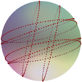
(a) $i_{k}$ is chosen in order

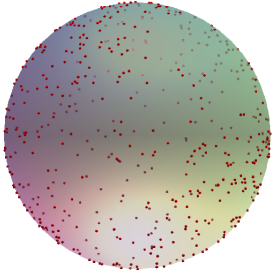
(b) $i_{k}$ is chosen in random

Figure 2: An illustration of the distribution of $\{{\bf x}_{0},{\bf x}_{1},\ldots,{\bf x}_{1000}\}$ on the sphere when $m=n=3$. The vectors are generated by the procedure (36).

The left one in Figure 2 describes the distribution of the vectors $\{{\bf x}_{i}:i=0,1,\ldots,1000\}$ generated by the procedure (36) with $i_{k}$ chosen in order, i.e., Algorithm 2. These vectors are located on six separate circles, each circle represents an ${\mathbb{S}}_{kj}$ defined in Section 3, and ${\mathbb{S}}_{k0}$ is parallel to ${\mathbb{S}}_{k1}$. The midpoint of the centers of ${\mathbb{S}}_{k0}$ and ${\mathbb{S}}_{k1}$ is the solution. This is confirmed by Theorem 7. The right one in Figure 2 shows the distribution of $\{{\bf x}_{i}:i=0,1,\ldots,1000\}$ generated by the process (36) with $i_{k}$ chosen with probability $\|A_{i_{k}}\|^{2}/\|A\|_{F}^{2}$, i.e., Steinerberger’s algorithm. The points are randomly distributed on the sphere. The average of them also provides a good approximation of the center of the sphere, i.e., a solution of the linear system $A{\bf x}={\bf b}$.

5.1 Comparison of $\eta(A)$ and $\kappa(A)$

The complexity of the deterministic iterative reflection algorithm depends on the parameter $\eta(A)$, while the complexities of previous Kaczmarz algorithms depend on the (scaled) condition number of $A$. As discussed after Proposition 11, for random Gaussian matrices, $\eta(A)$ has order $\kappa(A)$ instead of $\kappa^{2}(A)$. To see this more clearly, we numerically computed $\eta(A)$ and $\kappa(A)$ for around 10000 random matrices of size at most $1000\times 1000$ whose entries are independently taking values from the standard normal distribution. The numerical results suggest that there might be two constants $c_{0},c_{1}$ with $c_{0}\leq 0.55,c_{1}\geq 38.27$ such that $c_{0}\leq\kappa(A)/\eta(A)\leq c_{1}$. Although it is unclear about the dependence of the ratio $\kappa(A)/\eta(A)$ on the dimension theoretically, the numerical tests here suggest that these two quantities are often comparable.

5.2 Comparison of the four algorithms on random matrices

In this section, we show our testing results. All the calculations were done in the software Maple 2022 on MacBook Pro with processor 2.7 GHz Dual-Core Intel Core i5. The code is available at https://drive.google.com/file/d/1ZwzSh1Npgiw9nry6IjytkAvtW-wt6Jjh/view?usp=sharing. In the tests, we collected the total time the algorithms take to find a solution $\tilde{{\bf x}}$ of the linear system $A{\bf x}={\bf b}$ such that $\|A\tilde{{\bf x}}-{\bf b}\|\leq 0.01$. Since SA and DIR only apply to consistent linear systems, all the linear systems we generated are consistent. In the tests, we mainly focused on random matrices whose entries independently take values from the standard normal distribution. In the tests, for each case, we run 50 randomly generated examples and collect the average value of the runtime. All four algorithms start from the same initial vector, which is also generated randomly.

$m$	200	500	1000	1500	2000	5000	10000	15000	20000
SV	23.47	17.99	14.57	15.34	15.35	16.70	18.48	41.57	40.18
NT	16.83	9.73	7.29	6.53	7.46	6.79	5.75	6.43	4.45
SA	2.47	1.66	2.97	1.68	2.07	2.19	2.77	3.03	3.41
DIR	2.38	2.56	2.79	2.77	3.34	3.26	4.30	4.96	5.16

Table 2: The runtime (in seconds) of different Kaczmarz methods when $n=100$.

$m$	1000	1500	2000	2500	3000	3500	5000	10000	15000	20000
SV	73.84	51.46	40.32	41.73	41.14	41.76	50.84	141.23	147.53	225.57
NT	67.59	58.98	40.46	39.51	35.85	36.21	31.95	59.09	36.17	35.21
SA	6.47	6.26	5.83	6.71	8.55	9.33	10.16	18.45	24.27	26.97
DIR	7.54	7.33	7.11	8.27	11.21	12.29	13.65	22.05	25.81	29.84

Table 3: The runtime (in seconds) of different Kaczmarz methods when $n=300$.

	$M$	$2m$	$m$	$m/2$	$m/4$	$m/8$	$m/16$	$\lfloor m/32\rfloor$	$\lfloor m/64\rfloor$
$m=10000$	SA	22.11	12.39	10.45	9.73	6.50	5.14	2.63	4.34
$n=100$	DIR	21.78	12.82	10.43	9.05	5.96	3.04	5.01	10.34
$m=10000$	SA	120.13	58.52	41.85	26.05	17.87	14.45	14.31	23.15
$n=300$	DIR	115.51	57.86	36.95	26.43	22.05	34.95	75.12	654.14

Table 4: The influence of the number $M$ on SA and DIR. The unit of time is seconds.

From Tables 2 and 3, we can see that SA is slightly better than DIR, while the difference is not big. Both can compete with NT, which is further better than SV. Moreover, when the linear system is not so over-determined, SA and DIR seem to have better performance than NT. One uncertainty for SA and DIR is the quantity $M$, which determines how many samples we should generate before we restart further iterations. Let us assume that $m\gg n$. Denote $i=\lfloor\log(m/n)\rfloor$. From our numerical tests, we found that for SA, it is more efficient to use $M\in\{\lfloor m/2^{i-1}\rfloor,\lfloor m/2^{i}\rfloor\}$, and for DIR, $M\in\{\lfloor m/2^{i-2}\rfloor,\lfloor m/2^{i-1}\rfloor\}$ is better. In Table 4, we list some numerical results for this. We also found that for DIR, it is very slow if we set $M\leq n$ (e.g., see the last example in the fifth row of Table 4). This is not a problem for SA. But the efficiency of SA may be affected if $M\ll n$ (e.g., see the last example in the fourth row of Table 4). Both are inefficient when $M$ is too large.

6 Conclusions

In this paper, we proposed a new deterministic Kaczmarz algorithm by replacing orthogonal projections with reflections in the original Kaczmarz method. We established rigorous theorems about its correctness and efficiency. In this process, we discovered an interesting geometric fact about the solutions of consistent linear systems. Namely, any solution of a consistent linear system can be represented as the midpoint of the centers of two spheres. We feel it would be interesting to find more results from this fact. According to our numerical tests, the new Kaczmarz algorithm has a performance competitive with randomized Kaczmarz algorithms for consistent linear systems. However, it cannot be used to solve least-squares problems, which is partially caused by the structure of the algorithm. It would be interesting to find a way to fix this. Perhaps some new interesting geometric facts can be found in this way. Another interesting research topic is to find certain matrices such that $\eta(A)$ is small. In this paper, we found some partial results about its connection to the condition number. But this might be worth a systematic study. Finally, from our numerical experiments, Steinerberger’s algorithm works very well in practice. However, Steinerberger only studied the convergence rate in the nonsingular case. So it would be interesting to better understand this algorithm theoretically in the general case.

References

- [1] S. Agmon, The relaxation method for linear inequalities, Canadian Journal of Mathematics, 6 (1954), pp. 382–392.
- [2] J. R. Angelos, C. C. Cowen, and S. K. Narayan, Triangular truncation and finding the norm of a Hadamard multiplier, Linear Algebra and its Applications, 170 (1992), pp. 117–135.
- [3] R. Ansorge, Connections between the Cimmino-method and the Kaczmarz-method for the solution of singular and regular systems of equations, Computing, 33 (1984), pp. 367–375.
- [4] M. Benzi, Gianfranco Cimmino’s contributions to numerical mathematics, Atti del Seminario di Analisi Matematica, Dipartimento di Matematica dell’Universita di Bologna. Volume Speciale: Ciclo di Conferenze in Ricordo di Gianfranco Cimmino, (2004), pp. 87–109.
- [5] T. Brady and C. Watt, On products of Euclidean reflections, The American Mathematical Monthly, 113 (2006), pp. 826–829.
- [6] Y. Censor, Row-action methods for huge and sparse systems and their applications, SIAM review, 23 (1981), pp. 444–466.
- [7] Y. Censor, P. P. Eggermont, and D. Gordon, Strong underrelaxation in Kaczmarz’s method for inconsistent systems, Numerische Mathematik, 41 (1983), pp. 83–92.
- [8] J.-Q. Chen and Z.-D. Huang, On a fast deterministic block Kaczmarz method for solving large-scale linear systems, Numerical Algorithms, (2021), pp. 1–23.
- [9] G. Cimmino, Calcolo approssimato per le soluzioni dei sistemi di equazioni lineari, La Ricerca Scientifica, II (1938), pp. 326–333.
- [10] J. E. Cohen, H. Kesten, and C. M. Newman, Random Matrices and Their Applications: Proceedings of the AMS-IMS-SIAM Joint Summer Research Conference Held June 17-23, 1984, with Support from the National Science Foundation, vol. 50 of Contemporary mathematics, American Mathematical Society, Providence, Rhode Island, 1986.
- [11] F. Deutsch, Rate of Convergence of the Method of Alternating Projections, Birkhäuser Basel, Basel, 1985, pp. 96–107.
- [12] F. Deutsch and H. Hundal, The Rate of Convergence for the Method of Alternating Projections, II, Journal of Mathematical Analysis and Applications, 205 (1997), pp. 381–405.
- [13] A. Edelman, Eigenvalues and condition numbers of random matrices, SIAM journal on matrix analysis and applications, 9 (1988), pp. 543–560.
- [14] P. P. B. Eggermont, G. T. Herman, and A. Lent, Iterative algorithms for large partitioned linear systems, with applications to image reconstruction, Linear Algebra and its Applications, 40 (1981), pp. 37–67.
- [15] Y. C. Eldar and D. Needell, Acceleration of randomized Kaczmarz method via the Johnson–Lindenstrauss lemma, Numerical Algorithms, 58 (2011), pp. 163–177.
- [16] H. G. Feichtinger, C. Cenker, M. Mayer, H. Steier, and T. Strohmer, New variants of the pocs method using affine subspaces of finite codimension with applications to irregular sampling, in Visual Communications and Image Processing’92, vol. 1818, SPIE, 1992, pp. 299–310.
- [17] A. Galántai, On the rate of convergence of the alternating projection method in finite dimensional spaces, Journal of Mathematical Analysis and Applications, 310 (2005), pp. 30–44.
- [18] G. H. Golub and C. F. Van Loan, Matrix Computations, The Johns Hopkins University Press, fourth ed., 2013.
- [19] R. Gordon, R. Bender, and G. T. Herman, Algebraic Reconstruction Techniques (ART) for three-dimensional electron microscopy and X-ray photography, Journal of Theoretical Biology, 29 (1970), pp. 471–481.
- [20] R. Gower, D. Molitor, J. Moorman, and D. Needell, Adaptive sketch-and-project methods for solving linear systems, arXiv preprint arXiv:1909.03604, (2019).
- [21] R. M. Gower and P. Richtárik, Randomized iterative methods for linear systems, SIAM Journal on Matrix Analysis and Applications, 36 (2015), pp. 1660–1690.
- [22] C. Hildreth et al., A quadratic programming procedure, Naval research logistics quarterly, 4 (1957), pp. 79–85.
- [23] B. Jarman, N. Mankovich, and J. D. Moorman, Randomized extended kaczmarz is a limit point of sketch-and-project, arXiv preprint arXiv:2110.05605, (2021).
- [24] Y. Jiao, B. Jin, and X. Lu, Preasymptotic convergence of randomized Kaczmarz method, Inverse Problems, 33 (2017), p. 125012.
- [25] S. Karczmarz, Angenaherte auflosung von systemen linearer glei-chungen, Bull. Int. Acad. Pol. Sic. Let., Cl. Sci. Math. Nat., (1937), pp. 355–357.
- [26] A. Ma, D. Needell, and A. Ramdas, Convergence properties of the randomized extended Gauss–Seidel and Kaczmarz methods, SIAM Journal on Matrix Analysis and Applications, 36 (2015), pp. 1590–1604.
- [27] E. S. Meckes, The random matrix theory of the classical compact groups, vol. 218, Cambridge University Press, 2019.
- [28] J. D. Moorman, T. K. Tu, D. Molitor, and D. Needell, Randomized Kaczmarz with averaging, BIT Numerical Mathematics, 61 (2021), pp. 337–359.
- [29] T. S. Motzkin and I. J. Schoenberg, The relaxation method for linear inequalities, Canadian Journal of Mathematics, 6 (1954), pp. 393–404.
- [30] I. Necoara, Faster randomized block Kaczmarz algorithms, SIAM Journal on Matrix Analysis and Applications, 40 (2019), pp. 1425–1452.
- [31] D. Needell and J. A. Tropp, Paved with good intentions: analysis of a randomized block Kaczmarz method, Linear Algebra and its Applications, 441 (2014), pp. 199–221.
- [32] D. Needell, R. Ward, and N. Srebro, Stochastic gradient descent, weighted sampling, and the randomized Kaczmarz algorithm, Advances in neural information processing systems, 27 (2014), pp. 1017–1025.
- [33] D. Needell, R. Zhao, and A. Zouzias, Randomized block Kaczmarz method with projection for solving least squares, Linear Algebra and its Applications, 484 (2015), pp. 322–343.
- [34] Y.-Q. Niu and B. Zheng, A greedy block Kaczmarz algorithm for solving large-scale linear systems, Applied Mathematics Letters, 104 (2020), p. 106294.
- [35] J. Nutini, B. Sepehry, A. Virani, I. Laradji, M. Schmidt, and H. Koepke, Convergence rates for greedy kaczmarz algorithms, in Conference on Uncertainty in Artificial Intelligence, 2016.
- [36] S. Petra and C. Popa, Single projection Kaczmarz extended algorithms, Numerical Algorithms, 73 (2016), pp. 791–806.
- [37] P. Richtárik and M. Takác, Stochastic reformulations of linear systems: algorithms and convergence theory, SIAM Journal on Matrix Analysis and Applications, 41 (2020), pp. 487–524.
- [38] C. Shao and A. Montanaro, Faster quantum-inspired algorithms for solving linear systems, ACM Transactions on Quantum Computing, 3 (2022), pp. 1–23.
- [39] C. Shao and H. Xiang, Row and column iteration methods to solve linear systems on a quantum computer, Physical Review A, 101 (2020), p. 022322.
- [40] S. Steinerberger, Surrounding the solution of a linear system of equations from all sides, Quarterly of Applied Mathematics, 79 (2021), pp. 419–429.
- [41] T. Strohmer and R. Vershynin, A randomized Kaczmarz algorithm with exponential convergence, Journal of Fourier Analysis and Applications, 15 (2009), pp. 262–278.
- [42] K. Tanabe, Projection method for solving a singular system of linear equations and its applications, Numerische Mathematik, 17 (1971), pp. 203–214.
- [43] T. Tao and V. Vu, Smooth analysis of the condition number and the least singular value, Mathematics of computation, 79 (2010), pp. 2333–2352.
- [44] N. Wu and H. Xiang, Projected randomized Kaczmarz methods, Journal of Computational and Applied Mathematics, 372 (2020), p. 112672.
- [45] H. Xiang and L. Zhang, Randomized iterative methods with alternating projections, arXiv preprint arXiv:1708.09845, (2017).
- [46] Y. Yaniv, J. D. Moorman, W. Swartworth, T. Tu, D. Landis, and D. Needell, Selectable Set Randomized Kaczmarz, arXiv preprint arXiv:2110.04703, (2021).
- [47] A. Zouzias and N. M. Freris, Randomized extended Kaczmarz for solving least squares, SIAM Journal on Matrix Analysis and Applications, 34 (2013), pp. 773–793.