Optimal Spatial Signal Design for mmWave Positioning under Imperfect Synchronization

Abstract

We consider the problem of spatial signal design for multipath-assisted mmWave positioning under limited prior knowledge on the user’s location and clock bias. We propose an optimal robust design and, based on the low-dimensional precoder structure under perfect prior knowledge, a codebook-based heuristic design with optimized beam power allocation. Through numerical results, we characterize different position-error-bound (PEB) regimes with respect to clock bias uncertainty and show that the proposed low-complexity codebook-based designs outperform the conventional directional beam codebook and achieve near-optimal PEB performance for both analog and digital architectures.

I Introduction

In 5G mmWave systems, in addition to time-of-arrival (TOA) measurements, the ability to estimate angles-of-arrival (AOAs) and angles-of-departure (AODs) has been introduced [1], which provides additional geometric information, increases multipath resolvability and enables the exploitation of reflected propagation paths to improve positioning, in contrast to sub-6 GHz systems. Based on the combination of TOA, AOA and AOD measurements, joint positioning and synchronization with a single BS can be realized under multipath conditions [2]. In contrast to positioning signals in time and frequency [3, Section 7.4.1.7], spatial positioning signals are inherently directional and thus mainly meaningful under a-priori information about the location of the user equipment (UE), which can be obtained in a tracking scenario [4, 2]. Conventional spatial signal design at the BS involves a set of directional beams (e.g., from a DFT codebook), where the reported received power at the UE reveals a coarse AOD information [5].

With the advent of digital and hybrid arrays, more refined spatial designs that boost localization performance become possible [6, 7, 8]. In [6], the authors adopt the Cramér-Rao bound (CRB) as a design criterion and optimize the AOA and AOD accuracy under pure line-of-sight (LOS) propagation by exploiting prior knowledge on UE location. Similarly, [7] proposes an iterative signal design approach to minimize the CRB on location estimation in the presence of both LOS and NLOS paths, which requires multiple rounds of localization and signal optimization, thus causing significant overhead. The studies in [6, 7] share two major limitations, namely, (i) the high-complexity of the unconstrained design (i.e., without a specific codebook), and (ii) the impractical assumption of perfect synchronization between BS and UE [2]. To address such limitations, [8] considers a mmWave localization setup with clock offset between BS and UE, and designs codebook-based spatial signals containing only conventional directional beams. However, the prior approaches to signal design [6, 7, 8] leave undiscovered whether (i) novel codebooks with alternative beams in addition to directional ones can be devised to improve accuracy over standard codebooks, (ii) the localization performance of codebook-based designs can approach that of unconstrained ones, and (iii) analog beams can achieve similar performance to digital ones.

With the goal of tackling the above issues, we consider the design of both unconstrained and codebook-based spatial signals for 5G and beyond 5G multipath-assisted mmWave positioning under limited prior knowledge on UE location [4, 6, 2] and imperfect synchronization in analog and digital arrays. Our main contributions are: (i) We derive the structure of the optimal spatial signals under perfect prior knowledge on the UE location [9], establishing an insightful connection to monopulse radar [10]; (ii) Inspired by the low-dimensional structure of these optimal signals, we propose a novel low-complexity codebook-based design under imperfect prior knowledge, involving both directional and derivative beams, and an optimal unconstrained design; (iii) We characterize different position-error-bound (PEB) regimes with respect to clock bias uncertainty, providing practical guidelines on which spatial signal to use under different levels of synchronization; (iv) We show that the proposed low-complexity codebook can be implemented in an analog architecture, outperforms the codebook with only directional beams [8], and attains the upper bound specified by the unconstrained design.

II System Model and Problem Description

Signal Model

Consider a MIMO-OFDM mmWave downlink communications scenario with a BS and a single UE (as in [6, 7, 8]), equipped with $N_{\rm{Tx}}$ and $N_{\rm{Rx}}$ antennas, respectively. Having an architecture with the capability of transmitting scaled and phase-shifted versions of signal across the different antennas, the BS transmits $M$ identical pilot frames sequentially, where each frame $\mathbf{S}\in\mathbb{C}^{K\times L}$ consists of $L$ OFDM symbols with $K$ subcarriers, each representing a time-frequency comb pattern [1, 3]. Assuming that the ${{m^{\rm{th}}}}$ pilot frame is precoded by a vector $\mathbf{f}_{m}\in\mathbb{C}^{N_{\rm{Tx}}\times 1}$ for $m=0,1,\ldots,M-1$, the received signal vector at the UE over the ${{k^{\rm{th}}}}$ subcarrier of the ${{\ell^{\rm{th}}}}$ symbol in the ${{m^{\rm{th}}}}$ frame can be expressed as [6]

$$\mathbf{y}_{k,\ell,m}=\mathbf{W}^{H}\mathbf{H}_{k}\mathbf{f}_{m}s_{k,\ell}+\mathbf{n}_{k,\ell,m}\leavevmode\nobreak\ ,$$ (1)

for $k=0,\ldots,K-1$, $\ell=0,\ldots,L-1$, where $\mathbf{W}\in\mathbb{C}^{N_{\rm{Rx}}\times N_{{\rm{RF}}}}$ is the analog combining matrix at the UE, with $N_{{\rm{RF}}}$ denoting the number of RF chains, $s_{k,\ell}=\left[\mathbf{S}\right]_{k,\ell}$ is the pilot symbol on the ${{k^{\rm{th}}}}$ subcarrier of the ${{\ell^{\rm{th}}}}$ symbol, $\mathbf{H}_{k}\in\mathbb{C}^{N_{\rm{Rx}}\times N_{\rm{Tx}}}$ is the channel matrix at the ${{k^{\rm{th}}}}$ subcarrier, given by

$$\mathbf{H}_{k}=\sum_{{\color[rgb]{0,0,0}g}=0}^{{\color[rgb]{0,0,0}G}-1}\alpha_{{\color[rgb]{0,0,0}g}}\,e^{-j2\pi k\Delta f\tau_{{\color[rgb]{0,0,0}g}}}\mathbf{a}_{\rm{Rx}}(\phi_{{\color[rgb]{0,0,0}g}})\mathbf{a}_{\rm{Tx}}^{T}(\theta_{{\color[rgb]{0,0,0}g}})\leavevmode\nobreak\ ,$$ (2)

and $\mathbf{n}_{k,\ell,m}\sim{\mathcal{CN}}({{\bm{0}}},\sigma^{2}{\bm{\mathrm{I}}})$ is additive white Gaussian noise. Here, $\Delta f$ is the subcarrier spacing, $G$ denotes the number of paths, $\alpha_{{\color[rgb]{0,0,0}g}}$, $\tau_{{\color[rgb]{0,0,0}g}}$, $\phi_{{\color[rgb]{0,0,0}g}}$ and $\theta_{{\color[rgb]{0,0,0}g}}$ are the complex channel gain, delay, AOA and AOD of the ${{{\color[rgb]{0,0,0}g}^{\rm{th}}}}$ path, respectively, and $\mathbf{a}_{\rm{Tx}}(\theta)\in\mathbb{C}^{N_{\rm{Tx}}\times 1}$ and $\mathbf{a}_{\rm{Rx}}(\phi)\in\mathbb{C}^{N_{\rm{Rx}}\times 1}$ denote the array steering vectors at the BS and UE, respectively.

System Geometry

We consider a 2D positioning setup (see Fig. 1) where the BS and UE are located at $\mathbf{q}=\left[q_{x},q_{y}\right]^{T}\in\mathbb{R}^{2\times 1}$ and $\mathbf{p}=\left[p_{x},p_{y}\right]^{T}\in\mathbb{R}^{2\times 1}$, respectively, and the orientation of the UE is denoted by $\psi\in[0,2\pi)$. We assume that $\mathbf{q}$ is known, while $\mathbf{p}$ and $\psi$ are unknown to be estimated from (1), as in [11, 12]. For the channel model, ${{\color[rgb]{0,0,0}g}}=0$ represents the LOS path, while ${{\color[rgb]{0,0,0}g}}\geq 1$ correspond to the NLOS paths. Each NLOS path is associated with an incidence point with unknown location $\mathbf{r}_{{\color[rgb]{0,0,0}g}}=\left[r_{{{\color[rgb]{0,0,0}g}},x},r_{{{\color[rgb]{0,0,0}g}},y}\right]^{T}\in\mathbb{R}^{2\times 1}$. According to the system geometry, the angles can be expressed as

$$\theta_{{{\color[rgb]{0,0,0}g}}>0} ={\rm{atan2}}(r_{{{\color[rgb]{0,0,0}g}},y}-q_{y},r_{{{\color[rgb]{0,0,0}g}},x}-q_{x})\leavevmode\nobreak\ ,$$ (3)

$$\theta_{0} ={\rm{atan2}}(p_{y}-q_{y},p_{x}-q_{x})\leavevmode\nobreak\ ,$$ (4)

$$\phi_{{{\color[rgb]{0,0,0}g}}>0} ={\rm{atan2}}(p_{y}-r_{{{\color[rgb]{0,0,0}g}},y},p_{x}-r_{{{\color[rgb]{0,0,0}g}},x})-\psi\leavevmode\nobreak\ ,$$ (5)

$$\phi_{0} =\theta_{0}-\psi,$$ (6)

with ${\rm{atan2}}(y,x)$ denoting the four-quadrant inverse tangent. The path delays are given by

$$\tau_{{{\color[rgb]{0,0,0}g}}>0} =(\left\lVert\mathbf{q}-\mathbf{r}_{{\color[rgb]{0,0,0}g}}\right\rVert_{2}+\left\lVert\mathbf{r}_{{\color[rgb]{0,0,0}g}}-\mathbf{p}\right\rVert_{2})/c+\Delta t\leavevmode\nobreak\ ,$$ (7)

$$\tau_{0} =\left\lVert\mathbf{p}-\mathbf{q}\right\rVert_{2}/c+\Delta t,$$ (8)

where $c$ is the speed of propagation and $\Delta t$ is the clock bias between the BS and UE, modeled as $\Delta t\sim p(\Delta t)$.

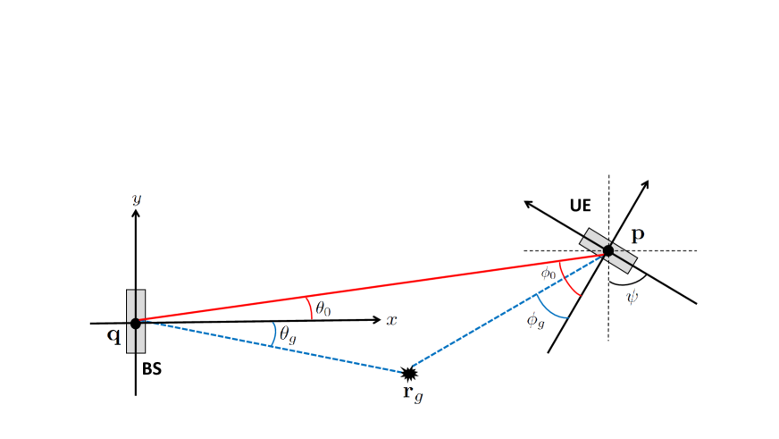
Figure 1: 2D geometric model of mmWave MIMO positioning setup with known BS position $\mathbf{q}$, unknown UE location $\mathbf{p}$ and orientation $\psi$, and unknown incidence point location $\mathbf{r}_{{\color[rgb]{0,0,0}g}}$.

Problem Description for Spatial Signal Design

Our problem of interest for mmWave spatial signal design is to find the optimal (analog, hybrid, or digital) precoder $\mathbf{F}\triangleq\left[\mathbf{f}_{0}\,\ldots\,\mathbf{f}_{M-1}\right]\in\mathbb{C}^{N_{\rm{Tx}}\times M}$ that maximizes the accuracy of estimation of UE location $\mathbf{p}$ in a setup where also the orientation $\psi$, the clock bias $\Delta t$ and the incidence point locations $\{\mathbf{r}_{{\color[rgb]{0,0,0}g}}\}_{{\color[rgb]{0,0,0}g}=1}^{{\color[rgb]{0,0,0}G}-1}$ have to be estimated. The input data for the estimator are the observations $\{\mathbf{y}_{k,\ell,m}\}_{\forall k,\ell,m}$ in (1), collected over $M$ beams each employing $L$ symbols with $K$ subcarriers, together with the prior knowledge on $\mathbf{p}$, $\{\mathbf{r}_{{\color[rgb]{0,0,0}g}}\}_{{{\color[rgb]{0,0,0}g}}=1}^{{{\color[rgb]{0,0,0}G}}-1}$ and $\Delta t$. Since the BS has no control over the UE, $\mathbf{W}$ is assumed to be fixed and not subject to optimization.

III Spatial Signal Design for mmWave Positioning

In this section, we derive the CRB based performance metric for position estimation, and propose unconstrained and codebook-based strategies to design spatial signals.

III-A CRB-Based Performance Metric

The channel and location domain unknown parameter vectors are given by ${\bm{\eta}}=\left[\bm{\theta}^{T},\bm{\phi}^{T},\bm{\alpha}_{\rm{R}}^{T},\bm{\alpha}_{\rm{I}}^{T},\bm{\tau}^{T}\right]^{T}\in\mathbb{R}^{5{\color[rgb]{0,0,0}G}\times 1}$ and ${\bm{\widetilde{\eta}}}=[\mathbf{p}^{T},\psi,\mathbf{r}^{T},\bm{\alpha}_{\rm{R}}^{T},\bm{\alpha}_{\rm{I}}^{T},\Delta t]^{T}\in\mathbb{R}^{(4{\color[rgb]{0,0,0}G}+2)\times 1}$, respectively, where $\bm{\theta}=\left[\theta_{0},\ldots,\theta_{{\color[rgb]{0,0,0}G}-1}\right]^{T}$, $\bm{\phi}=\left[\phi_{0},\ldots,\phi_{{\color[rgb]{0,0,0}G}-1}\right]^{T}$, $\bm{\alpha}_{\rm{R}}=\left[\Re\left\{\alpha_{0}\right\},\ldots,\Re\left\{\alpha_{{\color[rgb]{0,0,0}G}-1}\right\}\right]^{T}$, $\bm{\alpha}_{\rm{I}}=\left[\Im\left\{\alpha_{0}\right\},\ldots,\Im\left\{\alpha_{{\color[rgb]{0,0,0}G}-1}\right\}\right]^{T}$, $\bm{\tau}=\left[\tau_{0},\ldots,\tau_{{\color[rgb]{0,0,0}G}-1}\right]^{T}$ and $\mathbf{r}=[\mathbf{r}_{1}^{T},\ldots,\mathbf{r}_{{\color[rgb]{0,0,0}G}-1}^{T}]^{T}$. The Fisher information matrix (FIM) $\mathbf{J}\in\mathbb{R}^{5{\color[rgb]{0,0,0}G}\times 5{\color[rgb]{0,0,0}G}}$ of ${\bm{\eta}}$ can be computed from the signal model in (1) using the Slepian-Bangs formula [13, Eq. (15.52)] as

$$\left[\mathbf{J}\right]_{i,j}=\frac{2}{\sigma^{2}}\sum_{k=0}^{K-1}\sum_{\ell=0}^{L-1}\sum_{m=0}^{M-1}\Re\left\{\frac{\partial\macc@depth\char 1\relax\frozen@everymath{\macc@group}\macc@set@skewchar\macc@nested@a 111{\mathbf{y}}_{k,\ell,m}^{H}}{\partial\eta_{i}}\frac{\partial\macc@depth\char 1\relax\frozen@everymath{\macc@group}\macc@set@skewchar\macc@nested@a 111{\mathbf{y}}_{k,\ell,m}}{\partial\eta_{j}}\right\}$$ (9)

for $i,j=0,\ldots,5{\color[rgb]{0,0,0}G}-1$, where $\macc@depth\char 1\relax\frozen@everymath{\macc@group}\macc@set@skewchar\macc@nested@a 111{\mathbf{y}}_{k,\ell,m}=\mathbf{W}^{H}\mathbf{H}_{k}\mathbf{f}_{m}s_{k,\ell}$.

Since our focus is on the positioning performance, we derive the FIM $\widetilde{\mathbf{J}}\in\mathbb{R}^{(4{\color[rgb]{0,0,0}G}+2)\times(4{\color[rgb]{0,0,0}G}+2)}$ of ${\bm{\widetilde{\eta}}}$ as

$$\widetilde{\mathbf{J}}=\mathbf{T}^{T}\mathbf{J}\mathbf{T}+\mathbf{J}^{\rm{prior}}\leavevmode\nobreak\ ,$$ (10)

where $\mathbf{T}^{T}\mathbf{J}\mathbf{T}$ and $\mathbf{J}^{\rm{prior}}$ represent the FIMs derived from the observations and the prior knowledge, respectively, and the transformation matrix $\mathbf{T}\in\mathbb{R}^{5{\color[rgb]{0,0,0}G}\times(4{\color[rgb]{0,0,0}G}+2)}$ can be expressed as the Jacobian $[\mathbf{T}]_{i,j}=\partial[{\bm{\eta}}]_{i}/\partial[{\bm{\widetilde{\eta}}}]_{j}$. Since only the clock bias is assumed to be random in ${\bm{\widetilde{\eta}}}$, we have $\left[\mathbf{J}^{\rm{prior}}\right]_{(4{\color[rgb]{0,0,0}G}+2,4{\color[rgb]{0,0,0}G}+2)}=J_{\rm{clk}}\geq 0$, derived from $p(\Delta t)$, and all other entries of $\mathbf{J}^{\rm{prior}}$ are zero [12]. To quantify the position estimation accuracy, we adopt the PEB as our performance metric, which can be computed via [11, 12]

$${\rm{PEB}}(\mathbf{F};{\bm{\widetilde{\eta}}})=\left[{{{\rm{tr}}\left([\widetilde{\mathbf{J}}^{-1}]_{0:1,0:1}\right)}}\right]^{1/2}\leavevmode\nobreak\ .$$ (11)

As seen from Appendix A, the FIM $\widetilde{\mathbf{J}}$ and the PEB in (11) are functions of the precoder $\mathbf{F}$ employed by the BS.

III-B Optimal Signal Design with Perfect Knowledge

The PEB depends on the deterministic unknown parameters in ${\bm{\widetilde{\eta}}}$ (i.e., $\mathbf{p}$, $\psi$, $\mathbf{r}$, $\bm{\alpha}_{\rm{R}}$ and $\bm{\alpha}_{\rm{I}}$). In this part, we assume perfect knowledge of these parameters and formulate the signal design problem accordingly. In Sec. III-C, we will focus on robust signal design in the presence of uncertainties in ${\bm{\widetilde{\eta}}}$. Under perfect knowledge of ${\bm{\widetilde{\eta}}}$, the signal design problem with a total power constraint ${P_{\rm{tot}}}$ can be formulated as

$$\mathop{\mathrm{min}}\limits_{\mathbf{F}} \leavevmode\nobreak\ \leavevmode\nobreak\ {\rm{PEB}}(\mathbf{F};{\bm{\widetilde{\eta}}})\leavevmode\nobreak\ \leavevmode\nobreak\ \mathrm{s.t.}\leavevmode\nobreak\ \leavevmode\nobreak\ {{{\rm{tr}}\left(\mathbf{F}\mathbf{F}^{H}\right)}}={\color[rgb]{0,0,0}{P_{\rm{tot}}}/(KL)}\leavevmode\nobreak\ .$$ (12)

Using change of variables $\mathbf{X}={\color[rgb]{0,0,0}L}\mathbf{F}\mathbf{F}^{H}$, (12) can be relaxed to (by removing the constraint ${\rm{rank}}(\mathbf{X})=M$) [14, Ch. 7.5.2]

$$\mathop{\mathrm{min}}\limits_{\mathbf{X},\mathbf{u}} \leavevmode\nobreak\ \leavevmode\nobreak\ {{\bm{1}}}^{T}\mathbf{u}$$ (13)

$$\mathrm{s.t.} \leavevmode\nobreak\ \leavevmode\nobreak\ \begin{bmatrix}\widetilde{\mathbf{J}}{\color[rgb]{0,0,0}(\mathbf{X})}&\mathbf{e}_{b}\\ \mathbf{e}^{T}_{b}&u_{b}\end{bmatrix}\succeq 0,\leavevmode\nobreak\ b=0,1,\leavevmode\nobreak\ {{{\rm{tr}}\left(\mathbf{X}\right)}}={\color[rgb]{0,0,0}\frac{{P_{\rm{tot}}}}{K}},\mathbf{X}\succeq 0\leavevmode\nobreak\ ,$$

where $\mathbf{u}=\left[u_{0},u_{1}\right]^{T}$ is a newly introduced auxiliary variable and $\mathbf{e}_{b}$ is the ${{b^{\rm{th}}}}$ column of the identity matrix. It can be observed from Appendix A and (10) that $\widetilde{\mathbf{J}}{\color[rgb]{0,0,0}(\mathbf{X})}$ is a linear function of $\mathbf{X}$ [9, 6], which implies that (13) is a convex semidefinite program (SDP) [14, Ex. 3.26] and thus can be solved via standard convex optimization tools. The following proposition provides the structure of the precoder covariance matrix for the relaxed problem in (13).

Proposition 1.

The precoder covariance matrix $\mathbf{X}^{\star}$ obtained as the solution to the relaxed problem in (13) can be expressed as

$$\mathbf{X}^{\star}=\mathbf{U}_{{\rm{Tx}}}\mathbf{\Lambda}\mathbf{U}_{{\rm{Tx}}}^{H}\leavevmode\nobreak\ ,$$ (14)

where $\mathbf{\Lambda}\in\mathbb{C}^{2{\color[rgb]{0,0,0}G}\times 2{\color[rgb]{0,0,0}G}}$ is a positive semidefinite (PSD) matrix and $\mathbf{U}_{{\rm{Tx}}}\triangleq[\mathbf{A}_{{\rm{Tx}}}\leavevmode\nobreak\ \accentset{\mbox{\large.}}{\mathbf{A}}_{{{\rm{Tx}}}}]^{*}$, $\mathbf{A}_{{\rm{Tx}}}\triangleq[\mathbf{a}_{\rm{Tx}}(\theta_{0})\,\ldots\,\mathbf{a}_{\rm{Tx}}(\theta_{{\color[rgb]{0,0,0}G}-1})]$, $\accentset{\mbox{\large.}}{\mathbf{A}}_{{{\rm{Tx}}}}\triangleq[\accentset{\mbox{\large.}}{\mathbf{a}}_{{{\rm{Tx}}}}(\theta_{0})\,\ldots\,\accentset{\mbox{\large.}}{\mathbf{a}}_{{{\rm{Tx}}}}(\theta_{{\color[rgb]{0,0,0}G}-1})]$, with $\accentset{\mbox{\large.}}{\mathbf{a}}_{{{\rm{Tx}}}}(\theta)\triangleq{\partial\mathbf{a}_{\rm{Tx}}(\theta)}/{\partial\theta}$.

Proof 0.

See Appendix B.

Proposition 1 can significantly reduce the computational burden of solving (13) since the optimization can equivalently be performed over $\mathbf{\Lambda}\in\mathbb{C}^{2{\color[rgb]{0,0,0}G}\times 2{\color[rgb]{0,0,0}G}}$ instead of $\mathbf{X}\in\mathbb{C}^{N_{\rm{Tx}}\times N_{\rm{Tx}}}$. Note that due to channel sparsity in mmWave [16], we usually have ${\color[rgb]{0,0,0}G}\ll N_{\rm{Tx}}$. Hence, we propose to solve the following equivalent convex problem:

$$\mathop{\mathrm{min}}\limits_{\mathbf{\Lambda},\mathbf{u}}\leavevmode\nobreak\ {{\bm{1}}}^{T}\mathbf{u}\quad\mathrm{s.t.} \begin{bmatrix}\widetilde{\mathbf{J}}{\color[rgb]{0,0,0}(\mathbf{\Lambda})}&\mathbf{e}_{b}\\ \mathbf{e}^{T}_{b}&u_{b}\end{bmatrix}\succeq 0,b=0,1,$$ (15)

$${{{\rm{tr}}\left(\mathbf{U}_{{\rm{Tx}}}\mathbf{\Lambda}\mathbf{U}_{{\rm{Tx}}}^{H}\right)}}={\color[rgb]{0,0,0}\frac{{P_{\rm{tot}}}}{K}},\mathbf{\Lambda}\succeq 0.$$

Based on Proposition 1, it is worth highlighting the remarkable connection between mmWave positioning and monopulse radar [10]. Precisely, $\mathbf{A}_{{\rm{Tx}}}$ and $\accentset{\mbox{\large.}}{\mathbf{A}}_{{{\rm{Tx}}}}$ correspond to sum and difference beams employed in monopulse radar for target tracking with high precision. In the context of mmWave signal design, UE can be tracked by using a combination of directional and derivative beams pointing towards the path AODs. The key difference is that a mmWave BS can exploit multipath to enable positioning under imperfect BS-UE synchronization while monopulse radar relies on LOS-only tracking with narrow beamwidth (i.e., $\mathbf{A}_{{\rm{Tx}}}$ and $\accentset{\mbox{\large.}}{\mathbf{A}}_{{{\rm{Tx}}}}$ contain a single beam in a monopulse system [10]). Fig. 2 illustrates the beampatterns of directional and derivative beams, which agree with those of sum and difference beams in [10, Fig. 2].

III-C Robust Signal Design with Imperfect Knowledge

Assuming that ${\bm{\widetilde{\eta}}}$ belongs to an uncertainty region $\mathcal{U}$ [6], we propose two strategies for robust signal design. In practice, $\mathcal{U}$ can be determined from the output of tracking routines, where the means and covariances of the parameters specify, respectively, the center and the extent of $\mathcal{U}$ [2].

III-C1 Optimization-Based Robust Unconstrained Design

Under imperfect knowledge of ${\bm{\widetilde{\eta}}}$, we resort to the worst-case PEB minimization strategy:

$$\mathop{\mathrm{min}}\limits_{\mathbf{X}} \leavevmode\nobreak\ \leavevmode\nobreak\ \mathop{\mathrm{max}}\limits_{{\bm{\widetilde{\eta}}}\in\mathcal{U}}\leavevmode\nobreak\ {\rm{PEB}}(\mathbf{X};{\bm{\widetilde{\eta}}})\leavevmode\nobreak\ \leavevmode\nobreak\ \mathrm{s.t.}\leavevmode\nobreak\ \leavevmode\nobreak\ {{{\rm{tr}}\left(\mathbf{X}\right)}}={\color[rgb]{0,0,0}\frac{{P_{\rm{tot}}}}{K}},\leavevmode\nobreak\ \mathbf{X}\succeq 0\leavevmode\nobreak\ .$$ (16)

Discretizing $\mathcal{U}$ into a uniform grid of $N$ points $\{{\bm{\widetilde{\eta}}}_{n}\}_{n=0}^{N-1}$, the problem in (16) can be reformulated in the epigraph form as

$$\mathop{\mathrm{min}}\limits_{\mathbf{X},t,\{u_{n,b}\}}\leavevmode\nobreak\ t$$ (17)

$$\mathrm{s.t.}\leavevmode\nobreak\ \begin{bmatrix}\widetilde{\mathbf{J}}({\color[rgb]{0,0,0}\mathbf{X}};{\bm{\widetilde{\eta}}}_{n})&\mathbf{e}_{b}\\ \mathbf{e}^{T}_{b}&u_{n,b}\end{bmatrix}\succeq 0,\leavevmode\nobreak\ b=0,1,\leavevmode\nobreak\ n=0,\ldots,N-1$$

$$\hskip 19.91692ptu_{n,0}+u_{n,1}\leq t,\leavevmode\nobreak\ n=0,\ldots,N-1$$

$$\hskip 19.91692pt{{{\rm{tr}}\left(\mathbf{X}\right)}}={\color[rgb]{0,0,0}{P_{\rm{tot}}}/K},\leavevmode\nobreak\ \mathbf{X}\succeq 0,$$

where $\widetilde{\mathbf{J}}({\color[rgb]{0,0,0}\mathbf{X};}{\bm{\widetilde{\eta}}}_{n})$ represents the FIM in (10) evaluated at ${\bm{\widetilde{\eta}}}={\bm{\widetilde{\eta}}}_{n}$, and $t$ and $\{u_{n,b}\}_{\forall n,b}$ are auxiliary variables. Similar to (13), the problem in (17) is an SDP and can be solved using convex optimization [17].

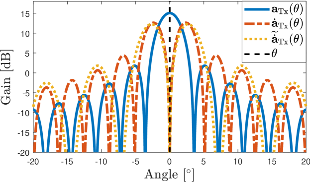
Figure 2: Uniform linear array (ULA) beampatterns of the directional beam $\mathbf{a}_{\rm{Tx}}(\theta)$, the digital derivative beam $\accentset{\mbox{\large.}}{\mathbf{a}}_{{{\rm{Tx}}}}(\theta)$ and the analog derivative beam $\widetilde{\accentset{\mbox{\large.}}{\mathbf{a}}}_{{{\rm{Tx}}}}(\theta)$ for $\theta=0$ with $N_{\rm{Tx}}=32$ antennas. Intuitively, the directional beam provides the required SNR for position estimation, while the derivative beam helps the UE to best identify small deviations from the boresight direction, like in monopulse radar, as evidenced by its sharp curvature around the boresight. High-precision tracking of UE involves weighted combination of directional and derivative beams.

III-C2 Codebook-Based Heuristic Design with Optimized Beam Power Allocation

Due to the presence of multiple grid points $\{{\bm{\widetilde{\eta}}}_{n}\}_{n=0}^{N-1}$, (17) cannot be transformed into a lower dimensional problem, as in (15). To devise a low-complexity signal design approach as an alternative to the SDP in (17), we propose a codebook-based heuristic design inspired by Proposition 1. Specifically, we consider the following digital and analog codebooks to span the AOD uncertainty intervals of the different paths:

$$\vspace{-0.2in}\mathbf{F}^{\rm{digital}}\triangleq\left[\mathbf{F}^{\rm{sum}}\leavevmode\nobreak\ \mathbf{F}^{\rm{diff}}\right]\,,\leavevmode\nobreak\ \mathbf{F}^{\rm{analog}}\triangleq\left[\mathbf{F}^{\rm{sum}}\leavevmode\nobreak\ \widetilde{\mathbf{F}}^{\rm{diff}}\right]\leavevmode\nobreak\ ,$$ (18)

where $\mathbf{F}^{\rm{sum}}\triangleq\left[\mathbf{F}^{\rm{sum}}_{0}\,\ldots\,\mathbf{F}^{\rm{sum}}_{{{\color[rgb]{0,0,0}G}}-1}\right]$, $\mathbf{F}^{\rm{diff}}\triangleq\left[\mathbf{F}^{\rm{diff}}_{0}\,\ldots\,\mathbf{F}^{\rm{diff}}_{{{\color[rgb]{0,0,0}G}}-1}\right]$, $\widetilde{\mathbf{F}}^{\rm{diff}}\triangleq\left[\widetilde{\mathbf{F}}^{\rm{diff}}_{0}\,\ldots\,\widetilde{\mathbf{F}}^{\rm{diff}}_{{{\color[rgb]{0,0,0}G}}-1}\right]$, in which

$$\vspace{-0.2in}\mathbf{F}^{\rm{sum}}_{{\color[rgb]{0,0,0}g}} \triangleq\left[\mathbf{a}_{\rm{Tx}}(\theta_{{{\color[rgb]{0,0,0}g}},0})\,\ldots\,\mathbf{a}_{\rm{Tx}}(\theta_{{{\color[rgb]{0,0,0}g}},N_{{\color[rgb]{0,0,0}g}}-1})\right]\leavevmode\nobreak\ ,$$ (19)

$$\mathbf{F}^{\rm{diff}}_{{\color[rgb]{0,0,0}g}} \triangleq\left[\accentset{\mbox{\large.}}{\mathbf{a}}_{{{\rm{Tx}}}}(\theta_{{{\color[rgb]{0,0,0}g}},0})\,\ldots\,\accentset{\mbox{\large.}}{\mathbf{a}}_{{{\rm{Tx}}}}(\theta_{{{\color[rgb]{0,0,0}g}},N_{{\color[rgb]{0,0,0}g}}-1})\right]\leavevmode\nobreak\ ,$$ (20)

$$\widetilde{\mathbf{F}}^{\rm{diff}}_{{\color[rgb]{0,0,0}g}} \triangleq\left[\widetilde{\accentset{\mbox{\large.}}{\mathbf{a}}}_{{{\rm{Tx}}}}(\theta_{{{\color[rgb]{0,0,0}g}},0})\,\ldots\,\widetilde{\accentset{\mbox{\large.}}{\mathbf{a}}}_{{{\rm{Tx}}}}(\theta_{{{\color[rgb]{0,0,0}g}},N_{{\color[rgb]{0,0,0}g}}-1})\right]\leavevmode\nobreak\ ,$$ (21)

for ${{\color[rgb]{0,0,0}g}}\in\{0,\ldots,{{\color[rgb]{0,0,0}G}}-1\}$. Here, $\{\theta_{{{\color[rgb]{0,0,0}g}},i}\}_{i=0}^{N_{{\color[rgb]{0,0,0}g}}-1}$ denote the evenly spaced AODs covering the uncertainty interval of the ${{{{\color[rgb]{0,0,0}g}}^{\rm{th}}}}$ path, with an angular spacing equal to $3\,\rm{dB}$ (half-power) beamwidth [18], [19, Ch. 22.10]. Moreover, $\widetilde{\accentset{\mbox{\large.}}{\mathbf{a}}}_{{{\rm{Tx}}}}(\theta)$ denotes the best analog approximation (i.e., with unit-modulus entries) to $\accentset{\mbox{\large.}}{\mathbf{a}}_{{{\rm{Tx}}}}(\theta)$ determined using gradient projections iterations in [20, Alg. 1]. In (18), $\mathbf{F}^{\rm{sum}}$ represents a standard directional beam codebook, while $\mathbf{F}^{\rm{diff}}$ and $\widetilde{\mathbf{F}}^{\rm{diff}}$ are novel derivative codebooks stemming from Proposition 1. Note that in the regime of large number of antennas, broader beams than steering vectors should be used to avoid very large $N_{{\color[rgb]{0,0,0}g}}$.

Table I: Simulation Parameters

$f_{c}$	$28\,\rm{GHz}$	BS loc. $\mathbf{q}$	$\left[0,0\right]\leavevmode\nobreak\ \rm{m}$
$K$	$1024$	UE loc. $\mathbf{p}$	$\left[25,10\right]\leavevmode\nobreak\ \rm{m}$
$\Delta f$	$120\,\rm{kHz}$	incidence loc. $\mathbf{r}_{1}$	$\left[15,25\right]\leavevmode\nobreak\ \rm{m}$
$L$	$1$	noise PSD $N_{0}$	$-174\leavevmode\nobreak\ \rm{dBm/Hz}$
$N_{\rm{Tx}}$	$32$	noise figure $F_{{\rm{Rx}}}$	$8\leavevmode\nobreak\ \rm{dB}$
$N_{\rm{Rx}}$	$16$	$\sigma^{2}$	$10^{0.1(F_{{\rm{Rx}}}+N_{0})}K\Delta f$
$N_{{\rm{RF}}}$	$16$	Tx Power, ${P_{\rm{tot}}}/(LM)$	$20\leavevmode\nobreak\ \rm{dBm}$
$M$ (Scen.1)	$16$	$M$ (Scen.2)	$8$
$N$ (Scen.1)	$36$	$N$ (Scen.2)	$16$

Given a predefined codebook with entries $\mathbf{F}=\left[\mathbf{f}_{0}\,\ldots\,\mathbf{f}_{M-1}\right]$ (with $M=2\sum_{{\color[rgb]{0,0,0}g}=0}^{{\color[rgb]{0,0,0}G}-1}N_{{\color[rgb]{0,0,0}g}}$), each normalized to have the squared norm $\left\lVert\mathbf{f}_{m}\right\rVert_{2}^{2}={P_{\rm{tot}}}/(KLM)\leavevmode\nobreak\ \forall m$, we consider the optimal beam power allocation problem in ${\bm{\rho}}=[\rho_{0},\ldots,\rho_{M-1}]^{T}$:

$$\mathop{\mathrm{min}}\limits_{{\color[rgb]{0,0,0}{\bm{\rho}}},t,\{u_{n,k}\}} \leavevmode\nobreak\ \leavevmode\nobreak\ t$$ (22)

$$\mathrm{s.t.} \leavevmode\nobreak\ \leavevmode\nobreak\ \begin{bmatrix}\widetilde{\mathbf{J}}({\color[rgb]{0,0,0}\mathbf{X}};{\bm{\widetilde{\eta}}}_{n})&\mathbf{e}_{b}\\ \mathbf{e}^{T}_{b}&u_{n,b}\end{bmatrix}\succeq 0,\leavevmode\nobreak\ b=0,1,\leavevmode\nobreak\ n=0,\ldots,N-1$$

$$\leavevmode\nobreak\ \leavevmode\nobreak\ u_{n,0}+u_{n,1}\leq t,\leavevmode\nobreak\ n=0,\ldots,N-1$$

$$\leavevmode\nobreak\ \leavevmode\nobreak\ \mathbf{X}={\color[rgb]{0,0,0}L}\mathbf{F}\,{\rm{diag}}\left({\color[rgb]{0,0,0}{\bm{\rho}}}\right)\mathbf{F}^{H},\leavevmode\nobreak\ {{{\rm{tr}}\left(\mathbf{X}\right)}}={\color[rgb]{0,0,0}{P_{\rm{tot}}}/K},\leavevmode\nobreak\ {\color[rgb]{0,0,0}{\bm{\rho}}}\geq\mathbf{0}\leavevmode\nobreak\ ,$$

which yields the optimized codebook $\mathbf{F}^{\rm{opt}}=\left[{\color[rgb]{0,0,0}\sqrt{\rho_{0}}}\mathbf{f}_{0}\,\ldots\,{\color[rgb]{0,0,0}\sqrt{\rho_{M-1}}}\mathbf{f}_{M-1}\right]$.

III-C3 Time Sharing Optimization

When the BS transmits at a maximum power $P_{\rm{max}}$ per symbol, the power allocation formulation in (22) can be equivalently used to optimize the beam time sharing factors $L_{m},\forall m$ (i.e., the number of times $\mathbf{f}_{m}$ is transmitted with a fixed maximum power) since the expression $\mathbf{X}={\color[rgb]{0,0,0}L}\mathbf{F}\,{\rm{diag}}\left({{\bm{\rho}}}\right)\mathbf{F}^{H}$ is valid if $L_{m}=L\rho_{m}$. To cover such scenarios, we provide a signal design algorithm for time sharing implementation in Algorithm 1, where continuous power values are mapped to discrete time sharing factors.

Algorithm 1 Time Sharing Optimization via Power Allocation

1:Input: Number of symbols per beam $L$, maximum transmit power per symbol $P_{\rm{max}}$.

2:Output: Time sharing factors $L_{0},\,\ldots,\,L_{M-1}$

1. Solve the power allocation problem in (22) with the total power constraint ${P_{\rm{tot}}}=LMP_{\rm{max}}$, yielding $\rho_{0},\,\ldots,\,\rho_{M-1}$.

2. Set the time sharing factors as $L_{m}=\lfloor L\rho_{m}\rceil,\leavevmode\nobreak\ m=0,\ldots,M-1$ by rounding to the nearest integer.

III-C4 Complexity Analysis

In this part, we analyze the complexity of the SDPs in (17) and (22). According to [21, Ch. 11], the complexity of an SDP is given by $\mathcal{O}\left(n^{2}\sum_{i=1}^{C}m_{i}^{2}+n\sum_{i=1}^{C}m_{i}^{3}\right)$, where $n$ is the number of optimization variables, $C$ is the number of linear matrix inequality (LMI) constraints, and $m_{i}$ is the row/column size of the matrix associated with the ${{i^{\rm{th}}}}$ LMI constraint. In (17), we have $n=N_{\rm{Tx}}^{2}+2N+1$, $C=2N+1$, $m_{i}=4{\color[rgb]{0,0,0}G}+3$ for $i<C$ and $m_{i}=N_{\rm{Tx}}$ for $i=C$. Assuming $N\ll N_{\rm{Tx}}^{2}$ (which holds in practice, as seen from Table I) and ${\color[rgb]{0,0,0}G}\ll N_{\rm{Tx}}$ (due to channel sparsity), this yields an approximate complexity of $\mathcal{O}(N_{\rm{Tx}}^{6})$. Following similar arguments, the complexity of the SDP in (22) is roughly given by $\mathcal{O}(N^{3})$ under the conditions $N\approx M$ (since both parameters depend on the size of $\mathcal{U}$) and ${\color[rgb]{0,0,0}G}\ll N$. Clearly, (22) offers a much more efficient approach to robust signal design than (17) as $N\ll N_{\rm{Tx}}^{2}$ in practical scenarios (which will be verified in the next section through execution time analysis). Moreover, the complexity of (17) is comparable to that of the unconstrained design in [6, Eq. (23)], while (22) incurs a similar level of complexity to the codebook-based design in [8, Eq. (46)].

IV Numerical Results

To evaluate the performance of the proposed signal design algorithms, simulations are carried out using the parameters in Table I [12, 8], where the BS has a uniform linear array (ULA) and the UE is equipped with a uniform circular array (UCA) so that the PEB does not depend on its unknown orientation $\psi$ [22]. To collect energy from all directions, the receive combiner is set as $\mathbf{W}={\bm{\mathrm{I}}}_{N_{{\rm{RF}}}}$ [12], which can equivalently be realized by an analog array at the UE with a DFT codebook over $N_{\rm{Rx}}\times M$ frames. We consider a two-path environment (${\color[rgb]{0,0,0}G}=2$) with a LOS and an NLOS path, whose gains are given, respectively, by $\lvert\alpha_{0}\rvert=c/(4\pi f_{c}\left\lVert\mathbf{p}-\mathbf{q}\right\rVert_{2})$ and $\lvert\alpha_{1}\rvert=\gamma\,c/(4\pi f_{c}[\left\lVert\mathbf{q}-\mathbf{r}_{1}\right\rVert_{2}+\left\lVert\mathbf{r}_{1}-\mathbf{p}\right\rVert_{2}])$, where $\gamma$ denotes the NLOS path reflection coefficient. The phases of the complex gains are assumed to be uniformly distributed over $\left[-\pi,\pi\right]$. Moreover, we explore two scenarios where the uncertainty in the incidence point location in $x$ and $y$ directions is taken to be $5\,\rm{m}$ and $0.3\,\rm{m}$ in Scenario 1 and Scenario 2, respectively, while the uncertainty in UE location is fixed to $0.3\,\rm{m}$ in both scenarios. We model the clock bias as $p(\Delta t)=\mathcal{N}(\Delta t;0,\sigma_{\rm{clk}}^{2})$, with $J_{\rm{clk}}={1}/{\sigma_{\rm{clk}}^{2}}$ [8]. To establish a clear connection between the clock bias uncertainty $\sigma_{\rm{clk}}$ and the PEB, $\sigma_{\rm{clk}}$ will be expressed in meters instead of seconds.

IV-A Analysis of PEB Regimes against Clock Bias Uncertainty

To investigate the positioning performance under different $\sigma_{\rm{clk}}$, Fig. 3 plots the PEBs in Scenario 1 achieved by the digital codebook $\mathbf{F}^{\rm{digital}}$ in (18), optimized using (22), for various values of the NLOS reflection coefficient $\gamma$, along with the PEB curve for $\gamma=0.1$ obtained by assuming perfect AOD and TOA estimation for the LOS path. We observe that for small $\sigma_{\rm{clk}}$ (i.e., almost perfect synchronization), the PEB is mainly limited by the accuracy of the LOS parameters as the position information can be obtained by utilizing only the LOS path. In this LOS-limited regime, perfect AOD and TOA information for the LOS path improves PEB up to its limit determined by $\sigma_{\rm{clk}}$, while a larger NLOS gain $\gamma$ does not have any effect on PEB. On the other hand, for high $\sigma_{\rm{clk}}$, which is more relevant in practice considering 5G specifications [23, Table 6.1] (where $\sigma_{\rm{clk}}=15\,\rm{m}$ is used), a larger $\gamma$ improves PEB performance significantly. This is because the LOS path alone cannot provide sufficient information for positioning due to large clock bias uncertainty and the NLOS path contributes to synchronizing the UE clock (and, thus positioning) in this NLOS-limited regime (where even perfectly estimated LOS parameters do not improve positioning accuracy). In the absence of an NLOS path (i.e., $\gamma=0$), the PEB grows unbounded with $\sigma_{\rm{clk}}$ as the TOA of the LOS path carries almost no ranging information for high $\sigma_{\rm{clk}}$ and the AOD information is not enough to locate the UE.

Finally, we observe a transition region with unit slope that connects the LOS- and NLOS-limited regimes. In this clock bias prior-limited regime, perfect LOS information does not improve PEB because $\sigma_{\rm{clk}}$ is large enough to dominate the position estimation error, while NLOS information does not help positioning either because $\sigma_{\rm{clk}}$ is small enough such that the prior information on clock bias becomes much more significant than the observation-related information coming from NLOS TOA and AOD estimates. After a certain level of $\sigma_{\rm{clk}}$ (which depends on $\gamma$), the effect of prior information becomes negligible and the observation-related information becomes dominant, which yields the saturated curves in the NLOS-limited regime.

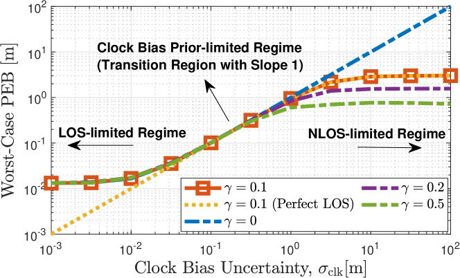
Figure 3: PEB regimes with respect to clock bias uncertainty for the digital codebook $\mathbf{F}^{\rm{digital}}$, where $\gamma$ is the reflection coefficient of the NLOS path.

IV-B Performance of Optimal and Codebook Based Strategies

In this part, we compare the worst-case PEB performances of the following signal design strategies by setting $\gamma=0.1$:

• Proposed: Optimal robust design in (17), digital and analog codebooks, $\mathbf{F}^{\rm{digital}}$ and $\mathbf{F}^{\rm{analog}}$ in (18), optimized via (22).

• Benchmark: Directional beam codebook $\mathbf{F}^{\rm{sum}}$ [8], optimized via (22) and with uniform power allocation.

Fig. 4 shows the worst-case PEBs and the relative illuminations of the LOS path for Scenario 1 and Scenario 2. Moreover, Fig. 5 illustrates the beampatterns of the considered strategies in Scenario 1 for two different values of $\sigma_{\rm{clk}}$. Finally, the average execution times on MATLAB for Scenario 1 were found to be 17.3 s (to solve (17)), 3.8 s (using $\mathbf{F}^{\rm{digital}}$ and $\mathbf{F}^{\rm{analog}}$), 3.7 s (using $\mathbf{F}^{\rm{sum}}$).

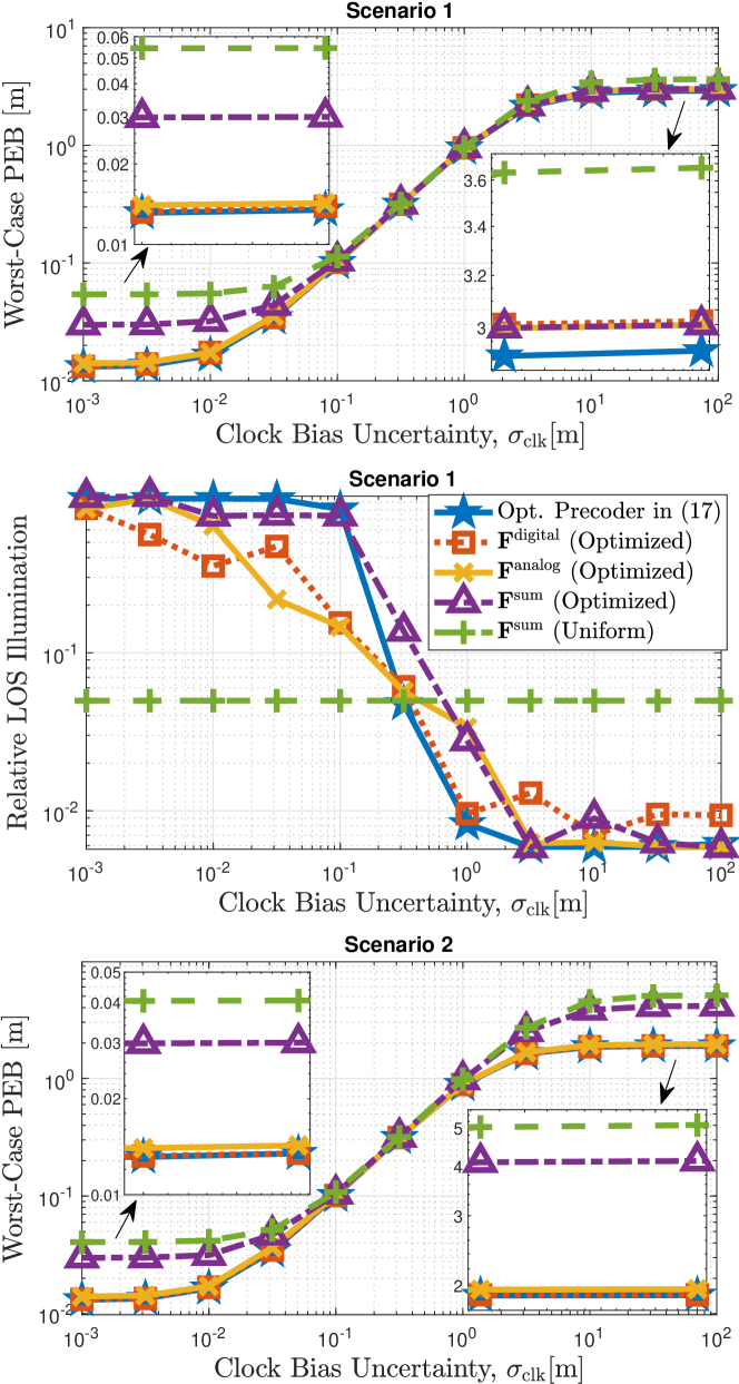
Figure 4: Worst-case PEBs and relative illuminations of the LOS path for the considered signal design strategies in Scenario 1 (large incidence location uncertainty) and Scenario 2 (small incidence location uncertainty). In Scenario 1, $N_{0}=2$ and $N_{1}=6$ beams are needed to cover the uncertainty region of the UE and the incidence point, respectively, while we have $N_{0}=N_{1}=2$ in Scenario 2. As observed from the uniform and optimized $\mathbf{F}^{\rm{sum}}$ curves, the proposed power allocation in (22) always improves positioning performance.

In agreement with the observations in Fig. 3, all strategies experience the three different PEB regimes with respect to $\sigma_{\rm{clk}}$. As expected, most of the power budget is allocated to illuminate the LOS path in the LOS-limited regime, whereas the NLOS path gets more power as $\sigma_{\rm{clk}}$ increases. Additionally, the proposed optimal strategy in (17) achieves the best performance in all operation regimes and scenarios. In Scenario 1, the proposed codebooks $\mathbf{F}^{\rm{digital}}$ and $\mathbf{F}^{\rm{analog}}$ outperform the traditional (optimized) codebook $\mathbf{F}^{\rm{sum}}$ in the LOS-limited regime, while they achieve almost the same performance in the NLOS-limited regime. The reason is that although directional beams maximize the SNR over the specified angular region (see Fig. 5), positioning requires accurate AOD estimation, which can be enabled by a balanced combination of directional and derivative beams, as illustrated in Fig. 2. Due to the relatively small uncertainty in the LOS path compared to the NLOS path in Scenario 1, $\mathbf{F}^{\rm{digital}}$ and $\mathbf{F}^{\rm{analog}}$ can provide non-negligible performance gains over $\mathbf{F}^{\rm{sum}}$ in the LOS-limited regime, whereas $\mathbf{F}^{\rm{sum}}$ in the NLOS-limited regime can produce beampatterns very similar to those achieved by $\mathbf{F}^{\rm{digital}}$ and $\mathbf{F}^{\rm{analog}}$ over a large angular region, as seen from Fig. 5. This is also corroborated by the PEB results of Scenario 2, where $\mathbf{F}^{\rm{digital}}$ and $\mathbf{F}^{\rm{analog}}$ significantly outperform $\mathbf{F}^{\rm{sum}}$ in both LOS- and NLOS-limited regimes due to low uncertainty in UE and incidence point locations.

Comparing the proposed optimal and codebook based strategies, we see that $\mathbf{F}^{\rm{digital}}$ and $\mathbf{F}^{\rm{analog}}$ exhibit PEB performances very close to the optimal approach in (17) in most cases, which implies that the proposed codebooks with optimized power allocation provide near-optimal and low-complexity solutions to spatial signal design. In addition, for all regimes and scenarios, the performance gap between $\mathbf{F}^{\rm{digital}}$ and $\mathbf{F}^{\rm{analog}}$ is negligible, which suggests that the proposed methods can be implemented in low-cost analog mmWave architectures without any loss in positioning accuracy. To summarize the main results, Table II provides practical guidelines on which spatial signals to use under different PEB regimes.

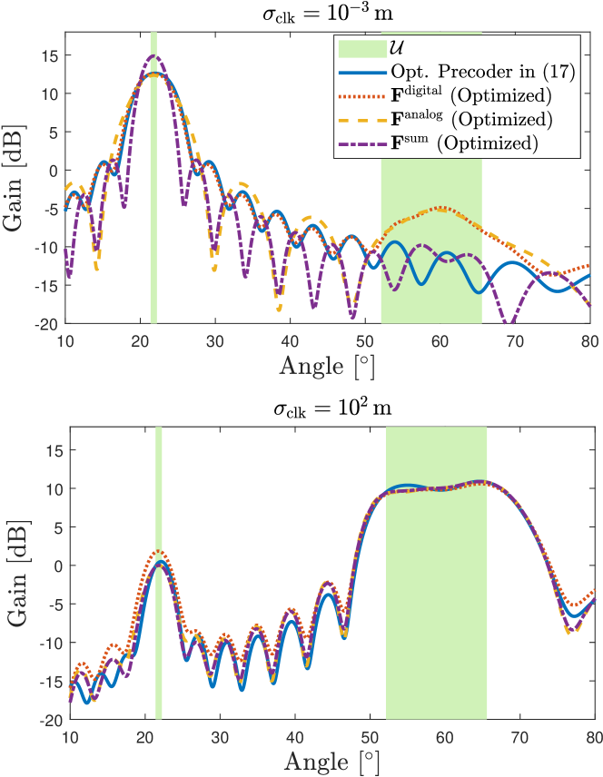
Figure 5: Aggregated beampatterns ($\left\lVert\mathbf{a}_{\rm{Tx}}^{T}(\theta)\mathbf{F}\right\rVert_{2}^{2}$) of the different strategies in Scenario 1 for two different levels of $\sigma_{\rm{clk}}$. While $\mathbf{F}^{\rm{sum}}$ maximizes the SNR towards the UE location for low $\sigma_{\rm{clk}}$, it is not positioning-optimal as the derivative beams in $\mathbf{F}^{\rm{digital}}$ and $\mathbf{F}^{\rm{analog}}$ are needed for optimality.

Table II: Guidelines on Which Spatial Signal to Use under Different PEB Regimes in Fig. 3

	LOS-limited	Clock bias prior-limited	NLOS-limited
Scenario 1	$\mathbf{F}^{\rm{analog}}$	$\mathbf{F}^{\rm{sum}}$ (Uniform)	Opt. Precoder in (17)
Scenario 2	$\mathbf{F}^{\rm{analog}}$	$\mathbf{F}^{\rm{sum}}$ (Uniform)	$\mathbf{F}^{\rm{analog}}$

IV-C Performance of Time Sharing Optimization

To validate Algorithm 1, we plot in Fig. 6 the worst-case PEBs obtained by the power allocation scheme in (22) and the time sharing scheme defined by Algorithm 1. As expected, with sufficient number of symbols per beam, time sharing can attain the same performance as power allocation since the rounding error in $L_{m}=\lfloor L\rho_{m}\rceil$ diminishes as $L$ increases.

Figure 6: Power allocation via (22) versus time sharing optimization via Algorithm 1 with respect to $L$ at $\sigma_{\rm{clk}}=10\,\rm{m}$ for $\mathbf{F}^{\rm{digital}}$ in Scenario 1.

V Conclusion

We have tackled the problem of spatial signal design for mmWave positioning under clock bias and location uncertainties. The proposed optimization-based robust design and low-complexity codebook-based heuristic designs are shown to provide significant improvements in positioning accuracy over traditional methods. Since the optimal precoder structure is valid for any scalar function of the FIM, the proposed approach can also be applied to other objectives than PEB, such as orientation error bound (OEB). Remarkably, the analog codebook can attain almost the same PEB performance as the digital one (assuming the usage of single precoding vector at the BS for each frame), which proves that high-accuracy positioning can be enabled by analog-only beamforming architectures. This result is also promising for beyond 5G systems where reconfigurable intelligent surfaces (RISs) with analog phase shifters are expected to be key enablers for positioning. As future research, we plan to investigate extensions to multi-user scenarios under multi-user or multi-BS interference constraints and frequency-dependent precoding structures (i.e., $\mathbf{f}_{m}$ will depend on the subcarrier index $k$).

Appendix A FIM Elements as a Function of $\mathbf{F}$ and $\mathbf{X}$

Assuming QPSK pilots, i.e., $\lvert s_{k,\ell}\rvert^{2}=1$, the FIM elements in (9) can be derived as follows:

$$\left[\mathbf{J}\right]_{i,j} =\frac{2}{\sigma^{2}}\sum_{k,\ell,m}\Re\left\{s_{k,\ell}^{*}\mathbf{f}_{m}^{H}\frac{\partial\mathbf{H}_{k}^{H}}{\partial\eta_{i}}\mathbf{W}\mathbf{W}^{H}\frac{\partial\mathbf{H}_{k}}{\partial\eta_{j}}\mathbf{f}_{m}s_{k,\ell}\right\}$$

$$=\frac{2}{\sigma^{2}}\sum_{k,\ell,m}\Re\left\{\lvert s_{k,\ell}\rvert^{2}{{{\rm{tr}}\left(\mathbf{f}_{m}\mathbf{f}_{m}^{H}\frac{\partial\mathbf{H}_{k}^{H}}{\partial\eta_{i}}\mathbf{W}\mathbf{W}^{H}\frac{\partial\mathbf{H}_{k}}{\partial\eta_{j}}\right)}}\right\}$$

$$=\frac{2}{\sigma^{2}}\sum_{k=0}^{K-1}\Re\left\{{{{\rm{tr}}\left(\mathbf{X}\frac{\partial\mathbf{H}_{k}^{H}}{\partial\eta_{i}}\mathbf{W}\mathbf{W}^{H}\frac{\partial\mathbf{H}_{k}}{\partial\eta_{j}}\right)}}\right\}\leavevmode\nobreak\ ,$$ (23)

where $\mathbf{X}\triangleq{\color[rgb]{0,0,0}L}\mathbf{F}\mathbf{F}^{H}={\color[rgb]{0,0,0}L}\sum_{m=0}^{M-1}\mathbf{f}_{m}\mathbf{f}_{m}^{H}$. It follows from (23) that the channel domain FIM $\mathbf{J}$ in (9) and the position domain FIM $\widetilde{\mathbf{J}}$ in (10) are functions of $\mathbf{F}$ and $\mathbf{X}$.

Appendix B Proof of Proposition 1

First, we observe from the structure of $\mathbf{J}$ in (9) that the dependence of $\mathbf{J}$ on $\mathbf{X}$ is only through the following matrices:

$$\mathbf{A}^{T}_{{\rm{Tx}}}\mathbf{X}\mathbf{A}^{*}_{{\rm{Tx}}},\leavevmode\nobreak\ \accentset{\mbox{\large.}}{\mathbf{A}}_{{{\rm{Tx}}}}^{T}\mathbf{X}\mathbf{A}^{*}_{{\rm{Tx}}},\leavevmode\nobreak\ \accentset{\mbox{\large.}}{\mathbf{A}}_{{{\rm{Tx}}}}^{T}\mathbf{X}\accentset{\mbox{\large.}}{\mathbf{A}}_{{{\rm{Tx}}}}^{*}\leavevmode\nobreak\ .$$ (24)

Following the arguments in [9, Appendix C], it can then be shown that the columns of the precoder $\mathbf{F}$ corresponding to the optimal $\mathbf{X}^{\star}=\mathbf{F}\mathbf{F}^{H}$ of (13) belong to the subspace spanned by the columns of $\mathbf{U}_{{\rm{Tx}}}$, i.e., $\bm{\Pi}^{\perp}_{\mathbf{U}_{{\rm{Tx}}}}\mathbf{F}=0$, where $\bm{\Pi}^{\perp}_{\mathbf{U}_{{\rm{Tx}}}}={\bm{\mathrm{I}}}-\bm{\Pi}_{\mathbf{U}_{{\rm{Tx}}}}$ and $\bm{\Pi}_{\mathbf{U}_{{\rm{Tx}}}}=\mathbf{U}_{{\rm{Tx}}}(\mathbf{U}_{{\rm{Tx}}}^{H}\mathbf{U}_{{\rm{Tx}}})^{-1}\mathbf{U}_{{\rm{Tx}}}^{H}$. Then, the optimal precoder covariance matrix can be expressed as

$$\mathbf{X}^{\star}=\bm{\Pi}_{\mathbf{U}_{{\rm{Tx}}}}\mathbf{F}\mathbf{F}^{H}\bm{\Pi}_{\mathbf{U}_{{\rm{Tx}}}}=\mathbf{U}_{{\rm{Tx}}}\mathbf{\Lambda}\mathbf{U}_{{\rm{Tx}}}^{H}$$ (25)

where $\mathbf{\Lambda}=(\mathbf{U}_{{\rm{Tx}}}^{H}\mathbf{U}_{{\rm{Tx}}})^{-1}\mathbf{U}_{{\rm{Tx}}}^{H}\mathbf{F}\mathbf{F}^{H}\mathbf{U}_{{\rm{Tx}}}(\mathbf{U}_{{\rm{Tx}}}^{H}\mathbf{U}_{{\rm{Tx}}})^{-1}$. ∎

References

- [1] 3rd Generation Partnership Project (3GPP), “Study on NR positioning support TR 38.855,” Technical Specification Group Radio Access Network, 2019.
- [2] R. Mendrzik et al., “Enabling situational awareness in millimeter wave massive MIMO systems,” IEEE Journal of Selected Topics in Signal Processing, vol. 13, no. 5, pp. 1196–1211, 2019.
- [3] 3rd Generation Partnership Project (3GPP), “Physical channels and modulation TS 38.211,” Technical Specification Group Radio Access Network, 2020.
- [4] J. C. Aviles et al., “Position-aided mm-wave beam training under NLOS conditions,” IEEE Access, vol. 4, pp. 8703–8714, 2016.
- [5] S. Dwivedi et al., “Positioning in 5G networks,” arXiv preprint arXiv:2102.03361, 2021.
- [6] N. Garcia et al., “Optimal precoders for tracking the AoD and AoA of a mmWave path,” IEEE Transactions on Signal Processing, vol. 66, no. 21, pp. 5718–5729, Nov 2018.
- [7] B. Zhou et al., “Successive localization and beamforming in 5G mmwave MIMO communication systems,” IEEE Transactions on Signal Processing, vol. 67, no. 6, pp. 1620–1635, 2019.
- [8] A. Kakkavas et al., “Power allocation and parameter estimation for multipath-based 5G positioning,” IEEE Transactions on Wireless Communications, pp. 1–1, 2021.
- [9] J. Li et al., “Range compression and waveform optimization for MIMO radar: A Cramér–Rao bound based study,” IEEE Transactions on Signal Processing, vol. 56, no. 1, pp. 218–232, 2007.
- [10] U. Nickel, “Overview of generalized monopulse estimation,” IEEE Aerospace and Electronic Systems Magazine, vol. 21, no. 6, pp. 27–56, 2006.
- [11] A. Shahmansoori et al., “Position and orientation estimation through millimeter-wave MIMO in 5G systems,” IEEE Transactions on Wireless Communications, vol. 17, no. 3, pp. 1822–1835, 2017.
- [12] A. Kakkavas et al., “Performance limits of single-anchor millimeter-wave positioning,” IEEE Transactions on Wireless Communications, vol. 18, no. 11, pp. 5196–5210, 2019.
- [13] S. M. Kay, Fundamentals of Statistical Signal Processing: Practical Algorithm Development. Pearson Education, 2013, vol. 3.
- [14] S. Boyd et al., Convex Optimization. Cambridge university press, 2004.
- [15] Z.-Q. Luo et al., “Semidefinite relaxation of quadratic optimization problems,” IEEE Signal Processing Magazine, vol. 27, no. 3, pp. 20–34, 2010.
- [16] O. El Ayach et al., “Spatially sparse precoding in millimeter wave MIMO systems,” IEEE Transactions on Wireless Communications, vol. 13, no. 3, pp. 1499–1513, 2014.
- [17] M. Grant et al., “CVX: Matlab software for disciplined convex programming, version 2.1,” http://cvxr.com/cvx, Mar. 2014.
- [18] J. A. Zhang et al., “Multibeam for joint communication and radar sensing using steerable analog antenna arrays,” IEEE Transactions on Vehicular Technology, vol. 68, no. 1, pp. 671–685, 2018.
- [19] S. J. Orfanidis, Electromagnetic waves and antennas. Rutgers University New Brunswick, NJ, 2002.
- [20] J. Tranter et al., “Fast unit-modulus least squares with applications in beamforming,” IEEE Transactions on Signal Processing, vol. 65, no. 11, pp. 2875–2887, 2017.
- [21] A. Nemirovski, “Interior point polynomial time methods in convex programming,” Lecture notes, 2004.
- [22] Y. Han et al., “Performance limits and geometric properties of array localization,” IEEE Transactions on Information Theory, vol. 62, no. 2, pp. 1054–1075, 2016.
- [23] 3rd Generation Partnership Project (3GPP), “Study on NR positioning enhancements TR 38.857,” Technical Specification Group Radio Access Network, 2021.