Summing Up Smart Transitions

Abstract

Some of the most significant high-level properties of currencies are the sums of certain account balances. Properties of such sums can ensure the integrity of currencies and transactions. For example, the sum of balances should not be changed by a transfer operation. Currencies manipulated by code present a verification challenge to mathematically prove their integrity by reasoning about computer programs that operate over them, e.g., in Solidity. The ability to reason about sums is essential: even the simplest ERC-20 token standard of the Ethereum community provides a way to access the total supply of balances.

Unfortunately, reasoning about code written against this interface is non-trivial: the number of addresses is unbounded, and establishing global invariants like the preservation of the sum of the balances by operations like transfer requires higher-order reasoning. In particular, automated reasoners do not provide ways to specify summations of arbitrary length.

In this paper, we present a generalization of first-order logic which can express the unbounded sum of balances. We prove the decidablity of one of our extensions and the undecidability of a slightly richer one. We introduce first-order encodings to automate reasoning over software transitions with summations. We demonstrate the applicability of our results by using SMT solvers and first-order provers for validating the correctness of common transitions in smart contracts.

This submission is an extended version of the CAV 2021 paper ”Summing Up Smart Transitions”, by N. Elad, S. Rain, N. Immerman, L. Kovács and M. Sagiv.

1 Introduction

A basic challenge in smart contract verification is how to express the functional correctness of transactions, such as currency minting or transferring between accounts. Typically, the correctness of such a transaction can be verified by proving that the transaction leaves the sum of certain account balances unchanged.

Consider for example the task of minting an unbounded number of tokens in the simplified ERC-20 token standard of the Ethereum community [31], as illustrated in Figure 1. This example deposits the minted amount (n) into the receiver’s address (a) and we need to ensure that the mint operation only changed the balance of the receiver. To do so, in addition to (i) proving that the balance of the receiver has been increased by n, we also need to verify that (ii) the account balance of every user address a^′ different than a has not been changed during the mint operation and that (iii) the sum of all balances changed exactly by the amount that was minted. The validity of these three requirements (i)-(iii), formulated as the post-conditions of Figure 1, imply its functional correctness.

⬇

a: Address

ingrulemint(a,n) \listingrule# Post-conditions assert new-bal(a) = old-bal(a) + n\hfill#(i) for each Address a$’$$\neq$a:\hfill#(ii) assert new-bal(a$’$) = old-bal(a$’$) assert new-sum() = old-sum() + n\hfill␣#(iii)’

Figure 1: Minting $n$ Tokens in ERC-20.

Surprisingly, proving formulas similar to the post-conditions of Figure 1 is challenging for state-of-the-art automated reasoners, such as SMT solvers [7, 6, 9] and first-order provers [18, 10, 33]: it requires reasoning that links local changes of the receiver (a) with a global state capturing the sum of all balances, as well as constructing that global state as an aggregate of an unbounded but finite number of Address balances. Moreover, our encoding of the problem uses discrete coins that are minted and deposited, whose number is unbounded but finite as well.

In this paper we address verification challenges of software transactions with aggregate properties, such as preservation of sums by transitions that manipulate low-level, individual entities. Such properties are best expressed in higher-order logic, hindering the use of existing automated reasoners for proving them. To overcome such a reasoning limitation, we introduce Sum Logic (SL) as a generalization of first-order logic, in particular of Presburger arithmetic. Previous works [20, 30, 11] have also introduced extensions of first-order logic with aggregates by counting quantifiers or generalized quantifiers. In Sum Logic (SL) we only consider the special case of integer sums over uninterpreted functions, allowing us to formalize SL properties with and about unbounded sums, in particular sums of account balances, without higher-order operations (Section 3). We prove the decidability of one of our SL extensions and the undecidability of a slightly richer one (Section 4). Given previous results [20], our undecidability result is not surprising. In contrast, what may be unexpected is our decidability result and the fact that we can use our first-order fragment for a convenient and practical new way to verify the correctness of smart contracts.

We further introduce first-order encodings which enable automated reasoning over software transactions with summations in SL (Section 5). Unlike [5], where SMT-specific extensions supporting higher-order reasoning have been introduced, the logical encodings we propose allow one to use existing reasoners without any modification. We are not restricted to SMT reasoning, but can also leverage generic automated reasoners, such as first-order theorem provers, supporting first-order logic. We believe our results ease applying automated reasoning to smart contract verification even for non-experts.

We demonstrate the practical applicability of our results by using SMT solvers and first-order provers for validating the correctness of common financial transitions appearing in smart contracts (Section 6). We refer to these transitions as smart transitions. We encode SL into pure first-order logic by adding another sort that represents the tokens of the crypto-currency themselves (which we dub “coins”).

Although the encodings of Section 5 do not translate to our decidable SL fragment from Section 4, our experimental results show that automated reasoning engines can handle them consistently and fast. The decidability results of Section 5 set the boundaries for what one can expect to achieve, while our experiments from Section 5 demonstrate that the unknown middle-ground can still be automated.

While our work is mainly motivated by smart contract verification, our results can be used for arbitrary software transactions implementing sum/aggregate properties. Further, when compared to the smart contract verification framework of [32], we note that we are not restricted to proving the correctness of smart contracts as finite-state machines, but can deal with semantic properties expressing financial transactions in smart contracts, such as currency minting/transfers.

While ghost variable approaches [13] can reason about changes to the global state (the sum), our approach allows the verifier to specify only the local changes and automatically prove the impact on the global state.

Contributions.

In summary, this paper makes the following contributions:

• We present a generalization to Presburger arithmetic (SL, in Section 3) that allows expressing properties about summations. We show how we can formalize verification problems of smart contracts in SL.

• We discuss the decidability problem of checking validity of SL formulas (Section 4): we prove that it is undecidable in the general case, but also that there exists a small decidable fragment.

• We show different encodings of SL to first-order logic (Section 5). To this end, we consider theory-specific reasoning and variations of SL, for example by replacing non-negative integer reasoning with term algebra properties.

• We evaluate our results with SMT solvers and first-order theorem provers, by using 31 new benchmarks encoding smart transitions and their properties (Section 6). Our experiments demonstrate the applicability of our results within automated reasoning, in a fully automated manner, without any user guidance.

2 Preliminaries

We consider many-sorted first-order logic (FOL) with equality, defined in the standard way. The equality symbol is denoted by $\approx$.

We denote by $\text{STRUCT}\left[\Sigma\right]$ the set of all structures for the vocabulary $\Sigma$. A structure $\mathcal{A}\in\text{STRUCT}\left[\Sigma\right]$ is a pair $\left(\mathcal{D},\mathcal{I}\right)$, where for each sort $\boldsymbol{s}$, its domain in $\mathcal{A}$ is $\mathcal{D}(\boldsymbol{s})$, and for each symbol $S$, its interpretation in $\mathcal{A}$ is $\mathcal{I}(S)$. Note that models of a formula $\varphi$ over a vocabulary $\Sigma$ are structures $\mathcal{A}\in\text{STRUCT}\left[\Sigma\right]$.

A first-order theory is a set of first-order formulas closed under logical consequence. We will consider, the first-order theory of the natural numbers with addition. This is Presburger arithmetic (PA) which is of course decidable [26].
We write $\mathbb{N}$ to denote the set of natural numbers. We consider $0\in\mathbb{N}$ and write $\mathbb{N}^{+}$ to explicitly exclude $0$ from $\mathbb{N}$. The vocabulary of PA is $\Sigma_{\text{Presburger}}=\left(0,1,c_{1},\dots,c_{l},+^{2}\right)$, with all constants $0,1,c_{i}$ of sort Nat. A structure $\mathcal{A}=(\mathcal{D},\mathcal{I})\in\text{STRUCT}\left[\Sigma_{\text{Presburger}}\right]$ is called a Standard Model of Arithmetic when $\mathcal{D}(\textnormal{{Nat}})=\mathbb{N}$ and $+^{2}$ is interpreted as the standard binary addition $+$ function over the naturals. The vocabulary $\Sigma_{\text{Presburger}}$ can be extended with a total order relation, yielding $\Sigma^{*}_{\text{Presburger}}=\left(0,1,+^{2},\leq^{2}\right)$, where $\leq^{2}$ is interpreted as the binary relation $\leq$ in Standard Models of Arithmetic.

3 Sum Logic (SL)

We now define Sum Logic (SL) as a generalization of Presburger arithmetic, extending Presburger arithmetic with unbounded sums. SL is motivated by applications of financial transactions over cryptocurrencies in smart contracts. Smart contracts are decentralized computer programs executed on a blockchain-based system, as explained in [27]. Among other tasks, they automate financial transactions such as transferring and minting money. We refer to these transactions as smart transitions. The aim of this paper and SL in particular is to express and reason about the post-conditions of smart transitions similar to Figure 1.

SL expresses smart transition relations among sums of accounts of various kinds, e.g., at different banks, times, etc. Each such kind, $j$, is modeled by an uninterpreted function symbol, $b_{j}$, where $b_{j}(a)$ denotes the balance of $a$’s account of kind $j$, and a constant symbol $s_{j}$, which denotes the sum of all outputs of $b_{j}$. As such, our SL generalizes Presburger arithmetic with (i) a sort Address corresponding to the (unbounded) set of account addresses; (ii) balance functions $b_{j}$ mapping account addresses from Address to account values of sort Nat; and (iii) sum constants $s_{j}$ of sort Nat capturing the total sum of all account balances represented by $b_{j}$. Formally, the vocabulary of SL is defined as follows.

Definition 1 (SL Vocabulary)

Let

$$\Sigma^{l,m,d}_{+,\leq}=\left(a_{1},\dots,a_{l},b^{1}_{1},\dots,b^{1}_{m},c_{1},\dots,c_{d},s_{1},\dots,s_{m},0,1,+^{2},\leq^{2}\right)$$

be a sorted first-order vocabulary of SL over sorts $\left\{\textnormal{{Address}},\textnormal{{Nat}}\right\}$, where

• (Addresses) The constants $a_{1},\dots,a_{l}$ are of sort Address;

• (Balance functions) $b^{1}_{1},\dots,b^{1}_{m}$ are unary function symbols from Address to Nat;

• (Constants and Sums) The constants $c_{1},\dots,c_{d},s_{1},\dots,s_{m}$ and $0,1$ are of sort Nat;

• $+^{2}$ is a binary function $\textnormal{{Nat}}\times\textnormal{{Nat}}\to\textnormal{{Nat}}$;

• $\leq^{2}$ is a binary relation over $\textnormal{{Nat}}\times\textnormal{{Nat}}$.

In what follows, when the cardinalities in an SL vocabulary are clear from context, we simply write $\Sigma$ instead of $\Sigma^{l,m,d}_{+,\leq}$. Further, by $\Sigma^{l,m,d}_{\cancel{+},\cancel{\leq}}$ we denote the sub-vocabulary where the crossed-out symbols are not available. Note that even when addition is not available, we still allow writing numerals larger than 1.

We restrict ourselves to universal sentences over an SL vocabulary, with quantification only over the Address sort.

We now extend the Tarskian semantics of first-order logic to ensure that the sum constants of an SL vocabulary ($s_{1},\dots,s_{m}$) are equal to the sum of outputs of their associated balance functions ($b_{j}$ for each $s_{j}$) over the respective entire domains of sort Address.

Let $\Sigma$ be an SL vocabulary. An SL structure $\mathcal{A}=\left(\mathcal{D},\mathcal{I}\right)\in\text{STRUCT}\left[\Sigma\right]$ representing a model for an SL formula $\varphi$ is called an SL model iff

$$\mathcal{I}(s_{j})=\sum_{a\in\mathcal{D}(\textnormal{{Address}})}\left[\mathcal{I}(b_{j})\right](a),\quad\text{for each }1\leq j\leq m.$$

We write $\mathcal{A}\vDash_{{\textsc{SL}}{}}\varphi$ to mean that $\mathcal{A}$ is an SL model of $\varphi$. When it is clear from context, we simply write $\mathcal{A}\vDash\varphi$.

Function	Encoding in SL	Reference in ERC-20
sum	$s$ or $s^{\prime}$	totalSupply
bal$(a)$	$b(a)$ or $b^{\prime}(a)$	balanceOf
mint$(a,v)$	$b^{\prime}(a)\approx b(a)+v$	transfer
transferFrom$(f,t,v)$	$b^{\prime}(t)\approx b(t)+v\land b(f)\approx b^{\prime}(f)+v$	transferFrom

Table 1: ERC-20 Token Standard

Example 1 (Encoding ERC-20 in SL)

As a use case of SL, we showcase the encoding of the ERC-20 token standard of the Ethereum community [31] in SL. To this end, we consider an SL vocabulary $\Sigma^{l,2,d}$. We respectively denote the balance functions and their associated sums as $b,b^{\prime},s,s^{\prime}$ in the SL structure over $\Sigma^{l,2,d}$. The resulting instance of SL can then be used to encode ERC-20 operations/smart transitions as SL formulas, as shown in Table 1. Using this encoding, the post-condition of Figure 1 is expressed as the SL formula

$$b^{\prime}(a)\approx b(a)+n\;\land\;\forall a^{\prime}\not\approx a.b^{\prime}(a^{\prime})\approx b(a^{\prime})\;\land\;s^{\prime}\approx s+n$$ (1)

formalizing the correctness of the smart transition of minting $n$ tokens in Figure 1. In the applied verification examples in Section 6, rather than verifying the low-level implementation of built-in functions such as $\textnormal{{mint}}_{n}$, we assume their correctness by including suitable axioms.

4 Decidability of SL

We consider the decidability problem of verifying formulas in SL. We show that when there are several function symbols $b_{j}$ to sum over, the satisfiability problem for SL becomes undecidable. We first present, however, a useful decidable fragment of SL.

4.1 A Decidable Fragment of SL

We prove decidability for a fragment of SL, which we call the $\left(l,1,d\right)$-FRAG fragment of SL (Theorem 4.4). For doing so, we reduce the fragment to Presburger arithmetic, by using regular Presburger constructs to encode SL extensions, that is the uninterpreted functions and sum constants of SL.

The first step of our reduction proof is to consider distinct models, which are models where the Address constants $a_{i}$ represent distinct elements in the domain $\mathcal{D}(\textnormal{{Address}})$. While this restriction is somewhat unnatural, we show that for each vocabulary and formula that has a model, there exists an equisatisfiable formula over a different vocabulary that has a distinct model (Theorem 4.1). The crux of our decidability proof is then proving that $\left(l,1,d\right)$-FRAG has small Address space: given a formula $\varphi$, if it is satisfiable, then there exists a model where $\left|\mathcal{D}(\textnormal{{Address}})\right|\leq\kappa(\left|\varphi\right|)$, $\left|\varphi\right|$ is the length of $\varphi$, and $\kappa(.)$ is some computable function (Theorem 4.3).

4.1.1 Distinct Models

An SL structure $\mathcal{A}$ is considered distinct when the $l$ Address constants represent $l$ distinct elements in $\mathcal{D}(\textnormal{{Address}})$. I.e.,

$$\left|\left\{\mathcal{I}(a_{1}),\dots,\mathcal{I}(a_{l})\right\}\right|=l\,.$$

Since each SL model induces an equivalence relation over the Address constants, we consider partitions $P$ over $\left\{a_{1},\dots,a_{l}\right\}$. For each possible partition $P$ we define a transformation of terms and formulas $\mathcal{T}_{P}$ that substitutes equivalent Address constants with a single Address constant. The resulting formulas are defined over a vocabulary that has $\left|P\right|$ Address constants. We show that given an SL formula $\varphi$, if $\varphi$ has a model, we can always find a partition $P$ such that each of its classes corresponds to an equivalence class induced by that model.

Theorem 4.1 (Distinct Models)

Let $\varphi$ be an SL formula over $\Sigma$, then $\varphi$ has a model iff there exists a partition $P$ of $\left\{a_{1},\dots,a_{l}\right\}$ such that $\mathcal{T}_{P}(\varphi)$ has a distinct model.∎

4.1.2 Small Address Space

In order to construct a reduction to Presburger arithmetic, we bound the size of the Address sort. For a fragment of SL to be decidable, we therefore need a way to bound its models upfront. We formalize this requirement as follows.

Definition 2 (Small Address Space)

Let FRAG be some fragment of SL over vocabulary $\Sigma=\Sigma^{l,m,d}_{+,\leq}$. FRAG is said to have small Address space if there exists a computable function $\kappa_{\Sigma}(.)$, such that for any SL formula $\varphi\in\textsc{FRAG}$, $\varphi$ has a distinct model iff $\varphi$ has a distinct model $\mathcal{A}=(\mathcal{D},\mathcal{I})$ with small Address space, where $\left|\mathcal{D}(\textnormal{{Address}})\right|\leq\kappa_{\Sigma}(\left|\varphi\right|)$.

We call $\kappa_{\Sigma}(.)$ the bound function of FRAG; when the vocabulary is clear from context we simply write $\kappa(.)$.

One instance of a fragment (or rather, family of fragments) that satisfies this property is the $\left(l,1,d\right)$-FRAG fragment: the simple case of a single uninterpreted “balance” function (and its associated sum constant), further restricted by removing the binary function $+$ and the binary relation $\leq$. Therefore, we derive the following theorem:

Theorem 4.2 (Small Address Space of $\left(l,1,d\right)$-FRAG)

For any $l$, $d$, it holds $\left(l,1,d\right)$-FRAG, the fragment of SL formulas over the SL vocabulary

$$\Sigma^{l,1,d}_{\cancel{+},\cancel{\leq}}=\left(a_{1},\dots,a_{l},b^{1},c_{1},\dots,c_{d},s,0,1\right)\;,$$

has small Address space with bound function $\kappa(x)=l+x+1$.∎

An attempt to trivially extend Theorem 4.2 for a fragment of SL with two balance functions falls apart in a few places, but most importantly when comparing balances to the sum of a different balance function. In Section 4.2 we show that these comparisons are essential for proving our undecidability result in SL.

4.1.3 Presburger Reduction

For showing decidability of some FRAG fragment of SL, we describe a Turing reduction to pure Presburger arithmetic. We introduce a transformation $\tau(.)$ of formulas in SL into formulas in Presburger arithmetic. It maps universal quantifiers to disjunctions, and sums to explicit addition of all balances. In addition, we define an auxiliary formula $\eta(\varphi)$, which ensures only valid addresses are considered, and that invalid addresses have zero balances. The formal definitions of $\tau(.)$ and $\eta(\varphi)$ can be found in Appendix 0.A.

By relying on the properties of distinctness and small Address space we get the following results.

Theorem 4.3 (Presburger Reduction)

An SL formula $\varphi$ has a distinct, SL model with small Address space iff $\tau(\varphi)\land\eta(\varphi)$ has a Standard Model of Arithmetic.∎

Theorem 4.4 (SL Decidability)

Let FRAG be a fragment of SL that has small Address space, as defined in Definition 2. Then, FRAG is decidable.

Proof (Theorem 4.4)

Let $\varphi$ be a formula in FRAG. Then $\varphi$ has an SL model iff for some partition $P$ of $\left\{a_{1},\dots,a_{l}\right\}$, $\mathcal{T}_{P}(\varphi)$ has a distinct SL model. For any $P$, the formula $\mathcal{T}_{P}(\varphi)$ is in FRAG, therefore $\mathcal{T}_{P}(\varphi)$ has a distinct SL model iff it has a distinct SL model with small Address space.

From Theorem 4.3, we get that for any $P$, $\varphi_{P}\triangleq\mathcal{T}_{P}(\varphi)$ has a distinct SL model iff $\tau(\varphi_{P})\land\eta(\varphi_{P})$ has a Standard Model of Arithmetic. By using the PA decision procedure as an oracle, we obtain the following decision procedure for a FRAG formula $\varphi$:

• For each possible partition $P$ of $\left\{a_{1},\dots,a_{l}\right\}$, let $\varphi_{P}=\mathcal{T}_{P}(\varphi)$;

• Using a PA decision procedure, check whether $\tau(\varphi_{P})\land\eta(\varphi_{P})$ has a model, for each $P$;

• If a model for some partition $P$ was found, the formula $\varphi_{P}$ has a distinct SL model, and therefore $\varphi$ has SL model;

• Otherwise, there is no distinct SL model for any partition $P$, and therefore there is no SL model for $\varphi$.

Remark 1

Our decision procedure for Theorem 4.4 requires $B_{l}$ Presburger queries, where $B_{l}$ is Bell’s number for all possible partitions of a set of size $l$.

Using Theorem 4.4 and Theorem 4.2, we then obtain the following result.

Corollary 1

$\left(l,1,d\right)$-FRAG is decidable.∎

4.2 SL Undecidability

We now show that simple extensions of our decidable $\left(l,1,d\right)$-FRAG fragment lose its decidability (Theorem 4.5). For doing so, we encode the halting problem of a two-counter machine using SL with 3 balance functions, thereby proving that the resulting SL fragment is undecidable.

Consider a two-counter machine, whose transitions are encoded by the Presburger formula $\pi(c_{1},c_{2},p,c^{\prime}_{1},c^{\prime}_{2},p^{\prime})$ with 6 free variables: 2 for each of the three registers, one of which being the program counter (pc). We assume w.l.o.g. that all three registers are within $\mathbb{N}^{+}$, allowing us to use addresses with a zero balance as a special “separator”. In addition, we assume that the program counter is 1 at the start of the execution, and that there exists a single halting statement at line $H$. That is, the two-counter machine halts iff the pc is equal to $H$.

	Address	$l(\textnormal{{Address}})$	$c(\textnormal{{Address}})$	$g(\textnormal{{Address}})$
{4*[Time-step #0]		0	1	0
		1	1	$c_{1}$ at #0
		2	1	$c_{2}$ at #0
	$a_{0}$	3	1	pc at #0 = 1
	⋮	⋮	⋮	⋮
{4*[Time-step #$i$]	$x_{1}$	$4i$	1	0
	$x_{2}$	$4i+1$	1	$c_{1}$ at #$i$
	$x_{3}$	$4i+2$	1	$c_{2}$ at #$i$
	$x_{4}$	$4i+3$	1	pc at #$i$
{4*[Time-step #$(i+1)$]	$x_{5}$	$4i+4$	1	0
	$x_{6}$	$4i+5$	1	$c_{1}$ at #$(i+1)$
	$x_{7}$	$4i+6$	1	$c_{2}$ at #$(i+1)$
	$x_{8}$	$4i+7$	1	pc at #$(i+1)$
	⋮	⋮	⋮	⋮
{4*[Time-step #$n=\frac{s_{c}}{4}-1$]		$s_{c}-4$	1	0
		$s_{c}-3$	1	$c_{1}$ at #$n$
		$s_{c}-2$	1	$c_{2}$ at #$n$
	$a_{1}$	$s_{c}-1$	1	pc at #$n$ = $H$

Table 2: Transition System of a 2-Counter Machine, Array View.

4.2.1 Reduction Setting

We have 4 Address elements for each time-step, 3 of them hold one register each, and one is used to separate between each group of Address elements (see Table 2). We have 3 uninterpreted functions from Address to Nat (“balances”). For readability we denote these functions as $c,l,g$ (instead of $b_{1},b_{2},b_{3}$) and their respective sums as $s_{c},s_{l},s_{g}$:

1. Function $c\,$: Cardinality function, used to force size constraints. We set its value for all addresses to be $1$, and therefore the number of addresses is $s_{c}$.

2. Function $l\,$: Labeling function, to order the time-steps. We choose one element to have a maximal value of $s_{c}-1$ and ensure that $l$ is injective. This means that the values of $l$ are distinctly $[0,s_{c}-1]$.

3. Function $g\,$: General purpose function, which holds either one of the registers or 0 to mark the Address element as a separating one.

Each group representing a time-step is a 4 Address element, ordered as follows:

1. First, a separating Address element $x$ (where $g(x)$ is 0).

2. Then, the two general-purpose counters.

3. Lastly, the program counter.

In addition we have 2 Address constants, $a_{0}$ and $a_{1}$ which represent the pc value at the start and at the end of the execution. The element $a_{1}$ also holds the maximal value of $l$, that is, $l(a_{1})+1\approx s_{c}$. Further, $a_{0}$ holds the fourth-minimal value, since its the last element of the first group, and each group has four elements.

4.2.2 Formalization Using a Two-Counter Machine

We now formalize our reduction, proving undecidability of SL.

(i) We impose an injective labeling

$$\varphi_{1}=\forall x,y.\left(l(x)\approx l(y)\right)\to\left(x\approx y\right)$$

(ii) We next formalize properties over the program counter pc. The Address constant that represents the program counter pc value of the last time-step is set to have the maximal labeling, that is

$$\varphi_{2}=\forall x.l(x)\leq l(a_{1})$$

Further, the Address constant that represents the pc value of the first time-step has the fourth labeling, hence

$$\varphi_{3}=l(a_{0})\approx 3$$

Finally, the first and last values of the program counter are respectively 1 and $H$, that is

$$\varphi_{4}=g(a_{0})\approx 1\land g(a_{1})\approx H$$

(iii) We express cardinality constraints ensuring that there are as many Address elements as the labeling of the last Address constant ($a_{1}$) + 1. We assert

$$\varphi_{5}=\left(s_{c}\approx l(a_{1})+1\right)\land\forall x.\left(c(x)\approx 1\right)$$

(iv) We encode the transitions of the two-counter machine, as follows. For every 8 Address elements, if they represent two sequential time-steps, then the formula for the transitions of the two-counter machine is valid for the registers it holds. As such, we have

$$\varphi_{6}=\forall x_{1},\dots,x_{8}.\left(F1\land F2\land F3\right)$$

$$\to\pi\left(g(x_{2}),g(x_{3}),g(x_{4}),g(x_{6}),g(x_{7}),g(x_{8})\right)$$

where the conjunction $F1\land F2\land F3$ expresses that $x_{1},\dots,x_{8}$ are two sequential time-steps, with $F1$, $F2$ and $F3$ defined as below. In particular, $F1$, $F2$ and $F3$ formalize that $x_{1},\dots,x_{8}$ have sequential labeling, starting with one zero-valued Address element (“separator”) and continuing with 3 non-zero elements, as follows:

• Sequential:

  $$l(x_{2})\approx l(x_{1})+1\land\dots\land l(x_{8})\approx l(x_{7})+1$$

• Time-steps:

  $$g(x_{1})\approx 0\land g(x_{2})>0\land g(x_{3})>0\land g(x_{4})>0\;,$$ (F2)

  $$g(x_{5})\approx 0\land g(x_{6})>0\land g(x_{7})>0\land g(x_{8})>0$$ (F3)

Based on the above formalization, the formula $\varphi=\varphi_{1}\land\dots\land\varphi_{6}$ is satisfiable iff the two-counter machine halts within a finite amount of time-steps (and the exact amount would be given by $\frac{s_{c}}{4}$). Since the halting problem for two-counter machines is undecidable, our SL, already with 3 uninterpreted functions and their associated sums, is also undecidable.

Theorem 4.5

For any $l\geq 2,m\geq 3$ and $d$, any fragment of SL over $\Sigma^{l,m,d}_{+,\leq}$ is undecidable. ∎

Remark 2

Note that in the above formalization the only use of associated sums comes from expressing the size of the set of Address elements. As for our uninterpreted function $c(.)$ we have $\forall x.c(x)\approx 1$, its sum $s_{c}$ is thus the amount of addresses. Hence, we can encode the halting problem for two-counter machines in an almost identical way to the encoding presented here, using a generalization of PA with two uninterpreted functions for $l(.)$ and $g(.)$, and a size operation replacing $c(.)$ and its associated sum.

5 SL Encodings of Smart Transitions

The definition of SL models in Sections 3 and 4 ensured that the summation constants $s_{j}$ were respectively equal to the actual summation of all balances $b_{j}(.)$. In this section, we address the challenge to formalize relations between $s_{j}$ and $b_{j}(.)$ in a way that the resulting encodings can be expressed in the logical frameworks of automated reasoners, in particular of SMT solvers and first-order theorem provers.

In what follows, we consider a single transaction or one time-step of multiple transactions over $s_{j},b_{j}(.)$. We refer to such transitions as smart transitions. Smart transitions are common in smart contracts, expressing for example the minting and/or transferring of some coins, as evidenced in Figure 1 and discussed later.

Based on Section 3, our smart transitions are encoded in the $\Sigma^{l,2,d}$ fragment of SL. Note however, that neither decidability nor undecidability of this fragment is implied by Theorem 4.4, nor Theorem 4.5. In this section, we show that our SL encoding of smart transitions is expressible in first-order logic. We first introduce a sound, implicit SL encoding, by “hiding” away sum semantics and using invariant relations over smart transitions (Section 5.1). This encoding does not allow us to directly assert the values of any balance or sum, but we can prove that this implicit encoding is complete, relative to a translation function (Section 5.2).

By further restricting our implicit SL encoding to this relative complete setting, we consider counting properties to explicitly reason with balances and directly express verification conditions with unbounded sums on $s_{j}$ and $b_{j}(.)$. This is shown in Section 5.3, and we evaluate different variants of the explicit SL encoding in Section 6, showcasing their practical use and relevance within automated reasoning.

To directly present our SL encodings and results in the smart contract domain, in what follows we rely on the notation of Table 1. As such, we respectively denote $b,b^{\prime}$ by old-bal, new-bal and write old-sum, new-sum for $s,s^{\prime}$. As already discussed in Figure 1, the prefixes old- and new- refer to the entire state expressed in the encoding before and after the smart transition. We explicitly indicate this state using old-world, new-world respectively. The non-prefixed versions bal and sum are stand-ins for both the old- and new- versions — Figure 2 illustrates our setting for the smart transition of minting one coin.

With this SL notation at hand, we are thus interested in finding first-order formulas that verify smart transition relations between old-sum and new-sum, given the relation between old-bal and new-bal. In this paper, we mainly focus on the smart transitions of minting and transferring money, yet our results could be used in the context of other financial transactions/software transitions over unbounded sums.

Example 2

In the case of minting $n$ coins in Figure 1, we require formulas that (a) describe the state before the transition (the old-world, thus pre-condition), (b) formalize the transition (the relation between old-bal and new-bal; (i)-(ii) in Figure 1) and (c) imply the consequences for the new-world ((iii) in Figure 1). These formulas verify that minting and depositing $n$ coins into some address result in an increase of the sum by $n$, that is $\textnormal{{new-}}\textnormal{{sum}}=\textnormal{{old-}}\textnormal{{sum}}+n$, as expressed in the functional correctness formula (1) of Figure 1.

5.1 SL Encoding using Implicit Balances and Sums

The first encoding we present is a set of first-order formulas with equality over sorts $\left\{\textnormal{{Coin}},\,\textnormal{{Address}}\right\}$. No additional theories are considered. The Coin sort represents money, where one coin is one unit of money. The Address sort represents the account addresses as before. As a consequence, balance functions and sum constants only exist implicitly in this encoding. As such, the property $\textnormal{{sum}}=\sum_{a\in\textnormal{{Address}}}\textnormal{{bal}}(a)$ cannot be directly expressed in this encoding. Instead, we formalize this property by using so-called smart invariant relations between two predicates has-coin and active over coins $c\in\textnormal{{Coin}}$ and $a\in\textnormal{{Address}}$, as follows.

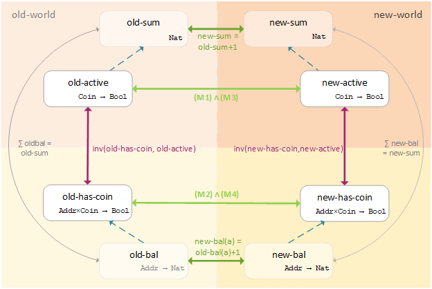
Figure 2: Implicit SL Encoding of $\textnormal{{mint}}_{1}$, where Addr is short for Address.

Definition 3 (Smart Invariants)

Let $\textnormal{{has-coin}}\subseteq\textnormal{{Address}}{}\times\textnormal{{Coin}}{}$ and consider $\textnormal{{active}}\subseteq\textnormal{{Coin}}{}$. A smart invariant of the pair $\left(\textnormal{{has-coin}},\,\textnormal{{active}}\right)\,$ is the conjunction of the following three formulas

1. Only active coins $c$ can be owned by an address $a$:

   $$\forall c:\textnormal{{Coin}}.\;\exists a:\textnormal{{Address}}.\;\textnormal{{has-coin}}(a,c)\to\textnormal{{active}}(c)\;.$$

2. Every active coin $c$ belongs to some address $a$:

   $$\forall c:\textnormal{{Coin}}.\;\textnormal{{active}}(c)\to\exists a:\textnormal{{Address}}.\;\textnormal{{has-coin}}(a,c)\;.$$

3. Every coin $c$ belongs to at most one address $a$:

   $$\forall c:\textnormal{{Coin}}. \forall a,a^{\prime}:\textnormal{{Address}}.$$ (I3)

   $$\left(\textnormal{{has-coin}}(a,c)\land\textnormal{{has-coin}}(a^{\prime},c)\to a\approx a^{\prime}\right).$$

We write $\textnormal{{inv}}(\textnormal{{has-coin}}{},\;\textnormal{{active}}{})$ to denote the smart invariant $\text{(I1)}\land\text{(I2)}\land\text{(I3)}$ of $\left(\textnormal{{has-coin}},\,\textnormal{{active}}\right)\,$.

Intuitively, our smart invariants ensure that a coin $c$ is active iff it is owned by precisely one address $a$. Our smart invariants imply the soundness of our implicit SL encoding, as follows.

Theorem 5.1 (Soundness of SL Encoding)

Given that $\textnormal{{sum}}=\left|\textnormal{{active}}\right|$ and for every $a\in\textnormal{{Address}}$ it holds $\textnormal{{bal}}(a)=\left|\left\{c\in\textnormal{{Coin}}\mid\left(a,c\right)\in\textnormal{{has-coin}}\right\}\right|$, then $\textnormal{{inv}}(\textnormal{{has-coin}},\textnormal{{active}})\;\Longrightarrow\;\textnormal{{sum}}=\sum_{a\in\textnormal{{Address}}}\textnormal{{bal}}(a)$. ∎

We say that a smart transition preserves smart invariants, when

inv $$(\textnormal{{old-}}\textnormal{{has-coin}},\textnormal{{old-}}\textnormal{{active}})$$

$$\iff\textnormal{{inv}}(\textnormal{{new-}}\textnormal{{has-coin}},\textnormal{{new-}}\textnormal{{active}}),$$

where $\textnormal{{old-}}\textnormal{{has-coin}},\textnormal{{old-}}\textnormal{{active}}$ and $\textnormal{{new-}}\textnormal{{has-coin}},\textnormal{{new-}}\textnormal{{active}}$ respectively denote the functions $\textnormal{{has-coin}},\textnormal{{active}}$ in the states before and after the smart transition. Based on the soundness of our implicit SL encoding, we formalize smart transitions preserving smart invariants as first-order formulas. We only discuss smart transitions implementing minting $n$ coins here, but other transitions, such as transferring coins, can be handled in a similar manner. We first focus on miniting a single coin, as follows.

Definition 4 (Transition $\textnormal{{mint}}_{1}(a,c)$)

Let there be $c\in\textnormal{{Coin}},a\in\textnormal{{Address}}$. The transition $\textnormal{{mint}}_{1}(a,c)$ activates coin $c$ and deposits it into address $a$.

1. The coin $c$ was inactive before and is active now:

   $$\neg\textnormal{{old-}}\textnormal{{active}}(c)\land\textnormal{{new-}}\textnormal{{active}}(c)\;.$$

2. The address $a$ owns the new coin $c$:

   $$\textnormal{{new-}}\textnormal{{has-coin}}(a,c)\land\forall a^{\prime}:\textnormal{{Address}}{}.\;\neg\textnormal{{old-}}\textnormal{{has-coin}}(a^{\prime},c)\;.$$

3. Everything else stays the same:

   $$\forall c^{\prime}:\textnormal{{Coin}}.\;c^{\prime}\not\approx c\to\left(\textnormal{{new-}}\textnormal{{active}}(c^{\prime})\leftrightarrow\textnormal{{old-}}\textnormal{{active}}(c^{\prime})\right)\;,$$ (M3)

   $$\forall c^{\prime}:\textnormal{{Coin}}.\;\forall a^{\prime}:\textnormal{{Address}}.\;\;(c^{\prime}\not\approx c\lor a^{\prime}\not\approx a)\to$$ (M4)

   $$\qquad\left(\textnormal{{new-}}\textnormal{{has-coin}}(a^{\prime},c^{\prime})\leftrightarrow\textnormal{{old-}}\textnormal{{has-coin}}(a^{\prime},c^{\prime})\right)\;.$$

The transition $\textnormal{{mint}}_{1}(a,c)$ is defined as $\text{(M1)}\land\text{(M2)}\land\text{(M3)}\land\text{(M4)}$.

By minting one coin, the balance of precisely one address, that is of the receiver’s address, increases by one, whereas all other balances remain unchanged. Thus, the expected impact on the sum of account balances is also increased by one, as illustrated in Figure 2. The following theorem proves that the definition of $\textnormal{{mint}}_{1}$ is sound. That is, $\textnormal{{mint}}_{1}$ affects the implicit balances and sums as expected and hence $\textnormal{{mint}}_{1}$ preserves smart invariants.

Theorem 5.2 (Soundness of $\textnormal{{mint}}_{1}(a,c)$)

Let $c\in\textnormal{{Coin}}$, $a\in\textnormal{{Address}}$ such that $\textnormal{{mint}}_{1}(a,c)$. Consider balance functions old-bal, $\textnormal{{new-}}\textnormal{{bal}}:\textnormal{{Address}}\to\mathbb{N}$, non-negative integer constants old-sum, new-sum, unary predicates old-active, $\textnormal{{new-}}\textnormal{{active}}\subseteq\textnormal{{Coin}}$ and binary predicates old-has-coin, $\textnormal{{new-}}\textnormal{{has-coin}}\subseteq\textnormal{{Address}}\times\textnormal{{Coin}}$ such that

$$\left|\textnormal{{old-}}\textnormal{{active}}\right|=\textnormal{{old-}}\textnormal{{sum}}\,,\;\left|\textnormal{{new-}}\textnormal{{active}}\right|=\textnormal{{new-}}\textnormal{{sum}},$$

and for every address $a^{\prime}$, we have

$$\textnormal{{old-}}\textnormal{{bal}}(a^{\prime})=\left|\left\{c^{\prime}\in\textnormal{{Coin}}\mid(a^{\prime},c^{\prime})\in\textnormal{{old-}}\textnormal{{has-coin}}\right\}\right|\,,$$

$$\textnormal{{new-}}\textnormal{{bal}}(a^{\prime})=\left|\left\{c^{\prime}\in\textnormal{{Coin}}\mid(a^{\prime},c^{\prime})\in\textnormal{{new-}}\textnormal{{has-coin}}\right\}\right|\;.$$

Then, $\textnormal{{new-}}\textnormal{{sum}}=\textnormal{{old-}}\textnormal{{sum}}+1$, $\textnormal{{new-}}\textnormal{{bal}}(a)=\textnormal{{old-}}\textnormal{{bal}}(a)+1$. Moreover, for all other addresses $a^{\prime}\neq a$, it holds $\textnormal{{new-}}\textnormal{{bal}}(a^{\prime})=\textnormal{{old-}}\textnormal{{bal}}(a^{\prime})$. ∎

Smart transitions minting an arbitrary number of $n$ coins, as in our  Figure 1, is then realized by repeating the $\textnormal{{mint}}_{1}$ transition $n$ times. Based on the soundness of $\textnormal{{mint}}_{1}$, ensuring that $\textnormal{{mint}}_{1}$ preserves smart invariants, we conclude by induction that $n$ repetitions of $\textnormal{{mint}}_{1}$, that is minting $n$ coins, also preserves smart invariants. The precise definition of $\textnormal{{mint}}_{n}$ together with the soundness result is stated in Section 0.B.2.

5.2 Completeness Relative to a Translation Function

Smart invariants provide sufficient conditions for ensuring soundness of our SL encodings (Theorem 5.1). We next show that, under additional constraints, smart invariants are also necessary conditions, establishing thus (relative) completeness of our encodings.

A straightforward extension of Theorem 5.1 however does not hold. Namely, only under the assumptions of Theorem 5.1, the following formula is not valid:

$$\textnormal{{sum}}=\sum_{a\in\textnormal{{Address}}}\textnormal{{bal}}(a)\quad\iff\quad\textnormal{{inv}}(\textnormal{{has-coin}}{},\;\textnormal{{active}}{})\,.$$

As a counterexample, assume (i) $\textnormal{{sum}}=\left|\textnormal{{active}}\right|$, (ii) for every $a\in\textnormal{{Address}}$ it holds that $\textnormal{{bal}}(a)=\left|\left\{c\in\textnormal{{Coin}}\mid(a,c)\in\textnormal{{has-coin}}\right\}\right|$, that is the assumptions of Theorem 5.1. Further, let (iii) the smart invariants inv(has-coin, active) hold for all but the coins $c_{1},c_{2}\in\textnormal{{Coin}}$ and all but the addresses $a_{1},a_{2}\in\textnormal{{Address}}$. We also assume that (iv) $c_{1}$ is active but not owned by any address and (v) $c_{2}$ is active and owned by the two distinct addresses $a_{1},a_{2}$. We thus have $\textnormal{{sum}}=\sum_{a\in\textnormal{{Address}}}\textnormal{{bal}}(a)$, yet $\textnormal{{inv}}(\textnormal{{has-coin}}{},\;\textnormal{{active}}{})$ does not hold.

To ensure completeness of our encodings, we therefore introduce a translation function $f$ that restricts the set $\mathcal{F}\triangleq 2^{\textnormal{{Address}}\times\textnormal{{Coin}}}\times 2^{\textnormal{{Coin}}}$ of $(\textnormal{{has-coin}},\textnormal{{active}})$ pairs, as follows. We exclude from $\mathcal{F}$ those pairs $(\textnormal{{has-coin}},\textnormal{{active}})$ that violate smart invariants by both (i) not satisfying (I2), as (I2) ensures that there are not too many active coins, and by (ii) not satisfying at least one of (I1) and (I3), as (I1) and (I3) ensure that there are not too few active coins. The required translation function $f$ (Section 0.B.3) now assigns every pair $(\textnormal{{bal}},\textnormal{{sum}})$ the set of all $(\textnormal{{has-coin}},\textnormal{{active}})\in\mathcal{F}$ that satisfy $\textnormal{{sum}}=\left|\textnormal{{active}}\right|$, $\textnormal{{bal}}(a)=\left|\left\{c\in\textnormal{{Coin}}\mid\textnormal{{has-coin}}(a,c)\right\}\right|$ for every address $a$ and have not been excluded.

Theorem 5.3 (Relative Completeness of SL Encoding)

Let $(\textnormal{{bal}},\textnormal{{sum}})\in\mathbb{N}^{\textnormal{{Address}}}\times\mathbb{N}$ and let $(\textnormal{{has-coin}},\textnormal{{active}})\in f(\textnormal{{bal}},\textnormal{{sum}})$ be arbitrary. Then,

$$\textnormal{{sum}}=\sum_{a\in\textnormal{{Address}}}\textnormal{{bal}}(a)\quad\iff\quad\textnormal{{inv}}\,(\textnormal{{has-coin}}{},\;\textnormal{{active}}{})\;.\qquad\squareforqed$$

5.3 SL Encodings using Explicit Balances and Sums

We now restrict our SL encoding from Section 5.1 to explicitly reason with balance functions during smart transitions. We do so by expressing our translation function $f$ from Section 5.2 in first-order logic. We now use the summation constant $\textnormal{{sum}}\in\mathbb{N}$ and the balance function $\textnormal{{bal}}:\textnormal{{Address}}\to\mathbb{N}$ in our SL encoding. In particular, we use our smart invariants $\textnormal{{inv}}(\textnormal{{has-coin}}{},\;\textnormal{{active}}{})$ in this explicit SL encoding together with two additional axioms (Ax1, Ax2), ensuring that $\textnormal{{sum}}=\left|\textnormal{{active}}\right|$ and $\textnormal{{bal}}(a)=\left|\left\{c\in\textnormal{{Coin}}\mid\textnormal{{has-coin}}(a,c)\right\}\right|$ for all $a\in\textnormal{{Address}}$.

To formalize the additional properties, we introduce two counting mechanisms in our SL encoding. The first one is a bijective function $\textnormal{{count}}:\textnormal{{Coin}}\to\mathbb{N}^{+}$ and the second one is a function $\textnormal{{idx}}:\textnormal{{Address}}\times\textnormal{{Coin}}\to\mathbb{N}^{+}$, where $\textnormal{{idx}}(a,.):\textnormal{{Coin}}\to\mathbb{N}^{+}$ is bijective for every $a\in\textnormal{{Address}}$. To ensure that count and $\textnormal{{idx}}(a,.)$ count coins, we impose the following two properties:

$$\forall c:\textnormal{{Coin}}.\;\textnormal{{active}}(c)\iff\textnormal{{count}}(c)\leq\textnormal{{sum}}\;,$$

$$\forall c:\textnormal{{Coin}}.\;\forall a:\textnormal{{Address}}.\;\textnormal{{has-coin}}(a,c)\iff\textnormal{{idx}}(a,c)\leq\textnormal{{bal}}(a)\;.$$

Figure 3 illustrates our revised SL encoding for our smart transition $\textnormal{{mint}}_{1}$. We next ensure soundness of our resulting explicit encoding for summation, as follows.

Theorem 5.4 (Soundness of Explicit SL Encodings)

Let there be a pair $(\textnormal{{bal}},\textnormal{{sum}})\in\mathbb{N}^{\textnormal{{Address}}}\times\mathbb{N}$, a pair $(\textnormal{{has-coin}},\textnormal{{active}})\in\mathcal{F}$, and functions $\textnormal{{count}}:\textnormal{{Coin}}{}\to\mathbb{N}^{+}$ and $\textnormal{{idx}}:\textnormal{{Address}}\times\textnormal{{Coin}}\to\mathbb{N}^{+}$.

Given that count is bijective, $\textnormal{{idx}}(a,.):\textnormal{{Coin}}\to\mathbb{N}^{+}$ is bijective for every $a\in\textnormal{{Address}}$, and that (Ax1), (Ax2) and $\textnormal{{inv}}\,(\textnormal{{has-coin}}{},\;\textnormal{{active}}{})$ hold, then, $\textnormal{{sum}}=\left|\textnormal{{active}}\right|$ and $\textnormal{{bal}}(a)=\left|\left\{c\in\textnormal{{Coin}}{}:\textnormal{{has-coin}}(a,c)\right\}\right|$, for every $a\in\textnormal{{Address}}$.

In particular, we have $\textnormal{{sum}}=\sum_{a\in\textnormal{{Address}}}\textnormal{{bal}}(a)$.∎

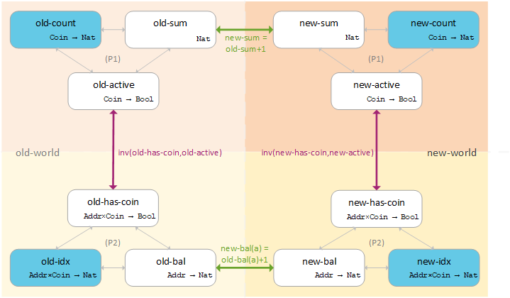
Figure 3: Explicit SL Encoding of $\textnormal{{mint}}_{1}$, where Addr is short for Address.

When compared to Section 5.1, our explicit SL encoding introduced above uses our smart invariants as axioms of our encoding, together with (Ax1) and (Ax2). In our explicit SL encoding, the post-conditions asserting functional correctness of smart transitions express thus relations among old-sum to new-sum. For example, for $\textnormal{{mint}}_{n}$ we are interested in ensuring

$$\textnormal{{mint}}_{n}\Rightarrow\textnormal{{new-}}\textnormal{{sum}}=\textnormal{{old-}}\textnormal{{sum}}+n\;.$$ (2)

By using two new constants old-total, $\texttt{new-total}\in\mathbb{N}$, we can use $\textnormal{{sum}}=\texttt{total}$ as smart invariant for $\textnormal{{mint}}_{n}$. As a result, the property to be ensured is then

$$\begin{array}[]{l}(\textnormal{{old-}}\textnormal{{sum}}=\texttt{old-total}\land\texttt{new-total}=\texttt{old-total}+n\land\textnormal{{mint}}_{n})\\ \Rightarrow\left(\textnormal{{new-}}\textnormal{{sum}}=\texttt{new-total}\right)\;.\end{array}$$ (3)

It is easy to see that the negations of (2) and (3) are equisatisfiable. We note however that the additional constants old-total, new-total used in (3) lead to unstable results within automated reasoners, as discussed in Section 6.

6 Experiments

From Theory to Practice. To make our explicit SL encodings handier for automated reasoners, we improved the setting illustrated in Figure 3 by applying the following restrictions without losing any generality.

(i) The predicates has-coin and active were removed from the explicit SL encodings, by replacing them by their equivalent expressions (Ax1)-(Ax2).

(ii) The surjectivity assertions of count and idx were restricted to the relevant intervals $[1,\textnormal{{sum}}]$, $[1,\textnormal{{bal}}(a)]$ respectively.

(iii) Compared to Figure 3, only one mutual count and one mutual idx functions were used. We however conclude that we do not lose expressivity of our resulting SL encoding, as shown in Section 0.B.5.

(iv) When our SL encoding contains expressions such as $\forall c:\textnormal{{Coin}}.\;\textnormal{{idx}}(a_{0},c)\in[l_{0},u_{0}]\iff\textnormal{{idx}}(a_{1},c)\in[l_{1},u_{1}]$, with $a_{0}$, $a_{1}$ being distinct addresses such that either $u_{i}\leq\textnormal{{bal}}(a_{i})$ or $l_{i}>\textnormal{{bal}}(a_{i})$, $i\in\left\{0,1\right\}$, then it can be assumed that the coins in those intervals are in the same order for both functions (Section 0.B.6).

Based on the above, we derive three different explicit SL encodings to be used in automated reasoning about smart transitions. We respectively denote these explicit SL encodings by int, nat and id, and describe them next.

Benchmarks. In our experiments, we consider four smart transitions $\textnormal{{mint}}_{1}$, $\textnormal{{mint}}_{n}$, $\textnormal{{transferFrom}}_{1}$ and $\textnormal{{transferFrom}}_{n}$, respectively denoting minting and transferring one and $n$ coins. These transitions capture the main operations of linear integer arithmetic. In particular, $\textnormal{{mint}}_{n}$ implements the smart transition of our running example from Figure 1.

For each of the four smart transitions, we implement four SL encodings: the implicit SL encoding uf from Section 5.1 using only uninterpreted functions and three explicit encodings int, nat and id as variants of Section 5.3. We also consider three additional arithmetic benchmarks using int, which are not directly motivated by smart contracts. Together with variants of int and nat presented in the sequel, our benchmark set contains 31 examples altogether, with each example being formalized in the SMT-LIB input syntax [1]. In addition to our encodings, we also proved consistency of the axioms used in our encodings.

SL Encodings and Relaxations. Our explicit SL encoding int uses linear integer arithmetic, whereas nat and id are based on natural numbers. As naturals are not a built-in theory in SMT-LIB, we assert the axioms of Presburger arithmetic directly in the encodings of nat and id.

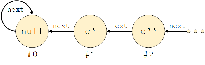
Figure 4: Linked Lists in id.

In our id encodings, inductive datatypes are additionally used to order coins. There exists one linked list of all coins for count and one for each $\textnormal{{idx}}(a,.)$, $a\in\textnormal{{Address}}$. Additionally, there exists a “null” coin, which is the first element of every list and is not owned by any address. As shown in Figure 4, the numbering of each coin is defined by its position in the respective list. This way surjectivity for count and idx can respectively be asserted by the formulas $\exists c:\textnormal{{Coin}}.\;\textnormal{{count}}(c)\approx\textnormal{{sum}}$ and $\forall a:\textnormal{{Address}}.\;\exists c:\textnormal{{Coin}}.\;\textnormal{{idx}}(a,c)\approx\textnormal{{bal}}(a)$. However, asserting surjectivity for int and nat cannot be achieved without quantifying over $\mathbb{N}^{+}$. Such quantification would drastically effect the performance of automated reasoners in (fragments of) first-order logics. As a remedy, within the default encodings of int and nat, we only consider relevant instances of surjectivity.

Further, we consider variations of int and nat by asserting proper surjectivity to the relevant intervals of idx and count (denoted as surj) and/or adding the total constants mentioned in Section 5.3 (denoted as with total, no total) . These variations of int and nat are implemented for $\textnormal{{mint}}_{1}$ and $\textnormal{{transferFrom}}_{1}$.

Experimental Setting. We evaluated our benchmark set of 31 examples using SMT solvers Z3 [7] and CVC4 [6], as well as the first-order theorem prover Vampire [18]. Our experiments were run on a standard machine with an Intel Core i5-6200U CPU (2.30GHz, 2.40GHz) and 8 GB RAM. The time is given in seconds and we ran all experiments with a time limit of 300s. Time out is indicated by the symbol $\times$. The default parameters were used for each solver, unless stated otherwise in the corresponding tables. The precise calls of the solvers, together with examples of the encodings, can be found in Appendix 0.C.

$\textnormal{{mint}}_{1}$				$\textnormal{{transferFrom}}_{1}$
no total	Z3	CVC4	Vampire	no total	Z3	CVC4	Vampire
nat	0.02	$\times$	0.92	nat	$\times$	$\times$	15.35
nat surj.	$\times$	$\times$	$\times$	nat surj.	100.03	$\times$	$\times$
int	0.02	0.03	$\times$	int	0.02	0.07	$\times$
int surj.	$\times$	5.96	$\times$	int surj.	1.02	$\times$	$\times$
with total	Z3	CVC4	Vampire	with total	Z3	CVC4	Vampire
nat	0.03	$\times$	2.92	nat	0.28	$\times$	22.54
nat surj.	0.11	$\times$	$\times$	nat surj.	38.24	$\times$	$\times$
int	0.02	0.03	$\times$	int	0.02	0.10	$\times$
int surj.	3.81	5.95	$\times$	int surj.	$\times$	6.56	$\times$

Table 3: Results of $\textnormal{{mint}}_{1}$ and $\texttt{transferFrom}_{1}$ using nat and int, with/without the total Constants and with/without Surjectivity.

Experimental Analysis. We first report on our experiments using different variations of int and nat. Table 3 shows that asserting complete surjectivity for int and nat is computationally hard and indeed significantly effects the performance of automated reasoners. Thus, for the following experiments only relevant instances of surjectivity, such as $\exists c:\textnormal{{Coin}}.\,\textnormal{{count}}(c)=\textnormal{{sum}}$ were asserted in int and nat. Table 3 also illustrates the instability of using the total constant. Some tasks seem to be easier even though their reasoning difficulty increased strictly by adding additional constants.

Encoding	Task
	$\textnormal{{mint}}_{1}$		$\textnormal{{transferFrom}}_{1}$		$\textnormal{{mint}}_{n}$		$\textnormal{{transferFrom}}_{n}$
uf	Z3: CVC4: Vampire:	0.01 0.02 0.18	Z3: CVC4: Vampire:	0.02 0.03 0.19	Z3: CVC4: Vampire:	$\times$ $\times$ $0.35^{*}$	Z3: CVC4: Vampire:	$\times$ $\times$ $0.44^{*}$
nat	Z3: CVC4: Vampire:	0.02 $\times$ 0.92	Z3: CVC4: Vampire:	$\times$ $\times$ 15.35	Z3: CVC4: Vampire:	$\times$ $\times$ $23.23^{\dagger}$	Z3: CVC4: Vampire:	$\times$ $\times$ $228.22^{\dagger}$
int	Z3: CVC4: Vampire:	0.02 0.03 $\times$	Z3: CVC4: Vampire:	0.02 0.07 $\times$	Z3: CVC4: Vampire:	0.03 0.05 $\times$	Z3: CVC4: Vampire:	0.11 0.35 $\times$
id	Z3: CVC4: Vampire:	$\times$ $\times$ $7.36^{\ddagger}$	Z3: CVC4: Vampire:	$\times$ $\times$ $17.16^{\ddagger}$	Z3: CVC4: Vampire:	$\times$ $\times$ $23.52^{\ddagger}$	Z3: CVC4: Vampire:	$\times$ $\times$ $\times$

Table 4: Smart Transitions using Implicit/Explicit SL Encodings.

Our most important experimental findings are shown in Table 4, demonstrating that our SL encodings are suitable for automated reasoners. Thanks to our explicit SL encodings, each solver can certify every smart transition in at least one encoding. Our explicit SL encodings are more relevant than the implicit encoding uf as we can express and compare any two non-negative integer sums, whereas for uf handling arbitrary values $n$ can only be done by iterating over the $\textnormal{{mint}}_{1}$ (or $\textnormal{{transferFrom}}_{1}$) transition. This iteration requires inductive reasoning, which currently only Vampire could do [14], as indicated by the superscript $*$. Nevertheless, the transactions $\textnormal{{mint}}_{1}$, $\textnormal{{transferFrom}}_{1}$, which involve only one coin in uf, require no inductive reasoning as the actual sum is not considered; each of our solvers can certify these examples.

We note that the tasks $\textnormal{{mint}}_{n}$ and $\textnormal{{transferFrom}}_{n}$ from Table 4 yield a huge search space when using their explicit SL encodings within automated reasoners. We split these tasks into proving intermediate lemmas and proved each of these lemmas independently, by the respective solver. In particular, we used one lemma for $\textnormal{{mint}}_{n}$ and four lemmas for $\textnormal{{transferFrom}}_{n}$. In our experiments, we only used the recent theory reasoning framework of Vampire with split queues [12] and indicate our results in by superscript $\dagger$.

We further remark that our explicit SL encoding id using inductive datatypes also requires inductive reasoning about smart transitions and beyond. The need of induction explains why SMT solvers failed proving our id benchmarks, as shown in Table 4. We note that Vampire found a proof using built-in induction [14] and theory-specific reasoning [12], as indicated by superscript $\ddagger$.

We conclude by showing the generality of our approach beyond smart transitions. It in fact enables fully automated reasoning about any two summations $\sum_{i\in I}g(i)$, $\sum_{i\in I}h(i)$ of non-negative integer values $g(i)$, $h(i)$ ($i\in I$) over a mutual finite set $I$. The examples of Table 5 affirm this claim.

Task		Time
Transition	Impact
$\textnormal{{new-}}\textnormal{{bal}}(a_{0})=\textnormal{{old-}}\textnormal{{bal}}(a_{0})+3$ $\textnormal{{new-}}\textnormal{{bal}}(a_{1})=\textnormal{{old-}}\textnormal{{bal}}(a_{1})-3$	$\textnormal{{new-}}\textnormal{{sum}}=\textnormal{{old-}}\textnormal{{sum}}$	Z3: CVC4: Vampire:	0.20 1.28 $\times$
$\textnormal{{new-}}\textnormal{{bal}}(a_{0})=\textnormal{{old-}}\textnormal{{bal}}(a_{0})+4$ $\textnormal{{new-}}\textnormal{{bal}}(a_{1})=\textnormal{{old-}}\textnormal{{bal}}(a_{1})-2$	$\textnormal{{new-}}\textnormal{{sum}}=\textnormal{{old-}}\textnormal{{sum}}+2$	Z3: CVC4: Vampire:	0.58 7.14 $\times$
$\textnormal{{new-}}\textnormal{{bal}}(a_{0})=\textnormal{{old-}}\textnormal{{bal}}(a_{0})+5$ $\textnormal{{new-}}\textnormal{{bal}}(a_{1})=\textnormal{{old-}}\textnormal{{bal}}(a_{1})-3$ $\textnormal{{new-}}\textnormal{{bal}}(a_{2})=\textnormal{{old-}}\textnormal{{bal}}(a_{2})-1$	$\textnormal{{new-}}\textnormal{{sum}}=\textnormal{{old-}}\textnormal{{sum}}+1$	Z3: CVC4: Vampire:	1.52 155.20 $\times$

Table 5: Arithmetic Reasoning in the Explicit SL Encoding int.

7 Related work

Smart Contract Safety. Formal verification of smart contracts is an emerging hot topic because of the value of the assets stored in smart contracts, e.g. the DeFi software [3]. Due to the nature of the blockchain, bugs in smart contracts are irreversible and thus the demand for provably bug-free smart contracts is high.

The K interactive framework has been used to verify safety of a smart contract, e.g. in [22]. Isabelle [21] was also shown to be useful in manual, interactive verification of smart contracts [16]. We, however, focus on automated approaches.

There are also efforts to perform deductive verification of smart contracts both on the source level in languages such as Solidity [32, 4, 13] and Move [34], as well as on the the Ethereum virtual machine (EVM) level [2, 28]. This paper improves the effectiveness of these approaches by developing techniques for automatically reasoning about unbounded sums. This way, we believe we support a more semantic-based verification of smart contracts.

Our approach differs from works using ghost variables [13], since we do not manually update the “ghost state”. Instead, the verifier needs only to reason about the local changes, and the aggregate state is maintained by the axioms. That means other approaches assume (a) the local changes and (b) the impact on ghost variables (sum), whereas we only assume (a) and automatically prove $a\Rightarrow b$. This way, we reduce the user-guidance in providing and proving (b).

Our work complements approaches that verify smart contracts as finite state machines [32] and methods, like ZEUS [17], using symbolic model checking and abstract interpretation to verify generic safety properties for smart contracts.

The work in [29] provides an extensive evaluation of ERC-20 and ERC-721 tokens. ERC-721 extends ERC-20 with ownership functions, one of which being “approve”. It enables transactions on another party’s behalf. This is independent of our ability to express sums in first-order logic, as the transaction’s initiator is irrelevant to its effect.

Reasoning about Financial Applications. Recently, the Imandra prover introduced an automated reasoning framework for financial applications [23, 24, 25]. Similarly to our approach, these works use SMT procedures to verify and/or generate counter-examples to safety properties of low- and high-level algorithms. In particular, results of [23, 24, 25] include examples of verifying ranking orders in matching logics of exchanges, proving high-level properties such as transitivity and anti-symmetry of such orders. In contrast, we focus on verifying properties relating local changes in balances to changes of the global state (the sum). Moreover, our encodings enable automated reasoning both in SMT solving and first-order theorem proving.

Automated Aggregate Reasoning. The theory of first-order logic with aggregate operators has been thoroughly studied in [15, 20]. Though proven to be strictly more expressive than first-order logic, both in the case of general aggregates as well as simple counting logics, in this paper we present a practical way to encode a weakened version of aggregates (specifically sums) in first-order logic. Our encoding (as in Section 5) works by expressing particular sums of interest, harnessing domain knowledge to avoid the need of general aggregate operators.

Previous works [19, 5] in the field of higher-order reasoning do not directly discuss aggregates. The work of [19] extends Presburger arithmetic with Boolean algebra for finite, unbounded sets of uninterpreted elements. This includes a way to express the set cardinalities and to compare them against integer variables, but does not support uninterpreted functions, such as the balance functions we use throughout our approach.

The SMT-based framework of [5] takes a different, white-box approach, modifying the inner workings of SMT solvers to support higher-order logic. We on the other hand treat theorem provers and SMT solvers as black-boxes, constructing first-order formulas that are tailored to their capabilities. This allows us to use any off-the-shelf SMT solver.

In [8], an SMT module for the theory of FO(Agg) is presented, which can be used in all DPLL-based SAT, SMT and ASP solvers. However, FO(Agg) only provides a way to express functions that have sets or similar constructs as inputs, but not to verify their semantic behavior.

8 Conclusions

We present a methodology for reasoning about unbounded sums in the context of smart transitions, that is transitions that occur in smart contracts modeling transactions. Our sum logic SL and its usage of sum constants, instead of fully-fledged sum operators, turns out to be most appropriate for the setting of smart contracts. We show that SL has decidable fragments (Section 4.1), as well as undecidable ones (Section 4.2). Using two phases to first implicitly encode SL in first-order logic (Section 5.1), and then explicitly encode it (Section 5.3), allows us to use off-the-shelf automated reasoners in new ways, and automatically verify the semantic correctness of smart transitions.

Showing the (un)decidability of the SL fragment with two sets of uninterpreted functions and sums is an interesting step for further work, as this fragment supports encoding smart transition systems. Another interesting direction of future work is to apply our approach to different aggregates, such as minimum and maximum and to reason about under which conditions these values stay above/below certain thresholds. A slightly modified setting of our SL axioms can already handle $\min$/$\max$ aggregates in a basic way, namely by using $\geq$ and $\leq$ instead of equality and dropping the injectivity/surjectivity (respectively) axioms of the counting mechanisms.

Summing upon multidimensional arrays in various ways is yet another direction of future research. Our approach supports the summation over all values in all dimensions by adding the required number of parameters to the predicate idx and by adapting the axioms accordingly.

Appendix 0.A Proofs for Sum Logic

Definition 5 (SL Structure)

Let $\Sigma$ be an SL vocabulary. We write a structure $\mathcal{A}=(\mathcal{D},\mathcal{I})\in\text{STRUCT}\left[\Sigma\right]$ as a tuple

$$\mathcal{A}=\left(A,\mathbb{N},a^{\mathcal{A}}_{1},\dots,a^{\mathcal{A}}_{l},b^{\mathcal{A}}_{1},\dots,b^{\mathcal{A}}_{m},c^{\mathcal{A}}_{1},\dots,c^{\mathcal{A}}_{d},s^{\mathcal{A}}_{1},\dots,s^{\mathcal{A}}_{m},0,1,+,\leq\right)$$

where $A=\mathcal{D}(\textnormal{{Address}})$ is some finite , possibly empty set. We have $a_{i}^{\mathcal{A}}=\mathcal{I}(a_{i})\in A$; $b^{\mathcal{A}}_{j}=\mathcal{I}(b^{1}_{j})\in\mathbb{N}^{A}$; and $c_{k}^{\mathcal{A}}=\mathcal{I}(c_{k}),s^{\mathcal{A}}_{j}=\mathcal{I}(s_{j})\in\mathbb{N}$.

We always assume that $\mathcal{D}(\textnormal{{Nat}})=\mathbb{N}$, and that $0,1,+^{2}$ and $\leq^{2}$ are interpreted naturally. For brevity, we omit them when describing SL structures.

Distinct Models Proof

Observation 1

For any set $X$ and any partition $P$ thereof, it holds that $\left|P\right|\leq\left|X\right|$.

Definition 6 (Partition-Induced Function)

Let $P$ be a partition of a finite set $X$ of size $l$. $P=\left\{A_{1},\dots,A_{l^{\prime}}\right\}$ where $l^{\prime}\leq l$.

We define the partition-induced function $f_{P}(x)$ (for any $x\in X$) as the index $i$ such that $A_{i}\in P$ and $x\in A_{i}$.

For brevity, we denote $f_{P}(x)$ as $P(x)$.

Definition 7 (Function-Induced Equivalence Class)

Let $f$ be some function over some set $X$. We define the function-induced equivalence class for each $x\in X$ as

$$[x]_{f}\triangleq\left\{x^{\prime}\in X\mid f(x^{\prime})=f(x)\right\}.$$

Definition 8 (Function-Induced Partition)

Let $f$ be some function defined over some set $X$. We define the function-induced partition $P_{f}$ as

$$P_{f}\triangleq\left\{[x]_{f}\mid x\in X\right\}.$$

Definition 9 (Partitioning Sum Terms by $P$)

Let $t$ be some term over an SL vocabulary $\Sigma=\Sigma^{l,m,d}$ (with $l$ Address constants) and let $P$ be some partition of $\left\{a_{1},\dots,a_{l}\right\}$.

We define a transformation $\mathcal{T}_{P}(t)$ inductively as a term over an SL vocabulary $\Sigma_{P}=\Sigma^{l^{\prime},m,d}$ with $l^{\prime}=\left|P\right|\leq l$ Address constants:

$$\mathcal{T}_{P}(t)\triangleq\left\{\begin{array}[]{ll}a_{P(a_{i})}&\mbox{if }t=a_{i}\\ x_{i}&\mbox{if }t=x_{i}\text{ of sort }\textnormal{{Address}}\\ s_{j}&\mbox{if }t=s_{j}\\ b_{j}(\mathcal{T}_{P}(t_{1}))&\mbox{if }t=b_{j}(t_{1})\text{ where $t_{1}$ is some $a_{i}$ or $x_{i}$}\\ \mathcal{T}_{P}(t_{1})+\mathcal{T}_{P}(t_{2})&\mbox{if }t=t_{1}+t_{2}\end{array}\right.$$

Definition 10 (Partitioning an SL Formula by $P$)

We naturally extend the terms transformation $\mathcal{T}_{P}$ to formulas.

Observation 2

For any SL vocabulary $\Sigma$, $\Sigma_{P}\subseteq\Sigma$, since $l^{\prime}\leq l$. Therefore, for any formula $\varphi$ in some fragment FRAG of SL, $\mathcal{T}_{P}(\varphi)\in\text{FRAG}$ as well.

Definition 11 (Distinct Structures)

An SL structure $\mathcal{A}$ is considered distinct when $\left|\left\{a_{1}^{\mathcal{A}},\dots,a_{l}^{\mathcal{A}}\right\}\right|=l$. I.e. the $l$ Address constants represent $l$ distinct elements in $\mathcal{D}(\textnormal{{Address}})$.

See 4.1 Proof of Theorem 4.1

Part 1: If $\varphi$ has an SL model, then there exists some partition $P$ such that $\mathcal{T}_{P}(\varphi)$ has a distinct SL model ($\Rightarrow$)

Let $\mathcal{A}$ be some SL model of $\varphi$ and let $f$ be the mapping from $\left\{a_{1},\dots,a_{l}\right\}$ to $A$, i.e

$$f(a_{i})\triangleq a_{i}^{\mathcal{A}}$$

Let $P$ be the partition (of size $l^{\prime}$) induced by $f$ and we construct a distinct SL model

$$A^{\prime}=\left(A,a^{\prime}_{1},\dots,a^{\prime}_{l^{\prime}},b_{1}^{\mathcal{A}},\dots,b_{m}^{\mathcal{A}},c_{1}^{\mathcal{A}},\dots,c_{n}^{\mathcal{A}},s_{1}^{\mathcal{A}},\dots,s_{m}^{\mathcal{A}}\right)$$

for $\mathcal{T}_{P}(\varphi)$, where $A$, $b_{1}^{\mathcal{A}},\dots,b_{m}^{\mathcal{A}}$, $c_{1}^{\mathcal{A}},\dots,c_{n}^{\mathcal{A}}$, and $s_{1}^{\mathcal{A}},\dots,s_{m}^{\mathcal{A}}$ are taken from $\mathcal{A}$.

For every $i^{\prime}\in[1,l^{\prime}]$, $a^{\prime}_{i^{\prime}}$ is defined as $a^{\prime}_{i^{\prime}}=a^{\mathcal{A}}_{i}$ for some $i\in[1,l]$ such that $P(a_{i})=i^{\prime}$.

Remark 3

The choice of $i$ is unimportant, since for any two indices $i_{1},i_{2}$, if $P(a_{i_{1}})=i^{\prime}=P(a_{i_{2}})$ then by definition of $P$, $a^{\mathcal{A}}_{i_{1}}=a^{\mathcal{A}}_{i_{2}}$.

Observation 3

$\mathcal{A}^{\prime}$ is distinct and holds the sum property.

Claim 1

For any closed term $t$ over $\Sigma$, $\mathcal{I}(t)=\mathcal{I}^{\prime}(\mathcal{T}_{P}(t))$ (i.e. the interpretation of $t$ in $\mathcal{A}$ equals to the interpretation of $\mathcal{T}_{P}(t)$ in $\mathcal{A}^{\prime}$).

Proof

Since $\mathcal{T}_{P}(t)=t$ for all terms except terms containing $a_{i}$, and since $\mathcal{A}^{\prime}$ is identical to $\mathcal{A}$ except for Address constants, we only need to consider this kind of terms.

Moreover, since $\mathcal{T}_{P}$ is defined inductively, it suffices to prove the claim for the basis terms $a_{i}$.

Let $t=a_{i}$ for some $i\in[1,l]$, and let $i^{\prime}=P(a_{i})$:

$$\mathcal{I}^{\prime}(\mathcal{T}_{P}(t)) =\mathcal{I}^{\prime}(\mathcal{T}_{P}(a_{i}))$$

$$=\mathcal{I}^{\prime}(a_{i^{\prime}})$$

$$=a^{\prime}_{i^{\prime}}$$

$$=a^{\mathcal{A}}_{i}$$

$$=\mathcal{I}(a_{i})=\mathcal{I}(t)$$

Claim 2

For any term $t$ with free variables $x_{1},\dots,x_{r}$ (of sort Address), for all $\alpha_{1},\dots,\alpha_{r}\in A$, for any assignment $\Delta$, let $\Delta^{\prime}=\Delta\left[\alpha_{1}/x_{1},\dots,\alpha_{r}/x_{r}\right]$, and therefore $\mathcal{I}_{\Delta^{\prime}}(t)=\mathcal{I}^{\prime}_{\Delta^{\prime}}(\mathcal{T}_{P}(t))$.

Proof

Identical to the proof of Claim 1.

Claim 3

Let $\xi$ be a sub-formula of $\varphi$, therefore:

1. If $\xi$ is a closed formula then $\mathcal{A}\vDash\xi\iff\mathcal{A}^{\prime}\vDash\mathcal{T}_{P}(\xi)$

2. If $\xi$ is a formula with free variables $x_{1},\dots,x_{r}$ then for any $\alpha_{1},\dots,\alpha_{r}\in A$, $\mathcal{A}\vDash\xi\left[\alpha_{1}/x_{1},\dots,\alpha_{r}/x_{r}\right]\iff\mathcal{A}^{\prime}\vDash\mathcal{T}_{P}(\xi)\left[\alpha_{1}/x_{1},\dots,\alpha_{r}/x_{r}\right]$

Since $\varphi$ is a closed formula, and since $\mathcal{A}\vDash\varphi$, it holds that $\mathcal{A}^{\prime}\vDash\mathcal{T}_{P}(\varphi)$ and therefore $\mathcal{A}^{\prime}$ is a distinct SL model for $\mathcal{T}_{P}(\varphi)$.

Proof (Claim 3)

Let us consider the following cases:

Case 1.1: $\xi=t_{1}\approx t_{2}$ without free variables

Follows from Claim 1.

Case 1.2: $\xi=t_{1}\approx t_{2}$ with free variables $x_{1},\dots,x_{r}$

Follows from Claim 2.

Case 1.3: $\xi=\neg\zeta$ without free variables

$\zeta$ is also a closed sub-formula of $\varphi$ and from the induction hypothesis:

$$\mathcal{A}\vDash\xi \iff\mathcal{A}\nvDash\zeta$$

$$\iff\mathcal{A}^{\prime}\nvDash\mathcal{T}_{P}(\zeta)$$

$$\iff\mathcal{A}^{\prime}\vDash\mathcal{T}_{P}(\xi)$$

Case 1.4: $\xi=\neg\zeta$ with free variables $x_{1},\dots,x_{r}$

$\zeta$ is also a sub-formula of $\varphi$ with free variables $x_{1},\dots,x_{r}$ and from the induction hypothesis, for any $\alpha_{1},\dots,\alpha_{r}\in A$:

$$\mathcal{A}\vDash \xi\left[\alpha_{1}/x_{1},\dots,\alpha_{r}/x_{r}\right]$$

$$\iff\mathcal{A}\nvDash\zeta\left[\alpha_{1}/x_{1},\dots,\alpha_{r}/x_{r}\right]$$

$$\iff\mathcal{A}^{\prime}\nvDash\mathcal{T}_{P}(\zeta)\left[\alpha_{1}/x_{1},\dots,\alpha_{r}/x_{r}\right]$$

$$\iff\mathcal{A}^{\prime}\vDash\mathcal{T}_{P}(\xi)\left[\alpha_{1}/x_{1},\dots,\alpha_{r}/x_{r}\right]$$

Case 1.5: $\xi=\zeta_{1}\lor\zeta_{2}$ without free variables

$\zeta_{1},\zeta_{2}$ are also closed sub-formulas of $\varphi$, and from the induction hypothesis:

$$\mathcal{A}\vDash\xi \iff\mathcal{A}\vDash\zeta_{1}\text{ or }\mathcal{A}\vDash\zeta_{2}$$

$$\iff\mathcal{A}^{\prime}\vDash\mathcal{T}_{P}(\zeta_{1})\text{ or }\mathcal{A}^{\prime}\vDash\mathcal{T}_{P}(\zeta_{2})$$

$$\iff\mathcal{A}^{\prime}\vDash\mathcal{T}_{P}(\xi)$$

Case 1.6: $\xi=\zeta_{1}\lor\zeta_{2}$ with free variables $x_{1},\dots,x_{r}$

$\zeta_{1},\zeta_{2}$ are also sub-formulas of $\varphi$ with (at most) free variables $x_{1},\dots,x_{r}$, and from the induction hypothesis, for any $\alpha_{1},\dots,\alpha_{r}$:

$$\mathcal{A} \vDash\xi\left[\alpha_{1}/x_{1},\dots,\alpha_{r}/x_{r}\right]$$

$$\iff\mathcal{A}\vDash\zeta_{1}\left[\alpha_{1}/x_{1},\dots,\alpha_{r}/x_{r}\right]$$

$$\qquad\text{ or }\mathcal{A}\vDash\zeta_{2}\left[\alpha_{1}/x_{1},\dots,\alpha_{r}/x_{r}\right]$$

$$\iff\mathcal{A}^{\prime}\vDash\mathcal{T}_{P}(\zeta_{1})\left[\alpha_{1}/x_{1},\dots,\alpha_{r}/x_{r}\right]$$

$$\qquad\text{ or }\mathcal{A}^{\prime}\vDash\mathcal{T}_{P}(\zeta_{2})\left[\alpha_{1}/x_{1},\dots,\alpha_{r}/x_{r}\right]$$

$$\iff\mathcal{A}^{\prime}\vDash\mathcal{T}_{P}(\xi)\left[\alpha_{1}/x_{1},\dots,\alpha_{r}/x_{r}\right]$$

Case 1.7: $\xi=\forall x.\zeta$ without free variables

$\zeta$ is a sub-formula of $\varphi$ with (at most) one free variable $x$. From the induction hypothesis:

$$\mathcal{A}\vDash\xi \iff\text{For any }\alpha\in A.\mathcal{A}\vDash\zeta\left[\alpha/x\right]$$

$$\iff\text{For any }\alpha\in A.\mathcal{A}^{\prime}\vDash\mathcal{T}_{P}(\zeta)\left[\alpha/x\right]$$

$$\iff\mathcal{A}\vDash\mathcal{T}_{P}(\xi)$$

Case 1.8: $\xi=\forall x.\zeta$ with free variables $x_{1},\dots,x_{r}$

$\zeta$ is a sub-formula of $\varphi$ with (at most) $m+1$ free variables $x,x_{1},\dots,x_{r}$. From the induction hypothesis, for any $\alpha_{1},\dots,\alpha_{r}\in A$:

$$\mathcal{A} \vDash\xi\left[\alpha_{1}/x_{1},\dots,\alpha_{r}/x_{r}\right]$$

$$\iff\text{For any }\alpha\in A.\mathcal{A}\vDash\zeta\left[\alpha/x,\alpha_{1}/x_{1},\dots,\alpha_{r}/x_{r}\right]$$

$$\iff\text{For any }\alpha\in A.\mathcal{A}^{\prime}\vDash\mathcal{T}_{P}(\zeta)\left[\alpha/x,\alpha_{1}/x_{1},\dots,\alpha_{r}/x_{r}\right]$$

$$\iff\mathcal{A}^{\prime}\vDash\mathcal{T}_{P}(\xi)\left[\alpha_{1}/x_{1},\dots,\alpha_{r}/x_{r}\right]$$

Part 2: If there exists some partition $P$ such that $\mathcal{T}_{P}(\varphi)$ has a distinct SL model, then $\varphi$ has an SL model ($\Leftarrow$)

Let $\mathcal{A}^{\prime}$ be some SL model for $\mathcal{T}_{P}(\varphi)$ and we construct an SL model

$$\mathcal{A}=\left(A,a^{\mathcal{A}}_{1},\dots,a^{\mathcal{A}}_{l},b^{\mathcal{A}}_{m},\dots,b^{\mathcal{A}}_{m},c^{\mathcal{A}}_{n},\dots,c^{\mathcal{A}}_{n},s^{\mathcal{A}}_{m},\dots,s^{\mathcal{A}}_{m}\right)$$

for $\varphi$, where $A$, $b^{\mathcal{A}}_{m},\dots,b^{\mathcal{A}}_{m}$, $c^{\mathcal{A}}_{n},\dots,c^{\mathcal{A}}_{n}$, and $s^{\mathcal{A}}_{m},\dots,s^{\mathcal{A}}_{m}$ are taken from $\mathcal{A}^{\prime}$.

For every $i\in[1,l]$, $a^{\mathcal{A}}_{i}$ is defined as: $a^{\mathcal{A}}_{i}=a^{\prime}_{P(a_{i})}$.

Observation 4

$\mathcal{A}$ is a Sum structure, and holds the sum property.

Claim 4

For any closed term $t$, $\mathcal{I}(t)=\mathcal{I}^{\prime}(\mathcal{T}_{P}(t))$

Proof

Similarly to Claim 1, we only need to consider $t=a_{i}$, and we get:

$$\mathcal{I}(t) =\mathcal{I}(a_{i})$$

$$=a^{\mathcal{A}}_{i}$$

$$=a^{\prime}_{P(a_{i})}$$

$$=\mathcal{I}^{\prime}(a_{P(a_{i})})=\mathcal{I}^{\prime}(\mathcal{T}_{P}(t))$$

Claim 5

For any term $t$ with free variables $x_{1},\dots,x_{r}$, for any assignment $\Delta$, and for any $\alpha_{1},\dots,\alpha_{r}\in A$, we define $\Delta^{\prime}=\Delta\left[\alpha_{1}/x_{1},\dots,\alpha_{r}/x_{r}\right]$, and

$$\mathcal{I}_{\Delta^{\prime}}(t\left[\alpha_{1}/x_{1},\dots,\alpha_{r}/x_{r}\right])=\mathcal{I}^{\prime}_{\Delta^{\prime}}(\mathcal{T}_{P}(t)\left[\alpha_{1}/x_{1},\dots,\alpha_{r}/x_{r}\right])\;.$$

Proof

Identical to the proof of Claim 4.

Claim 6

Let $\xi$ be a sub-formula of $\varphi$, therefore:

1. If $\xi$ is a closed formula, then $\mathcal{A}^{\prime}\vDash\mathcal{T}_{P}(\xi)\iff\mathcal{A}\vDash\xi$.

2. If $\xi$ is a formula with free variables $x_{1},\dots,x_{r}$ then for every $\alpha_{1},\dots,\alpha_{r}\in A$,

   $\mathcal{A}^{\prime}\vDash\mathcal{T}_{P}(\xi)\left[\alpha_{1}/x_{1},\dots,\alpha_{r}/x_{r}\right]\iff\mathcal{A}\vDash\xi\left[\alpha_{1}/x_{1},\dots,\alpha_{r}/x_{r}\right]$

Since $\varphi$ is a closed formula, and since $\mathcal{A}\vDash\mathcal{T}_{P}(\varphi)$ we get that $\mathcal{A}^{\prime}\vDash\varphi$.

Proof (Claim 6)

In the same vain of Claim 3, this follows from Claims 4 and 5.

Q.E.D. Theorem 4.1.

Small Address Space Proof

See 2

See 4.2 Proof of Theorem 4.2

Let there be some universal, closed formula $\varphi$ over $\Sigma=\Sigma^{l,1,d}_{\cancel{+},\cancel{\leq}}$ and let there be some minimal structure $\mathcal{A}\in\text{STRUCT}\left[\Sigma\right]$ such that $\mathcal{A}\vDash_{\text{SL}}\varphi$ (i.e. $\mathcal{A}$ is an SL model for $\varphi$).

We denote the (finite) size of $\mathcal{A}$ as $z\triangleq\left|A\right|$, and we assume towards contradiction that $z\geq l+\left|\varphi\right|+1$ (as our bound function is $\kappa(x)=l+x+1$). We construct a smaller model $\mathcal{A}^{\prime}$ for $\varphi$. Thus contradicting the minimality of $\mathcal{A}$, and proving our desired claim.

We write out the given model $\mathcal{A}=\left(A,a^{\mathcal{A}}_{1},\dots,a^{\mathcal{A}}_{l},b^{\mathcal{A}},c^{\mathcal{A}}_{1},\dots,c^{\mathcal{A}}_{n},s^{\mathcal{A}}\right)$

We know that $\left|A\right|=z>l$, and therefore the set

$$S\triangleq A\setminus\left\{a^{\mathcal{A}}_{1},\dots,a^{\mathcal{A}}_{l}\right\}$$

is not empty. Let us define

$$\alpha^{*}\triangleq\mathop{\arg\min}_{\alpha\in S}\left\{b^{\mathcal{A}}(\alpha)\right\}$$

and $b^{*}\triangleq b^{\mathcal{A}}(\alpha^{*})$. We construct the smaller SL structure $\mathcal{A}^{\prime}=\left(A^{\prime},a^{\mathcal{A}^{\prime}}_{1},\dots,a^{\mathcal{A}^{\prime}}_{l},b^{\mathcal{A}^{\prime}},c^{\mathcal{A}^{\prime}}_{1},\dots,c^{\mathcal{A}^{\prime}}_{n},s^{\mathcal{A}^{\prime}}\right)$, where

$$A^{\prime} \triangleq A\setminus\left\{\alpha^{*}\right\}$$ (4)

$$a^{\mathcal{A}^{\prime}}_{i} \triangleq a^{\mathcal{A}}_{i}$$ (5)

$$b^{\mathcal{A}^{\prime}} \triangleq b^{\mathcal{A}}\text{ projected on }A^{\prime}$$ (6)

$$s^{\mathcal{A}^{\prime}} \triangleq s^{\mathcal{A}}-b^{*}$$ (7)

and we postpone defining $c^{\mathcal{A}^{\prime}}_{k}$ for now. We observe that:

Observation 5

If $\mathcal{A}$ is a distinct SL model, then so is $\mathcal{A}^{\prime}$.

Firstly, we prove the following claim:

Claim 7

$\mathcal{A}^{\prime}$ holds the sum property.

Proof

Since $\mathcal{A}$ holds the sum property for $s^{\mathcal{A}}$:

$$s^{\mathcal{A}^{\prime}} =s^{\mathcal{A}}-b^{*}$$

$$=\sum_{\alpha\in A}b^{\mathcal{A}}(\alpha)-b^{*}$$

$$=\left(\sum_{\alpha\in A\setminus\left\{\alpha^{*}\right\}}b^{\mathcal{A}}(\alpha)\right)+\underbrace{b^{\mathcal{A}}(\alpha^{*})}_{=b^{*}}-b^{*}$$

$$=\sum_{\alpha\in A^{\prime}}b^{\mathcal{A}^{\prime}}(\alpha)$$

The definition for $c^{\mathcal{A}^{\prime}}_{k}$ depends on $b^{*}$. If $b^{*}=0$ then simply $c^{\mathcal{A}^{\prime}}_{k}=c^{\mathcal{A}}_{k}$. In this case, we prove the following:

Lemma 1

For any term $t$, assignment $\Delta$,

$$\mathcal{I}_{\Delta}(t)=\mathcal{I}^{\prime}_{\Delta}(t)$$

Proof

Since $b^{*}=0$, we get that $s^{\mathcal{A}^{\prime}}=s^{\mathcal{A}}$ and therefore the interpretations of $\mathcal{A}$ and $\mathcal{A}^{\prime}$ are identical — $\mathcal{I}=\mathcal{I}^{\prime}$.

Corollary 2

Since the domain of $\mathcal{A}^{\prime}$ is a strict subset of the domain of $\mathcal{A}$, for any formula $\xi$, $\mathcal{A}\vDash\xi\Rightarrow\mathcal{A}^{\prime}\vDash\xi$, and in particular $\mathcal{A}^{\prime}$ is also an SL model for $\varphi$.

In the case that $b^{*}>0$, we define

$$c^{\mathcal{A}^{\prime}}_{k}\triangleq\left\{\begin{array}[]{ll}s^{\mathcal{A}}-b^{*}&\mbox{if }c^{\mathcal{A}}_{k}=s^{\mathcal{A}}\\ c^{\mathcal{A}}_{k}+1&\mbox{if }c^{\mathcal{A}}_{k}\geq s^{\mathcal{A}}-b^{*}\text{ and }c^{\mathcal{A}}_{k}\neq s^{\mathcal{A}}\\ c^{\mathcal{A}}_{k}&\mbox{otherwise}\end{array}\right.$$

and the proof is more involved. We firstly make the following observations:

Observation 6

For any $k\in[1,d]$,

$$c^{\mathcal{A}}_{k}=s^{\mathcal{A}}\iff c^{\mathcal{A}^{\prime}}_{k}=s^{\mathcal{A}^{\prime}}$$

Observation 7

For any $k_{1},k_{2}\in[1,d]$,

$$c^{\mathcal{A}}_{k_{1}}=c^{\mathcal{A}}_{k_{2}}\iff c^{\mathcal{A}^{\prime}}_{k_{1}}=c^{\mathcal{A}^{\prime}}_{k_{2}}$$

The central claim we need to prove is:

Claim 8

Let $\xi$ be a sub-formula of $\varphi$,

1. If $\xi$ is a closed, quantifier-free formula then

   $$\mathcal{A}\vDash\xi\iff\mathcal{A}^{\prime}\vDash\xi$$

2. If $\xi$ is a quantifier-free formula with free variables $x_{1},\dots,x_{r}$, then for every $\alpha_{1},\dots,\alpha_{r}\in A^{\prime}$,

   $$\mathcal{A}\vDash\xi\left[\alpha_{1}/x_{1},\dots,\alpha_{r}/x_{r}\right]\iff\mathcal{A}^{\prime}\vDash\xi\left[\alpha_{1}/x_{1},\dots,\alpha_{r}/x_{r}\right]$$

3. If $\xi$ is a closed, universally quantified formula then

   $$A\vDash\xi\Rightarrow\mathcal{A}^{\prime}\vDash\xi$$

4. If $\xi$ is a universally quantified formula with free variables $x_{1},\dots,x_{r}$, then for every $\alpha_{1},\dots,\alpha_{r}\in A^{\prime}$,

   $$\mathcal{A}\vDash\xi\left[\alpha_{1}/x_{1},\dots,\alpha_{r}/x_{r}\right]\Rightarrow\mathcal{A}^{\prime}\vDash\xi\left[\alpha_{1}/x_{1},\dots,\alpha_{r}/x_{r}\right]$$

Corollary 3

$\mathcal{A}^{\prime}\vDash\varphi$.

Proof

Since $\varphi$ is a closed, universally quantified sub-formula of itself, ] and since it is given that $\mathcal{A}\vDash\varphi$, we get from Claim 8 that $\mathcal{A}^{\prime}\vDash\varphi$.

In order to prove Claim 8 we firstly need to prove the following two lemmas:

Lemma 2

For any $\alpha\in A^{\prime}$,

$$b^{\mathcal{A}}(\alpha)=b^{\mathcal{A}^{\prime}}(\alpha)<s^{\mathcal{A}^{\prime}}<s^{\mathcal{A}}$$

Proof

First, since $b^{\mathcal{A}^{\prime}}$ is defined to be a projection of $b^{\mathcal{A}}$ on a subset of its domain $A^{\prime}\subseteq A$ it is obvious that $b^{\mathcal{A}}(\alpha)=b^{\mathcal{A}^{\prime}}(\alpha)$ for any $\alpha\in A^{\prime}$.

Also, since $s^{\mathcal{A}^{\prime}}=s^{\mathcal{A}}-b^{*}$ and we know that $b^{*}>0$, it is clear that $s^{\mathcal{A}^{\prime}}<s^{\mathcal{A}}$.

What remains to prove is that for any $\alpha\in A^{\prime}$, $b^{\mathcal{A}^{\prime}}(\alpha)<s^{\mathcal{A}^{\prime}}$. $A^{\prime}$ has at least $l+\left|\varphi\right|+1$ elements, and therefore $A^{\prime}\setminus\left\{a^{\mathcal{A}^{\prime}}_{1},\dots,a^{\mathcal{A}^{\prime}}_{l}\right\}$ has at least 2 elements. Let us denote them: $\alpha_{1},\alpha_{2}$.

For both of these elements,

$$b^{\mathcal{A}^{\prime}}(\alpha_{1}),b^{\mathcal{A}^{\prime}}(\alpha_{2})>0$$

since otherwise they would have been chosen as $\alpha^{*}$ — contradicting $b^{*}$’s minimality.

For any element $\alpha$, since $\mathcal{A}^{\prime}$ holds the sum property,

$$s^{\mathcal{A}^{\prime}} =\sum_{\alpha^{\prime}\in A^{\prime}}b^{\mathcal{A}^{\prime}}(\alpha^{\prime})$$

$$=b^{\mathcal{A}^{\prime}}(\alpha)+\sum_{\alpha^{\prime}\in A^{\prime}\setminus\left\{\alpha\right\}}b^{\mathcal{A}^{\prime}}(\alpha^{\prime})$$

We can re-arrange and get that

$$b^{\mathcal{A}^{\prime}}(\alpha)=s^{\mathcal{A}^{\prime}}-\sum_{\alpha^{\prime}\in A^{\prime}\setminus\left\{\alpha\right\}}b^{\mathcal{A}^{\prime}}(\alpha^{\prime})$$

and since $A^{\prime}\setminus\left\{\alpha\right\}$ contains either $\alpha_{1}$ or $\alpha_{2}$, it must be that

$$\sum_{\alpha^{\prime}\in A^{\prime}\setminus\left\{\alpha\right\}}b^{\mathcal{A}^{\prime}}(\alpha^{\prime})>0$$

and therefore $b^{\mathcal{A}^{\prime}}(\alpha)<s^{\mathcal{A}^{\prime}}$.

Lemma 3

$$\left|\varphi\right|<s^{\mathcal{A}^{\prime}}<s^{\mathcal{A}}$$

Proof

Let us examine the set $S\triangleq A^{\prime}\setminus\left\{a^{\mathcal{A}^{\prime}}_{1},\dots,a^{\mathcal{A}^{\prime}}_{l}\right\}$. It has at least $\left|\varphi\right|+1$ elements.

For any $\alpha\in S$, $b^{\mathcal{A}^{\prime}}(\alpha)>0$, otherwise it would have been chosen as $\alpha^{*}$ and we’d have $b^{*}=0$ — which contradicts $b^{*}$’s minimality.

Therefore, on the one hand,

$$\sum_{\alpha\in S}b^{\mathcal{A}^{\prime}}(\alpha)\geq\left|S\right|\geq\left|\varphi\right|+1>\left|\varphi\right|$$

And, on the other hand, since $S\subseteq A^{\prime}$, we know that

$$\sum_{\alpha\in S}b^{\mathcal{A}^{\prime}}(\alpha)\leq\sum_{\alpha\in A^{\prime}}b^{\mathcal{A}^{\prime}}(\alpha)=s^{\mathcal{A}^{\prime}}$$

And combining the two results we get that $\left|\varphi\right|<s^{\mathcal{A}^{\prime}}$, and since $b^{*}>0$, $s^{\mathcal{A}^{\prime}}<s^{\mathcal{A}}$.

Proof (Proof of Claim 8)

We prove the claim using structural induction.

Step 1: $\xi=t_{1}\approx t_{2}$ without free variables

$\xi$ is a closed, quantifier-free formula, so we prove that $\mathcal{A}\vDash\xi\iff\mathcal{A}^{\prime}\vDash\xi$. We consider the following cases:

Case 1.1: $t_{1}=t_{2}$

Tautology.

Case 1.2: $t_{1}=s,t_{2}=\text{numeral}$

Since $\xi$ is a sub-formula of $\varphi$, $\left|\xi\right|\leq\left|\varphi\right|$, and therefore the numeral is less than $\left|\varphi\right|$.

However, $s^{\mathcal{A}},s^{\mathcal{A}^{\prime}}>\left|\varphi\right|$ from Lemma 3 and therefore $\mathcal{A},\mathcal{A}^{\prime}\nvDash\xi$.

Case 1.3: $t_{1}=s,t_{2}=c_{k}$

From Observation 6 we know that $s^{\mathcal{A}}=c^{\mathcal{A}}_{k}\iff s^{\mathcal{A}^{\prime}}=c^{\mathcal{A}^{\prime}}_{k}$ and therefore $\mathcal{A}\vDash\xi\iff\mathcal{A}^{\prime}\vDash\xi$.

Case 1.4: $t_{1}=s,t_{2}=b(a_{i})$

From Lemma 2 we know that for any $\alpha\in A^{\prime}$, $b^{\mathcal{A}^{\prime}}(\alpha)=b^{\mathcal{A}}(\alpha)<s^{\mathcal{A}^{\prime}}<s^{\mathcal{A}}$ and in particular for $\alpha=a^{\mathcal{A}}_{i}=a^{\mathcal{A}^{\prime}}_{i}$, $\mathcal{A},\mathcal{A}^{\prime}\nvDash\xi$.

Case 1.5: $t_{1}=c_{k},t_{2}=\text{numeral}$

If $c^{\mathcal{A}}_{k}=c^{\mathcal{A}^{\prime}}_{k}$ then trivially $\mathcal{A}\vDash\xi\iff\mathcal{A}^{\prime}\vDash\xi$.

Otherwise, $c^{\mathcal{A}}_{k},c^{\mathcal{A}^{\prime}}_{k}\geq s^{\mathcal{A}^{\prime}}$. However, since $\xi$ is a sub-formula of $\varphi$, the numeral is less than $\left|\varphi\right|$, and $s^{\mathcal{A}^{\prime}}>\left|\varphi\right|$, from Lemma 3. Therefore, $\mathcal{A},\mathcal{A}^{\prime}\nvDash\xi$.

Case 1.6: $t_{1}=c_{k_{1}},t_{2}=c_{k_{2}}$

Trivial, from Observation 7.

Case 1.7: $t_{1}=c_{k},t_{2}=b(a_{i})$

If $c^{\mathcal{A}}_{k}=c^{\mathcal{A}^{\prime}}_{k}$ then from Lemma 2, $\mathcal{A}\vDash\xi\iff\mathcal{A}^{\prime}\vDash\xi$.

Otherwise, $c^{\mathcal{A}}_{k},c^{\mathcal{A}^{\prime}}_{k}\geq s^{\mathcal{A}^{\prime}}$. However, from Lemma 2 we know that for any $a\in A^{\prime}$ (and in particular for $a_{j}^{\mathcal{A}}$), $b^{\mathcal{A}^{\prime}}(a)=b^{\mathcal{A}}(a)<s^{\mathcal{A}^{\prime}}\leq c^{\mathcal{A}}_{k},c^{\mathcal{A}^{\prime}}_{k}$. Therefore, $\mathcal{A},\mathcal{A}^{\prime}\nvDash\xi$.

Case 1.8: $t_{1}=a_{i_{1}},t_{2}=a_{i_{2}}$

Trivial, since the interpretation of the Address constants is identical in $\mathcal{A}$, $\mathcal{A}^{\prime}$.

Any other case is symmetrical to one of the cases above.

Step 2: $\xi=t_{1}\approx t_{2}$ with free variables $x_{1},\dots,x_{r}$

$\xi$ is a quantifier-free formula, so we prove that for any $\alpha_{1},\dots,\alpha_{r}\in A^{\prime}$

$$\mathcal{A}\vDash\xi\left[\alpha_{1}/x_{1},\dots,\alpha_{r}/x_{r}\right]\iff\mathcal{A}^{\prime}\vDash\xi\left[\alpha_{1}/x_{1},\dots,\alpha_{r}/x_{r}\right]$$

We consider the following cases:

Case 2.1: $t_{1}=t_{2}$

Tautology.

Case 2.2: $t_{1}=s,t_{2}=b(x)$

From Lemma 2 we know that for any $\alpha\in A^{\prime}$, $b^{\mathcal{A}^{\prime}}(\alpha)=b^{\mathcal{A}}(\alpha)<s^{\mathcal{A}^{\prime}}<s^{\mathcal{A}}$ and in particular $\mathcal{A},\mathcal{A}^{\prime}\nvDash\xi\left[\alpha/x\right]$.

Case 2.3: $t_{1}=b(x),t_{2}=\text{numeral}$

Trivial, since from Lemma 2, for every $\alpha\in A^{\prime}$, $b^{\mathcal{A}}(\alpha)=b^{\mathcal{A}^{\prime}}(\alpha)$.

Case 2.4: $t_{1}=b(x),t_{2}=c_{k}$

Let there be $\alpha\in A^{\prime}$, we separate into the following cases:

1. If $c^{\mathcal{A}}_{k}=c^{\mathcal{A}^{\prime}}_{k}$:

   From Lemma 2 we get

   $$\mathcal{A}\vDash\xi\left[\alpha/x\right] \iff\mathcal{A}\vDash b(\alpha)\approx c_{k}$$

   $$\iff b^{\mathcal{A}}(\alpha)=c^{\mathcal{A}}_{k}$$

   $$\iff b^{\mathcal{A}^{\prime}}(\alpha)=c^{\mathcal{A}^{\prime}}_{k}$$

   $$\iff\mathcal{A}^{\prime}\vDash b(\alpha)\approx c_{k}$$

   $$\iff\mathcal{A}^{\prime}\vDash\xi\left[\alpha/x\right]$$

2. Otherwise, $c^{\mathcal{A}}_{k}\geq s^{\mathcal{A}^{\prime}}$ and $c^{\mathcal{A}^{\prime}}_{k}\geq s^{\mathcal{A}^{\prime}}$. From Lemma 2 we get $b^{\mathcal{A}^{\prime}}(a)=b^{\mathcal{A}}(a)<s^{\mathcal{A}^{\prime}}<s^{\mathcal{A}}$ and therefore $\mathcal{A}\nvDash\xi\left[\alpha/x\right]$ and $\mathcal{A}^{\prime}\nvDash\xi\left[\alpha/x\right]$.

Case 2.5: $t_{1}=b(x),t_{2}=b(a_{i})$

Trivial from Lemma 2.

Case 2.6: $t_{1}=b(x_{1}),t_{2}=b(x_{2})$

Trivial from Lemma 2.

Case 2.7: $t_{1}=a_{i},t_{2}=x$

Trivial, since the interpretation of the address constants is identical in $\mathcal{A}$ and $\mathcal{A}^{\prime}$.

Case 2.8: $t_{1}=x_{1},t_{2}=x_{2}$

Trivially holds for any $a\in A^{\prime}$.

Any other case is symmetrical to one of the cases above.

Step 3: $\xi=\neg\zeta$ without free variables

Since $\varphi$ is a universal formula we can assume it is in prenex form, and therefore, $\zeta$ is a closed, quantifier-free formula, shorter than $\xi$ and from the induction hypothesis, $\mathcal{A}\vDash\zeta\iff\mathcal{A}^{\prime}\vDash\zeta$, and therefore

$$\mathcal{A}\vDash\xi \iff\mathcal{A}\nvDash\zeta$$

$$\iff\mathcal{A}^{\prime}\nvDash\zeta$$

$$\iff\mathcal{A}^{\prime}\vDash\xi$$

Step 4: $\xi=\neg\zeta$ with free variables $x_{1},\dots,x_{r}$

Similarly to the closed formula case, $\zeta$ is a quantifier-free formula with free variables $x_{1},\dots,x_{r}$ and the claim holds from the induction hypothesis.

Step 5: $\xi=\zeta_{1}\lor\zeta_{2}$ without free variables

Similarly to the negation formula case, $\zeta_{1},\zeta_{2}$ are closed, quantifier-free formulas and the claim holds from the induction hypothesis.

Step 6: $\xi=\zeta_{1}\lor\zeta_{2}$ with free variables $x_{1},\dots,x_{r}$

Similarly to the closed formula case, and the claim holds from the induction hypothesis.

Step 7: $\xi=\forall v.\zeta$ without free variables

Since $\xi$ is a universal formula, we need to show that if $\mathcal{A}\vDash\xi$ then $\mathcal{A}^{\prime}\vDash\xi$ (but not vice versa).

$\zeta$ is a universally quantified formula with (at most) one free variable $x$. If $\mathcal{A}\vDash\xi$ then for every $\alpha\in A$,

$$\mathcal{A}\vDash\zeta\left[\alpha/x\right]$$

and in particular for any $\alpha\in A^{\prime}\subsetneq A$.

$\zeta$ is shorter than $\xi$ and therefore the induction hypothesis holds:

$$\mathcal{A}^{\prime}\vDash\zeta\left[\alpha/x\right]$$

for any $\alpha\in A^{\prime}$, and therefore $\mathcal{A}^{\prime}\vDash\xi$.

Step 8: $\xi=\forall v.\zeta$ with free variables $x_{1},\dots,x_{r}$

Let there be $\alpha_{1},\dots,\alpha_{r}\in A^{\prime}$. If

$$\mathcal{A}\vDash\xi\left[\alpha_{1}/x_{1},\dots,\alpha_{r}/x_{r}\right]$$

then for every $\alpha\in A$,

$$\mathcal{A}\vDash\zeta\left[\alpha/x,\alpha_{1}/x_{1},\dots,\alpha_{r}/x_{r}\right]$$

and in particular for every $\alpha\in A^{\prime}\subsetneq A$. From the induction hypothesis for $\zeta$ we get:

$$\mathcal{A}^{\prime}\vDash\zeta\left[\alpha/x,\alpha_{1}/x_{1},\dots,\alpha_{r}/x_{r}\right]$$

which is true for any $a\in A^{\prime}$, and therefore,

$$\mathcal{A}^{\prime}\vDash\xi\left[\alpha_{1}/x_{1},\dots,\alpha_{r}/x_{r}\right]$$

Q.E.D. Theorem 4.2.

Presburger Reduction Proof

0.A.0.1 Defining the Transformations

The transformation of formulas from SL to PA works by explicitly writing out sums as additions and universal quantifiers as conjunctions. Since we’re dealing with a fragment of SL that has some bound function $\kappa(\cdot)$, we know that for given formula $\varphi$, there is a model with at most $\kappa(\left|\varphi\right|)$ elements of Address sort.

Moreover, we use $\tilde{\kappa}\triangleq\max\left\{\kappa(\left|\varphi\right|),l\right\}$ as the upper bound (where $l$ is the amount of Address constants). Since we’re looking for distinct models, it is obvious that we need at least $l$ distinct elements.

For each balance function $b^{1}_{j}$ we have $\tilde{\kappa}$ constants $b_{1,j},\dots,b_{\tilde{\kappa},j}$.

In addition we have $\tilde{\kappa}$ indicator constants $a_{1},\dots,a_{\tilde{\kappa}}$, to mark if an Address element is ”active”. An inactive element has all zero balances, and is skipped over in universal quantifiers.

Any Address constant $a_{i}$ or Address variable $x$ is handled in two ways, depending on the context they appear in:

• If they are compared, we replace the comparison with $\top$ or $\bot$; we know statically if the comparison holds, since the Address constants are distinct and every universal quantifier is written out as a conjunction.

• Otherwise, they must be used in some balance function $b^{1}_{j}$, and then they are substituted with the corresponding $b_{i,j}$ or $b_{x,j}$ (which will be determined once the universal quantifiers are unrolled).

The integral constants $c_{1},\dots,c_{d}$ are simply copied over.

In summary:

Definition 12 (Corresponding Presburger Vocabulary)

Given the SL vocabulary $\Sigma^{l,m,d}$ and a bound $\tilde{\kappa}\geq l$, we define the corresponding Presburger vocabulary as

$$\Sigma^{l,m,d}_{\text{Pres}(\tilde{\kappa})}=\text{Pres}(\Sigma^{l,m,d},\tilde{\kappa})\triangleq\left(a_{1},\dots,a_{\tilde{\kappa}},b_{1,1},\dots,b_{\tilde{\kappa},m},c_{1},\dots,c_{d},0,1,+^{2},\leq^{2}\right)\;.$$

Firstly, we define the simpler auxiliary formula $\eta(\varphi)$ in three parts:

Definition 13

We require that inactive Address elements have zero balances —

$$\eta_{1}(\varphi)=\bigwedge_{i=1}^{\tilde{\kappa}}\left[\left(a_{i}\approx 0\right)\to\left(\bigwedge_{j=1}^{m}b_{i,j}\approx 0\right)\right]$$

Definition 14

And that elements referred by Address constants be active —

$$\eta_{2}(\varphi)=\bigwedge_{i=1}^{l}a_{i}\not\approx 0$$

Definition 15

Finally, we require that the active elements are a continuous sequence starting at 1. Or, put differently, once an indicator is zero, all indicators following it are also zero:

$$\eta_{3}(\varphi)=\bigwedge_{i=1}^{\tilde{\kappa}}\left[a_{i}\approx 0\to\left(\bigwedge_{i^{\prime}=i}^{\tilde{\kappa}}a_{i^{\prime}}\approx 0\right)\right]$$

The complete auxiliary formula is then $\eta(\varphi)=\eta_{1}(\varphi)\land\eta_{2}(\varphi)\land\eta_{3}(\varphi)$.

In order to define $\tau(\varphi)$, we firstly define the transformation for terms, and then build up the complete transformation, using several substitutions:

Definition 16

We define the terms transformation inductively, and we substitute balances and Address terms (constants or variables) with placeholders (marked with *), which are further substituted:

$$\tau_{0}(t)\triangleq\left\{\begin{array}[]{ll}a_{i}^{*}&\mbox{if }t=a_{i}\\ x^{*}&\mbox{if }t=x\text{ for some free variable}\\ b_{1,j}+\dots+b_{\tilde{\kappa},j}&\mbox{if }t=s_{j}\\ b^{*}_{j}(\tau_{0}(t_{1}))&\mbox{if }t=b_{j}(t_{1})\text{ where }t_{1}\in\left\{a_{i},x\right\}\\ \tau_{0}(t_{1})+\tau_{0}(t_{2})&\mbox{if }t=t_{1}+t_{2}\end{array}\right.$$

Definition 17

Next we define the transformation for formulas, replacing only variable placeholders:

$$\tau_{1}(\xi)\triangleq\left\{\begin{array}[]{ll}\tau_{0}(t_{1})\approx\tau_{0}(t_{2})&\mbox{if }\xi=t_{1}\approx t_{2}\\ \tau_{0}(t_{1})\leq\tau_{0}(t_{2})&\mbox{if }\xi=t_{1}\leq t_{2}\\ \neg\tau_{1}(\zeta)&\mbox{if }\xi=\neg\zeta\\ \tau_{1}(\zeta_{1})\land\tau_{1}(\zeta_{2})&\mbox{if }\xi=\zeta_{1}\land\zeta_{2}\\ \bigwedge_{i=1}^{\tilde{\kappa}}\left(a_{i}\approx 0\lor\tau_{1}(\zeta)\left[a^{*}_{i}/x^{*}\right]\right)&\mbox{if }\xi=\forall x.\zeta\end{array}\right.$$

We can see that for any formula $\xi$ containing arbitrary terms, $\tau_{1}(\xi)$ only has $a^{*}_{i}$ and $b^{*}_{j}$ placeholders (but no $x^{*}$ ones).

Definition 18

Now we define a substitution $\sigma_{1}$ that removes Address comparisons by evaluating them:

$$\sigma_{1}\triangleq\left[\top/\left(a^{*}_{i}\approx a^{*}_{i}\right)\right]\left[\bot/\left(a^{*}_{i}\approx a^{*}_{i^{\prime}}\right)\right]$$

where $i,i^{\prime}\in[1,\tilde{\kappa}]$.

Note 1

We first replace comparisons where $a^{*}_{i}\approx a^{*}_{i}$, which is equivalent to true ($\top$). Then any remaining comparison must be where $i\neq i^{\prime}$, and therefore equivalent to false ($\bot$).

Definition 19

Finally, we’re left with placeholders inside balance functions, which we substitute by the corresponding balance constant:

$$\sigma_{2}\triangleq\left[b_{i,j}/b^{*}_{j}(a^{*}_{i})\right]$$

where $i\in[1,\tilde{\kappa}],j\in[1,m]$.

Definition 20

The complete transformation is then:

$$\tau(\varphi)\triangleq\tau_{1}(\varphi)\sigma_{1}\sigma_{2}$$

Given the above definitions, let us recall the Presburger Reduction Theorem:

See 4.3

Proof of Theorem 4.3

We first define congruence between SL structures and structures over the corresponding Presburger vocabulary, and we prove a general theorem about them. We use that congruence theorem to prove that a formula $\varphi$ has a distinct SL model with small Address space iff $\varphi^{\prime}$ has a Standard Model of Arithmetic.  

Part 1: Congruence Lemmas

Definition 21

Given an SL vocabulary $\Sigma^{l,m,d}$, a bound $\tilde{\kappa}\geq l$ and a formula $\varphi$ over $\Sigma^{l,m,d}$. Then $\mathcal{A}\in\text{STRUCT}\left[\Sigma^{l,m,d}\right]$ and $\mathcal{A}^{\prime}\in\text{STRUCT}\left[\text{Pres}(\Sigma^{l,m,d},\tilde{\kappa})\right]$ are said to be congruent if the following conditions hold:

1. $\mathcal{A}$ holds the sum property.

2. $\mathcal{A}^{\prime}$ satisfies $\eta(\varphi)$.

3. $z\triangleq\left|A\right|\leq\tilde{\kappa}$, and we write out $A=\left\{\alpha_{1},\dots,\alpha_{z}\right\}$.

4. For any $i\in[1,l]$, $a^{\mathcal{A}}_{i}=\alpha_{i}$.

5. For any $j\in[1,m]$, for any $i\in[1,z]$, $b^{\mathcal{A}^{\prime}}_{i,j}=b^{\mathcal{A}}_{j}(\alpha_{i})$, and for any $i>z$, $b^{\mathcal{A}^{\prime}}_{i,j}=0$.

6. For any $i\in[1,z]$, $a^{\mathcal{A}^{\prime}}_{i}>0$ and for any $i>z$, $a^{\mathcal{A}^{\prime}}_{i}=0$.

7. $\mathcal{A}$ is distinct, and in particular $l\leq z$.

Lemma 4

Let $\mathcal{A},\mathcal{A}^{\prime}$ be two congruent structures for SL vocabulary $\Sigma$, bound $\tilde{\kappa}$ and formula $\varphi$. For any ground term $t$ of sort Nat over $\Sigma$,

$$\mathcal{I}^{\prime}(\tau_{0}(t)\sigma_{2})=\mathcal{I}(t)$$

Proof

We prove the lemma using structural induction over all possible ground terms:

Step 1.1: $t=s_{j}$ for any $j\in[1,m]$

From Item 1 $\mathcal{A}$ holds the sum property, and therefore:

$$\mathcal{I}(s_{j})=s^{\mathcal{A}}_{j}=\sum_{\alpha\in A}b^{\mathcal{A}}_{j}(\alpha)=\sum_{i=1}^{z}b^{\mathcal{A}}_{j}(\alpha_{i})$$

From Item 5, for any $i\in[1,z]$, $b^{\mathcal{A}^{\prime}}_{i,j}=b^{\mathcal{A}}_{j}(\alpha_{i})$, and for any $i\in[z+1,\tilde{\kappa}]$, $b^{\mathcal{A}^{\prime}}_{i,j}=0$, therefore we can write the sum above as

$$\mathcal{I}(s_{j})=\dots=\sum_{i=1}^{\tilde{\kappa}}b^{\mathcal{A}^{\prime}}_{i,j}$$

From the definition of $\tau_{0}$ we get:

$$\mathcal{I}^{\prime}(\tau_{0}(s_{j})\sigma_{2})=\mathcal{I}^{\prime}\left(\left[b_{1,j}+\dots+b_{\tilde{\kappa},j}\right]\sigma_{2}\right)=\sum_{i=1}^{\tilde{\kappa}}b^{\mathcal{A}^{\prime}}_{i,j}$$

Since we have no placeholders, $\sigma_{2}$ has no effect, and we get the same expression as for $\mathcal{I}(t)$.

Step 1.2: $t=b_{j}(a_{i})$ where $i\in[1,l],j\in[1,m]$

From Item 4, $a^{\mathcal{A}}_{i}=\alpha_{i}$, and we get:

$$\mathcal{I}(t)=b^{\mathcal{A}}_{j}(\alpha_{i})$$

From the definition of $\tau_{0}$ and $\sigma_{2}$ we get:

$$\tau_{0}(t)\sigma_{2}=\left[b^{*}_{j}(a^{*}_{i})\right]\sigma_{2}=b_{i,j}$$

And therefore, since $\mathcal{A}$ is distinct, $i\leq l\leq z$, and from Item 5,

$$\mathcal{I}^{\prime}(\tau_{0}(t)\sigma_{2})=\mathcal{I}^{\prime}(b_{i,j})=b^{\mathcal{A}^{\prime}}_{i,j}=b^{\mathcal{A}}_{j}(\alpha_{i})$$

Step 1.3: $t=t_{1}+t_{2}$

Follows from the induction hypothesis for $t_{1}$ and $t_{2}$ (since $+$ is interpreted in the same way in $\mathcal{A}$ and $\mathcal{A}^{\prime}$).

Lemma 5

Let $\mathcal{A},\mathcal{A}^{\prime}$ be two congruent structures for SL vocabulary $\Sigma$, bound $\tilde{\kappa}$ and formula $\varphi$. For any term $t$ with at most $r$ free variables $x_{1},\dots,x_{r}$, for any indices $i_{1},\dots,i_{r}\in[1,z]$, for any assignment $\Delta$ we define

$$\Delta^{\prime}=\Delta\left[\alpha_{i_{1}}/x_{1},\dots,\alpha_{i_{r}}/x_{r}\right]$$

and the following holds:

$$\mathcal{I}_{\Delta^{\prime}}(t)=\mathcal{I}^{\prime}\left(\tau_{0}(t)\left[a^{*}_{i_{1}}/x^{*}_{1},\dots,a^{*}_{i_{r}}/x^{*}_{r}\right]\sigma_{2}\right)$$

Proof

We prove the lemma using structural induction over all possible terms with free variables:

Step 1.4: $t=b_{j}(x)$

For any $i\in[1,z]$,

$$\mathcal{I}_{\Delta^{\prime}}(t)=\mathcal{I}(b_{j})\left(\Delta^{\prime}(x)\right)=b^{\mathcal{A}}_{j}(\alpha_{i})$$

By definition, $\tau_{0}(t)=b^{*}_{j}(x^{*})$, and therefore

$$\mathcal{I}^{\prime}\left(\tau_{0}(t)\left[a^{*}_{i}/x^{*}\right]\sigma_{2}\right) =\mathcal{I}^{\prime}\left(b^{*}_{j}(a^{*}_{i})\sigma_{2}\right)$$

$$=\mathcal{I}^{\prime}\left(b_{i,j}\right)$$

$$=b^{\mathcal{A}^{\prime}}_{i,j}$$

$$=b^{\mathcal{A}}_{j}(\alpha_{i})$$

since $i\in[1,z]$.

Step 1.5: $t=t_{1}+t_{2}$

Either $t_{1}$ or $t_{2}$ has free variables, and let us assume w.l.o.g. that $t_{1}$ does. Therefore, $t_{2}$ is either a ground term, or also has free variables. If $t_{2}$ has no free variables, the substitution of free variables wouldn’t affect it.

In both cases, from the induction hypothesis and from Lemma 4, for any $i_{1},\dots,i_{r}\in[1,z]$,

$$\mathcal{I}_{\Delta^{\prime}}(t_{v})=\mathcal{I}^{\prime}(\tau_{0}(t_{v})\left[a^{*}_{i_{1}}/x^{*}_{1},\dots,a^{*}_{i_{r}}/x^{*}_{r}\right])$$

where $v\in\left\{1,2\right\}$, and we get desired equality for $t$ as well.

Lemma 6

Let $\mathcal{A},\mathcal{A}^{\prime}$ be two congruent structures for SL vocabulary $\Sigma$, bound $\tilde{\kappa}$ and formula $\varphi$. Let $\xi$ be a sub-formula of $\varphi$, therefore:

1. If $\xi$ is a closed formula, then $\mathcal{A}^{\prime}\vDash\tau(\xi)\iff\mathcal{A}\vDash\xi$.

2. If $\xi$ is a formula with free variables $x_{1},\dots,x_{r}$ then for any $i_{1},\dots,i_{r}\in[1,z]$:

   $$\mathcal{A}^{\prime} \vDash\tau_{1}(\xi)\left[a^{*}_{i_{1}}/x^{*}_{1},\dots,a^{*}_{i_{r}}/x^{*}_{r}\right]\sigma_{1}\sigma_{2}$$

   $$\iff\mathcal{A}\vDash\xi\left[\alpha_{i_{1}}/x_{1},\dots,\alpha_{i_{r}}/x_{r}\right]$$

Proof

Let us separate into the following steps:

Step 1.6: $\xi=t_{1}\approx t_{2}$ without free variables, where $t_{1},t_{2}$ are of Address sort

Since $t_{1},t_{2}$ are Addresses, there are two indices $i_{1},i_{2}\in[1,l]$ such that $t_{1}=a_{i_{1}},t_{2}=a_{i_{2}}$. From Item 7, $\mathcal{A}$ is distinct and therefore

$$\mathcal{A}\vDash\xi\iff i_{1}=i_{2}.$$

As for $\tau(\xi)$,

$$\tau(\xi) =\left(\tau_{0}(t_{1})\approx\tau_{0}(t_{2})\right)\sigma_{1}\sigma_{2}$$

$$=\left(a^{*}_{i_{1}}\approx a^{*}_{i_{2}}\right)\sigma_{1}$$

$$=\left\{\begin{array}[]{ll}\top&\mbox{if }i_{1}=i_{2}\\ \bot&\mbox{otherwise}\end{array}\right.$$

Which means that $\mathcal{A}^{\prime}\vDash\tau(\xi)\iff i_{1}=i_{2}\iff\mathcal{A}\vDash\xi$.

Step 1.7: $\xi=t_{1}\approx t_{2}$ without free variables, where $t_{1},t_{2}$ are of sort Nat

In this case, $\sigma_{1}$ would not change the formula and we can apply $\sigma_{2}$ to each term:

$$\tau(\xi)=\tau_{0}(t_{1})\sigma_{2}\approx\tau_{0}(t_{2})\sigma_{2}$$

Since $t_{1},t_{2}$ are of sort Nat, from Lemma 4 we get that

$$\mathcal{A}^{\prime}\vDash\tau(\xi) \iff\mathcal{I}^{\prime}(\tau_{0}(t_{1})\sigma_{2})=\mathcal{I}^{\prime}(\tau_{0}(t_{2})\sigma_{2})$$

$$\iff\mathcal{I}(t_{1})=\mathcal{I}(t_{2})$$ (Lemma 4)

$$\iff\mathcal{A}\vDash t_{1}\approx t_{2}=\xi$$

Step 1.8: $\xi=t_{1}\approx t_{2}$ with free variables $x_{1},\dots,x_{r}$, where $t_{1},t_{2}$ are of Address sort

Let us first define $\sigma=\left[\alpha_{i_{1}}/x_{1},\dots,\alpha_{i_{r}}/x_{r}\right]$, $\sigma^{\prime}=\left[a^{*}_{i_{1}}/x^{*}_{1},\dots,a^{*}_{i_{r}}/x^{*}_{r}\right]$.

If $t_{1},t_{2}$ both have free variables then we can write them as $t_{1}=x_{1},t_{2}=x_{2}$ and after substituting $\sigma$ we get that

$$\xi\sigma=\alpha_{i_{1}}\approx\alpha_{i_{2}}.$$

Therefore, $\mathcal{A}\vDash\xi\sigma\iff i_{1}=i_{2}$.

As for $\mathcal{A}^{\prime}$, we get

$$\tau_{1}(\xi)\sigma\sigma_{1}\sigma_{2} =\left(x^{*}_{1}\approx x^{*}_{2}\right)\sigma^{\prime}\sigma_{1}\sigma_{2}$$

$$=\left(a^{*}_{i_{1}}\approx a^{*}_{i_{2}}\right)\sigma_{1}\sigma_{2}$$

$$=\left(a^{*}_{i_{1}}\approx a^{*}_{i_{2}}\right)\sigma_{1}$$

$$=\left\{\begin{array}[]{ll}\top&\mbox{if }i_{1}=i_{2}\\ \bot&\mbox{otherwise}\end{array}\right.$$

And we get that $\mathcal{A}^{\prime}\vDash\tau_{1}(\xi)\sigma^{\prime}\sigma_{1}\sigma_{2}\iff i_{1}=i_{2}\iff\mathcal{A}\vDash\xi\sigma$.

Step 1.9: $\xi=t_{1}\approx t_{2}$ with free variables $x_{1},\dots,x_{r}$, where $t_{1},t_{2}$ are of sort Nat

Similarly to the case above, we define $\sigma=\left[\alpha_{i_{1}}/x_{1},\dots,\alpha_{i_{r}}/x_{r}\right]$ and also $\sigma^{\prime}=\left[a^{*}_{i_{1}}/x^{*}_{1},\dots,a^{*}_{i_{r}}/x^{*}_{r}\right]$. For any assignment $\Delta$, we define

$$\Delta^{\prime}=\Delta\sigma$$

Since $t_{1},t_{2}$ are of sort Nat, $\sigma_{1}$ has no effect, and from Lemma 5,

$$\mathcal{A}^{\prime} \vDash\tau_{1}(\xi)\sigma^{\prime}\sigma_{1}\sigma_{2}$$

$$\iff\mathcal{A}^{\prime}\vDash\left[\tau_{0}(t_{1})\approx\tau_{0}(t_{2})\right]\sigma^{\prime}\sigma_{2}$$

$$\iff\mathcal{I}^{\prime}(\tau_{0}(t_{1})\sigma^{\prime}\sigma_{2})=\mathcal{I}^{\prime}(\tau_{0}(t_{2})\sigma^{\prime}\sigma_{2})$$

$$\iff\mathcal{I}_{\Delta^{\prime}}(t_{1}\sigma)=\mathcal{I}_{\Delta^{\prime}}(t_{2}\sigma)$$ (Lemma 5)

$$\iff\mathcal{A}\vDash\xi\sigma$$

Step 1.10: $\xi=\neg\zeta$ without free variables

Follows from the induction hypothesis for $\zeta$:

$$\mathcal{A}^{\prime}\vDash\tau(\xi) \iff\mathcal{A}^{\prime}\vDash\neg\tau(\zeta)$$

$$\iff\mathcal{A}^{\prime}\nvDash\tau(\zeta)$$

$$\iff\mathcal{A}\nvDash\zeta$$

$$\iff\mathcal{A}\vDash\neg\zeta$$

$$\iff\mathcal{A}\vDash\xi$$

Step 1.11: $\xi=\neg\zeta$ with free variables $x_{1},\dots,x_{r}$

Follows from the induction hypothesis for $\zeta$, for any $i_{1},\dots,i_{r}\in[1,z]$:

$$\mathcal{A}^{\prime} \vDash\tau_{1}(\neg\zeta)\left[a^{*}_{i_{1}}/x^{*}_{1},\dots,a^{*}_{i_{r}}/x^{*}_{r}\right]\sigma_{1}\sigma_{2}$$

$$\iff\mathcal{A}^{\prime}\vDash\neg\tau_{1}(\zeta)\left[a^{*}_{i_{1}}/x^{*}_{1},\dots,a^{*}_{i_{r}}/x^{*}_{r}\right]\sigma_{1}\sigma_{2}$$

$$\iff\mathcal{A}^{\prime}\nvDash\tau_{1}(\zeta)\left[a^{*}_{i_{1}}/x^{*}_{1},\dots,a^{*}_{i_{r}}/x^{*}_{r}\right]\sigma_{1}\sigma_{2}$$

$$\iff\mathcal{A}\nvDash\zeta\left[\alpha_{i_{1}}/x_{1},\dots,\alpha_{i_{r}}/x_{r}\right]$$ (Induction hypothesis)

$$\iff\mathcal{A}\vDash\neg\zeta\left[\alpha_{i_{1}}/x_{1},\dots,\alpha_{i_{r}}/x_{r}\right]$$

$$\iff\mathcal{A}\vDash\xi\left[\alpha_{i_{1}}/x_{1},\dots,\alpha_{i_{r}}/x_{r}\right]$$

Step 1.12: $\xi=\zeta_{1}\lor\zeta_{2}$ without free variables

Follows from the induction hypothesis for $\zeta_{1}$ and $\zeta_{2}$:

$$\mathcal{A}^{\prime}\vDash\tau(\xi) \iff\mathcal{A}^{\prime}\vDash\tau(\zeta_{1})\lor\tau(\zeta_{2})$$

$$\iff\mathcal{A}^{\prime}\vDash\tau(\zeta_{1})\text{ or }\mathcal{A}^{\prime}\vDash\tau(\zeta_{2})$$

$$\iff\mathcal{A}\vDash\zeta_{1}\text{ or }\mathcal{A}\vDash\zeta_{2}$$

$$\iff\mathcal{A}\vDash\zeta_{1}\lor\zeta_{2}$$

$$\iff\mathcal{A}\vDash\xi$$

Step 1.13: $\xi=\zeta_{1}\lor\zeta_{2}$ with free variables $x_{1},\dots,x_{r}$

Follows from the induction hypothesis for $\zeta_{1}$ and $\zeta_{2}$, similar to the no free variables case above, since $\tau_{1}(\zeta_{1}\lor\zeta_{2})=\tau_{1}(\zeta_{1})\lor\tau_{1}(\zeta_{2})$.

Step 1.14: $\xi=\forall x.\zeta$ without free variables

Since $a^{\mathcal{A}^{\prime}}_{i}=0\iff i>z$ we get the following:

$$\mathcal{A}^{\prime}\vDash\tau(\xi) \iff\mathcal{A}^{\prime}\vDash\bigwedge_{i=1}^{\tilde{\kappa}}\left(a_{i}\approx 0\lor\tau_{1}(\zeta)\left[a^{*}_{i}/x^{*}\right]\right)\sigma_{1}\sigma_{2}$$

$$\iff\mathcal{A}^{\prime}\vDash\bigwedge_{i=1}^{z}\tau_{1}(\zeta)\left[a^{*}_{i}/x^{*}\right]\sigma_{1}\sigma_{2}$$

$$\iff\mathcal{A}^{\prime}\vDash\tau_{1}(\zeta)\left[a^{*}_{i}/x^{*}\right]\sigma_{1}\sigma_{2}\text{ for all }i\in[1,z]$$

$$\iff\mathcal{A}\vDash\zeta\left[\alpha_{i}/x\right]\text{ for all }i\in[1,z] \zeta$$ (Induction hypothesis for )

$$\iff\mathcal{A}\vDash\forall x.\zeta=\xi A \alpha_{1},\dots,\alpha_{z}$$ (The set is covered by )

Step 1.15: $\xi=\forall x.\zeta$ with free variables $x_{1},\dots,x_{r}$

Similar to the case above, using the induction hypothesis for $\zeta$ as a formula with free variables $x,x_{1},\dots,x_{r}$.

Part 2: Proof of Theorem 4.3 ($\Rightarrow$): If $\varphi$ has a distinct SL model with small Address space, then $\varphi^{\prime}$ has a Standard Model of Arithmetic

Let there be a distinct SL model for $\varphi$ with small Address space:

$$\mathcal{A}=\left(A,a^{\mathcal{A}}_{1},\dots,a^{\mathcal{A}}_{l},b^{\mathcal{A}}_{1},\dots,b^{\mathcal{A}}_{m},c^{\mathcal{A}}_{1},\dots,c^{\mathcal{A}}_{n},s^{\mathcal{A}}_{1},\dots,s^{\mathcal{A}}_{m}\right).$$

We can represent its Addresses set as $A=\left\{\alpha_{1},\dots,\alpha_{z}\right\}$ where $z=\left|A\right|$, and for every $i\in[1,l]$, $a^{\mathcal{A}}_{i}=\alpha_{i}$ since $\mathcal{A}$ is distinct. Combined with the fact that $\mathcal{A}$ has small Address space we know that $z\leq\tilde{\kappa}$.

We define $\mathcal{A}^{\prime}$, the Standard Model of Arithmetic for $\varphi^{\prime}$, as follows:

$$\mathcal{A}^{\prime}=\left(a^{\mathcal{A}^{\prime}}_{1},\dots,a^{\mathcal{A}^{\prime}}_{\tilde{\kappa}},b^{\mathcal{A}^{\prime}}_{1,1},\dots,b^{\mathcal{A}^{\prime}}_{\tilde{\kappa},m},c^{\mathcal{A}^{\prime}}_{1},\dots,c^{\mathcal{A}^{\prime}}_{n}\right)$$

where the indicators are

$$a^{\mathcal{A}^{\prime}}_{i}=\left\{\begin{array}[]{ll}1&\mbox{if }i\leq z\\ 0&\mbox{otherwise}\end{array}\right.;$$

the balances are

$$b^{\mathcal{A}^{\prime}}_{i,j}=\left\{\begin{array}[]{ll}b^{\mathcal{A}}_{j}(\alpha_{i})&\mbox{if }i\leq z\\ 0&\mbox{otherwise}\end{array}\right.;$$

and the natural constants are $c^{\mathcal{A}^{\prime}}_{k}=c^{\mathcal{A}}_{k}$.

Claim

The structure $\mathcal{A}^{\prime}$ satisfies $\eta(\varphi)$.

Proof

We show that $\mathcal{A}^{\prime}$ satisfies $\eta_{1}(\varphi)$, $\eta_{2}(\varphi)$ and $\eta_{3}(\varphi)$:

Step 2.1: $\mathcal{A}^{\prime}$ satisfies $\eta_{1}(\varphi)$

We need to show that for each $i\in[1,\tilde{\kappa}]$,

$$\mathcal{A}^{\prime}\vDash\left[\left(a_{i}\approx 0\right)\to\left(\bigwedge_{j=1}^{m}b_{i,j}\approx 0\right)\right].$$

I.e. for each $i\in[1,\tilde{\kappa}]$ and $j\in[1,m]$, if $a^{\mathcal{A}^{\prime}}_{i}=0$, then $b^{\mathcal{A}^{\prime}}_{i,j}=0$.

By definition, $a^{\mathcal{A}^{\prime}}_{i}=0\iff i>z$, in which case, for any $j\in[1,m]$, $b^{\mathcal{A}^{\prime}}_{i,j}=0$, as required.

Step 2.2: $\mathcal{A}^{\prime}$ satisfies $\eta_{2}(\varphi)$

We need to show that for each $i\in[1,l]$,

$$\mathcal{A}^{\prime}\vDash a_{i}\not\approx 0,$$

i.e. $a^{\mathcal{A}^{\prime}}_{i}\neq 0$.

Since $\mathcal{A}$ is a distinct SL model, it has at least $l$ addresses: $l\leq z$. By definition, for any $i\in[1,z]$, $a^{\mathcal{A}^{\prime}}_{i}=1>0$, in particular for any $i\in[1,l]\subseteq[1,z]$.

Step 2.3: $\mathcal{A}^{\prime}$ satisfies $\eta_{3}(\varphi)$

We need to show that for each $i\in[1,\tilde{\kappa}]$, if $a^{\mathcal{A}^{\prime}}_{i}=0$, then for any $i^{\prime}>i$, $a^{\mathcal{A}^{\prime}}_{i^{\prime}}=0$.

Let there be some index $i$ such that $a^{\mathcal{A}^{\prime}}_{i}=0$, therefore, by definition, $i>z$. For any $i^{\prime}>i$ it also holds that $i^{\prime}>z$ and therefore $a^{\mathcal{A}^{\prime}}_{i^{\prime}}=0$.

Claim

The structure $\mathcal{A}^{\prime}$ satisfies $\tau(\varphi)$.

Proof

We show that $\mathcal{A}$ and $\mathcal{A}^{\prime}$ are congruent, and since $\mathcal{A}\vDash\varphi$, from Lemma 6, $\mathcal{A}^{\prime}\vDash\tau(\varphi)$:

1. $\mathcal{A}$ is an SL model of $\varphi$, therefore it holds the sum property.

2. $\mathcal{A}^{\prime}$ satisfies $\eta(\varphi)$ from Section 0.A.0.1.

3. $z=\left|A\right|\leq\tilde{\kappa}$ as explained above.

4. For any $i\in[1,l]$, $a^{\mathcal{A}}_{i}=\alpha_{i}$ by definition.

5. By construction of $\mathcal{A}^{\prime}$, for any $j\in[1,m],i\in[1,z]$, $b^{\mathcal{A}^{\prime}}_{i,j}=b^{\mathcal{A}}_{j}(\alpha_{i})$ and for any $i>z$, $b^{\mathcal{A}^{\prime}}_{i,j}=0$.

6. By construction of $\mathcal{A}^{\prime}$, for any $i\in[1,z]$, $a^{\mathcal{A}^{\prime}}_{i}=1>0$, and for any $i>z$, $a^{\mathcal{A}^{\prime}}_{i}=0$.

7. $\mathcal{A}$ is given to be distinct.

Corollary 4

The structure $\mathcal{A}^{\prime}$ is a Standard Model of Arithmetic for $\varphi^{\prime}=\tau(\varphi)\land\eta(\varphi)$.

Part 3: Proof of Theorem 4.3 ($\Leftarrow$): If $\varphi^{\prime}$ has a Standard Model of Arithmetic, then $\varphi$ has a distinct SL model with small Address space

Let $\mathcal{A}^{\prime}=\left(a^{\mathcal{A}^{\prime}}_{1},\dots,a^{\mathcal{A}^{\prime}}_{\tilde{\kappa}},b^{\mathcal{A}^{\prime}}_{1,1},\dots,b^{\mathcal{A}^{\prime}}_{\tilde{\kappa},m},c^{\mathcal{A}^{\prime}}_{1},\dots,c^{\mathcal{A}^{\prime}}_{n}\right)$ be a Standard Model of Arithmetic for $\varphi^{\prime}$. Since $\mathcal{A}^{\prime}\vDash\eta_{3}(\varphi)$, we know that there exists some maximal index $z\leq\tilde{\kappa}$ such that $a^{\mathcal{A}^{\prime}}_{z}\neq 0$ and for any $i>z$, $a^{\mathcal{A}^{\prime}}_{i}=0$. Since $\mathcal{A}^{\prime}\vDash\eta_{1}(\varphi)$ we know that $z\geq l$.

We construct an SL model $\mathcal{A}$ for $\varphi$ as follows:

$$\mathcal{A}=\left(A,a^{\mathcal{A}}_{1},\dots,a^{\mathcal{A}}_{l},b^{\mathcal{A}}_{1},\dots,b^{\mathcal{A}}_{m},c^{\mathcal{A}}_{1},\dots,c^{\mathcal{A}}_{n},s^{\mathcal{A}}_{1},\dots,s^{\mathcal{A}}_{m}\right)$$

where the Addresses set is

$$A=[1,z];$$

the Address constants are

$$a^{\mathcal{A}}_{i}=i$$

for any $i\in[1,l]$; the balances are

$$b^{\mathcal{A}}_{j}(i)=b^{\mathcal{A}^{\prime}}_{i,j}$$

for any $i\in A,j\in[1,m]$; the natural constants are $c^{\mathcal{A}}_{k}=c^{\mathcal{A}^{\prime}}_{k}$ and the sums are defined as

$$s^{\mathcal{A}}_{j}=\sum_{\alpha\in A}b^{\mathcal{A}}_{j}(\alpha).$$

We show that $\mathcal{A},\mathcal{A}^{\prime}$ are congruent:

1. By construction, $\mathcal{A}$ holds the sum property.

2. It is given that $\mathcal{A}^{\prime}$ satisfies $\eta(\varphi)$.

3. We define $A$ to be the set $[1,z]$, and therefore $\left|A\right|\leq\tilde{\kappa}$.

4. $a^{\mathcal{A}}_{i}=\alpha_{i}$ as defined above.

5. By construction, for any $j\in[1.m],i\in[1,z]$, $b^{\mathcal{A}}_{j}(\alpha_{i})=b^{\mathcal{A}^{\prime}}_{i,j}$ and $z$ was chosen such that for any $i>z$, $b^{\mathcal{A}^{\prime}}_{i,j}=0$.

6. $z$ was chosen such that for any $i\in[1,z]$, $a^{\mathcal{A}^{\prime}}_{i}>0$ and for any $i>z$, $a^{\mathcal{A}^{\prime}}_{i}=0$.

7. $\mathcal{A}$ is distinct by construction.

Given that $\mathcal{A}^{\prime}\vDash\varphi^{\prime}$, we know in particular that $\mathcal{A}^{\prime}\vDash\tau(\varphi)$, and from Lemma 6, $\mathcal{A}\vDash\varphi$ as a many-sorted, first-order formula. Since $\mathcal{A}$ holds the sum property, $\mathcal{A}\vDash_{\text{SL}}\varphi$. In addition, by construction $\left|A\right|=z\leq\tilde{\kappa}$. Therefore, $\mathcal{A}$ is a distinct SL model for $\varphi$ with small Address space.

Q.E.D. Theorem 4.3.

Appendix 0.B Proofs for Encodings

0.B.1 Soundness of $\textnormal{{mint}}_{1}$

For readability reasons, the theorem is stated again. See 5.2

Now the proof is as follows.

Proof

To show that $\textnormal{{new-}}\textnormal{{sum}}=\textnormal{{old-}}\textnormal{{sum}}+1$, we consider the subformula (M3) of $\textnormal{{mint}}_{1}(a,c)$. It follows that $\textnormal{{old-}}\textnormal{{active}}\backslash\{c\}=\textnormal{{new-}}\textnormal{{active}}\backslash\{c\}$. Now using (M1), we get $\textnormal{{old-}}\textnormal{{active}}=\textnormal{{old-}}\textnormal{{active}}\backslash\{c\}$ and $(\textnormal{{new-}}\textnormal{{active}}\backslash\{c\})\cup\{c\}=\textnormal{{new-}}\textnormal{{active}}$. Thus, $\textnormal{{old-}}\textnormal{{active}}\;\dot{\cup}\;\{c\}=\textnormal{{new-}}\textnormal{{active}}$ and hence $|\textnormal{{old-}}\textnormal{{active}}|+1=|\textnormal{{old-}}\textnormal{{active}}\;\dot{\cup}\;\{c\}|=|\textnormal{{new-}}\textnormal{{active}}|$ which implies $\textnormal{{new-}}\textnormal{{sum}}=\textnormal{{old-}}\textnormal{{sum}}+1$.

Similar reasoning works to show $\textnormal{{new-}}\textnormal{{bal}}(a)=\textnormal{{old-}}\textnormal{{bal}}(a)+1$. From (M4) it follows

$$\{d\mid(a,d)\in\textnormal{{old-}}\textnormal{{has-coin}}\}\backslash\{c\}=\{d\mid(a,d)\in\textnormal{{new-}}\textnormal{{has-coin}}\}\backslash\{c\}\;.$$

Now using (M2) we get

$$\{d\mid(a,d)\in\textnormal{{old-}}\textnormal{{has-coin}}\}=\{d\mid(a,d)\in\textnormal{{old-}}\textnormal{{has-coin}}\}\backslash\{c\}\quad\text{and}$$

$$\{d\mid(a,d)\in\textnormal{{new-}}\textnormal{{has-coin}}\}\backslash\{c\}\cup\{c\}=\{d\mid(a,d)\in\textnormal{{new-}}\textnormal{{has-coin}}\}\;.$$

As before, we have

$$\{d\mid(a,d)\in\textnormal{{old-}}\textnormal{{has-coin}}\}\,\dot{\cup}\,\{c\}=\{d\mid(a,d)\in\textnormal{{new-}}\textnormal{{has-coin}}\}\;,$$

which implies $\textnormal{{new-}}\textnormal{{bal}}(a)=\textnormal{{old-}}\textnormal{{bal}}(a)+1$.

Finally, $\textnormal{{new-}}\textnormal{{bal}}(b)=\textnormal{{old-}}\textnormal{{bal}}(b)$ for $b\neq a$ follows from (M4), since it implies $\{d\mid(b,d)\in\textnormal{{old-}}\textnormal{{has-coin}}\}=\{d\mid(b,d)\in\textnormal{{new-}}\textnormal{{has-coin}}\}$.∎

0.B.2 Soundness of $\textnormal{{mint}}_{n}$

To define the smart transition $\textnormal{{mint}}_{n}$ we need one pair of predicates for every time step. Thus we have an additional ”parameter” $i$, the $i$-th time step, in active and has-coin instead of using the prefixes old-- and new--. Other than that the definition and the soundness result is analog to the setting of $\textnormal{{mint}}_{1}$.

Definition 22 (Transition $\textnormal{{mint}}_{n}(a)$)

Let $a\in\textnormal{{Address}}$. Then, the transition $\textnormal{{mint}}_{n}(a)$ activates $n$ coins and deposits them into address $a$, one coin $c$ in each time step.

1. The coin $c$ was inactive before and is active now:

   $$\neg\textnormal{{active}}(c,i)\land\textnormal{{active}}(c,i+1)\;.$$

2. The address $a$ owns the new coin $c$:

   $$\textnormal{{has-coin}}(a,c,i+1)\land\forall a^{\prime}:\textnormal{{Address}}{}.\;\neg\textnormal{{has-coin}}(a^{\prime},c,i)\;.$$

3. Everything else stays the same:

   $$\forall c^{\prime}:\textnormal{{Coin}}.\;\forall a^{\prime}:\textnormal{{Address}}.\;\;(c^{\prime}\not\approx c\lor a^{\prime}\not\approx a)\to$$ (N3)

   $$\begin{array}[]{ll}\quad\big{(}&\left(\textnormal{{active}}(c^{\prime},i+1)\leftrightarrow\textnormal{{active}}(c^{\prime},i)\right)\land\\ &\left(\textnormal{{has-coin}}(a^{\prime},c^{\prime},i+1)\leftrightarrow\textnormal{{has-coin}}(a^{\prime},c^{\prime},i+1)\right)\;\big{)}\;.\end{array}$$

The transition $\textnormal{{mint}}_{n}(a)$ is defined as $\forall i:\textnormal{{Nat}}.\;\exists c:\textnormal{{Coin}}.\;\text{(N1)}\land\text{(N2)}\land\text{(N3)}$.

The soundness result we get is similar to Theorem 5.2 but extended by the new parameter.

Theorem 0.B.1 (Soundness of $\textnormal{{mint}}_{n}(a)$)

Let $a\in\textnormal{{Address}}$ such that $\textnormal{{mint}}_{n}(a)$. Consider a balance function $\textnormal{{bal}}:\textnormal{{Address}}\times\mathbb{N}\to\mathbb{N}$, a summation function $\textnormal{{sum}}:\mathbb{N}\to\mathbb{N}^{+}$, a binary predicate $\textnormal{{active}}\subseteq\textnormal{{Coin}}\times\mathbb{N}$ and a ternary predicate $\textnormal{{has-coin}}\subseteq\textnormal{{Address}}\times\textnormal{{Coin}}\times\mathbb{N}$ such that for every $i\in\mathbb{N}$

$$\left|\textnormal{{active}}(.,i)\right|=\textnormal{{sum}}(i)\,$$

and for every address $a^{\prime}$ and $i\in\mathbb{N}$, we have

$$\textnormal{{bal}}(a^{\prime},i)=\left|\left\{c^{\prime}\in\textnormal{{Coin}}\mid(a^{\prime},c^{\prime},i)\in\textnormal{{has-coin}}\right\}\right|\;.$$

Then for an arbitrary $n\in\textnormal{{Nat}}$, $\textnormal{{sum}}(n)=\textnormal{{sum}}(0)+n$, $\textnormal{{bal}}(a,n)=\textnormal{{bal}}(a,0)+n$. Moreover, for all other addresses $a^{\prime}\neq a$, it holds $\textnormal{{bal}}(a^{\prime},n)=\textnormal{{bal}}(a^{\prime},0)$.

Proof

We prove Theorem 0.B.1 by induction over $n\in\mathbb{N}$. The base case $n=0$ is trivially satisfied. For the induction step, we get the induction hypothesis $\textnormal{{sum}}(n)=\textnormal{{sum}}(0)+n$, $\textnormal{{bal}}(a,n)=\textnormal{{bal}}(a,0)+n$, $\forall a^{\prime}\neq a.\;\textnormal{{bal}}(a^{\prime},n)=\textnormal{{bal}}(a^{\prime},0)$. By defining $\textnormal{{old-}}\textnormal{{sum}}\triangleq\textnormal{{sum}}(n)$, $\textnormal{{new-}}\textnormal{{sum}}\triangleq\textnormal{{sum}}(n+1)$ and analogously for active, bal and has-coin, all the preconditions of Theorem 5.2 hold. Therefore, we get $\textnormal{{sum}}(n+1)=\textnormal{{sum}}(n)+1$, $\textnormal{{bal}}(a,n+1)=\textnormal{{bal}}(a,n)+1$, $\forall a^{\prime}\neq a.\;\textnormal{{bal}}(a^{\prime},n+1)=\textnormal{{bal}}(a,n)$, by applying Theorem 5.2. Together with the induction hypothesis this yields $\textnormal{{sum}}(n+1)=\textnormal{{sum}}(0)+n+1$, $\textnormal{{bal}}(a,n+1)=\textnormal{{bal}}(a,0)+n+1$, $\forall a^{\prime}\neq a.\;\textnormal{{bal}}(a^{\prime},n+1)=\textnormal{{bal}}(a^{\prime},0)$ and thus concludes the induction proof. ∎

0.B.3 Soundness and Completeness relative to $f$

In order to establish a proof of Theorem 5.3, some formal definitions of the in the paper informally explained concepts have to be stated first. The exclusion of certain elements of $\mathcal{F}$ is based on an equivalence relation $\sim$.

We first formally define $\sim$:

Definition 23 (Relation $\sim\,$)

Let the pairs $p_{1}=(\textnormal{{has-coin}}_{\,\textnormal{{1}}},\textnormal{{active}}_{\,\textnormal{{1}}})\in\mathcal{F}$ and $p_{2}=(\textnormal{{has-coin}}_{\,\textnormal{{2}}},\textnormal{{active}}_{\,\textnormal{{2}}})\in\mathcal{F}$. Then $p_{1}\sim p_{2}$ iff

1. $|\textnormal{{active}}_{\,\textnormal{{1}}}|=|\textnormal{{active}}_{\,\textnormal{{2}}}|\;$,

2. $\left|\left\{c\in\textnormal{{Coin}}{}\mid\textnormal{{has-coin}}_{\,\textnormal{{1}}}(a,c)\right\}\right|=\left|\left\{c\in\textnormal{{Coin}}{}\mid\textnormal{{has-coin}}_{\,\textnormal{{2}}}(a,c)\right\}\right|$, for all $a\in\textnormal{{Address}}$,

3. $p_{1}$ violates (I2) in $V_{\leq}$ cases and $p_{2}$ violates (I2) also $V_{\leq}$ times;

4. $p_{1}$ does not satisfy (I1) and (I3) in all together $V_{\geq}$ cases, which is also the number of times $p_{2}$ violates (I1) and (I3).

To properly prove that $\sim$ is an equivalence relation, we have to define $V_{\leq}$ and $V_{\geq}$ first.

Definition 24

Given a pair $(\textnormal{{active}},\textnormal{{has-coin}})\in\mathcal{F}$. For an address $a$, we define $C_{a}\triangleq\{c\in\textnormal{{Coin}}\mid\textnormal{{has-coin}}(a,c)\}$. Further, we define three types of error coins:

1. $M_{\text{Inact}}\triangleq\{c\in\textnormal{{Coin}}\mid\neg\textnormal{{active}}(c)\land\exists a.\;c\in C_{a}\}$,

2. $M_{\text{Least}}\triangleq\{c\in\textnormal{{Coin}}\mid\textnormal{{active}}(c)\land\forall a.\;c\notin C_{a}\}$ and

3. $M_{\text{Most}}\triangleq\{c\in\textnormal{{Coin}}\mid\,\exists a,b.\;a\not\approx b\land c\in C_{a}\land c\in C_{b}\}$

and one type of error pairs $M_{\text{Pairs}}\triangleq\{(a,c)\mid c\in C_{a}\land\exists b.\;a\not\approx b\land c\in C_{b}\}$ to refine the number of mistakes caused by the violation of (I3).
The number of violations of (I2) is now $V_{\leq}\triangleq|M_{\text{Least}}|$. and the number of violations of (I1) and (I3) is defined as $V_{\geq}\triangleq|M_{\text{Inact}}|+|M_{\text{Pairs}}|-|M_{\text{Most}}|$.

Lemma 7

The relation $\sim$ is an equivalence relation on $\mathcal{F}$.

Proof

• Reflexivity of $\sim$.
  Let $(\textnormal{{has-coin}},\textnormal{{active}})\in\mathcal{F}$, then clearly $|\textnormal{{active}}|=|\textnormal{{active}}|$, for all $a$ we have $|C_{a}|=|C_{a}|$ and also $V_{\leq}=V_{\leq}$, $V_{\geq}=V_{\geq}$. Hence $(\textnormal{{has-coin}},\textnormal{{active}})\sim(\textnormal{{has-coin}},\textnormal{{active}})$.

• Symmetry of $\sim$.
  Let $p_{1},p_{2}\in\mathcal{F}$ such that $p_{1}\sim p_{2}$, then due to symmetry of $=$ also $p_{2}\sim p_{1}$ holds.

• Transitivity of $\sim$.
  Let $p_{1},p_{2},p_{3}\in\mathcal{F}$, such that $p_{1}\sim p_{2}$ and $p_{2}\sim p_{3}$ then due to the transitivity of $=$ also $p_{1}\sim p_{3}$ holds. ∎

The translation function $f$ can now be defined as a function that assigns every pair $(\textnormal{{bal}},\textnormal{{sum}})$ a class from $\mathcal{F}/_{\sim}$.

Definition 25 (Translation Function $f$)

The function $f:\mathbb{N}^{\textnormal{{Address}}}\times\mathbb{N}\to\mathcal{F}/_{\sim}$, $(\textnormal{{bal}},\textnormal{{sum}})\mapsto[(\textnormal{{has-coin}},\textnormal{{active}})]_{\sim}$, is defined to satisfy the following conditions for an arbitrary $(\textnormal{{has-coin}},\textnormal{{active}})\in[(\textnormal{{has-coin}},\textnormal{{active}})]_{\sim}$.

1. $\textnormal{{sum}}=\left|\textnormal{{active}}\right|\;.$

2. For every $a\in\textnormal{{Address}}$ it holds $\textnormal{{bal}}(a)=\left|\left\{c\in\textnormal{{Coin}}\mid\textnormal{{has-coin}}(a,c)\right\}\right|$.

3. At least one of $V_{\leq}=0$ and $V_{\geq}=0$ holds.

The function $f$ is well-defined and injective, ensuring soundness and completeness of our SL encodings relative to $f$.

See 5.3

Proof

The proof is organized in 4 steps. The first step provides a technicality that is need for the steps 2 and 3 and finally in the last step the claim is proven.

1. Consider any pair $(\textnormal{{has-coin}},\textnormal{{active}})\in\mathcal{F}$ with $V_{\leq}=V_{\geq}=0$. Then, since there are no coins nor addresses violating the invariants here, we thus have $\bigcup_{a\in\texttt{Address}}C_{a}=\textnormal{{active}}$ and all the $C_{a}$ are disjoint. Thus, $\sum_{a\in\texttt{Address}}|C_{a}|=|\bigcup_{a\in\texttt{Address}}C_{a}|=|\textnormal{{active}}|$.

2. Now we only assume $V_{\geq}=0$. Consider

   $$M_{\text{Least}}=\{c\in\texttt{Coin}\mid\textnormal{{active}}(c)\land\forall a.\;c\notin C_{a}\}\subseteq\textnormal{{active}}\;.$$

   Then the pair $p^{\prime}=(\textnormal{{has-coin}},\textnormal{{active}}\backslash M_{\text{Least}})$ satisfies $V^{\prime}_{\leq}=V^{\prime}_{\geq}=0$, because all the coins were not active originally are active now and we did not change the any of the other mistake sets. From the first step we now get

   $$\sum_{a\in\texttt{Address}}|C^{\prime}_{a}|=|\textnormal{{active}}\backslash M_{\text{Least}}|$$

   and therefore

   $$\sum_{a\in\texttt{Address}}|C_{a}|=|\textnormal{{active}}|+V_{\geq}-V_{\leq}\;.$$

3. Similarly to the second step we now only assume $V_{\leq}=0$. By definition it holds that $M_{\text{Inact}}\cap\textnormal{{active}}=\emptyset$, $M_{\text{Pairs}}\subseteq\textnormal{{has-coin}}$ and $M_{\text{Most}}\subseteq\textnormal{{active}}\cup M_{\text{Inact}}$. We now consider the pair

   $$p^{\prime\prime}=(\textnormal{{has-coin}}\backslash M_{\text{Pairs}},(\textnormal{{active}}\cup M_{\text{Inact}})\backslash M_{\text{Most}})\;.$$

   Clearly, there is not any coin assigned to two different addresses in $p^{\prime\prime}$. However all the coins that were in two different addresses before are now not assigned to any address, this is why these coins have to be removed from $\textnormal{{active}}\cup M_{\text{Inact}}$. Also there are no coins that are active without belonging to any address. Further, all active coins still are assigned to an address as the problematic ones have been removed. Hence, $V^{\prime\prime}_{\leq}=V^{\prime\prime}_{\geq}=0$. Now, we can again apply the result of the first step to get

   $$\sum_{a\in\texttt{Address}}|C_{a}|-|M_{\text{Pairs}}|=|\textnormal{{active}}|+|M_{\text{Inact}}|-|M_{\text{Most}}|$$

   and thus

   $$\sum_{a\in\texttt{Address}}|C_{a}|=|\textnormal{{active}}|+V_{\geq}-V_{\leq}\;.$$

4. Using the results of the previous two steps we can now prove the theorem. Let $(\textnormal{{bal}},\textnormal{{sum}})\in\mathbb{N}^{\texttt{Address}}\times\mathbb{N}$ and $(\textnormal{{has-coin}},\textnormal{{active}})\in f(\textnormal{{bal}},\texttt{sum})$, then $V_{\leq}=0$ or $V_{\geq}=0$. In both cases it follows $\sum_{a\in\texttt{Address}}|C_{a}|=|\textnormal{{active}}|+V_{\geq}-V_{\leq}$ and therefore by definition of $f$ it holds $\sum_{a\in\texttt{Address}}\textnormal{{bal}}(a)=\texttt{sum}+V_{\geq}-V_{\leq}$. Assume now $\sum_{a\in\texttt{Address}}\textnormal{{bal}}(a)=\texttt{sum}$. It follows $V_{\geq}-V_{\leq}=0$ and since we know that one of these values has to be zero by definition of $f$ it holds $V_{\leq}=V_{\geq}=0$. But this statement is equivalent to $\texttt{inv}\,(\textnormal{{has-coin}}{},\;\textnormal{{active}}{})$. For the other direction assume $\texttt{inv}\,(\textnormal{{has-coin}}{},\;\textnormal{{active}}{})$, this implies $V_{\leq}=V_{\geq}=0$ and hence $\sum_{a\in\texttt{Address}}\textnormal{{bal}}(A)=\texttt{sum}$. This conlcudes the proof.

∎

From Theorem 5.3, also Theorem 5.1 follows immediately by stating the properties of the function $f$.

0.B.4 Soundness of Explicit SL Encodings

See 5.4

Proof

Consider $(\textnormal{{bal}},\texttt{sum})$, $(\textnormal{{has-coin}},\textnormal{{active}})$ as in the theorem. Then by property (Ax1) and the codomain of count we have $\textnormal{{active}}=\{c\in\texttt{Coin}\mid\textnormal{{count}}(c)\in[1,\texttt{sum}]\}$. Since count is bijective, it holds

$$|\textnormal{{active}}|=|\{c\in\texttt{Coin}\mid\textnormal{{count}}(c)\in[1,\texttt{sum}]\}|=\texttt{sum}\;.$$

Similarly, by (Ax2) and the codomain of $\textnormal{{idx}}(a,.)$ we know $C_{a}=\{c\in\texttt{Coin}\mid\textnormal{{idx}}(a,c)\in[1,\textnormal{{bal}}(a)]\}$. As $\textnormal{{idx}}(a,.)$ is bijective as well it follows

$$|C_{a}|=|\{c\in\texttt{Coin}\mid\textnormal{{idx}}(a,c)\in[1,\textnormal{{bal}}(a)]\}|=\textnormal{{bal}}(a)\;.$$

Hence $(\textnormal{{has-coin}},\textnormal{{active}})\in f(\textnormal{{bal}},\texttt{sum})$ and by Theorem 5.3, we get $\sum_{a\in\textnormal{{Address}}}\textnormal{{bal}}(a)=\texttt{sum}$, since $\texttt{inv}\,(\textnormal{{has-coin}}{},\;\textnormal{{active}}{})$. ∎

0.B.5 No Loss of Generality: Restricting idx and count

We want to prove that we do not lose any generality when considering mutual count and idx functions for the old- and the new-world. In order to do so we need the following preliminary lemmas.

Lemma 8

Given two pairs $h_{x}\triangleq(\textnormal{{x-bal}},\textnormal{{x-sum}})$, $h_{y}\triangleq(\textnormal{{y-bal}},\textnormal{{y-sum}})$ with $\sum_{a\in\textnormal{{Address}}}\textnormal{{z-bal}}(A)=\textnormal{{z-sum}}$, for $\textnormal{{z}}\in\{\textnormal{{old}},\textnormal{{new}}\}$ and $\textnormal{{x-sum}}\leq\textnormal{{y-sum}}$. Further, let $p_{x}=(\textnormal{{x-has-coin}},\textnormal{{x-active}})\in f(h_{x})$.
Then there exists $p_{y}=(\textnormal{{y-has-coin}},\textnormal{{y-active}})\in f(h_{y})$ satisfying the following properties:

1. $\textnormal{{x-active}}\subseteq\textnormal{{y-active}}$.

2. $\textnormal{{x-bal}}(a)\leq\textnormal{{y-bal}}(a)\;\Rightarrow\;C_{x,a}\subseteq C_{y,a}$.

3. $\textnormal{{y-bal}}(a)\leq\textnormal{{x-bal}}(a)\;\Rightarrow\;C_{y,a}\subseteq C_{x,a}$.

Proof

We proceed by constructing $p_{y}=(\textnormal{{y-has-coin}},\textnormal{{y-active}})\in f(h_{y})$ such that it satisfies properties (1)-(3). To fulfill property (1), let $\textnormal{{y-active}}\triangleq$ $\textnormal{{x-active}}\cup S$, where $S\in\texttt{Coin}\backslash\textnormal{{x-active}}$ and $|S|=\textnormal{{y-sum}}-\textnormal{{x-sum}}$. Then also $|\textnormal{{y-active}}|=\textnormal{{y-sum}}$ holds. To construct the $C_{y,a}$ properly, the set y-active has to be partitioned, since $p_{y}\in f(h_{y})$ and thus $\texttt{inv}(\textnormal{{y-has-coin}},\textnormal{{y-active}})$. For every $a$ with $\textnormal{{x-bal}}(a)\leq\textnormal{{y-bal}}(a)$ we require $C_{x,a}\subseteq C_{y,a}$. Therefore there are

$$\sum_{a:\;\textnormal{{x-bal}}(a)>\textnormal{{y-bal}}(a)}\textnormal{{x-bal}}(a)-\textnormal{{y-bal}}(a)$$

additional spare coins. For $a$ with $\textnormal{{x-bal}}(a)\geq\textnormal{{y-bal}}(a)$ we want $C_{y,a}\subseteq C_{x,a}$, which leaves us with

$$\sum_{a:\;\textnormal{{x-bal}}(a)<\textnormal{{y-bal}}(a)}\textnormal{{y-bal}}(a)-\textnormal{{x-bal}}(a)$$

missing coins. Hence, the difference is

$$\textnormal{{y-sum}}-\textnormal{{x-sum}} +\quad \sum\limits_{\begin{subarray}{c}a\in\textnormal{{Address}},\\ \textnormal{{x-bal}}(a)>\textnormal{{y-bal}}(a)\end{subarray}}\textnormal{{x-bal}}(a)-\textnormal{{y-bal}}(a)$$

$$-\quad \sum\limits_{\begin{subarray}{c}a\in\textnormal{{Address}},\\ \textnormal{{y-bal}}(a)>\textnormal{{x-bal}}(a)\end{subarray}}\textnormal{{y-bal}}(a)-\textnormal{{x-bal}}(a)\quad.$$

By replacing z-sum by $\sum_{a\in\textnormal{{Address}}}\textnormal{{z-bal}}(a)$ all the summands with either $\textnormal{{y-bal}}(a)>\textnormal{{x-bal}}(a)$ or $\textnormal{{x-bal}}(a)>\textnormal{{y-bal}}(a)$ disappear and the remaining value is 0. Therefore, such a partition of y-active exists and thus, there exists $p_{y}=(\textnormal{{y-active}},\textnormal{{y-has-coin}})\in f(h_{y})$ satisfying (1), (2) and (3). ∎

Lemma 9

Given two pairs $h_{x},h_{y}$ with $\sum_{a\in\textnormal{{Address}}}\textnormal{{z-bal}}(a)=\textnormal{{z-sum}}$, $p_{z}\in f(h_{z})$, for $\textnormal{{z}}\in\{\textnormal{{x}},\textnormal{{y}}\}$ and $\textnormal{{x-sum}}\leq\textnormal{{y-sum}}$ as in Lemma 8. Then, there exist a bijective function $\textnormal{{count}}:\textnormal{{Coin}}\to\mathbb{N}^{+}$ with $\textnormal{{count}}(\textnormal{{z-active}})=[1,\textnormal{{z-sum}}]$ and bijective functions $\textnormal{{idx}}(a,.):\textnormal{{Coin}}\rightarrow\mathbb{N}^{+}$, with $\textnormal{{idx}}(C_{z,a})=[1,\textnormal{{z-bal}}(a)]$, for $\textnormal{{z}}\in\{\textnormal{{x}},\textnormal{{y}}\}$, $a\in\textnormal{{Address}}$.

Proof

At first, we construct count. We know $\textnormal{{y-active}}=\textnormal{{x-active}}\,\dot{\cup}\,S$, where $|\textnormal{{y-active}}|=\textnormal{{y-sum}}$, $|\textnormal{{x-active}}|=\textnormal{{x-sum}}$ and $|S|=\textnormal{{y-sum}}-\textnormal{{x-sum}}$. Thus, we can easily find an injective function with $\textnormal{{count}}(\textnormal{{x-active}})=[1,\textnormal{{x-sum}}]$ and $\textnormal{{count}}(S)=[\textnormal{{x-sum}}+1,\textnormal{{y-sum}}]$. Further, this function can be bijectively extended onto $\mathbb{N}^{+}$. Similarly, for the addresses $a$, we construct $\textnormal{{idx}}(a,.)$ in the following way. Since we know $|C_{z,a}|=\textnormal{{z-bal}}(a)$, we can find an injective function with $\textnormal{{idx}}(a,C_{x,a})=[1,\textnormal{{x-bal}}(a)]$. For all $a$, where $\textnormal{{y-bal}}(a)\leq\textnormal{{x-bal}}(a)$, we can assume that $\textnormal{{idx}}(a,C_{y,a})=[1,\textnormal{{y-bal}}(a)]$, as $C_{y,a}\subseteq C_{x,a}$. For these addresses $a$, $\textnormal{{idx}}(a,.)$ can now also be extended bijectively onto $\mathbb{N}^{+}$. Finally, for $a$ with $\textnormal{{x-bal}}(a)\leq\textnormal{{y-bal}}(a)$ we know $C_{x,a}\subseteq C_{y,a}$ and can thus assume $\textnormal{{idx}}(a,C_{y,a}\backslash C_{x,a})=$$[\textnormal{{x-bal}}(a)+1,\textnormal{{y-bal}}(a)]$. Now also these $\textnormal{{idx}}(a,.)$ can be extended bijectively onto $\mathbb{N}^{+}$. ∎

Having these two lemmas at hand we can now state and prove the following result.

Theorem 0.B.2

Given any two pairs $h_{o}\triangleq(\textnormal{{old-}}\textnormal{{bal}},\textnormal{{old-}}\textnormal{{sum}})$, $h_{n}\triangleq(\textnormal{{new-}}\textnormal{{bal}},\textnormal{{new-}}\textnormal{{sum}})$ with $\sum_{a\in\textnormal{{Address}}}\textnormal{{z-bal}}(a)=\textnormal{{z-sum}}$, for $\textnormal{{z}}\in\{\textnormal{{old}},\textnormal{{new}}\}$. There exist bijective functions $\textnormal{{count}}:\textnormal{{Coin}}\rightarrow\mathbb{N}^{+}$ and $\textnormal{{idx}}(a,.):\textnormal{{Coin}}\rightarrow\mathbb{N}^{+}$, for every $a\in\textnormal{{Address}}$ such that there are $p_{o}=$$(\textnormal{{old-}}\textnormal{{active}},\textnormal{{old-}}\textnormal{{has-coin}})\in f(h_{o})$, $p_{n}=(\textnormal{{new-}}\textnormal{{active}},\textnormal{{new-}}\textnormal{{has-coin}})$$\in f(h_{n})$ with

$$\forall c.\;\big{(}\textnormal{{z-active}}(c)\leftrightarrow\textnormal{{count}}(c)\leq\textnormal{{z-sum}}\big{)}\quad\text{and}$$ (8)

$$\forall a,c.\;\big{(}\textnormal{{z-has-coin}}(a,c)\leftrightarrow\textnormal{{idx}}(a,c)\leq\textnormal{{z-bal}}(a)\big{)}\;.$$ (9)

Proof

Let $h_{x}\in\{h_{o},h_{n}\}$ such that $\textnormal{{x-sum}}=\min\left\{\textnormal{{old-}}\textnormal{{sum}},\textnormal{{new-}}\textnormal{{sum}}\right\}$. The other pair gets the prefix ’y-’ from now on. Also elements in $f(h_{x})$ and $f(h_{y})$ will be named accordingly.

Let $(\textnormal{{x-active}},\textnormal{{x-has-coin}})\in f(h_{x})$ arbitrary, $(\textnormal{{y-has-coin}},\textnormal{{y-active}})\in f(h_{y})$ as in Lemma 8 and count, idx as in Lemma 9.

Then it holds $\textnormal{{count}}(\textnormal{{z-active}})=[1,\textnormal{{z-sum}}]$. Thus, $\forall c.\;c\in\textnormal{{z-active}}\rightarrow\textnormal{{count}}(c)\in[1,\textnormal{{z-sum}}]$. As count is bijective and therefore injective, it follows $\forall c.\;c\notin\textnormal{{z-active}}\rightarrow\textnormal{{count}}(c)\notin[1,\textnormal{{z-sum}}]$. Together with the fact that the codomain of count is $\mathbb{N}^{+}$ we get Formula 8. The analog argumentation works for Formula 9. We know $\textnormal{{idx}}(a,C_{z,a})=[1,\textnormal{{z-bal}}(a)]$. Thus $\forall c.\;c\in C_{z,a}\rightarrow\textnormal{{idx}}(a,c)\in[1,\textnormal{{z-bal}}(a)]$. Also $\textnormal{{idx}}(a,.)$ is bijective and therefore injective which implies $\forall c.\;c\notin C_{z,a}\rightarrow\textnormal{{idx}}(a,c)\notin[1,\textnormal{{z-bal}}(a)]$. By definition of $C_{z,a}$ and the codomain of $\textnormal{{idx}}(a,.)$ Formula 9 holds. This concludes the proof. ∎

0.B.6 No Loss of Generality: Ordering of Coins

The property to prove is that whenever a block of coins has the same order in two of our counting functions and they are not crossing its crucial value (sum, bal($a_{i}$) ), then we can assume that they are ordered in the same way. In order to do so, we have to formalize the notion of the former invariants $\texttt{inv'}(\textnormal{{idx}},\textnormal{{count}})$. They are the formulas one gets by replacing has-coin and active by count and idx according to (Ax1) and (Ax2) in the invariants (I1)-(I3).

Definition 26

Let $\textnormal{{count}}{}:\textnormal{{Coin}}\rightarrow\mathbb{N}^{+}$ and $\textnormal{{idx}}:\textnormal{{Address}}\times\textnormal{{Coin}}\rightarrow\mathbb{N}^{+}$, then with the formulas

$$\forall c.\;\;(\exists a.\;\textnormal{{idx}}(a,c)\leq\textnormal{{bal}}(a))\leftrightarrow\textnormal{{count}}(c)\leq\textnormal{{sum}}\;,$$ (I1’)

$$\forall a,b,c.\;\;(\textnormal{{idx}}(a,c)\leq\textnormal{{bal}}(a)\land\textnormal{{idx}}(b,c)\leq\textnormal{{bal}}(b))\rightarrow a\approx b$$ (I2’)

we define $\texttt{inv'}(\textnormal{{idx}},\textnormal{{count}})\triangleq\text{I1'}\land\text{I2'}$.

Theorem 0.B.3

Let

1. $(\textnormal{{old-}}\textnormal{{bal}},\textnormal{{old-}}\textnormal{{sum}})$, $(\textnormal{{new-}}\textnormal{{bal}},\textnormal{{new-}}\textnormal{{sum}})\in\mathbb{N}^{\textnormal{{Address}}}\times\mathbb{N}$,

2. $\textnormal{{count}}:\textnormal{{Coins}}\rightarrow\mathbb{N}^{+}$ bijective,

3. $\textnormal{{idx}}:\textnormal{{Address}}\times\textnormal{{Coin}}\rightarrow\mathbb{N}^{+}$, such that $\textnormal{{idx}}(A,.)$ bijective for every $a$ and

4. $\texttt{inv'}(\textnormal{{idx}},\textnormal{{count}})$.

If now

• $\forall c:\textnormal{{Coin}}.\;f_{0}(c)\in[l_{0},u_{0}]\leftrightarrow f_{1}(c)\in[l_{1},u_{1}]$, where $f_{0},f_{1}\in\{\textnormal{{count}}\}\cup\{\textnormal{{idx}}(a,.):a\in\textnormal{{Address}}\}$ and

• either $u_{i}\leq x_{i}$ or $x_{i}<l_{i}$ for $i\in\{0,1\}$, where

  $x_{i}\triangleq\textnormal{{bal}}(a_{i})$, if $f_{i}=\textnormal{{idx}}(a_{i},.)$, or

  $x_{i}\triangleq\textnormal{{sum}}$, if $f_{i}=\textnormal{{count}}$,

then there exist $\textnormal{{idx}}{{}^{\prime}}$, $\textnormal{{count}}{{}^{\prime}}$ with the properties $(i)$-$(vi)$ and $\forall c:\textnormal{{Coin}}.\;f_{0}^{\prime}(c)\in[l_{0},u_{0}]\rightarrow f_{0}^{\prime}(c)+l_{1}\approx f_{1}^{\prime}(c)+l_{0}$.

Proof

For simplicity assume $f_{0}=\textnormal{{idx}}(a_{0},.)$ and $f_{1}=\textnormal{{idx}}(a_{1},.)$. However, the proof works in an analog way for count. We proceed by constructing idx’ and count’ and then showing properties $(i)$-$(vi)$ and $\forall c:\texttt{Coin}.\;f_{0}^{\prime}(c)\in[l_{0},u_{0}]\rightarrow f_{0}^{\prime}(c)+l_{1}=f_{1}^{\prime}(c)+l_{0}$ hold.
The function $\textnormal{{count}}^{\prime}\triangleq\textnormal{{count}}$. We construct idx’ the following way.

$$\forall a,c.\;\;(a\not\approx a_{1}\lor\textnormal{{idx}}(a_{1},c)\notin[l_{1},u_{1}])\text{ let }\textnormal{{idx}}^{\prime}(a,c)\triangleq\textnormal{{idx}}(a,c)\quad\text{and}$$

$$\forall c.\;\textnormal{{idx}}(a_{1},c)\in[l_{1},u_{1}]\text{ we define }\textnormal{{idx}}^{\prime}(a_{1},c)\triangleq\textnormal{{idx}}(a_{0},c)-l_{0}+l_{1}\;.$$

With these definitions the properties $(i)$, $(ii)$, $(vi)$ and $\forall c:\texttt{Coin}.\;f_{0}^{\prime}(c)\in[l_{0},u_{0}]\rightarrow f_{0}^{\prime}(c)+l_{1}=f_{1}^{\prime}(c)+l_{0}$ obviously hold.

To show property $(v)$ we first fix a coin $c$ and assume $\textnormal{{idx}}^{\prime}(a_{0},c)\in[l_{0},u_{0}]$. By definition of idx’ we know that also $\textnormal{{idx}}(a_{0},c)\in[l_{0},u_{0}]$ and then using $(v)$ we get $\textnormal{{idx}}(a_{1},c)\in[l_{1},u_{1}]$. Again by definition of idx’, we have $\textnormal{{idx}}^{\prime}(a_{1},c)=\textnormal{{idx}}(a_{0},c)-l_{0}+l_{1}$. Since $\textnormal{{idx}}(a_{0},c)\in[l_{0},u_{0}]$, it follows $\textnormal{{idx}}^{\prime}(a_{1},c)=\textnormal{{idx}}(a_{0},c)-l_{0}+l_{1}\in[l_{1},u_{0}-l_{0}+l_{1}]$. From property $(v)$ and the bijectivity of the $\textnormal{{idx}}(a,.)$ functions, it follows that the intervalls have the same size and thus $u_{0}-l_{0}=u_{1}-l_{1}$. Therefore we end up having $\textnormal{{idx}}^{\prime}(a_{1},c)\in[l_{1},u_{1}]$.
For the other direction of the equivalence, we fix $c$ and assume $\textnormal{{idx}}^{\prime}(a_{0},c)\notin[l_{0},u_{0}]$. Then $\textnormal{{idx}}(a_{0},c)\notin[l_{0},u_{0}]$ and using $(v)$ we get $\textnormal{{idx}}(a_{1},c)\notin[l_{1},u_{1}]$ and thus $\textnormal{{idx}}^{\prime}(a_{1},c)=\textnormal{{idx}}(a_{1},c)\notin[l_{1},u_{1}]$. This concludes the proof of $(v)$.
Note that $(v)$ implies $\textnormal{{idx}}^{\prime}(a_{1},c)\in[l_{1},u_{1}]$ if and only if $\textnormal{{idx}}(a_{1},c)\in[l_{1},u_{1}]$.

The proof of property $(iii)$ only requires showing $\textnormal{{idx}}^{\prime}(a_{1},.)$ is bijective. For showing injectivity, assume $\textnormal{{idx}}^{\prime}(a_{1},c)=\textnormal{{idx}}^{\prime}(a_{1},d)$. where $c\neq d$. Then clearly $\textnormal{{idx}}(a_{1},c)\neq\textnormal{{idx}}(a_{1},d)$. Thus, one of $\textnormal{{idx}}(a_{1},c),\textnormal{{idx}}(a_{1},d)\in[l_{1},u_{1}]$, since otherwise $\textnormal{{idx}}^{\prime}(a_{1},c)=\textnormal{{idx}}(a_{1},c)$ and $\textnormal{{idx}}^{\prime}(a_{1},d)=\textnormal{{idx}}(a_{1},d)$. From the implication of $(v)$, we know that $\textnormal{{idx}}^{\prime}(a_{1},c)=\textnormal{{idx}}^{\prime}(a_{1},d)\in[l_{1},u_{1}]$ and thus $\textnormal{{idx}}(a_{1},c)$, $\textnormal{{idx}}(a_{1},d)\in[l_{1},u_{1}]$. Therefore $\textnormal{{idx}}(a_{0},c)-l_{0}+l_{1}=\textnormal{{idx}}^{\prime}(a_{1},c)=\textnormal{{idx}}^{\prime}(a_{1},d)=\textnormal{{idx}}(a_{0},d)-l_{0}+l_{1}$ and thus $\textnormal{{idx}}(a_{0},c)=\textnormal{{idx}}(a_{0},d)$ which is a contradiction to the bijectivity of idx.
For surjectivity of $\textnormal{{idx}}^{\prime}(a_{1},.)$ let $n\in\mathbb{N}^{+}$ be arbitrary. Assume $n\notin[l_{1},u_{1}]$ first. Then by surjectivity of $\textnormal{{idx}}(a_{1},.)$ it follows that there is a $c$ such that $\textnormal{{idx}}(a_{1},c)=n$ and as $n\notin[l_{1},u_{1}]$, we have $\textnormal{{idx}}^{\prime}(a_{1},c)=n$. Assume now $n\in[l_{1},u_{1}]$, then by surjectivity of $\textnormal{{idx}}(a_{0},.)$, there exists $c$ such that $\textnormal{{idx}}(a_{0},c)=n-l_{1}+l_{0}$. With the same reasoning as above it follows $n-l_{1}+l_{0}\in[l_{0},u_{0}]$ and therefore we conclude $\textnormal{{idx}}^{\prime}(a_{1},c)=\textnormal{{idx}}(a_{0},c)-l_{0}+l_{1}=n$. This completes the surjectivity proof.

Finally, we have to prove $(iv)$. Once we have shown $\textnormal{{idx}}(a,c)\leq\textnormal{{bal}}(a)$ iff $\textnormal{{idx}}^{\prime}(a,c)\leq\textnormal{{bal}}(a)$ for all $a$ and for all $c$ the property follows immediately, since $\textnormal{{count}}^{\prime}=\textnormal{{count}}$. For all $a$, $c$ with one of $a\neq a_{1}$ or $\textnormal{{idx}}(a_{1},c)\notin[l_{1},u_{1}]$ the equivalence follows from the definition of $\textnormal{{idx}}^{\prime}$. Consider now $a_{1}$ with a $c$ such that $\textnormal{{idx}}(a_{1},c)\in[l_{1},u_{1}]$. Using the implication of $(v)$, we get $\textnormal{{idx}}^{\prime}(a_{1},c)\in[l_{1},u_{1}]$. Now using property $(vi)$, we know that either $u_{1}\leq\textnormal{{bal}}(a_{1})$, in which case $\textnormal{{idx}}(a_{1},c)$, $\textnormal{{idx}}^{\prime}(a_{1},c)\leq\textnormal{{bal}}(a_{1})$, or $\textnormal{{bal}}(a_{1})<l_{1}$ which implies $\textnormal{{idx}}(a_{1},c)$, $\textnormal{{idx}}^{\prime}(a_{1},c)>\textnormal{{bal}}(a_{1})$. This concludes the proof of property $(iv)$ and thus of the theorem.∎

Appendix 0.C SMTLIB Encodings and Function Calls

In this section the concrete function calls for each table are listed together with one example encoding.

0.C.1 Codes for Table 3

The precise function calls used are as follows.

• For Z3 default:
  z3 -smt2 <file-name>
  

• For CVC4 default with full-saturate-quant:
  cvc4 --lang=smtlib2.6 --full-saturate-quant <file-name>
  

• For Vampire default:
  vampire -input syntax smtlib2 <file-name>
  

Encoding of mint1, full surjectivity, with total, int version:

⬇

(set-logic UFLIA)

(declare-sort Coin 0 )

(declare-sort Address 0)

(declare-fun old-sum () Int)

(declare-fun new-sum () Int)

(declare-fun old-total () Int)

(declare-fun new-total () Int)

(declare-fun a0 () Address)

(declare-fun old-bal (Address) Int)

(declare-fun new-bal (Address) Int)

(declare-fun count (Coin) Int)

(declare-fun ind (Coin Address) Int)

;### axioms on sum and count ###

;#sum non-negative

(assert (<= 0 old-sum))

(assert (<= 0 new-sum))

;#count positive

(assert (forall ((C Coin)) (< 0 (count C)) ) )

;#count injective

(assert (forall ((C Coin) (D Coin))

(=> (= (count C) (count D)) (= C D) )))

;#count surjective

(assert (forall ((N Int))

(=>

(and (< 0 N) (or (<= N old-sum) (<= N new-sum)) )

(exists ((C Coin)) (= (count C) N) ))))

;#### axioms on bal and ind ###

;#bal non-negative

(assert (forall ((A Address)) (<= 0 (old-bal A)) ))

(assert (forall ((A Address)) (<= 0 (new-bal A)) ))

;#ind positive

(assert (forall ((C Coin)(A Address)) (< 0 (ind C A)) ))

;#ind(A,.) injective

(assert (forall ((C Coin) (D Coin) (A Address))

(=> (= (ind C A) (ind D A)) (= C D) )))

;#ind(A,.) surjective

(assert (forall ((N Int) (A Address))

(=> (and (< 0 N) (or (<= N (new-bal A)) (<= N (old-bal A))))

(exists ((C Coin)) (= (ind C A) N) ))))

;### axioms between sum and bal ###

; #ind leq bal iff count leq sum

(assert (forall ((C Coin)) (=

(exists ((A Address)) (<= (ind C A) (old-bal A)) )

(<= (count C) old-sum) )))

(assert (forall ((C Coin)) (=

(exists ((A Address)) (<= (ind C A) (new-bal A)) )

(<= (count C) new-sum) )))

;#only once ind leq bal

(assert (forall ((A Address)(B Address)(C Coin))

(=> (and

(<= (ind C A) (old-bal A) )

(<= (ind C B) (old-bal B) ) )

(= A B) )))

(assert (forall ((A Address)(B Address)(C Coin))

(=> (and

(<= (ind C A) (new-bal A) )

(<= (ind C B) (new-bal B) ) )

(= A B) )))

;### transition and expected impact ###

;#mint1

(assert (and

(= (new-bal a0) (+ (old-bal a0) 1))

(forall ((A Address ))

(=> (distinct A a0) (= (old-bal A) (new-bal A)) ))))

;#expected Impact

(assert (= (+ old-sum 1) new-sum) )

;### invariants ###

;#pre-invariant

(assert (= old-sum old-total) )

;#negated post-invariant

(assert (distinct new-sum new-total) )

(check-sat)

0.C.2 Codes for Table 4

The precise function calls used are as follows.

• For Z3 default:
  z3 -smt2 <file-name>
  

• For CVC4 default with full-saturate-quant:
  cvc4 --lang=smtlib2.6 --full-saturate-quant <file-name>
  

• For Vampire default:
  vampire -input syntax smtlib2 <file-name> except the cases with superscripts.

  • Superscript $*$:
    vampire --input syntax smtlib2 <file-name>
    --forced options "aac=none:add=large:afp=40000:afq=
    1.2:amm=off:anc=none: bd=off:fsr=off:gsp=input only
    :inw=on:irw=on:lma=on:nm=64:nwc=1:sos=on:sp=
    occurrence:tha=off: updr=off:awr=5:s=1011:sa
    =discount:ind=math"
    

  • Superscript $\dagger$:
    vampire -input syntax smtlib2 -thsq on -thsqd 6-thsqc 6 -thsqr 10,1 <file-name> to prove the property and its lemmas, if any.
    

  • Superscript $\ddagger$:
    options from $*$ to prove the inductive property in ind property id.smt and options from $\dagger$ to prove the actual property and its lemmas, if any.

Encoding of tranferN, uf version:

⬇

(set-logic UFLIA)

(declare-sort Coin 0 )

(declare-sort Address 0)

(declare-fun act (Coin Int) Bool )

(declare-fun hc (Address Coin Int) Bool)

(declare-fun induct (Int) Bool)

(declare-const a1 Address)

(declare-const a2 Address)

(declare-const n Int)

;### inductive predicate definition ###

(assert (forall ((I Int))

(= (induct I)

(and (forall ((C Coin))

(= (exists ((A Address)) (hc A C I)) (act C I)) ))

(forall ((A Address) (B Address) (C Coin))

(=> (and (hc A C I) (hc B C I)) (= A B)) )))))

;### pre-invariants ###

;#inactive coins and at least one

(assert (forall ((C Coin))

(= (exists ((A Address)) (hc A C 0))

(act C 0) )))

;#at most one

(assert (forall ((A Address)(B Address)(C Coin))

(=> (and (hc A C 0) (hc B C 0)) (= A B) )))

;### transition ###

(assert (forall ((I Int)) (=>

(<= 0 I)

(and (forall ((D Coin)) (= (act D I) (act D (+ I 1)) ))

(exists ((C Coin)) (and

(hc a1 C I) (not (hc a2 C I))

(not (hc a1 C (+ I 1))) (hc a2 C (+ I 1))

(forall ((D Coin) (A Address))

(=> (or (distinct C D)

(and (distinct A a1) (distinct A a2)) )

(= (hc A D (+ I 1)) (hc A D I)) ))))))))

;### negated post-invariant ###

(assert (and (<= 0 n) (not (induct n)) ))

(check-sat)

0.C.3 Codes for Table 5

The precise function calls used are as follows.

• For Z3 default:
  z3 -smt2 <file-name>
  

• For CVC4 default with full-saturate-quant:
  cvc4 --lang=smtlib2.6 --full-saturate-quant <file-name>
  

• For Vampire default:
  vampire -input syntax smtlib2 <file-name>
  

Encoding of $\textnormal{{bal}}(a_{0})+5$, $\textnormal{{bal}}(a_{1})-3$, $\textnormal{{bal}}(a_{2})-1$:

⬇

(set-logic UFLIA)

(declare-sort Coin 0 )

(declare-sort Address 0)

(declare-fun old-sum () Int)

(declare-fun new-sum () Int)

(declare-fun a0 () Address)

(declare-fun a1 () Address)

(declare-fun a2 () Address)

(declare-fun old-bal (Address) Int)

(declare-fun new-bal (Address) Int)

(declare-fun count (Coin) Int)

(declare-fun ind (Coin Address) Int)

;### axioms on sum and count ###

;#sum non-negative

(assert (<= 0 old-sum))

(assert (<= 0 new-sum))

;#count positive

(assert (forall ((C Coin)) (< 0 (count C)) ) )

;#count injective

(assert (forall ((C Coin) (D Coin))

(=> (= (count C) (count D)) (= C D) )))

;#count instances of surjectivity

(assert (exists ((C Coin)) (= (count C) old-sum) ))

(assert (exists ((C Coin)) (= (count C) (+ old-sum 1)) ))

(assert (exists ((C Coin)) (= (count C) new-sum) ))

;#### axioms on bal and ind ###

;#bal non-negative

(assert (forall ((A Address)) (<= 0 (old-bal A)) ))

(assert (forall ((A Address)) (<= 0 (new-bal A)) ))

;#ind positive

(assert (forall ((C Coin)(A Address)) (< 0 (ind C A)) ))

;#ind(A,.) injective

(assert (forall ((C Coin) (D Coin) (A Address))

(=> (= (ind C A) (ind D A)) (= C D) )))

;#ind(A,.) instances of surjectivity

(assert (exists ((C Coin)) (= (ind C a0) (old-bal a0)) ))

(assert (exists ((C Coin)) (= (ind C a0) (+(old-bal a0) 1))))

(assert (exists ((C Coin)) (= (ind C a0) (+(old-bal a0) 2))))

(assert (exists ((C Coin)) (= (ind C a0) (+(old-bal a0) 3))))

(assert (exists ((C Coin)) (= (ind C a0) (+(old-bal a0) 4))))

(assert (exists ((C Coin)) (= (ind C a0) (+(old-bal a0) 5))))

(assert (exists ((C Coin)) (= (ind C a1) (new-bal a1)) ))

(assert (exists ((C Coin)) (= (ind C a1) (+(new-bal a1) 1))))

(assert (exists ((C Coin)) (= (ind C a1) (+(new-bal a1) 2))))

(assert (exists ((C Coin)) (= (ind C a1) (+(new-bal a1) 3))))

(assert (exists ((C Coin)) (= (ind C a2) (new-bal a2)) ))

(assert (exists ((C Coin)) (= (ind C a2) (+(new-bal a2) 1))))

;### axioms between sum and bal ###

; #ind leq bal iff count leq sum

(assert (forall ((C Coin)) (=

(exists ((A Address)) (<= (ind C A) (old-bal A)) )

(<= (count C) old-sum) )))

(assert (forall ((C Coin)) (=

(exists ((A Address)) (<= (ind C A) (new-bal A)) )

(<= (count C) new-sum) )))

;#only once ind leq bal

(assert (forall ((A Address)(B Address)(C Coin))

(=> (and

(<= (ind C A) (old-bal A) )

(<= (ind C B) (old-bal B) ) )

(= A B) )))

(assert (forall ((A Address)(B Address)(C Coin))

(=> (and

(<= (ind C A) (new-bal A) )

(<= (ind C B) (new-bal B) ) )

(= A B) )))

;### transition and negated impact ###

;#plus5 minus3 minus1

(assert (and

(= (new-bal a0) (+ (old-bal a0) 5))

(= (old-bal a1) (+ (new-bal a1) 3))

(= (old-bal a2) (+ (new-bal a2) 1))

(forall ((A Address)) (=>

(and (distinct A a0) (distinct A a1) (distinct A a2))

(= (old-bal A) (new-bal A)) ))))

;#negated Impact

(assert (distinct (+ old-sum 1) new-sum) )

(check-sat)

References

- [1] SMTLIB: Satisfiability Modulo Theories Library., https://smtlib.cs.uiowa.edu/papers/smt-lib-reference-v2.6-r2017-07-18.pdf
- [2] Certora Ltd: The Certora Verifier (2020), www.certora.com
- [3] Concourse Open Community: DeFi Pulse (2020), https://defipulse.com/
- [4] Alt, L.: Solidity’s SMTChecker can Automatically find Real Bugs (2019), https://medium.com/@leonardoalt/soliditys-smtchecker-can-automatically-find-real-bugs-beb566c24dea
- [5] Barbosa, H., Reynolds, A., El Ouraoui, D., Tinelli, C., Barrett, C.: Extending SMT Solvers to Higher-Order Logic. In: CADE. pp. 35–54 (2019)
- [6] Barrett, C., Conway, C.L., Deters, M., Hadarean, L., Jovanović, D., King, T., Reynolds, A., Tinelli, C.: CVC4. In: CAV. pp. 171–177 (2011)
- [7] De Moura, L., Bjørner, N.: Z3: An efficient SMT Solver. In: TACAS. pp. 337–340 (2008)
- [8] Denecker, M., De Cat, B.: DPLL (Agg): An efficient SMT Module for Aggregates. In: Logic and Search (2010)
- [9] Dutertre, B., De Moura, L.: The Yices SMT Solver. Tool paper at http://yices.csl.sri.com/tool-paper.pdf pp. 1–2 (2006)
- [10] Emerson, A.: Modal and Temporal Logics. In: Handbook of Theoretical Computer Science, Volume B, pp. 995–1072 (1990)
- [11] Etessami, K.: Counting Quantifiers, Successor Relations, and Logarithmic Space. In: JCSS. pp. 400–411 (1997)
- [12] Gleiss, B., Suda, M.: Layered Clause Selection for Saturation-Based Theorem Proving. In: IJCAR. pp. 34–52 (2020)
- [13] Hajdu, Á., Jovanovic, D.: solc-verify: A Modular Verifier for Solidity Smart Contracts. In: VSTTE. pp. 161–179 (2019)
- [14] Hajdú, M., Hozzová, P., Kovács, L., Schoisswohl, J., Voronkov, A.: Induction with Generalization in Superposition Reasoning. In: CICM. pp. 123–137 (2020)
- [15] Hella, L., Libkin, L., Nurmonen, J., Wong, L.: Logics with Aggregate Operators. In: J. ACM. pp. 880–907 (2001)
- [16] Hirai, Y.: Defining the Ethereum Virtual Machine for Interactive Theorem Provers. In: FC. pp. 520–535 (2017)
- [17] Kalra, S., Goel, S., Dhawan, M., Sharma, S.: ZEUS: Analyzing Safety of Smart Contracts. In: NDSS (2018)
- [18] Kovács, L., Voronkov, A.: First-Order Theorem Proving and Vampire. In: CAV. pp. 1–35 (2013)
- [19] Kuncak, V., Nguyen, H.H., Rinard, M.: An Algorithm for Deciding BAPA: Boolean Algebra with Presburger Arithmetic. In: CADE. pp. 260–277 (2005)
- [20] Libkin, L.: Logics with Counting, Auxiliary Relations, and Lower Bounds for Invariant Queries. In: LICS. pp. 316–325 (1999)
- [21] Nipkow, T.: Interactive Proof: Introduction to Isabelle/HOL. In: Software Safety and Security, pp. 254–285 (2012)
- [22] Park, D., Zhang, Y., Rosu, G.: End-to-End Formal Verification of Ethereum 2.0 Deposit Smart Contract. In: CAV. pp. 151–164 (2020)
- [23] Passmore, G.O., Cruanes, S., Ignatovich, D., Aitken, D., Bray, M., Kagan, E., Kanishev, K., Maclean, E., Mometto, N.: The Imandra Automated Reasoning System (System Description). In: IJCAR. pp. 464–471 (2020)
- [24] Passmore, G.O.: Formal Verification of Financial Algorithms with Imandra. In: FMCAD. pp. i–i (2018)
- [25] Passmore, G.O., Ignatovich, D.: Formal Verification of Financial Algorithms. In: CADE. pp. 26–41 (2017)
- [26] Presburger, M.: Über die Vollständigkeit eines gewissen Systems der Arithmetik ganzer Zahlen, in welchem die Addition als einzige Operation hervortritt. In: Comptes Rendus du I congres de Mathématiciens des Pays Slaves. pp. 92–101 (1929)
- [27] Sadiku, M., Eze, K., Musa, S.: Smart Contracts: A Primer (2018)
- [28] Schneidewind, C., Grishchenko, I., Scherer, M., Maffei, M.: eThor: Practical and Provably Sound Static Analysis of Ethereum Smart Contracts. In: CCS. pp. 621–640 (2020)
- [29] Stephens, J., Ferles, K., Mariano, B., Lahiri, S., Dillig, I.: SmartPulse: Automated Checking of Temporal Properties in Smart Contracts. In: IEEE S&P (2021)
- [30] Väänänen, J.A.: Generalized Quantifiers. In: Bull. EATCS (1997)
- [31] Vogelsteller, F., Buterin, V.: EIP-20: ERC-20 Token Standard. In: EIP no.20 (2015)
- [32] Wang, Y., Lahiri, S.K., Chen, S., Pan, R., Dillig, I., Born, C., Naseer, I., Ferles, K.: Formal Verification of Workflow Policies for Smart Contracts in Azure Blockchain. In: VSTTE. pp. 87–106 (2019)
- [33] Weidenbach, C., Dimova, D., Fietzke, A., Kumar, R., Suda, M., Wischnewski, P.: SPASS Version 3.5. In: CADE. pp. 140–145 (2009)
- [34] Zhong, J.E., Cheang, K., Qadeer, S., Grieskamp, W., Blackshear, S., Park, J., Zohar, Y., Barrett, C., Dill, D.L.: The Move Prover. In: CAV. pp. 137–150 (2020)